One Net Fits All

Abstract

Dynamic Fault Trees (DFTs) are a prominent model in reliability engineering. They are strictly more expressive than static fault trees, but this comes at a price: their interpretation is non-trivial and leaves quite some freedom. This paper presents a GSPN semantics for DFTs. This semantics is rather simple and compositional. The key feature is that this GSPN semantics unifies all existing DFT semantics from the literature. All semantic variants can be obtained by choosing appropriate priorities and treatment of non-determinism.

1 Introduction

(a) FT

(b) Dynamic FT

Figure 1: Fault tree examples

Fault trees (FTs) [1] are a popular model in reliability engineering. They are used by engineers on a daily basis, are recommended by standards in e.g., the automotive, aerospace and nuclear power industry. Various commercial and academic tools support FTs; see [2] for a survey. FTs visualise how combinations of components faults (their leaves, called basic events) lead to a system failure. Inner tree nodes (called gates) are like logical gates in circuits such as and and OR. The simple FT in Fig. 1(a) models that a PC fails if either the RAM, or both power and UPS fails.

Standard FTs appeal due to their simplicity. However, they lack expressive power to faithfully model many aspects of realistic systems such as spare components, redundancies, etc. This deficiency is remedied by Dynamic Fault Trees (DFTs, for short) [3]. They involve a variety of new gates such as spares and functional dependencies. These gates are dynamic as their behaviour depends on the failure history. For instance, the DFT in Fig. 1(b) extends our sample FT. If the power fails while the switch is operational, the system can switch to the UPS. However, if the power fails after the switch failed, their parent PAND-gate causes the system to immediately fail. The expressive power of DFTs allows for modelling complex failure combinations succinctly. This power comes at a price: the interpretation of DFTs leaves quite some freedom and the complex interplay between the gates easily leads to misinterpretations [4]. The DFT in Fig. 2(a) raises the question whether $B$’s failure first causes $X$ to fail which in turn causes $Z$ to fail, or whether $B$’s failure is first propagated to $Z$ making it impossible for $Z$ to fail any more? These issues are not just of theoretical interest. Slightly different interpretations may lead to significantly divergent reliability measures and give rise to distinct underlying stochastic (decision) processes.

(a) DFT

(b) Basic scheme

(c) Simplified resulting GSPN

Figure 2: Compositional semantics of DFTs using GSPNs

This paper defines a unifying semantics of DFTs using generalised stochastic Petri nets (GSPNs) [5, 6]. The use of GSPNs to give a meaning to DFTs is not new; GSPN semantics of (dynamic) fault trees have received quite some attention in the literature [7, 8, 9, 10]. Many DFT features are naturally captured by GSPN concepts, e.g., the failure of a basic event can be modelled by a timed transition, the instantaneous failure of a gate by an immediate transition, and places can be exploited to pass on failures. This work builds upon the GSPN-based semantics in [7]. The appealing feature of our GSPN semantics is that it unifies various existing DFT semantics, in particular various state-space based meanings using Markov models [11, 12, 13], such as continous-time Markov Chains (CTMC), Markov automata (MA) [14], a form of continous-time Markov decision process, or I/O interactive Markov chain (IOIMC) [15]. The key is that we capture all these distinct interpretations by a single GSPN. The structure of the net is the same for all possible meanings. Only two net features vary: the transition priorities and the partitioning of immediate transitions. The former steer the ordering of how failures propagate through a DFT, while the latter control the possible ways in which to resolve conflicts (and confusion) [16].

Table 1: Semantic differences between supported semantics

	Monolithic CTMC [11]	IOIMC [12]	Monolithic MA [13]	Orig. GSPN [7]	New GSPN
Tool support	Galileo [17]	DFTCalc [18]	Storm [19]	—	—
Underlying model	CTMC	IMC [15]	MA [14]	GSPN/CTMC [5, 6]	GSPN/MA [16]
Priority gates	$\leq$	$<$	$\leq$	$<$	$\leq$ and $<$
Nested spares	not supported	late claiming	early claiming	not supported	early claiming
Failure propagation	bottom-up	arbitrary	bottom-up	arbitrary	bottom-up
FDEP forwarding	first	interleaved	last	interleaved	first
Non-determinism	uniform	true (everywhere)	true FDEP	uniform	true (PAND, SPARE)

The benefits of a unifying GSPN are manifold. First and foremost, it gives insights in the choices that DFT semantics from the literature — and the tools realising these semantics — make. We show that already three DFT aspects distinguish them all: failure propagation, forwarding in functional dependencies, and non-determinism, see the last three rows in Table 1. Mature tool-support for GSPNs such as SHARPE [20], SMART [21], GreatSPN [22] and its editor [23] can be exploited for all covered DFT semantics. Thirdly, our compositional approach, with simple GPSNs for each DFT gate, is easy to extend with more gates. The compositional nature is illustrated in Fig. 2. The occurrence of an event like the failure of a DFT node is reflected by a dedicated (blue) place. The behaviour of a gate is represented by immediate transitions (solid bars) and auxiliary (white) places. Failing BEs are triggered by timed transitions (open bars).

Our framework allows for expressing different semantics by a mild variation of the GSPN; e.g., whether $B$’s failure is first propagated to $X$ or to $Z$ can be accommodated by imposing different transition priorities. The paper supports a rich class of DFTs as indicated in Table 2. The first column refers to the framework, the next four columns to existing semantics from the literature, and the last column to a new instantiation with mild restrictions, but presumably more intuitive semantics. The meaning of the rows is clarified in Sect. 2.2.

Table 2: Syntax supported by different semantics

DFT Feature	Framework	Monolithic CTMC	IOIMC	Monolithic MA	Orig. GSPN	New GSPN
Share SPAREs	✓	✓	✓	✓	✗	✓
SPARE w/ subtree	✓	✗	✓	✓	✗	✓
Shared primary	✓	✗	✓	✗	✗	✓
Priority gates	PAND/POR	PAND	PAND	PAND/POR	PAND	PAND/POR
Downward FDEPs	✓	✗	✓	✓	✗	✗
SEQs on gates	✗	✓	✗	✓	✗	✗
PDEP	✓	✗	✗	✓	✗	✓

Related work.

The semantics of DFTs is naturally expressed by a state-transition diagram such as a Markov model [11, 12, 13]. Support of nested dynamic gates is an intricate issue, and the resulting Markov model is often complex. To overcome these drawbacks, semantics using higher-order formalisms such as Bayesian Networks [24, 25], Boolean logic driven Markov processes [26, 27] or GSPNs [9, 7] have been proposed. DFT semantics without an underlying state-space have also been investigated, cf. e.g., [28, 29]. These semantics often consider restricted classes of DFTs, but can circumvent the state-space explosion. Fault trees have been expressed or extracted from domain specific languages for reliability analysis such as Hip-HOPS, which internally may use Petri net semantics [30]. For a preliminary comparison, we refer to [4, 1]. Semantics for DFTs with repairs [8], or maintenance [31] are more involved [32], and not considered in this paper.

Organisation of the paper.

Sect. 2 introduces the main concepts of GSPNs and DFTs. Sect. 3 presents our compositional translation from DFTs to GSPNs for the most common DFT gate types. It includes some elementary properties of the obtained GSPNs and reports on prototypical tool-support. Sect. 4 discusses DFT semantics from the literature based on the unifying GSPN semantics. Sect. 5 concludes and gives a short outlook into future work. App. 0.A shows how other DFT gates can be captured in our framework while proofs are provided in App. 0.B.

2 Preliminaries

2.1 Generalised Stochastic Petri Nets

This section summarises the semantics of GSPNs as given in [16]. The GSPNs are (as usual) Petri nets with timed and immediate transitions. The former model the failure of basic events in DFTs, while the latter represent the instantaneous behaviour of DFT gates. Inhibitor arcs ensure that transitions do not fire repeatedly, to naturally model that components do not fail repeatedly. Transition weights allow to resolve possible non-determinism. Priorities will (as explained later) be the key to distinguish the different DFT semantics; they control the order of transition firings for, e.g., the failure propagation in DFTs. Finally, partitions of immediate transitions allow for a flexible treatment of non-determinism.

Definition 1 (GSPN)

A generalised stochastic Petri net (GSPN) $G$ is a tuple $(P,T,I,O,H,m_{0},W,\Pi\textsf{Dom},\Pi,\mathcal{D})$ where

• $P$ is a finite set of places.

• $T=T_{i}\cup T_{t}$ is a finite set of transitions, partitioned into the set $T_{i}$ of immediate transitions and the set $T_{t}$ of timed transitions.

• $I,O,H\colon T\rightarrow(P\rightarrow\mathbb{N})$, the input-, output- and inhibition-multiplicities of each transition, respectively.

• $m_{0}\in M$ is the initial marking with $M=P\rightarrow\mathbb{N}$ the set of markings.

• $W\colon T\rightarrow\mathbb{R}_{>0}$ are the transition-weights.

• $\Pi\textsf{Dom}$ is the priority domain and $\Pi\colon T\rightarrow\Pi\textsf{Dom}$ the transition-priorities.

• $\mathcal{D}\in 2^{T_{i}}$, a partition of the immediate transitions.

For convenience, we write $G=(\mathcal{N},W,\Pi\textsf{Dom},\Pi,\mathcal{D})$ and $\mathcal{N}=(P,T,I,O,H,m_{0})$. The definition is as in [16] extended by priorities and with a mildly restricted (i.e., marking-independent) notion of partitions. An example GSPN is given in Fig. 2(c) on page 2(c). Places are depicted by circles, transitions by open (solid) bars for timed (immediate) transitions. If $I(t,p)>0$, we draw a directed arc from place $p$ to transition $t$. If $O(t,p)>0$, we draw a directed arc from $t$ to $p$. If $H(t,p)>0$, we draw a directed arc from $p$ to $t$ with a small circle at the end. The arcs are labelled with the multiplicities. For all gates in the main text, all multiplicities are one (and are omitted). Some gates in App. 0.A require a larger multiplicity. Transition weights are prefixed with a $w$, transition priorities with an $@$, and may be omitted to avoid clutter.

We describe the GSPN semantics for $\Pi\textsf{Dom}=\mathbb{N}$, and assume in accordance with [6] that for all $t\in T_{t}:\Pi(t)=0$ and for all $t\in T_{i}:\Pi(t)=c>0$. Other priority domains are used in Sect. 4. The semantics of a GSPN are defined by its marking graph which constitutes the state space of a MA. In each marking, a set of transitions are enabled.

Definition 2 (Concession, enabled transitions, firing)

The set $\textsf{conc}(m)$ of conceded transitions in $m\in M$ is:

$$\textsf{conc}(m)=\{t\in T~{}|~{}\forall p\in P:m(p)\geq I(t)(p)\land m(p)<H(t)(p)\}$$

The set $\textsf{enabled}(m)$ of enabled transitions in $m$ is:

$$\textsf{enabled}(m)=\textsf{conc}(m)\cap\{t\in T~{}|~{}\Pi(t)=\max_{t\in\textsf{conc}(m)}\Pi(t)\}$$

The effect of firing $t\in\textsf{enabled}(m)$ on $m\in M$ is a marking $\textsf{fire}(m,t)$ such that:

$$\forall p\in P:\textsf{fire}(m,t)(p)=m(p)-I(t)(p)+O(t)(p).$$

Example 1

Consider again the GSPN in Fig. 2(c). Let $m\in M$ be a marking with $m(\textsf{Failed}_{B})=1$ and $m(p)=0$ for all $p\in P\setminus\{\textsf{Failed}_{B}\}$. Then the transitions $t_{2}$ and $t_{3}$ have concession, but only $t_{2}$ is enabled. Firing $t_{2}$ on $m$ leads to the marking $m^{\prime}$ with $m^{\prime}(\textsf{Failed}_{B})=1=m^{\prime}(\textsf{Failed}_{X})$, and $m^{\prime}(p)=0$ for $p\in\{\textsf{Failed}_{A},\textsf{Failed}_{Z},\textsf{FailSafe}_{Z}\}$.

If multiple transitions are enabled in a marking $m$, there is a conflict which transition fires next. For transitions in different partitions, this conflict is resolved non-deterministically (as in non-stochastic Petri nets). For transitions in the same partition the conflict is resolved probabilistically (as in the GSPN semantics of [6]). Let $C=\textsf{enabled}(m)\cap D$ be the set of enabled transitions in $D\in\mathcal{D}$. Then transition $t\in C$ fires next with probability $\frac{W(t)}{\sum_{t^{\prime}\in C}W(t^{\prime})}$. If in a marking only timed transitions are enabled, in the corresponding state, the sojourn time is exponentially distributed with exit rate $\sum_{t^{\prime}\in C}W(t^{\prime})$. If a marking enables both timed and immediate transitions, the latter prevail as the probability to fire a timed transition immediately is zero.

A Petri net is $k$-bounded for $k\in\mathbb{N}$ if for every place $p\in P$ and for every reachable marking $m(p)\leq k$. Boundedness of a GSPN is a sufficient criterion for the finiteness of the marking graph. A $k$-bounded GSPN has a time-trap if its marking graph contains a cycle $m\xrightarrow{t_{1}}m_{1}\xrightarrow{t_{2}}\ldots\xrightarrow{t_{n}}m$ such that for all $1\leq i\leq n$, $t_{i}\in T_{i}$. The absence of time-traps is important for analysis purposes.

2.2 Dynamic Fault Trees

This section, based on [13], introduces DFTs and their nodes, and gives some formal definitions for concise notation in the remainder of the paper. The DFT semantics are clarified in depth in the main part of the paper.

Fault trees (FTs) are directed acyclic graphs with typed nodes. Nodes without successors (or: children), are basic events (BEs). All other nodes are gates. BEs represent system components that can fail. Initially, a BE is operational; it fails according to a negative exponential distribution. A gate fails if its failure condition over its children is fulfilled. The key gates for static fault trees (SFTs) are typed and and OR, shown in Fig. 3(b,c). These gates fail if all ( and ) or at least one (OR) children have failed, respectively. Typically, FTs express for which occurrences of BE failures, a specifically marked node (top-event) fails.

(a) BE

(b) $\and$

(c) OR

(d) PAND

(e) POR

(f) PDEP

(g) SEQ

(h) SPARE

Figure 3: Node types in ((a)-(c)) static and (all) dynamic fault trees.

SFTs lack an internal state — the failure condition is independent of the history. Therefore, SFTs lack expressiveness [4, 2]. Several extensions commonly referred to as Dynamic Fault Trees (DFTs) have been introduced to increase the expressiveness. The extensions introduce new node types, shown in Fig. 3(d-h); we categorise them as priority gates, dependencies, restrictors, and spare gates.

2.2.1 Priority gates.

These gates extend static gates by imposing a condition on the ordering of failing children and allow for order-dependent failure propagation. A priority-and (PAND) fails if all its children have failed in order from left to right. Fig. 4 depicts a PAND with two children. It fails if $A$ fails before $B$ fails. The priority-or (POR) [29] only fails if the leftmost child fails before any of its siblings do. The semantics for simultaneous failures is discussed in Sect. 3.2. If a gate cannot fail any more, e.g., when $B$ fails before $A$ in Fig. 4, it is fail-safe.

2.2.2 Dependencies.

Dependencies do not propagate a failure to their parents, instead, when their trigger (first child) fails, they update their dependent events (remaining children). We consider probabilistic dependencies (PDEPs) [24]. Once the trigger of a PDEP fails, its dependent events fail with probability $p$. Fig. 4 shows a PDEP where the failure of trigger $A$ causes a failure of BE $B$ with probability $0.8$ (provided it has not failed before). Functional dependencies (FDEPs) are PDEP with probability one (we omit the $p$ then).

2.2.3 Restrictors.

Restrictors limit possible failure propagations. Sequence enforcers (SEQs) enforce that their children only fail from left to right. This differs from priority-gates which do not prevent certain orderings, but only propagate if an ordering is met. The and $SF$ in Fig. 4 fails if $A$ and $B$ have failed (in any order), but the SEQ enforces that $A$ fails prior to $B$. In contrast to Fig. 4, $SF$ is never fail-safe. Another restrictor is the MUTEX (not depicted) which ensures that exactly one of its children fails.

Figure 4: Simple examples of dynamic nodes [13].

2.2.4 Spare gates.

Consider the DFT in Fig. 4 modelling (part of) a motor bike with a spare wheel. A bike needs two wheels to be operational. Either wheel can be replaced by the spare wheel, but not both. The spare wheel is less likely to fail until it is in use. Assume the front wheel fails. The spare wheel is available and used, but from now on, it is more likely to fail. If any other wheel fails, no spare wheel is available any more, and the parent SPARE fails.

SPAREs involve two mechanisms: claiming and activation. Claiming works as follows. SPAREs use one of their children. If this child fails, the SPARE tries to claim another child (from left to right). Only operational children that have not been claimed by another SPARE can be claimed. If claiming fails — modelling that all spare components have failed — the SPARE fails. Let us now consider activation. SPAREs may have (independent, i.e., disjoint) sub-DFTs as children. This includes nested SPAREs, SPAREs having SPAREs as children. A spare module is a set of nodes linked to each child of the SPARE. This child is the module representative. Fig. 4 gives an example of spare modules (depicted by boxes) and the representatives (shaded nodes). Here, a spare module contains all nodes which have a path to the representative without an intermediate SPARE. Every leaf of a spare module is either a BE or a SPARE. Nodes outside of spare modules are active. For each active SPARE and used child $v$, the nodes in $v$’s spare module are activated. Active BEs fail with their active failure rate, all other BEs with their passive failure rate.

2.2.5 DFTs formally.

We now give the formal definition of DFTs.

Definition 3 (DFT)

A Dynamic Fault Tree $\mathcal{F}$ (DFT) is a tuple $(V,\sigma,\mathit{Tp},\mathit{top})$:

• $V$ is a finite set of nodes.

• $\sigma\colon V\rightarrow V^{*}$ defines the (ordered) children of a node.

• $\mathit{Tp}\colon V\rightarrow\{\textsf{BE}\}\cup\{\and,\textsf{OR},\textsf{PAND},\dots\}$ defines the node-type.

• $\mathit{top}\in V$ is the top event.

For node $v\in V$, we also write $v\in\mathcal{F}$. If $\mathit{Tp}(v)=K$ for some $K\in\{\textsf{BE},\and,\dots\}$, we write $v\in\mathcal{F}_{K}$. We use $\sigma(v)_{i}$ to denote the $i$-th child of $v$ and $v_{i}$ as shorthand.

We assume (as all known literature) that DFTs are well-formed, i.e., (1) The directed graph induced by $V$ and $\sigma$ is acyclic, i.e., the transitive closure of the parent-child order is irreflexive, and (2) Only the leaves have no children.

For presentation purposes, for the main body we restrict the DFTs to conventional DFTs, and discuss how to lift the restrictions in App. 0.A.

Definition 4 (Conventional DFT)

A DFT is conventional if

1. Spare modules are only shared via their (unique) representative. In particular, they are disjoint.

2. All children of a SEQ are BEs.

3. All children of an FDEP are BEs.

Restriction 1 restricts the DFTs syntactically and in particular ensures that spare modules can be seen as a single entity w.r.t. claiming and activation. Lifting this restriction to allow for non-disjoint spare modules raises new semantic issues [4]. Restriction 2 ensures that the fallible BEs are immediately deducible. Restriction 3 simplifies the presentation, in Sect. 4.4 we relax this restriction.

3 Generic Translation of DFTs to GSPNs

The goal of this section is to define the semantics of a DFT $\mathcal{F}$ as a GSPN $\mathcal{T}_{\mathcal{F}}$. We first introduce the notion of GSPN templates, and present templates for the common DFT node types such as BE, and , OR, PAND, SPARE, and FDEP in Sect. 3.2. (Other node types such as PDEP, SEQ, POR, and so forth are treated in App. 0.A.) Sect. 3.3 presents how to combine the templates so as to obtain a template for an entire DFT. Some properties of the resulting GSPNs are described in Sect. 3.4 while tool-support is shortly presented in Sect. 3.5.

3.1 GSPN templates and interface places

Recall the idea of the translation as outlined in Fig. 2. We start by introducing the set $\mathcal{I}_{\mathcal{F}}$ of interface places:

$$\mathcal{I}_{\mathcal{F}}=\{\textsf{Failed}_{v},\textsf{Unavail}_{v},\textsf{Active}_{v}~{}|~{}v\in\mathcal{F}\}\cup\{\textsf{Disabled}_{v}~{}|~{}v\in\mathcal{F}_{\textsf{BE}}\}$$

The places $\mathcal{I}_{\mathcal{F}}$ manage the communication for the different mechanisms in a DFT. A token is placed in $\textsf{Failed}_{v}$ once the corresponding DFT gate $v$ fails. On the failure of a gate, the tokens in the failed places of its children are not removed as a child may have multiple parents. Inhibitor arcs connected to $\textsf{Failed}_{v}$ prevent the repeated failure of an already failed gate. The $\textsf{Unavail}_{v}$ places are used for the claiming mechanism of SPAREs, $\textsf{Active}_{v}$ manages the activation of spare components, while $\textsf{Disabled}_{v}$ is used for SEQs.

Every DFT node is translated into some auxiliary places, transitions, and arcs. The arcs either connect interface or auxiliary places with the transitions. For each node-type, we define a template that describes how a node of this type is translated into a GSPN (fragment).

To translate contextual behaviour of the node, we use priority variables $\vec{\pi}=\{\vec{\pi}_{v}~{}|~{}v\in\mathcal{F}\}$. Transition priorities are functions over the priority variables $\vec{\pi}$, i.e., $\Pi\colon T\rightarrow\mathbb{N}[\vec{\pi}]$. These variables are instantiated with concrete values in Sect. 4, yielding priorities in $\mathbb{N}$. This section does not exploit the partitioning of the immediate transitions; the usage of this GSPN ingredient is deferred to Sect. 4. Put differently, for the moment it suffices to let each immediate transition constitute its (singleton) partition.

Definition 5 (GSPN-Template)

The GSPN $\mathcal{T}=(\mathcal{N},W,\mathbb{N}[\vec{\pi}],\Pi,\mathcal{D})$ is a ($\vec{\pi}$-parameterised) template over $\mathcal{I}\subseteq P$. The instantiation of $\mathcal{T}$ with $\vec{c}\in\mathbb{N}^{n}$ is the GSPN $\mathcal{T}[\vec{c}]=(\mathcal{N},W,\mathbb{N},\Pi^{\prime},\mathcal{D})$ with $\Pi^{\prime}(t)=\Pi(t)(\vec{c})$ for all $t\in T$.

The instantiation replaces the $n$ priority variables by their concrete values.

3.2 Templates for common gate types

We use the following notational conventions. Gates have $n$ children. Interface places $\mathcal{I}$ are depicted using a blue shade; their initial marking is defined by the initialisation template, cf. Sect. 3.3.1. Other places have an initial token if it is drawn in the template. Transition priorities are indicated by $@$ and the priority function, e.g., $@\vec{\pi}_{v}$. The role of the priorities is discussed in detail in Sect. 4.

3.2.1 Basic events.

Fig. 5(a) depicts the template $\textsf{templ}\,_{\textsf{BE}}(v)$ of BE $v$. It consists of two timed transitions, one for active failure and one for passive failure. Place $\textsf{Failed}_{v}$ contains a token if $v$ has failed. The inhibitor arcs emanating $\textsf{Failed}_{v}$ prevent both transitions to fire once the BE has failed. A token in $\textsf{Unavail}_{v}$ indicates that $v$ is unavailable for claiming by a SPARE. If $\textsf{Active}_{v}$ holds a token, the node fails with the active failure rate $\lambda$, otherwise it fails with the passive failure rate $\mu$ which typically is $c{\cdot}\lambda$ with $0<c\leq 1$. The place $\textsf{Disabled}_{v}$ contains a token if the BE is not supposed to fail. It is used in the description of the semantics of, e.g., SEQ in App. 0.A.1.5.

(a) BE

(b) $\and$

(c) OR

Figure 5: GSPN templates for basic events and static gates

3.2.2 and and OR.

Fig. 5(b) shows the template $\textsf{templ}\,_{\and}(v)$ for the and gate $v$. A token is put in $\textsf{Failed}_{v}$ as soon as the places $\textsf{Failed}_{v_{i}}$ for all children $v_{i}$ contain a token. Place $\textsf{Failed}_{v}$ is thus marked if $v$ has failed. Firing the (only) immediate transition puts tokens in $\textsf{Failed}_{v}$ and $\textsf{Unavail}_{v}$, and returns the tokens taken from $\textsf{Failed}_{v_{i}}$. Similar to the BE template, an inhibitor arc prevents the multiple execution of the failed-transition once $v$ failed. The template for an OR gate is constructed analogously, see Fig. 5(c). The failure of one child suffices for $v$ to fail; thus each child has a transition to propagate its failure to $\textsf{Failed}_{v}$.

3.2.3 PAND.

(a) Inclusive $\textsf{PAND}_{\leq}$

(b) Exclusive $\textsf{PAND}_{<}$

Figure 6: GSPN templates for inclusive and exclusive PAND

We distinguish two versions [11] of the priority gate PAND: inclusive (denoted $\leq$) and exclusive (denoted $<$).

The inclusive $\textsf{PAND}_{\leq}$ $v$ fails if all its children failed in order from left to right while including simultaneous failures of children. Fig. 6(a) depicts its template. If child $v_{i}$ failed but its left sibling $v_{i-1}$ is still operational, the $\textsf{PAND}_{\leq}$ becomes fail-safe, as reflected by placing a token in FailSafe. The inhibitor arc of FailSafe now prevents the rightmost transition to fire, so no token can be put in $\textsf{Failed}_{v}$ any more. If all children failed from left-to-right and $\textsf{PAND}_{\leq}$ is not fail-safe, the rightmost transition can fire modelling the failure of the $\textsf{PAND}_{\leq}$.

The exclusive $\textsf{PAND}_{<}$ $v$ is similar but excludes the simultaneous failure of children. Its template is shown in Fig. 6(b) and uses the auxiliary places $X_{1},\dots,X_{n-1}$ which indicate if the previous child failures agree with the strict failure order. A token is placed in $X_{i}$ if a token is in $X_{i-1}$ and the child $v_{i}$ has just failed but its right sibling $v_{i+1}$ is still operational. A token can only be put in $\textsf{Failed}_{v}$ if the rightmost child fails and $X_{n-1}$ contains a token. If the child $v_{i}$ violates the order, the inhibitor arc from its corresponding transition prevents to put a token in $X_{i-1}$. This models that $\textsf{PAND}_{<}$ becomes fail-safe.

The behaviour of both PAND variants crucially depends on whether children fail simultaneously or strictly ordered. The moment children fail depends on the order in which failures propagate, and is discussed in detail in Sect. 4.1.

3.2.4 SPARE.

We depict the template $\textsf{templ}\,_{\textsf{SPARE}}(v)$ for SPARE in two parts: Claiming is depicted in Fig. 7, activation is shown in Fig. 8.

Figure 7: GSPN template for SPARE, the claiming mechanism

Claiming.

$\textsf{templ}\,_{\textsf{SPARE}}(v)$ has two sorts of auxiliary places for each child $i$: $\textsf{Next}_{i}$ and $\textsf{Claimed}_{i}$. A token in $\textsf{Next}_{i}$ indicates that the spare component $v_{i}$ is the next in line to be considered for claiming. Initially, only $\textsf{Next}_{1}$ is marked as the primary child is to be claimed first. A token in $\textsf{Claimed}_{i}$ indicates that SPARE $v$ has currently claimed the spare component $v_{i}$. This token moves (possibly via $\textsf{Claimed}_{i}$) through places $\textsf{Next}_{i}$ and ends in $\textsf{Failed}_{v}$ if all children are unavailable or already claimed. The claiming mechanism considers the Unavail places of the children. If $\textsf{Unavail}_{i}$ is marked, the $i$-th spare component cannot be claimed as either the $i$-th child has failed or it has been claimed by another SPARE. In this case, the transition unavailable fires and the token is moved to $\textsf{Next}_{i+1}$. Then, spare component $i{+}1$ has to be considered next.

An empty place $\textsf{Unavail}_{i}$ indicates that the $i$-th spare component is available. The SPARE can claim it by firing the claim transition. This results in tokens in $\textsf{Claimed}_{i}$ and $\textsf{Unavail}_{i}$, marking the spare component unavailable for other SPAREs. If a spare component is claimed (token in $\textsf{Claimed}_{i}$) and it fails, the transition child-fail fires, and the next child is considered for claiming.

(a) Gate

(b) SPARE

Figure 8: GSPN template extensions for the activation mechanism of DFT elements

Activation.

When an active SPARE claims a spare component $c$, all nodes in the spare module (the subtree) $M_{c}$ become active, i.e., BEs in $M_{c}$ now fail with their active (rather than passive) failure rate, and SPAREs in $M_{c}$ propagate the activation downwards. The GSPN extensions for the activation mechanism are given in Fig. 8. The activation in SPAREs is depicted in Fig. 8(b). If a token is in $\textsf{Claimed}_{i}$ indicating that the SPARE claimed the $i$th-child, and the SPARE itself is active, the transition can fire and places a token in $\textsf{Active}_{v_{i}}$ indicating that the $i$th-child has become active. Other gates simply propagate the activation to their children as depicted in Fig. 8(a).

3.2.5 FDEP.

Fig. 9 depicts the template $\textsf{templ}\,_{\textsf{FDEP}}(v)$ for FDEP $v$; the generalized PDEP is discussed in App. 0.A.1.4.

Figure 9: GSPN template for FDEP

If the first child of the FDEP fails, the dependent children fail too. Thus, if $\textsf{Failed}_{v_{1}}$ is marked, then all transitions can fire and place tokens in the Failed places of the children indicating the failure propagation to dependent nodes. There is no arc to $\textsf{Failed}_{v}$ as the FDEP itself cannot fail.

FDEPs introduce several semantic problems for DFTs, cf. [4]. This leads to different semantic interpretations which can be captured in our GSPN translation by different values for the priority variables $\vec{\pi}_{v}$; as elaborated in Sect. 4.

3.3 Gluing templates

It remains to describe how the GSPN templates for the DFT elements are combined. We define the merging of templates. A more general setting is provided via graph-rewriting, cf. [7].

Definition 6 (Merging Templates)

Let $\mathcal{T}_{i}=(\mathcal{N}_{i},W_{i},\mathbb{N}[\vec{\pi}],\Pi_{i},\mathcal{D}_{i})$ for $i=1,2$ be $\vec{\pi}$-parameterised templates over $P_{1}\cap P_{2}=\mathcal{I}$. The merge of $\mathcal{T}_{1}$ and $\mathcal{T}_{2}$ is the $\vec{\pi}$-parameterised template over $\mathcal{I}$, $\textsf{merge}(\mathcal{T}_{1},\mathcal{T}_{2})=(\mathcal{N},W,\mathbb{N}[\vec{\pi}],\Pi,\mathcal{D})$ with

• $P=P_{1}\cup P_{2}$

• $T=T_{1}\uplus T_{2}$, $I=I_{1}\uplus I_{2}$, $O=O_{1}\uplus O_{2}$, $H=H_{1}\uplus H_{2}$

• $m_{0}=m_{0,1}+m_{0,2}$

• $W=W_{1}\uplus W_{2}$, $\Pi=\Pi_{1}\uplus\Pi_{2}$, $\mathcal{D}=\mathcal{D}_{1}\uplus\mathcal{D}_{2}$.

An $n$-ary merge of templates over $\mathcal{I}_{\mathcal{F}}$ is obtained by concatenation of the binary merge. As the (disjoint) union on sets is associative and commutative, so is the merging of templates. Let $\textsf{merge}(\mathbb{T}\cup\mathcal{T})$, where $\mathbb{T}$ is a finite non-empty set of templates over some $\mathcal{I}$ and $\mathcal{T}$ is a template over $\mathcal{I}$, denote $\textsf{merge}(\mathcal{T},\textsf{merge}(\mathbb{T}))$.

The GSPN translation converts each DFT node $v$ into the corresponding GSPN using its type-dependent template $\textsf{templ}\,_{\mathit{Tp}(v)}$.

Definition 7 (Template for a DFT)

Let DFT $\mathcal{F}=(V,\sigma,\mathit{Tp},\mathit{top})$ and $\{\textsf{templ}\,_{\mathit{Tp}(v)}(v)~{}|~{}v\in\mathcal{F}\}$ be the set of templates over $\mathcal{I}_{\mathcal{F}}$ each with priority-variable $\vec{\pi}_{v}$. The GSPN template $\mathcal{T}_{\mathcal{F}}$ for DFT $\mathcal{F}$ with places $P\supset\mathcal{I}_{\mathcal{F}}$ is defined by $\mathcal{T}_{\mathcal{F}}=\textsf{merge}\left(\{\textsf{templ}\,_{\mathit{Tp}(v)}(v)~{}|~{}v\in\mathcal{F}\}\cup\{\textsf{templ}\,_{\textsf{init}}\}\right)$.

Figure 10: GSPN template for initialisation

3.3.1 Initialisation template.

The initialisation template $\textsf{templ}\,_{\textsf{init}}$, see Fig. 10, is ensured to fire once and first, and allows to change the initial marking, e.g., already initially failed DFT nodes. This construct allows to fit the initial marking to the requested semantics without modifying the overall translation. The leftmost transition fires initially, and places a token in $\textsf{Active}_{\mathit{top}}$. The transition models starting the top-down activation propagation from the top-level node. Furthermore, a token is placed in the place Evidence, enabling the setting of evidence, i.e., already failed DFT nodes. If $\{e_{1},\dots,e_{n}\}\subseteq\mathcal{F}_{\textsf{BE}}$ is the set of already failed BEs, firing the rightmost transition puts a token in each $\textsf{Failed}_{e_{i}}$ for all already failed BE $e_{i}$.

3.4 Properties

We discuss some properties of the obtained GSPN $\mathcal{T}_{\mathcal{F}}$ for a DFT $\mathcal{F}$. Details can be found in App. 0.B.

The size of $\mathcal{T}_{\mathcal{F}}$ is linear in the size of $\mathcal{F}$. Let $\sigma_{\textsf{max}}=\max_{v\in\mathcal{F}}|\sigma(v)|$ be the maximal number of children in $\mathcal{F}$. The GSPN $\mathcal{T}_{\mathcal{F}}$ has no more than $6\cdot|V|\cdot\sigma_{\textsf{max}}+2$ places and immediate transitions, and $2\cdot|\mathcal{F}_{\textsf{BE}}|$ timed transitions.

Transitions in $\mathcal{T}_{\mathcal{F}}$ fire at most once. Therefore, $\mathcal{T}_{\mathcal{F}}$ does not contain time-traps. Tokens in the interface places $\textsf{Failed}_{v}$, $\textsf{Active}_{v}$ and $\textsf{Unavail}_{v}$ are never removed. For such a place $p$ and any transition $t$, $O(p)(t)\leq I(p)(t)$. Typically, the inhibitor arcs of interface places prevent a re-firing of a transition. In $\textsf{templ}\,_{\textsf{PAND}_{<}}(v)$, $\textsf{templ}\,_{\textsf{SPARE}}(v)$ and $\textsf{templ}\,_{\textsf{init}}$ tokens move from left to right, and no transition is ever enabled after it has fired.

The GSPN $\mathcal{T}_{\mathcal{F}}$ is two-bounded, all places except $\textsf{Unavail}_{v}$ are one-bounded. Typically, either the inhibitor arcs prevent adding tokens to places that contain a token, or a token moves throughout the (cycle-free) template. However, two tokens can be placed in $\textsf{Unavail}_{v}$: One token is placed in $\textsf{Unavail}_{v}$ if $v$ is claimed by a SPARE. Another token is placed in $\textsf{Unavail}_{v}$ if $v$ failed. The GSPN templates can be easily extended to ensure $1$-boundedness of $\textsf{Unavail}_{v}$ as well, cf. App. 0.A.4.

3.5 Tool support

We realised the GSPN translation of DFTs within the model checker Storm [19], version 1.2.1. Storm can export the obtained GSPNs as, among others, GreatSPN Editor projects[23]. Table 3 gives some indications of the obtained sizes of the GSPNs for some DFT benchmarks from [13]. All GSPN translations could be computed within a second. As observed before, the GSPN size is linear in the size of the DFT.

Table 3: Experimental evaluation of GSPN translations

Benchmark	DFT				GSPN
	#BE	#Dyn.	#Nodes	$\sigma_{\textsf{max}}$	#Places	#Timed Trans.	#Immed. Trans.
HECS 5_5_2_np	61	10	107	16	273	122	181
MCS 3_3_3_dp_x	46	21	80	7	246	92	163
RC 15_15_hc	69	33	103	34	376	138	240

4 A Unifying DFT Semantics

The interpretation of DFTs is subject to various subtleties, as surveyed in [4]. Varying interpretations have given rise to various DFT semantics in the literature. The key aspects are summarised in Table 1 on page 1. In the following, we focus on three key aspects — failure propagation, FDEP forwarding, and non-determinism — and show that these suffice to differentiate all five DFT semantics, see Fig. 11. Note that we consider the interleaving semantics of nets.

Figure 11: Decision tree to compare five different DFT semantics

We expose the subtle semantic differences by considering the three aspects using the translated GSPNs of some simple DFTs. The simple DFTs contain structures which occur in industrial case-studies [4]. We vary two ingredients in our net semantics: instantiations of the priority variables $\vec{\pi}$, and the partitioning $\mathcal{D}$ of immediate transitions. The former constrain the ordering of transitions, while the latter control the treatment of non-determinism. This highlights a key advantage of our net translation: all different DFT semantics from the literature can be captured by small changes in the GSPN. In particular, the net structure itself stays the same for all semantics. Each of the following subsections is devoted to one of the aspects: failure propagation, FDEP forwarding, and non-determinism. Afterwards, we summarise the differences in Table 4 on page 4.

4.1 Failure propagation

(a) DFT $\mathcal{F}_{1}$

(b) GSPN $\mathcal{T}_{\mathcal{F}_{1}}$

Figure 12: Example for failure propagation

This aspect is concerned with the order in which failures propagate through the DFT. Consider (a) the DFT $\mathcal{F}_{1}$ and (b) its GSPN $\mathcal{T}_{\mathcal{F}_{1}}$ in Fig. 12 and suppose $B$ has failed, as indicated in red and the token in place $\textsf{Failed}_{B}$ (the same example was used in the introduction). The question is how $B$’s failure propagates through the DFT. Considering a total ordering on failure propagations, there are two scenarios. Is $B$’s failure first propagated to gate $X$, causing PAND $Z$ to fail, or is $B$’s failure first propagated to gate $Z$, turning $Z$ fail-safe?

The question reflects in net $\mathcal{T}_{\mathcal{F}_{1}}$: Consider the enabled transitions $t_{2}$ and $t_{3}$. Firing $t_{2}$ places a token in $\textsf{Failed}_{X}$ (and in $\textsf{Failed}_{B}$) and models that $B$’s failure first propagates to $X$. Next, firing $t_{4}$ places a token in $\textsf{Failed}_{Z}$ and models that the failures of $B$ and $X$ propagate to $Z$. Now consider first propagating $B$’s failure to $Z$. This corresponds to firing $t_{3}$ and a token in $\textsf{FailSafe}_{Z}$ modelling that $Z$ is fail-safe. ($B$’s failure can still be propagated to $X$, but $Z$ remains fail-safe as transition $t_{4}$ is disabled due to the token in $\textsf{FailSafe}_{Z}$.)

The order of failure propagation is thus crucial as it may cause a gate to either fail or to be fail-safe. Existing ways to treat failure propagation are: (1) allow for all possible orders, or (2) propagate failures in a bottom-up manner through the DFT. The former is adopted in the IOIMC and the original GSPN semantics. This amounts in $\mathcal{T}_{\mathcal{F}_{1}}$ to give all transitions the same priority, e.g., $\vec{\pi}_{v}=1$ for all $v\in\mathcal{F}$. Case (2) forces failures to propagate in a bottom-up manner, i.e., a gate is not evaluated before all its children have been evaluated. This principle is used by the other three semantics. To model this, the priority of a gate $v$ must be lower than the priorities of its children, i.e., $\vec{\pi}_{v}<\vec{\pi}_{v_{i}},\forall i\in\{1,\dots,|\sigma(v)|\}$. In $\mathcal{T}_{\mathcal{F}_{1}}$, this yields $\vec{\pi}_{Z}<\vec{\pi}_{X}$, forcing firing $t_{2}$ before $t_{3}$, see Table 4.

4.2 FDEP forwarding

(a) DFT $\mathcal{F}_{2}$ [4]

(b) GSPN $\mathcal{T}_{\mathcal{F}_{2}}$

Figure 13: Example for FDEP forwarding

The second aspect concerns how FDEPs forward failures in the DFT. Consider (a) the DFT $\mathcal{F}_{2}$ and (b) its GSPN $\mathcal{T}_{\mathcal{F}_{2}}$ in Fig. 13. Suppose $B$ fails. The crucial question is — similar to failure propagation — when to propagate $B$’s failure via FDEP $D$ to $A$. Is $B$’s failure first propagated via $D$, causing $A$ and $Z$ to fail, or does $B$’s failure first cause $Z$ to become fail-safe before $A$ fails? The first scenario is possible as $Z$ is inclusive and $A$ and $B$ are interpreted to fail simultaneously. In $\mathcal{T}_{\mathcal{F}_{2}}$, the scenarios are reflected by letting either of the enabled transitions $t_{1}$ and $t_{2}$ fire first. A similar scenario can be constructed with a $\textsf{PAND}_{<}$ and an FDEP from $A$ to $B$.

The order of evaluating FDEPs is thus crucial (as above). We distinguish three options: evaluating FDEPs (1) before, (2) after, or (3) interleaved with failure propagation in gates. The first two options evaluate FDEPs either before or after all other gates, respectively. In $\mathcal{T}_{\mathcal{F}_{2}}$, these options require that all transitions of an FDEP template get the (1) highest (or (2) lowest, respectively) priority, i.e.,

$$\forall f\in\mathcal{F}_{\textsf{FDEP}}:\vec{\pi}_{f}>\vec{\pi}_{v},\forall v\in\mathcal{F}\setminus\mathcal{F}_{\textsf{FDEP}}\quad\text{(or, }\vec{\pi}_{f}<\vec{\pi}_{v}\text{ respectively).}$$

The monolithic CTMC and the new GSPN semantics evaluate FDEPs before gates, whereas the monolithic MA semantics evaluate them after gates. In option (3), FDEPs are evaluated interleaved with the other gates. This option is used by the IOIMC and the original GSPN semantics. In $\mathcal{T}_{\mathcal{F}_{2}}$, interleaving corresponds to giving all transitions the same priority, e.g. $\vec{\pi}_{v}=1,\forall v\in\mathcal{F}$, see Table 4.

4.3 Non-determinism

Figure 14: Example for non-determinism (DFT $\mathcal{F}_{3}$)

The third aspect is how to resolve non-determinism in DFTs. Consider DFT $\mathcal{F}_{3}$ in Fig. 14 where BE $X$ has failed and FDEP $D$ forwards the failure to BEs $A$ and $B$. This renders $A$ and $B$ unavailable for SPAREs $S1$ and $S2$. The question is which one of the failed SPAREs ($S1$ or $S2$) claims the spare component $C$? This phenomenon is known as a spare race. How the spare race is resolved is important: the outcome determines whether PAND $Z$ fails or becomes fail-safe.

The spare race is represented in $\mathcal{T}_{\mathcal{F}_{3}}$ (depicted in Fig. 26 in App. 0.C) by a conflict between the claiming transitions of the nets of $S1$ and $S2$. Depending on the previous semantic choices, the race is resolved in different ways. For the monolithic MA semantics, the race is resolved by the order of the FDEP forwarding. For the new GSPN semantics, the race is resolved by the order in which the claim-transitions originating from $\textsf{templ}\,_{\textsf{SPARE}}(S_{1})$ and $\textsf{templ}\,_{\textsf{SPARE}}(S_{2})$ are handled. In the IOIMC semantics, the winner of the race is determined by the order of interleaving.

For any semantics, the race is represented by a conflict between immediate transitions (with the same priority). We resolve a conflict either by (1) randomisation, or (2) non-determinism. We realise the randomisation by using weights, i.e., by equipping every immediate transition with the same weight like $W(t)=1,\forall t\in T$ and letting $\mathcal{D}=T_{i}$ contain all immediate transitions. A conflict between enabled transitions is then resolved by means of a uniform distribution: each enabled transition is equally probable. This approach reflects the monolithic CTMC and the original GSPN semantics for DFTs.

Case (2) takes non-determinism as is and reflects the other three DFT semantics. In this case, in $\mathcal{T}_{\mathcal{F}_{3}}$ each immediate transition is a separate partition: $\mathcal{D}=\{\{t\}~{}|~{}t\in T_{i}\}$. In many DFTs, the non-determinism is spurious and its resolution does not affect standard measures such as reliability and availability. The example $\mathcal{F}_{3}$ however yields significantly different analysis results depending on how non-determinism is resolved.

Remark 1

The semantics of GSPNs [5, 6] assigns a weight to every immediate transition. These weights induce a probabilistic choice between conflicting immediate transitions. If several immediate transitions are enabled, the probability of selecting one is determined by its weight relative to the sum of the weights of all enabled transitions, see Sect. 1. Under this interpretation, the stochastic process underlying a confusion-free GSPNs is a CTMC. In order to capture the possibility of non-deterministically resolving, e.g., spare races, we use a GSPN semantics [16] where immediate transitions are partitioned. Transitions resolved in a random manner (by using weights) are in a single partition, transitions resolved non-deterministically constitute their own partition — their weights are irrelevant. For confusion-free GSPNs, our interpretation corresponds to [5, 6] and yields a CTMC. In general, however, the underlying process is an MA.

The GSPN adaptations for the different DFT semantics are summarised in Table 4. The last two rows of the table concern FDEPs that are triggered by gates (rather than BEs) and are discussed in detail below.

Table 4: GSPN differences between supported semantics

DFT semantics	GSPN priority variables		GSPN partitioning
Monolithic CTMC	$\vec{\pi}_{v}<\vec{\pi}_{v_{i}}$	$\forall v\in\mathcal{F},\forall i\in\{1,\dots,|\sigma(v)|\}$	$\{T_{i}\}$
	$\vec{\pi}_{f}>\vec{\pi}_{v}$	$\forall f\in\mathcal{F}_{\textsf{FDEP}},\forall v\not\in\mathcal{F}_{\textsf{FDEP}}$
IOIMC	$\vec{\pi}_{v}=\vec{\pi}_{v^{\prime}}$	$\forall v,v^{\prime}\in\mathcal{F}$	$\{\{t\}~{}|~{}t\in T_{i}\}$
Monolithic MA	$\vec{\pi}_{v}<\vec{\pi}_{v_{i}}$	$\forall v\in\mathcal{F},\forall i\in\{1,\dots,|\sigma(v)|\}$	$\{\{t\}~{}|~{}t\in T_{i}\}$
	$\vec{\pi}_{f}<\vec{\pi}_{v}$	$\forall f\in\mathcal{F}_{\textsf{FDEP}},\forall v\not\in\mathcal{F}_{\textsf{FDEP}}$
Original GSPN	$\vec{\pi}_{v}=\vec{\pi}_{v^{\prime}}$	$\forall v,v^{\prime}\in\mathcal{F}$	$\{T_{i}\}$
New GSPN	$\vec{\pi}_{v}\leq\vec{\pi}_{v_{i}}$	$\forall v\in\mathcal{F}_{\and}\cup\mathcal{F}_{\textsf{OR}},\forall i\in\{1,\dots,|\sigma(v)|\}$	$\{\{t\}~{}|~{}t\in T_{i}\}$
	$\vec{\pi}_{v}<\vec{\pi}_{v_{i}}$	$\forall v\not\in\mathcal{F}_{\and}\cup\mathcal{F}_{\textsf{OR}},\forall i\in\{1,\dots,|\sigma(v)|\}$
	$\vec{\pi}_{f}\geq\vec{\pi}_{f_{i}}$	$\forall f\in\mathcal{F}_{\textsf{FDEP}},\forall i\in\{2,\dots,|\sigma(v)|\}$
	$\vec{\pi}_{f}\leq\vec{\pi}_{f_{1}}$	$\forall f\in\mathcal{F}_{\textsf{FDEP}}$

4.4 Allow FDEPs triggered by gates

So far we assumed that FDEP triggers are BEs. We now lift this restriction simplifying the presentation and discuss the options when FDEPs can be triggered by a gate, see Fig. 15(b) and 15(c). The row “downward” FDEPs in Table 2 on page 2 reflects this notion. The challenge is to treat cyclic dependencies. Cyclic dependencies already occur at the level of BEs, see Fig. 15(a). According to the monolithic CTMC and new GSPN semantics, FDEPs forward failures immediately: All BEs that fail are marked failed before any gate is evaluated, naturally matching bottom-up propagation. The effect is as-if the BEs $A$ and $B$ failed simultaneously. For the new GSPN semantics, we generalise this propagation, and support FDEPs triggered by gates. Consider $\mathcal{F}_{5}$ in Fig. 15(b): The failure of $B$ indirectly (via $S$ and $D$) forwards to $C$. If $Z$ is evaluated after the failure is forwarded to $C$, the interpretation is that $B$ and $C$ failed simultaneously and the PAND fails, as intended. To guarantee that $C$ is marked failed before $Z$ is evaluated, $S$ and $D$ require higher priorities than $Z$ in the net. Consequently, all children of $Z$ are evaluated before $Z$ is evaluated.

Concretely, we generalise bottom-up propagation by refining the priorities: First, we observe that only for dynamic gates, where the order in which children fail matters, the children need to be evaluated strictly before the parents. For other gates, we may weaken the constraints on the priorities. A non-strict ordering suffices: $\forall v\in\mathcal{F}_{\and}\cup\mathcal{F}_{\textsf{OR}}:\vec{\pi}_{v}\leq\vec{\pi}_{v_{i}},\forall i\in\{1,\dots,|\sigma(v)|\}$. Second, we mimic bottom-up propagation in FDEP forwarding, meaning that dependent events require a priority not larger than their triggers. Thus, we ensure for each FDEP $f$, $\vec{\pi}_{f}\leq\vec{\pi}_{f_{1}}$, and $\vec{\pi}_{f}\geq\vec{\pi}_{f_{i}}$ for all children $i{\neq}1$. Equal priorities are admitted. For FDEPs, like for static gates, the status change is order-independent.

(a) DFT $\mathcal{F}_{4}$

(b) DFT $\mathcal{F}_{5}$

(c) DFT $\mathcal{F}_{6}$

Figure 15: Examples for downward FDEP forwarding

Some DFTs (with FDEPs triggered by gates and cyclic forwarding) do not admit a valid priority-assignment. We argue that the absence of a suitable priority assignment is natural; DFTs without valid priority assignment can model a paradox. The DFT $\mathcal{F}_{6}$ in Fig. 15(c) illustrates this. The new GSPN semantics induce the following constraints:

$$\vec{\pi}_{A}<\vec{\pi}_{Z},\quad\vec{\pi}_{B}<\vec{\pi}_{Z},\quad\vec{\pi}_{Z}\leq\vec{\pi}_{D},\quad\mbox{and}\quad\vec{\pi}_{D}\leq\vec{\pi}_{B}.$$

The constraints imply $\vec{\pi}_{B}<\vec{\pi}_{B}$, which is unsatisfiable. BE $A$ has failed and the exclusive POR $Z$ fails too. (A detailed account of POR-gates is given in App. 0.A.) But then $B$ fails because of FDEP $D$. If we now assume $A$ and $B$ to fail simultaneously, the exclusive POR cannot fail, as its left child $A$ did not fail strictly before $B$. Then, $D$’s trigger would have never failed. Thus, it is reasonable to exclude such DFTs and consider them ill-formed.

The IOIMC and the monolithic MA semantics support FDEPs triggered by gates, but have different interpretations of simultaneity. The monolithic CTMC semantics is in line with our interpretation, but the algorithm [33] claimed to match this semantics produces deviating results for the DFTs in this sub-section.

5 Conclusions and Future Work

This paper presents a unifying GSPN semantics for Dynamic Fault Trees (DFTs). The semantics is compositional, the GSPN for each gate is rather simple. The most appealing aspect of the semantics is that design choices for DFT interpretations are concisely captured by changing only transition priorities and the partitioning of transitions. Our semantics thus provides a framework for comparing DFT interpretations. Future work consists of extending the framework to DFTs with repairs [31, 8] and to study unfoldings [34] of the underlying nets.

Appendix 0.A Extensions

In this section, we showcase additional gates to live up to the claim that the presented framework is able to represent the various elements in DFTs. We additionally concretise some (minor) semantic misconceptions and subtleties that were pointed out in [4] by referring to the GSPN semantics.

0.A.1 Additional gates

0.A.1.1 Cold BE.

A cold BE has a passive failure rate of zero, i.e., $\mu=0\cdot\lambda$. Thus, if a cold BE is not active, it cannot fail. The corresponding template is depicted in Fig. 16.

Figure 16: GSPN template for cold BE

0.A.1.2 Voting gate.

A VOT_k-gate fails if $k$ out of $n$ (with $k\leq n$) of its inputs have failed in arbitrary order. This gate does not add any expressive power; it is equivalent to a combination of and - and OR-gates. As this however can result in an exponentially-sized DFT, it is convenient to include the VOT_k-gate as a first-class citizen. Fig. 17 shows the GSPN template $\textsf{templ}\,_{\textsf{VOT}\textsubscript{k}}(v)$ for a VOT_k-gate $v$ with $n$ inputs.

Figure 17: GSPN template for a VOT_k-gate

If child $v_{i}$ fails, its transition fires and puts a token in the shared place Collect. As the token from place $\textsf{Next}_{i}$ is removed, $v_{i}$’s transition is disabled afterwards. This prevents the generation of multiple tokens in Collect by the same transition. If Collect contains $k$ tokens, the corresponding transition can fire and places a token in $\textsf{Failed}_{v}$ indicating that VOT_k has failed. It should be noted that the resulting net is $k$-bounded.

0.A.1.3 POR.

Similar to the PAND, two versions of the POR are considered: the inclusive (denoted $\leq$) and the exclusive (denoted $<$) variant.

(a) $\textsf{POR}_{\leq}$

(b) $\textsf{POR}_{<}$

Figure 18: GSPN templates for inclusive and exclusive POR

The inclusive $\textsf{POR}_{\leq}$ fails if its leftmost child fails before or simultaneously with the other children. Fig. 18(a) depicts the template $\textsf{templ}\,_{\textsf{POR}_{\leq}}(v)$ for $\textsf{POR}_{\leq}$-gate $v$ with $n$ children. The leftmost transition can fire if $v_{1}$ has failed and the $\textsf{POR}_{\leq}$ is not yet fail-safe. The token put in $\textsf{Failed}_{v}$ indicates that the failure condition of $\textsf{POR}_{\leq}$ is fulfilled. If a sibling of $v_{1}$ fails before $v_{1}$ does, the corresponding transition can fire and a token is put in FailSafe. If the leftmost child and another child fail simultaneously, only the leftmost transition is enabled, the $\textsf{POR}_{\leq}$ fails and cannot become fail-safe.

The exclusive $\textsf{POR}_{<}$ fails if the leftmost child fails strictly before all its siblings. For $\textsf{POR}_{<}$ $v$ with $n$ children, the template $\textsf{templ}\,_{\textsf{POR}_{<}}(v)$ is depicted in Fig. 18(b). The transition can only fire if $\textsf{Failed}_{v_{1}}$ contains a token but all other $\textsf{Failed}_{v_{i}}$ do not. The FailSafe place is superfluous here.

0.A.1.4 Probabilistic dependencies.

Figure 19: GSPN template for $\textsf{PDEP}_{p}$

The template for FDEPs was treated in Sect. 3.2. Recap that $\textsf{FDEP}=\textsf{PDEP}_{p}$ for $p=1$. We now consider the general $\textsf{PDEP}_{p}$. Fig. 19 depicts the template $\textsf{templ}\,_{\textsf{PDEP}_{p}}(v)$ for a $\textsf{PDEP}_{p}$-gate $v$ with $n$ children. Once the trigger of $\textsf{PDEP}{p}$ fails, the failure is propagated to the children with probability $p$. With probability $1{-}p$ no propagation happens, as ensured by the weights. If a token is placed in $\textsf{Failed}_{v_{1}}$, the leftmost transition can fire and moves the token from Coin to Flip. Next, the token is either moved from Flip to Forward with probability $p$ or is removed from Flip with probability $1{-}p$. In the latter case no transitions are enabled anymore and the failure propagation is stopped. If a token is placed in Forward, the failure propagation to the dependent children takes places just as in the FDEP.

The auxiliary $\mathsf{Flip}$ place ensures that only the two incident transitions are enabled. As only these two transitions are enabled, we can ensure that probability to move the token to $\mathsf{Forward}$ is indeed $p$, without the usage of more complex partitions in the GSPN definition.

0.A.1.5 Restrictors.

The common restrictor is the SEQ. It allows its children only to fail from left to right. Thus, there is at most one child that is allowed to fail (the current child). Its right sibling is the next child. Initially, the leftmost child is the current child. If the current child fails, the SEQ lifts its restriction to the next child. Contrarily to what is sometimes claimed in the literatures, SEQs cannot be modelled by SPAREs in general.

We only consider restrictions over BEs as SEQs with gates as children raise several semantic complications [4]. Furthermore, to the best of our knowledge, SEQs over gates are used only to model a SPARE or a MUTEX.

A modular translation of SEQ implements a counter for each BE (the Disabled place), initialised with the number of SEQs which potentially prevent the BE from failing. Every SEQ which grants its concession decreases the counter. If the counter becomes zero, the BE is free to fail. The GSPN is now bounded with the maximal number of SEQs restricting one BE, i.e., $\textsf{max}_{b\in\mathcal{F}_{\textsf{BE}}}|\{v\in\mathcal{F}_{\textsf{SEQ}}~{}|~{}\exists i:v_{i}=b\}|$. As for failure forwarding and failure forwarding, the selection of priorities for transitions from $\textsf{templ}\,_{\textsf{PDEP}_{p}}(v)$ changes the semantics. In particular, it is interesting whether tokens are removed from the Disabled places before or after failure forwarding. We refrain from a in-depth discussion of this semantic issue.

(a) SEQ template

(b) MUTEX template

Figure 20: Restrictor templates

Can SEQs be used to model mutual exclusion?

As we only allow restrictions over BEs, mutual exclusion of two BEs is no longer syntactic sugar (via a construction from [4]): A SEQ never disables a BE once it is free to fail, contrary to the concept of mutual exclusion. Therefore, we add a dedicated template (Fig. 20(b)) for mutual exclusion. The template uses the well-known Petri net construction.

Remark 2 (Can we lift the syntactic restriction on restrictors?)

Allowing SEQs to have gates as children would allow more constructions that describe which failure can occur. To realise support for restrictors over gates, three approaches can be used: (1) Actively preventing failures which would lead to a disabled gate failing. Active prevention could be implemented in either the GSPN or via a static analysis. While the former is compositional, it makes the Petri net complex to understand. (2) Passively preventing failures of disabled gates. If such a failure occurs, a rollback to the marking which initially caused the disabled gate to fail has to be initialised. While such a rollback is simple in a monolithic and explicit state based approach (as in [13]), it is significantly harder to implement symbolically (in the GSPN). (3) Ignore the failure of SEQs while marking states where the SEQ is failed. Then, a suitable analysis technique needs to handle the occurrence of such states.

0.A.2 Claiming variants

0.A.2.1 Arbitrary claiming order.

The SPAREs considered so far try to claim the children in order from left to right. We now adapt the SPARE template to allow claiming in arbitrary order. The template is depicted in Fig. 21.

Figure 21: GSPN template for a SPARE with arbitrary claiming order

If a token is in Next, all available spare components can be claimed. This is reflected by the claim transitions which are enabled. The choice which child is claimed is resolved non-deterministically. After a child is claimed, there is no token in Next anymore. Thus, no other child can be claimed. If the used child fails, the token is put back in Next and another child can be claimed. If all spare components are unavailable, the transition unavailable can fire and places a token in $\textsf{Failed}_{v}$ marking the failure of the SPARE.

0.A.2.2 Non-exclusive claiming.

So far, shared spare components are claimed exclusively by one SPARE. It is interesting to lift this restriction and allow non-exclusive claiming. That means that a spare component $c$ can be claimed by multiple SPAREs at the same time. If $c$ fails, all SPAREs which use $c$ have to claim a new child. We leave an extension which allows non-exclusive claiming as future work.

0.A.3 Nested SPARE semantics

In Sect. 2.2, we introduced SPAREs with early claiming. There are variants for these semantics [4], which differ when the SPARE is not activated: In particular, inactive SPAREs might be prevented to claim.

Figure 22: DFT with nested SPAREs

Example 2

(based on [4]) The DFT depicted in Fig. 22 describes a communication system consisting of two radios $R_{1}$ and $R_{2}$, where $R_{2}$ is the back-up. Each radio consists of an antenna ($A_{1}$ and $A_{2}$, respectively) and a power unit ($P_{1}$ and $P_{2}$, respectively). Both power units have their own power adaptor ($PA_{1}$ and $PA_{2}$, respectively). Every power unit can use the spare battery ($B$). Consider the failure of $PA_{2}$. Under early claiming, the power unit $P_{2}$ directly claims battery $B$ which then cannot be claimed anymore by $P_{1}$. Under late claiming, $P_{2}$ does not claim $B$ yet. Instead, it will only claim $B$ once $R_{1}$ failed and $R_{2}$ has subsequently been activated.

Figure 23: Part of SPARE template for late claiming/late failing

Fig. 23 depicts part of the template for SPAREs with late claiming. The changes are minimal: $\textsf{Next}_{1}$ no longer initially gets a token, instead, the token is only placed there upon activation. Late claiming semantics raises some questions:

Can an operational, inactive SPARE have zero operational children?

First, observe that with early claiming, a SPARE with zero operational children will have failed to claim a new used child, and thus it will fail. In particular, SPAREs only fail after a used child fails. With late claiming, an inactive SPARE has no used child. Thus, without adapting the template, a SPARE can have zero operational children. We refer to this as late failing. Early failing circumvents this situation by failing as soon as a SPARE has zero operational children.

Example 3

We continue with Example 2. Using late failing, $P_{2}$ fails only if it fails to claim upon activation of $R_{2}$. Using early failing, $P_{2}$ fails—regardless of $R_{2}$ being activated or not—whenever $B$ failed or was claimed by $P_{1}$.

Figure 24: Part of SPARE template for late claiming/early failing

In the template (Fig. 24), early failing is realised by adding a transition which places a token in $\textsf{Failed}_{v}$ once all children have failed. Although the additional part is similar to an and , early failing cannot be mimicked by adding an OR and an and to the DFT, as such constructions are typically syntactically disallowed.

When to activate spare components?

In the early-claiming semantics, claiming affected activation, but not the other way around. In particular, as claiming might fail, firing $\mathsf{activate}$ may indirectly cause a token to be placed in $\textsf{Failed}_{v}$.

Example 4

Consider again Fig. 22 where $PA_{2}$ failed. Let subsequently $PA_{1}$ and $B$ fail. Under late claiming, $P_{2}$ does not claim $B$ (as it is not yet active) when $PA_{2}$ fails. $P_{1}$ thus claims $B$. Under early failing, $P_{2}$ now fails as none of its children is available anymore. It thus fails before $B$ does. Under late failing, $P_{1}$ fails once $B$ fails, and $R_{2}$ is activated. Now $P_{2}$ is activated. As it cannot claim any child, $P_{2}$ fails after $B$.

The moment when we update the activation now matters, as it affects claiming, and for claiming the order matters. Thus, we need to consider the priorities in activation propagation. Again, a variety of options is available, in particular in relation to the priorities used for claiming, failure forwarding and propagation. We refrain from an in-depth analysis of these variants and stress that nested spares and late claiming are ill-supported by existing semantics.

0.A.4 Template adaptions

0.A.4.1 Adaption to ensure $1$-boundedness of Unavail.

In Sect. 3.4 we claimed that the GSPN templates can be easily adapted to ensure $1$-boundedness of $\textsf{Unavail}_{v}$. We now present these adaptions exemplary for and in Fig. 25. This adaption can be made for all gates.

Figure 25: GSPN template adaptions for and

A token can only be placed in $\textsf{Unavail}_{v}$ if there was none before and $\textsf{Failed}_{v}$ does contain a token. Moreover, in the $\textsf{templ}\,_{\textsf{SPARE}}(v)$ the transition claim can only place a token in $\textsf{Unavail}_{v_{i}}$ if there was none before. Thus, $\mathcal{T}_{\mathcal{F}}$ constructed with the presented adaptions ensures $1$-boundedness of the GSPN. However, the templates for the VOT_k gate and SEQ violate the $1$-bound as explained in App. 0.A.1.

Appendix 0.B Proofs

Let $\mathcal{T}_{\mathcal{F}}$ be the obtained GSPN for a conventional DFT $\mathcal{F}$. We do not consider the extensions of App. 0.A. We denote the maximal number of children with $\sigma_{\textsf{max}}=\max_{v\in\mathcal{F}}|\sigma(v)|$.

Theorem 0.B.1

The GSPN $\mathcal{T}_{\mathcal{F}}$ has at most $6\cdot|V|\cdot\sigma_{\textsf{max}}+2$ places, $2\cdot|\mathcal{F}_{\textsf{BE}}|$ timed transitions and at most $6\cdot|V|\cdot\sigma_{\textsf{max}}$ immediate transitions.

Proof sketch.

• The number of interface places $\mathcal{I}_{\mathcal{F}}$ is bounded by $|\mathcal{I}_{\mathcal{F}}|\leq 4\cdot|V|$. The number of auxiliary places is bounded by $2\cdot|V|\cdot\sigma_{\textsf{max}}$, plus two for the initial template. The exact number of auxiliary places is given in the second column of Table 5, where $n$ denotes the number of children $|\sigma_{v}|$.

• The number of timed transitions is given by $|T_{t}|=2\cdot|\mathcal{F}_{\textsf{BE}}|$ as for each BE $v$ the GSPN $\textsf{templ}\,_{\textsf{BE}}(v)$ has $2$ timed transitions.

• The number of immediate transitions is bounded by $|T_{i}|\leq 4\cdot|\mathcal{F}_{\textsf{SPARE}}|\cdot\sigma_{\textsf{max}}+2\cdot|\mathcal{F}\setminus\{\mathcal{F}_{\textsf{SPARE}}\}|\cdot\sigma_{\textsf{max}}+2$. The precise number for each gate is given in the third column of Table 5. Additionally each gate has $|\sigma_{v}|$ immediate transitions resulting from the activation template.

Table 5: Sizes for GSPN templates

Gate type	# Aux. places	# Transitions	# Arcs
$\textsf{templ}\,_{\textsf{BE}}(v)$	$0$	$2$ timed	$11$
$\textsf{templ}\,_{\and}(v)$	$0$	$1$ immed.	$2n+3$
$\textsf{templ}\,_{\textsf{OR}}(v)$	$0$	$n$ immed.	$5n$
$\textsf{templ}\,_{\textsf{PAND}_{\leq}}(v)$	$1$	$n$ immed.	$5(n-1)+6$
$\textsf{templ}\,_{\textsf{PAND}_{<}}(v)$	$n-1$	$n$ immed.	$5(n-1)+6$
$\textsf{templ}\,_{\textsf{SPARE}}(v)$	$2n$	$3n$ immed.	$12n+2+6n$
$\textsf{templ}\,_{\textsf{FDEP}}(v)$	$0$	$n-1$ immed.	$6(n-1)$
$\textsf{templ}\,_{\textsf{init}}$	$2$	$2$ immed.	$4+|\{e_{1},\dots,e_{k}\}|$
activation gates	$0$	$n$ immed.	$4n$
activation SPARE	$0$	$n$ immed.	$6n$

The only places in $\mathcal{T}_{\mathcal{F}}$ that initially possess a token are $\textsf{Next}_{1}$ in $\textsf{templ}\,_{\textsf{SPARE}}(v)$ and Init in $\textsf{templ}\,_{\textsf{init}}$. Furthermore, $I(t)(p)\leq 1$, $O(t)(p)\leq 1$, and $H(t)(p)\leq 1$ for all $t\in T$ and $p\in P$, i.e., all transitions consider at most one token per place.

Theorem 0.B.2

Let marking $m$ and place $p\in\{\textsf{Failed}_{v},\textsf{Active}_{v},\textsf{Unavail}_{v}~{}|~{}v\in\mathcal{F}\}$ with $m(p)\geq 1$. Then for all $t\in T$, $\textsf{fire}(m,t)(p)\geq 1$.

Proof sketch. Let $P^{\prime}$ be the set of places where for all transitions $t\in T$ and $p\in P^{\prime}$ it holds $I(t)(p)=1\Rightarrow O(t)(p)=1$, i.e., every token which is removed by a transition is put back. We give $P^{\prime}$ for all templates:

• In $\textsf{templ}\,_{\textsf{BE}}(v)$, $\textsf{templ}\,_{\and}(v)$, $\textsf{templ}\,_{\textsf{OR}}(v)$, $\textsf{templ}\,_{\textsf{PAND}_{\leq}}(v)$, $\textsf{templ}\,_{\textsf{FDEP}}(v)$ and all activation templates, we have $P^{\prime}=P$.

• In $\textsf{templ}\,_{\textsf{PAND}_{<}}(v)$, it holds $P^{\prime}=P\setminus\{X_{1},\dots,X_{n-1}\}$.

• In $\textsf{templ}\,_{\textsf{SPARE}}(v)$, it holds $P^{\prime}=P\setminus\bigcup_{1\leq i\leq n}\{\textsf{Next}_{i},\textsf{Claimed}_{i}\}$.

• In $\textsf{templ}\,_{\textsf{init}}$, it holds $P^{\prime}=P\setminus\{\textsf{Init},\textsf{Evidence}\}$.

As for all gates $P^{\prime}\supseteq\{\textsf{Failed}_{v},\textsf{Active}_{v},\textsf{Unavail}_{v}~{}|~{}v\in\mathcal{F}\}$ the claim holds for all interface places $\mathcal{I}_{\mathcal{F}}\setminus\{\textsf{Disabled}_{v}~{}|~{}v\in\mathcal{F}_{\textsf{BE}}\}$.

Theorem 0.B.3

Each transition $t\in T$ can fire at most once.

Proof sketch. We define a mapping $\mathcal{M}\colon T\rightarrow P$ such that $\mathcal{M}(t)$ denotes a place which both

• prevents firing $t$ multiple times; formally, we ensure $\mathcal{M}(t)=p$ with $O(t)(p)>0$ and $H(t)(p)>0$, and

• and tokens placed in $p$ are never removed; formally for all $t\in T$, $\textsf{fire}(m,t)(p)\geq 1$.

Then, if $t$ fires, it places a token in $p$ and as $H(t)(p)>0$ an immediate refiring of $t$ is prohibited. Furthermore, as tokens are not removed for $p\in\mathcal{M}$, the transition can never refire.

For some templates, choosing $M$ is trivial:

• For any transition $t\in\textsf{templ}\,_{\textsf{BE}}(v)$, $\textsf{templ}\,_{\and}(v)$, and $\textsf{templ}\,_{\textsf{OR}}(v)$ we set $\mathcal{M}(t)=\textsf{Failed}_{v}$.

• For any transition $t\in\textsf{templ}\,_{\textsf{PAND}_{\leq}}(v)$ we set $\mathcal{M}(t)\in\{\textsf{FailSafe},\textsf{Failed}_{v}\}$.

• For any transition $t\in\textsf{templ}\,_{\textsf{FDEP}}(v)$ we set $\mathcal{M}(t)\in\{\textsf{Failed}_{v_{2}},\dots\textsf{Failed}_{v_{n}}\}$.

• For any transition governing the activation, $\mathcal{M}(t)\in\{\textsf{Active}_{v_{1}},\dots,\textsf{Active}_{v_{n}}\}$.

For the following templates, we observe the following (and set $\mathcal{M}$ accordingly)

• In $\textsf{templ}\,_{\textsf{PAND}_{<}}(v)$ the transitions can only fire from left to right moving the token from $X_{1}$ to $X_{n-1}$ and $\textsf{Failed}_{v}$. If a transition removes the token from $X_{i-1}$ and places it in $X_{i}$, $\textsf{Failed}_{v_{i}}$ contains a token (and will forever contain it). Then the inhibitor arc prevents a refiring of the transition, which places a token in $X_{i-1}$. If a token is in $\textsf{Failed}_{v}$ the rightmost transition is disabled forever.

• In $\textsf{templ}\,_{\textsf{SPARE}}(v)$ the token in $\textsf{Next}_{i}$ either directly moves to $\textsf{Next}_{i+1}$ (or to $\textsf{Failed}_{v}$ in the end) or to $\textsf{Claimed}_{i}$. In both cases, claim and unavailable are disabled afterwards. If a token is in $\textsf{Next}_{i}$ and transition child-fail fires the token moves to $\textsf{Next}_{i+1}$ and child-fail is disabled afterwards.

• In $\textsf{templ}\,_{\textsf{init}}$ the first transition removes the token Init and afterwards this transition is disabled. The next transition is then enabled as Evidence contains a token. After this transition fires, Evidence does not contain a token anymore, therefore disabling the transition.

$\mathcal{M}$ ensures that each transition is only fired at most once.

Corollary 1

$\mathcal{T}_{\mathcal{F}}$ contains no time-traps.

Proof sketch. By Theorem 0.B.3, each transition $t\in T$ is fired at most once. Thus, the marking graph of $\mathcal{T}_{\mathcal{F}}$ cannot contain a cycle.

Theorem 0.B.4

$\mathcal{T}_{\mathcal{F}}$ is $2$-bounded.

Proof sketch. All places except $\textsf{Unavail}_{v}$ are $1$-bounded. A transition can only place an additional token in $\textsf{Unavail}_{v}$ if the corresponding $\textsf{Failed}_{v}$ did not contain a token before. For all places $p\in\mathcal{M}$ with $\mathcal{M}$ as before, a new token is only placed in $p$ if there was no token before. This is ensured by the inhibitor arcs as explained before. We consider all templates in detail:

• In $\textsf{templ}\,_{\textsf{BE}}(v)$, $\textsf{templ}\,_{\and}(v)$, $\textsf{templ}\,_{\textsf{OR}}(v)$ and $\textsf{templ}\,_{\textsf{PAND}_{\leq}}(v)$ at most one transition can be fired and places a token in $p\in\mathcal{M}$. Thus all places $p\neq\textsf{Unavail}_{v}$ are $1$-bounded.

• In $\textsf{templ}\,_{\textsf{PAND}_{<}}(v)$ the transitions only fire from left to right, while moving the token from $X_{1}$ to $X_{n-1}$ and finally placing it in $\textsf{Failed}_{v}$ if there was none before.

• In $\textsf{templ}\,_{\textsf{FDEP}}(v)$ all transitions can only place a token in $\textsf{Failed}_{v_{2}},\dots,\textsf{Failed}_{v_{n}}$ if there was none before.

• In the activation templates a token can only be placed in $\textsf{Active}_{v_{1}},\dots,\textsf{Active}_{v_{n}}$ if there was none before.

• In $\textsf{templ}\,_{\textsf{SPARE}}(v)$ the token moves from left to right through the auxiliary places, until finally a token is placed in $\textsf{Failed}_{v}$. There is no inhibitor arc for $\textsf{Failed}_{v}$ but due to the single moving token, only one token is placed in $\textsf{Failed}_{v}$. Furthermore, a token is placed in $\textsf{Unavail}_{v_{i}}$ only if there was none before.

• In $\textsf{templ}\,_{\textsf{init}}$ the first transition puts a token in $\textsf{Active}_{top}$. As these transitions have the highest priorities, the interface tokens have not received a token before. The same argument holds for the tokens placed in $\textsf{Failed}_{e_{1}},\dots,\textsf{Failed}_{e_{n}}$.

Appendix 0.C Example

We give an example of a larger GSPN. Recall the DFT $\mathcal{F}_{3}$ from Fig. 14 on page 14. Fig. 26 depicts the corresponding GSPN $\mathcal{T}_{\mathcal{F}_{3}}$ exported from the GreatSPN Editor [23].

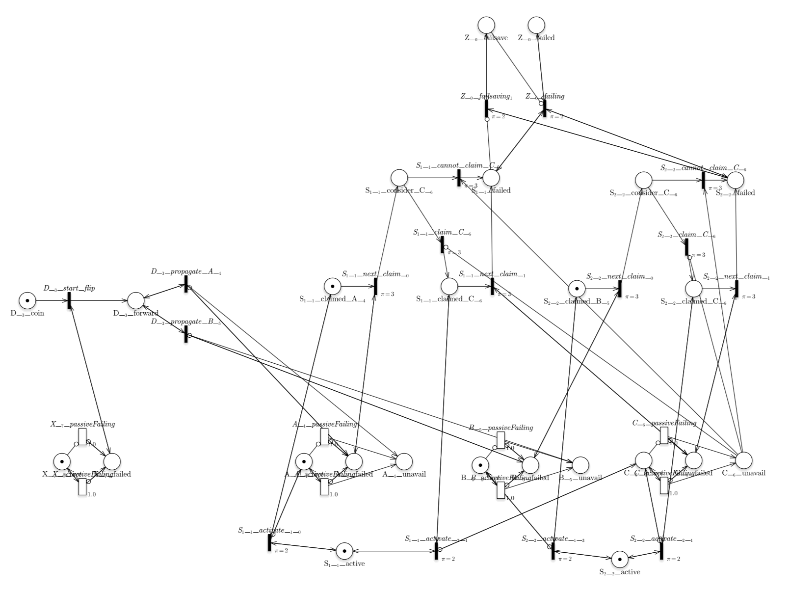
Figure 26: GSPN $\mathcal{T}_{\mathcal{F}_{3}}$ from GreatSPN Editor

References

- [1] Trivedi, K.S., Bobbio, A.: Reliability and Availability Engineering: Modeling, Analysis, and Applications. Cambridge University Press (2017)
- [2] Ruijters, E., Stoelinga, M.: Fault tree analysis: A survey of the state-of-the-art in modeling, analysis and tools. Computer Science Review 15-16 (2015) 29–62
- [3] Dugan, J.B., Bavuso, S.J., Boyd, M.: Fault trees and sequence dependencies. Proc. of RAMS, IEEE (1990) 286–293
- [4] Junges, S., Guck, D., Katoen, J.P., Stoelinga, M.: Uncovering dynamic fault trees. Proc. of DSN. (2016) 299–310
- [5] Marsan, M.A., Conte, G., Balbo, G.: A class of generalized stochastic Petri nets for the performance evaluation of multiprocessor systems. ACM TOCS 2(2) (1984) 93–122
- [6] Marsan, M.A., Balbo, G., Conte, G., Donatelli, S., Franceschinis, G.: Modelling with Generalized Stochastic Petri Nets. John Wiley & Sons (1995)
- [7] Raiteri, D.C.: The conversion of dynamic fault trees to stochastic Petri nets, as a case of graph transformation. ENTCS 127(2) (2005) 45–60
- [8] Bobbio, A., Raiteri, D.C.: Parametric fault trees with dynamic gates and repair boxes. Proc. of RAMS, IEEE (2004) 459–465
- [9] Bobbio, A., Franceschinis, G., Gaeta, R., Portinale, L.: Parametric fault tree for the dependability analysis of redundant systems and its high-level Petri net semantics. IEEE Trans. Softw. Eng. 29(3) (2003) 270–287
- [10] Kabir, S., Walker, M., Papadopoulos, Y.: Quantitative evaluation of Pandora Temporal Fault Trees via Petri Nets. IFAC-PapersOnLine 48(21) (2015) 458–463
- [11] Coppit, D., Sullivan, K.J., Dugan, J.B.: Formal semantics of models for computational engineering: a case study on dynamic fault trees. Proc. of ISSRE. (2000) 270–282
- [12] Boudali, H., Crouzen, P., Stoelinga, M.: A rigorous, compositional, and extensible framework for dynamic fault tree analysis. IEEE TDSC 7(2) (2010) 128–143
- [13] Volk, M., Junges, S., Katoen, J.P.: Fast dynamic fault tree analysis by model checking techniques. IEEE Trans. Industrial Informatics 14(1) (2018) 370–379
- [14] Eisentraut, C., Hermanns, H., Zhang, L.: On probabilistic automata in continuous time. Proc. of LICS, IEEE Computer Society (2010) 342–351
- [15] Hermanns, H.: Interactive Markov Chains: The Quest for Quantified Quality. Vol. 2428 of LNCS. Springer (2002)
- [16] Eisentraut, C., Hermanns, H., Katoen, J.P., Zhang, L.: A semantics for every GSPN. Petri Nets. Vol. 7927 of LNCS, Springer (2013) 90–109
- [17] Sullivan, K., Dugan, J.B., Coppit, D.: The Galileo fault tree analysis tool. Proc. of FTCS. (1999) 232–235
- [18] Arnold, F., Belinfante, A., van der Berg, F., Guck, D., Stoelinga, M.: DFTCalc: A tool for efficient fault tree analysis. Proc. of SAFECOMP. Vol. 8153 of LNCS. Springer (2013) 293–301
- [19] Dehnert, C., Junges, S., Katoen, J.P., Volk, M.: A Storm is coming: A modern probabilistic model checker. CAV (2). Vol. 10427 of LNCS, Springer (2017) 592–600
- [20] Trivedi, K.S., Sahner, R.A.: SHARPE at the age of twenty two. SIGMETRICS Performance Evaluation Review 36(4) (2009) 52–57
- [21] Ciardo, G., Miner, A.S., Wan, M.: Advanced features in SMART: the stochastic model checking analyzer for reliability and timing. SIGMETRICS Performance Evaluation Review 36(4) (2009) 58–63
- [22] Baarir, S., Beccuti, M., Cerotti, D., Pierro, M.D., Donatelli, S., Franceschinis, G.: The GreatSPN tool: recent enhancements. SIGMETRICS Performance Evaluation Review 36(4) (2009) 4–9
- [23] Amparore, E.G.: A new GreatSPN GUI for GSPN editing and CSLTA model checking. Proc. of QEST. Vol. 8657 of LNCS, Springer (2014) 170–173
- [24] Montani, S., Portinale, L., Bobbio, A., Raiteri, D.C.: Radyban: A tool for reliability analysis of dynamic fault trees through conversion into dynamic Bayesian networks. Rel. Eng. & Sys. Safety 93(7) (2008) 922–932
- [25] Boudali, H., Dugan, J.B.: A continuous-time Bayesian network reliability modeling, and analysis framework. IEEE Trans. Reliability 55(1) (2006) 86–97
- [26] Bouissou, M., Bon, J.L.: A new formalism that combines advantages of fault-trees and Markov models: Boolean logic driven Markov processes. Rel. Eng. & Sys. Safety 82(2) (2003) 149–163
- [27] Rauzy, A., Blériot-Fabre, C.: Towards a sound semantics for dynamic fault trees. Rel. Eng. & Sys. Safety 142 (2015) 184–191
- [28] Merle, G., Roussel, J.M., Lesage, J.J.: Quantitative analysis of dynamic fault trees based on the structure function. Quality and Rel. Eng. Int. 30(1) (2014) 143–156
- [29] Walker, M., Papadopoulos, Y.: Qualitative temporal analysis: Towards a full implementation of the Fault Tree Handbook. Control Eng Pract 17(10) (2009)
- [30] Chen, D., Mahmud, N., Walker, M., Feng, L., Lönn, H., Papadopoulos, Y.: Systems modeling with EAST-ADL for fault tree analysis through HiP-HOPS*. IFAC Proceedings Volumes 46(22) (2013) 91–96
- [31] Guck, D., Spel, J., Stoelinga, M.: DFTCalc: Reliability centered maintenance via fault tree analysis. ICFEM. Vol. 9407 of LNCS, Springer (2015) 304–311
- [32] Raiteri, D.C.: Integrating several formalisms in order to increase fault trees’ modeling power. Rel. Eng. & Sys. Safety 96(5) (2011) 534–544
- [33] Manian, R., Coppit, D.W., Sullivan, K.J., Dugan, J.B.: Bridging the gap between systems and dynamic fault tree models. Proc. of RAMS. (1999) 105–111
- [34] Engelfriet, J.: Branching processes of Petri nets. Acta Inf. 28(6) (1991) 575–591