How Problematic is the Near-Euclidean Spatial Geometry of the Large-Scale Universe?

Abstract

Modern observations based on general relativity indicate that the spatial geometry of the expanding, large-scale Universe is very nearly Euclidean. This basic empirical fact is at the core of the so-called “flatness problem”, which is widely perceived to be a major outstanding problem of modern cosmology and as such forms one of the prime motivations behind inflationary models. An inspection of the literature and some further critical reflection however quickly reveals that the typical formulation of this putative problem is fraught with questionable arguments and misconceptions and that it is moreover imperative to distinguish between different varieties of problem. It is shown that the observational fact that the large-scale Universe is so nearly flat is ultimately no more puzzling than similar “anthropic coincidences”, such as the specific (orders of magnitude of the) values of the gravitational and electromagnetic coupling constants. In particular, there is no fine-tuning problem in connection to flatness of the kind usually argued for. The arguments regarding flatness and particle horizons typically found in cosmological discourses in fact address a mere single issue underlying the standard FLRW cosmologies, namely the extreme improbability of these models with respect to any “reasonable measure” on the “space of all spacetimes”. This issue may be expressed in different ways and a phase space formulation, due to Penrose, is presented here. A horizon problem only arises when additional assumptions - which are usually kept implicit and at any rate seem rather speculative - are made.

1 Introduction

Though there never were a circle or triangle in nature, the truths demonstrated by Euclid would for ever retain their certainty and evidence.
David Hume [1]

It is a commonplace that Euclid’s theory of geometry, as layed down in the monumental, 13-volume Elements [2], reigned supreme for more than two millennia. The associated status of the theory, well reflected in the above quote by Hume, in fact pertained to both its apparent faithful characterization of the geometry of “physical space” and its axiomatic structure as a model for deductive reasoning. With the advent of non-Euclidean geometries in the nineteenth century, the geometrical nature of “physical space” became a question wide open and as famously emphasized by Riemann in his 1854 inaugural lecture [3], this question is ultimately to be decided by experiment. Nevertheless, Riemann’s programme only became in-principle feasible in the twentieth century, after Einstein - building heavily on some of Riemann’s geometrical ideas - revolutionized the classical notions of space, time and eventually gravitation through his two theories of relativity [4, *Einstein2]. Indeed, according to Einstein’s theory of general relativity, gravitation is viewed no longer as a force, but instead, as a manifestation of curved spacetime geometry. In order to address the geometrical nature of “physical spacetime”, it thus seems imperative to determine its curvature. As is well known, non-Euclidean geometries first appeared as alternatives to Euclidean plane geometry in which the parallel postulate was no longer assumed and it was found that they exist in two basic varieties, depending on the sign of a single curvature constant, $K$, namely the elliptic plane ($K>0$), characterized for instance by the convergent behaviour of initially parallel geodesics and the hyperbolic plane ($K<0$), characterized for instance by the divergent behaviour of initially parallel geodesics. Yet, the (Riemann) curvature of a four-dimensional spacetime geometry is in general specified in terms of twenty independent, non-constant parameters and according to general relativity only half of these parameters are directly (i.e., locally) expressable in terms of matter (or, more generally, non-gravitational “source”) degrees of freedom through Einstein’s field equation. In order to have a chance of arriving at an intelligible statement about spacetime’s actual geometry, it is necessary, obviously, to resort to an approximation, based on what is (arguably) the big picture. As will be recalled in section 2, when this is done, general relativity quite remarkably predicts a characterization of the global geometry of spacetime in terms of a single curvature constant, the meaning of which is completely analogous to that in the intuitive, two-dimensional case. Furthermore, and seemingly even more remarkable, the actually observed value of a particularly relevant cosmological observable, $\Omega$, is in fact close to the value corresponding to a flat, i.e., Euclidean, geometry [6]. This basic empirical fact is at the core of the so-called “flatness problem”, which is widely perceived to be a major problem of the standard Friedmann-Lemaître-Robertson-Walker (FLRW) cosmologies and as such forms one of the prime motivations behind the inflationary hypothesis that is part of the current $\Lambda\mbox{CDM}$ “cosmological concordance model”. An inspection of the literature and some further critical reflection however quickly reveals that the typical formulation of the flatness problem is fraught with questionable arguments and misconceptions and that it is moreover imperative to distinguish between different varieties of problem. As will be shown in detail in section 3, the observational fact that the large-scale Universe is so nearly flat is ultimately no more (or less) puzzling than similar “anthropic coincidences”, such as the specific (orders of magnitude of the) values of the gravitational and electromagnetic coupling constants. In particular, there is no fine-tuning problem. The usual arguments for the flatness and horizon problems found in inflationary discourses in fact address a mere single issue underlying the standard FLRW cosmological models. As will become clear in section 4, this particular issue becomes a genuine theoretical problem, one that is argued to require a dynamical mechanism such as inflation for its resolution, only under additional assumptions, which are usually kept implicit and are at any rate speculative. It will also become clear however that if these assumptions are not made, this does not imply that the effectiveness of the FLRW approximation poses no problem. In fact, a serious problem still remains, but it will require a type of solution that is radically different from dynamical mechanisms such as inflation, as a result of its very nature. For the benefit of the reader, section 2 consists of a brief, but mathematically concise review of FLRW models and their empirical basis. Geometrized units (i.e., $G_{\mbox{\scriptsize N}}:=1$, $c:=1$) are in effect throughout in what follows.

2 Isotropic Cosmologies

One of the most startling consequences of general relativity is that it almost inevitably leads to the notion of a dynamically evolving Universe. As is well known, it was Einstein himself who, when confronted with this situation in an attempt to model the Universe’s spatial geometry as a three-sphere, with matter distributed uniformly, sought to avoid this particular implication of his theory by introducing an additional, “cosmological constant” term into the field equation [7]. By carefully adjusting the value of the cosmological constant to a specific magnitude, the picture of a static, non-evolving Universe could be retained, but only so at the expense of conflicting with “naturalness” - as soon became clear through independent works of Friedmann [8] and Lemaître [9], most notably - and eventually of course also firm observational evidence in the form of Hubble’s law [10]. Although Einstein’s particular interpretation of a cosmological constant had thus become falsified by the late 1920s, whereas his arguments for a closed, elliptic spatial geometry were also generally regarded as unconvincing, what did survive in essentially unmodified form from the effort, was the picture of a Universe with matter distributed uniformly.
That is to say, underlying the dynamically evolving solutions obtained by Friedmann and Lemaître in the 1920s (or, for that matter, the current standard model of cosmology, which is fundamentally based upon these solutions), is the assumption that on sufficiently large spatial scales, the Universe is essentially isotropic, i.e., essentially “looks the same” in every direction at every point of “space”. Obviously, it is important to have a rough sense of the cosmological scales at which isotropy is thought to become effective. For instance, while typical galactic scales are absolutely enormous compared to any human scale (taking our Milky Way Galaxy - which measures $\sim$ 100,000 ly (roughly $10^{21}$ m) in diameter and is estimated to contain some $10^{11}$ stars, distributed in the form of a spiral-like, thin disk - as more or less representative, photons from stars on the opposite side of the Galaxy and incident upon Earth now, for instance, were emitted long before any human civilization existed), such scales are still tiny when compared to the overall scale of the observable Universe, which is another five orders of magnitude larger. While galaxies are also found to (super-)cluster on a wide range of scales and while at the same time there appear to be large regions effectively devoid of any galaxies (and apparently matter), observations indicate that on the largest cosmological scales, the Universe is isotropic to a very good degree of approximation. In particular, empirical support for isotropy comes from (i) direct astronomical observations of remote galaxies within optical and radio regions of the electromagnetic spectrum (including measurements of Hubble redshifts), (ii) indirect observations, such as the distribution pattern of cosmic rays incident upon Earth, and, most significantly, (iii) the extra-ordinary uniformity - i.e., up to a few parts in $10^{5}$ - of the Cosmic Microwave Background (CMB) [11, *WuLaRe, *Longair].
Although this observational evidence strictly speaking only indicates that the large-scale Universe is isotropic with respect to us (i.e., the Milky Way Galaxy), it is commonly considered bad philosophy since the time of Copernicus to take any such circumstance as evidence that we somehow find ourselves at a privileged (spatial) position. This very reasonable position, which thus in essence states that the large-scale Universe is spatially homogeneous, i.e., that at any “instant of time”, the observable features of other regions of the Universe (measured at sufficiently large scales) are effectively identical to those of our region, is also well supported by experimental data [14, *Sarkarcs]. Empirical evidence, together with common sense, thus strongly suggests that, to a very good degree of approximation, the large-scale observable Universe is spatially isotropic. As it turns out, such a uniformity condition is mathematically very restrictive and completely fixes the form of the spacetime metric, $g_{ab}$. For future reference, the most characteristic features of a spatially isotropic spacetime $(M,g_{ab})$ are briefly recalled here.

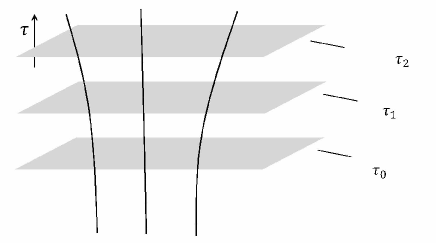
Figure 1: Foliation of a FLRW spacetime by hypersurfaces of homogeneity, $\Sigma_{\tau}$, representing different “instants of time”, $\tau$. These spatial geometries are orthogonally intersected by a congruence of timelike geodesics, which are the worldlines of isotropic observers (representing individual galaxies), and have constant curvature labeled by a discrete index $k\in\{-1,0,1\}$.

• $M$ is foliated by a family of spacelike hypersurfaces, $\Sigma_{\tau}$ , representing different “instants of time”, $\tau$, and there exists a preferred family of isotropic “observers” (i.e., galaxies) represented by a congruence of timelike geodesics with tangents, $u^{a}$, orthogonal to the surfaces of simultaneity (cf. Fig. 1 and footnote 5).

• Each spatial hypersurface is a space of constant curvature and the metric takes the Friedmann-Lemaître-Robertson-Walker (FLRW) form

  $$ds^{2}\;=\;-d\tau^{2}\>+\>a^{2}(\tau)\left(\frac{dr^{2}}{1-kr^{2}}\>+\>r^{2}d\omega^{2}\right)$$ (1)

  with $\tau$ denoting the proper time of galaxies, $a(\tau)$ representing an overall scale-factor of the homogeneous three-geometry, $\Sigma_{\tau}$ and $k$ a curvature constant which equals either $-1$, $0$, or $+1$, depending on whether the spatial geometry is respectively hyperbolic, Euclidean, or elliptic ($d\omega^{2}=d\theta^{2}+\sin^{2}\theta d\phi^{2}$, with $(r,\theta,\phi)$ denoting spherical coordinates as usual). In other words, the spatial geometry is essentially fixed once a value for $k$ is specified.

• The metric (1) is conformally flat, i.e., can be expressed in the form $\Upsilon^{2}\eta$, where $\eta$ denotes the standard Minkowski metric and $\Upsilon$ is a strictly positive (smooth) function. Hence, the Weyl tensor vanishes identically, $C^{a}_{\mspace{10.0mu}bcd}=0$, and there are no proper gravitational degrees of freedom in a FLRW spacetime.

• By virtue of the symmetry, the stress-energy tensor, $T_{ab}$, necessarily takes the perfect fluid form

  $$T_{ab}\;=\;\rho u_{a}u_{b}\>+\>P(g_{ab}+u_{a}u_{b})$$ (2)

  with $\rho$ and $P$ respectively denoting the (spatially constant) energy density and pressure of the fluid, as a result of which the ten, a priori independent, components of Einstein’s field equation

  $$G_{ab}\>+\>\Lambda g_{ab}\;:=\;R_{ab}\>-\>\frac{1}{2}Rg_{ab}\>+\>\Lambda g_{ab}\;=\;8\pi T_{ab}$$ (3)

  (with $R_{ab}$, $R$ and $\Lambda$ respectively denoting, as usual, the Ricci tensor, scalar curvature and cosmological constant) reduce to just two independent equations

  $$\frac{3\dot{a}^{2}}{a^{2}} = 8\pi\rho\>+\>\Lambda\>-\>\frac{3k}{a^{2}}$$ (4)

  $$\frac{3\ddot{a}}{a} = -4\pi(\rho\>+\>3P)\>+\>\Lambda$$ (5)

  where the dot denotes differentiation with respect to proper time. Eq. (4) is usually referred to as the Friedmann equation. Together with Eq. (5), it implies

  $$\dot{\rho}\>+\>3\left(\rho\>+\>P\right)\frac{\dot{a}}{a}\;=\;0$$ (6)

  (alternatively, Eq. (6) is the component of the equation of motion of the fluid, $\nabla^{a}T_{ab}=0$, parallel to the congruence).

In order to determine the dynamical behaviour of the scale factor, $a$, as a function of pressure, $P$, and energy density, $\rho$, of the cosmic fluid, it is necessary to posit an equation of state, i.e., a functional relationship between $P$ and $\rho$, that allows elimination of $P$ from Eq. (6) and subsequent expression of $\rho$ as a function of $a$. Usually such an equation of state is simply assumed to be linear, i.e.,

$$P\;=\;w\rho$$ (7)

for a constant proportionality factor, $w$, which in the following is taken to be non-negative. Integration of Eq. (6) then gives

$$\rho\;=\;Ca^{-3(1+w)}$$ (8)

with $C\geq 0$ an arbitrary constant and the Friedmann equation becomes

$$\dot{a}^{2}\;=\;\frac{8\pi}{3}Ca^{-(1+3w)}\>+\>\frac{\Lambda a^{2}}{3}\>-\>k$$ (9)

General solutions to Eq. (9) for various cases of physical interest can be written down explicitly (some in terms of elementary functions), but it suffices here to restrict attention to the two most important generic features of solutions in relation to the present discussion:

• All physically relevant FLRW models - i.e., models that are (at least at some stage) effectively “non-empty” ($C>0$) and have sufficiently large, positive cosmological constant, $\Lambda$ - are non-static and start with a “Big-Bang”, i.e., a singularity, $a=0$, at $\tau=0$

• For small $\tau$, the dynamical trajectories of all FLRW models with an initial singularity tend to the corresponding trajectories of $k=0$, $\Lambda=0$ models (as can in fact be read off directly from the Friedmann equation in the form (9)). In particular, regardless of spatial geometry and the value of the cosmological constant, at early times all past-singular solutions for dust tend to $\tau^{2/3}$ (Einstein-de Sitter solution), whereas all past-singular solutions for radiation tend to $\tau^{1/2}$

As will be seen in the next section, both these features play a critical role in what is widely perceived to be a serious shortcoming of FLRW models as applied to the actual Universe.

3 Problems of Flatness - Inflated and Otherwise

Fundamental to most discussions of the putative flatness problem(s) is the Friedmann equation (4) rewritten in the following form

$$\Omega_{\mathrm{m}}\>+\>\Omega_{\Lambda}\;=\;1\>+\>\frac{k}{\dot{a}^{2}}\;=\;1\>+\>\frac{k}{H^{2}a^{2}}$$ (10)

where the dimensionless parameters $\Omega_{\mathrm{m}}:=8\pi\rho/3H^{2}$ and $\Omega_{\Lambda}:=\Lambda/3H^{2}$ respectively measure the density of matter, $\rho$, and the (suitably normalized) cosmological constant, $\Lambda/8\pi$, in terms of the “critical density”, $\rho_{\mathrm{c}}:=3H^{2}/8\pi$ (see below), and where $H:=\dot{a}/a$ denotes Hubble’s “constant”. Historically, the line of argument that was taken to establish a “flatness problem” first emerged in the late 1970s, when (in absence of empirical evidence to the contrary) the cosmological constant was typically taken to vanish and for simplicity this context will be dealt with first in subsection 3.1 below (as will also become clear however, inclusion of nonzero $\Lambda$ does not change anything as far as this particular line of argument is concerned). On setting $\Lambda=0$, it is immediately clear from Eq. (10) that $\rho_{\mathrm{c}}$ is indeed a critical density required for an “open universe”. That is, a FLRW model is necessarily “closed” (spatial geometry of finite extension, corresponding to $k=+1$) if $\rho>\rho_{\mathrm{c}}$, whereas it is usually called “open” (spatial geometry of infinite extension, corresponding to $k=-1$ or $k=0$) if $\rho\leq\rho_{\mathrm{c}}$. Moreover, unlike the possible models with nonzero curvature, the $\Omega$-parameter for the critical case, corresponding to a flat, Euclidean spatial geometry, is identically constant, i.e., $\Omega_{\mathrm{m}}=1$ at all times. Now, the actual observed value of $\Omega_{\mathrm{m}}$ at present is known to be close to unity [6] - i.e., close to the constant value corresponding to a Euclidean geometry - and the flatness problem of FLRW cosmologies, broadly construed, is perceived to be the apparent “improbability” of this basic empirical truth.
In fact, a critical inspection of the relevant literature indicates that there are at least three different formulations of the flatness problem and although these formulations are related to each other (and not infrequently also conflated), they are ultimately distinct. A basic classification of (alleged) flatness problems can be made depending on whether dynamical arguments are involved or not. Those that do are found to exist in two standard versions (which, somewhat ironically, are logically complementary to each other), namely (i) a perceived problem of exceeding unlikeliness that $|\Omega_{\mathrm{m}}-1|$, if in fact nonzero, was very nearly “almost” zero - i.e., to within a very large number of decimal places - at very early times, given that $\Omega_{\mathrm{m}}\simeq 1$ at present (fine-tuning argument) and (ii) a perceived problem of exceeding unlikeliness that, in the non-critical case, $\Omega_{\mathrm{m}}\simeq 1$ at present, given that $|\Omega_{\mathrm{m}}-1|$ was “extremely close” to zero at very early times (instability argument). Non-dynamical versions of the flatness problem on the other hand are essentially variations on the theme of why fundamental physical parameters, such as Newton’s constant, $G_{\mbox{\scriptsize N}}$, or the fine-structure constant, $\alpha$, take the particular values they do.

3.1 The Fine-Tuning Argument

According to the prevailing wisdom, in order that the value of $\Omega_{\mathrm{m}}$ be anywhere near $1$ today, it had to be extremely delicately “adjusted” in the very early Universe. There is then an arguable necessity to identify the relevant physical laws responsible for such an alleged “fine-tuning” and it is often argued in this regard that “inflationary physics” has the potential to provide a resolution (see section 4). The essential steps of the argument are to derive from the Friedmann equation (10) the following identity

$$\left(\Omega_{\mathrm{m}}(\tau^{\prime})\>-\>1\right)\;=\;\left(\Omega_{\mathrm{m}}(\tau)\>-\>1\right)\frac{\dot{a}^{2}_{\tau}}{\dot{a}^{2}_{\tau^{\prime}}}$$ (11)

(where $\tau$ and $\tau^{\prime}$ explicitly display the proper time dependence of quantities but are further arbitrary) and to note that Eq. (5) (in the present context with $\Lambda=0$, $C>0$ and $w\geq 0$) implies

$$\ddot{a}\;<\;0$$ (12)

at all times. Since $\dot{a}$ blows up at the origin, this means that for fixed $\tau$ and sufficiently small $\tau^{\prime}$, one has $\dot{a}^{2}_{\tau}/\dot{a}^{2}_{\tau^{\prime}}\ll 1$. Thus, if $\tau$ denotes the present epoch, for which $\Omega_{\mathrm{m}}$ differs from $1$ by, say, a number of order unity, it directly follows from Eq. (11) that the deviation of $\Omega_{\mathrm{m}}$ from $1$ in the very early Universe had to be “extremely small”

$$|\Omega_{\mathrm{m}}(\tau^{\prime})\>-\>1|\;\ll\;1$$ (13)

so that (according to this argument) $\Omega_{\mathrm{m}}(\tau^{\prime})$ had to be seriously “fine-tuned” in some way.

Some Numerology

It is instructive to consider a few standard examples with explicit, numerical estimates of the amount of putative fine-tuning of $\Omega_{\mathrm{m}}$. First, since $\Omega_{\mathrm{m}}$ is presently close to $1$, it is (tacitly) assumed that the $k=0$ solutions provide a good approximation. Taking this assumption to be valid (if only for the sake of argument) and using the explicit solutions for dust (i.e., $a\sim\tau^{2/3}$) and radiation (i.e., $a\sim\tau^{1/2}$) in this case, Eq. (11) rewrites to

$$\left(\Omega^{\prime}_{m}\>-\>1\right)\;=\;\left(\Omega_{\mathrm{m}}\>-\>1\right)\left(\frac{\tau^{\prime}}{\tau}\right)^{2/3}\qquad\mbox{and}\qquad\left(\Omega^{\prime}_{m}\>-\>1\right)\;=\;\left(\Omega_{\mathrm{m}}\>-\>1\right)\frac{\tau^{\prime}}{\tau}$$ (14)

respectively. Taking $\tau\simeq 13.8\,\mbox{Gy}\simeq 10^{17}\,\mbox{s}$, $\tau_{\mbox{\scriptsize eq}}\simeq 40\,\mbox{ky}\simeq 10^{12}\,\mbox{s}$ and $\Omega_{\mathrm{m}}\simeq 0.3$ as representative values for respectively the current age of the Universe, the age of the Universe when matter started to become dominant over radiation and the (normalized) density of matter corresponding to the current epoch, this then leads to a “fine-tuning” of $\Omega_{\mathrm{m}}$ to $1$ to an accuracy of

$$\mbox{one part in}\;10^{16}$$ (15)

if $\tau^{\prime}$ is taken to be of the order of a second. Similarly, $\Omega_{\mathrm{m}}$ is “fine-tuned” to $1$ to an accuracy of

$$\mbox{one part in}\;10^{59}$$ (16)

if $\tau^{\prime}$ is taken to be of the order of the Planck time $\simeq 10^{-43}\,\mbox{s}$.

As just presented, the fine-tuning argument is the most commonly encountered line of reasoning - often also the only one considered - purported to establish a flatness problem. Going back to an early argument (made somewhat less explicitly) by Dicke and Peebles [26], it was subsequently emphasized by Guth and others as a key motivation for introducing inflationary models [27, *Linde3, *Albstein] and has been viewed as signalling a major drawback of the standard FLRW models by probably most cosmologists ever since. It is however a seriously problematic argument - as was in fact already pointed out in different ways by various authors on previous occasions [36], [37], [38], [39], [40, *Helbig2], [42]. The essential point is that the near-magical “fine-tuning” exhibited by Eqs. (15), (16), is nothing but a consequence of the Friedmann dynamics (10) (or, equivalently, Eq. (4)). Indeed, as stressed in the previous section (cf. the discussion below Eq. (9)), all cosmologically relevant FLRW models necessarily become indistinguishable from flat FLRW models in the limit of small $\tau$, in the sense that $\Omega_{\mathrm{m}}=1$ exactly at $\tau=0$. This for instance follows directly from Eq. (10), since $\dot{a}$ diverges for $\tau\rightarrow 0$; alternatively, it follows from expressing $\Omega_{\mathrm{m}}$ in terms of the scale factor, $a$, using Eqs. (8), (9), i.e.,

$$\Omega_{\mathrm{m}}\;=\;\frac{8\pi C}{8\pi C-3ka^{1+3w}}$$ (17)

In other words, the “fine-tuning” is a feature that is inherent to all these models. In particular, it also occurs in those instances where $\Omega_{\mathrm{m}}$ is not close to $1$ after $\simeq 10^{17}\,\mbox{s}$ (for instance, it is easily checked that solutions for which $\Omega_{\mathrm{m}}$ has become significantly smaller than $1$ after this time are “fine-tuned” to the same fantastic precision - i.e., to $59$ decimal places in the above example - at the Planck scale in this sense just as well; clearly $|\Omega_{\mathrm{m}}-1|_{\mbox{\scriptsize present}}$ is of order $1$ for all values of $\Omega_{\mathrm{m}}$ of order $10^{-N}$, $N\geq 0$). There is thus no problem of fantastic improbability, since initial conditions could not have been otherwise within the present context.
It is useful to slightly elaborate upon this point, since it is sometimes contended that $\Omega_{\mathrm{m}}$ could have had any initial value (see some of the earlier quoted references for explicit statements to this effect). As the foregoing shows, within the strict context of isotropic cosmologies, this contention is simply false. Although actually underlying the claim is a different context (which is usually not very clearly spelled out), the conclusion that there is no fine-tuning problem is unaffected. First, as various authors have pointed out, the assumption that the set of possible initial values for $\Omega_{\mathrm{m}}$ is significantly larger and governed by a sufficiently uniform probability distribution can well be criticized on general methodological grounds [36], [40, *Helbig2], [43]. In fact, such a view is also supported by a sober analysis of a more explicit picture of initial conditions.
That is, even though a consistent, physical theory of “quantum gravity” is yet to be formulated, it is often argued that the classical picture of spacetime as described by general relativity should reasonably be expected to break down near the Planck scale. If it is assumed that the FLRW context provides an acceptable description of spacetime geometry all the way down to the Planck time $\sim 10^{-43}\,\mbox{s}$ - which is what most of those who argue for an actual independent flatness problem seem perfectly content with (given their numerological arguments at least) - and if the set of possible “initial” values for $\Omega_{\mathrm{m}}$ at this time is allowed to be very general, say $\mathbb{R}^{+}$, it is certainly true that $|\Omega_{\mathrm{m}}-1|\simeq 10^{-59}$ (or some similar small number) as an initial condition appears extremely unnatural at first glance. What is often not realized however is that there is a sharp “trading off” between genericity in an initial value of $\Omega_{\mathrm{m}}$ at the Planck scale and genericity in the parameter $C$ residing in $\Omega_{\mathrm{m}}$ (and similarly for other FLRW models with different matter contents). The reason is simply that FLRW solutions, in order to prevent their duplication, display a one-to-one correspondence between possible “initial” values of $\Omega_{\mathrm{m}}$ at the Planck scale $\sim 10^{-43}\,\mbox{s}$ (i.e., $0<\Omega_{\mathrm{m}}<1$ for $k=-1$ and $1<\Omega_{\mathrm{m}}<\infty$ for $k=+1$) and possible values of $C$. In particular, the more generic an initial value for $\Omega_{\mathrm{m}}$, the more fine-tuning in $C$ would be required to achieve this. As can readily be verified from Eq. (17), for generic values of $C$ (as picked at random, say, by an unskilled, blindfolded Creator), $\Omega_{\mathrm{m}}$ will still be fine-tuned to the fantastic number of decimal places (16) at the Planck scale.
The fact that spatial geometry could be highly anisotropic at pre-Planckian timescales - as seems to be envisaged in many currently popular approaches - is irrelevant here. Although it is prima facie unclear how to extend the notion of a (single) “critical density” - and hence the definition of $\Omega_{\mathrm{m}}$ - in a meaningful way to general anisotropic models (for homogeneous models it is still possible to define an average Hubble constant [44]), if a more general set of initial values for $\Omega_{\mathrm{m}}$ is envisaged to (somehow) carry physical meaning, the enormous “fine-tuning” of $\Omega_{\mathrm{m}}$ is a mere artefact of the particular construction at hand and would in itself thus establish nothing. This is because any (cosmologically relevant) model for which $\Omega_{\mathrm{m}}$ is not so “fine-tuned” cannot be a FLRW model and hence, the tacit underlying issue here is that of natural probability assignment to FLRW models in some “sufficiently large space of theoretically consistent cosmological models” (and obviously, the exact same argument can be made for models that are “almost isotropic”; these would also have to be sufficiently “fine-tuned”).
As will be discussed further in section 4, although there are indeed good grounds to argue that FLRW models are in some sense “improbable”, these grounds, being fundamentally based on the second law of thermodynamics, are rather different from the type of probabilistic reasoning that is usually encountered in this context. In fact, as will become clear from this particular perspective on things, it is highly unlikely that the improbability of FLRW initial conditions in the sense intended, can be succesfully resolved merely in terms of dynamical arguments (as invariably called upon in response to the more usual kind of improbability claims). But whichever particular perspective is adopted, all probabilistic arguments relevant here merely address the overall context of isotropy. Once within that context, a “fine-tuning” of $\Omega_{\mathrm{m}}$ and the existence of particle horizons (see section 4) are inevitable features of all cosmologically relevant models. This thus means that there is no independent problem of flatness of the fine-tuning variety.
As is easily verified, this conclusion is completely general, despite the fact that the cosmological constant, $\Lambda$, was ignored in the foregoing. Using again Eq. (9), the parameter $\Omega_{\Lambda}$ of Eq. (10) can be expressed directly in terms of the scale factor

$$\Omega_{\Lambda}\;:=\;\frac{\Lambda}{3H^{2}}\;=\;\frac{\Lambda a^{3(1+w)}}{8\pi C+\Lambda a^{3(1+w)}-3ka^{1+3w}}$$ (18)

from which it follows that $\Omega_{\Lambda}\rightarrow 0$ for $a\rightarrow 0$ (for $\Omega_{\mathrm{m}}$, an additional term $\Lambda a^{3(1+w)}$ now also has to be included in the denominator of expression (17), but this term obviously does not affect the limiting behaviour of $\Omega_{\mathrm{m}}$ at $a=0$). Thus, if near-flatness is understood in the (physically more appropriate) sense of “closeness to $1$” of the total $\Omega$-parameter, i.e., $\Omega:=\Omega_{\mathrm{m}}+\Omega_{\Lambda}$, rather than in terms of the approximate equality of the density of matter to the critical density, the same calculation as before now gives that $\Omega$ differed from $1$ by a number of order $10^{-62}$ at the Planck scale, if its present deviation from $1$ is $\lesssim 10^{-3}$ [6]. Inclusion of an actual, physically relevant cosmological constant term only increases slightly the level of putative fine-tuning; it does not in any way affect the previous conclusion that there is no independent fine-tuning problem to begin with.

3.2 The Instability Argument

A more sophisticated argument purporting to establish the problematic nature of the near-flatness of the Universe’s large-scale spatial geometry essentially consists of the claim that given that (to a fantastic number of decimal places) the initial density of matter, $\rho$, equaled the critical density, $\rho_{\mathrm{c}}$, or, alternatively, that the initial value of (total) $\Omega$ was equal to $1$, it is not to be “expected” that (within an order of magnitude, say) $\rho$ would still be “close” to $\rho_{\mathrm{c}}$, or, alternatively, that $\Omega\simeq 1$, after some fourteen or so billion years of cosmic evolution (see e.g. Ref. [45, *Smeenk, *SmEl] for an argument along these lines). Given that $\rho$ necessarily evolves away from $\rho_{\mathrm{c}}$ with time (for nonzero $k$), i.e., $\Omega=1$ is an unstable fixed point of the FLRW dynamics, this seems a prima facie plausible argument (although, as already mentioned, different types of arguments pertaining to flatness are typically conflated in the literature - something which is in particular true for the instability and fine-tuning varieties). Upon closer inspection however, this argument is also found to evaporate into thin air. First, if the present closeness of $\Omega$ to $1$ is accepted as basic empirical input and the approximations used in section 3.1 are again taken to be valid, it is clear that there can be no probability problem in a restricted sense, since the (deterministic) FLRW dynamics works both ways. In order for this type of argument to be potentially successful, it is necessary to consider a significantly more general framework, in which models where $\Omega$ remains “close to $1$” for “sufficiently long” either do not exist or can somehow be securely classified as being highly non-generic. This however does not appear to be possible. (Note that even if the instability argument were sound, a dynamical mechanism, such as inflation, designed to drive spatial geometry to near-flatness at extremely early times, would by its very nature be useless to address this argument.)
For instance, for a cycloidal universe (i.e., a dust-filled model with positive curvature and zero cosmological constant; $w=\Lambda=0$, $k=+1$), it is easily checked that $\Omega_{\mathrm{m}}<10$ for a full $60\%$ of its total lifespan, even though $\Omega_{\mathrm{m}}$ is in fact unbounded. Fictitious theorists in such a hypothetical universe would thus presumably conclude that there was nothing improbable to explain if observations were in fact to indicate that $\Omega_{\mathrm{m}}<10$, since probabilities for observing different ranges of $\Omega_{\mathrm{m}}$-values are evidently distributed in a highly non-uniform fashion.
In view of the actual constraints placed on the present value of $\Omega_{\mathrm{m}}$ by observations (which exclude the possibility that $1<\Omega_{\mathrm{m}}<10$) and, more generally, in view of the oscillatory nature of the cycloidal universe, the example just presented is of course rather unrealistic on physical grounds. Yet, it serves well to illustrate the point that something which may seem a priori obvious (i.e., the idea that the cycloidal universe would be “far more probable” to reside in the infinite region $10<\Omega_{\mathrm{m}}<\infty$, than in the finite region $1<\Omega_{\mathrm{m}}<10$, both regions being traversed twice), need not in fact be true. Furthermore, a similar line of argument can be used to establish that there is no manifest probability problem in the non-oscillatory case either (see Ref. [20] for a discussion of both the cycloidal and non-cycloidal cases), something which is intuitively obvious from the expression for the total $\Omega$-parameter

$$\Omega\;:=\;\Omega_{\mathrm{m}}\>+\>\Omega_{\Lambda}\;=\;\frac{8\pi C+\Lambda a^{3(1+w)}}{8\pi C+\Lambda a^{3(1+w)}-3ka^{1+3w}}$$ (19)

Indeed, it is clear from this expression that for cosmologically relevant models, $\Omega=1$ is both a repulsor (i.e., at $a=0$) and an attractor (i.e., for $a\rightarrow\infty)$ of the dynamics and it is therefore not obviously “strange” or improbable if the value of $\Omega$ should happen to be observed near $1$ at some intermediate time, e.g. at $13.8\,\mbox{Gy}$. In fact, a rigorous analysis of possible dynamical trajectories in the $\Omega_{\mathrm{m}}\Omega_{\Lambda}$-plane, taking into account actual observational constraints on these parameters from precision measurements of the CMB and of type IA supernovae, fully confirms this intuitive argument. To this end, it is useful to introduce a new, dimensionless time parameter according to $\eta:=\ln(a/a_{0})$, $a_{0}$ denoting some fixed reference value for the scale factor, here taken to correspond to the present epoch. This thus means that ${}^{\prime}:=d/d\eta=H^{-1}d/d\tau$ and on taking the case of dust ($w=0$) to be representative, Eqs. (4), (5) imply that $(\Omega_{\mathrm{m}},\Omega_{\Lambda})$ satisfy the following autonomous system of first-order differential equations

$$\Omega_{\mathrm{m}}^{\prime} = (\Omega_{\mathrm{m}}-2\Omega_{\Lambda}-1)\Omega_{\mathrm{m}}$$ (20)

$$\Omega_{\Lambda}^{\prime} = (\Omega_{\mathrm{m}}-2\Omega_{\Lambda}+2)\Omega_{\Lambda}$$ (21)

Conversely, Eqs. (20), (21) imply Eqs. (4), (5) for $P=0$ and hence the system (20), (21) constitutes an equivalent specification of the FLRW dynamics in the case of dust. Nontrivial critical points of (20), (21) are a repulsor (or negative attractor) at $(\Omega_{\mathrm{m}},\Omega_{\Lambda})=(1,0)$, corresponding to the Big Bang and a (positive) attractor at $(\Omega_{\mathrm{m}},\Omega_{\Lambda})=(0,1)$, corresponding to an asymptotic de Sitter phase. It is straightforward to check that the function $\alpha$, defined by

$$\alpha\;=\;\mp\frac{27\Omega^{2}_{\mathrm{m}}\Omega_{\Lambda}}{4\Omega_{k}^{3}}\qquad\quad\mbox{for}\;\;k=\pm 1,\quad\Omega_{\mathrm{m}}\geq 0,\quad\Omega_{\Lambda}\geq 0,\quad\Omega_{k}:=-k/\dot{a}^{2}$$ (22)

is a first integral of the system (20), (21) (note that for any FLRW solution, $\Omega_{k}=1-\Omega_{\mathrm{m}}-\Omega_{\Lambda}$). That is, the derivative of $\alpha$ along any orbit of (20), (21) vanishes

$$\alpha^{\prime}\;=\;\frac{\partial\alpha}{\partial\Omega_{\mathrm{m}}}\Omega_{\mathrm{m}}^{\prime}\>+\>\frac{\partial\alpha}{\partial\Omega_{\Lambda}}\Omega_{\Lambda}^{\prime}\;=\;0$$ (23)

and $\alpha$ is thus a constant of the motion.

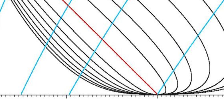
Figure 2: Partial Phase Portrait of $w=0$ FLRW Dynamical Trajectories. The straight line segment represents a flat FLRW model and separates the hyperbolic ($k=-1$) and elliptic ($k=+1$) models within the phase plane (which respectively lie to the left and to the right of the $k=0$ model as it is traversed into the future). Depicted in black are fourteen level sets of $\alpha$ that approach the delimiter from below, respectively above, for the subsequent values $\alpha=6,8,12,20,40,100,500$. The delimiter itself corresponds to $\alpha=\infty$. The dynamical trajectories are traversed by level sets of $tH$, here shown (in blue), from right to left, for the values $tH=2/3,3/4,0.826,1,3/2$. The particular values for $\alpha$ and $tH$ are partially informed by the results from WMAP and HST (cf. Ref. [39]). Level sets of $\alpha$ corresponding to lower bound values in accordance with the more recent Planck data have not been included, since these are near-indistinguishable from the $\alpha=\infty$ delimiter.

Fig. 2 depicts a family of level sets $\alpha=\mbox{constant}$ in a partial phase plane, intersected by a number of level sets of $tH$, where $t$ denotes the age of the Universe

$$t\;=\;\frac{1}{H}\,\int^{1}_{0}\frac{dx}{\sqrt{\Omega_{\mathrm{m}}x^{-1}+\Omega_{\Lambda}x^{2}+1-\Omega_{\mathrm{m}}-\Omega_{\Lambda}}}$$ (26)

The straight line segment $\Omega_{\Lambda}=1-\Omega_{\mathrm{m}}$, representing a flat FLRW model, is asymptotically approached from below, resp. above, by the hyperbolic (i.e., $k=-1$), resp. elliptic (i.e., $k=+1$) FLRW models in the large-$\alpha$ limit. The significance of these remarks is that CMB precision measurements strongly suggest that the $w=0$ FLRW model that best describes our Universe in its current phase is one for which $\alpha$ is very large. To the extent that such a model can be taken as a good approximation for the Universe during its entire evolution, it is then clear that there is no probability/instability problem, since such a model has $\Omega$ (as defined by Eq. (19)) close to unity throughout its entire history. As will be seen shortly however, this conclusion is in fact of much more general validity and in particular also pertains to FLRW models that went through a transition from a radiation-dominated epoch at early times, to a matter-dominated epoch (in the form of dust) at late times - as is estimated to have occurred in our actual Universe, about $380,\!000$ years after the Big Bang.
The above argument, linking the large value of the FLRW constant of the motion (22) implied by cosmological observations, to the flatness issue, first appears to have been made by Lake over a decade ago [39]. At that time, the results from the Wilkinson Microwave Anisotropy Probe (WMAP) and the Hubble Space Telescope (HST) on respectively CMB anisotropies and type IA supernovae, constrained curvature to vanish at $10^{-1}$ order ($95\%\,\mbox{CL}$), corresponding to a value of $\alpha$ of order $\gtrsim 500$ (i.e., the largest level set value in Fig. 2) [48, *Riessetal]. More recently, precision data from the Planck collaboration, in particular regarding CMB temperature (TT) and polarization (EE) power spectra and CMB lensing, in combination with BAO constraints, have been taken to imply that $|\Omega_{k}|\lesssim 5\times 10^{-3}$ [6]. Obviously, this corresponds to a huge increase in the lower bound on $\alpha$, i.e.,

$$\alpha\;\gtrsim\;3,\!000,\!000$$ (27)

(this more accurate constraint has not been included in Fig. 2, essentially because the corresponding level sets would blur into the delimiter representing the flat model). It should be stressed that the foregoing argument is of general validity, despite the fact that it was set up for the special case of dust, i.e., $w=0$ (the reason for having explicitly considered this special case is clearly that the argument is then relatively simple and moreover readily visualized). More precisely, given any FLRW model that incorporates an arbitrary number of non-interacting “particle” species with densities $\rho_{i}$, satisfying an equation of state of the form $p_{i}=w_{i}\rho_{i}$, with $w_{i}$ constant and distinct for each species, a complete set of FLRW constants of the motion can be explicitly constructed [51]. The crucial point is now that, as long as no species are removed, higher-order FLRW models (i.e., with larger numbers of species) inherit all constants of the motion from corresponding lower-order FLRW models. Thus, in the physically more accurate case of a FLRW model including both dust and radiation ($w_{\gamma}=1/3$), $\alpha$, as defined by Eq. (22), is still a constant of the motion and the fact that, as the Planck data strongly suggest, this constant of the motion is large, i.e., satisfies (27), means that its level surface in the full phase space always remains very close to the $\Omega_{\mathrm{m}}+\Omega_{\Lambda}+\Omega_{\gamma}=1$ plane representing the flat FLRW model in this case.
A final point worth mentioning is the following. As the preceding discussion shows, the Universe we inhabit happens to be best described by a large-$|\alpha|$ FLRW model. One could still ask how special such a model is however. Or, put differently, how generic are FLRW models with $\Omega_{\mathrm{m}}+\Omega_{\Lambda}\simeq 1$ throughout their history? As was recently shown by Helbig [40, *Helbig2] (recall also the discussion immediately preceding Eq. (19) above), the answer to this latter question is that such models are indeed very generic. In particular, temporally open models that are not always nearly flat are necessarily elliptic and satisfy $\alpha\approx 1$. In other words, the fine-tuning is reversed: models that are not almost flat throughout their history are necessarily fine-tuned.

3.3 $\Omega\simeq 1$ as an Anthropic Coincidence

A final version of the flatness problem sometimes encountered (although, again, conflations with the two previously discussed arguments are not uncommon) is based on the observation that spatial flatness appears to be an “anthropic coincidence”. That is, a universe in which $\Omega$ is smaller or larger than unity by significantly more than an order of magnitude would (presumably) be completely unlike the Universe as actually observed; in particular, such a hypothetical universe would (presumably) not be consistent with the existence of life in the form we know it (see e.g. Ref. [52] and references therein for an argument along these lines). Similar observations have been made regarding other basic parameters used in physical theory, i.e., Newton’s constant, $G_{\mbox{\scriptsize N}}=6.7\times 10^{-11}\mbox{N}\mbox{m}^{2}\mbox{kg}^{-2}$, the electron charge, $e=1.6\times 10^{-19}\,\mbox{C}$ (or the fine-structure constant, $\alpha:=e^{2}/4\pi\hbar c\simeq 1/137$), Fermi’s constant, $G_{\mbox{\scriptsize F}}=1.4\times 10^{-62}\mbox{J}\mbox{m}^{3}$ and so on. The issue as to whether such observations are to be interpreted as constituting an actual problem (and if so, what the extent of this problem is) is at the basis of one of the most vigorously debated topics in theoretical physics over the past decades.
One could say that the particular (orders of magnitude of) parameter values observed are simply a precondition for our existence - so that it is not at all surprising that we actually happen to observe these values - and just leave it at that. This so-called (weak) “anthropic reasoning” is perfectly self-consistent, but many physicists who feel that a deeper explanation of the observed coincidences somehow must exist, have in recent decades, rather controversially, invoked strong anthropic arguments to defend a “multiverse” concept of physical reality. This is obviously not the place to go into this contentious subject matter in detail , but in relation to the present discussion two key points should be stressed.
First, it might be thought that treating flatness as an “anthropic coincidence” in essentially non-dynamical terms is illegitimate, since $\Omega$, of course, actually is a dynamical parameter. The point here however is not to deny that $\Omega$ is a dynamical parameter, but rather that the fact that it is, is irrelevant for anthropic considerations based on the fact that $\Omega\simeq 1$. After all, the mathematical question of whether a particular value of $\Omega$ at some particular time is in some definite sense probable or not is objectively different from the metaphysical question of whether one should be surprised to observe a particular value for $\Omega$ (or any other relevant parameter), if that value happens to be a precondition for one’s existence. Moreover, although it is sometimes contended (conflation of different flatness arguments) that had $\Omega$ in fact been “fine-tuned” at the Planck scale to for instance five decimal places more or less than its presently calculated value, it would no longer be $\simeq 1$ after $\simeq 10^{17}\mbox{s}$, such a representation of things is obviously incorrect in view of the results discussed in subsection 3.2. Indeed, as those results made clear, FLRW models for which $\Omega\simeq 1$ throughout their entire history are in a well defined sense generic and so notwithstanding the fact that the “anthropic window” $0.1\lesssim\Omega\lesssim 10$ may appear to be small, values outside this window are in an appropiate sense much less probable (cf. also the earlier example of the $60\%$ window $1<\Omega_{\mathrm{m}}<10$ in the cycloidal universe).
The second key point about anthropic arguments in connection to the present discussion bears on the wider issue of “context of discovery” versus “context of justification” of these arguments, as well as that of the two other pillars of the modern trinity consisting of string/M-theory, (eternal) inflation and “multiverse”. As has become evident from the discussion in this section, in the case of inflation at least part of the former context is theoretically unsound and this evidently raises questions about the remaining part and about the context of justification. These issues, together with various pieces of evidence against discovery-context arguments for string/M-theory and the “multiverse”, are briefly discussed in the next section.

4 The Issue of Initial Conditions

According to Eq. (5), an expanding FLRW model with $\rho+3P\geq 0$ and $\Lambda\leq 0$ must start off in a singular state, $a=0$. Indeed, any FLRW model that is expanding at a constant rate, becomes past-singular at a finite prior time $H^{-1}$ and so any FLRW model that is expanding at a decelerating rate has to become past-singular in a time less than $H^{-1}$. Obviously, this argument is blocked if either $\rho+3P<0$ or $\Lambda>0$. However, all viable, classical cosmological models known to date satisfy $\rho+3P>0$ (which is essentially just another way of saying that these models satisfy the “strong energy condition” that the stress-energy tensor contracted with any unit timelike vector field is bounded from below by minus one half its trace), while even though $\Lambda>0$ for the observable Universe in its present state, this does not in fact prohibit reversing the trend of contraction in the past time direction. In other words therefore, all cosmologically relevant classical FLRW models start with a “Big Bang” a finite amount of time ago. As is well known, according to one of the celebrated Hawking-Penrose singularity theorems [55], this conclusion extends to all general relativistic models that are in some appropriate sense “physically reasonable”. In other words, given certain physical conditions that, as all evidence suggests, pertain to the observable Universe (at the classical level at least), the high-symmetry FLRW-context is completely representative, in that general relativity predicts the existence of an initial spacetime singularity - and thereby, unavoidably as it seems, its own breakdown. This Big Bang account of the origin of the Universe moreover receives strong further support from various pieces of observational evidence, such as cosmic abundances of the light elements, i.e., (isotopes of) H, He and Li, pointing to an era during which nucleosynthesis occurred, about 13.8 billion years ago, and the relic photon distribution from the “primordial fireball”, i.e., the CMB, which formed at about 380,000 years after nucleosynthesis. In combination, these various pieces of theoretical and empirical evidence form a practically conclusive, coherent overall picture, according to which the Universe contracts further and further in the past time direction, with densities and temperatures reaching higher and higher levels, all the way up to at least the scale at which, according to the standard model of particle physics, electroweak symmetry was “broken”, about a million millionth of the time it took for nucleosynthesis to begin and when temperatures reached values of order $10^{15}\,\mbox{K}$.

4.1 The Extra-Ordinary Special Nature of the Big Bang

It is generally assumed that a future theory of quantum gravity will somehow resolve the (initial and final) singularities implied by general relativity, but whether that will turn out to be the case and, if indeed so, what it would entail for the scale at which the above classical picture exactly breaks down, is not too important for the present discussion. In fact, other authors have given different estimates of scales down to which the Big Bang account should (at least) be trustworthy (for instance, the scale at which, according to some models, the Universe underwent a “GUT symmetry breaking transition” and which supposedly took place at some $10^{-33}\,\mbox{s}$ [57]) and the claim that the account should be reliable down to at least the electroweak scale at $\tau_{\mbox{\tiny EW}}\simeq 10^{-12}\,\mbox{s}$, seems rather conservative. Moreover, from a cosmological perspective, the electroweak scale is rather special and may in fact hold some important clues about the state of the Universe at “earlier times” [58].
The key point about the foregoing discussion however is that, to whatever microscopic scale the Big Bang picture implied by general relativity is trusted, the “initial condition” of the Universe corresponding to that scale was extra-ordinarily special. Indeed, as already mentioned before, deviations from exact uniformity at “decoupling”, $\tau_{\mbox{\tiny d}}\simeq 380,\!000\;\mbox{years}\simeq 10^{13}\,\mbox{s}$, when electrons and nuclei combined into neutral atoms and the Universe became transparent to electromagnetic radiation, amounted to only a few parts in $10^{5}$, whereas general reasoning based on the second law of thermodynamics implies that, at earlier times, deviations from uniformity were even smaller (the paradox that usually in thermodynamics, systems tend to become more uniform towards the future - as with the familiar gas in a box - arises precisely because for such systems the effects of gravitational clumping are utterly negligible). To get a sense of just how extra-ordinarily special an event the Big Bang was, Penrose [59, *Penrose5] has taken the total entropy of matter estimated to have collapsed into black holes at present as an upper bound for the entropy of the initial state and by comparing this entropy to that of a black hole of a mass of the order of the (observable) Universe, derived an upper bound for the fractional phase space volume representing the Big Bang, which is of order

$$\mbox{one part in}\;10^{10^{123}}$$ (28)

On this view, there is thus indeed a problem of fantastic “improbability” corresponding to the Universe’s initial state (and it is clear from the above formulation that the degree of unlikeliness is completely immune with respect to whether this initial state is envisaged to take effect at the Planck scale, the electroweak scale, the “decoupling scale”, or, in fact, any scale corresponding to some prior moment in the Universe’s history for that matter), but in sharp contrast to the discussion of section 3, this problem is primarily concerned with the apparent “improbability” of a FLRW initial state in general. It is thus different from the alleged flatness problem, since, as seen explicitly in section 3, any physically relevant FLRW initial state necessarily will have $|\Omega-1|$ extremely close to $0$.
In fact, it is this apparent unlikeliness of an isotropic initial state that underlies a second major putative issue generally associated with FLRW cosmologies, which, as already alluded to before, is the general appearance of particle horizons in such cosmologies. The essential point of concern is that because of the spacelike nature of the initial singularity, most regions on the celestial sphere of vision of a given isotropic observer at some particular time, correspond to portions of the decoupling (i.e., “last scattering”) surface, $\Sigma_{\tau_{\mbox{\tiny d}}}$, with causally disconnected histories and it is then argued to be problematic that, when comparison is made to the real Universe (i.e., through the CMB), physical conditions in all these portions of $\Sigma_{\tau_{\mbox{\tiny d}}}$ should nevertheless have been so extremely similar. The difficulty with this argument however is that, again, there is really no conceptual puzzle here within a strict FLRW context, since the uniformity is simply present from the very beginning by assumption (i.e., $\rho$ is constant on each hypersurface of homogeneity, $\Sigma_{\tau}$). Of course, this is only a zeroth order approximation (except, arguably, at primordial times), but it is clear that if one were to (reasonably) argue that particle horizons should still be present for cosmological perturbations sufficiently close to exact FLRW symmetry, there is a priori no reason to suppose that for such perturbations there would be a conceptual difficulty brought about by the empty intersection of past domains of dependence of typical portions of $\Sigma_{\tau_{\mbox{\tiny d}}}$ in an observer’s past lightcone, since deviations in the matter density, $\delta\rho$, from exact uniformity would also have to be sufficiently small, again by assumption (i.e., $\rho$ would have to be “sufficiently close” to being constant on each $\Sigma_{\tau}$).
From a general perspective, it is a prima facie open question whether particle horizons still arise within an anisotropic (e.g. merely spatially homogeneous) framework. In fact, it was originally argued by Misner [44] that particle horizons are absent in homogeneous cosmologies of Bianchi type IX and that, as a result, such cosmologies could start off in a “sufficiently generic” state, which would then subsequently “thermalize” into a near-isotropic state before decoupling. Although this particular idea of a “Mixmaster model” turned out not to work, what the foregoing remarks amply demonstrate is that there are in fact several different issues at play in what is usually referred to as the “horizon problem” of the standard FLRW cosmologies (which, as noted above however, is strictly a terminological inconsistency). There is a genuine conceptual/physical difficulty in this regard only if it is assumed that in fact

• the initial state, say at the Planck time, was somehow “sufficiently non-uniform”, with “sufficiently strong” density fluctuations, $\delta\rho$, and

• no “ordinary” dissipative processes could have effectively isotropized this sufficiently non-uniform initial state by the time the CMB formed, i.e., when matter and radiation decoupled, without postulating new forms of matter (fundamental or effective), either because of the existence of particle horizons or because of some other reason.

Regarding the first assumption, as seen in section 2, all current cosmological data point to an essentially isotropic large-scale Universe between decoupling and the present epoch - i.e., for effectively the Universe’s entire history (the time it took for radiation and matter to “decouple” obviously being insignificant relative to the Universe’s present age). So, based on just that elementary observational fact, it would not seem an enormously outlandish extrapolation to assume that the isotropy extends all the way back to the Big Bang. In fact, according to general thermodynamic reasoning, this is exactly what is to be expected: tracing the Universe’s evolution backwards from decoupling time, when temperature and density anisotropies were of order $10^{-5}$, elementary considerations based on the (generalized) second law of thermodynamics indicate that the Universe’s decreasing entropy can for the most part be attributed to further suppression of gravitational degrees of freedom, since matter and radiation were essentially always in thermal equilibrium.
On this view, the Universe thus becomes ever more isotropic in the past time direction and as the initial state is approached, the FLRW approximation becomes essentially exact. Obviously, the key question then becomes why the very early Universe was so extra-ordinarily special, i.e., as conservatively expressed by the fantastically small phase space volume (28). Or, put slightly differently, what physical processes constrained entropy to be so extremely low at the Big Bang? This question certainly seems very far from being answered today. Moreover, it is also certainly not intended to suggest here that, while this general type of explanatory account of the orgins of the second law of thermodynamics - that is, by tracing these origins to boundary conditions - has become standard, such an account is free of technical or conceptual difficulties [59, *Penrose5], [61], [62]. However, there are good reasons to think that a future theory of quantum gravity would be exactly what is needed to address these types of issues and that, moreover, from a methodological perspective, the search for such a theory should be fundamentally guided by seeking an explanation of the ultra-low entropy Big Bang in the form of a lawlike initial condition [63].
In spite of these points however, it is fair to say that most physicists at the present time, through their endorsement of the “cosmological concordance model”, would - either implicitly or explicitly - argue in exactly the opposite direction. That is, rather than accepting what the primary evidence strongly seems to suggest (and thereby being placed in the position to account for the thermodynamical arrow of time - one of the most basic facts about physical experience), they would subscribe to the view that the initial state was not of the uniform type, because of its extreme “unlikeliness”, precisely as expressed by (28) (or, in mathematically more sophisticated jargon, by the statement that FLRW-type singularities have “zero measure”). In fact, a folk theorem in general relativity states that generic singularities belong to a particular class, which, following Penrose, will here be referred to as (the class of) BKLM singularities [64], [44]. According to this view, a generic (spacelike) initial singularity would be highly non-uniform - essentially “chaotic” - and exhibit an incredibly complicated, but locally homogeneous, “oscillatory” behaviour at “infinitesimal distances away” from it. This would thus mean that the first of the two above assumptions necessarily (although usually adopted tacitly) underlying the received view with regards to the existence of an actual horizon problem in cosmology is amply satisfied. Regarding the second assumption, it was established already some time ago that Bianchi models in general do not isotropize at asymptotically late times (in fact, the homogeneous models that do isotropize were found to have zero probability) [67]. However, it turns out that for instance dust- or radiation-sourced models of Bianchi type $\mbox{VII}_{h}$ with non-zero probability can isotropize at intermediate times, in a manner that appears to be fully consistent with observations of the CMB [68]. Nevertheless, on accepting the seemingly conventional wisdom based on both assumptions (i), (ii), it is clear that there is an actual physical problem and it is this problem which the $\Lambda\mbox{CDM}$ cosmological concordance model intends to resolve by postulating the existence of a new quantum particle without spin, $\phi$, the so-called “inflaton”.

4.2 Inflationary Cosmology

Some physicists (a century ago) suggested that all that has happened is that the world, this system that has been going on and going on, fluctuated. It fluctuated, and now we are watching the fluctuation undo itself again $[\cdots]$ I believe this theory to be incorrect. I think it is a ridiculous theory for the following reason.
R. P. Feynman [61]

Now, it should be stressed that the inflationary models mentioned in subsection 3.1, that were originally introduced as solutions to the (alleged) flatness and horizon problems of the standard FLRW cosmologies, are not based on the BKLM picture of the Big Bang, but effectively assumed isotropy to be present from the very beginning. In fact, in these models the inflationary epoch was supposed to have been preceded by a “GUT symmetry breaking” transition that allegedly took place some $10^{-33}$ seconds after the Big Bang and during which certain types of magnetic monopoles should have been copiously produced [70]. Since no such monopoles had ever been observed, whereas the “Grand Unified Theories” (i.e., GUT’s) that predicted them were generally regarded as having high theoretical standing, this presented a serious problem. According to the original inflationary models, this problem would be resolved if the very early Universe, immediately after the GUT transition, would have gone through an extremely brief period of exponential expansion - thereby effectively behaving as an empty FLRW model with positive cosmological constant (i.e., a de Sitter spacetime) - during which the scale factor of the FLRW metric “blew up” by an absolutely stupendous factor (typically in the order of a googol, i.e., $10^{100}$ or so), concomitantly diluting any monopole densities present to acceptably small values along the way. Following the proton-decay non-observations in the early 1980s, which ruled out a nontrivial number of popular, simple GUT models (such as the non-supersymmetric $\mbox{SU}(5)$ model that reportedly should have been correct, based purely on its apparent aesthetic qualities), as well as the realization that inflationary models appeared to be rather special (as later studies amply confirmed [71, *RoEl, *RayMo, *MaEl, *Penrose2]), it however soon became clear that a more generic picture of the conditions prior to inflation was required.
This led in particular to the notion of “chaotic inflation” [76], which was essentially based (at least in spirit) on some sort of BKLM picture of the initial state. From a modern vantage point and skipping some technical details, the essential picture underlying chaotic inflation can be described as follows. In accordance with the BKLM proposal, the state of the Universe at Planckian times $\simeq 10^{-44}\,\mbox{s}$, where nontrivial quantum gravity effects are expected to play a dominant role, is pictured as a highly complex, foamlike “chaos” of Planck scale sized patches. The overwhelming majority of these patches would never inflate and would evolve into spacetime structures that are not even remotely similar to the observable Universe. In some regions however, conditions would be just right for inflation to occur and consequently, these regions would effectively isotropize on exponentially rapid timescales. It is certainly a possibility therefore, within this kind of picture, that the high isotropy of the large-scale Universe in its present state came about through an extremely brief period of inflationary expansion of an appropriately conditioned initial patch. The problem with this argument however, is that it is also a possibility, within this kind of picture, that the present Universe just evolved from an appropriately conditioned initial patch within the spacetime quantum foam without inflation. In fact, if the Universe’s spatial geometry is infinite, both scenarios are bound to occur, whereas arguments that purport to establish that the inflationary scenario would somehow be significantly more probable, inevitably seem to run into the pitfall of introducing a host of further, unverifiable assumptions, in such a way that the input always seems to be far greater than the output.
It appears that the reason why these fundamental difficulties have nevertheless not deterred many theorists from actively promoting the inflationary picture as part of established physics (viz. the cosmological concordance model) is inextricably related, at least in part, to what is usually advertized as another key future of the chaotic inflationary discourse, namely the idea that such a discourse inevitably leads to the notion of (future) eternal inflation. According to this notion, once inflation has started somewhere (i.e., in some fantastically atypical patch), it will necessarily keep on going forever, producing literally infinitely many “pocket universes” (or inflationary “bubbles”) in the process [84]. Many theorists apparently interpret such a cartoon-like picture as some kind of existence proof of a physical multiverse of the kind that has also been argued for in string/M-theory, particularly in the past decade and a half (i.e., based on the infamous “string theory landscape”).
Returning to the issue raised near the end of section 3, although the previous discussion shows that the case for inflation based on its capacity to resolve the issues it was originally designed for, is virtually non-existent, it is of course true that inflationary models have been spectacularly successful in accounting for slight deviations from exact uniformity in the CMB spectrum. In particular, it is widely taken to be the case that inflation generically predicts that the spectrum of primordial density perturbations is (almost) scale-free and Gaussian. The trouble with presenting this feature as providing conclusive evidence for inflation a posteriori however is that exactly the same density perturbation spectrum can be obtained from non-inflationary models [85] (recall also note 26); in fact, the specific prediction of a scale-invariant spectrum of density perturbations was made long before inflationary models even existed. As far as predictions are concerned that are believed to be true signatures of inflationary models (such as so-called spectral indices that for instance characterize minute deviations from scale invariance), opinions diverge as to whether such predictions are in agreement with the most recent observational data [86, *ISL2]. With regards to the justification of the strong anthropic principle, it has become clear in recent years that some fine-tuning arguments - in particular, those involving the cosmological constant and the Higgs mass - which were at times interpreted as independently suggesting, or even providing strong evidence for, the validity of this principle, are actually far less conclusive than previously taken to be the case [88], [58].
Finally, it is often not realized that the ultra-low entropy of the Big Bang, as expressed by (28), constitutes a powerful argument against the idea that the early Universe actually inflated. The point is that, as seen in detail earlier, the modern notion of “chaotic inflation” is based on the premise, either in theory or in practice, that inflation started in an essentially random state. Thus, rather than being constrained to the extra-ordinary small fractional phase space volume as expressed by (28), the Big Bang, in this scenario, being riddled with high-entropy white holes (i.e., time-reverses of black holes), is taken to be completely unconstrained. In other words, on this view, our entire 13.8 billion year old Universe in all its various manifestations, is nothing but a staggering “fluctuation” from an “eternal” primordial thermal equilibrium state. The problem with this view, again, is that while it perhaps may not seem utterly implausible a priori on somewhat superficial grounds, it doesn’t in fact explain anything about the actual Universe we inhabit. Taking the time-honoured case of standard thermodynamics, some intuitive meaning can be attached to a thought experiment in which a fictitious (and extremely patient) experimentalist waits around to observe a gas at thermal equilibrium inside, say, a box of $1\,\mbox{m}^{3}$, spontaneously fluctuate into a region a thousandth times the box’s volume, every $10^{10^{26}}$ years or so (i.e., within a Poincaré recurrence time corresponding to the gas molecules originally confined to such a volume). The outcome of such a thought experiment seems a perfectly feasible explanation of the fact that spontaneous fluctuations of this type are in fact never observed in our actual Universe. But for the thought experiment, it would also be understood that on those exceedingly rare occasions where the entire gas spontaneously fluctuated into a volume a thousandth times its size (or any small volume for that matter), it would not stay in such a low-entropy state long. In sharp contrast, a primordial thermal equilibrium state spontaneously fluctuating into an ultra-low entropy Universe, which is then to be governed by apparently thermodynamic, second law-like behaviour for at least 13.8 billion years, giving rise to (conscious) life along the way, while all the time effectively retaining its overall ultra-low entropy, is an utterly fantastical idea which is completely at odds with how our Universe is actually observed to behave.
As Penrose has long emphasized and contrary to what is assumed in the chaotic inflation picture (either in theory or in practice), the thermodynamic arrow of time provides a very powerful reason to think that the Big Bang was not in a state of thermal equilibrium. This thus means that the BKLM picture of the Big Bang as essentially a white hole riddled, ultra-high entropy state is false for physical reasons and that a future theory of quantum gravity should come equipped with a fundamental arrow of time [59, *Penrose5], [89], [62], [63]. It also means that quantum gravity should somehow provide a lawlike constraint on the initial singularity to be (effectively) of FLRW type, with vanishing Weyl curvature.

5 Epilogue

To return to the question posed in the title, given a global proper time ordering, it is not surprising that galactic observers should find spatial sections (strictly not including themselves or other galactic worldlines, so as to avoid final singularities) to be locally Euclidean, i.e., locally flat, this being an in-built premise of general relativity. A problem with taking the (normalized) density parameter, $\Omega$, in a FLRW model, as a measure of deviation from Euclideanity on more global scales, consists in the fact that all singular FLRW models start off at the critical value, $\Omega=1$, that characterizes a Euclidean model ($k=0$) for all times, whereas the non-Euclidean models ($k=-1$, $k=+1$) also start off with infinite (scalar) curvature. In other words, at very early times the non-Euclidean models are at the same time arbitrarily close to being flat, as judged from the $\Omega$-parameter, and arbitrarily far from being flat, as judged from the scalar curvature. This shows that the empirical fact that $\Omega\simeq 1$ in the present epoch, does not a priori imply anything about the value of $k$ (which, after all, is a discrete parameter) - and hence for the question whether the large-scale spatial geometry is Euclidean or not (at any rate, the circumstance that all FLRW spacetimes, being conformally flat, have the same causal structure as Minkowski spacetime, also indicates that the issue of deciding between flatness and curvature for such spacetimes is a bit more subtle than what mere arguments based on the value of $\Omega$ would appear to suggest). Nevertheless, if the standard practice of interpreting $\Omega$ as a measure of Euclideanity, i.e., flatness, is followed, it was shown in detail in section 3 that the current proximity of $\Omega$ to $1$ does not pose an independent flatness problem for cosmology (in particular, all singular FLRW models are inherently “fine-tuned”, whereas the circumstance that $\Omega$ appears to be somewhere in the middle of the anthropic window is no more or less puzzling than similar circumstances for other physical parameters).
In addition, it was seen in detail in section 4 that there is an actual “isotropy problem” (of a very definite nature) for the present epoch, and even more so for the time when matter and radiation decoupled, only if it is assumed that the initial conditions of the Universe were sufficiently non-uniform (albeit, due to the anomalous thermodynamic behaviour of gravity, essentially at thermal equilibrium) and if no known physical processes could have effectively isotropized (mainly the gravitational degrees of freedom in) these initial conditions by decoupling time (for instance, because of the existence of particle horizons; cf. conditions (i), (ii) on p. 4.1). But if both these conditions are satisfied and unknown physics is not called upon, this just means that the Universe could not have been nearly isotropic at decoupling time (in sharp contrast with actual observations, of course). In particular, it would then be meaningless to argue that there would be an independent problem caused by the fact that FLRW models would “retrodict” $\Omega$ to be fine-tuned to $1$ to six or so decimal places at decoupling, since such a retrodiction would be based on something already known to be false in this context in the first place, i.e., the premise that the Universe at decoupling was nearly isotropic. On the other hand, as the discussion in section 3 clearly shows, if there is no “isotropy problem” in the specific above sense, there can also be no problem caused by any “fine-tuning” of $\Omega$.
In the current $\Lambda\mbox{CDM}$ cosmological concordance model, both conditions underlying the isotropy problem in the above sense are assumed (often tacitly) and new physical processes, in the specific form of scalar field generated inflationary expansion, are called upon to resolve the problem thus generated. As argued at length in section 4 however, there are many reasons why this inflationary element of the concordance model is unsatisfactory. In addition, it was argued that there are in fact powerful reasons, based on the second law of thermodynamics, to think that the non-uniformity assumption (i), that leads to a particular problem in the first place, is false for the actual Universe. Moreover, it was seen that assumption (ii) can be violated (e.g., intermediately isotropizing Bianchi type $\mbox{VII}_{h}$ models seem to be consistent with observations). These remarks however do not imply that the isotropy of the current epoch is problematic only if in fact one assumes it to be so in the specific sense above. In fact, there is broad consensus amongst contemporary researchers that the key problematic issue underlying the FLRW approximation is its very effectiveness. Indeed, why should the large-scale Universe at present, and even more so at decoupling, be so highly isotropic, given that the (time-symmetric) mathematical formalism of general relativity would seem to suggest that it must have been completely different in its earliest stages? Or if, as argued for here, this is not the case, what physical law caused the initial state to have such ultra-low entropy (28)?

References

- [1] Hume, D., An Enquiry Concerning Human Understanding (1748), reprinted in Classics of Western Philosophy, Cahn, S. M. (Ed.), (Indianapolis: Hackett Publishing Company, Inc., 2012, Eighth Edition)
- [2] Euclid, The Elements (300 B.C.), reprinted as The Thirteen Books of the Elements, Heath, T. L. (Transl.), (Mineola: Dover Publications, Inc., 2002, Second Edition Unabridged)
- [3] Riemann, G. F. B., Über die Hypothesen, Welche der Geometrie Zugrunde Liegen (1854), Göttingen Inaugural Lecture
- [4] Einstein, A. (1905), “Zur Elektrodynamik Bewegter Körper,” Annalen der Physik, 17:891–921
- [5] Einstein, A. (1915), “Die Feldgleichungen der Gravitation,” Preuss. Akad. Wiss. Berlin, Sitzber., pp. 844–847
- [6] Ade, P. A. R. et al. (2016), “Planck 2015 Results. XIII. Cosmological Parameters,” Astronomy & Astrophysics, 594:A13, Planck Collaboration. arXiv : 1502.01589
- [7] Einstein, A. (1917), “Kosmologische Betrachtungen zur Allgemeinen Relativitätstheorie,” Preuss. Akad. Wiss. Berlin Sitzber., 142–152
- [8] Friedmann, A. (1922), “Über die Krümmung des Raumes,” Z. Phys., 10:377–386
- [9] Lemaître, G. (1927), “Un Univers Homogène de Masse Constante et de Rayon Croissant Rendant Compte de la Vitesse Radiale des Nébuleuses Extragalactiques,” Ann. de la Soc. Sci. de Brux., A47:49–59
- [10] Hubble, E. (1929), “A Relation Between Distance and Radial Velocity Among Extragalactic Nebulae,” Proc. Nat. Acad. Sci. U.S., 15:169–173
- [11] Ade, P. A. R. et al. (2016), “Planck 2015 Results. XVI. Isotropy and Statistics of the CMB,” Astronomy & Astrophysics, 594:A16, Planck Collaboration. arXiv : 1506.07135
- [12] Wu, K. K. S., Lahav, O. and Rees, M. J. (1999), “The Large-Scale Smoothness of the Universe,” Nature, 397:225–230
- [13] Longair, M. S. (1971), “Observational Cosmology,” Rep. Prog. Phys., 34:1125–1248
- [14] Hogg, D. W. et al. (2005), “Cosmic Homogeneity Demonstrated with Luminous Red Galaxies,” Astrophys. J., 624:54–58, arXiv : astro-ph/0411197
- [15] Sarkar, P., Yadav, J., Pandey, B. and Bharadwaj, S. (2009), “The Scale of Homogeneity of the Galaxy Distribution in SDSS DR6,” Mon. Not. R. Astron. Soc., 399:L128–L131, arXiv : 0906.3431 [astro-ph]
- [16] Hawking, S. W. and Ellis, G. F. R., The Large Scale Structure of Spacetime (Cambridge: Cambridge University Press, 1973)
- [17] Uzan, J. P., Clarkson, C. and Ellis, G. F. R. (2008), “Time Drift of Cosmological Redshifts as a Test of the Copernican Principle,” Phys. Rev. Lett., 100:191303–1–4, arXiv : 0801.0068
- [18] Clifton, T., Clarkson, C. and Bull, P. (2012), “The Isotropic Blackbody CMB as Evidence for a Homogeneous Universe,” Phys. Rev. Lett., 109:051303, arXiv : 1111.3794
- [19] Wald, R. M., General Relativity (Chicago: University of Chicago Press, 1984)
- [20] Rindler, W., Relativity : Special, General and Cosmological (Oxford: Oxford University Press, 2001)
- [21] Robertson, H. P. (1935), “Kinematics and World Structure. I,” Astrophys. J., 82:284–301
- [22] Walker, A. G. (1936), “On Milne’s Theory of World-Structure,” Proc. London Math. Soc., 42:90–127
- [23] Stabell, R. and Refsdal, S. (1966), “Classification of General Relativistic World Models,” Mon. Not. R. Astr. Soc., 132:379–388
- [24] Wainwright, J. and Ellis, G. F. R. (Eds.), Dynamical Systems in Cosmology (Cambridge: Cambridge University Press, 1997)
- [25] Uzan, J.-P. and Lehoucq, R. (2001), “A Dynamical Study of the Friedmann Equations,” Eur. J. Phys., 22:371–384
- [26] Dicke, R. H. and Peebles, P. J. E., “The Big Bang Cosmology - Enigmas and Nostrums,” in S. W. Hawking and W. Israel (Eds.), “General Relativity. An Einstein Centenary Survey,” chap. 9, pp. 504–517 (Cambridge: Cambridge University Press, 1979)
- [27] Guth, A. H. (1981), “Inflationary Universe: A Possible Solution to the Horizon and Flatness Problems,” Phys. Rev., D23(2):347–356
- [28] Linde, A. D. (1982), “A New Inflationary Universe Scenario : A Possible Solution of the Horizon, Flatness, Homogeneity, Isotropy and Primordial Monopole Problems,” Phys. Lett., 108B:389–393
- [29] Albrecht, A. and Steinhardt, P. J. (1982), “Cosmology for Grand Unified Theories with Radiatively Induced Symmetry Breaking,” Phys. Rev. Lett., 48:1220–1223
- [30] Guth, A. H., “Time Since the Beginning,” vol. 245 of ASP Conf. Ser., pp. 3–17 (2001), arXiv : astro-ph/0301199
- [31] Guth, A. H., “Inflation,” in W. L. Freeman (Ed.), “Measuring and Modeling the Universe,” vol. 2 of Carnegie Obs. Astrophys., pp. 31–52 (Cambridge: Cambridge University Press, 2004), arXiv : astro-ph/0404546
- [32] Linde, A. D., Particle Physics and Inflationary Cosmology (Chur: Harwood Academic Publishers, 1990), also available online. ArXiv : hep-th/0503203
- [33] Ryden, B., Introduction to Cosmology (Cambridge: Cambridge University Press, 2016), second edn.
- [34] Baumann, D., “Lectures on Inflation,” in C. Csabi and S. Dodelson (Eds.), “Physics of the Large and the Small,” Conf. Proc. TASI Elementary Particle Physics 2009, pp. 523–686 (Singapore: World Scientific, 2011), arXiv : 0907.5424
- [35] Hawley, J. F. and Holcomb, K. A., Foundations of Modern Cosmology (Oxford: Oxford University Press, 2005)
- [36] Coles, P. and Ellis, G. F. R., Is the Universe Open or Closed ? The Density of Matter in the Universe, vol. 7 of Cambridge Lecture Notes in Physics (Cambridge: Cambridge University Press, 1997)
- [37] Kirchner, U. and Ellis, G. F. R. (2003), “A Probability Measure for FLRW Models,” Class. Quant. Grav., 20:1199–1213
- [38] Adler, R. J. and Overduin, J. M. (2005), “The Nearly Flat Universe,” Gen. Relativ. Gravit., 37:1491–1503, arXiv : gr-qc/0501061
- [39] Lake, K. (2005), “The Flatness Problem and ,” Phys. Rev. Lett., 94:201102, arXiv : astro-ph/0404319
- [40] Helbig, P. (2012), “Is There a Flatness Problem in Classical Cosmology ?” Mon. Not. R. Astron. Soc., 421:561–569, arXiv : 1112.1666
- [41] Helbig, P., “Is There a Flatness Problem in Classical Cosmology ?” in J. Bičák and T. Ledvinka (Eds.), “Relativity and Gravitation - 100 Years After Einstein in Prague,” vol. 157 of Springer Proceedings in Physics, pp. 355–361 (Cham: Springer International Publishing Switzerland, 2014)
- [42] Carroll, S. M. (2014), “In What Sense is the Early Universe Fine-Tuned?” ArXiv : 1406.3057 [astro-ph.CO]
- [43] Evrard, G. and Coles, P. (1995), “Getting the Measure of the Flatness Problem,” Class. Quant. Grav., 12:L93–L97
- [44] Misner, C. W. (1969), “Mixmaster Universe,” Phys. Rev. Lett., 22:1071–1074
- [45] Weinberg, S., Cosmology (Oxford: Oxford University Press, 2008)
- [46] Smeenk, C., “Philosophy of Cosmology,” in R. Batterman (Ed.), “The Oxford Handbook of Philosophy of Physics,” pp. 607–652 (Oxford: Oxford University Press, 2013)
- [47] Smeenk, C. and Ellis, G., “Philosophy of Cosmology,” in E. N. Zalta (Ed.), “The Stanford Encyclopedia of Philosophy,” (2017)
- [48] Spergel, D. N. et al. (2003), “First Year Wilkinson Microwave Anisotropy Probe (WMAP) Observations : Determination of Cosmological Parameters,” Astrophys. J. Suppl., 148:175–194, arXiv : astro-ph/0302209
- [49] Riess, A. G. et al. (2004), “Type Ia Supernova Discoveries at from the Hubble Space Telescope : Evidence for Past Deceleration and Constraints on Dark Energy Evolution,” Astrophys. J., 607:665–687, arXiv : astro-ph/0402512
- [50] Witzemann, A. et al. (2018), “Model-Independent Curvature Determination with 21cm Intensity Mapping Experiments,” MNRAS Letters, 477:L122–L127, arXiv : astro-ph/1711.02179
- [51] Lake, K. (2006), “Integration of the Friedmann Equation for Universes of Arbitrary Complexity,” Phys. Rev., D74:123505, arXiv : gr-qc/0603028
- [52] Carr, B. J., “The Anthropic Principle Revisited,” in B. J. Carr (Ed.), “Universe or Multiverse ?”, pp. 77–89 (Cambridge: Cambridge University Press, 2007)
- [53] Penrose, R., The Road to Reality (London: Jonathan Cape, 2004)
- [54] Ehlers, J. and Rindler, W. (1989), “A Phase-Space Representation of Friedmann-Lemaître Universes Containing Both Dust and Radiation and the Inevitability of a Big Bang,” Mon. Not. R. Astr. Soc., 238:503–521
- [55] Hawking, S. W. and Penrose, R. (1970), “The Singularities of Gravitational Collapse and Cosmology,” Proc. Roy. Soc. Lond., A314:529–548
- [56] Joshi, P. S. (2007), “On the Genericity of Spacetime Singularities,” Pramana - Journal of Physics, 69:119–136, arXiv : gr-qc/0702116
- [57] Ellis, G. F. R., “Issues in the Philosophy of Cosmology,” in J. Earman and J. Butterfield (Eds.), “Philosophy of Physics (Handbook of the Philosophy of Science),” pp. 1183–1286 (North Holland: Elsevier, 2007), arXiv : astro-ph/0602280
- [58] Holman, M. (2015), “Electroweak Symmetry Breaking, Intermediate Regulators and Physics Beyond the Standard Model,” ArXiv : 1507.08214 [hep-ph]
- [59] Penrose, R., “Singularities and Time-Asymmetry,” in S. Hawking and W. Israel (Eds.), “General Relativity, an Einstein Centenary Survey,” (Cambridge: Cambridge University Press, 1979)
- [60] Penrose, R., “Time-Asymmetry and Quantum Gravity,” in C. J. Isham, R. Penrose and D. W. Sciama (Eds.), “Quantum Gravity 2,” pp. 244–272 (Oxford: Clarendon Press, 1981)
- [61] Feynman, R. P., The Character of Physical Law (Cambridge (Mass.): MIT Press, 1967)
- [62] Wald, R. M. (2006), “The Arrow of Time and the Initial Conditions of the Universe,” Stud. Hist. Phil. Mod. Phys., 37:394–398, arXiv : gr-qc/0507094
- [63] Holman, M. (2014), “Foundations of Quantum Gravity : the Role of Principles Grounded in Empirical Reality,” Stud. Hist. Phil. Mod. Phys., 46:142–153, arXiv : 1308.5097
- [64] Belinskiĭ, V. A., Khalatnikov, I. M. and Lifshitz, E. M. (1970), “Oscillatory Approach to a Singular Point in the Relativistic Cosmology,” Adv. Phys., 19:525–573
- [65] Uggla, C., van Elst, H., Wainwright, J. and Ellis, G. F. R. (2003), “Past Attractor in Inhomogeneous Cosmology,” Phys. Rev., D68:103502, arXiv : gr-qc/0304002
- [66] Berger, B., “Singularities in Cosmological Spacetimes,” in A. Ashtekar and V. Petkov (Eds.), “Springer Handbook of Spacetime,” pp. 437–460 (Berlin: Springer Verlag, 2014)
- [67] Collins, C. B. and Hawking, S. W. (1973), “Why is the Universe Isotropic?” Astrophys. J., 180:317–334
- [68] Wainwright, J., Coley, A. A., Ellis, G. F. R. and Hancock, M. (1998), “On the Isotropy of the Universe : do Bianchi Cosmologies Isotropize?” Class. Quant. Grav., 15:331–350
- [69] Wald, R. M. (1992), “Correlations Beyond the Horizon,” General Relativity and Gravitation, 24:1111–1116
- [70] Preskill, J. P. (1979), “Cosmological Production of Superheavy Magnetic Monopoles,” Phys. Rev. Lett., 43:1365–1368
- [71] Steinhardt, P. J. and Turner, M. S. (1984), “Prescription for Successful New Inflation,” Phys. Rev., D62:2162–2172
- [72] Rothman, T. and Ellis, G. F. R. (1986), “Can Inflation Occur in Anisotropic Cosmologies ?” Phys. Lett., B180:19–24
- [73] Raychaudhuri, A. K. and Modak, B. (1988), “Cosmological Inflation with Arbitrary Initial Conditions,” Class. Quant. Grav., 5:225–232
- [74] Madsen, M. S. and Ellis, G. F. R. (1988), “The Evolution of in Inflationary Universes,” Mon. Not. R. Astron. Soc., 234:67–77
- [75] Penrose, R., “Difficulties with Inflationary Cosmology,” in E. Fenyves (Ed.), “Fourteenth Texas Symposium on Relativistic Astrophysics,” pp. 249–264 (New York: New York Academy of Sciences, 1989)
- [76] Linde, A. D. (1983), “Chaotic Inflation,” Phys. Lett., 129B:177–181
- [77] Rees, M. J. (1972), “Origin of the Cosmic Microwave Background Radiation in a Chaotic Universe,” Phys. Rev. Lett., 28:1669–1671
- [78] Hu, B. L. and O’Connor, D. J. (1986), “Mixmaster Inflation,” Phys. Rev., D34:2535–2538
- [79] Futamase, T., Rothman, T. and Matzner, R. (1989), “Behavior of Chaotic Inflation in Anisotropic Cosmologies with Nonminimal Coupling,” Phys. Rev., D39:405–411
- [80] Albrecht, A., “Cosmic Inflation and the Arrow of Time,” in J. D. Barrow et al. (Eds.), “Science and Ultimate Reality : Quantum Theory, Cosmology and Complexity,” pp. 363–401 (Cambridge: Cambridge University Press, 2004), arXiv : astro-ph/0210527
- [81] Wald, R. M. (1983), “Asymptotic Behaviour of Homogeneous Cosmological Models in the Presence of a Positive Cosmological Constant,” Phys. Rev., D28:2118–2120
- [82] Barrow, J. D. (1986), “The Deflationary Universe : an Instability of the de Sitter Universe,” Phys. Lett., B180:335–339
- [83] Padmanabhan, T. (2006), “Advanced Topics in Cosmology : A Pedagogical Introduction,” AIP Conf. Proc., 843:111–166, arXiv : astro-ph/0602117
- [84] Guth, A. (2007), “Eternal Inflation and Its Implications,” J. Phys., A40:6811–6826, arXiv : hep-th/0702178
- [85] Hollands, S. and Wald, R. M. (2002), “An Alternative to Inflation,” Gen. Rel. Grav., 34:2043–2055, arXiv : gr-qc/0205058
- [86] Ijjas, A., Steinhardt, P. J. and Loeb, A. (2017), “Pop Goes the Universe,” Scientific American, pp. 32–39
- [87] Ijjas, A., Steinhardt, P. J. and Loeb, A. (2013), “Inflationary Paradigm in Trouble After Planck2013,” Phys. Lett., B723:261–266
- [88] Hollands, S. and Wald, R. M. (2004), “Quantum Field Theory Is Not Merely Quantum Mechanics Applied to Low Energy Effective Degrees of Freedom,” Gen. Rel. Grav., 36:2595–2603, arXiv : gr-qc/0405082
- [89] Wald, R. M. (1980), “Quantum Gravity and Time Irreversibility,” Phys. Rev., D21(10):2742–2755