Two-fold mechanical squeezing in a cavity optomechanical system

Chang-Sheng Hu Fujian Key Laboratory of Quantum Information and Quantum Optics and Department of Physics, Fuzhou University, Fuzhou 350116, People’s Republic of China    Zhen-Biao Yang Fujian Key Laboratory of Quantum Information and Quantum Optics and Department of Physics, Fuzhou University, Fuzhou 350116, People’s Republic of China    Huaizhi Wu Fujian Key Laboratory of Quantum Information and Quantum Optics and Department of Physics, Fuzhou University, Fuzhou 350116, People’s Republic of China    Yong Li Beijing Computational Science Research Center, Beijing 100193, People’s Republic of China    Shi-Biao Zheng Fujian Key Laboratory of Quantum Information and Quantum Optics and Department of Physics, Fuzhou University, Fuzhou 350116, People’s Republic of China
Abstract

We investigate the dynamics of an optomechanical system where a cavity with a movable mirror involves a degenerate optical parametric amplifier and is driven by a periodically modulated laser field. Our results show that the cooperation between the parametric driving and periodically modulated cavity driving results in a two-fold squeezing on the movable cavity mirror that acts as a mechanical oscillator. This allows the fluctuation of the mechanical oscillator in one quadrature (momentum or position) to be reduced to a level that cannot be reached by solely applying either of these two drivings. In addition to the fundamental interests, e.g., study of quantum effects at the macroscopic level and exploration of the quantum-to-classical transition, our results have potential applications in ultrasensitive sensing of force and motion.

I Introduction

Squeezing associated with the mechanical motion of a massive object Lecocq_PRX2015 ; Pirkkalainen_PRL2015 ; Pontin_PRL2014 ; Szorkovszky_PRL2013 ; Schwab_NatPhy2009 ; Ruskov_prb2005 ; Rabl_PRL2004 ; Vanner_PNAS2011 ; Vanner_NatCom2013 refers to the reduction of the quantum fluctuation in its position or momentum below the vacuum level, which is not only important for fundamental test of quantum theory Aspelmeyer_PT2012 , such as exploration of the quantum-classical boundary Zurek_QCBoundary , but also have potential applications in high-precision measurement HighP_PRD1979 ; Peano_PRL2015 . In analogy to the standard parametric techniques applied for squeezing of optical fields, the thermal noise of a mechanical oscillator can be reduced directly via parametrical modulation of the mechanical spring constant Rugar_PRL1991_3db_limit . However, even though the mechanical oscillator is initially prepared in its quantum ground state, the parametric approach failed to generate a steady-state squeezing of mechanical motion below one half of the zero-point level (i.e. the well-known 3-dB limit) due to the onset of instability.

In cavity optomechanical systems Aspelmeyer_RMP2014 ; Clerk_njp2008 ; Zhang_pra2009 ; Gu_pra2013 ; Asjad_pra2014 ; Lv_pra2015 ; Wang_PRL2013 , theoretical schemes for surpassing the 3-dB limit to realize mechanical squeezing have been proposed, e.g. by injecting a broad band squeezed light into the cavity to transfer optical squeezing into mechanical mode Jahne_pra2009 ; Huang_pra2010 or by driving the optical cavity with two-tone control lasers of different amplitudes combined with a reservoir engineering technique Kron_pra2013 ; Woll_Sci2015 , based on which the experimental demonstration of stationary squeezing beyond the 3-dB limit was recently achieved Lei_PRL2016_3db . Additionally, it was shown that mechanical squeezing can also be generated simply by using a periodically amplitude-modulated driving laser Mari_PRL2009 or by directly coupling an optical parametric amplifier (OPA) to the optical cavity Pinaotey_pra2014 , without the requirement of classical feedback and of the input of squeezed light Agarwal_pra2016 . Despite the advantages of each scheme on certain conditions, it is still highly desirable to further strengthen the mechanical squeezing, and then the following important problems remain open: Does there exist a cooperative effect when the physical processes used for different methods are applied at the same time? If yes, to what extent can the mechanical squeezing be enhanced by this cooperative effect?

Refer to caption
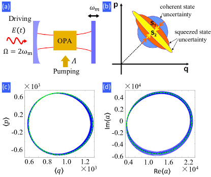
Figure 1: (Color online) (a) Sketch of the optomechanical setup. The optomechanical cavity that is driven by a periodically amplitude-modulated laser field contains an OPA, which is pumped by a laser of the frequency twice of the cavity resonance. See text for details. (b) Two-fold mechanical squeezing. The fluctuation in one quadrature of the mechanical mode, reduced to $S_{1}$ by the periodically amplitude-modulated cavity driving, is further shrunk to $S_{2}$ with the addition of the OPA driving. (c), (d) Phase space trajectories of the first moments of the mechanical mode for $t=[200\tau,360\tau]$ and optical mode for $t=[20\tau,160\tau]$ with numerical simulations (blue), and analytical approximations of the asymptotic orbits (green dash). Parameters are $\left(\kappa,\Delta_{0},g,\gamma_{m}\right)/\omega_{m}=\left(0.1,1.06,4\times 10^{-6},10^{-6}\right)$, $(E_{0},E_{+1},E_{-1})/\omega_{m}=(1.4,0.7,0.7)\times 10^{4}$, $\Lambda/\kappa=0.3$, $\theta=\pi$, $n_{a}=0$, $n_{m}=100$, and $\Omega=2\omega_{m}$.

In this paper, we study the quantum dynamics of an optical cavity that has a movable mirror and contains a degenerate OPA, and which is driven by a laser field with periodically modulated amplitude, as shown in Fig. 1(a). Our results reveal a cooperation-based enhancement of the squeezing in the fluctuation of the momentum or position of the cavity mirror. Both the parametric pump driving and periodically modulated cavity driving contribute to the reduction of the mechanical fluctuation. The resulting two-fold squeezing exceeds the squeezing that can be achieved solely by either of these two processes [see Fig. 1(b)]. The idea may be generalized to realize cooperation-based enhancement of other quantum effects in complex optomechanical systems, e.g., entanglement between two mechanical oscillators or entanglement between a light field and a mechanical oscillator Xuereb_pra2012 ; Farace_pra2012 .

II Theoretical model

We consider an optomechanical system where a degenerate OPA placed in a Fabry-Perot cavity of length $L$ and finesse $F$, with one fixed and partially transmitting mirror, and one movable and totally reflecting mirror Agarwal_pra2016 ; LvXY_PRL2015 . The movable mirror is treated as a quantum-mechanical harmonic oscillator with effective mass $m$, frequency $\omega_{m}$, and energy decay rate $\gamma_{m}$. The cavity mode of resonant frequency $\omega_{c}$ is driven by an external laser of the carrier frequency $\omega_{l}$ (along the cavity axis) with periodically modulated amplitude $E(t)=\sum_{n=-\infty}^{+\infty}E_{n}e^{-in\Omega t}$, where $\Omega=2\pi/\tau$ with $\tau>0$ being the modulation period, and the modulation coefficients $\{E_{n}\}$ are related to the power of the associated sidebands $\{P_{n}\}$ by $\left|E_{n}\right|=\sqrt{2\kappa P_{n}/\hbar\omega_{l}}$, with $\kappa=\pi c/(2FL)$ being the cavity decay rate due to photon leakage through the fixed mirror. The degenerate OPA in the optical cavity is pumped by a coherent field at frequency $2\omega_{p}$, which leads to the squeezing of cavity field Walls_book2007 ; NOTE , affecting the state of the movable cavity mirror through the optomechanical coupling. We denote the gain of the OPA by $\Lambda$ (which depends on the pumping intensity) and the phase of the pump driving as $\theta$. The total Hamiltonian of the system in the frame rotating at the laser frequency $\omega_{l}$ can be written as $(\hbar=1)$

$\displaystyle H=$ $\displaystyle\Delta_{0}a^{\dagger}a+\frac{\omega_{m}}{2}(p^{2}+q^{2})-ga^{\dagger}aq$
$\displaystyle+i\Lambda(e^{i\theta}a^{\dagger 2}e^{-i2\Delta_{p}t}-e^{-i\theta}a^{2}e^{i2\Delta_{p}t})$
$\displaystyle+i[E(t)a^{\dagger}-E^{*}(t)a].$ (1)

Here, $\Delta_{0}=\omega_{c}-\omega_{l}$, $\Delta_{p}=\omega_{p}-\omega_{l}$, $a$ and $a^{\dagger}$ are annihilation and creation operators of the cavity mode, $q$ and $p$ are the position and momentum operators for the movable mirror satisfying the standard canonical commutation relation $[q,\>p]=i$, and $g$=$x_{ZPF}\omega_{c}/L$ is the single-photon coupling strength between light and mechanical oscillator arising from the radiation pressure force, with $x_{ZPF}=\sqrt{\hbar/2m\omega_{m}}$ being the zero-point motion of the mechanical mode.

When the mechanical damping and cavity decay are included, the dissipative dynamics of the open system can be described by the following set of quantum Langevin equations (QLEs) Gardiner_book2004

$\displaystyle\dot{q}=$ $\displaystyle\omega_{m}p,$
$\displaystyle\dot{p}=$ $\displaystyle-\omega_{m}q-\gamma_{m}p+ga^{\dagger}a+\xi(t),$
$\displaystyle\dot{a}=$ $\displaystyle-(\kappa+i\text{$\Delta$}_{0})a+igaq+E(t)+2\Lambda e^{i\theta}a^{\dagger}e^{-i2\Delta_{p}t}$
$\displaystyle+\sqrt{2\kappa}a_{in}(t),$ (2)

where both the optical ($a_{in}$) and mechanical ($\xi$) noise operators have zero-mean value, and the nonzero correlation functions of $a_{in}$ are $\langle a_{in}^{\dagger}(t)a_{in}(t^{\prime})\rangle=n_{a}\delta(t-t^{\prime})$ and $\langle a_{in}(t)a_{in}^{\dagger}(t^{\prime})\rangle=(n_{a}+1)\delta(t-t^{\prime})$ with $n_{a}=[\exp(\hbar\omega_{c}/k_{B}T)-1]^{-1}$ being the thermal photon number and that of $\xi(t)$ is given by $\langle{\textstyle\xi(t)\xi(t^{\prime})\rangle}=\frac{\gamma_{m}}{\omega_{m}}\int\frac{d\omega}{2\pi}e^{-i\omega(t-t^{\prime})}\omega[1+\mathrm{coth}(\frac{\hbar\omega}{2k_{B}T})]$ Giovannetti_pra2001 ; Clerk_RMP2010 . For the specific case where the mechanical oscillator has a good quality factor $Q\equiv\omega_{m}/\gamma_{m}\gg 1$, $\xi(t)$ becomes delta-correlated $\langle\xi(t)\xi(t^{\prime})+\xi(t^{\prime})\xi(t)\rangle/2=\gamma_{m}(2n_{m}+1)\delta(t-t^{\prime})$ Benguria_PRL1981 ; Vitali_pra2007 , which corresponds to the Markovian process with $n_{m}=[\exp(\hbar\omega_{m}/k_{B}T)-1]^{-1}$ being the mean thermal excitation number in the mechanical mode.

III dynamics of the first moments of the optical and mechanical modes

Suppose that the external drivings are strong enough such that the intracavity photon number is much larger than 1, we can rewrite each Heisenberg operator as $O=\left\langle O(t)\right\rangle+\delta O$ ($O=q,\,p,\,a$), where $\delta O$ are quantum fluctuation operators with zero-mean values; and justify that $\left\langle a^{\dagger}(t)a(t)\right\rangle\simeq\left|\left\langle a(t)\right\rangle\right|^{2}$ and $\left\langle a(t)q(t)\right\rangle\simeq\left\langle a(t)\right\rangle\left\langle q(t)\right\rangle$ are valid approximations. Applying the standard linearization techniques to the QLEs (2) and setting $\Delta_{p}=\Omega/2$ for the consideration of mechanical squeezing, we thus obtain the equations for the first moments of the optical and mechanical modes

$\displaystyle\left\langle\dot{q}(t)\right\rangle=$ $\displaystyle\omega_{m}\left\langle p(t)\right\rangle,$
$\displaystyle\left\langle\dot{p}(t)\right\rangle=$ $\displaystyle-\omega_{m}\left\langle q(t)\right\rangle-\gamma_{m}\left\langle p(t)\right\rangle+g\left|\left\langle a(t)\right\rangle\right|^{2},$
$\displaystyle\left\langle\dot{a}(t)\right\rangle=$ $\displaystyle-(\kappa+i\Delta_{0})\left\langle a(t)\right\rangle+ig\left\langle a(t)\right\rangle\left\langle q(t)\right\rangle$
$\displaystyle+E(t)+2\Lambda e^{i\theta}\left\langle a(t)\right\rangle^{*}e^{-i\text{$\Omega$}t},$ (3)

and the linearized QLEs for the quantum fluctuations

$\displaystyle\delta\dot{q}$ $\displaystyle=$ $\displaystyle\omega_{m}\delta p,$
$\displaystyle\delta\dot{p}$ $\displaystyle=$ $\displaystyle-\omega_{m}\delta q-\gamma_{m}\delta p+g[\left\langle a(t)\right\rangle\delta a^{\dagger}+\left\langle a(t)\right\rangle^{*}\delta a]+\xi(t),$
$\displaystyle\delta\dot{a}$ $\displaystyle=$ $\displaystyle-(\kappa+i\Delta)\delta a+ig\left\langle a(t)\right\rangle\delta q+2\Lambda e^{i\theta}\delta a^{\dagger}e^{-i\Omega t}$ (4)
$\displaystyle+\sqrt{2\kappa}a_{in}(t),$

where $\Delta(t)=\Delta_{0}-g\left\langle q(t)\right\rangle$ is slightly modulated by the mechanical motion.

The phase space trajectories of the first moments $\left\langle O(t)\right\rangle$ can be found by simulating Eq. (3) for a set of typical parameters [see Figs. 1(c)-(d)] Groblacher_NatPhys2009 . When the system is far away from the optomechanical instabilities and multistabilities Ludwing_njp2008 , the semiclassical dynamics in the steady state will evolve toward a fixed orbit with a period being equal to the modulation period of the cavity driving $\tau$. Moreover, since the two nonlinear terms in Eq. (3) are both proportional to the coupling strength $g$, the asymptotic solutions of $\langle O(t)\rangle$ can then be expanded perturbatively in the powers of $g$ and in terms of the Fourier components for $g\ll\omega_{m}$ Mari_PRL2009 ; Mari_njp2012

$$\begin{array}[]{ccc}\left\langle O(t)\right\rangle&=&\stackrel{{\scriptstyle[}}{{j}}=0]{\infty}{\sum}\stackrel{{\scriptstyle[}}{{n}}=-\infty]{\infty}{\sum}\end{array}O_{n,\,j}e^{in\Omega t}g^{j}.$$ (5)

Substituting Eq. (5) into Eq. (3), we can then obtain the recursive formulas for the time-independent coefficients $O_{n,\,j}$ (see Appendix A). By truncating the series to the first terms with indexes $j=0,\,1,\,...,\,6$ and $n=-1,\,0,\,1$, we find that the analytical approximations for $\langle O(t)\rangle$ agree well with the numerical results shown in Fig. 1(c)-(d). Thus, the linearized dynamics can be evaluated with high accuracy for the effective optomechanical coupling simply written as

$$G(t)=g_{0}+g_{1}e^{-i\Omega t}+g_{-1}e^{i\Omega t},$$ (6)

where $g_{n}=|g_{n}|e^{i\phi_{n}}=\frac{1}{\sqrt{2}}\stackrel{{\scriptstyle[}}{{j}}=0]{\infty}{\sum}a_{-n,j}g^{j+1}$ with $n=-1,0,1$.

IV quantum fluctuations and Two-fold mechanical squeezing

To examine the effect of the modulation sidebands ($\sim e^{\pm i\Omega t}$), we introduce the mechanical annihilation and creation operators $\delta b=(\delta q+i\delta p)/\sqrt{2}$, $\delta b^{\dagger}=(\delta q-i\delta p)/\sqrt{2}$. Then, the QLEs for $\delta a$ and $\delta b$ are

$\displaystyle\delta\dot{a}$ $\displaystyle=$ $\displaystyle-i\Delta\delta a+iG(t)(\delta b^{\dagger}+\delta b)+2\Lambda e^{i\theta}\delta a^{\dagger}e^{-i\Omega t}-\kappa\delta a$
$\displaystyle+\sqrt{2\kappa}a_{in}(t),$
$\displaystyle\delta\dot{b}$ $\displaystyle=$ $\displaystyle-i\omega_{m}\delta b-\frac{\gamma_{m}}{2}(\delta b-\delta b^{\dagger})+i[G(t)\delta a^{\dagger}+G^{*}(t)\delta a]$ (7)
$\displaystyle+\sqrt{\gamma_{m}}b_{in}(t),$

with the mechanical noise operator $b_{in}$ satisfying $\text{$\langle$}b_{in}\rangle=0$, $\langle b_{in}^{\dagger}(t)b_{in}(t^{\prime})\rangle=n_{m}\delta(t-t^{\prime}),$ and $\langle b_{in}(t)b_{in}^{\dagger}(t^{\prime})\rangle=\left(n_{m}+1\right)\delta(t-t^{\prime}).$ We assume that the modulation frequency satisfies $\Omega=2\omega_{m}$ and the carrier frequency of the laser field driving the cavity is close to the anti-Stokes sideband, which leads to $\Delta=\Delta_{0}-g\langle q(t)\rangle\simeq\omega_{m}$ for weak optomechanical single-photon coupling. We further assume that the system is working in the resolved sideband regime: $\omega_{m}\gg\kappa$, and the driving fields are weak: $\omega_{m}\gg|g_{0}|,\,|g_{-1}|,\,|g_{1}|$. Under these conditions, if we substitute the slow varying fluctuation operators $\delta a(t)=\delta\tilde{a}(t)e^{-i\Delta t}$, $\delta b(t)=\delta\tilde{b}(t)e^{-i\omega_{m}t}$, $a_{in}(t)=\tilde{a}_{in}(t)e^{-i\Delta t}$ and $b_{in}(t)=\tilde{b}_{in}(t)e^{-i\omega_{m}t}$ into Eq. (7), the terms rotating at $\pm 2\omega_{m}$ and $\pm 4\omega_{m}$ can be ignored in the rotating wave approximation (RWA), which leads to

$\displaystyle\delta\dot{\tilde{a}}$ $\displaystyle=$ $\displaystyle ig_{0}\delta\tilde{b}+ig_{1}\delta\tilde{b}^{\dagger}+2\Lambda e^{i\theta}\delta\tilde{a}^{\dagger}-\kappa\delta\tilde{a}+\sqrt{2\kappa}\tilde{a}_{in}(t),$
$\displaystyle\delta\dot{\tilde{b}}$ $\displaystyle=$ $\displaystyle ig_{0}^{*}\delta\tilde{a}+ig_{1}\delta\tilde{a}^{\dagger}-\frac{\gamma_{m}}{2}\delta\tilde{b}+\sqrt{\gamma_{m}}\tilde{b}_{in}(t).$ (8)

Note that $\tilde{a}_{in}$ ($\tilde{b}_{in}$) has the same correlation function as $a_{in}$ ($b_{in}$). We then introduce the optical and mechanical quadratures with the tilded operators $\delta\tilde{x}=(\delta\tilde{a}+\delta\tilde{a}^{\dagger})/\sqrt{2}$, $\delta\tilde{y}=(\delta\tilde{a}-\delta\tilde{a}^{\dagger})/i\sqrt{2}$, $\delta\tilde{q}=(\delta\tilde{b}+\delta\tilde{b}^{\dagger})/\sqrt{2}$, $\delta\tilde{p}=(\delta\tilde{b}-\delta\tilde{b}^{\dagger})/i\sqrt{2}$, and the corresponding noise operators $\tilde{x}_{in}=(\tilde{a}_{in}+\tilde{a}_{in}^{\dagger})/\sqrt{2}$, $\tilde{y}_{in}=(\tilde{a}_{in}-\tilde{a}_{in}^{\dagger})/i\sqrt{2}$, $\tilde{q}_{in}=(\tilde{b}_{in}+\tilde{b}_{in}^{\dagger})/\sqrt{2}$, $\tilde{p}_{in}=(\tilde{b}_{in}-\tilde{b}_{in}^{\dagger})/i\sqrt{2}$, in terms of which the QLEs (8) can be rewritten as

$$\dot{U}t)=\tilde{M}U(t)+N(t),$$ (9)

where $U(t)=[\delta\tilde{q},\delta\tilde{p},\delta\tilde{x},\delta\tilde{y}]^{T}$, $N(t)=[\sqrt{\gamma_{m}}\tilde{q}_{in},\sqrt{\gamma_{m}}\tilde{p}_{in},\sqrt{2\kappa}\tilde{x}_{in},\sqrt{2\kappa}\tilde{y}_{in}]$, and

$$\tilde{M}=\left[\begin{array}[]{cccc}-\frac{\gamma_{m}}{2}&0&\mathrm{Im}g_{-}&-\mathrm{Re}g_{-}\\ 0&-\frac{\gamma_{m}}{2}&\mathrm{Re}g_{+}&\mathrm{Im}g_{+}\\ \mathrm{-Im}g_{+}&-\mathrm{Re}g_{-}&-\kappa+2\Lambda\cos\theta&2\Lambda\sin\theta\\ \mathrm{Re}g_{+}&-\mathrm{Im}g_{-}&2\Lambda\sin\theta&-\kappa-2\Lambda\cos\theta\end{array}\right]$$ (10)

with $g_{\pm}=g_{0}\pm g_{1}$. Note that the stability conditions derived from the Routh-Hurwitz criterion require the parametric gain to fulfill $\bar{\Lambda}\equiv 2\Lambda/\kappa<1$, the calculation of which is fussy and will not be shown here.

The mechanical squeezing can be measured by the variance of the tilded fluctuations $\left\langle\delta\tilde{q}^{2}\right\rangle$ and $\left\langle\delta\tilde{p}^{2}\right\rangle$, which are just the first two diagonal elements of the tilded covariance matrix $\tilde{V}_{i,j}(t)=[\langle U_{i}(t)U_{j}(t)\rangle+\langle U_{j}(t)U_{i}(t)\rangle]/2$. Using Eqs. (8)-(9), $\tilde{V}(t)$ in the steady state is dominated by the Lyapunov equation (see Appendix A)

$$\begin{array}[]{ccl}\tilde{M}\tilde{V}+\tilde{V}\tilde{M}^{T}&=&-D\end{array}$$ (11)

with $D=diag[0,\gamma_{m}(2n_{m}+1),\kappa(2n_{a}+1),\kappa(2n_{a}+1)]$. Eq. (11) can be analytically solved in the parameter regime with negligible mechanical damping $\gamma_{m}\approx 0$ and null thermal photon number $n_{a}=0$, leading to

$\displaystyle\left\langle\delta\tilde{q}^{2}\right\rangle$ $\displaystyle=S_{-}^{\Omega}-\bar{\text{$\Lambda$}}S_{-}^{\Lambda},\;\left\langle\delta\tilde{p}^{2}\right\rangle=S_{+}^{\Omega}+\bar{\text{$\Lambda$}}S_{+}^{\Lambda},$ (12)

where $S_{\mp}^{\Omega}=(|g_{0}|^{2}+|g_{1}|^{2}\mp 2|g_{0}||g_{1}|\cos\phi_{r})\mathcal{N}^{-1}$, $S_{\mp}^{\Lambda}=[|g_{0}|^{2}\cos\phi_{r,0}+|g_{1}|^{2}\cos\phi_{r,1}\mp 2|g_{0}||g_{1}|\cos(\frac{\phi_{r,0}+\phi_{r,1}}{2})]\mathcal{N}^{-1}$, $\mathcal{N}=2(1-\bar{\text{$\Lambda$}}^{2})(|g_{0}|^{2}-|g_{1}|^{2}),$ with $\phi_{r}\equiv\phi_{1}-\phi_{0}$, $\phi_{r,0}\equiv\theta-2\phi_{0}$, and $\phi_{r,1}\equiv\theta-2\phi_{1}$. Eq. (12) shows that, under the interplay between the periodic cavity driving and the parametric interaction, the fluctuations of the position and momentum of the mechanical oscillator strongly depend on the phase matching condition. To clarify the underlying physics clearly, we assume $\phi_{r}=\pi,$ $\phi_{r,0}=\pi$ and $\phi_{r,1}=-\pi$, then the variance of the position and momentum fluctuations reduce to

$\displaystyle\left\langle\delta\tilde{q}^{2}\right\rangle$ $\displaystyle=$ $\displaystyle\frac{1}{2}\frac{1+|\frac{g_{1}}{g_{0}}|}{1-|\frac{g_{1}}{g_{0}}|}(1-\bar{\text{$\Lambda$}})^{-1},$ (13)
$\displaystyle\left\langle\delta\tilde{p}^{2}\right\rangle$ $\displaystyle=$ $\displaystyle\frac{1}{2}\frac{1-|\frac{g_{1}}{g_{0}}|}{1+|\frac{g_{1}}{g_{0}}|}(1+\bar{\text{$\Lambda$}})^{-1},$ (14)

which reveal that the mechanical mode is squeezed in momentum (i.e. $\left\langle\delta\tilde{p}^{2}\right\rangle<0.5$). Alternatively, the position squeezing can be achieved by setting $\phi_{r}=0,$ $\phi_{r,0}=0$ and $\phi_{r,1}=0$. More importantly, Eq. (14) shows that the cooperation between the two driving fields results in a two-fold squeezing: The coefficient ($1-|\frac{g_{1}}{g_{0}}|)/(1+|\frac{g_{1}}{g_{0}}|$) describes the squeezing effect produced by the periodically modulated cavity driving, while $(1+\bar{\text{$\Lambda$}})^{-1}$ corresponds to the effect associated with the parametric driving.

Refer to caption
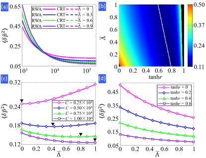
Figure 2: (Color online) (a) $\langle\delta\tilde{p}^{2}\rangle$ versus cooperativity parameter $C$ under RWA [Eq. (18)] and with counter-rotating terms (CRT) included [Eq. (7)] for, $|g_{1}|/|g_{0}|=0.6$, $|g_{-1}|/|g_{1}|=0.3$, and a set of OPA gains $\bar{\Lambda}$. (b) $\langle\delta\tilde{p}^{2}\rangle$ versus $\bar{\Lambda}$ and $\tanh r$ for $C=1.0\times 10^{4}$. The black region indicates that the mechanical oscillator is not squeezed. The white line denotes the optimal parametric gain $\bar{\Lambda}$ with which the momentum squeezing reaches its maximum for a given $\tanh r$. (c) $\langle\delta\tilde{p}^{2}\rangle$ versus $\bar{\Lambda}$ for different cooperativity parameters $C$ with $\tanh r=0.6$. The black arrows indicate the optimal squeezing. (d) $\langle\delta\tilde{p}^{2}\rangle$ versus $\bar{\Lambda}$ for different modulations of the cavity driving with $C=5\times 10^{4}$. The makers in (c)-(d) indicate the numerical counterpart via the Fourier transformation, see Appendix C. In all figures other parameters are $\kappa/\omega_{m}=0.1$, $n_{a}=0$, $n_{m}=100$, $\gamma_{m}/\omega_{m}=10^{-6}$.

The two-fold mechanical squeezing can be further understood by introducing the Bogoliubov mode defined as $\delta B\equiv\delta\tilde{b}\cosh r+e^{i\phi_{r}}\delta\tilde{b}^{\dagger}\sinh r$ with $\tanh r=|g_{1}|/|g_{0}|$ Pirkkalainen_PRL2015 ; Kron_pra2013 , which evolves according to the QLEs

$\displaystyle\delta\dot{B}$ $\displaystyle=$ $\displaystyle ig_{B}^{*}\delta\tilde{a}-\frac{\gamma_{m}}{2}\delta B+\sqrt{\gamma_{m}}B_{in},$
$\displaystyle\delta\dot{\tilde{a}}$ $\displaystyle=$ $\displaystyle-\kappa\delta\tilde{a}+ig_{B}\delta B+2\text{$\Lambda$}e^{i\theta}\delta\tilde{a}^{\dagger}+\sqrt{2\kappa}\tilde{a}_{in},$ (15)

with $g_{B}=\sqrt{|g_{0}|^{2}-|g_{1}|^{2}}e^{i\phi_{0}}$. Since the vacuum state of the Bogoliubov mode corresponds to a squeezed state, the noise input $B_{in}$ for $\delta B$ has zero mean and the nonzero correlation functions $\langle B_{in}^{\dagger}(t)B_{in}(t^{\prime})\rangle=[(n_{m}+1)\sinh^{2}r+n_{m}\cosh^{2}r]\delta(t-t^{\prime})$ and $\langle B_{in}(t)B_{in}^{\dagger}(t^{\prime})\rangle=[(n_{m}+1)\cosh^{2}r+n_{m}\sinh^{2}r]\delta(t-t^{\prime}).$ By applying the adiabatic approximation for $\kappa\gg|g_{B}|$ (i.e. $\delta\dot{\tilde{a}}$=0) Agarwal_pra2016 , and considering the phase matching condition ($\phi_{r,0}=\pi$) for momentum squeezing, we find that the variance of the quadrature $\delta p_{B}=\frac{1}{\sqrt{2}i}(\delta B-\delta B^{\dagger})$ in the steady state reads (see Appendix B)

$\displaystyle\langle\delta p_{B}^{2}$ $\displaystyle\rangle=$ $\displaystyle\frac{\kappa\gamma_{m}(1+\bar{\text{$\Lambda$}})}{4\left|g_{B}\right|^{2}}(2\sinh^{2}r+1)(2n_{m}+1)$ (16)
$\displaystyle+\frac{1}{2(1+\bar{\text{$\Lambda$}})}(2n_{a}+1).$

For $\phi_{r}=\pi$, the variance of the momentum fluctuation for the original mechanical mode has a simply analytical form

$\displaystyle\langle\delta\tilde{p}^{2}\rangle$ $\displaystyle=$ $\displaystyle(\cosh r-\sinh r)^{2}\langle\delta p_{B}^{2}\rangle,$ (17)

which is exactly the result of Eq. (14) for $\gamma_{m}=0$, $n_{a}=0$. This result can be roughly explained as follows: The periodically modulated cavity driving produces a squeezing effect on the momentum fluctuation of the mechanical mode, which mathematically corresponds to converting the normal mechanical mode into the Bogoliubov mode through a unitary transformation equivalent to a squeezed operator. As a consequence, the “momentum” fluctuation of the Bogoliubov mode at the “vacuum” level corresponds to the normal momentum fluctuation below the vacuum level ($\left\langle\delta\tilde{p}^{2}\right\rangle<0.5$). The parametric driving further reduces the “momentum” fluctuation of the Bogoliubov mode below the “vacuum” level, resulting in a second squeezing effect.

V The effect of mechanical damping and experimental feasibility

Considering the effect of the mechanical damping $\gamma_{m}\neq 0$, the variances of the fluctuations $\left\langle\delta\tilde{q}^{2}\right\rangle$ and $\left\langle\delta\tilde{p}^{2}\right\rangle$ can again be calculated by the Lyapunov equation (11). As an example, when the phases $\phi_{0}=0$, $\phi_{r}=\pi$ and $\theta=\pi$ are set and the cooperativity parameter $C=4|g_{0}|^{2}/(\kappa\gamma_{m})$ is large so that $\tilde{C}\equiv C(1-\tanh^{2}r)\gg 2(1+\bar{\Lambda})$, the variance of the momentum is approximately given by

$\displaystyle\left\langle\delta\tilde{p}^{2}\right\rangle$ $\displaystyle\approx$ $\displaystyle\frac{(\cosh r-\sinh r)^{2}}{2(1+\bar{\Lambda})}$ (18)
$\displaystyle+(2n_{m}+1)[\frac{1+\bar{\Lambda}}{\tilde{C}}+\frac{\gamma_{m}}{4\kappa(1+\bar{\Lambda})}].$

which agrees well with its numerical counterpart obtained by simulation of Eq. (7), as shown in Fig. 2(a). For $|g_{1}|\simeq|g_{0}|$ (corresponding to $\tanh r\rightarrow 1$), the effective coupling between the Bogoliubov mode and the cavity mode becomes negligible, and $\left\langle\delta\tilde{p}^{2}\right\rangle\simeq n_{m}+\frac{1}{2}$ is mainly determined by the thermal occupation of the mechanical mode with $\gamma_{m}\ll\kappa$, implying that the mechanical mode is not squeezed [see Fig. 2(b)] Woll_Sci2015 . In this case, the self-cooling of the mechanical oscillator through the photon-phonon sideband coupling is suppressed Gigan_Nature2006 ; Kleckner_Nature2006 ; Marquardt_PRL2007 , therefore, the mechanical oscillator may stay far away from the ground state Kron_pra2013 ; Schonburg_pra2016 . Generally, there exists an optimal squeezing for $\langle\delta\tilde{p}^{2}\rangle$ corresponding to the best efficiency of the cooperation between the two driving fields, which can be readily found by setting $\textrm{d}\langle\delta\tilde{p}^{2}\rangle/\textrm{d}\bar{\Lambda}=0$ for an appropriate amplitude modulation $|g_{1}|/|g_{0}|$ (i.e. a given $\tanh r$). For $\tilde{C}\gg 1$, $\left\langle\delta\tilde{p}^{2}\right\rangle$ reaches its minimum when the optimal parametric gain satisfies $\bar{\Lambda}_{opt}=\frac{\text{$\eta$}}{2}\text{(}1+\sqrt{1+\frac{\tilde{C}}{\eta}})-1$ with $\eta=\frac{(\cosh r-\sinh r)^{2}}{n_{m}+\frac{1}{2}}+\frac{\gamma_{m}}{\kappa},$ which is indicated in Fig. 2(b). Note that an effective cooperation implies a non-negative $\bar{\Lambda}_{opt}$, which imposes a threshold of $\tilde{C}_{thr}=4(\eta^{-1}-1)$ on $\tilde{C}$, namely $\tilde{C}>\tilde{C}_{thr}$. In addition, the stability condition $\bar{\Lambda}_{opt}<1$ requires $\tilde{C}<\tilde{C}_{ins}$ with $\tilde{C}_{ins}=8(2\eta^{-1}-1)$, beyond which the best cooperation efficiency always appears at $\bar{\Lambda}_{opt}\rightarrow 1$, in vicinity of instability, see Fig. 2(c) for the example of $\tanh r=0.6$, where we find $\tilde{C}_{thr}\approx 1.6\times 10^{3}$ ($C_{thr}\approx 2.5\times 10^{3}$) and $\tilde{C}_{ins}\approx 6.4\times 10^{3}$ ($C_{ins}\approx 10^{4}$).

Considering the set of experimentally feasible parameters Groblacher_NatPhys2009 : $L=25$ mm, $F=1.4\times 10^{4}$, $\omega_{m}/2\pi=1$ MHz, $Q=10^{6}$, $m=150$ ng, $T=5$ mK and the power of the carrier component $P_{0}=1$ mW of the driving laser ($\lambda=1064$ nm), we show in Fig. 2(d) that the degree of squeezing for the mechanical momentum with $C=5\times 10^{4}$ and thermal occupation $n_{m}=100$ is monotonically improved as the dimensionless parametric gain $\bar{\Lambda}$ increases for $\tanh r=0$, $0.2$, $0.4$, $0.6$ due to $\tilde{C}>\tilde{C}_{ins}$. Under this condition, the momentum fluctuation is reduced from 0.219 (3.57 dB) to 0.117 (6.29 dB) for $\tanh r=0.4$, and from 0.132 (5.79 dB) to 0.0756 (8.21 dB) for $\tanh r=0.6$ as the parametric gain $\bar{\Lambda}$ is increased from 0 to the optimal value 0.99. The momentum squeezing can be further increased for a larger $C/n_{m}$ ratio (the so-called quantum cooperativity) under the best efficiency of the two-field cooperation. Our results clearly show that, with suitable choice of the system parameters, both the cavity driving and parametric interaction significantly contribute to the reduction of the mechanical momentum fluctuation; their cooperation is important for realization of a strong mechanical squeezing.

VI Conclusion

In summary, we have shown that the parametric driving and the periodically modulated cavity driving, simultaneously applied to a cavity optomechanical system, can result in a two-fold squeezing effects on the mechanical oscillator. This enables implementation of strong squeezing for a macroscopic oscillator, which exceeds the result that is solely produced by either of these two drivings. Our results show that different physical processes, each producing a weak quantum effect, can cooperate to enhance the quantum effect. Our idea can be generalized to more complex optomechanical systems to realize two-fold two-mode squeezing, offering a possibility to produce strong mechanical-mechanical or optomechanical entanglement that can exceed the bound imposed by present methods.

Acknowledgements.
This work was supported by the National Natural Science Foundation of China under Grants No. 11774058 and No. 11774024, and the Natural Science Foundation of Fujian Province under Grant No. 2017J01401.

Appendix A Periodic motion and quantum dynamics of the mechanical oscillator in the steady state

The time-independent coefficients $O_{n,\,j}$ in the Fourier expansion of $\left\langle O(t)\right\rangle$ ($O=q,p,a$) given by Eq. (5) can be found by substituting Eq. (5) into Eq. (3), leading to the following recursive formulas

$\displaystyle p_{n,0}=0,\;q_{n,0}=0,$ (19)
$\displaystyle a_{n,0}$ $\displaystyle=$ $\displaystyle\frac{\left[\kappa-i\left(\Delta_{0}-(n+1)\Omega\right)\right]E_{-n}+2\Lambda e^{i\theta}E_{n+1}}{\left[\kappa-i\left(\Delta_{0}-(n+1)\Omega\right)\right]\left[\kappa+i\left(\Delta_{0}+n\Omega\right)\right]-4\Lambda^{2}},$

corresponding to the zeroth-order perturbation with respect to $g$, and with $j>0$,

$\displaystyle q_{n,j}$ $\displaystyle=$ $\displaystyle\omega_{m}\stackrel{{\scriptstyle[}}{{k}}=0]{j-1}{\sum}\stackrel{{\scriptstyle[}}{{m}}=-\infty]{\infty}{\sum}\frac{a_{m,k}^{*}a_{n+m,j-k-1}}{\omega_{m}^{2}-(n\Omega)^{2}+i\gamma_{m}n\Omega},$
$\displaystyle p_{n,j}$ $\displaystyle=$ $\displaystyle\frac{in\Omega}{\omega_{m}}q_{n,j},$ (20)
$\displaystyle a_{n,j}$ $\displaystyle=$ $\displaystyle\frac{2\Lambda e^{i\theta}a_{-n-1,j}^{*}}{\kappa+i(\Delta_{0}+n\Omega)}+i\stackrel{{\scriptstyle[}}{{k}}=0]{j-1}{\sum}\stackrel{{\scriptstyle[}}{{m}}=-\infty]{\infty}{\sum}\frac{a_{m,k}q_{n-m,j-k-1}}{\kappa+i(\Delta_{0}+n\Omega)}.$

Using Eq. (19) and (20), the quantum dynamics of the mechanical oscillator can be studied through the linearized QLEs (4).

We introduce the amplitude and phase quadratures of the cavity mode as $\delta x=(\delta a+\delta a^{\dagger})/\sqrt{2}$, $\delta y=(\delta a-\delta a^{\dagger})/i\sqrt{2}$ and the analogous input quantum noise quadratures as $\delta x_{in}=(\delta a_{in}+\delta a_{in}^{\dagger})/\sqrt{2}$, $\delta y_{in}=(\delta a_{in}-\delta a_{in}^{\dagger})/i\sqrt{2}$ for convenience. Then the time-dependent equations of motion for the quantum fluctuations $u(t)=[\delta q,\delta p,\delta x,\delta y]^{T}$ arise as

$$\dot{u}(t)=M(t)u(t)+n(t),$$ (21)

with the drift matrix

$$M(t)=\left[\begin{array}[]{cccc}0&\omega_{m}&0&0\\ -\omega_{m}&-\gamma_{m}&2G_{x}(t)&2G_{y}(t)\\ -2G_{y}(t)&0&-\kappa+2\Lambda\cos\bar{\theta}&\Delta-2\Lambda\sin\bar{\theta}\\ 2G_{x}(t)&0&-\Delta-2\Lambda\sin\bar{\theta}&-\kappa-2\Lambda\cos\bar{\theta}\end{array}\right],$$

and the diffusion $n(t)=[0,\xi(t),\sqrt{2\kappa}\delta x_{in},\sqrt{2\kappa}\delta y_{in}]^{T}$ being the noise sources. Here $\bar{\theta}=\Omega t-\theta$, and $G_{x}$, $G_{y}$ are real part and imaginary part of the effective optomechanical coupling $G(t)\equiv g\left\langle a(t)\right\rangle/\sqrt{2}$. If all the eigenvalues of the matrix $M(t)$ have negative real parts at any time (i.e. the Routh-Hurwitz criterion) pra1987_Dejesus , the system will be in stable in the steady state. On the other hand, since the system in the steady state will evolve into an asymptotic Gaussian state for a Gaussian-typed of noise RMP2012_Weed , we can then characterize the second moments of the quadratures of the asymptotic state through the covariance matrix (CM) $V(t)$, with the matrix elements being

$$\begin{array}[]{ccc}V_{k,l}(t)&=&\langle u_{k}(t)u_{l}^{\dagger}(t)+u_{l}^{\dagger}(t)u_{k}(t)\rangle/2.\end{array}$$ (22)

From Eqs. (21) and (22), we can easily derive a linear differential equation governing the evolution of the CM $V(t)$

$$\begin{array}[]{ccc}\dot{V}(t)&=&M(t)V(t)+V(t)M^{T}(t)+D,\end{array}$$ (23)

where $M(t)^{T}$ is the transpose matrix of $M(t)$, and $\begin{array}[]{ccc}D&=&diag[0,\gamma_{m}(2n_{m}+1),\kappa(2n_{a}+1),\kappa(2n_{a}+1)]\end{array}$ is a diagonal noise correlations matrix, defined by $\delta(t-t^{\prime})D_{k,l}=\langle n_{k}(t)n_{l}^{\dagger}(t^{\prime})+n_{l}^{\dagger}(t^{\prime})n_{k}(t)\rangle/2$. The first two diagonal elements $V_{11}(t)=\left\langle\delta q(t)^{2}\right\rangle$, $V_{22}(t)=\left\langle\delta p(t)^{2}\right\rangle$ of $V(t)$ represent the variances of the fluctuations in the mechanical position and momentum, and the last two terms $V_{33}(t)=\left\langle\delta x(t)^{2}\right\rangle$, $V_{44}(t)=\left\langle\delta y(t)^{2}\right\rangle$ represent the variances of the fluctuations in the amplitude and phase of the cavity mode. The mechanical oscillator is position- or momentum-squeezed if either $\left\langle\delta q(t)^{2}\right\rangle<1/2$ or $\left\langle\delta p(t)^{2}\right\rangle<1/2$ in the steady state. The degree of the squeezing can be expressed in the dB unit, which can be calculated by $-10\log_{10}\frac{\left\langle\delta o(t)^{2}\right\rangle}{\left\langle\delta o(t)^{2}\right\rangle_{vac}}$ (or $o=p,\,q$), with $\left\langle\delta q(t)^{2}\right\rangle_{vac}=\left\langle\delta p(t)^{2}\right\rangle_{vac}=1/2$ being the position and momentum variances of the vacuum state.

Refer to caption
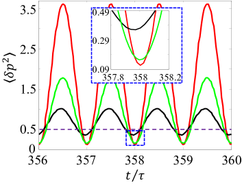
Figure 3: (Color online) Variances of the mechanical momentum fluctuation $\left\langle\delta p(t)^{2}\right\rangle$ versus rescaled time $t/\tau$ for the modulation sidebands driving amplitudes $E_{\pm 1}$ and the parametric gain $\Lambda$ being (i) $E_{\pm 1}=0$, $\Lambda$/$\kappa$=0.3 (black), (ii) $E_{\pm 1}/\omega_{m}=0.7\times 10^{4}$, $\Lambda/\kappa=0$ (green), (iii) $E_{\pm 1}/\omega_{m}=0.7\times 10^{4}$, $\Lambda$/$\kappa$=0.3 (red). The dash line represents the momentum variance of the vacuum state $\left\langle\delta p(t)^{2}\right\rangle_{vac}=0.5$. Other parameters are the same as in Fig. 1(c),(d).

Recalling that the asymptotic behavior of the first moments of the mechanical mode and the cavity mode is $\tau=2\pi/\Omega$ periodic in the steady state, then we can find that the drift matrix $M(t)$, which is related to $\langle a(t)\rangle$ and $\langle q(t)\rangle$, satisfies $M(t+\tau)=M(t)$ and therefore $V(t+\tau)=V(t)$ according to the Floquet theory www_Teschl . By solving the evolutional equation (23) of the CM $V(t)$, we have calculated the time-dependent variances of the mechanical momentum $\left\langle\delta p(t)^{2}\right\rangle$ for the optomechanical system with (i) OPA, (ii) periodic driving, and (iii) both OPA and periodic driving, as shown in Fig.3. It has been realized that the cavity solely pumped by parametric interaction (with $E_{\pm 1}=0$) Agarwal_pra2016 and solely modulated by periodic driving ($\Lambda=0$) Mari_PRL2009 can both lead to mechanical squeezing, the degree of which (corresponding to the minimum of $\left\langle\delta p(t)^{2}\right\rangle$) can reach 1.44 dB ($\left\langle\delta p(t)^{2}\right\rangle_{min}=0.359$) for $\Lambda/\kappa=0.3$, and 5.13 dB ($\left\langle\delta p(t)^{2}\right\rangle_{min}=0.153$) for $E_{\pm 1}/\omega_{m}=0.7\times 10^{4}$, respectively. However, we note that, by combining OPA and periodic driving simultaneously, the mechanical squeezing will be greatly enhanced, the degree of momentum squeezing can achieve as large as 6.31 dB ($\left\langle\delta p(t)^{2}\right\rangle_{min}=0.117$), which is far beyond the 3 dB limit, required for ultrahigh-precision measurements.

Appendix B The steady-state “momentum” fluctuation of the Bogoliubov mode

The QLEs (15) can be solved in the adiabatic approximation under the condition of $\kappa\gg|g_{B}|$. For this purpose, we rewrite the equations of motion for $\delta\tilde{a}$ and $\delta\tilde{a}^{\dagger}$:

$\displaystyle\delta\dot{\tilde{a}}$ $\displaystyle=$ $\displaystyle-\kappa\delta\tilde{a}+ig_{B}\delta B+2\text{$\Lambda$}e^{i\theta}\delta\tilde{a}^{\dagger}+\sqrt{2\kappa}\tilde{a}_{in},$
$\displaystyle\delta\dot{\tilde{a}}^{\dagger}$ $\displaystyle=$ $\displaystyle-\kappa\delta\tilde{a}^{\dagger}-ig_{B}^{*}\delta B^{\dagger}+2\text{$\Lambda$}e^{-i\theta}\delta\tilde{a}+\sqrt{2\kappa}\tilde{a}_{in}^{\dagger}.$ (24)

Setting $\delta\dot{\tilde{a}}=\delta\dot{\tilde{a}}^{\dagger}=0$ and $\theta-2\phi_{0}=0$, it is readily to find

$\displaystyle\delta\tilde{a}$ $\displaystyle=$ $\displaystyle i\frac{g_{B}}{\kappa(1-\bar{\text{$\Lambda$}}^{2})}(\delta B+\text{$\bar{\text{$\Lambda$}}$}\delta B^{\dagger})$ (25)
$\displaystyle+\frac{\sqrt{2\kappa}}{\kappa(1-\bar{\text{$\Lambda$}}^{2})}(\tilde{a}_{in}+\text{$\bar{\text{$\Lambda$}}$}e^{i\theta}\tilde{a}_{in}^{\dagger}).$

Inserting Eq. (25) into $\delta\dot{B}=ig_{B}^{*}\delta\tilde{a}-\frac{\gamma_{m}}{2}\delta B+\sqrt{\gamma_{m}}B_{in},$ we have

$\displaystyle\delta\dot{B}$ $\displaystyle=$ $\displaystyle-\frac{|g_{B}|^{2}}{\kappa(1-\bar{\text{$\Lambda$}}^{2})}(\delta B+\bar{\text{$\Lambda$}}\delta B^{\dagger})+\sqrt{\gamma_{m}}B_{in}$ (26)
$\displaystyle+\frac{ig_{B}^{*}\sqrt{2\kappa}}{\kappa(1-\bar{\text{$\Lambda$}}^{2})}(\delta\tilde{a}_{in}+\bar{\text{$\Lambda$}}e^{i\theta}\delta\tilde{a}_{in}^{\dagger}).$

Here, the term $\gamma_{m}$ in the coefficient of $\delta B$ is safely ignored in our parameter regime. Then the equation of motion for the “momentum” of the Bogoliubov mode $\delta p_{B}$ is given by

$\displaystyle\delta\dot{p}_{B}$ $\displaystyle=$ $\displaystyle-\frac{|g_{B}|^{2}}{\kappa(1+\bar{\text{$\Lambda$}})}\delta p_{B}+d(t)+v(t),$ (27)

where $d(t)=\frac{1}{i}\sqrt{\frac{\gamma_{m}}{2}}(B_{in}-B{}_{in}^{\dagger})$ and $v(t)=\frac{g_{B}^{*}\sqrt{\kappa}}{\kappa(1+\bar{\text{$\Lambda$}})}(\tilde{a}_{in}-\tilde{a}_{in}^{\dagger})e^{i\theta}$, whose correlation functions are $\langle d(t)d(t^{\prime})\rangle=\frac{\gamma_{m}}{2}(2\sinh^{2}r+1)(2n_{m}+1)\delta(t-t^{\prime})$ and $\langle v(t)v(t^{\prime})\rangle=\frac{|g_{B}|^{2}}{\kappa(1+\bar{\text{$\Lambda$}})^{2}}(2n_{a}+1)\delta(t-t^{\prime})$, respectively. Based on these equations, we obtain the equation for $\left\langle\delta p_{B}^{2}\right\rangle$ as

$\displaystyle\frac{\partial\langle\delta p_{B}^{2}\rangle}{\partial t}$ $\displaystyle=$ $\displaystyle-\frac{2|g_{B}|^{2}}{\kappa(1+\bar{\text{$\Lambda$}})}\langle\delta p_{B}^{2}\rangle+\frac{|g_{B}|^{2}}{\kappa(1+\bar{\text{$\Lambda$}})^{2}}(2n_{a}+1)$ (28)
$\displaystyle+\frac{\gamma_{m}}{2}(2\sinh^{2}r+1)(2n_{m}+1).$

As a result, the steady-state “momentum” fluctuation of the Bogoliubov mode can be solved by setting $\frac{\partial\langle\delta p_{B}^{2}\rangle}{\partial t}=0$, giving rise to Eq. (16) in the main text.

Appendix C Optomechanical squeezing in the rotating wave approximation

Taking the Fourier transform of Eq. (9) by using $f(t)=\frac{1}{2\pi}\intop_{-\infty}^{+\infty}f(\omega)e^{-i\omega t}d\omega$ and $f^{\dagger}(t)=\frac{1}{2\pi}\int_{-\infty}^{+\infty}f^{\dagger}(-\omega)e^{-i\omega t}d\omega$, we obtain the position and momentum fluctuations of the movable mirror in the frequency domain, i.e.

$$\begin{array}[]{ccc}\delta\tilde{q}(\omega)&=&A_{1}(\omega)\tilde{x}_{in}(\omega)+B_{1}(\omega)\tilde{y}_{in}\\ &&+E_{1}(\omega)\tilde{q}_{in}(\omega)+F_{1}(\omega)\tilde{p}_{in},\\ \delta\tilde{p}(\omega)&=&A_{2}(\omega)\tilde{x}_{in}(\omega)+B_{2}(\omega)\tilde{y}_{in}\\ &&+E_{2}(\omega)\tilde{q}_{in}(\omega)+F_{2}(\omega)\tilde{p}_{in},\end{array}$$ (29)

where

$$\begin{array}[]{ccl}A_{1}(\omega)&=&-\frac{\sqrt{2\kappa}i}{d(\omega)}\{[\Lambda(\alpha_{0}-\alpha_{1})+iu(\omega)\mathrm{Im}(g_{0}-g_{1})]v(\omega)\\ &&+i(\left|g_{0}\right|^{2}-\left|g_{1}\right|^{2})\mathrm{Im}(g_{0}-g_{1})\},\\ B_{1}(\omega)&=&\frac{\sqrt{2\kappa}}{d(\omega)}\{[\Lambda(\beta_{0}-\beta_{1})-u(\omega)\mathrm{Re}(g_{0}-g_{1})]v(\omega)\\ &&-(\left|g_{0}\right|^{2}-\left|g_{1}\right|^{2})\mathrm{Re}(g_{0}-g_{1})\},\\ E_{1}(\omega)&=&\frac{\sqrt{\gamma_{m}}}{d(\omega)}\{[u(\omega)^{2}-4\Lambda^{2}]v(\omega)\\ &&+(\left|g_{0}\right|^{2}-\left|g_{1}\right|^{2})u(\omega)+\Lambda(\Gamma_{0}-\Gamma_{1})\},\\ F_{1}(\omega)&=&\frac{\sqrt{\gamma_{m}}}{d(\omega)}i\Lambda[(g_{0}-g_{1})^{2}e^{-i\theta}-(g_{0}^{*}-g_{1}^{*})^{2}e^{i\theta}],\\ A_{2}(\omega)&=&\frac{\sqrt{2\kappa}}{d(\omega)}\{[\Lambda(\beta_{0}+\beta_{1})+u(\omega)\mathrm{Re}(g_{0}+g_{1})]v(\omega)\\ &&+(\left|g_{0}\right|^{2}-\left|g_{1}\right|^{2})\mathrm{Re}(g_{0}+g_{1})\},\\ B_{2}(\omega)&=&\frac{\sqrt{2\kappa}i}{d(\omega)}\{[\Lambda(\alpha_{0}+\alpha_{1})-iu(\omega)\mathrm{Im}(g_{0}+g_{1})]v(\omega)\\ &&-i(\left|g_{0}\right|^{2}-\left|g_{1}\right|^{2})\mathrm{Im}(g_{0}+g_{1})\},\\ E_{2}(\omega)&=&\frac{\sqrt{\gamma_{m}}}{d(\omega)}i\Lambda[(g_{0}+g_{1})^{2}e^{-i\theta}-(g_{0}^{*}+g_{1}^{*})^{2}e^{i\theta}],\\ F_{2}(\omega)&=&\frac{\sqrt{\gamma_{m}}}{d(\omega)}\{[u(\omega)^{2}-4\Lambda^{2}]v(\omega)\\ &&+(\left|g_{0}\right|^{2}-\left|g_{1}\right|^{2})u(\omega)-\Lambda(\Gamma_{0}-\Gamma_{1})\},\end{array}$$ (30)

with $\alpha_{0}=g_{0}e^{-i\theta}-g_{0}^{*}e^{i\theta}$, $\alpha_{1}=g_{1}e^{-i\theta}-g_{1}^{*}e^{i\theta}$ , $\beta_{0}=g_{0}e^{-i\theta}+g_{0}^{*}e^{i\theta}$, $\beta_{1}=g_{1}e^{-i\theta}+g_{1}^{*}e^{i\theta}$ , $\Gamma_{0}=g_{0}^{2}e^{-i\theta}+g_{0}^{*2}e^{i\theta}$, $\Gamma_{1}=g_{1}^{2}e^{-i\theta}+g_{1}^{*2}e^{i\theta}$, $u(\omega)=\frac{\gamma_{m}}{2}-i\omega$, $v(\omega)=\kappa-i\omega$ and

$$\begin{array}[]{ccl}d(\omega)&=&[u(\omega)v(\omega)+(\left|g_{0}\right|^{2}-\left|g_{1}\right|^{2})]^{2}-4\Lambda^{2}v(\omega)^{2}.\end{array}$$ (31)

The first two terms in $\delta\tilde{q}(\omega)$ and $\delta\tilde{p}(\omega)$ originate from the radiation pressure contribution, and the last two terms are from the thermal noise contribution. Without optomechanical coupling ($g_{0}=g_{1}=0$), the mechanical mode subjected to the purely thermal noise will make quantum Brownian motion leading to $\delta\tilde{q}(\omega)=$ $\frac{\sqrt{\gamma_{m}}}{\frac{\gamma_{m}}{2}-i\omega}\tilde{q}_{in}$ and $\delta\tilde{p}(\omega)=$ $\frac{\sqrt{\gamma_{m}}}{\frac{\gamma_{m}}{2}-i\omega}\tilde{p}_{in}$. The expressions of the spectra for the position and momentum fluctuations of the mechanical mode are ($Z=\tilde{q},\,\tilde{p}$)

$$\begin{array}[]{ccl}S_{Z}(\omega)&=&\frac{1}{4\pi}\int_{-\infty}^{+\infty}d\omega^{\prime}e^{-i(\omega^{\prime}+\omega)t}\\ &&\times[\left\langle\delta Z(\omega)\delta Z(\omega^{\prime})\right\rangle+\left\langle\delta Z(\omega^{\prime})\delta Z(\omega)\right\rangle],\end{array}$$ (32)

which can be solved by using the correlation functions of the noise sources in the frequency domain Agarwal_pra2016

$$\begin{array}[]{cll}\left\langle\tilde{q}_{in}(\omega)\tilde{q}_{in}(\omega^{\prime})\right\rangle&=&\left\langle\tilde{p}_{in}(\omega)\tilde{p}_{in}(\omega^{\prime})\right\rangle\\ &=&(n_{m}+\frac{1}{2})2\pi\delta(\omega+\omega^{\prime}),\\ \left\langle\tilde{q}_{in}(\omega)\tilde{p}_{in}(\omega^{\prime})\right\rangle&=&-\left\langle\tilde{p}_{in}(\omega)\tilde{q}_{in}(\omega^{\prime})\right\rangle\\ &=&\frac{i}{2}2\pi\delta(\omega+\omega^{\prime}),\\ \left\langle\tilde{x}_{in}(\omega)\tilde{x}_{in}(\omega^{\prime})\right\rangle&=&\left\langle\tilde{y}_{in}(\omega)\tilde{y}_{in}(\omega^{\prime})\right\rangle\\ &=&(n_{a}+\frac{1}{2})2\pi\delta(\omega+\omega^{\prime}),\\ \left\langle\tilde{x}_{in}(\omega)\tilde{y}_{in}(\omega^{\prime})\right\rangle&=&-\left\langle\tilde{y}_{in}(\omega)\tilde{x}_{in}(\omega^{\prime})\right\rangle\\ &=&\frac{i}{2}2\pi\delta(\omega+\omega^{\prime}),\end{array}$$ (33)

and are given by

$$\begin{array}[]{ccc}S_{\tilde{q}}(\omega)&=&[A_{1}(\omega)A_{1}(-\omega)+B_{1}(\omega)B_{1}(-\omega)](n_{a}+\frac{1}{2})\\ &&+[E_{1}(\omega)E_{1}(-\omega)+F_{1}(\omega)F_{1}(-\omega)](n_{m}+\frac{1}{2}),\\ S_{\tilde{p}}(\omega)&=&[A_{2}(\omega)A_{2}(-\omega)+B_{2}(\omega)B_{2}(-\omega)](n_{a}+\frac{1}{2})\\ &&+[E_{2}(\omega)E_{2}(-\omega)+F_{2}(\omega)F_{2}(-\omega)](n_{m}+\frac{1}{2}),\end{array}$$ (34)

where the first term proportional to $(n_{a}+\frac{1}{2})$ and the second term proportional to $(n_{m}+\frac{1}{2})$ correspond to the radiation pressure contribution and thermal noise contribution, respectively. For $g_{0}=g_{1}=0$, Eq. (34) $S_{\tilde{q}}(\omega)=S_{\tilde{p}}(\omega)=\frac{\gamma_{m}}{\frac{\gamma_{m}^{2}}{4}+\omega^{2}}(n_{m}+\frac{1}{2})$ are simply Lorentzian lines with full width $\gamma_{m}$ at half maximum. The variances in the position $\left\langle\delta\tilde{q}^{2}\right\rangle$ and momentum $\left\langle\delta\tilde{p}^{2}\right\rangle$ of the mechanical mode are finally obtained by

$$\begin{array}[]{ccc}\left\langle\delta Z{}^{2}\right\rangle&=&\frac{1}{2\pi}\int_{-\infty}^{+\infty}S_{Z}(\omega)d\omega,\end{array}$$ (35)

giving rise to the numerical results in Fig. 2(c)-(d) (marker).

References

  • (1) F. Lecocq, J. B. Clark, R. W. Simmonds, J. Aumentado, and J. D. Teufel, Phys. Rev. X 5, 041037 (2015).
  • (2) J. M. Pirkkalainen, E. Damskägg, M. Brandt, F. Massel, and M. A. Sillanpää, Phys. Rev. Lett. 115, 243601 (2015).
  • (3) A. Pontin, M. Bonaldi, A. Borrielli, F. S. Cataliotti, F. Marino, G. A. Prodi, E. Serra, and F. Marin, Phys. Rev. Lett. 112, 023601 (2014).
  • (4) A. Szorkovszky, G. A. Brawley, A. C. Doherty, and W. P. Bowen, Phys. Rev. Lett. 110, 184301 (2013).
  • (5) J. B. Hertzberg, T. Rocheleau, T. Ndukum, M. Savva, A. A. Clerk, and K. C. Schwab, Nat. Phys. 6, 213 (2009).
  • (6) R. Ruskov, K. Schwab, and A. N. Korotkov, Phys. Rev. B 71, 235407 (2005).
  • (7) P. Rabl, A. Shnirman, and P. Zoller, Phys. Rev. B 70, 205304 (2004).
  • (8) M. R. Vanner, I. Pikovski, G. D. Cole, M. S. Kim, C. Brukner, K. Hammerer, G. J. Milburn, and M. Aspelmeyer, Proc. Natl. Acad. Sci. USA 108, 16182 (2011).
  • (9) ] M. R. Vanner, J. Hofer, G. D. Cole, and M. Aspelmeyer, Nat. Commun. 4, 2295 (2013).
  • (10) M. Aspelmeyer, P. Meystre, and K. Schwab, Phys. Today 65, 29 (2012).
  • (11) W. H. Zurek, Phys. Today 44, 36 (1991).
  • (12) J. N. Hollenhorst, Phys. Rev. D 19, 1669 (1979).
  • (13) V. Peano, H. G. L. Schwefel, Ch. Marquardt, and F. Marquardt, Phys. Rev. Lett. 115, 243603 (2015).
  • (14) D. Rugar and P. Grütter, Phys. Rev. Lett. 67, 699 (1991).
  • (15) M. Aspelmeyer, T. J. Kippenberg, and F. Marquardt, Rev. Mod. Phys. 86, 1391 (2014).
  • (16) A. A. Clerk, F. Marquardt, and K. Jacobs, New J. Phys. 10, 095010 (2008).
  • (17) J. Zhang, Y. X. Liu, and F. Nori, Phys. Rev. A 79, 052102 (2009).
  • (18) W. J. Gu, G. X. Li, and Y. P. Yang, Phys. Rev. A 88, 013835 (2013).
  • (19) M. Asjad, G. S. Agarwal, M. S. Kim, P. Tombesi, G. DiGiuseppe, and D. Vitali, Phys. Rev. A 89, 023849 (2014).
  • (20) X. Y. Lü, J. Q. Liao, L. Tian, and F. Nori, Phys. Rev. A 91, 013834 (2015).
  • (21) Y. D. Wang and A. A. Clerk, Phys. Rev. Lett. 110, 253601 (2013).
  • (22) K. Jähne, C. Genes, K. Hammerer, M. Wallquist, E. S. Polzik, and P. Zoller, Phys. Rev. A 79, 063819 (2009).
  • (23) S. M. Huang and G. S. Agarwal, Phys. Rev. A 82, 033811 (2010).
  • (24) A. Kronwald, F. Marquardt, and A. A. Clerk, Phys. Rev. A 88, 063833 (2013).
  • (25) E. E. Wollman, C. U. Lei, A. J. Weinstein, J. Suh, A. Kronwald, F. Marquardt, A. A. Clerk, and K. C. Schwab, Science 349, 952 (2015).
  • (26) C. U. Lei, A. J. Weinstein, J. Suh, E. E. Wollman, A. Kronwald, F. Marquardt, A. A. Clerk, and K. C. Schwab, Phys. Rev. Lett. 117, 100801 (2016). 
  • (27) A. Mari and J. Eisert, Phys. Rev. Lett. 103, 213603 (2009).
  • (28) S. Pina-Otey, F. Jimenez, P. Degenfeld-Schonburg, and C. Navarrete-Benlloch, Phys. Rev. A 93, 033835 (2016).
  • (29) G. S. Agarwal and S. M. Huang, Phys. Rev. A 93, 043844 (2016).
  • (30) A. Xuereb, M. Barbieri, and M. Paternostro, Phys. Rev. A 86, 013809 (2012).
  • (31) A. Farace and V. Giovannetti, Phys. Rev. A 86, 013820 (2012).
  • (32) X. Y. Lü, Y. Wu, J. R. Johansson, H. Jing, J. Zhang, and F. Nori, Phys. Rev. Lett. 114, 093602 (2015).
  • (33) D. F. Walls and G. J. Milburn, Quantum Optics (Springer, Berlin, 2008).
  • (34) The pump field with the frequency being twice of the cavity resonance can in principle co-propagate with the amplitude-modulated driving field with high transmission through the fixed end mirror of a designed coating.
  • (35) C. W. Gardiner and P. Zoller, Quantum Noise, 3rd ed. (Springer, New York, 2004).
  • (36) V. Giovannetti and D. Vitali, Phys. Rev. A 63, 023812 (2001).
  • (37) A. A. Clerk, M. H. Devoret, S. M. Girvin, F. Marquardt, and R. J. Schoelkopf, Rev. Mod. Phys. 82, 1155 (2010).
  • (38) R. Benguria and M. Kac, Phys. Rev. Lett. 46, 1 (1981).
  • (39) D. Vitali, P. Tombesi, M. J. Woolley, A. C. Doherty, and G. J. Milburn, Phys. Rev. A 76, 042336 (2007).
  • (40) S. Gröblacher, J. B. Hertzberg, M. R. Vanner, S. Gigan, K. C. Schwab, and M. Aspelmeyer, Nat. Phys. 5, 485 (2009).
  • (41) M. Ludwig, B. Kubala, and F. Marquardt, New J. Phys. 10, 095013 (2008).
  • (42) A. Mari and J. Eisert, New J. Phys. 14, 075014 (2012).
  • (43) S. Gigan, H. Böhm, M. Paternostro, F. Blaser, G. Langer, J. Hertzberg, K. Schwab, D. Bäuerle, M. Aspelmeyer, and A. Zeilinger, Nature (London) 444, 67 2006.
  • (44) D. Kleckner and D. Bouwmeester, Nature (London) 444, 75 (2006).
  • (45) F. Marquardt, J. P. Chen, A. A. Clerk, and S. M. Girvin, Phys. Rev. Lett. 99, 093902 (2007).
  • (46) P. Degenfeld-Schonburg, M. Abdi, M. J. Hartmann, and C. Navarrete-Benlloch, Phys. Rev. A 93, 023819 (2016).
  • (47) E. X. DeJesus and C. Kaufman, Phys. Rev. A 35, 5288 (1987).
  • (48) C. Weedbrook, S. Pirandola, R. García-Patrón, N. J. Cerf, T. C. Ralph, J. H. Shapiro, and S. Lloyd, Rev. Mod. Phys. 84, 621 (2012).
  • (49) G. Teschl, Ordinary Differential Equations and Dynamical Systems, http://www.mat.univie.ac.at/gerald.