Valley-Dependent Magnetoresistance in Two-Dimensional Semiconductors
Akihiko Sekine
akihiko.sekine@riken.jp
Department of Physics, The University of Texas at Austin, Austin, Texas 78712, USA
Allan H. MacDonald
Department of Physics, The University of Texas at Austin, Austin, Texas 78712, USA
Abstract
We show theoretically that two-dimensional direct-gap semiconductors
with a valley degree of freedom, including
monolayer transition-metal dichalcogenides and gapped bilayer graphene,
have a longitudinal magnetoconductivity contribution that is
odd in valley and odd in the magnetic field applied perpendicular to the
system. Using a quantum kinetic theory we show how this valley-dependent
magnetoconductivity arises from the interplay between the momentum-space Berry curvature of Bloch
electrons, the presence of a magnetic field, and disorder scattering.
We discuss how the effect can be measured experimentally
and used as a detector of valley polarization.
Introduction.—
Studies of magnetotransport in metals have a long standing in condensed matter physics.
From the viewpoint of technology the discoveries of giant magnetoresistance Baibich1988 ; Binasch1989 Julliere1975 ; Miyazaki1995 ; Moodera1995 Xiong2015 ; Li2015 ; Huang2015 ; Li2016 ; Li2016a ; Arnold2016 Son2013 ; Burkov2014 ; Spivak2016 ; Sekine2017
This Rapid Communication addresses magnetotransport in 2D semiconductors with more than one
valley. Valley has recently attracted greater attention as an
observable degree of freedom of electrons in solids Xiao2012 ; Xu2014 ; Mak2016 K 𝐾 K K ′ superscript 𝐾 ′ K^{\prime} Xiao2007 ; Mak2014 Culcer2017 ; Sekine2017 1
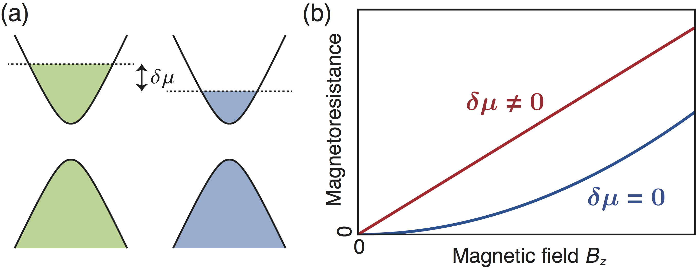
Figure 1: (a) Schematic illustration of valley polarization due to
a chemical potential difference δ μ 𝛿 𝜇 \delta\mu B z subscript 𝐵 𝑧 B_{z} δ μ ≠ 0 𝛿 𝜇 0 \delta\mu\neq 0 B z subscript 𝐵 𝑧 B_{z} δ μ = 0 𝛿 𝜇 0 \delta\mu=0
Magnetotransport theory.—
The transport theory
we employ is valid in the low magnetic field regime where Landau quantization
can be neglected and enables us to systematically compute the conductivity tensor in the presence of
disorder in arbitrary spatial dimensions. It is based on a quantum kinetic equation that accounts for
disorder, and for electric 𝑬 𝑬 \bm{E} 𝑩 𝑩 \bm{B} Sekine2017 ; Comment6
∂ ⟨ ρ ⟩ ∂ t + i ℏ [ ℋ 0 , ⟨ ρ ⟩ ] + K ( ⟨ ρ ⟩ ) = D E ( ⟨ ρ ⟩ ) + D B ( ⟨ ρ ⟩ ) , delimited-⟨⟩ 𝜌 𝑡 𝑖 Planck-constant-over-2-pi subscript ℋ 0 delimited-⟨⟩ 𝜌 𝐾 delimited-⟨⟩ 𝜌 subscript 𝐷 𝐸 delimited-⟨⟩ 𝜌 subscript 𝐷 𝐵 delimited-⟨⟩ 𝜌 \displaystyle\frac{\partial\langle\rho\rangle}{\partial t}+\frac{i}{\hbar}[\mathcal{H}_{0},\langle\rho\rangle]+K(\langle\rho\rangle)=D_{E}(\langle\rho\rangle)+D_{B}(\langle\rho\rangle), (1)
where ⟨ ρ ⟩ delimited-⟨⟩ 𝜌 \langle\rho\rangle ℋ 0 subscript ℋ 0 \mathcal{H}_{0} K ( ⟨ ρ ⟩ ) 𝐾 delimited-⟨⟩ 𝜌 K(\langle\rho\rangle) D E ( ⟨ ρ ⟩ ) subscript 𝐷 𝐸 delimited-⟨⟩ 𝜌 D_{E}(\langle\rho\rangle) D B ( ⟨ ρ ⟩ ) subscript 𝐷 𝐵 delimited-⟨⟩ 𝜌 D_{B}(\langle\rho\rangle)
D E ( ⟨ ρ ⟩ ) subscript 𝐷 𝐸 delimited-⟨⟩ 𝜌 \displaystyle D_{E}(\langle\rho\rangle) = e 𝑬 ℏ ⋅ D ⟨ ρ ⟩ D 𝒌 , absent ⋅ 𝑒 𝑬 Planck-constant-over-2-pi 𝐷 delimited-⟨⟩ 𝜌 𝐷 𝒌 \displaystyle=\frac{e\bm{E}}{\hbar}\cdot\frac{D\langle\rho\rangle}{D\bm{k}},
D B ( ⟨ ρ ⟩ ) subscript 𝐷 𝐵 delimited-⟨⟩ 𝜌 \displaystyle D_{B}(\langle\rho\rangle) = e 2 ℏ 2 { ( D ℋ 0 D 𝒌 × 𝑩 ) ⋅ D ⟨ ρ ⟩ D 𝒌 } . absent 𝑒 2 superscript Planck-constant-over-2-pi 2 ⋅ 𝐷 subscript ℋ 0 𝐷 𝒌 𝑩 𝐷 delimited-⟨⟩ 𝜌 𝐷 𝒌 \displaystyle=\frac{e}{2\hbar^{2}}\left\{\left(\frac{D\mathcal{H}_{0}}{D\bm{k}}\times\bm{B}\right)\cdot\frac{D\langle\rho\rangle}{D\bm{k}}\right\}. (2)
Here, e > 0 𝑒 0 e>0 𝒌 𝒌 \bm{k} { 𝒂 ⋅ 𝒃 } = 𝒂 ⋅ 𝒃 + 𝒃 ⋅ 𝒂 ⋅ 𝒂 𝒃 ⋅ 𝒂 𝒃 ⋅ 𝒃 𝒂 \{\bm{a}\cdot\bm{b}\}=\bm{a}\cdot\bm{b}+\bm{b}\cdot\bm{a} 𝒂 𝒂 \bm{a} 𝒃 𝒃 \bm{b} X 𝑋 X = ⟨ ρ ⟩ , ℋ 0 absent delimited-⟨⟩ 𝜌 subscript ℋ 0
=\langle\rho\rangle,\mathcal{H}_{0}
D X D 𝒌 = ∂ X ∂ 𝒌 − i [ 𝓡 𝒌 , X ] , 𝐷 𝑋 𝐷 𝒌 𝑋 𝒌 𝑖 subscript 𝓡 𝒌 𝑋 \displaystyle\frac{DX}{D\bm{k}}=\frac{\partial X}{\partial\bm{k}}-i[\bm{\mathcal{R}}_{\bm{k}},X], (3)
where 𝓡 𝒌 = ∑ α = x , y , z ℛ 𝒌 , α 𝒆 α subscript 𝓡 𝒌 subscript 𝛼 𝑥 𝑦 𝑧
subscript ℛ 𝒌 𝛼
subscript 𝒆 𝛼 \bm{\mathcal{R}}_{\bm{k}}=\sum_{\alpha=x,y,z}\mathcal{R}_{\bm{k},\alpha}\bm{e}_{\alpha} [ ℛ 𝒌 , α ] m n = i ⟨ u 𝒌 m | ∂ k α u 𝒌 n ⟩ superscript delimited-[] subscript ℛ 𝒌 𝛼
𝑚 𝑛 𝑖 inner-product subscript superscript 𝑢 𝑚 𝒌 subscript subscript 𝑘 𝛼 subscript superscript 𝑢 𝑛 𝒌 [\mathcal{R}_{\bm{k},\alpha}]^{mn}=i\langle u^{m}_{\bm{k}}|\partial_{k_{\alpha}}u^{n}_{\bm{k}}\rangle
The steady-state linear response of the density matrix to an electric field can be expressed as
a formal expansion in powers of the magnetic field strength B 𝐵 B Sekine2017 ; Comment5 ⟨ ρ ⟩ = ( 1 − ℒ − 1 D B ) − 1 ℒ − 1 D E ( ⟨ ρ 0 ⟩ + ⟨ Ξ B ⟩ ) ≡ ⟨ ρ E ⟩ + ∑ N ≥ 1 ⟨ ρ B , N ⟩ delimited-⟨⟩ 𝜌 superscript 1 superscript ℒ 1 subscript 𝐷 𝐵 1 superscript ℒ 1 subscript 𝐷 𝐸 delimited-⟨⟩ subscript 𝜌 0 delimited-⟨⟩ subscript Ξ 𝐵 delimited-⟨⟩ subscript 𝜌 𝐸 subscript 𝑁 1 delimited-⟨⟩ subscript 𝜌 𝐵 𝑁
\langle\rho\rangle=(1-\mathcal{L}^{-1}D_{B})^{-1}\mathcal{L}^{-1}D_{E}(\langle\rho_{0}\rangle+\langle\Xi_{B}\rangle)\equiv\langle\rho_{E}\rangle+\sum_{N\geq 1}\langle\rho_{B,N}\rangle ⟨ ρ E ⟩ = ℒ − 1 D E ( ⟨ ρ 0 ⟩ ) delimited-⟨⟩ subscript 𝜌 𝐸 superscript ℒ 1 subscript 𝐷 𝐸 delimited-⟨⟩ subscript 𝜌 0 \langle\rho_{E}\rangle=\mathcal{L}^{-1}D_{E}(\langle\rho_{0}\rangle) ⟨ ρ B , N ⟩ = ( ℒ − 1 D B ) N ℒ − 1 D E ( ⟨ ρ 0 ⟩ ) + ( ℒ − 1 D B ) N − 1 ℒ − 1 D E ( ⟨ Ξ B ⟩ ) delimited-⟨⟩ subscript 𝜌 𝐵 𝑁
superscript superscript ℒ 1 subscript 𝐷 𝐵 𝑁 superscript ℒ 1 subscript 𝐷 𝐸 delimited-⟨⟩ subscript 𝜌 0 superscript superscript ℒ 1 subscript 𝐷 𝐵 𝑁 1 superscript ℒ 1 subscript 𝐷 𝐸 delimited-⟨⟩ subscript Ξ 𝐵 \langle\rho_{B,N}\rangle=(\mathcal{L}^{-1}D_{B})^{N}\mathcal{L}^{-1}D_{E}(\langle\rho_{0}\rangle)+(\mathcal{L}^{-1}D_{B})^{N-1}\mathcal{L}^{-1}D_{E}(\langle\Xi_{B}\rangle) ℒ ≡ P + K ℒ 𝑃 𝐾 \mathcal{L}\equiv P+K P ⟨ ρ ⟩ ≡ ( i / ℏ ) [ ℋ 0 , ⟨ ρ ⟩ ] 𝑃 delimited-⟨⟩ 𝜌 𝑖 Planck-constant-over-2-pi subscript ℋ 0 delimited-⟨⟩ 𝜌 P\langle\rho\rangle\equiv(i/\hbar)\,[\mathcal{H}_{0},\langle\rho\rangle] ⟨ ρ 0 ⟩ delimited-⟨⟩ subscript 𝜌 0 \langle\rho_{0}\rangle ⟨ Ξ B ⟩ delimited-⟨⟩ subscript Ξ 𝐵 \langle\Xi_{B}\rangle ⟨ Ξ B ⟩ delimited-⟨⟩ subscript Ξ 𝐵 \langle\Xi_{B}\rangle Xiao2005
Throughout this Rapid Communication, we work in the eigenstate basis for the various contributions to the
steady-state density matrix, and decompose
⟨ ρ B , N ⟩ delimited-⟨⟩ subscript 𝜌 𝐵 𝑁
\langle\rho_{B,N}\rangle ⟨ n B , N ⟩ + ⟨ ξ B , N ⟩ delimited-⟨⟩ subscript 𝑛 𝐵 𝑁
delimited-⟨⟩ subscript 𝜉 𝐵 𝑁
\langle n_{B,N}\rangle+\langle\xi_{B,N}\rangle ⟨ S B , N ⟩ delimited-⟨⟩ subscript 𝑆 𝐵 𝑁
\langle S_{B,N}\rangle ⟨ ρ B , N ⟩ delimited-⟨⟩ subscript 𝜌 𝐵 𝑁
\langle\rho_{B,N}\rangle
⟨ n B , N ⟩ 𝒌 m m superscript subscript delimited-⟨⟩ subscript 𝑛 𝐵 𝑁
𝒌 𝑚 𝑚 \displaystyle\langle n_{B,N}\rangle_{\bm{k}}^{mm} = τ m [ D B ( ⟨ ρ B , N − 1 ⟩ ) ] 𝒌 m m , absent subscript 𝜏 𝑚 superscript subscript delimited-[] subscript 𝐷 𝐵 delimited-⟨⟩ subscript 𝜌 𝐵 𝑁 1
𝒌 𝑚 𝑚 \displaystyle=\tau_{m}[D_{B}(\langle\rho_{B,N-1}\rangle)]_{\bm{k}}^{mm},
⟨ ξ B , N ⟩ 𝒌 m m superscript subscript delimited-⟨⟩ subscript 𝜉 𝐵 𝑁
𝒌 𝑚 𝑚 \displaystyle\langle\xi_{B,N}\rangle_{\bm{k}}^{mm} = e ℏ 𝑩 ⋅ 𝛀 𝒌 m ⟨ n B , N − 1 ⟩ 𝒌 m m , absent ⋅ 𝑒 Planck-constant-over-2-pi 𝑩 superscript subscript 𝛀 𝒌 𝑚 superscript subscript delimited-⟨⟩ subscript 𝑛 𝐵 𝑁 1
𝒌 𝑚 𝑚 \displaystyle=\frac{e}{\hbar}\bm{B}\cdot\bm{\Omega}_{\bm{k}}^{m}\,\langle n_{B,N-1}\rangle_{\bm{k}}^{mm}, (4)
where N ≥ 1 𝑁 1 N\geq 1 ⟨ ρ B , 0 ⟩ = ⟨ ρ E ⟩ delimited-⟨⟩ subscript 𝜌 𝐵 0
delimited-⟨⟩ subscript 𝜌 𝐸 \langle\rho_{B,0}\rangle=\langle\rho_{E}\rangle ⟨ n B , 0 ⟩ = 2 ⟨ n E ⟩ delimited-⟨⟩ subscript 𝑛 𝐵 0
2 delimited-⟨⟩ subscript 𝑛 𝐸 \langle n_{B,0}\rangle=2\langle n_{E}\rangle τ m subscript 𝜏 𝑚 \tau_{m} 𝛀 𝒌 m superscript subscript 𝛀 𝒌 𝑚 \bm{\Omega}_{\bm{k}}^{m} m 𝑚 m ⟨ Ξ B ⟩ 𝒌 m m = ( e / ℏ ) 𝑩 ⋅ 𝛀 𝒌 m ⟨ ρ 0 ⟩ 𝒌 m m subscript superscript delimited-⟨⟩ subscript Ξ 𝐵 𝑚 𝑚 𝒌 ⋅ 𝑒 Planck-constant-over-2-pi 𝑩 superscript subscript 𝛀 𝒌 𝑚 subscript superscript delimited-⟨⟩ subscript 𝜌 0 𝑚 𝑚 𝒌 \langle\Xi_{B}\rangle^{mm}_{\bm{k}}=(e/\hbar)\bm{B}\cdot\bm{\Omega}_{\bm{k}}^{m}\langle\rho_{0}\rangle^{mm}_{\bm{k}} 4 ⟨ n B , N ⟩ delimited-⟨⟩ subscript 𝑛 𝐵 𝑁
\langle n_{B,N}\rangle ⟨ ξ B , N ⟩ delimited-⟨⟩ subscript 𝜉 𝐵 𝑁
\langle\xi_{B,N}\rangle Sekine2017
⟨ S B , N ⟩ 𝒌 m m ′ = ℏ i [ D B ( ⟨ ρ B , N − 1 ⟩ ) ] 𝒌 m m ′ − [ J ( ⟨ n B , N ⟩ ) ] 𝒌 m m ′ ε 𝒌 m − ε 𝒌 m ′ , superscript subscript delimited-⟨⟩ subscript 𝑆 𝐵 𝑁
𝒌 𝑚 superscript 𝑚 ′ Planck-constant-over-2-pi 𝑖 superscript subscript delimited-[] subscript 𝐷 𝐵 delimited-⟨⟩ subscript 𝜌 𝐵 𝑁 1
𝒌 𝑚 superscript 𝑚 ′ superscript subscript delimited-[] 𝐽 delimited-⟨⟩ subscript 𝑛 𝐵 𝑁
𝒌 𝑚 superscript 𝑚 ′ superscript subscript 𝜀 𝒌 𝑚 superscript subscript 𝜀 𝒌 superscript 𝑚 ′ \displaystyle\langle S_{B,N}\rangle_{\bm{k}}^{mm^{\prime}}=\frac{\hbar}{i}\frac{[D_{B}(\langle\rho_{B,N-1}\rangle)]_{\bm{k}}^{mm^{\prime}}-[J(\langle n_{B,N}\rangle)]_{\bm{k}}^{mm^{\prime}}}{\varepsilon_{\bm{k}}^{m}-\varepsilon_{\bm{k}}^{m^{\prime}}}, (5)
where m ≠ m ′ 𝑚 superscript 𝑚 ′ m\neq m^{\prime} ε 𝒌 m superscript subscript 𝜀 𝒌 𝑚 \varepsilon_{\bm{k}}^{m} m 𝑚 m 5 D B ( ⟨ ρ B , N − 1 ⟩ ) subscript 𝐷 𝐵 delimited-⟨⟩ subscript 𝜌 𝐵 𝑁 1
D_{B}(\langle\rho_{B,N-1}\rangle) J ( ⟨ n B , N ⟩ ) 𝐽 delimited-⟨⟩ subscript 𝑛 𝐵 𝑁
J(\langle n_{B,N}\rangle) Culcer2017 ; Sekine2017 J ( ⟨ n B , N ⟩ ) 𝐽 delimited-⟨⟩ subscript 𝑛 𝐵 𝑁
J(\langle n_{B,N}\rangle)
Massive Dirac model.—
We consider 2D semiconductors with broken inversion symmetry, like monolayer TMDs,
that have two low-energy valleys related by time-reversal.
The low-energy effective Hamiltonians in these
systems normally have the massive Dirac form Xiao2007 ; Liu2011 ; Xiao2012
ℋ τ z ( 𝒌 ) = v F ( τ z k x σ x + k y σ y ) + m σ z . subscript ℋ subscript 𝜏 𝑧 𝒌 subscript 𝑣 𝐹 subscript 𝜏 𝑧 subscript 𝑘 𝑥 subscript 𝜎 𝑥 subscript 𝑘 𝑦 subscript 𝜎 𝑦 𝑚 subscript 𝜎 𝑧 \displaystyle\mathcal{H}_{\tau_{z}}(\bm{k})=v_{F}(\tau_{z}k_{x}\sigma_{x}+k_{y}\sigma_{y})+m\sigma_{z}. (6)
(As we discuss briefly later, gated bilayer graphene is an exception.)
In Eq. (6 τ z = ± 1 subscript 𝜏 𝑧 plus-or-minus 1 \tau_{z}=\pm 1 v F subscript 𝑣 𝐹 v_{F} 2 m 2 𝑚 2m σ i subscript 𝜎 𝑖 \sigma_{i} 6 ± ε 𝒌 = ± v F 2 ( k x 2 + k y 2 ) + m 2 plus-or-minus subscript 𝜀 𝒌 plus-or-minus superscript subscript 𝑣 𝐹 2 superscript subscript 𝑘 𝑥 2 superscript subscript 𝑘 𝑦 2 superscript 𝑚 2 \pm\varepsilon_{\bm{k}}=\pm\sqrt{v_{F}^{2}(k_{x}^{2}+k_{y}^{2})+m^{2}} | u 𝒌 ± ( τ z ) ⟩ ket superscript subscript 𝑢 𝒌 plus-or-minus subscript 𝜏 𝑧 |u_{\bm{k}}^{\pm}(\tau_{z})\rangle 3 | u 𝒌 ± ( τ z ) ⟩ ket superscript subscript 𝑢 𝒌 plus-or-minus subscript 𝜏 𝑧 |u_{\bm{k}}^{\pm}(\tau_{z})\rangle [ ℛ 𝒌 , α τ z ] m n = i ⟨ u 𝒌 m ( τ z ) | ∂ k α u 𝒌 n ( τ z ) ⟩ superscript delimited-[] subscript superscript ℛ subscript 𝜏 𝑧 𝒌 𝛼
𝑚 𝑛 𝑖 inner-product subscript superscript 𝑢 𝑚 𝒌 subscript 𝜏 𝑧 subscript subscript 𝑘 𝛼 subscript superscript 𝑢 𝑛 𝒌 subscript 𝜏 𝑧 [\mathcal{R}^{\tau_{z}}_{\bm{k},\alpha}]^{mn}=i\langle u^{m}_{\bm{k}}(\tau_{z})|\partial_{k_{\alpha}}u^{n}_{\bm{k}}(\tau_{z})\rangle m , n = ± 𝑚 𝑛
plus-or-minus m,n=\pm
ℛ 𝒌 , x τ z = subscript superscript ℛ subscript 𝜏 𝑧 𝒌 𝑥
absent \displaystyle\mathcal{R}^{\tau_{z}}_{\bm{k},x}=\, 1 2 k τ z sin θ − σ ~ z m 2 k ε 𝒌 τ z sin θ − σ ~ y v F m 2 ε 𝒌 2 cos θ 1 2 𝑘 subscript 𝜏 𝑧 𝜃 subscript ~ 𝜎 𝑧 𝑚 2 𝑘 subscript 𝜀 𝒌 subscript 𝜏 𝑧 𝜃 subscript ~ 𝜎 𝑦 subscript 𝑣 𝐹 𝑚 2 superscript subscript 𝜀 𝒌 2 𝜃 \displaystyle\frac{1}{2k}\tau_{z}\sin\theta-\tilde{\sigma}_{z}\frac{m}{2k\varepsilon_{\bm{k}}}\tau_{z}\sin\theta-\tilde{\sigma}_{y}\frac{v_{F}m}{2\varepsilon_{\bm{k}}^{2}}\cos\theta
− σ ~ x v F 2 ε 𝒌 τ z sin θ , subscript ~ 𝜎 𝑥 subscript 𝑣 𝐹 2 subscript 𝜀 𝒌 subscript 𝜏 𝑧 𝜃 \displaystyle-\tilde{\sigma}_{x}\frac{v_{F}}{2\varepsilon_{\bm{k}}}\tau_{z}\sin\theta,
ℛ 𝒌 , y τ z = subscript superscript ℛ subscript 𝜏 𝑧 𝒌 𝑦
absent \displaystyle\mathcal{R}^{\tau_{z}}_{\bm{k},y}=\, − 1 2 k τ z cos θ + σ ~ z m 2 k ε 𝒌 τ z cos θ − σ ~ y v F m 2 ε 𝒌 2 sin θ 1 2 𝑘 subscript 𝜏 𝑧 𝜃 subscript ~ 𝜎 𝑧 𝑚 2 𝑘 subscript 𝜀 𝒌 subscript 𝜏 𝑧 𝜃 subscript ~ 𝜎 𝑦 subscript 𝑣 𝐹 𝑚 2 superscript subscript 𝜀 𝒌 2 𝜃 \displaystyle-\frac{1}{2k}\tau_{z}\cos\theta+\tilde{\sigma}_{z}\frac{m}{2k\varepsilon_{\bm{k}}}\tau_{z}\cos\theta-\tilde{\sigma}_{y}\frac{v_{F}m}{2\varepsilon_{\bm{k}}^{2}}\sin\theta
+ σ ~ x v F 2 ε 𝒌 τ z cos θ , subscript ~ 𝜎 𝑥 subscript 𝑣 𝐹 2 subscript 𝜀 𝒌 subscript 𝜏 𝑧 𝜃 \displaystyle+\tilde{\sigma}_{x}\frac{v_{F}}{2\varepsilon_{\bm{k}}}\tau_{z}\cos\theta, (7)
where e ± i θ = ( k x ± i k y ) / k superscript 𝑒 plus-or-minus 𝑖 𝜃 plus-or-minus subscript 𝑘 𝑥 𝑖 subscript 𝑘 𝑦 𝑘 e^{\pm i\theta}=(k_{x}\pm ik_{y})/k k = k x 2 + k y 2 𝑘 superscript subscript 𝑘 𝑥 2 superscript subscript 𝑘 𝑦 2 k=\sqrt{k_{x}^{2}+k_{y}^{2}} σ ~ α subscript ~ 𝜎 𝛼 \tilde{\sigma}_{\alpha} [ Ω 𝒌 , z τ z ] ± = i ⟨ ∂ k x u 𝒌 ± ( τ z ) | ∂ k y u 𝒌 ± ( τ z ) ⟩ − i ⟨ ∂ k y u 𝒌 ± ( τ z ) | ∂ k x u 𝒌 ± ( τ z ) ⟩ = ∓ τ z v F 2 m / ( 2 ε 𝒌 3 ) superscript delimited-[] subscript superscript Ω subscript 𝜏 𝑧 𝒌 𝑧
plus-or-minus 𝑖 inner-product subscript subscript 𝑘 𝑥 superscript subscript 𝑢 𝒌 plus-or-minus subscript 𝜏 𝑧 subscript subscript 𝑘 𝑦 superscript subscript 𝑢 𝒌 plus-or-minus subscript 𝜏 𝑧 𝑖 inner-product subscript subscript 𝑘 𝑦 superscript subscript 𝑢 𝒌 plus-or-minus subscript 𝜏 𝑧 subscript subscript 𝑘 𝑥 superscript subscript 𝑢 𝒌 plus-or-minus subscript 𝜏 𝑧 minus-or-plus subscript 𝜏 𝑧 superscript subscript 𝑣 𝐹 2 𝑚 2 superscript subscript 𝜀 𝒌 3 [\Omega^{\tau_{z}}_{\bm{k},z}]^{\pm}=i\langle\partial_{k_{x}}u_{\bm{k}}^{\pm}(\tau_{z})|\partial_{k_{y}}u_{\bm{k}}^{\pm}(\tau_{z})\rangle-i\langle\partial_{k_{y}}u_{\bm{k}}^{\pm}(\tau_{z})|\partial_{k_{x}}u_{\bm{k}}^{\pm}(\tau_{z})\rangle=\mp\tau_{z}v_{F}^{2}m/(2\varepsilon_{\bm{k}}^{3})
Valley-dependent longitudinal magnetoconductivity.—
We apply our magnetotransport theory to the 2D systems described by Eq. (6 𝑩 = ( 0 , 0 , B z ) 𝑩 0 0 subscript 𝐵 𝑧 \bm{B}=(0,0,B_{z}) J 𝐽 J 5 μ 𝜇 \mu x x 𝑥 𝑥 xx
σ μ ν ( N ) ( B z ) = Tr [ ( − e ) v μ ⟨ ρ B , N ⟩ ] / E ν . subscript superscript 𝜎 𝑁 𝜇 𝜈 subscript 𝐵 𝑧 Tr delimited-[] 𝑒 subscript 𝑣 𝜇 delimited-⟨⟩ subscript 𝜌 𝐵 𝑁
subscript 𝐸 𝜈 \displaystyle\sigma^{(N)}_{\mu\nu}(B_{z})=\mathrm{Tr}\left[(-e)v_{\mu}\langle\rho_{B,N}\rangle\right]/E_{\nu}. (8)
In the eigenstate basis the velocity operator reads
v x = v F ( σ ~ z v F k ε 𝒌 cos θ + σ ~ y τ z sin θ − σ ~ x m ε 𝒌 cos θ ) subscript 𝑣 𝑥 subscript 𝑣 𝐹 subscript ~ 𝜎 𝑧 subscript 𝑣 𝐹 𝑘 subscript 𝜀 𝒌 𝜃 subscript ~ 𝜎 𝑦 subscript 𝜏 𝑧 𝜃 subscript ~ 𝜎 𝑥 𝑚 subscript 𝜀 𝒌 𝜃 v_{x}=v_{F}(\tilde{\sigma}_{z}\frac{v_{F}k}{\varepsilon_{\bm{k}}}\cos\theta+\tilde{\sigma}_{y}\tau_{z}\sin\theta-\tilde{\sigma}_{x}\frac{m}{\varepsilon_{\bm{k}}}\cos\theta)
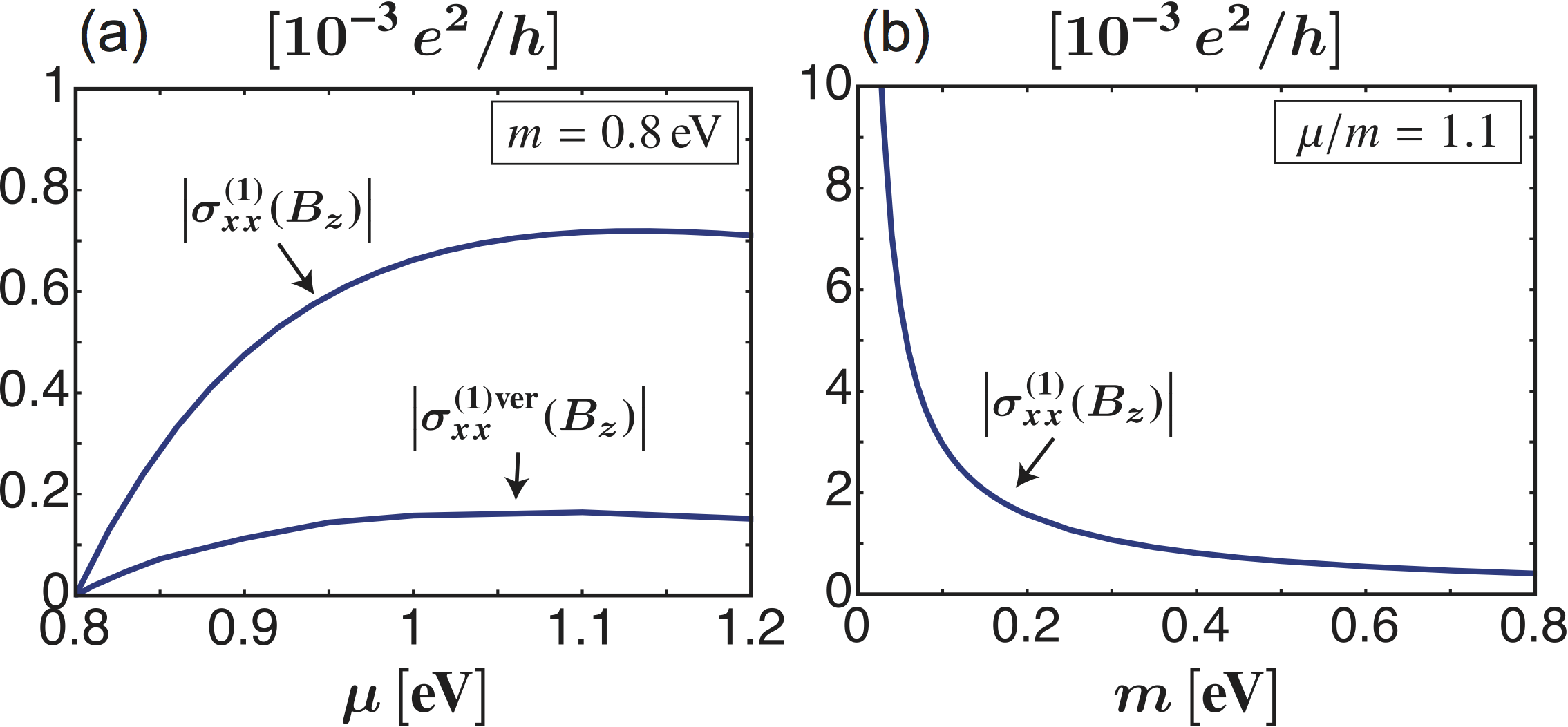
We first evaluate the magnetoconductivity contributions proportional to odd powers of B z subscript 𝐵 𝑧 B_{z} μ > m 𝜇 𝑚 \mu>m σ x x ( 1 ) ( B z ) superscript subscript 𝜎 𝑥 𝑥 1 subscript 𝐵 𝑧 \sigma_{xx}^{(1)}(B_{z}) ⟨ ρ B , 1 ⟩ = ℒ − 1 D B ( ⟨ ρ E ⟩ ) + ℒ − 1 D E ( ⟨ Ξ B ⟩ ) delimited-⟨⟩ subscript 𝜌 𝐵 1
superscript ℒ 1 subscript 𝐷 𝐵 delimited-⟨⟩ subscript 𝜌 𝐸 superscript ℒ 1 subscript 𝐷 𝐸 delimited-⟨⟩ subscript Ξ 𝐵 \langle\rho_{B,1}\rangle=\mathcal{L}^{-1}D_{B}(\langle\rho_{E}\rangle)+\mathcal{L}^{-1}D_{E}(\langle\Xi_{B}\rangle) Comment1
σ x x ( 1 ) ( B z ) superscript subscript 𝜎 𝑥 𝑥 1 subscript 𝐵 𝑧 \displaystyle\sigma_{xx}^{(1)}(B_{z}) = τ z e 2 B z E x ∫ [ d 𝒌 ] [ v F 2 m 2 ε 𝒌 2 ∂ ∂ k x + v F 4 m k x ε 𝒌 4 ] ⟨ n E ⟩ 𝒌 + + absent subscript 𝜏 𝑧 superscript 𝑒 2 subscript 𝐵 𝑧 subscript 𝐸 𝑥 delimited-[] 𝑑 𝒌 delimited-[] superscript subscript 𝑣 𝐹 2 𝑚 2 superscript subscript 𝜀 𝒌 2 subscript 𝑘 𝑥 superscript subscript 𝑣 𝐹 4 𝑚 subscript 𝑘 𝑥 superscript subscript 𝜀 𝒌 4 superscript subscript delimited-⟨⟩ subscript 𝑛 𝐸 𝒌 absent \displaystyle=\tau_{z}\frac{e^{2}B_{z}}{E_{x}}\int[d\bm{k}]\left[\frac{v_{F}^{2}m}{2\varepsilon_{\bm{k}}^{2}}\frac{\partial}{\partial k_{x}}+\frac{v_{F}^{4}mk_{x}}{\varepsilon_{\bm{k}}^{4}}\right]\langle n_{E}\rangle_{\bm{k}}^{++}
≡ τ z e 3 ℏ B z v F 2 𝒞 1 ( μ , m ) τ tr , absent subscript 𝜏 𝑧 superscript 𝑒 3 Planck-constant-over-2-pi subscript 𝐵 𝑧 superscript subscript 𝑣 𝐹 2 subscript 𝒞 1 𝜇 𝑚 subscript 𝜏 tr \displaystyle\equiv\tau_{z}\frac{e^{3}}{\hbar}B_{z}v_{F}^{2}\mathcal{C}_{1}(\mu,m)\tau_{\mathrm{tr}}, (9)
where [ d 𝒌 ] ≡ d 2 k ( 2 π ) 2 delimited-[] 𝑑 𝒌 superscript 𝑑 2 𝑘 superscript 2 𝜋 2 [d\bm{k}]\equiv\frac{d^{2}k}{(2\pi)^{2}} ⟨ n E ⟩ 𝒌 + + = τ tr ( e E x / ℏ ) ∂ f 0 ( ε 𝒌 ) / ∂ k x superscript subscript delimited-⟨⟩ subscript 𝑛 𝐸 𝒌 absent subscript 𝜏 tr 𝑒 subscript 𝐸 𝑥 Planck-constant-over-2-pi subscript 𝑓 0 subscript 𝜀 𝒌 subscript 𝑘 𝑥 \langle n_{E}\rangle_{\bm{k}}^{++}=\tau_{\mathrm{tr}}(eE_{x}/\hbar)\partial f_{0}(\varepsilon_{\bm{k}})/\partial k_{x} f 0 ( ε 𝒌 ) subscript 𝑓 0 subscript 𝜀 𝒌 f_{0}(\varepsilon_{\bm{k}}) τ tr subscript 𝜏 tr \tau_{\mathrm{tr}} 𝒞 1 ( μ , m ) < 0 subscript 𝒞 1 𝜇 𝑚 0 \mathcal{C}_{1}(\mu,m)<0 9 ⟨ n E ⟩ delimited-⟨⟩ subscript 𝑛 𝐸 \langle n_{E}\rangle ⟨ S B , 1 ⟩ delimited-⟨⟩ subscript 𝑆 𝐵 1
\langle S_{B,1}\rangle ⟨ ξ B , 1 ⟩ delimited-⟨⟩ subscript 𝜉 𝐵 1
\langle\xi_{B,1}\rangle 2 μ 𝜇 \mu m 𝑚 m σ x x ( 1 ) ( B z ) superscript subscript 𝜎 𝑥 𝑥 1 subscript 𝐵 𝑧 \sigma_{xx}^{(1)}(B_{z}) 2 σ x x ( 1 ) ( B z ) superscript subscript 𝜎 𝑥 𝑥 1 subscript 𝐵 𝑧 \sigma_{xx}^{(1)}(B_{z})
Figure 2:
(a) Chemical potential μ 𝜇 \mu σ x x ( 1 ) ( B z ) superscript subscript 𝜎 𝑥 𝑥 1 subscript 𝐵 𝑧 \sigma_{xx}^{(1)}(B_{z}) 9 σ x x ( 1 ) ver ( B z ) superscript subscript 𝜎 𝑥 𝑥 1 ver subscript 𝐵 𝑧 \sigma_{xx}^{(1)\mathrm{ver}}(B_{z}) 14 m = 0.8 eV 𝑚 0.8 eV m=0.8\,\mathrm{eV} σ x x ( 1 ) ( B z ) superscript subscript 𝜎 𝑥 𝑥 1 subscript 𝐵 𝑧 \sigma_{xx}^{(1)}(B_{z}) σ x x ( 1 ) ver ( B z ) superscript subscript 𝜎 𝑥 𝑥 1 ver subscript 𝐵 𝑧 \sigma_{xx}^{(1)\mathrm{ver}}(B_{z}) m / μ 2 𝑚 superscript 𝜇 2 m/\mu^{2} μ ≫ m much-greater-than 𝜇 𝑚 \mu\gg m μ ≫ m much-greater-than 𝜇 𝑚 \mu\gg m m 𝑚 m σ x x ( 1 ) ( B z ) superscript subscript 𝜎 𝑥 𝑥 1 subscript 𝐵 𝑧 \sigma_{xx}^{(1)}(B_{z}) μ / m = 1.1 𝜇 𝑚 1.1 \mu/m=1.1 B z = 0.1 T subscript 𝐵 𝑧 0.1 T B_{z}=0.1\,\mathrm{T} v F = 3 eV ⋅ Å subscript 𝑣 𝐹 ⋅ 3 eV Å v_{F}=3\,\mathrm{eV\cdot\AA} τ tr = 0.1 ps subscript 𝜏 tr 0.1 ps \tau_{\mathrm{tr}}=0.1\,\mathrm{ps} T = 5 meV 𝑇 5 meV T=5\,\mathrm{meV}
Similarly, we find the cubic magnetoconductivity obtained from ⟨ ρ B , 3 ⟩ delimited-⟨⟩ subscript 𝜌 𝐵 3
\langle\rho_{B,3}\rangle Comment1
σ x x ( 3 ) ( B z ) subscript superscript 𝜎 3 𝑥 𝑥 subscript 𝐵 𝑧 \displaystyle\sigma^{(3)}_{xx}(B_{z}) = 8 3 τ z e 2 B z E x ∫ [ d 𝒌 ] [ v F 2 m 2 ε 𝒌 2 ∂ ∂ k x + v F 4 m k x 2 ε 𝒌 4 ] ⟨ n B , 2 ⟩ 𝒌 + + absent 8 3 subscript 𝜏 𝑧 superscript 𝑒 2 subscript 𝐵 𝑧 subscript 𝐸 𝑥 delimited-[] 𝑑 𝒌 delimited-[] superscript subscript 𝑣 𝐹 2 𝑚 2 superscript subscript 𝜀 𝒌 2 subscript 𝑘 𝑥 superscript subscript 𝑣 𝐹 4 𝑚 subscript 𝑘 𝑥 2 superscript subscript 𝜀 𝒌 4 superscript subscript delimited-⟨⟩ subscript 𝑛 𝐵 2
𝒌 absent \displaystyle=\frac{8}{3}\tau_{z}\frac{e^{2}B_{z}}{E_{x}}\int[d\bm{k}]\left[\frac{v_{F}^{2}m}{2\varepsilon_{\bm{k}}^{2}}\frac{\partial}{\partial k_{x}}+\frac{v_{F}^{4}mk_{x}}{2\varepsilon_{\bm{k}}^{4}}\right]\langle n_{B,2}\rangle_{\bm{k}}^{++}
≡ τ z e 5 ℏ B z 3 v F 6 𝒞 3 ( μ , m ) τ tr 3 , absent subscript 𝜏 𝑧 superscript 𝑒 5 Planck-constant-over-2-pi superscript subscript 𝐵 𝑧 3 superscript subscript 𝑣 𝐹 6 subscript 𝒞 3 𝜇 𝑚 superscript subscript 𝜏 tr 3 \displaystyle\equiv\tau_{z}\frac{e^{5}}{\hbar}B_{z}^{3}v_{F}^{6}\mathcal{C}_{3}(\mu,m)\tau_{\mathrm{tr}}^{3}, (10)
where ⟨ n B , 2 ⟩ 𝒌 + + = ( e B z τ tr ) 2 ( ∂ ε 𝒌 ∂ k y ∂ ∂ k x − ∂ ε 𝒌 ∂ k x ∂ ∂ k y ) 2 ⟨ n E ⟩ 𝒌 + + superscript subscript delimited-⟨⟩ subscript 𝑛 𝐵 2
𝒌 absent superscript 𝑒 subscript 𝐵 𝑧 subscript 𝜏 tr 2 superscript subscript 𝜀 𝒌 subscript 𝑘 𝑦 subscript 𝑘 𝑥 subscript 𝜀 𝒌 subscript 𝑘 𝑥 subscript 𝑘 𝑦 2 superscript subscript delimited-⟨⟩ subscript 𝑛 𝐸 𝒌 absent \langle n_{B,2}\rangle_{\bm{k}}^{++}=(eB_{z}\tau_{\mathrm{tr}})^{2}(\frac{\partial\varepsilon_{\bm{k}}}{\partial k_{y}}\frac{\partial}{\partial k_{x}}-\frac{\partial\varepsilon_{\bm{k}}}{\partial k_{x}}\frac{\partial}{\partial k_{y}})^{2}\langle n_{E}\rangle_{\bm{k}}^{++} 𝒞 3 ( μ , m ) > 0 subscript 𝒞 3 𝜇 𝑚 0 \mathcal{C}_{3}(\mu,m)>0 μ ≫ m much-greater-than 𝜇 𝑚 \mu\gg m 𝒞 3 ( μ , m ) ∝ m / μ 4 proportional-to subscript 𝒞 3 𝜇 𝑚 𝑚 superscript 𝜇 4 \mathcal{C}_{3}(\mu,m)\propto m/\mu^{4} 2 | σ x x ( 3 ) ( B z ) / σ x x ( 1 ) ( B z ) | ∼ 10 − 3 ( B z [ T ] ) 2 similar-to subscript superscript 𝜎 3 𝑥 𝑥 subscript 𝐵 𝑧 subscript superscript 𝜎 1 𝑥 𝑥 subscript 𝐵 𝑧 superscript 10 3 superscript subscript 𝐵 𝑧 delimited-[] T 2 |\sigma^{(3)}_{xx}(B_{z})/\sigma^{(1)}_{xx}(B_{z})|\sim 10^{-3}(B_{z}\,[\rm{T}])^{2} 10 ⟨ n B , 2 ⟩ delimited-⟨⟩ subscript 𝑛 𝐵 2
\langle n_{B,2}\rangle ⟨ S B , 3 ⟩ delimited-⟨⟩ subscript 𝑆 𝐵 3
\langle S_{B,3}\rangle ⟨ ξ B , 3 ⟩ delimited-⟨⟩ subscript 𝜉 𝐵 3
\langle\xi_{B,3}\rangle
σ x x ( N ) ( B z ) = τ z e N + 2 ℏ B z N v F 2 N 𝒞 N ( μ , m ) τ tr N , subscript superscript 𝜎 𝑁 𝑥 𝑥 subscript 𝐵 𝑧 subscript 𝜏 𝑧 superscript 𝑒 𝑁 2 Planck-constant-over-2-pi superscript subscript 𝐵 𝑧 𝑁 superscript subscript 𝑣 𝐹 2 𝑁 subscript 𝒞 𝑁 𝜇 𝑚 superscript subscript 𝜏 tr 𝑁 \displaystyle\sigma^{(N)}_{xx}(B_{z})=\tau_{z}\frac{e^{N+2}}{\hbar}B_{z}^{N}v_{F}^{2N}\mathcal{C}_{N}(\mu,m)\tau_{\mathrm{tr}}^{N}, (11)
where N = 5 , 7 , 9 ⋯ 𝑁 5 7 9 ⋯
N=5,7,9\cdots 𝒞 N ( μ , m ) subscript 𝒞 𝑁 𝜇 𝑚 \mathcal{C}_{N}(\mu,m) -N
Next, we consider the magnetoconductivity contributions proportional to even powers of B z subscript 𝐵 𝑧 B_{z} Comment2 ⟨ ρ B , 2 ⟩ delimited-⟨⟩ subscript 𝜌 𝐵 2
\langle\rho_{B,2}\rangle
σ x x ( 2 ) ( B z ) subscript superscript 𝜎 2 𝑥 𝑥 subscript 𝐵 𝑧 \displaystyle\sigma^{(2)}_{xx}(B_{z}) ≈ − e 3 B z 2 τ tr 2 E x ∫ [ d 𝒌 ] v F 2 k x ε 𝒌 ( ∂ ε 𝒌 ∂ k y ∂ ∂ k x − ∂ ε 𝒌 ∂ k x ∂ ∂ k y ) 2 ⟨ n E ⟩ 𝒌 + + absent superscript 𝑒 3 superscript subscript 𝐵 𝑧 2 superscript subscript 𝜏 tr 2 subscript 𝐸 𝑥 delimited-[] 𝑑 𝒌 superscript subscript 𝑣 𝐹 2 subscript 𝑘 𝑥 subscript 𝜀 𝒌 superscript subscript 𝜀 𝒌 subscript 𝑘 𝑦 subscript 𝑘 𝑥 subscript 𝜀 𝒌 subscript 𝑘 𝑥 subscript 𝑘 𝑦 2 superscript subscript delimited-⟨⟩ subscript 𝑛 𝐸 𝒌 absent \displaystyle\approx-\frac{e^{3}B_{z}^{2}\tau_{\mathrm{tr}}^{2}}{E_{x}}\int[d\bm{k}]\frac{v_{F}^{2}k_{x}}{\varepsilon_{\bm{k}}}\biggl{(}\frac{\partial\varepsilon_{\bm{k}}}{\partial k_{y}}\frac{\partial}{\partial k_{x}}-\frac{\partial\varepsilon_{\bm{k}}}{\partial k_{x}}\frac{\partial}{\partial k_{y}}\biggr{)}^{2}\langle n_{E}\rangle_{\bm{k}}^{++}
= − σ x x ( 0 ) ( ω c τ tr ) 2 , absent superscript subscript 𝜎 𝑥 𝑥 0 superscript subscript 𝜔 𝑐 subscript 𝜏 tr 2 \displaystyle=-\sigma_{xx}^{(0)}(\omega_{c}\tau_{\mathrm{tr}})^{2}, (12)
where σ x x ( 0 ) = ( − e / E x ) ∫ [ d 𝒌 ] ( v F 2 k x / ε 𝒌 ) ⟨ n E ⟩ 𝒌 + + superscript subscript 𝜎 𝑥 𝑥 0 𝑒 subscript 𝐸 𝑥 delimited-[] 𝑑 𝒌 superscript subscript 𝑣 𝐹 2 subscript 𝑘 𝑥 subscript 𝜀 𝒌 superscript subscript delimited-⟨⟩ subscript 𝑛 𝐸 𝒌 absent \sigma_{xx}^{(0)}=(-e/E_{x})\int[d\bm{k}](v_{F}^{2}k_{x}/\varepsilon_{\bm{k}})\langle n_{E}\rangle_{\bm{k}}^{++} ω c = e B z v F 2 / μ subscript 𝜔 𝑐 𝑒 subscript 𝐵 𝑧 superscript subscript 𝑣 𝐹 2 𝜇 \omega_{c}=eB_{z}v_{F}^{2}/\mu ∼ 1 / ( μ τ tr ) 2 ≪ 1 similar-to absent 1 superscript 𝜇 subscript 𝜏 tr 2 much-less-than 1 \sim 1/(\mu\tau_{\mathrm{tr}})^{2}\ll 1 S24 Comment1
Vertex corrections.—
From Eq. (5 B z subscript 𝐵 𝑧 B_{z} ⟨ S B , 1 ′ ⟩ 𝒌 m m ′′ ≡ i ℏ [ J ( ⟨ n B , 1 ⟩ ) ] 𝒌 m m ′′ / ( ε 𝒌 m − ε 𝒌 m ′′ ) subscript superscript delimited-⟨⟩ subscript superscript 𝑆 ′ 𝐵 1
𝑚 superscript 𝑚 ′′ 𝒌 𝑖 Planck-constant-over-2-pi subscript superscript delimited-[] 𝐽 delimited-⟨⟩ subscript 𝑛 𝐵 1
𝑚 superscript 𝑚 ′′ 𝒌 superscript subscript 𝜀 𝒌 𝑚 superscript subscript 𝜀 𝒌 superscript 𝑚 ′′ \langle S^{\prime}_{B,1}\rangle^{mm^{\prime\prime}}_{\bm{k}}\equiv i\hbar[J(\langle n_{B,1}\rangle)]^{mm^{\prime\prime}}_{\bm{k}}/(\varepsilon_{\bm{k}}^{m}-\varepsilon_{\bm{k}}^{m^{\prime\prime}}) Culcer2017
[ J ( ⟨ n ⟩ ) ] 𝒌 m m ′′ = subscript superscript delimited-[] 𝐽 delimited-⟨⟩ 𝑛 𝑚 superscript 𝑚 ′′ 𝒌 absent \displaystyle[J(\langle n\rangle)]^{mm^{\prime\prime}}_{\bm{k}}= π ℏ ∑ m ′ 𝒌 ′ ⟨ U 𝒌 𝒌 ′ m m ′ U 𝒌 ′ 𝒌 m ′ m ′′ ⟩ [ ( n 𝒌 m − n 𝒌 ′ m ′ ) δ ( ε 𝒌 m − ε 𝒌 ′ m ′ ) \displaystyle\ \frac{\pi}{\hbar}\sum_{m^{\prime}\bm{k}^{\prime}}\langle U^{mm^{\prime}}_{\bm{k}\bm{k}^{\prime}}U^{m^{\prime}m^{\prime\prime}}_{\bm{k}^{\prime}\bm{k}}\rangle\left[(n^{m}_{\bm{k}}-n^{m^{\prime}}_{\bm{k}^{\prime}})\delta(\varepsilon^{m}_{\bm{k}}-\varepsilon^{m^{\prime}}_{\bm{k}^{\prime}})\right.
+ ( n 𝒌 m ′′ − n 𝒌 ′ m ′ ) δ ( ε 𝒌 m ′′ − ε 𝒌 ′ m ′ ) ] . \displaystyle\left.+\,(n^{m^{\prime\prime}}_{\bm{k}}-n^{m^{\prime}}_{\bm{k}^{\prime}})\delta(\varepsilon^{m^{\prime\prime}}_{\bm{k}}-\varepsilon^{m^{\prime}}_{\bm{k}^{\prime}})\right]. (13)
Here, m ≠ m ′′ 𝑚 superscript 𝑚 ′′ m\neq m^{\prime\prime} ⟨ n ⟩ = diag [ n 𝒌 m ] delimited-⟨⟩ 𝑛 diag delimited-[] subscript superscript 𝑛 𝑚 𝒌 \langle n\rangle=\mathrm{diag}[n^{m}_{\bm{k}}] U ( 𝒓 ) = U 0 ∑ i δ ( 𝒓 − 𝒓 i ) 𝑈 𝒓 subscript 𝑈 0 subscript 𝑖 𝛿 𝒓 subscript 𝒓 𝑖 U(\bm{r})=U_{0}\sum_{i}\delta(\bm{r}-\bm{r}_{i}) ⟨ U ( 𝒓 ) U ( 𝒓 ′ ) ⟩ = n imp U 0 2 δ ( 𝒓 − 𝒓 ′ ) delimited-⟨⟩ 𝑈 𝒓 𝑈 superscript 𝒓 ′ subscript 𝑛 imp superscript subscript 𝑈 0 2 𝛿 𝒓 superscript 𝒓 ′ \langle U(\bm{r})U(\bm{r}^{\prime})\rangle=n_{\mathrm{imp}}U_{0}^{2}\,\delta(\bm{r}-\bm{r}^{\prime}) n imp subscript 𝑛 imp n_{\mathrm{imp}} Comment1
σ x x ( 1 ) ver ( B z ) superscript subscript 𝜎 𝑥 𝑥 1 ver subscript 𝐵 𝑧 \displaystyle\sigma_{xx}^{(1)\mathrm{ver}}(B_{z}) = Tr [ ( − e ) v x ⟨ S B , 1 ′ ⟩ ] / E x absent Tr delimited-[] 𝑒 subscript 𝑣 𝑥 delimited-⟨⟩ subscript superscript 𝑆 ′ 𝐵 1
subscript 𝐸 𝑥 \displaystyle=\mathrm{Tr}\left[(-e)v_{x}\langle S^{\prime}_{B,1}\rangle\right]/E_{x}
≡ τ z e 3 ℏ B z v F 2 𝒞 1 ver ( μ , m ) τ tr , absent subscript 𝜏 𝑧 superscript 𝑒 3 Planck-constant-over-2-pi subscript 𝐵 𝑧 superscript subscript 𝑣 𝐹 2 superscript subscript 𝒞 1 ver 𝜇 𝑚 subscript 𝜏 tr \displaystyle\equiv\tau_{z}\frac{e^{3}}{\hbar}B_{z}v_{F}^{2}\mathcal{C}_{1}^{\mathrm{ver}}(\mu,m)\tau_{\mathrm{tr}}, (14)
where 𝒞 1 ver ( μ , m ) < 0 superscript subscript 𝒞 1 ver 𝜇 𝑚 0 \mathcal{C}_{1}^{\mathrm{ver}}(\mu,m)<0 2 Inoue2004 Inoue2006 ⟨ U 𝒌 𝒌 ′ + + U 𝒌 ′ 𝒌 + + ⟩ delimited-⟨⟩ subscript superscript 𝑈 absent 𝒌 superscript 𝒌 ′ subscript superscript 𝑈 absent superscript 𝒌 ′ 𝒌 \langle U^{++}_{\bm{k}\bm{k}^{\prime}}U^{++}_{\bm{k}^{\prime}\bm{k}}\rangle 14 ⟨ U 𝒌 𝒌 ′ + + U 𝒌 ′ 𝒌 + − ⟩ delimited-⟨⟩ subscript superscript 𝑈 absent 𝒌 superscript 𝒌 ′ subscript superscript 𝑈 absent superscript 𝒌 ′ 𝒌 \langle U^{++}_{\bm{k}\bm{k}^{\prime}}U^{+-}_{\bm{k}^{\prime}\bm{k}}\rangle
Discussion.—
A longitudinal total magnetoconductivity proportional to odd powers of magnetic field can
occur only in systems with broken time-reversal symmetry Onsager1931 ; Chen2015 Xiao2012 ; Cao2012 ; Zeng2012 ; Mak2012 Mak2014
Including terms up to order of B z 2 superscript subscript 𝐵 𝑧 2 B_{z}^{2}
σ x x B ( μ 1 , μ 2 ) = superscript subscript 𝜎 𝑥 𝑥 𝐵 subscript 𝜇 1 subscript 𝜇 2 absent \displaystyle\sigma_{xx}^{B}(\mu_{1},\mu_{2})=\, e 3 ℏ B z v F 2 [ 𝒞 1 tot ( μ 1 , m ) − 𝒞 1 tot ( μ 2 , m ) ] τ tr superscript 𝑒 3 Planck-constant-over-2-pi subscript 𝐵 𝑧 superscript subscript 𝑣 𝐹 2 delimited-[] subscript superscript 𝒞 tot 1 subscript 𝜇 1 𝑚 subscript superscript 𝒞 tot 1 subscript 𝜇 2 𝑚 subscript 𝜏 tr \displaystyle\frac{e^{3}}{\hbar}B_{z}v_{F}^{2}[\mathcal{C}^{\mathrm{tot}}_{1}(\mu_{1},m)-\mathcal{C}^{\mathrm{tot}}_{1}(\mu_{2},m)]\tau_{\mathrm{tr}}
− σ x x ( 0 ) ( μ 1 ) ( ω c 1 τ tr ) 2 − σ x x ( 0 ) ( μ 2 ) ( ω c 2 τ tr ) 2 , superscript subscript 𝜎 𝑥 𝑥 0 subscript 𝜇 1 superscript subscript 𝜔 𝑐 1 subscript 𝜏 tr 2 superscript subscript 𝜎 𝑥 𝑥 0 subscript 𝜇 2 superscript subscript 𝜔 𝑐 2 subscript 𝜏 tr 2 \displaystyle-\sigma_{xx}^{(0)}(\mu_{1})(\omega_{c1}\tau_{\mathrm{tr}})^{2}-\sigma_{xx}^{(0)}(\mu_{2})(\omega_{c2}\tau_{\mathrm{tr}})^{2}, (15)
where μ i subscript 𝜇 𝑖 \mu_{i} i = 1 , 2 𝑖 1 2
i=1,2 i 𝑖 i 𝒞 1 tot ( μ i , m ) = 𝒞 1 ( μ i , m ) + 𝒞 1 ver ( μ i , m ) subscript superscript 𝒞 tot 1 subscript 𝜇 𝑖 𝑚 subscript 𝒞 1 subscript 𝜇 𝑖 𝑚 subscript superscript 𝒞 ver 1 subscript 𝜇 𝑖 𝑚 \mathcal{C}^{\mathrm{tot}}_{1}(\mu_{i},m)=\mathcal{C}_{1}(\mu_{i},m)+\mathcal{C}^{\mathrm{ver}}_{1}(\mu_{i},m) ω c i = e B z v F 2 / μ i subscript 𝜔 𝑐 𝑖 𝑒 subscript 𝐵 𝑧 superscript subscript 𝑣 𝐹 2 subscript 𝜇 𝑖 \omega_{ci}=eB_{z}v_{F}^{2}/\mu_{i} σ x x B ∝ B z proportional-to superscript subscript 𝜎 𝑥 𝑥 𝐵 subscript 𝐵 𝑧 \sigma_{xx}^{B}\propto B_{z} δ μ = μ 1 − μ 2 ≠ 0 𝛿 𝜇 subscript 𝜇 1 subscript 𝜇 2 0 \delta\mu=\mu_{1}-\mu_{2}\neq 0 σ x x B ∝ B z 2 proportional-to superscript subscript 𝜎 𝑥 𝑥 𝐵 superscript subscript 𝐵 𝑧 2 \sigma_{xx}^{B}\propto B_{z}^{2} δ μ = 0 𝛿 𝜇 0 \delta\mu=0 ρ x x ( B z ) = σ x x / ( σ x x 2 + σ x y 2 ) subscript 𝜌 𝑥 𝑥 subscript 𝐵 𝑧 subscript 𝜎 𝑥 𝑥 superscript subscript 𝜎 𝑥 𝑥 2 superscript subscript 𝜎 𝑥 𝑦 2 \rho_{xx}(B_{z})=\sigma_{xx}/(\sigma_{xx}^{2}+\sigma_{xy}^{2}) σ μ ν ≡ σ μ ν ( 0 ) + σ μ ν B subscript 𝜎 𝜇 𝜈 superscript subscript 𝜎 𝜇 𝜈 0 superscript subscript 𝜎 𝜇 𝜈 𝐵 \sigma_{\mu\nu}\equiv\sigma_{\mu\nu}^{(0)}+\sigma_{\mu\nu}^{B}
Δ ρ x x ≡ ρ x x ( B z ) − ρ x x ( 0 ) ρ x x ( 0 ) ≈ ∓ σ x x B ( μ 1 , μ 2 ) σ x x ( 0 ) ( μ 1 ) + σ x x ( 0 ) ( μ 2 ) . Δ subscript 𝜌 𝑥 𝑥 subscript 𝜌 𝑥 𝑥 subscript 𝐵 𝑧 subscript 𝜌 𝑥 𝑥 0 subscript 𝜌 𝑥 𝑥 0 minus-or-plus superscript subscript 𝜎 𝑥 𝑥 𝐵 subscript 𝜇 1 subscript 𝜇 2 superscript subscript 𝜎 𝑥 𝑥 0 subscript 𝜇 1 superscript subscript 𝜎 𝑥 𝑥 0 subscript 𝜇 2 \Delta\rho_{xx}\equiv\frac{\rho_{xx}(B_{z})-\rho_{xx}(0)}{\rho_{xx}(0)}\approx\mp\frac{\sigma_{xx}^{B}(\mu_{1},\mu_{2})}{\sigma_{xx}^{(0)}(\mu_{1})+\sigma_{xx}^{(0)}(\mu_{2})}. (16)
Here, the − - + + | σ x x ( 0 ) / σ x y ( 0 ) | ≫ 1 much-greater-than superscript subscript 𝜎 𝑥 𝑥 0 superscript subscript 𝜎 𝑥 𝑦 0 1 |\sigma_{xx}^{(0)}/\sigma_{xy}^{(0)}|\gg 1 | σ x x ( 0 ) / σ x y ( 0 ) | ≪ 1 much-less-than superscript subscript 𝜎 𝑥 𝑥 0 superscript subscript 𝜎 𝑥 𝑦 0 1 |\sigma_{xx}^{(0)}/\sigma_{xy}^{(0)}|\ll 1 Comment3 σ x x ( 0 ) superscript subscript 𝜎 𝑥 𝑥 0 \sigma_{xx}^{(0)} B z 2 superscript subscript 𝐵 𝑧 2 B_{z}^{2} B z subscript 𝐵 𝑧 B_{z} 1 Comment4 δ μ ≠ 0 𝛿 𝜇 0 \delta\mu\neq 0 δ μ = 0 𝛿 𝜇 0 \delta\mu=0 3
Figure 3:
(a) Valley polarization δ μ 𝛿 𝜇 \delta\mu Δ ρ x x ( B z , δ μ ) Δ subscript 𝜌 𝑥 𝑥 subscript 𝐵 𝑧 𝛿 𝜇 \Delta\rho_{xx}(B_{z},\delta\mu) 16 | σ x x ( 0 ) / σ x y ( 0 ) | ≫ 1 much-greater-than superscript subscript 𝜎 𝑥 𝑥 0 superscript subscript 𝜎 𝑥 𝑦 0 1 |\sigma_{xx}^{(0)}/\sigma_{xy}^{(0)}|\gg 1 m = 0.8 eV 𝑚 0.8 eV m=0.8\,\mathrm{eV} μ 1 = μ 2 = 0.82 eV subscript 𝜇 1 subscript 𝜇 2 0.82 eV \mu_{1}=\mu_{2}=0.82\,\mathrm{eV} δ μ = 0 𝛿 𝜇 0 \delta\mu=0 μ 1 = 0.83 eV subscript 𝜇 1 0.83 eV \mu_{1}=0.83\,\mathrm{eV} μ 2 = 0.82 eV subscript 𝜇 2 0.82 eV \mu_{2}=0.82\,\mathrm{eV} δ μ ≠ 0 𝛿 𝜇 0 \delta\mu\neq 0 Δ ρ x x ( B z , δ μ ) Δ subscript 𝜌 𝑥 𝑥 subscript 𝐵 𝑧 𝛿 𝜇 \Delta\rho_{xx}(B_{z},\delta\mu) | σ x x ( 0 ) / σ x y ( 0 ) | ≪ 1 much-less-than superscript subscript 𝜎 𝑥 𝑥 0 superscript subscript 𝜎 𝑥 𝑦 0 1 |\sigma_{xx}^{(0)}/\sigma_{xy}^{(0)}|\ll 1 m = 30 meV 𝑚 30 meV m=30\,\mathrm{meV} μ 1 = μ 2 = 33 meV subscript 𝜇 1 subscript 𝜇 2 33 meV \mu_{1}=\mu_{2}=33\,\mathrm{meV} δ μ = 0 𝛿 𝜇 0 \delta\mu=0 μ 1 = 36 meV subscript 𝜇 1 36 meV \mu_{1}=36\,\mathrm{meV} μ 2 = 33 meV subscript 𝜇 2 33 meV \mu_{2}=33\,\mathrm{meV} δ μ ≠ 0 𝛿 𝜇 0 \delta\mu\neq 0 v F = 3 eV ⋅ Å subscript 𝑣 𝐹 ⋅ 3 eV Å v_{F}=3\,\mathrm{eV\cdot\AA} τ tr = 0.1 ps subscript 𝜏 tr 0.1 ps \tau_{\mathrm{tr}}=0.1\,\mathrm{ps} T = 5 meV 𝑇 5 meV T=5\,\mathrm{meV}
The magnetoresistance effects discussed in this Rapid Communication are much stronger, for a given Fermi velocity,
in Dirac models with a smaller gap, and we expect them to be much more easily observed
experimentally in bilayer graphene systems than in monolayer TMDs.
Bilayer graphene is described by a generalized Dirac model with chirality J = 2 𝐽 2 J=2 J = 1 𝐽 1 J=1 Min2008 J = 1 𝐽 1 J=1 3
A valley-dependent conductivity can lead to valley accumulation in the absence of
optical valley pumping when an inhomogeneity is present along the current path, for
example a variation in carrier density induced by external gates. Because valley dependence is
largest in a relative sense when the carrier density is small (i.e., when the Fermi energy
μ 𝜇 \mu m 𝑚 m Lee2016
Summary.—
To summarize, we have theoretically demonstrated the existence of a
valley-dependent longitudinal magnetoconductivity in 2D semiconductors with a valley degree of
freedom. The effect arises from the interplay between the momentum-space Berry curvature of Bloch
electrons, the presence of a magnetic field, and disorder scattering.
Our prediction can be verified by measuring the influence of circularly-polarized light illumination
on magnetoresistance in the low-field limit.
Because the magnetoresistance is proportional to valley polarization it
can be used as a valley detector.
We predict that these magnetoresistance effects
will be significantly enhanced in bilayer graphene samples with small gaps and small carrier densities.
We thank H. Chen and D. Culcer for valuable discussions.
This work was supported by the Department of Energy, Office of Basic Energy Sciences under Contract No. DE-FG02-ER45958 and by the Welch foundation under Grant No. TBF1473.
A.S. is supported by the JSPS Overseas Research Fellowship.
References
(1)
M. N. Baibich, J. M. Broto, A. Fert, F. Nguyen Van Dau, F. Petroff, P. Etienne, G. Creuzet, A. Friederich, and J. Chazelas, Phys. Rev. Lett. 61 , 2472 (1988).
(2)
G. Binasch, P. Grünberg, F. Saurenbach, and W. Zinn, Phys. Rev. B 39 , 4828(R) (1989).
(3)
M. Julliere, Phys. Lett. 54A , 225 (1975).
(4)
T. Miyazaki and N. Tezuka, J. Magn. Magn. Mater. 139 , L231 (1995).
(5)
J. S. Moodera, L. R. Kinder, T. M. Wong, and R. Meservey, Phys. Rev. Lett. 74 , 3273 (1995).
(6)
J. Xiong, S. K. Kushwaha, T. Liang, J. W. Krizan, M. Hirschberger, W. Wang, R. J. Cava, and N. P. Ong, Science 350 , 413 (2015).
(7)
C.-Z. Li, L.-X. Wang, H. Liu, J. Wang, Z.-M. Liao, and D.-P. Yu, Nat. Commun. 6 , 10137 (2015).
(8)
X. Huang, L. Zhao, Y. Long, P. Wang, D. Chen, Z. Yang, H. Liang, M. Xue, H. Weng, Z. Fang, X. Dai, and G. Chen, Phys. Rev. X 5 , 031023 (2015).
(9)
H. Li, H. He, H.-Z. Lu, H. Zhang, H. Liu, R. Ma, Z. Fan, S.-Q. Shen, and J. Wang, Nat. Commun. 7 , 10301 (2016).
(10)
Q. Li, D. E. Kharzeev, C. Zhang, Y. Huang, I. PletikosiÄ, A. V. Fedorov, R. D. Zhong, J. A. Schneeloch, G. D. Gu, and T. Valla, Nat. Phys. 12 , 550 (2016).
(11)
F. Arnold, C. Shekhar, S.-C. Wu, Y. Sun, R. D. dos Reis, N. Kumar, M. Naumann, M. O. Ajeesh, M. Schmidt, A. G. Grushin, J. H. Bardarson, M. Baenitz, D. Sokolov, H. Borrmann, M. Nicklas, C. Felser, E. Hassinger, and B. Yan, Nat. Commun. 7 , 11615 (2016).
(12)
D. T. Son and B. Z. Spivak, Phys. Rev. B 88 , 104412 (2013).
(13)
A. A. Burkov, Phys. Rev. Lett. 113 , 247203 (2014).
(14)
B. Z. Spivak and A. V. Andreev, Phys. Rev. B 93 , 085107 (2016).
(15)
A. Sekine, D. Culcer, and A. H. MacDonald, Phys. Rev. B 96 , 235134 (2017).
(16)
D. Xiao, G.-B. Liu, W. Feng, X. Xu, and W. Yao, Phys. Rev. Lett. 108 , 196802 (2012).
(17)
X. Xu, W. Yao, D. Xiao, and T. F. Heinz, Nat. Phys. 10 , 343 (2014).
(18)
K. F. Mak and J. Shan, Nat. Photonics 10 , 216 (2016).
(19)
D. Xiao, W. Yao, and Q. Niu, Phys. Rev. Lett. 99 , 236809 (2007).
(20)
K. F. Mak, K. L. McGill, J. Park, and P. L. McEuen, Science 344 , 1489 (2014).
(21)
D. Culcer, A. Sekine, and A. H. MacDonald, Phys. Rev. B 96 , 035106 (2017).
(22)
The quantum kinetic equation (1
(23)
See Supplemental Material for the detailed derivation.
(24)
D. Xiao, J. Shi, and Q. Niu, Phys. Rev. Lett. 95 , 137204 (2005).
(25)
C.-C. Liu, W. Feng, and Y. Yao, Phys. Rev. Lett. 107 , 076802 (2011).
(26)
See Supplemental Material for a detailed calculation of σ x x ( 1 ) ( B z ) subscript superscript 𝜎 1 𝑥 𝑥 subscript 𝐵 𝑧 \sigma^{(1)}_{xx}(B_{z}) σ x x ( 2 ) ( B z ) subscript superscript 𝜎 2 𝑥 𝑥 subscript 𝐵 𝑧 \sigma^{(2)}_{xx}(B_{z}) σ x x ( 3 ) ( B z ) subscript superscript 𝜎 3 𝑥 𝑥 subscript 𝐵 𝑧 \sigma^{(3)}_{xx}(B_{z})
(27)
Under time reversal valleys change place and the field direction is reversed.
The response must be odd in time and odd in field or even in time and even in field.
(28)
J. Inoue, G. E.W. Bauer, and L.W. Molenkamp, Phys. Rev. B 70 , 041303 (2004).
(29)
J. Inoue, T. Kato, Y. Ishikawa, H. Itoh, G. E. W. Bauer, and L. W. Molenkamp, Phys. Rev. Lett. 97 , 046604 (2006).
(30)
L. Onsager, Phys. Rev. 37 , 405 (1931).
(31)
H. Chen, Y. Gao, D. Xiao, A. H. MacDonald, and Q. Niu, arXiv:1511.02557.
(32)
T. Cao, G. Wang, W. Han, H. Ye, C. Zhu, J. Shi, Q. Niu, P. Tan, E. Wang, B. Liu, and J. Feng, Nat. Commun. 3 , 887 (2012).
(33)
H. Zeng, J. Dai, W. Yao, D. Xiao, and X. Cui, Nat. Nanotechnol. 7 , 490 (2012).
(34)
K. F. Mak, K. He, J. Shan, and T. F. Heinz, Nat. Nanotechnol. 7 , 494 (2012).
(35)
Note that the anomalous Hall conductivity σ x y ( 0 ) superscript subscript 𝜎 𝑥 𝑦 0 \sigma_{xy}^{(0)} τ z e 2 / 2 h subscript 𝜏 𝑧 superscript 𝑒 2 2 ℎ \tau_{z}e^{2}/2h μ i < m subscript 𝜇 𝑖 𝑚 \mu_{i}<m Δ ρ x x Δ subscript 𝜌 𝑥 𝑥 \Delta\rho_{xx}
(36)
Note that Fig. 1 Δ ρ x x Δ subscript 𝜌 𝑥 𝑥 \Delta\rho_{xx} B z ∼ 0.01 T similar-to subscript 𝐵 𝑧 0.01 T B_{z}\sim 0.01\,\mathrm{T}
(37)
H. Min and A. H. MacDonald, Phys. Rev. B 77 , 155416 (2008).
(38)
J. Lee, K. F. Mak, and J. Shan, Nat. Nanotechnol. 11 , 421 (2016).
I Steady-state linear response of the density matrix to an electric field
Let us consider a density matrix in the presence of electric and magnetic fields.
We write the electron density matrix as ⟨ ρ ⟩ = ⟨ ρ 0 ⟩ + ⟨ ρ ⟩ F delimited-⟨⟩ 𝜌 delimited-⟨⟩ subscript 𝜌 0 subscript delimited-⟨⟩ 𝜌 𝐹 \langle\rho\rangle=\langle\rho_{0}\rangle+\langle\rho\rangle_{F} ⟨ ρ 0 ⟩ delimited-⟨⟩ subscript 𝜌 0 \langle\rho_{0}\rangle ⟨ ρ ⟩ F subscript delimited-⟨⟩ 𝜌 𝐹 \langle\rho\rangle_{F}
( ℒ − D E − D B ) ⟨ ρ ⟩ F = ( D E + D B ) ⟨ ρ 0 ⟩ , ℒ subscript 𝐷 𝐸 subscript 𝐷 𝐵 subscript delimited-⟨⟩ 𝜌 𝐹 subscript 𝐷 𝐸 subscript 𝐷 𝐵 delimited-⟨⟩ subscript 𝜌 0 (\mathcal{L}-D_{E}-D_{B})\langle\rho\rangle_{F}=(D_{E}+D_{B})\langle\rho_{0}\rangle, (S1)
where we have defined the Liouvillian operator ℒ ≡ P + K ℒ 𝑃 𝐾 \mathcal{L}\equiv P+K P ⟨ ρ ⟩ ≡ ( i / ℏ ) [ ℋ 0 , ⟨ ρ ⟩ ] 𝑃 delimited-⟨⟩ 𝜌 𝑖 Planck-constant-over-2-pi subscript ℋ 0 delimited-⟨⟩ 𝜌 P\langle\rho\rangle\equiv(i/\hbar)\,[\mathcal{H}_{0},\langle\rho\rangle] ℒ ⟨ ρ 0 ⟩ = 0 ℒ delimited-⟨⟩ subscript 𝜌 0 0 \mathcal{L}\langle\rho_{0}\rangle=0
⟨ ρ ⟩ F subscript delimited-⟨⟩ 𝜌 𝐹 \displaystyle\langle\rho\rangle_{F} = [ 1 − ℒ − 1 ( D E + D B ) ] − 1 ℒ − 1 ( D E + D B ) ⟨ ρ 0 ⟩ absent superscript delimited-[] 1 superscript ℒ 1 subscript 𝐷 𝐸 subscript 𝐷 𝐵 1 superscript ℒ 1 subscript 𝐷 𝐸 subscript 𝐷 𝐵 delimited-⟨⟩ subscript 𝜌 0 \displaystyle=\bigl{[}1-\mathcal{L}^{-1}(D_{E}+D_{B})\bigr{]}^{-1}\mathcal{L}^{-1}(D_{E}+D_{B})\langle\rho_{0}\rangle
= ∑ N ≥ 0 [ ℒ − 1 ( D E + D B ) ] N ℒ − 1 ( D E + D B ) ⟨ ρ 0 ⟩ . absent subscript 𝑁 0 superscript delimited-[] superscript ℒ 1 subscript 𝐷 𝐸 subscript 𝐷 𝐵 𝑁 superscript ℒ 1 subscript 𝐷 𝐸 subscript 𝐷 𝐵 delimited-⟨⟩ subscript 𝜌 0 \displaystyle=\sum_{N\geq 0}\bigl{[}\mathcal{L}^{-1}(D_{E}+D_{B})\bigr{]}^{N}\mathcal{L}^{-1}(D_{E}+D_{B})\langle\rho_{0}\rangle. (S2)
Equation (S2 𝑬 𝑬 \bm{E} S2
⟨ ρ ⟩ F = ∑ N , N ′ ≥ 0 ( ℒ − 1 D B ) N ℒ − 1 D E ( ℒ − 1 D B ) N ′ ⟨ ρ 0 ⟩ . subscript delimited-⟨⟩ 𝜌 𝐹 subscript 𝑁 superscript 𝑁 ′
0 superscript superscript ℒ 1 subscript 𝐷 𝐵 𝑁 superscript ℒ 1 subscript 𝐷 𝐸 superscript superscript ℒ 1 subscript 𝐷 𝐵 superscript 𝑁 ′ delimited-⟨⟩ subscript 𝜌 0 \displaystyle\langle\rho\rangle_{F}=\sum_{N,N^{\prime}\geq 0}(\mathcal{L}^{-1}D_{B})^{N}\mathcal{L}^{-1}D_{E}(\mathcal{L}^{-1}D_{B})^{N^{\prime}}\langle\rho_{0}\rangle. (S3)
Here, the N = N ′ = 0 𝑁 superscript 𝑁 ′ 0 N=N^{\prime}=0 𝑬 𝑬 \bm{E} 𝑬 𝑬 \bm{E} ⟨ ρ E ⟩ = ℒ − 1 D E ( ⟨ ρ 0 ⟩ ) delimited-⟨⟩ subscript 𝜌 𝐸 superscript ℒ 1 subscript 𝐷 𝐸 delimited-⟨⟩ subscript 𝜌 0 \langle\rho_{E}\rangle=\mathcal{L}^{-1}D_{E}(\langle\rho_{0}\rangle) 𝑩 𝑩 \bm{B} ⟨ ρ B ⟩ ≡ ∑ N ≥ 1 ( ℒ − 1 D B ) N ⟨ ρ 0 ⟩ delimited-⟨⟩ subscript 𝜌 𝐵 subscript 𝑁 1 superscript superscript ℒ 1 subscript 𝐷 𝐵 𝑁 delimited-⟨⟩ subscript 𝜌 0 \langle\rho_{B}\rangle\equiv\sum_{N\geq 1}(\mathcal{L}^{-1}D_{B})^{N}\langle\rho_{0}\rangle ( ℒ − D B ) ⟨ ρ B ⟩ = D B ( ⟨ ρ 0 ⟩ ) ℒ subscript 𝐷 𝐵 delimited-⟨⟩ subscript 𝜌 𝐵 subscript 𝐷 𝐵 delimited-⟨⟩ subscript 𝜌 0 (\mathcal{L}-D_{B})\langle\rho_{B}\rangle=D_{B}(\langle\rho_{0}\rangle) 𝑩 𝑩 \bm{B} ⟨ ρ B ⟩ = ⟨ Ξ B ⟩ delimited-⟨⟩ subscript 𝜌 𝐵 delimited-⟨⟩ subscript Ξ 𝐵 \langle\rho_{B}\rangle=\langle\Xi_{B}\rangle ⟨ Ξ B ⟩ delimited-⟨⟩ subscript Ξ 𝐵 \langle\Xi_{B}\rangle 𝑩 𝑩 \bm{B} ⟨ Ξ B ⟩ delimited-⟨⟩ subscript Ξ 𝐵 \langle\Xi_{B}\rangle
⟨ ρ ⟩ F = ⟨ ρ E ⟩ + ∑ N ≥ 1 ⟨ ρ B , N ⟩ , subscript delimited-⟨⟩ 𝜌 𝐹 delimited-⟨⟩ subscript 𝜌 𝐸 subscript 𝑁 1 delimited-⟨⟩ subscript 𝜌 𝐵 𝑁
\displaystyle\langle\rho\rangle_{F}=\langle\rho_{E}\rangle+\sum_{N\geq 1}\langle\rho_{B,N}\rangle, (S4)
where ⟨ ρ B , N ⟩ = ( ℒ − 1 D B ) N ℒ − 1 D E ( ⟨ ρ 0 ⟩ ) + ( ℒ − 1 D B ) N − 1 ℒ − 1 D E ( ⟨ Ξ B ⟩ ) delimited-⟨⟩ subscript 𝜌 𝐵 𝑁
superscript superscript ℒ 1 subscript 𝐷 𝐵 𝑁 superscript ℒ 1 subscript 𝐷 𝐸 delimited-⟨⟩ subscript 𝜌 0 superscript superscript ℒ 1 subscript 𝐷 𝐵 𝑁 1 superscript ℒ 1 subscript 𝐷 𝐸 delimited-⟨⟩ subscript Ξ 𝐵 \langle\rho_{B,N}\rangle=(\mathcal{L}^{-1}D_{B})^{N}\mathcal{L}^{-1}D_{E}(\langle\rho_{0}\rangle)+(\mathcal{L}^{-1}D_{B})^{N-1}\mathcal{L}^{-1}D_{E}(\langle\Xi_{B}\rangle)
II General expression for the magnetic driving term
Let us consider a generic two-band system with the energy eigenvalues ε 𝒌 ± = ± ε 𝒌 subscript superscript 𝜀 plus-or-minus 𝒌 plus-or-minus subscript 𝜀 𝒌 \varepsilon^{\pm}_{\bm{k}}=\pm\varepsilon_{\bm{k}} z 𝑧 z 𝑩 = ( 0 , 0 , B z ) 𝑩 0 0 subscript 𝐵 𝑧 \bm{B}=(0,0,B_{z}) [ + + + − − + − − ] delimited-[]
\left[\begin{array}[]{cc}++&+-\\
-+&--\end{array}\right] ⟨ n ⟩ = [ n 𝒌 + 0 0 n 𝒌 − ] delimited-⟨⟩ 𝑛 delimited-[] subscript superscript 𝑛 𝒌 0 0 subscript superscript 𝑛 𝒌 \langle n\rangle=\left[\begin{array}[]{cc}n^{+}_{\bm{k}}&0\\
0&n^{-}_{\bm{k}}\end{array}\right]
D B ( ⟨ n ⟩ ) subscript 𝐷 𝐵 delimited-⟨⟩ 𝑛 \displaystyle D_{B}(\langle n\rangle) = 1 2 e B z [ { D ℋ 0 D k y , D ⟨ n ⟩ D k x } − { D ℋ 0 D k x , D ⟨ n ⟩ D k y } ] absent 1 2 𝑒 subscript 𝐵 𝑧 delimited-[] 𝐷 subscript ℋ 0 𝐷 subscript 𝑘 𝑦 𝐷 delimited-⟨⟩ 𝑛 𝐷 subscript 𝑘 𝑥 𝐷 subscript ℋ 0 𝐷 subscript 𝑘 𝑥 𝐷 delimited-⟨⟩ 𝑛 𝐷 subscript 𝑘 𝑦 \displaystyle=\frac{1}{2}eB_{z}\left[\left\{\frac{D\mathcal{H}_{0}}{Dk_{y}},\frac{D\langle n\rangle}{Dk_{x}}\right\}-\left\{\frac{D\mathcal{H}_{0}}{Dk_{x}},\frac{D\langle n\rangle}{Dk_{y}}\right\}\right]
= e B z [ ∂ ε 𝒌 ∂ k y ∂ n 𝒌 + ∂ k x − ∂ ε 𝒌 ∂ k x ∂ n 𝒌 + ∂ k y − i ε 𝒌 ( ℛ x + − ∂ ∂ k y − ℛ y + − ∂ ∂ k x ) ( n 𝒌 + + n 𝒌 − ) i ε 𝒌 ( ℛ x − + ∂ ∂ k y − ℛ y − + ∂ ∂ k x ) ( n 𝒌 + + n 𝒌 − ) − ( ∂ ε 𝒌 ∂ k y ∂ n 𝒌 − ∂ k x − ∂ ε 𝒌 ∂ k x ∂ n 𝒌 − ∂ k y ) ] . absent 𝑒 subscript 𝐵 𝑧 matrix subscript 𝜀 𝒌 subscript 𝑘 𝑦 subscript superscript 𝑛 𝒌 subscript 𝑘 𝑥 subscript 𝜀 𝒌 subscript 𝑘 𝑥 subscript superscript 𝑛 𝒌 subscript 𝑘 𝑦 missing-subexpression 𝑖 subscript 𝜀 𝒌 superscript subscript ℛ 𝑥 absent subscript 𝑘 𝑦 superscript subscript ℛ 𝑦 absent subscript 𝑘 𝑥 subscript superscript 𝑛 𝒌 subscript superscript 𝑛 𝒌 𝑖 subscript 𝜀 𝒌 superscript subscript ℛ 𝑥 absent subscript 𝑘 𝑦 superscript subscript ℛ 𝑦 absent subscript 𝑘 𝑥 subscript superscript 𝑛 𝒌 subscript superscript 𝑛 𝒌 missing-subexpression subscript 𝜀 𝒌 subscript 𝑘 𝑦 subscript superscript 𝑛 𝒌 subscript 𝑘 𝑥 subscript 𝜀 𝒌 subscript 𝑘 𝑥 subscript superscript 𝑛 𝒌 subscript 𝑘 𝑦 \displaystyle=eB_{z}\begin{bmatrix}\frac{\partial\varepsilon_{\bm{k}}}{\partial k_{y}}\frac{\partial n^{+}_{\bm{k}}}{\partial k_{x}}-\frac{\partial\varepsilon_{\bm{k}}}{\partial k_{x}}\frac{\partial n^{+}_{\bm{k}}}{\partial k_{y}}&&-i\varepsilon_{\bm{k}}(\mathcal{R}_{x}^{+-}\frac{\partial}{\partial k_{y}}-\mathcal{R}_{y}^{+-}\frac{\partial}{\partial k_{x}})(n^{+}_{\bm{k}}+n^{-}_{\bm{k}})\\
i\varepsilon_{\bm{k}}(\mathcal{R}_{x}^{-+}\frac{\partial}{\partial k_{y}}-\mathcal{R}_{y}^{-+}\frac{\partial}{\partial k_{x}})(n^{+}_{\bm{k}}+n^{-}_{\bm{k}})&&-\left(\frac{\partial\varepsilon_{\bm{k}}}{\partial k_{y}}\frac{\partial n^{-}_{\bm{k}}}{\partial k_{x}}-\frac{\partial\varepsilon_{\bm{k}}}{\partial k_{x}}\frac{\partial n^{-}_{\bm{k}}}{\partial k_{y}}\right)\end{bmatrix}. (S5)
On the other hand, the magnetic driving term obtained from an off-diagonal density matrix ⟨ S ⟩ = [ 0 a 𝒌 b 𝒌 0 ] delimited-⟨⟩ 𝑆 delimited-[] 0 subscript 𝑎 𝒌 subscript 𝑏 𝒌 0 \langle S\rangle=\left[\begin{array}[]{cc}0&a_{\bm{k}}\\
b_{\bm{k}}&0\end{array}\right]
D B ( ⟨ S ⟩ ) = 1 2 e B z [ { D ℋ 0 D k y , D ⟨ S ⟩ D k x } − { D ℋ 0 D k x , D ⟨ S ⟩ D k y } ] = e B z [ 𝒜 𝒌 − ℬ 𝒌 0 0 𝒜 𝒌 − ℬ 𝒌 ] subscript 𝐷 𝐵 delimited-⟨⟩ 𝑆 1 2 𝑒 subscript 𝐵 𝑧 delimited-[] 𝐷 subscript ℋ 0 𝐷 subscript 𝑘 𝑦 𝐷 delimited-⟨⟩ 𝑆 𝐷 subscript 𝑘 𝑥 𝐷 subscript ℋ 0 𝐷 subscript 𝑘 𝑥 𝐷 delimited-⟨⟩ 𝑆 𝐷 subscript 𝑘 𝑦 𝑒 subscript 𝐵 𝑧 matrix subscript 𝒜 𝒌 subscript ℬ 𝒌 missing-subexpression 0 0 missing-subexpression subscript 𝒜 𝒌 subscript ℬ 𝒌 \displaystyle D_{B}(\langle S\rangle)=\frac{1}{2}eB_{z}\left[\left\{\frac{D\mathcal{H}_{0}}{Dk_{y}},\frac{D\langle S\rangle}{Dk_{x}}\right\}-\left\{\frac{D\mathcal{H}_{0}}{Dk_{x}},\frac{D\langle S\rangle}{Dk_{y}}\right\}\right]=eB_{z}\begin{bmatrix}\mathcal{A}_{\bm{k}}-\mathcal{B}_{\bm{k}}&&0\\
0&&\mathcal{A}_{\bm{k}}-\mathcal{B}_{\bm{k}}\end{bmatrix} (S6)
with
{ 𝒜 𝒌 = − i ∂ ε 𝒌 ∂ k y ( ℛ x + − b 𝒌 − ℛ x − + a 𝒌 ) + i ℛ y + − ε 𝒌 [ i ( ℛ x + + − ℛ x − − ) b 𝒌 + ∂ b 𝒌 ∂ k x ] − i ℛ y − + ε 𝒌 [ − i ( ℛ x + + − ℛ x − − ) a 𝒌 + ∂ a 𝒌 ∂ k x ] , ℬ 𝒌 = − i ∂ ε 𝒌 ∂ k x ( ℛ y + − b 𝒌 − ℛ y − + a 𝒌 ) + i ℛ x + − ε 𝒌 [ i ( ℛ y + + − ℛ y − − ) b 𝒌 + ∂ b 𝒌 ∂ k y ] − i ℛ x − + ε 𝒌 [ − i ( ℛ y + + − ℛ y − − ) a 𝒌 + ∂ a 𝒌 ∂ k y ] . \displaystyle\left\{\begin{aligned} \mathcal{A}_{\bm{k}}&=-i\frac{\partial\varepsilon_{\bm{k}}}{\partial k_{y}}(\mathcal{R}_{x}^{+-}b_{\bm{k}}-\mathcal{R}_{x}^{-+}a_{\bm{k}})+i\mathcal{R}_{y}^{+-}\varepsilon_{\bm{k}}\left[i(\mathcal{R}_{x}^{++}-\mathcal{R}_{x}^{--})b_{\bm{k}}+\frac{\partial b_{\bm{k}}}{\partial k_{x}}\right]-i\mathcal{R}_{y}^{-+}\varepsilon_{\bm{k}}\left[-i(\mathcal{R}_{x}^{++}-\mathcal{R}_{x}^{--})a_{\bm{k}}+\frac{\partial a_{\bm{k}}}{\partial k_{x}}\right],\\
\mathcal{B}_{\bm{k}}&=-i\frac{\partial\varepsilon_{\bm{k}}}{\partial k_{x}}(\mathcal{R}_{y}^{+-}b_{\bm{k}}-\mathcal{R}_{y}^{-+}a_{\bm{k}})+i\mathcal{R}_{x}^{+-}\varepsilon_{\bm{k}}\left[i(\mathcal{R}_{y}^{++}-\mathcal{R}_{y}^{--})b_{\bm{k}}+\frac{\partial b_{\bm{k}}}{\partial k_{y}}\right]-i\mathcal{R}_{x}^{-+}\varepsilon_{\bm{k}}\left[-i(\mathcal{R}_{y}^{++}-\mathcal{R}_{y}^{--})a_{\bm{k}}+\frac{\partial a_{\bm{k}}}{\partial k_{y}}\right].\end{aligned}\right. (S7)
Especially in the case of ⟨ S ⟩ = c 1 𝒌 σ y delimited-⟨⟩ 𝑆 subscript 𝑐 1 𝒌 subscript 𝜎 𝑦 \langle S\rangle=c_{1\bm{k}}\sigma_{y} a 𝒌 = − i c 1 𝒌 subscript 𝑎 𝒌 𝑖 subscript 𝑐 1 𝒌 a_{\bm{k}}=-ic_{1\bm{k}} b 𝒌 = i c 1 𝒌 subscript 𝑏 𝒌 𝑖 subscript 𝑐 1 𝒌 b_{\bm{k}}=ic_{1\bm{k}}
{ 𝒜 𝒌 = ( ℛ x + − + ℛ x − + ) ∂ ε 𝒌 ∂ k y c 1 𝒌 − i ( ℛ y + − − ℛ y − + ) ( ℛ x + + − ℛ x − − ) ε 𝒌 c 1 𝒌 − ( ℛ y + − + ℛ y − + ) ε 𝒌 ∂ c 1 𝒌 ∂ k x , ℬ 𝒌 = ( ℛ y + − + ℛ y − + ) ∂ ε 𝒌 ∂ k x c 1 𝒌 − i ( ℛ x + − − ℛ x − + ) ( ℛ y + + − ℛ y − − ) ε 𝒌 c 1 𝒌 − ( ℛ x + − + ℛ x − + ) ε 𝒌 ∂ c 1 𝒌 ∂ k y . \displaystyle\left\{\begin{aligned} \mathcal{A}_{\bm{k}}&=(\mathcal{R}_{x}^{+-}+\mathcal{R}_{x}^{-+})\frac{\partial\varepsilon_{\bm{k}}}{\partial k_{y}}c_{1\bm{k}}-i(\mathcal{R}_{y}^{+-}-\mathcal{R}_{y}^{-+})(\mathcal{R}_{x}^{++}-\mathcal{R}_{x}^{--})\varepsilon_{\bm{k}}c_{1\bm{k}}-(\mathcal{R}_{y}^{+-}+\mathcal{R}_{y}^{-+})\varepsilon_{\bm{k}}\frac{\partial c_{1\bm{k}}}{\partial k_{x}},\\
\mathcal{B}_{\bm{k}}&=(\mathcal{R}_{y}^{+-}+\mathcal{R}_{y}^{-+})\frac{\partial\varepsilon_{\bm{k}}}{\partial k_{x}}c_{1\bm{k}}-i(\mathcal{R}_{x}^{+-}-\mathcal{R}_{x}^{-+})(\mathcal{R}_{y}^{++}-\mathcal{R}_{y}^{--})\varepsilon_{\bm{k}}c_{1\bm{k}}-(\mathcal{R}_{x}^{+-}+\mathcal{R}_{x}^{-+})\varepsilon_{\bm{k}}\frac{\partial c_{1\bm{k}}}{\partial k_{y}}.\end{aligned}\right. (S8)
Similarly in the case of ⟨ S ⟩ = c 2 𝒌 σ x delimited-⟨⟩ 𝑆 subscript 𝑐 2 𝒌 subscript 𝜎 𝑥 \langle S\rangle=c_{2\bm{k}}\sigma_{x} a 𝒌 = c 2 𝒌 subscript 𝑎 𝒌 subscript 𝑐 2 𝒌 a_{\bm{k}}=c_{2\bm{k}} b 𝒌 = c 2 𝒌 subscript 𝑏 𝒌 subscript 𝑐 2 𝒌 b_{\bm{k}}=c_{2\bm{k}}
{ 𝒜 𝒌 = − i ( ℛ x + − − ℛ x − + ) ∂ ε 𝒌 ∂ k y c 2 𝒌 − ( ℛ y + − + ℛ y − + ) ( ℛ x + + − ℛ x − − ) ε 𝒌 c 2 𝒌 + i ( ℛ y + − − ℛ y − + ) ε 𝒌 ∂ c 2 𝒌 ∂ k x , ℬ 𝒌 = − i ( ℛ y + − − ℛ y − + ) ∂ ε 𝒌 ∂ k x c 2 𝒌 − ( ℛ x + − + ℛ x − + ) ( ℛ y + + − ℛ y − − ) ε 𝒌 c 2 𝒌 + i ( ℛ x + − − ℛ x − + ) ε 𝒌 ∂ c 2 𝒌 ∂ k y . \displaystyle\left\{\begin{aligned} \mathcal{A}_{\bm{k}}&=-i(\mathcal{R}_{x}^{+-}-\mathcal{R}_{x}^{-+})\frac{\partial\varepsilon_{\bm{k}}}{\partial k_{y}}c_{2\bm{k}}-(\mathcal{R}_{y}^{+-}+\mathcal{R}_{y}^{-+})(\mathcal{R}_{x}^{++}-\mathcal{R}_{x}^{--})\varepsilon_{\bm{k}}c_{2\bm{k}}+i(\mathcal{R}_{y}^{+-}-\mathcal{R}_{y}^{-+})\varepsilon_{\bm{k}}\frac{\partial c_{2\bm{k}}}{\partial k_{x}},\\
\mathcal{B}_{\bm{k}}&=-i(\mathcal{R}_{y}^{+-}-\mathcal{R}_{y}^{-+})\frac{\partial\varepsilon_{\bm{k}}}{\partial k_{x}}c_{2\bm{k}}-(\mathcal{R}_{x}^{+-}+\mathcal{R}_{x}^{-+})(\mathcal{R}_{y}^{++}-\mathcal{R}_{y}^{--})\varepsilon_{\bm{k}}c_{2\bm{k}}+i(\mathcal{R}_{x}^{+-}-\mathcal{R}_{x}^{-+})\varepsilon_{\bm{k}}\frac{\partial c_{2\bm{k}}}{\partial k_{y}}.\end{aligned}\right. (S9)
III Theoretical Model
Let us consider the two-component massive Dirac fermion model whose Hamiltonian is given by
ℋ τ z ( 𝒌 ) = v F ( τ z k x σ x + k y σ y ) + m σ z subscript ℋ subscript 𝜏 𝑧 𝒌 subscript 𝑣 𝐹 subscript 𝜏 𝑧 subscript 𝑘 𝑥 subscript 𝜎 𝑥 subscript 𝑘 𝑦 subscript 𝜎 𝑦 𝑚 subscript 𝜎 𝑧 \displaystyle\mathcal{H}_{\tau_{z}}(\bm{k})=v_{F}(\tau_{z}k_{x}\sigma_{x}+k_{y}\sigma_{y})+m\sigma_{z} (S10)
with τ z = ± 1 subscript 𝜏 𝑧 plus-or-minus 1 \tau_{z}=\pm 1
| u 𝒌 ± ( τ z ) ⟩ ket superscript subscript 𝑢 𝒌 plus-or-minus subscript 𝜏 𝑧 \displaystyle|u_{\bm{k}}^{\pm}(\tau_{z})\rangle = 1 2 [ 1 ± m ε 𝒌 ± τ z e i τ z θ 1 ∓ m ε 𝒌 ] , absent 1 2 matrix plus-or-minus 1 𝑚 subscript 𝜀 𝒌 plus-or-minus subscript 𝜏 𝑧 superscript 𝑒 𝑖 subscript 𝜏 𝑧 𝜃 minus-or-plus 1 𝑚 subscript 𝜀 𝒌 \displaystyle=\frac{1}{\sqrt{2}}\begin{bmatrix}\sqrt{1\pm\frac{m}{\varepsilon_{\bm{k}}}}\\
\pm\tau_{z}e^{i\tau_{z}\theta}\sqrt{1\mp\frac{m}{\varepsilon_{\bm{k}}}}\end{bmatrix}, (S11)
where ε 𝒌 ± = ± ε 𝒌 = ± v F 2 ( k x 2 + k y 2 ) + m 2 subscript superscript 𝜀 plus-or-minus 𝒌 plus-or-minus subscript 𝜀 𝒌 plus-or-minus superscript subscript 𝑣 𝐹 2 superscript subscript 𝑘 𝑥 2 superscript subscript 𝑘 𝑦 2 superscript 𝑚 2 \varepsilon^{\pm}_{\bm{k}}=\pm\varepsilon_{\bm{k}}=\pm\sqrt{v_{F}^{2}(k_{x}^{2}+k_{y}^{2})+m^{2}} e ± i θ = ( k x ± i k y ) / k superscript 𝑒 plus-or-minus 𝑖 𝜃 plus-or-minus subscript 𝑘 𝑥 𝑖 subscript 𝑘 𝑦 𝑘 e^{\pm i\theta}=(k_{x}\pm ik_{y})/k k = k x 2 + k y 2 𝑘 superscript subscript 𝑘 𝑥 2 superscript subscript 𝑘 𝑦 2 k=\sqrt{k_{x}^{2}+k_{y}^{2}} [ ℛ 𝒌 , α τ z ] m n = i ⟨ u 𝒌 m ( τ z ) | ∂ ∂ k α u 𝒌 n ( τ z ) ⟩ superscript delimited-[] subscript superscript ℛ subscript 𝜏 𝑧 𝒌 𝛼
𝑚 𝑛 𝑖 inner-product superscript subscript 𝑢 𝒌 𝑚 subscript 𝜏 𝑧 subscript 𝑘 𝛼 superscript subscript 𝑢 𝒌 𝑛 subscript 𝜏 𝑧 [\mathcal{R}^{\tau_{z}}_{\bm{k},\alpha}]^{mn}=i\langle u_{\bm{k}}^{m}(\tau_{z})|\frac{\partial}{\partial k_{\alpha}}u_{\bm{k}}^{n}(\tau_{z})\rangle m , n = ± 𝑚 𝑛
plus-or-minus m,n=\pm
ℛ 𝒌 , x τ z superscript subscript ℛ 𝒌 𝑥
subscript 𝜏 𝑧 \displaystyle\mathcal{R}_{\bm{k},x}^{\tau_{z}} = 1 2 k τ z sin θ − σ ~ z m 2 k ε 𝒌 τ z sin θ − σ ~ y v F m 2 ε 𝒌 2 cos θ − σ ~ x v F 2 ε 𝒌 τ z sin θ , absent 1 2 𝑘 subscript 𝜏 𝑧 𝜃 subscript ~ 𝜎 𝑧 𝑚 2 𝑘 subscript 𝜀 𝒌 subscript 𝜏 𝑧 𝜃 subscript ~ 𝜎 𝑦 subscript 𝑣 𝐹 𝑚 2 superscript subscript 𝜀 𝒌 2 𝜃 subscript ~ 𝜎 𝑥 subscript 𝑣 𝐹 2 subscript 𝜀 𝒌 subscript 𝜏 𝑧 𝜃 \displaystyle=\frac{1}{2k}\tau_{z}\sin\theta-\tilde{\sigma}_{z}\frac{m}{2k\varepsilon_{\bm{k}}}\tau_{z}\sin\theta-\tilde{\sigma}_{y}\frac{v_{F}m}{2\varepsilon_{\bm{k}}^{2}}\cos\theta-\tilde{\sigma}_{x}\frac{v_{F}}{2\varepsilon_{\bm{k}}}\tau_{z}\sin\theta,
ℛ 𝒌 , y τ z superscript subscript ℛ 𝒌 𝑦
subscript 𝜏 𝑧 \displaystyle\mathcal{R}_{\bm{k},y}^{\tau_{z}} = − 1 2 k τ z cos θ + σ ~ z m 2 k ε 𝒌 τ z cos θ − σ ~ y v F m 2 ε 𝒌 2 sin θ + σ ~ x v F 2 ε 𝒌 τ z cos θ . absent 1 2 𝑘 subscript 𝜏 𝑧 𝜃 subscript ~ 𝜎 𝑧 𝑚 2 𝑘 subscript 𝜀 𝒌 subscript 𝜏 𝑧 𝜃 subscript ~ 𝜎 𝑦 subscript 𝑣 𝐹 𝑚 2 superscript subscript 𝜀 𝒌 2 𝜃 subscript ~ 𝜎 𝑥 subscript 𝑣 𝐹 2 subscript 𝜀 𝒌 subscript 𝜏 𝑧 𝜃 \displaystyle=-\frac{1}{2k}\tau_{z}\cos\theta+\tilde{\sigma}_{z}\frac{m}{2k\varepsilon_{\bm{k}}}\tau_{z}\cos\theta-\tilde{\sigma}_{y}\frac{v_{F}m}{2\varepsilon_{\bm{k}}^{2}}\sin\theta+\tilde{\sigma}_{x}\frac{v_{F}}{2\varepsilon_{\bm{k}}}\tau_{z}\cos\theta. (S12)
Also, the Berry curvature takes the form [ Ω 𝒌 , z τ z ] ± = i ⟨ ∂ k x u 𝒌 ± ( τ z ) | ∂ k y u 𝒌 ± ( τ z ) ⟩ − i ⟨ ∂ k y u 𝒌 ± ( τ z ) | ∂ k x u 𝒌 ± ( τ z ) ⟩ = ∓ τ z v F 2 m / ( 2 ε 𝒌 3 ) superscript delimited-[] subscript superscript Ω subscript 𝜏 𝑧 𝒌 𝑧
plus-or-minus 𝑖 inner-product subscript subscript 𝑘 𝑥 superscript subscript 𝑢 𝒌 plus-or-minus subscript 𝜏 𝑧 subscript subscript 𝑘 𝑦 superscript subscript 𝑢 𝒌 plus-or-minus subscript 𝜏 𝑧 𝑖 inner-product subscript subscript 𝑘 𝑦 superscript subscript 𝑢 𝒌 plus-or-minus subscript 𝜏 𝑧 subscript subscript 𝑘 𝑥 superscript subscript 𝑢 𝒌 plus-or-minus subscript 𝜏 𝑧 minus-or-plus subscript 𝜏 𝑧 superscript subscript 𝑣 𝐹 2 𝑚 2 superscript subscript 𝜀 𝒌 3 [\Omega^{\tau_{z}}_{\bm{k},z}]^{\pm}=i\langle\partial_{k_{x}}u_{\bm{k}}^{\pm}(\tau_{z})|\partial_{k_{y}}u_{\bm{k}}^{\pm}(\tau_{z})\rangle-i\langle\partial_{k_{y}}u_{\bm{k}}^{\pm}(\tau_{z})|\partial_{k_{x}}u_{\bm{k}}^{\pm}(\tau_{z})\rangle=\mp\tau_{z}v_{F}^{2}m/(2\varepsilon_{\bm{k}}^{3})
v x ( τ z ) = ⟨ u 𝒌 m ( τ z ) | ∂ ℋ τ z ∂ k x | u 𝒌 n ( τ z ) ⟩ = v F ( σ ~ z v F k ε 𝒌 cos θ + σ ~ y τ z sin θ − σ ~ x m ε 𝒌 cos θ ) . subscript 𝑣 𝑥 subscript 𝜏 𝑧 quantum-operator-product superscript subscript 𝑢 𝒌 𝑚 subscript 𝜏 𝑧 subscript ℋ subscript 𝜏 𝑧 subscript 𝑘 𝑥 superscript subscript 𝑢 𝒌 𝑛 subscript 𝜏 𝑧 subscript 𝑣 𝐹 subscript ~ 𝜎 𝑧 subscript 𝑣 𝐹 𝑘 subscript 𝜀 𝒌 𝜃 subscript ~ 𝜎 𝑦 subscript 𝜏 𝑧 𝜃 subscript ~ 𝜎 𝑥 𝑚 subscript 𝜀 𝒌 𝜃 \displaystyle v_{x}(\tau_{z})=\langle u_{\bm{k}}^{m}(\tau_{z})|\frac{\partial\mathcal{H}_{\tau_{z}}}{\partial k_{x}}|u_{\bm{k}}^{n}(\tau_{z})\rangle=v_{F}\left(\tilde{\sigma}_{z}\frac{v_{F}k}{\varepsilon_{\bm{k}}}\cos\theta+\tilde{\sigma}_{y}\tau_{z}\sin\theta-\tilde{\sigma}_{x}\frac{m}{\varepsilon_{\bm{k}}}\cos\theta\right). (S13)
IV Linear magnetoconductivity
Let us consider a case where an electric field is applied along the x 𝑥 x z 𝑧 z 𝑬 = ( E x , 0 , 0 ) 𝑬 subscript 𝐸 𝑥 0 0 \bm{E}=(E_{x},0,0) 𝑩 = ( 0 , 0 , B z ) 𝑩 0 0 subscript 𝐵 𝑧 \bm{B}=(0,0,B_{z})
σ x x ( 1 ) ( B z ) = Tr [ ( − e ) v x { ℒ − 1 D B ( ⟨ ρ E ⟩ ) + ℒ − 1 D E ( ⟨ Ξ B ⟩ ) ] } / E x , \displaystyle\sigma^{(1)}_{xx}(B_{z})=\mathrm{Tr}\left[(-e)v_{x}\left\{\mathcal{L}^{-1}D_{B}(\langle\rho_{E}\rangle)+\mathcal{L}^{-1}D_{E}(\langle\Xi_{B}\rangle)\right]\right\}/E_{x}, (S14)
where ⟨ ρ E ⟩ = ℒ − 1 D E ( ⟨ ρ 0 ⟩ ) delimited-⟨⟩ subscript 𝜌 𝐸 superscript ℒ 1 subscript 𝐷 𝐸 delimited-⟨⟩ subscript 𝜌 0 \langle\rho_{E}\rangle=\mathcal{L}^{-1}D_{E}(\langle\rho_{0}\rangle) ⟨ Ξ B ⟩ 𝒌 m m = ( e / ℏ ) f 0 ( ε 𝒌 m ) 𝑩 ⋅ 𝛀 𝒌 m subscript superscript delimited-⟨⟩ subscript Ξ 𝐵 𝑚 𝑚 𝒌 ⋅ 𝑒 Planck-constant-over-2-pi subscript 𝑓 0 superscript subscript 𝜀 𝒌 𝑚 𝑩 subscript superscript 𝛀 𝑚 𝒌 \langle\Xi_{B}\rangle^{mm}_{\bm{k}}=(e/\hbar)f_{0}(\varepsilon_{\bm{k}}^{m})\bm{B}\cdot\bm{\Omega}^{m}_{\bm{k}} ⟨ ρ 0 ⟩ = diag [ f 0 ( ε 𝒌 + ) , f 0 ( ε 𝒌 − ) ] delimited-⟨⟩ subscript 𝜌 0 diag subscript 𝑓 0 superscript subscript 𝜀 𝒌 subscript 𝑓 0 superscript subscript 𝜀 𝒌 \langle\rho_{0}\rangle=\mathrm{diag}[f_{0}(\varepsilon_{\bm{k}}^{+}),f_{0}(\varepsilon_{\bm{k}}^{-})] μ > 0 𝜇 0 \mu>0
We start from the diagonal part of ⟨ ρ E ⟩ delimited-⟨⟩ subscript 𝜌 𝐸 \langle\rho_{E}\rangle
⟨ n E ⟩ = τ tr [ e E x ∂ f 0 ( ε 𝒌 + ) ∂ k x 0 0 0 ] , delimited-⟨⟩ subscript 𝑛 𝐸 subscript 𝜏 tr matrix 𝑒 subscript 𝐸 𝑥 subscript 𝑓 0 superscript subscript 𝜀 𝒌 subscript 𝑘 𝑥 missing-subexpression 0 0 missing-subexpression 0 \displaystyle\langle n_{E}\rangle=\tau_{\mathrm{tr}}\begin{bmatrix}eE_{x}\frac{\partial f_{0}(\varepsilon_{\bm{k}}^{+})}{\partial k_{x}}&&0\\
0&&0\end{bmatrix}, (S15)
where τ tr subscript 𝜏 tr \tau_{\mathrm{tr}} ⟨ n E ⟩ delimited-⟨⟩ subscript 𝑛 𝐸 \langle n_{E}\rangle S5
D B ( ⟨ n E ⟩ ) = e B z [ ∂ ε 𝒌 ∂ k y ∂ n E 𝒌 + ∂ k x − ∂ ε 𝒌 ∂ k x ∂ n E 𝒌 + ∂ k y − i ε 𝒌 ( ℛ x + − ∂ n E 𝒌 + ∂ k y − ℛ y + − ∂ n E 𝒌 + ∂ k x ) i ε 𝒌 ( ℛ x − + ∂ n E 𝒌 + ∂ k y − ℛ y − + ∂ n E 𝒌 + ∂ k x ) 0 ] . subscript 𝐷 𝐵 delimited-⟨⟩ subscript 𝑛 𝐸 𝑒 subscript 𝐵 𝑧 matrix subscript 𝜀 𝒌 subscript 𝑘 𝑦 subscript superscript 𝑛 𝐸 𝒌 subscript 𝑘 𝑥 subscript 𝜀 𝒌 subscript 𝑘 𝑥 subscript superscript 𝑛 𝐸 𝒌 subscript 𝑘 𝑦 missing-subexpression 𝑖 subscript 𝜀 𝒌 superscript subscript ℛ 𝑥 absent subscript superscript 𝑛 𝐸 𝒌 subscript 𝑘 𝑦 superscript subscript ℛ 𝑦 absent subscript superscript 𝑛 𝐸 𝒌 subscript 𝑘 𝑥 𝑖 subscript 𝜀 𝒌 superscript subscript ℛ 𝑥 absent subscript superscript 𝑛 𝐸 𝒌 subscript 𝑘 𝑦 superscript subscript ℛ 𝑦 absent subscript superscript 𝑛 𝐸 𝒌 subscript 𝑘 𝑥 missing-subexpression 0 \displaystyle D_{B}(\langle n_{E}\rangle)=eB_{z}\begin{bmatrix}\frac{\partial\varepsilon_{\bm{k}}}{\partial k_{y}}\frac{\partial n^{+}_{E\bm{k}}}{\partial k_{x}}-\frac{\partial\varepsilon_{\bm{k}}}{\partial k_{x}}\frac{\partial n^{+}_{E\bm{k}}}{\partial k_{y}}&&-i\varepsilon_{\bm{k}}\left(\mathcal{R}_{x}^{+-}\frac{\partial n^{+}_{E\bm{k}}}{\partial k_{y}}-\mathcal{R}_{y}^{+-}\frac{\partial n^{+}_{E\bm{k}}}{\partial k_{x}}\right)\\
i\varepsilon_{\bm{k}}\left(\mathcal{R}_{x}^{-+}\frac{\partial n^{+}_{E\bm{k}}}{\partial k_{y}}-\mathcal{R}_{y}^{-+}\frac{\partial n^{+}_{E\bm{k}}}{\partial k_{x}}\right)&&0\end{bmatrix}. (S16)
Then the corresponding diagonal and off-diagonal parts of the density matrix ⟨ ρ B ⟩ ( = ⟨ S B ⟩ + ⟨ n B ⟩ + ⟨ ξ B ⟩ ) annotated delimited-⟨⟩ subscript 𝜌 𝐵 absent delimited-⟨⟩ subscript 𝑆 𝐵 delimited-⟨⟩ subscript 𝑛 𝐵 delimited-⟨⟩ subscript 𝜉 𝐵 \langle\rho_{B}\rangle(=\langle S_{B}\rangle+\langle n_{B}\rangle+\langle\xi_{B}\rangle)
⟨ S B ⟩ delimited-⟨⟩ subscript 𝑆 𝐵 \displaystyle\langle S_{B}\rangle = ℒ − 1 [ D B ( ⟨ n E ⟩ ) ] = − i ℏ [ D B ( ⟨ n E ⟩ ) ] 𝒌 m m ′ ε 𝒌 m − ε 𝒌 m ′ = e B z 2 { ∂ n E 𝒌 + ∂ k x [ 0 ℛ 𝒌 , y + − ℛ 𝒌 , y − + 0 ] − ∂ n E 𝒌 + ∂ k y [ 0 ℛ 𝒌 , x + − ℛ 𝒌 , x − + 0 ] } absent superscript ℒ 1 delimited-[] subscript 𝐷 𝐵 delimited-⟨⟩ subscript 𝑛 𝐸 𝑖 Planck-constant-over-2-pi superscript subscript delimited-[] subscript 𝐷 𝐵 delimited-⟨⟩ subscript 𝑛 𝐸 𝒌 𝑚 superscript 𝑚 ′ superscript subscript 𝜀 𝒌 𝑚 superscript subscript 𝜀 𝒌 superscript 𝑚 ′ 𝑒 subscript 𝐵 𝑧 2 subscript superscript 𝑛 𝐸 𝒌 subscript 𝑘 𝑥 matrix 0 missing-subexpression subscript superscript ℛ absent 𝒌 𝑦
subscript superscript ℛ absent 𝒌 𝑦
missing-subexpression 0 subscript superscript 𝑛 𝐸 𝒌 subscript 𝑘 𝑦 matrix 0 missing-subexpression subscript superscript ℛ absent 𝒌 𝑥
subscript superscript ℛ absent 𝒌 𝑥
missing-subexpression 0 \displaystyle=\mathcal{L}^{-1}[D_{B}(\langle n_{E}\rangle)]=-i\hbar\frac{[D_{B}(\langle n_{E}\rangle)]_{\bm{k}}^{mm^{\prime}}}{\varepsilon_{\bm{k}}^{m}-\varepsilon_{\bm{k}}^{m^{\prime}}}=\frac{eB_{z}}{2}\left\{\frac{\partial n^{+}_{E\bm{k}}}{\partial k_{x}}\begin{bmatrix}0&&\mathcal{R}^{+-}_{\bm{k},y}\\
\mathcal{R}^{-+}_{\bm{k},y}\ &&0\end{bmatrix}-\frac{\partial n^{+}_{E\bm{k}}}{\partial k_{y}}\begin{bmatrix}0&&\mathcal{R}^{+-}_{\bm{k},x}\\
\mathcal{R}^{-+}_{\bm{k},x}&&0\end{bmatrix}\right\}
= e B z 2 { σ ~ y ( − ∂ n E 𝒌 + ∂ k x v F m 2 ε 𝒌 2 sin θ + ∂ n E 𝒌 + ∂ k y v F m 2 ε 𝒌 2 cos θ ) + σ ~ x ( ∂ n E 𝒌 + ∂ k x τ z v F 2 ε 𝒌 cos θ + ∂ n E 𝒌 + ∂ k y τ z v F 2 ε 𝒌 sin θ ) } , absent 𝑒 subscript 𝐵 𝑧 2 subscript ~ 𝜎 𝑦 subscript superscript 𝑛 𝐸 𝒌 subscript 𝑘 𝑥 subscript 𝑣 𝐹 𝑚 2 superscript subscript 𝜀 𝒌 2 𝜃 subscript superscript 𝑛 𝐸 𝒌 subscript 𝑘 𝑦 subscript 𝑣 𝐹 𝑚 2 superscript subscript 𝜀 𝒌 2 𝜃 subscript ~ 𝜎 𝑥 subscript superscript 𝑛 𝐸 𝒌 subscript 𝑘 𝑥 subscript 𝜏 𝑧 subscript 𝑣 𝐹 2 subscript 𝜀 𝒌 𝜃 subscript superscript 𝑛 𝐸 𝒌 subscript 𝑘 𝑦 subscript 𝜏 𝑧 subscript 𝑣 𝐹 2 subscript 𝜀 𝒌 𝜃 \displaystyle=\frac{eB_{z}}{2}\left\{\tilde{\sigma}_{y}\left(-\frac{\partial n^{+}_{E\bm{k}}}{\partial k_{x}}\frac{v_{F}m}{2\varepsilon_{\bm{k}}^{2}}\sin\theta+\frac{\partial n^{+}_{E\bm{k}}}{\partial k_{y}}\frac{v_{F}m}{2\varepsilon_{\bm{k}}^{2}}\cos\theta\right)+\tilde{\sigma}_{x}\left(\frac{\partial n^{+}_{E\bm{k}}}{\partial k_{x}}\frac{\tau_{z}v_{F}}{2\varepsilon_{\bm{k}}}\cos\theta+\frac{\partial n^{+}_{E\bm{k}}}{\partial k_{y}}\frac{\tau_{z}v_{F}}{2\varepsilon_{\bm{k}}}\sin\theta\right)\right\}, (S17)
and
⟨ n B ⟩ = ℒ − 1 [ D B ( ⟨ n E ⟩ ) ] = τ tr [ D B ( ⟨ n E ⟩ ) ] 𝒌 m m = τ tr e B z [ ∂ ε 𝒌 ∂ k y ∂ n E 𝒌 + ∂ k x − ∂ ε 𝒌 ∂ k x ∂ n E 𝒌 + ∂ k y 0 0 0 ] . delimited-⟨⟩ subscript 𝑛 𝐵 superscript ℒ 1 delimited-[] subscript 𝐷 𝐵 delimited-⟨⟩ subscript 𝑛 𝐸 subscript 𝜏 tr superscript subscript delimited-[] subscript 𝐷 𝐵 delimited-⟨⟩ subscript 𝑛 𝐸 𝒌 𝑚 𝑚 subscript 𝜏 tr 𝑒 subscript 𝐵 𝑧 matrix subscript 𝜀 𝒌 subscript 𝑘 𝑦 subscript superscript 𝑛 𝐸 𝒌 subscript 𝑘 𝑥 subscript 𝜀 𝒌 subscript 𝑘 𝑥 subscript superscript 𝑛 𝐸 𝒌 subscript 𝑘 𝑦 missing-subexpression 0 0 missing-subexpression 0 \displaystyle\langle n_{B}\rangle=\mathcal{L}^{-1}[D_{B}(\langle n_{E}\rangle)]=\tau_{\mathrm{tr}}[D_{B}(\langle n_{E}\rangle)]_{\bm{k}}^{mm}=\tau_{\mathrm{tr}}eB_{z}\begin{bmatrix}\frac{\partial\varepsilon_{\bm{k}}}{\partial k_{y}}\frac{\partial n^{+}_{E\bm{k}}}{\partial k_{x}}-\frac{\partial\varepsilon_{\bm{k}}}{\partial k_{x}}\frac{\partial n^{+}_{E\bm{k}}}{\partial k_{y}}&&0\\
0&&0\end{bmatrix}. (S18)
Note that ⟨ S B ⟩ delimited-⟨⟩ subscript 𝑆 𝐵 \langle S_{B}\rangle
⟨ ξ B ⟩ 𝒌 + + = e B z Ω 𝒌 , z + n E 𝒌 + = − τ z e B z v F 2 m 2 ε 𝒌 3 n E 𝒌 + , ⟨ ξ B ⟩ 𝒌 − − = 0 . formulae-sequence subscript superscript delimited-⟨⟩ subscript 𝜉 𝐵 absent 𝒌 𝑒 subscript 𝐵 𝑧 subscript superscript Ω 𝒌 𝑧
superscript subscript 𝑛 𝐸 𝒌 subscript 𝜏 𝑧 𝑒 subscript 𝐵 𝑧 superscript subscript 𝑣 𝐹 2 𝑚 2 superscript subscript 𝜀 𝒌 3 subscript superscript 𝑛 𝐸 𝒌 subscript superscript delimited-⟨⟩ subscript 𝜉 𝐵 absent 𝒌 0 \displaystyle\langle\xi_{B}\rangle^{++}_{\bm{k}}=eB_{z}\Omega^{+}_{\bm{k},z}n_{E\bm{k}}^{+}=-\tau_{z}eB_{z}\frac{v_{F}^{2}m}{2\varepsilon_{\bm{k}}^{3}}n^{+}_{E\bm{k}},\ \ \ \ \ \ \ \ \ \ \langle\xi_{B}\rangle^{--}_{\bm{k}}=0. (S19)
The evaluation of ℒ − 1 D E ( ⟨ Ξ B ⟩ ) superscript ℒ 1 subscript 𝐷 𝐸 delimited-⟨⟩ subscript Ξ 𝐵 \mathcal{L}^{-1}D_{E}(\langle\Xi_{B}\rangle) ⟨ n E ⟩ delimited-⟨⟩ subscript 𝑛 𝐸 \langle n_{E}\rangle ℒ − 1 D E ( ⟨ Ξ B ⟩ ) = ⟨ ξ B ⟩ superscript ℒ 1 subscript 𝐷 𝐸 delimited-⟨⟩ subscript Ξ 𝐵 delimited-⟨⟩ subscript 𝜉 𝐵 \mathcal{L}^{-1}D_{E}(\langle\Xi_{B}\rangle)=\langle\xi_{B}\rangle ℒ − 1 D E ( ⟨ Ξ B ⟩ ) superscript ℒ 1 subscript 𝐷 𝐸 delimited-⟨⟩ subscript Ξ 𝐵 \mathcal{L}^{-1}D_{E}(\langle\Xi_{B}\rangle)
Finally, the total longitudinal linear magnetoconductivity is calculated to be
σ x x ( 1 ) ( B z ) superscript subscript 𝜎 𝑥 𝑥 1 subscript 𝐵 𝑧 \displaystyle\sigma_{xx}^{(1)}(B_{z}) = Tr [ ( − e ) v x ( ⟨ S B ⟩ + 2 ⟨ ξ B ⟩ ) ] / E x = τ z e 2 B z E x ∫ d 2 k ( 2 π ) 2 [ v F 2 m 2 ε 𝒌 2 ∂ ∂ k x + v F 4 m k x ε 𝒌 4 ] n E 𝒌 + absent Tr delimited-[] 𝑒 subscript 𝑣 𝑥 delimited-⟨⟩ subscript 𝑆 𝐵 2 delimited-⟨⟩ subscript 𝜉 𝐵 subscript 𝐸 𝑥 subscript 𝜏 𝑧 superscript 𝑒 2 subscript 𝐵 𝑧 subscript 𝐸 𝑥 superscript 𝑑 2 𝑘 superscript 2 𝜋 2 delimited-[] superscript subscript 𝑣 𝐹 2 𝑚 2 superscript subscript 𝜀 𝒌 2 subscript 𝑘 𝑥 superscript subscript 𝑣 𝐹 4 𝑚 subscript 𝑘 𝑥 superscript subscript 𝜀 𝒌 4 superscript subscript 𝑛 𝐸 𝒌 \displaystyle=\mathrm{Tr}\left[(-e)v_{x}(\langle S_{B}\rangle+2\langle\xi_{B}\rangle)\right]/E_{x}=\tau_{z}\frac{e^{2}B_{z}}{E_{x}}\int\frac{d^{2}k}{(2\pi)^{2}}\left[\frac{v_{F}^{2}m}{2\varepsilon_{\bm{k}}^{2}}\frac{\partial}{\partial k_{x}}+\frac{v_{F}^{4}mk_{x}}{\varepsilon_{\bm{k}}^{4}}\right]n_{E\bm{k}}^{+}
≡ τ z e 3 ℏ B z v F 2 𝒞 1 ( μ , m ) τ tr , absent subscript 𝜏 𝑧 superscript 𝑒 3 Planck-constant-over-2-pi subscript 𝐵 𝑧 superscript subscript 𝑣 𝐹 2 subscript 𝒞 1 𝜇 𝑚 subscript 𝜏 tr \displaystyle\equiv\tau_{z}\frac{e^{3}}{\hbar}B_{z}v_{F}^{2}\mathcal{C}_{1}(\mu,m)\tau_{\mathrm{tr}}, (S20)
where 𝒞 1 ( μ , m ) < 0 subscript 𝒞 1 𝜇 𝑚 0 \mathcal{C}_{1}(\mu,m)<0 ⟨ n B ⟩ delimited-⟨⟩ subscript 𝑛 𝐵 \langle n_{B}\rangle k y subscript 𝑘 𝑦 k_{y} ⟨ n B ′ ⟩ delimited-⟨⟩ subscript superscript 𝑛 ′ 𝐵 \langle n^{\prime}_{B}\rangle S1 ⟨ n B ′ ⟩ delimited-⟨⟩ subscript superscript 𝑛 ′ 𝐵 \langle n^{\prime}_{B}\rangle μ ≫ m much-greater-than 𝜇 𝑚 \mu\gg m 𝒞 1 ( μ , m ) ∝ m / μ 2 proportional-to subscript 𝒞 1 𝜇 𝑚 𝑚 superscript 𝜇 2 \mathcal{C}_{1}(\mu,m)\propto m/\mu^{2} σ x x ( 1 ) ( B z ) superscript subscript 𝜎 𝑥 𝑥 1 subscript 𝐵 𝑧 \sigma_{xx}^{(1)}(B_{z})
τ z e 3 ℏ B z v F 2 m μ 2 τ tr = ( A ⋅ s ) 3 1 J ⋅ s V ⋅ s m 2 m 2 s 2 1 J s = A 3 s 2 V J 2 = A V , subscript 𝜏 𝑧 superscript 𝑒 3 Planck-constant-over-2-pi subscript 𝐵 𝑧 superscript subscript 𝑣 𝐹 2 𝑚 superscript 𝜇 2 subscript 𝜏 tr superscript ⋅ A s 3 1 ⋅ J s ⋅ V s superscript m 2 superscript m 2 superscript s 2 1 J s superscript A 3 superscript s 2 V superscript J 2 A V \displaystyle\tau_{z}\frac{e^{3}}{\hbar}B_{z}v_{F}^{2}\frac{m}{\mu^{2}}\tau_{\mathrm{tr}}=\mathrm{(A\cdot s)^{3}\ \frac{1}{J\cdot s}\ \frac{V\cdot s}{m^{2}}\ \frac{m^{2}}{s^{2}}\ \frac{1}{J}\ s}=\mathrm{\frac{A^{3}s^{2}V}{J^{2}}}=\mathrm{\frac{A}{V}}, (S21)
where we have used J = V ⋅ A ⋅ s J ⋅ V A s \mathrm{J=V\cdot A\cdot s} ℏ = J ⋅ s Planck-constant-over-2-pi ⋅ J s \hbar=\mathrm{J\cdot s}
V Quadratic magnetoconductivity
Figure S1: Schematic illustration of longitudinal quadratic magnetoconductivity contributions.
⟨ n ⟩ delimited-⟨⟩ 𝑛 \langle n\rangle ⟨ ξ ⟩ delimited-⟨⟩ 𝜉 \langle\xi\rangle ⟨ S ⟩ delimited-⟨⟩ 𝑆 \langle S\rangle S6
Let us calculate the quadratic magnetoconductivity, which is given by
σ x x ( 2 ) ( B z ) = Tr { ( − e ) v x [ ( ℒ − 1 D B ) 2 ℒ − 1 D E ( ⟨ ρ 0 ⟩ ) + ℒ − 1 D B ℒ − 1 D E ( ⟨ Ξ B ⟩ ) ] } / E x . subscript superscript 𝜎 2 𝑥 𝑥 subscript 𝐵 𝑧 Tr 𝑒 subscript 𝑣 𝑥 delimited-[] superscript superscript ℒ 1 subscript 𝐷 𝐵 2 superscript ℒ 1 subscript 𝐷 𝐸 delimited-⟨⟩ subscript 𝜌 0 superscript ℒ 1 subscript 𝐷 𝐵 superscript ℒ 1 subscript 𝐷 𝐸 delimited-⟨⟩ subscript Ξ 𝐵 subscript 𝐸 𝑥 \displaystyle\sigma^{(2)}_{xx}(B_{z})=\mathrm{Tr}\left\{(-e)v_{x}\left[(\mathcal{L}^{-1}D_{B})^{2}\mathcal{L}^{-1}D_{E}(\langle\rho_{0}\rangle)+\mathcal{L}^{-1}D_{B}\mathcal{L}^{-1}D_{E}(\langle\Xi_{B}\rangle)\right]\right\}/E_{x}. (S22)
First we consider the contribution from the Lorentz force.
This contribution is purely extrinsic, i.e., comes from the diagonal part of D B subscript 𝐷 𝐵 D_{B} S5 ⟨ n B ⟩ delimited-⟨⟩ subscript 𝑛 𝐵 \langle n_{B}\rangle
⟨ n B 2 ⟩ = ℒ − 1 [ D B ( ⟨ n B ⟩ ) ] = τ tr e B z [ ∂ ε 𝒌 ∂ k y ∂ n B 𝒌 + ∂ k x − ∂ ε 𝒌 ∂ k x ∂ n B 𝒌 + ∂ k y 0 0 0 ] . delimited-⟨⟩ subscript 𝑛 superscript 𝐵 2 superscript ℒ 1 delimited-[] subscript 𝐷 𝐵 delimited-⟨⟩ subscript 𝑛 𝐵 subscript 𝜏 tr 𝑒 subscript 𝐵 𝑧 matrix subscript 𝜀 𝒌 subscript 𝑘 𝑦 subscript superscript 𝑛 𝐵 𝒌 subscript 𝑘 𝑥 subscript 𝜀 𝒌 subscript 𝑘 𝑥 subscript superscript 𝑛 𝐵 𝒌 subscript 𝑘 𝑦 missing-subexpression 0 0 missing-subexpression 0 \displaystyle\langle n_{B^{2}}\rangle=\mathcal{L}^{-1}[D_{B}(\langle n_{B}\rangle)]=\tau_{\mathrm{tr}}eB_{z}\begin{bmatrix}\frac{\partial\varepsilon_{\bm{k}}}{\partial k_{y}}\frac{\partial n^{+}_{B\bm{k}}}{\partial k_{x}}-\frac{\partial\varepsilon_{\bm{k}}}{\partial k_{x}}\frac{\partial n^{+}_{B\bm{k}}}{\partial k_{y}}&&0\\
0&&0\end{bmatrix}. (S23)
Then we immediately get
σ x x ( 2 ) LF ( B z ) subscript superscript 𝜎 2 LF 𝑥 𝑥 subscript 𝐵 𝑧 \displaystyle\sigma^{(2)\mathrm{LF}}_{xx}(B_{z}) = − e 3 B z 2 τ tr 2 E x ∫ d 2 k ( 2 π ) 2 v F 2 k x ε 𝒌 ( ∂ ε 𝒌 ∂ k y ∂ ∂ k x − ∂ ε 𝒌 ∂ k x ∂ ∂ k y ) 2 n E 𝒌 + absent superscript 𝑒 3 superscript subscript 𝐵 𝑧 2 superscript subscript 𝜏 tr 2 subscript 𝐸 𝑥 superscript 𝑑 2 𝑘 superscript 2 𝜋 2 superscript subscript 𝑣 𝐹 2 subscript 𝑘 𝑥 subscript 𝜀 𝒌 superscript subscript 𝜀 𝒌 subscript 𝑘 𝑦 subscript 𝑘 𝑥 subscript 𝜀 𝒌 subscript 𝑘 𝑥 subscript 𝑘 𝑦 2 superscript subscript 𝑛 𝐸 𝒌 \displaystyle=-\frac{e^{3}B_{z}^{2}\tau_{\mathrm{tr}}^{2}}{E_{x}}\int\frac{d^{2}k}{(2\pi)^{2}}\frac{v_{F}^{2}k_{x}}{\varepsilon_{\bm{k}}}\biggl{(}\frac{\partial\varepsilon_{\bm{k}}}{\partial k_{y}}\frac{\partial}{\partial k_{x}}-\frac{\partial\varepsilon_{\bm{k}}}{\partial k_{x}}\frac{\partial}{\partial k_{y}}\biggr{)}^{2}n_{E\bm{k}}^{+}
≡ − σ x x ( 0 ) ( ω c τ tr ) 2 , absent superscript subscript 𝜎 𝑥 𝑥 0 superscript subscript 𝜔 𝑐 subscript 𝜏 tr 2 \displaystyle\equiv-\sigma_{xx}^{(0)}(\omega_{c}\tau_{\mathrm{tr}})^{2}, (S24)
where σ x x ( 0 ) = − e / E x ∫ d 2 k ( 2 π ) 2 ( v F 2 k x / ε 𝒌 ) n E 𝒌 + superscript subscript 𝜎 𝑥 𝑥 0 𝑒 subscript 𝐸 𝑥 superscript 𝑑 2 𝑘 superscript 2 𝜋 2 superscript subscript 𝑣 𝐹 2 subscript 𝑘 𝑥 subscript 𝜀 𝒌 superscript subscript 𝑛 𝐸 𝒌 \sigma_{xx}^{(0)}=-e/E_{x}\int\frac{d^{2}k}{(2\pi)^{2}}(v_{F}^{2}k_{x}/\varepsilon_{\bm{k}})n_{E\bm{k}}^{+} ω c = e B z v F 2 / μ subscript 𝜔 𝑐 𝑒 subscript 𝐵 𝑧 superscript subscript 𝑣 𝐹 2 𝜇 \omega_{c}=eB_{z}v_{F}^{2}/\mu
There also exist intrinsic contributions to the quadratic magnetoconductivity (see Fig. S1
σ x x ( 2 ) in ( B z ) = e 4 B z 2 v F 4 𝒞 2 ( μ , m ) τ tr , subscript superscript 𝜎 2 in 𝑥 𝑥 subscript 𝐵 𝑧 superscript 𝑒 4 superscript subscript 𝐵 𝑧 2 superscript subscript 𝑣 𝐹 4 subscript 𝒞 2 𝜇 𝑚 subscript 𝜏 tr \displaystyle\sigma^{(2)\mathrm{in}}_{xx}(B_{z})=e^{4}B_{z}^{2}v_{F}^{4}\mathcal{C}_{2}(\mu,m)\tau_{\mathrm{tr}}, (S25)
which is not dependent on τ z subscript 𝜏 𝑧 \tau_{z} 𝒞 2 ( μ , m ) ∝ m / μ 4 proportional-to subscript 𝒞 2 𝜇 𝑚 𝑚 superscript 𝜇 4 \mathcal{C}_{2}(\mu,m)\propto m/\mu^{4} σ x x ( 2 ) in ( B z ) subscript superscript 𝜎 2 in 𝑥 𝑥 subscript 𝐵 𝑧 \sigma^{(2)\mathrm{in}}_{xx}(B_{z}) σ x x ( 2 ) LF ( B z ) subscript superscript 𝜎 2 LF 𝑥 𝑥 subscript 𝐵 𝑧 \sigma^{(2)\mathrm{LF}}_{xx}(B_{z})
σ x x ( 2 ) in ( B z ) σ x x ( 2 ) LF ( B z ) ∼ e 4 B z 2 v F 4 ( m / μ 4 ) τ tr e 4 B z 2 v F 4 ( 1 / μ ) τ tr 3 ∼ 1 ( μ τ tr ) 2 m μ ≪ 1 , similar-to subscript superscript 𝜎 2 in 𝑥 𝑥 subscript 𝐵 𝑧 subscript superscript 𝜎 2 LF 𝑥 𝑥 subscript 𝐵 𝑧 superscript 𝑒 4 superscript subscript 𝐵 𝑧 2 superscript subscript 𝑣 𝐹 4 𝑚 superscript 𝜇 4 subscript 𝜏 tr superscript 𝑒 4 superscript subscript 𝐵 𝑧 2 superscript subscript 𝑣 𝐹 4 1 𝜇 superscript subscript 𝜏 tr 3 similar-to 1 superscript 𝜇 subscript 𝜏 tr 2 𝑚 𝜇 much-less-than 1 \displaystyle\frac{\sigma^{(2)\mathrm{in}}_{xx}(B_{z})}{\sigma^{(2)\mathrm{LF}}_{xx}(B_{z})}\sim\frac{e^{4}B_{z}^{2}v_{F}^{4}(m/\mu^{4})\tau_{\mathrm{tr}}}{e^{4}B_{z}^{2}v_{F}^{4}(1/\mu)\tau_{\mathrm{tr}}^{3}}\sim\frac{1}{(\mu\tau_{\mathrm{tr}})^{2}}\frac{m}{\mu}\ll 1, (S26)
where we have used the fact that the condition ( μ τ tr ) 2 ≫ 1 much-greater-than superscript 𝜇 subscript 𝜏 tr 2 1 (\mu\tau_{\mathrm{tr}})^{2}\gg 1
σ x x ( 2 ) ( B z ) ≈ σ x x ( 2 ) LF ( B z ) = − σ x x ( 0 ) ( ω c τ tr ) 2 . subscript superscript 𝜎 2 𝑥 𝑥 subscript 𝐵 𝑧 subscript superscript 𝜎 2 LF 𝑥 𝑥 subscript 𝐵 𝑧 superscript subscript 𝜎 𝑥 𝑥 0 superscript subscript 𝜔 𝑐 subscript 𝜏 tr 2 \displaystyle\sigma^{(2)}_{xx}(B_{z})\approx\sigma^{(2)\mathrm{LF}}_{xx}(B_{z})=-\sigma_{xx}^{(0)}(\omega_{c}\tau_{\mathrm{tr}})^{2}. (S27)
Note that there are no τ z subscript 𝜏 𝑧 \tau_{z} σ x x ( 2 ) ( B z ) subscript superscript 𝜎 2 𝑥 𝑥 subscript 𝐵 𝑧 \sigma^{(2)}_{xx}(B_{z})
VI Cubic magnetoconductivity
Let us calculate the cubic magnetoconductivity, which is given by
σ x x ( 3 ) ( B z ) = Tr { ( − e ) v x [ ( ℒ − 1 D B ) 3 ℒ − 1 D E ( ⟨ ρ 0 ⟩ ) + ( ℒ − 1 D B ) 2 ℒ − 1 D E ( ⟨ Ξ B ⟩ ) ] } / E x . subscript superscript 𝜎 3 𝑥 𝑥 subscript 𝐵 𝑧 Tr 𝑒 subscript 𝑣 𝑥 delimited-[] superscript superscript ℒ 1 subscript 𝐷 𝐵 3 superscript ℒ 1 subscript 𝐷 𝐸 delimited-⟨⟩ subscript 𝜌 0 superscript superscript ℒ 1 subscript 𝐷 𝐵 2 superscript ℒ 1 subscript 𝐷 𝐸 delimited-⟨⟩ subscript Ξ 𝐵 subscript 𝐸 𝑥 \displaystyle\sigma^{(3)}_{xx}(B_{z})=\mathrm{Tr}\left\{(-e)v_{x}\left[(\mathcal{L}^{-1}D_{B})^{3}\mathcal{L}^{-1}D_{E}(\langle\rho_{0}\rangle)+(\mathcal{L}^{-1}D_{B})^{2}\mathcal{L}^{-1}D_{E}(\langle\Xi_{B}\rangle)\right]\right\}/E_{x}. (S28)
The contributions to σ x x ( 3 ) ( B z ) subscript superscript 𝜎 3 𝑥 𝑥 subscript 𝐵 𝑧 \sigma^{(3)}_{xx}(B_{z}) B z 2 superscript subscript 𝐵 𝑧 2 B_{z}^{2} S1
The off-diagonal density matrix ⟨ S B 3 ⟩ delimited-⟨⟩ subscript 𝑆 superscript 𝐵 3 \langle S_{B^{3}}\rangle D B ( ⟨ n B 2 ⟩ ) subscript 𝐷 𝐵 delimited-⟨⟩ subscript 𝑛 superscript 𝐵 2 D_{B}(\langle n_{B^{2}}\rangle) S17
⟨ S B 3 ⟩ delimited-⟨⟩ subscript 𝑆 superscript 𝐵 3 \displaystyle\langle S_{B^{3}}\rangle = ℒ − 1 D B ( ⟨ n B 2 ⟩ ) = e B z 2 { σ ~ y ( − ∂ n B 2 𝒌 + ∂ k x v F m 2 ε 𝒌 2 sin θ + ∂ n B 2 𝒌 + ∂ k y v F m 2 ε 𝒌 2 cos θ ) + σ ~ x ( ∂ n B 2 𝒌 + ∂ k x τ z v F 2 ε 𝒌 cos θ + ∂ n B 2 𝒌 + ∂ k y τ z v F 2 ε 𝒌 sin θ ) } , absent superscript ℒ 1 subscript 𝐷 𝐵 delimited-⟨⟩ subscript 𝑛 superscript 𝐵 2 𝑒 subscript 𝐵 𝑧 2 subscript ~ 𝜎 𝑦 subscript superscript 𝑛 superscript 𝐵 2 𝒌 subscript 𝑘 𝑥 subscript 𝑣 𝐹 𝑚 2 superscript subscript 𝜀 𝒌 2 𝜃 subscript superscript 𝑛 superscript 𝐵 2 𝒌 subscript 𝑘 𝑦 subscript 𝑣 𝐹 𝑚 2 superscript subscript 𝜀 𝒌 2 𝜃 subscript ~ 𝜎 𝑥 subscript superscript 𝑛 superscript 𝐵 2 𝒌 subscript 𝑘 𝑥 subscript 𝜏 𝑧 subscript 𝑣 𝐹 2 subscript 𝜀 𝒌 𝜃 subscript superscript 𝑛 superscript 𝐵 2 𝒌 subscript 𝑘 𝑦 subscript 𝜏 𝑧 subscript 𝑣 𝐹 2 subscript 𝜀 𝒌 𝜃 \displaystyle=\mathcal{L}^{-1}D_{B}(\langle n_{B^{2}}\rangle)=\frac{eB_{z}}{2}\left\{\tilde{\sigma}_{y}\left(-\frac{\partial n^{+}_{B^{2}\bm{k}}}{\partial k_{x}}\frac{v_{F}m}{2\varepsilon_{\bm{k}}^{2}}\sin\theta+\frac{\partial n^{+}_{B^{2}\bm{k}}}{\partial k_{y}}\frac{v_{F}m}{2\varepsilon_{\bm{k}}^{2}}\cos\theta\right)+\tilde{\sigma}_{x}\left(\frac{\partial n^{+}_{B^{2}\bm{k}}}{\partial k_{x}}\frac{\tau_{z}v_{F}}{2\varepsilon_{\bm{k}}}\cos\theta+\frac{\partial n^{+}_{B^{2}\bm{k}}}{\partial k_{y}}\frac{\tau_{z}v_{F}}{2\varepsilon_{\bm{k}}}\sin\theta\right)\right\}, (S29)
which is accompanied by the Berry curvature contribution term
⟨ ξ B 3 ⟩ 𝒌 + + = e B z Ω z + ⟨ n B 2 ⟩ 𝒌 + + = − τ z e B z v F 2 m 2 ε 𝒌 3 n B 2 𝒌 + , ⟨ ξ B 3 ⟩ 𝒌 − − = 0 , formulae-sequence subscript superscript delimited-⟨⟩ subscript 𝜉 superscript 𝐵 3 absent 𝒌 𝑒 subscript 𝐵 𝑧 subscript superscript Ω 𝑧 subscript superscript delimited-⟨⟩ subscript 𝑛 superscript 𝐵 2 absent 𝒌 subscript 𝜏 𝑧 𝑒 subscript 𝐵 𝑧 superscript subscript 𝑣 𝐹 2 𝑚 2 superscript subscript 𝜀 𝒌 3 subscript superscript 𝑛 superscript 𝐵 2 𝒌 subscript superscript delimited-⟨⟩ subscript 𝜉 superscript 𝐵 3 absent 𝒌 0 \displaystyle\langle\xi_{B^{3}}\rangle^{++}_{\bm{k}}=eB_{z}\Omega^{+}_{z}\langle n_{B^{2}}\rangle^{++}_{\bm{k}}=-\tau_{z}eB_{z}\frac{v_{F}^{2}m}{2\varepsilon_{\bm{k}}^{3}}n^{+}_{B^{2}\bm{k}},\ \ \ \ \ \ \ \ \ \ \langle\xi_{B^{3}}\rangle^{--}_{\bm{k}}=0, (S30)
where n B 2 𝒌 + subscript superscript 𝑛 superscript 𝐵 2 𝒌 n^{+}_{B^{2}\bm{k}} S23
σ x x ( 3 ) ( B z ) subscript superscript 𝜎 3 𝑥 𝑥 subscript 𝐵 𝑧 \displaystyle\sigma^{(3)}_{xx}(B_{z}) = Tr [ ( − e ) v x ( ⟨ S B 3 ⟩ + ⟨ ξ B 3 ⟩ ) ] / E x = τ z e B z ∫ − ∞ ∞ d 2 k ( 2 π ) 2 [ m v F 2 2 ε 𝒌 2 ∂ ∂ k x + v F 4 m k x 2 ε 𝒌 4 ] n B 2 𝒌 + absent Tr delimited-[] 𝑒 subscript 𝑣 𝑥 delimited-⟨⟩ subscript 𝑆 superscript 𝐵 3 delimited-⟨⟩ subscript 𝜉 superscript 𝐵 3 subscript 𝐸 𝑥 subscript 𝜏 𝑧 𝑒 subscript 𝐵 𝑧 superscript subscript superscript 𝑑 2 𝑘 superscript 2 𝜋 2 delimited-[] 𝑚 superscript subscript 𝑣 𝐹 2 2 superscript subscript 𝜀 𝒌 2 subscript 𝑘 𝑥 superscript subscript 𝑣 𝐹 4 𝑚 subscript 𝑘 𝑥 2 superscript subscript 𝜀 𝒌 4 subscript superscript 𝑛 superscript 𝐵 2 𝒌 \displaystyle=\mathrm{Tr}\left[(-e)v_{x}(\langle S_{B^{3}}\rangle+\langle\xi_{B^{3}}\rangle)\right]/E_{x}=\tau_{z}eB_{z}\int_{-\infty}^{\infty}\frac{d^{2}k}{(2\pi)^{2}}\left[\frac{mv_{F}^{2}}{2\varepsilon_{\bm{k}}^{2}}\frac{\partial}{\partial k_{x}}+\frac{v_{F}^{4}mk_{x}}{2\varepsilon_{\bm{k}}^{4}}\right]n^{+}_{B^{2}\bm{k}}
≡ τ z e 5 ℏ B z 3 v F 6 𝒟 ( μ , m ) τ tr 3 , absent subscript 𝜏 𝑧 superscript 𝑒 5 Planck-constant-over-2-pi superscript subscript 𝐵 𝑧 3 superscript subscript 𝑣 𝐹 6 𝒟 𝜇 𝑚 superscript subscript 𝜏 tr 3 \displaystyle\equiv\tau_{z}\frac{e^{5}}{\hbar}B_{z}^{3}v_{F}^{6}\mathcal{D}(\mu,m)\tau_{\mathrm{tr}}^{3}, (S31)
where 𝒟 ( μ , m ) > 0 𝒟 𝜇 𝑚 0 \mathcal{D}(\mu,m)>0 μ ≫ m much-greater-than 𝜇 𝑚 \mu\gg m 𝒟 ( μ , m ) ∝ m / μ 4 proportional-to 𝒟 𝜇 𝑚 𝑚 superscript 𝜇 4 \mathcal{D}(\mu,m)\propto m/\mu^{4}
There is another contribution to the cubic magnetoconductivity.
The diagonal density matrix ⟨ n B 2 ′ ⟩ delimited-⟨⟩ subscript superscript 𝑛 ′ superscript 𝐵 2 \langle n^{\prime}_{B^{2}}\rangle ⟨ S B ⟩ = ℒ − 1 D B ( ⟨ n E ⟩ ) = c 1 σ ~ y + c 2 σ ~ x delimited-⟨⟩ subscript 𝑆 𝐵 superscript ℒ 1 subscript 𝐷 𝐵 delimited-⟨⟩ subscript 𝑛 𝐸 subscript 𝑐 1 subscript ~ 𝜎 𝑦 subscript 𝑐 2 subscript ~ 𝜎 𝑥 \langle S_{B}\rangle=\mathcal{L}^{-1}D_{B}(\langle n_{E}\rangle)=c_{1}\tilde{\sigma}_{y}+c_{2}\tilde{\sigma}_{x} S17 S6
⟨ n B 2 ′ ⟩ = ℒ − 1 [ D B ( ⟨ S B ⟩ ) ] = τ tr e B z 𝒢 𝒌 𝟏 , delimited-⟨⟩ subscript superscript 𝑛 ′ superscript 𝐵 2 superscript ℒ 1 delimited-[] subscript 𝐷 𝐵 delimited-⟨⟩ subscript 𝑆 𝐵 subscript 𝜏 tr 𝑒 subscript 𝐵 𝑧 subscript 𝒢 𝒌 1 \displaystyle\langle n^{\prime}_{B^{2}}\rangle=\mathcal{L}^{-1}[D_{B}(\langle S_{B}\rangle)]=\tau_{\mathrm{tr}}eB_{z}\mathcal{G}_{\bm{k}}\bm{1}, (S32)
where
𝒢 𝒌 = − τ z v F 3 k ε 𝒌 2 c 1 𝒌 − τ z v F m 2 ε 𝒌 2 k c 1 𝒌 − τ z v F cos θ ∂ c 1 𝒌 ∂ k x − τ z v F sin θ ∂ c 1 𝒌 ∂ k y − v F m ε 𝒌 sin θ ∂ c 2 𝒌 ∂ k x + v F m ε 𝒌 cos θ ∂ c 2 𝒌 ∂ k y , subscript 𝒢 𝒌 subscript 𝜏 𝑧 superscript subscript 𝑣 𝐹 3 𝑘 superscript subscript 𝜀 𝒌 2 subscript 𝑐 1 𝒌 subscript 𝜏 𝑧 subscript 𝑣 𝐹 superscript 𝑚 2 superscript subscript 𝜀 𝒌 2 𝑘 subscript 𝑐 1 𝒌 subscript 𝜏 𝑧 subscript 𝑣 𝐹 𝜃 subscript 𝑐 1 𝒌 subscript 𝑘 𝑥 subscript 𝜏 𝑧 subscript 𝑣 𝐹 𝜃 subscript 𝑐 1 𝒌 subscript 𝑘 𝑦 subscript 𝑣 𝐹 𝑚 subscript 𝜀 𝒌 𝜃 subscript 𝑐 2 𝒌 subscript 𝑘 𝑥 subscript 𝑣 𝐹 𝑚 subscript 𝜀 𝒌 𝜃 subscript 𝑐 2 𝒌 subscript 𝑘 𝑦 \displaystyle\mathcal{G}_{\bm{k}}=-\tau_{z}\frac{v_{F}^{3}k}{\varepsilon_{\bm{k}}^{2}}c_{1\bm{k}}-\tau_{z}\frac{v_{F}m^{2}}{\varepsilon_{\bm{k}}^{2}k}c_{1\bm{k}}-\tau_{z}v_{F}\cos\theta\frac{\partial c_{1\bm{k}}}{\partial k_{x}}-\tau_{z}v_{F}\sin\theta\frac{\partial c_{1\bm{k}}}{\partial k_{y}}-\frac{v_{F}m}{\varepsilon_{\bm{k}}}\sin\theta\frac{\partial c_{2\bm{k}}}{\partial k_{x}}+\frac{v_{F}m}{\varepsilon_{\bm{k}}}\cos\theta\frac{\partial c_{2\bm{k}}}{\partial k_{y}}, (S33)
with
c 1 𝒌 subscript 𝑐 1 𝒌 \displaystyle c_{1\bm{k}} = e B z 2 ( − ∂ n E 𝒌 + ∂ k x v F m 2 ε 𝒌 2 sin θ + ∂ n E 𝒌 + ∂ k y v F m 2 ε 𝒌 2 cos θ ) , absent 𝑒 subscript 𝐵 𝑧 2 subscript superscript 𝑛 𝐸 𝒌 subscript 𝑘 𝑥 subscript 𝑣 𝐹 𝑚 2 superscript subscript 𝜀 𝒌 2 𝜃 subscript superscript 𝑛 𝐸 𝒌 subscript 𝑘 𝑦 subscript 𝑣 𝐹 𝑚 2 superscript subscript 𝜀 𝒌 2 𝜃 \displaystyle=\frac{eB_{z}}{2}\left(-\frac{\partial n^{+}_{E\bm{k}}}{\partial k_{x}}\frac{v_{F}m}{2\varepsilon_{\bm{k}}^{2}}\sin\theta+\frac{\partial n^{+}_{E\bm{k}}}{\partial k_{y}}\frac{v_{F}m}{2\varepsilon_{\bm{k}}^{2}}\cos\theta\right), (S34)
c 2 𝒌 subscript 𝑐 2 𝒌 \displaystyle c_{2\bm{k}} = e B z 2 ( ∂ n E 𝒌 + ∂ k x τ z v F 2 ε 𝒌 cos θ + ∂ n E 𝒌 + ∂ k y τ z v F 2 ε 𝒌 sin θ ) . absent 𝑒 subscript 𝐵 𝑧 2 subscript superscript 𝑛 𝐸 𝒌 subscript 𝑘 𝑥 subscript 𝜏 𝑧 subscript 𝑣 𝐹 2 subscript 𝜀 𝒌 𝜃 subscript superscript 𝑛 𝐸 𝒌 subscript 𝑘 𝑦 subscript 𝜏 𝑧 subscript 𝑣 𝐹 2 subscript 𝜀 𝒌 𝜃 \displaystyle=\frac{eB_{z}}{2}\left(\frac{\partial n^{+}_{E\bm{k}}}{\partial k_{x}}\frac{\tau_{z}v_{F}}{2\varepsilon_{\bm{k}}}\cos\theta+\frac{\partial n^{+}_{E\bm{k}}}{\partial k_{y}}\frac{\tau_{z}v_{F}}{2\varepsilon_{\bm{k}}}\sin\theta\right). (S35)
Here, note that all the terms in 𝒢 𝒌 subscript 𝒢 𝒌 \mathcal{G}_{\bm{k}} τ z subscript 𝜏 𝑧 \tau_{z} ⟨ n B 3 ′ ⟩ delimited-⟨⟩ subscript superscript 𝑛 ′ superscript 𝐵 3 \langle n^{\prime}_{B^{3}}\rangle D B ( ⟨ n B 2 ′ ⟩ ) subscript 𝐷 𝐵 delimited-⟨⟩ subscript superscript 𝑛 ′ superscript 𝐵 2 D_{B}(\langle n^{\prime}_{B^{2}}\rangle)
⟨ n B 3 ′ ⟩ = ℒ − 1 [ D B ( ⟨ n B 2 ′ ⟩ ) ] = ( e B z ) 2 τ tr ( ∂ ε 𝒌 ∂ k y ∂ 𝒢 𝒌 ∂ k x − ∂ ε 𝒌 ∂ k x ∂ 𝒢 𝒌 ∂ k y ) σ ~ z , delimited-⟨⟩ subscript superscript 𝑛 ′ superscript 𝐵 3 superscript ℒ 1 delimited-[] subscript 𝐷 𝐵 delimited-⟨⟩ subscript superscript 𝑛 ′ superscript 𝐵 2 superscript 𝑒 subscript 𝐵 𝑧 2 subscript 𝜏 tr subscript 𝜀 𝒌 subscript 𝑘 𝑦 subscript 𝒢 𝒌 subscript 𝑘 𝑥 subscript 𝜀 𝒌 subscript 𝑘 𝑥 subscript 𝒢 𝒌 subscript 𝑘 𝑦 subscript ~ 𝜎 𝑧 \displaystyle\langle n^{\prime}_{B^{3}}\rangle=\mathcal{L}^{-1}[D_{B}(\langle n^{\prime}_{B^{2}}\rangle)]=(eB_{z})^{2}\tau_{\mathrm{tr}}\left(\frac{\partial\varepsilon_{\bm{k}}}{\partial k_{y}}\frac{\partial\mathcal{G}_{\bm{k}}}{\partial k_{x}}-\frac{\partial\varepsilon_{\bm{k}}}{\partial k_{x}}\frac{\partial\mathcal{G}_{\bm{k}}}{\partial k_{y}}\right)\tilde{\sigma}_{z}, (S36)
from which the contribution to the cubic magnetoconductivity is calculated to be
σ x x ( 3 ) ( B z ) subscript superscript 𝜎 3 𝑥 𝑥 subscript 𝐵 𝑧 \displaystyle\sigma^{(3)}_{xx}(B_{z}) = Tr [ ( − e ) v x ⟨ n B 3 ′ ⟩ ] / E x = − 2 e 3 B z 2 τ tr ∫ − ∞ ∞ d 2 k ( 2 π ) 2 v F 2 k x ε 𝒌 ( ∂ ε 𝒌 ∂ k y ∂ 𝒢 𝒌 ∂ k x − ∂ ε 𝒌 ∂ k x ∂ 𝒢 𝒌 ∂ k y ) absent Tr delimited-[] 𝑒 subscript 𝑣 𝑥 delimited-⟨⟩ subscript superscript 𝑛 ′ superscript 𝐵 3 subscript 𝐸 𝑥 2 superscript 𝑒 3 superscript subscript 𝐵 𝑧 2 subscript 𝜏 tr superscript subscript superscript 𝑑 2 𝑘 superscript 2 𝜋 2 superscript subscript 𝑣 𝐹 2 subscript 𝑘 𝑥 subscript 𝜀 𝒌 subscript 𝜀 𝒌 subscript 𝑘 𝑦 subscript 𝒢 𝒌 subscript 𝑘 𝑥 subscript 𝜀 𝒌 subscript 𝑘 𝑥 subscript 𝒢 𝒌 subscript 𝑘 𝑦 \displaystyle=\mathrm{Tr}\left[(-e)v_{x}\langle n^{\prime}_{B^{3}}\rangle\right]/E_{x}=-2e^{3}B_{z}^{2}\tau_{\mathrm{tr}}\int_{-\infty}^{\infty}\frac{d^{2}k}{(2\pi)^{2}}\frac{v_{F}^{2}k_{x}}{\varepsilon_{\bm{k}}}\left(\frac{\partial\varepsilon_{\bm{k}}}{\partial k_{y}}\frac{\partial\mathcal{G}_{\bm{k}}}{\partial k_{x}}-\frac{\partial\varepsilon_{\bm{k}}}{\partial k_{x}}\frac{\partial\mathcal{G}_{\bm{k}}}{\partial k_{y}}\right)
= 2 3 τ z e 5 ℏ B z 3 v F 6 𝒟 ( μ , m ) τ tr 3 . absent 2 3 subscript 𝜏 𝑧 superscript 𝑒 5 Planck-constant-over-2-pi superscript subscript 𝐵 𝑧 3 superscript subscript 𝑣 𝐹 6 𝒟 𝜇 𝑚 superscript subscript 𝜏 tr 3 \displaystyle=\frac{2}{3}\tau_{z}\frac{e^{5}}{\hbar}B_{z}^{3}v_{F}^{6}\mathcal{D}(\mu,m)\tau_{\mathrm{tr}}^{3}. (S37)
The other two contributions come from the diagonal parts of the density matrices at each power of B z subscript 𝐵 𝑧 B_{z} ⟨ n E ⟩ delimited-⟨⟩ subscript 𝑛 𝐸 \langle n_{E}\rangle D B subscript 𝐷 𝐵 D_{B} e B z Ω z + 𝑒 subscript 𝐵 𝑧 subscript superscript Ω 𝑧 eB_{z}\Omega^{+}_{z} D B subscript 𝐷 𝐵 D_{B} τ tr e B z [ ∂ ε 𝒌 ∂ k y ∂ ∂ k x − ∂ ε 𝒌 ∂ k x ∂ ∂ k y ] subscript 𝜏 tr 𝑒 subscript 𝐵 𝑧 delimited-[] subscript 𝜀 𝒌 subscript 𝑘 𝑦 subscript 𝑘 𝑥 subscript 𝜀 𝒌 subscript 𝑘 𝑥 subscript 𝑘 𝑦 \tau_{\mathrm{tr}}eB_{z}[\frac{\partial\varepsilon_{\bm{k}}}{\partial k_{y}}\frac{\partial}{\partial k_{x}}-\frac{\partial\varepsilon_{\bm{k}}}{\partial k_{x}}\frac{\partial}{\partial k_{y}}]
σ x x ( 3 ) ( B z ) = τ z e 5 ℏ B z 3 v F 6 𝒟 ( μ , m ) τ tr 3 . subscript superscript 𝜎 3 𝑥 𝑥 subscript 𝐵 𝑧 subscript 𝜏 𝑧 superscript 𝑒 5 Planck-constant-over-2-pi superscript subscript 𝐵 𝑧 3 superscript subscript 𝑣 𝐹 6 𝒟 𝜇 𝑚 superscript subscript 𝜏 tr 3 \displaystyle\sigma^{(3)}_{xx}(B_{z})=\tau_{z}\frac{e^{5}}{\hbar}B_{z}^{3}v_{F}^{6}\mathcal{D}(\mu,m)\tau_{\mathrm{tr}}^{3}. (S38)
Finally, from Eqs. (S31 S37 S38
σ x x ( 3 ) ( B z ) = τ z e 5 ℏ B z 3 v F 6 𝒞 3 ( μ , m ) τ tr 3 , subscript superscript 𝜎 3 𝑥 𝑥 subscript 𝐵 𝑧 subscript 𝜏 𝑧 superscript 𝑒 5 Planck-constant-over-2-pi superscript subscript 𝐵 𝑧 3 superscript subscript 𝑣 𝐹 6 subscript 𝒞 3 𝜇 𝑚 superscript subscript 𝜏 tr 3 \displaystyle\sigma^{(3)}_{xx}(B_{z})=\tau_{z}\frac{e^{5}}{\hbar}B_{z}^{3}v_{F}^{6}\mathcal{C}_{3}(\mu,m)\tau_{\mathrm{tr}}^{3}, (S39)
where 𝒞 3 ( μ , m ) = ( 8 / 3 ) 𝒟 ( μ , m ) < 0 subscript 𝒞 3 𝜇 𝑚 8 3 𝒟 𝜇 𝑚 0 \mathcal{C}_{3}(\mu,m)=(8/3)\mathcal{D}(\mu,m)<0 τ z subscript 𝜏 𝑧 \tau_{z} σ x x ( 3 ) ( B z ) subscript superscript 𝜎 3 𝑥 𝑥 subscript 𝐵 𝑧 \sigma^{(3)}_{xx}(B_{z})
VII Disorder Effect in the Born Approximation
Let us consider a short-range (on-site) disorder of the form U ( 𝒓 ) = U 0 ∑ i δ ( 𝒓 − 𝒓 i ) 𝑈 𝒓 subscript 𝑈 0 subscript 𝑖 𝛿 𝒓 subscript 𝒓 𝑖 U(\bm{r})=U_{0}\sum_{i}\delta(\bm{r}-\bm{r}_{i}) ⟨ U ( 𝒓 ) U ( 𝒓 ′ ) ⟩ = n imp U 0 2 δ ( 𝒓 − 𝒓 ′ ) delimited-⟨⟩ 𝑈 𝒓 𝑈 superscript 𝒓 ′ subscript 𝑛 imp superscript subscript 𝑈 0 2 𝛿 𝒓 superscript 𝒓 ′ \langle U(\bm{r})U(\bm{r}^{\prime})\rangle=n_{\mathrm{imp}}U_{0}^{2}\,\delta(\bm{r}-\bm{r}^{\prime}) n imp subscript 𝑛 imp n_{\mathrm{imp}} ℋ τ z ( 𝒌 ) = v F ( τ z k x σ x + k y σ y ) + m σ z subscript ℋ subscript 𝜏 𝑧 𝒌 subscript 𝑣 𝐹 subscript 𝜏 𝑧 subscript 𝑘 𝑥 subscript 𝜎 𝑥 subscript 𝑘 𝑦 subscript 𝜎 𝑦 𝑚 subscript 𝜎 𝑧 \mathcal{H}_{\tau_{z}}(\bm{k})=v_{F}(\tau_{z}k_{x}\sigma_{x}+k_{y}\sigma_{y})+m\sigma_{z} ε 𝒌 ± = ± ε 𝒌 = ± v F 2 ( k x 2 + k y 2 ) + m 2 subscript superscript 𝜀 plus-or-minus 𝒌 plus-or-minus subscript 𝜀 𝒌 plus-or-minus superscript subscript 𝑣 𝐹 2 superscript subscript 𝑘 𝑥 2 superscript subscript 𝑘 𝑦 2 superscript 𝑚 2 \varepsilon^{\pm}_{\bm{k}}=\pm\varepsilon_{\bm{k}}=\pm\sqrt{v_{F}^{2}(k_{x}^{2}+k_{y}^{2})+m^{2}}
| u 𝒌 ± ( τ z ) ⟩ ket superscript subscript 𝑢 𝒌 plus-or-minus subscript 𝜏 𝑧 \displaystyle|u_{\bm{k}}^{\pm}(\tau_{z})\rangle = 1 2 [ 1 ± m ε 𝒌 ± τ z e i τ z θ 1 ∓ m ε 𝒌 ] , absent 1 2 matrix plus-or-minus 1 𝑚 subscript 𝜀 𝒌 plus-or-minus subscript 𝜏 𝑧 superscript 𝑒 𝑖 subscript 𝜏 𝑧 𝜃 minus-or-plus 1 𝑚 subscript 𝜀 𝒌 \displaystyle=\frac{1}{\sqrt{2}}\begin{bmatrix}\sqrt{1\pm\frac{m}{\varepsilon_{\bm{k}}}}\\
\pm\tau_{z}e^{i\tau_{z}\theta}\sqrt{1\mp\frac{m}{\varepsilon_{\bm{k}}}}\end{bmatrix}, (S40)
where e ± i θ = ( k x ± i k y ) / k superscript 𝑒 plus-or-minus 𝑖 𝜃 plus-or-minus subscript 𝑘 𝑥 𝑖 subscript 𝑘 𝑦 𝑘 e^{\pm i\theta}=(k_{x}\pm ik_{y})/k k = k x 2 + k y 2 𝑘 superscript subscript 𝑘 𝑥 2 superscript subscript 𝑘 𝑦 2 k=\sqrt{k_{x}^{2}+k_{y}^{2}}
U 𝒌 𝒌 ′ + + = U ⟨ u 𝒌 + ( τ z ) | u 𝒌 ′ + ( τ z ) ⟩ = U 0 2 [ ( 1 + m ε ) ( 1 + m ′ ε ′ ) + e i τ z γ ( 1 − m ε ) ( 1 − m ′ ε ′ ) ] , subscript superscript 𝑈 absent 𝒌 superscript 𝒌 ′ 𝑈 inner-product subscript superscript 𝑢 𝒌 subscript 𝜏 𝑧 subscript superscript 𝑢 superscript 𝒌 bold-′ subscript 𝜏 𝑧 subscript 𝑈 0 2 delimited-[] 1 𝑚 𝜀 1 superscript 𝑚 ′ superscript 𝜀 ′ superscript 𝑒 𝑖 subscript 𝜏 𝑧 𝛾 1 𝑚 𝜀 1 superscript 𝑚 ′ superscript 𝜀 ′ \displaystyle U^{++}_{\bm{k}\bm{k}^{\prime}}=U\langle u^{+}_{\bm{k}}(\tau_{z})|u^{+}_{\bm{k^{\prime}}}(\tau_{z})\rangle=\frac{U_{0}}{2}\left[\sqrt{\left(1+\frac{m}{\varepsilon}\right)\left(1+\frac{m^{\prime}}{\varepsilon^{\prime}}\right)}+e^{i\tau_{z}\gamma}\sqrt{\left(1-\frac{m}{\varepsilon}\right)\left(1-\frac{m^{\prime}}{\varepsilon^{\prime}}\right)}\right],
U 𝒌 𝒌 ′ + − = U ⟨ u 𝒌 + ( τ z ) | u 𝒌 ′ − ( τ z ) ⟩ = U 0 2 [ ( 1 + m ε ) ( 1 − m ′ ε ′ ) − e i τ z γ ( 1 − m ε ) ( 1 + m ′ ε ′ ) ] , subscript superscript 𝑈 absent 𝒌 superscript 𝒌 ′ 𝑈 inner-product subscript superscript 𝑢 𝒌 subscript 𝜏 𝑧 subscript superscript 𝑢 superscript 𝒌 bold-′ subscript 𝜏 𝑧 subscript 𝑈 0 2 delimited-[] 1 𝑚 𝜀 1 superscript 𝑚 ′ superscript 𝜀 ′ superscript 𝑒 𝑖 subscript 𝜏 𝑧 𝛾 1 𝑚 𝜀 1 superscript 𝑚 ′ superscript 𝜀 ′ \displaystyle U^{+-}_{\bm{k}\bm{k}^{\prime}}=U\langle u^{+}_{\bm{k}}(\tau_{z})|u^{-}_{\bm{k^{\prime}}}(\tau_{z})\rangle=\frac{U_{0}}{2}\left[\sqrt{\left(1+\frac{m}{\varepsilon}\right)\left(1-\frac{m^{\prime}}{\varepsilon^{\prime}}\right)}-e^{i\tau_{z}\gamma}\sqrt{\left(1-\frac{m}{\varepsilon}\right)\left(1+\frac{m^{\prime}}{\varepsilon^{\prime}}\right)}\right],
U 𝒌 𝒌 ′ − + = U ⟨ u 𝒌 − ( τ z ) | u 𝒌 ′ + ( τ z ) ⟩ = U 0 2 [ ( 1 − m ε ) ( 1 + m ′ ε ′ ) − e i τ z γ ( 1 + m ε ) ( 1 − m ′ ε ′ ) ] , subscript superscript 𝑈 absent 𝒌 superscript 𝒌 ′ 𝑈 inner-product subscript superscript 𝑢 𝒌 subscript 𝜏 𝑧 subscript superscript 𝑢 superscript 𝒌 bold-′ subscript 𝜏 𝑧 subscript 𝑈 0 2 delimited-[] 1 𝑚 𝜀 1 superscript 𝑚 ′ superscript 𝜀 ′ superscript 𝑒 𝑖 subscript 𝜏 𝑧 𝛾 1 𝑚 𝜀 1 superscript 𝑚 ′ superscript 𝜀 ′ \displaystyle U^{-+}_{\bm{k}\bm{k}^{\prime}}=U\langle u^{-}_{\bm{k}}(\tau_{z})|u^{+}_{\bm{k^{\prime}}}(\tau_{z})\rangle=\frac{U_{0}}{2}\left[\sqrt{\left(1-\frac{m}{\varepsilon}\right)\left(1+\frac{m^{\prime}}{\varepsilon^{\prime}}\right)}-e^{i\tau_{z}\gamma}\sqrt{\left(1+\frac{m}{\varepsilon}\right)\left(1-\frac{m^{\prime}}{\varepsilon^{\prime}}\right)}\right],
U 𝒌 𝒌 ′ − − = U ⟨ u 𝒌 − ( τ z ) | u 𝒌 ′ − ( τ z ) ⟩ = U 0 2 [ ( 1 − m ε ) ( 1 − m ′ ε ′ ) + e i τ z γ ( 1 + m ε ) ( 1 + m ′ ε ′ ) ] , subscript superscript 𝑈 absent 𝒌 superscript 𝒌 ′ 𝑈 inner-product subscript superscript 𝑢 𝒌 subscript 𝜏 𝑧 subscript superscript 𝑢 superscript 𝒌 bold-′ subscript 𝜏 𝑧 subscript 𝑈 0 2 delimited-[] 1 𝑚 𝜀 1 superscript 𝑚 ′ superscript 𝜀 ′ superscript 𝑒 𝑖 subscript 𝜏 𝑧 𝛾 1 𝑚 𝜀 1 superscript 𝑚 ′ superscript 𝜀 ′ \displaystyle U^{--}_{\bm{k}\bm{k}^{\prime}}=U\langle u^{-}_{\bm{k}}(\tau_{z})|u^{-}_{\bm{k^{\prime}}}(\tau_{z})\rangle=\frac{U_{0}}{2}\left[\sqrt{\left(1-\frac{m}{\varepsilon}\right)\left(1-\frac{m^{\prime}}{\varepsilon^{\prime}}\right)}+e^{i\tau_{z}\gamma}\sqrt{\left(1+\frac{m}{\varepsilon}\right)\left(1+\frac{m^{\prime}}{\varepsilon^{\prime}}\right)}\right], (S41)
where γ = θ ′ − θ 𝛾 superscript 𝜃 ′ 𝜃 \gamma=\theta^{\prime}-\theta
⟨ U 𝒌 𝒌 ′ + + U 𝒌 ′ 𝒌 + − ⟩ delimited-⟨⟩ subscript superscript 𝑈 absent 𝒌 superscript 𝒌 ′ subscript superscript 𝑈 absent superscript 𝒌 ′ 𝒌 \displaystyle\langle U^{++}_{\bm{k}\bm{k}^{\prime}}U^{+-}_{\bm{k}^{\prime}\bm{k}}\rangle = n imp U 0 2 4 [ ( 1 + m ε ) ( 1 + m ′ ε ′ ) + e i τ z γ ( 1 − m ε ) ( 1 − m ′ ε ′ ) ] [ ( 1 + m ′ ε ′ ) ( 1 − m ε ) − e − i τ z γ ( 1 − m ′ ε ′ ) ( 1 + m ε ) ] absent subscript 𝑛 imp superscript subscript 𝑈 0 2 4 delimited-[] 1 𝑚 𝜀 1 superscript 𝑚 ′ superscript 𝜀 ′ superscript 𝑒 𝑖 subscript 𝜏 𝑧 𝛾 1 𝑚 𝜀 1 superscript 𝑚 ′ superscript 𝜀 ′ delimited-[] 1 superscript 𝑚 ′ superscript 𝜀 ′ 1 𝑚 𝜀 superscript 𝑒 𝑖 subscript 𝜏 𝑧 𝛾 1 superscript 𝑚 ′ superscript 𝜀 ′ 1 𝑚 𝜀 \displaystyle=\frac{n_{\mathrm{imp}}U_{0}^{2}}{4}\left[\sqrt{\left(1+\frac{m}{\varepsilon}\right)\left(1+\frac{m^{\prime}}{\varepsilon^{\prime}}\right)}+e^{i\tau_{z}\gamma}\sqrt{\left(1-\frac{m}{\varepsilon}\right)\left(1-\frac{m^{\prime}}{\varepsilon^{\prime}}\right)}\right]\left[\sqrt{\left(1+\frac{m^{\prime}}{\varepsilon^{\prime}}\right)\left(1-\frac{m}{\varepsilon}\right)}-e^{-i\tau_{z}\gamma}\sqrt{\left(1-\frac{m^{\prime}}{\varepsilon^{\prime}}\right)\left(1+\frac{m}{\varepsilon}\right)}\right]
= n imp U 0 2 2 [ v F k ε m ′ ε ′ + ( i τ z sin γ − m ε cos γ ) v F k ′ ε ′ ] , absent subscript 𝑛 imp superscript subscript 𝑈 0 2 2 delimited-[] subscript 𝑣 𝐹 𝑘 𝜀 superscript 𝑚 ′ superscript 𝜀 ′ 𝑖 subscript 𝜏 𝑧 𝛾 𝑚 𝜀 𝛾 subscript 𝑣 𝐹 superscript 𝑘 ′ superscript 𝜀 ′ \displaystyle=\frac{n_{\mathrm{imp}}U_{0}^{2}}{2}\left[\frac{v_{F}k}{\varepsilon}\frac{m^{\prime}}{\varepsilon^{\prime}}+\left(i\tau_{z}\sin\gamma-\frac{m}{\varepsilon}\cos\gamma\right)\frac{v_{F}k^{\prime}}{\varepsilon^{\prime}}\right],
⟨ U 𝒌 𝒌 ′ + − U 𝒌 ′ 𝒌 − − ⟩ delimited-⟨⟩ subscript superscript 𝑈 absent 𝒌 superscript 𝒌 ′ subscript superscript 𝑈 absent superscript 𝒌 ′ 𝒌 \displaystyle\langle U^{+-}_{\bm{k}\bm{k}^{\prime}}U^{--}_{\bm{k}^{\prime}\bm{k}}\rangle = n imp U 0 2 4 [ ( 1 + m ε ) ( 1 − m ′ ε ′ ) − e i τ z γ ( 1 − m ε ) ( 1 + m ′ ε ′ ) ] [ ( 1 − m ′ ε ′ ) ( 1 − m ε ) + e − i τ z γ ( 1 + m ′ ε ′ ) ( 1 + m ε ) ] absent subscript 𝑛 imp superscript subscript 𝑈 0 2 4 delimited-[] 1 𝑚 𝜀 1 superscript 𝑚 ′ superscript 𝜀 ′ superscript 𝑒 𝑖 subscript 𝜏 𝑧 𝛾 1 𝑚 𝜀 1 superscript 𝑚 ′ superscript 𝜀 ′ delimited-[] 1 superscript 𝑚 ′ superscript 𝜀 ′ 1 𝑚 𝜀 superscript 𝑒 𝑖 subscript 𝜏 𝑧 𝛾 1 superscript 𝑚 ′ superscript 𝜀 ′ 1 𝑚 𝜀 \displaystyle=\frac{n_{\mathrm{imp}}U_{0}^{2}}{4}\left[\sqrt{\left(1+\frac{m}{\varepsilon}\right)\left(1-\frac{m^{\prime}}{\varepsilon^{\prime}}\right)}-e^{i\tau_{z}\gamma}\sqrt{\left(1-\frac{m}{\varepsilon}\right)\left(1+\frac{m^{\prime}}{\varepsilon^{\prime}}\right)}\right]\left[\sqrt{\left(1-\frac{m^{\prime}}{\varepsilon^{\prime}}\right)\left(1-\frac{m}{\varepsilon}\right)}+e^{-i\tau_{z}\gamma}\sqrt{\left(1+\frac{m^{\prime}}{\varepsilon^{\prime}}\right)\left(1+\frac{m}{\varepsilon}\right)}\right]
= n imp U 0 2 2 [ − v F k ε m ′ ε ′ + ( − i τ z sin γ + m ε cos γ ) v F k ′ ε ′ ] absent subscript 𝑛 imp superscript subscript 𝑈 0 2 2 delimited-[] subscript 𝑣 𝐹 𝑘 𝜀 superscript 𝑚 ′ superscript 𝜀 ′ 𝑖 subscript 𝜏 𝑧 𝛾 𝑚 𝜀 𝛾 subscript 𝑣 𝐹 superscript 𝑘 ′ superscript 𝜀 ′ \displaystyle=\frac{n_{\mathrm{imp}}U_{0}^{2}}{2}\left[-\frac{v_{F}k}{\varepsilon}\frac{m^{\prime}}{\varepsilon^{\prime}}+\left(-i\tau_{z}\sin\gamma+\frac{m}{\varepsilon}\cos\gamma\right)\frac{v_{F}k^{\prime}}{\varepsilon^{\prime}}\right]
= − ⟨ U 𝒌 𝒌 ′ + + U 𝒌 ′ 𝒌 + − ⟩ , absent delimited-⟨⟩ subscript superscript 𝑈 absent 𝒌 superscript 𝒌 ′ subscript superscript 𝑈 absent superscript 𝒌 ′ 𝒌 \displaystyle=-\langle U^{++}_{\bm{k}\bm{k}^{\prime}}U^{+-}_{\bm{k}^{\prime}\bm{k}}\rangle,
⟨ U 𝒌 𝒌 ′ − − U 𝒌 ′ 𝒌 − + ⟩ delimited-⟨⟩ subscript superscript 𝑈 absent 𝒌 superscript 𝒌 ′ subscript superscript 𝑈 absent superscript 𝒌 ′ 𝒌 \displaystyle\langle U^{--}_{\bm{k}\bm{k}^{\prime}}U^{-+}_{\bm{k}^{\prime}\bm{k}}\rangle = ⟨ U 𝒌 𝒌 ′ + + U 𝒌 ′ 𝒌 + − ⟩ ( m → − m , m ′ → − m ′ ) = − [ ⟨ U 𝒌 𝒌 ′ + + U 𝒌 ′ 𝒌 + − ⟩ ] ∗ , absent delimited-⟨⟩ subscript superscript 𝑈 absent 𝒌 superscript 𝒌 ′ subscript superscript 𝑈 absent superscript 𝒌 ′ 𝒌 formulae-sequence → 𝑚 𝑚 → superscript 𝑚 ′ superscript 𝑚 ′ superscript delimited-[] delimited-⟨⟩ subscript superscript 𝑈 absent 𝒌 superscript 𝒌 ′ subscript superscript 𝑈 absent superscript 𝒌 ′ 𝒌 \displaystyle=\langle U^{++}_{\bm{k}\bm{k}^{\prime}}U^{+-}_{\bm{k}^{\prime}\bm{k}}\rangle\ (m\rightarrow-m,\ m^{\prime}\rightarrow-m^{\prime})=-\left[\langle U^{++}_{\bm{k}\bm{k}^{\prime}}U^{+-}_{\bm{k}^{\prime}\bm{k}}\rangle\right]^{*},
⟨ U 𝒌 𝒌 ′ − + U 𝒌 ′ 𝒌 + + ⟩ delimited-⟨⟩ subscript superscript 𝑈 absent 𝒌 superscript 𝒌 ′ subscript superscript 𝑈 absent superscript 𝒌 ′ 𝒌 \displaystyle\langle U^{-+}_{\bm{k}\bm{k}^{\prime}}U^{++}_{\bm{k}^{\prime}\bm{k}}\rangle = ⟨ U 𝒌 𝒌 ′ + − U 𝒌 ′ 𝒌 − − ⟩ ( m → − m , m ′ → − m ′ ) = [ ⟨ U 𝒌 𝒌 ′ + + U 𝒌 ′ 𝒌 + − ⟩ ] ∗ , absent delimited-⟨⟩ subscript superscript 𝑈 absent 𝒌 superscript 𝒌 ′ subscript superscript 𝑈 absent superscript 𝒌 ′ 𝒌 formulae-sequence → 𝑚 𝑚 → superscript 𝑚 ′ superscript 𝑚 ′ superscript delimited-[] delimited-⟨⟩ subscript superscript 𝑈 absent 𝒌 superscript 𝒌 ′ subscript superscript 𝑈 absent superscript 𝒌 ′ 𝒌 \displaystyle=\langle U^{+-}_{\bm{k}\bm{k}^{\prime}}U^{--}_{\bm{k}^{\prime}\bm{k}}\rangle\ (m\rightarrow-m,\ m^{\prime}\rightarrow-m^{\prime})=\left[\langle U^{++}_{\bm{k}\bm{k}^{\prime}}U^{+-}_{\bm{k}^{\prime}\bm{k}}\rangle\right]^{*}, (S42)
From the definition of J ( ⟨ n ⟩ ) 𝒌 + − 𝐽 superscript subscript delimited-⟨⟩ 𝑛 𝒌 absent J(\langle n\rangle)_{\bm{k}}^{+-} ⟨ n ⟩ = diag [ n 𝒌 + , n 𝒌 − ] delimited-⟨⟩ 𝑛 diag subscript superscript 𝑛 𝒌 subscript superscript 𝑛 𝒌 \langle n\rangle=\mathrm{diag}[n^{+}_{\bm{k}},n^{-}_{\bm{k}}]
[ J ( ⟨ n ⟩ ) ] 𝒌 + − superscript subscript delimited-[] 𝐽 delimited-⟨⟩ 𝑛 𝒌 absent \displaystyle[J(\langle n\rangle)]_{\bm{k}}^{+-} = π ∑ 𝒌 ′ ⟨ U 𝒌 𝒌 ′ + + U 𝒌 ′ 𝒌 + − ⟩ [ ( n 𝒌 + − n 𝒌 ′ + ) δ ( ε 𝒌 + − ε 𝒌 ′ + ) + ( n 𝒌 − − n 𝒌 ′ + ) δ ( ε 𝒌 − − ε 𝒌 ′ + ) ] absent 𝜋 subscript superscript 𝒌 ′ delimited-⟨⟩ subscript superscript 𝑈 absent 𝒌 superscript 𝒌 ′ subscript superscript 𝑈 absent superscript 𝒌 ′ 𝒌 delimited-[] superscript subscript 𝑛 𝒌 superscript subscript 𝑛 superscript 𝒌 ′ 𝛿 subscript superscript 𝜀 𝒌 subscript superscript 𝜀 superscript 𝒌 ′ superscript subscript 𝑛 𝒌 superscript subscript 𝑛 superscript 𝒌 ′ 𝛿 subscript superscript 𝜀 𝒌 subscript superscript 𝜀 superscript 𝒌 ′ \displaystyle=\pi\sum_{\bm{k}^{\prime}}\langle U^{++}_{\bm{k}\bm{k}^{\prime}}U^{+-}_{\bm{k}^{\prime}\bm{k}}\rangle\left[(n_{\bm{k}}^{+}-n_{\bm{k}^{\prime}}^{+})\delta(\varepsilon^{+}_{\bm{k}}-\varepsilon^{+}_{\bm{k}^{\prime}})+(n_{\bm{k}}^{-}-n_{\bm{k}^{\prime}}^{+})\delta(\varepsilon^{-}_{\bm{k}}-\varepsilon^{+}_{\bm{k}^{\prime}})\right]
+ π ∑ 𝒌 ′ ⟨ U 𝒌 𝒌 ′ + − U 𝒌 ′ 𝒌 − − ⟩ [ ( n 𝒌 + − n 𝒌 ′ − ) δ ( ε 𝒌 + − ε 𝒌 ′ − ) + ( n 𝒌 − − n 𝒌 ′ − ) δ ( ε 𝒌 − − ε 𝒌 ′ − ) ] 𝜋 subscript superscript 𝒌 ′ delimited-⟨⟩ subscript superscript 𝑈 absent 𝒌 superscript 𝒌 ′ subscript superscript 𝑈 absent superscript 𝒌 ′ 𝒌 delimited-[] superscript subscript 𝑛 𝒌 superscript subscript 𝑛 superscript 𝒌 ′ 𝛿 subscript superscript 𝜀 𝒌 subscript superscript 𝜀 superscript 𝒌 ′ superscript subscript 𝑛 𝒌 superscript subscript 𝑛 superscript 𝒌 ′ 𝛿 subscript superscript 𝜀 𝒌 subscript superscript 𝜀 superscript 𝒌 ′ \displaystyle\quad+\pi\sum_{\bm{k}^{\prime}}\langle U^{+-}_{\bm{k}\bm{k}^{\prime}}U^{--}_{\bm{k}^{\prime}\bm{k}}\rangle\left[(n_{\bm{k}}^{+}-n_{\bm{k}^{\prime}}^{-})\delta(\varepsilon^{+}_{\bm{k}}-\varepsilon^{-}_{\bm{k}^{\prime}})+(n_{\bm{k}}^{-}-n_{\bm{k}^{\prime}}^{-})\delta(\varepsilon^{-}_{\bm{k}}-\varepsilon^{-}_{\bm{k}^{\prime}})\right]
= π ∑ 𝒌 ′ ⟨ U 𝒌 𝒌 ′ + + U 𝒌 ′ 𝒌 + − ⟩ [ ( n 𝒌 + − n 𝒌 ′ + ) δ ( ε 𝒌 + − ε 𝒌 ′ + ) − ( n 𝒌 − − n 𝒌 ′ − ) δ ( ε 𝒌 − − ε 𝒌 ′ − ) ] , absent 𝜋 subscript superscript 𝒌 ′ delimited-⟨⟩ subscript superscript 𝑈 absent 𝒌 superscript 𝒌 ′ subscript superscript 𝑈 absent superscript 𝒌 ′ 𝒌 delimited-[] superscript subscript 𝑛 𝒌 superscript subscript 𝑛 superscript 𝒌 ′ 𝛿 subscript superscript 𝜀 𝒌 subscript superscript 𝜀 superscript 𝒌 ′ superscript subscript 𝑛 𝒌 superscript subscript 𝑛 superscript 𝒌 ′ 𝛿 subscript superscript 𝜀 𝒌 subscript superscript 𝜀 superscript 𝒌 ′ \displaystyle=\pi\sum_{\bm{k}^{\prime}}\langle U^{++}_{\bm{k}\bm{k}^{\prime}}U^{+-}_{\bm{k}^{\prime}\bm{k}}\rangle\left[(n_{\bm{k}}^{+}-n_{\bm{k}^{\prime}}^{+})\delta(\varepsilon^{+}_{\bm{k}}-\varepsilon^{+}_{\bm{k}^{\prime}})-(n_{\bm{k}}^{-}-n_{\bm{k}^{\prime}}^{-})\delta(\varepsilon^{-}_{\bm{k}}-\varepsilon^{-}_{\bm{k}^{\prime}})\right], (S43)
where we have used δ ( ε 𝒌 − − ε 𝒌 ′ + ) = δ ( ε 𝒌 + − ε 𝒌 ′ − ) = 0 𝛿 subscript superscript 𝜀 𝒌 subscript superscript 𝜀 superscript 𝒌 ′ 𝛿 subscript superscript 𝜀 𝒌 subscript superscript 𝜀 superscript 𝒌 ′ 0 \delta(\varepsilon^{-}_{\bm{k}}-\varepsilon^{+}_{\bm{k}^{\prime}})=\delta(\varepsilon^{+}_{\bm{k}}-\varepsilon^{-}_{\bm{k}^{\prime}})=0
[ J ( ⟨ n ⟩ ) ] 𝒌 − + superscript subscript delimited-[] 𝐽 delimited-⟨⟩ 𝑛 𝒌 absent \displaystyle[J(\langle n\rangle)]_{\bm{k}}^{-+} = π ∑ 𝒌 ′ ⟨ U 𝒌 𝒌 ′ − + U 𝒌 ′ 𝒌 + + ⟩ [ ( n 𝒌 − − n 𝒌 ′ + ) δ ( ε 𝒌 − − ε 𝒌 ′ + ) + ( n 𝒌 + − n 𝒌 ′ + ) δ ( ε 𝒌 + − ε 𝒌 ′ + ) ] absent 𝜋 subscript superscript 𝒌 ′ delimited-⟨⟩ subscript superscript 𝑈 absent 𝒌 superscript 𝒌 ′ subscript superscript 𝑈 absent superscript 𝒌 ′ 𝒌 delimited-[] superscript subscript 𝑛 𝒌 superscript subscript 𝑛 superscript 𝒌 ′ 𝛿 subscript superscript 𝜀 𝒌 subscript superscript 𝜀 superscript 𝒌 ′ superscript subscript 𝑛 𝒌 superscript subscript 𝑛 superscript 𝒌 ′ 𝛿 subscript superscript 𝜀 𝒌 subscript superscript 𝜀 superscript 𝒌 ′ \displaystyle=\pi\sum_{\bm{k}^{\prime}}\langle U^{-+}_{\bm{k}\bm{k}^{\prime}}U^{++}_{\bm{k}^{\prime}\bm{k}}\rangle\left[(n_{\bm{k}}^{-}-n_{\bm{k}^{\prime}}^{+})\delta(\varepsilon^{-}_{\bm{k}}-\varepsilon^{+}_{\bm{k}^{\prime}})+(n_{\bm{k}}^{+}-n_{\bm{k}^{\prime}}^{+})\delta(\varepsilon^{+}_{\bm{k}}-\varepsilon^{+}_{\bm{k}^{\prime}})\right]
+ π ∑ 𝒌 ′ ⟨ U 𝒌 𝒌 ′ − − U 𝒌 ′ 𝒌 − + ⟩ [ ( n 𝒌 − − n 𝒌 ′ − ) δ ( ε 𝒌 − − ε 𝒌 ′ − ) + ( n 𝒌 + − n 𝒌 ′ − ) δ ( ε 𝒌 + − ε 𝒌 ′ − ) ] 𝜋 subscript superscript 𝒌 ′ delimited-⟨⟩ subscript superscript 𝑈 absent 𝒌 superscript 𝒌 ′ subscript superscript 𝑈 absent superscript 𝒌 ′ 𝒌 delimited-[] superscript subscript 𝑛 𝒌 superscript subscript 𝑛 superscript 𝒌 ′ 𝛿 subscript superscript 𝜀 𝒌 subscript superscript 𝜀 superscript 𝒌 ′ superscript subscript 𝑛 𝒌 superscript subscript 𝑛 superscript 𝒌 ′ 𝛿 subscript superscript 𝜀 𝒌 subscript superscript 𝜀 superscript 𝒌 ′ \displaystyle\quad+\pi\sum_{\bm{k}^{\prime}}\langle U^{--}_{\bm{k}\bm{k}^{\prime}}U^{-+}_{\bm{k}^{\prime}\bm{k}}\rangle\left[(n_{\bm{k}}^{-}-n_{\bm{k}^{\prime}}^{-})\delta(\varepsilon^{-}_{\bm{k}}-\varepsilon^{-}_{\bm{k}^{\prime}})+(n_{\bm{k}}^{+}-n_{\bm{k}^{\prime}}^{-})\delta(\varepsilon^{+}_{\bm{k}}-\varepsilon^{-}_{\bm{k}^{\prime}})\right]
= π ∑ 𝒌 ′ ⟨ U 𝒌 𝒌 ′ + + U 𝒌 ′ 𝒌 + − ⟩ ∗ [ ( n 𝒌 + − n 𝒌 ′ + ) δ ( ε 𝒌 + − ε 𝒌 ′ + ) − ( n 𝒌 − − n 𝒌 ′ − ) δ ( ε 𝒌 − − ε 𝒌 ′ − ) ] = [ J ( ⟨ n ⟩ ) + − ] ∗ . absent 𝜋 subscript superscript 𝒌 ′ superscript delimited-⟨⟩ subscript superscript 𝑈 absent 𝒌 superscript 𝒌 ′ subscript superscript 𝑈 absent superscript 𝒌 ′ 𝒌 delimited-[] superscript subscript 𝑛 𝒌 superscript subscript 𝑛 superscript 𝒌 ′ 𝛿 subscript superscript 𝜀 𝒌 subscript superscript 𝜀 superscript 𝒌 ′ superscript subscript 𝑛 𝒌 superscript subscript 𝑛 superscript 𝒌 ′ 𝛿 subscript superscript 𝜀 𝒌 subscript superscript 𝜀 superscript 𝒌 ′ superscript delimited-[] 𝐽 superscript delimited-⟨⟩ 𝑛 absent \displaystyle=\pi\sum_{\bm{k}^{\prime}}\langle U^{++}_{\bm{k}\bm{k}^{\prime}}U^{+-}_{\bm{k}^{\prime}\bm{k}}\rangle^{*}\left[(n_{\bm{k}}^{+}-n_{\bm{k}^{\prime}}^{+})\delta(\varepsilon^{+}_{\bm{k}}-\varepsilon^{+}_{\bm{k}^{\prime}})-(n_{\bm{k}}^{-}-n_{\bm{k}^{\prime}}^{-})\delta(\varepsilon^{-}_{\bm{k}}-\varepsilon^{-}_{\bm{k}^{\prime}})\right]=\left[J(\langle n\rangle)^{+-}\right]^{*}. (S44)
VII.1 Correction to the linear magnetoconductivity due to disorder scattering
Let us calculate the contribution from J ( ⟨ n ⟩ ) 𝐽 delimited-⟨⟩ 𝑛 J(\langle n\rangle) ⟨ S B ⟩ delimited-⟨⟩ subscript 𝑆 𝐵 \langle S_{B}\rangle S17
⟨ S B ′ ⟩ 𝒌 n n ′ = i [ J ( ⟨ n B ⟩ ) ] 𝒌 n n ′ ε 𝒌 n − ε 𝒌 n ′ = [ 0 i J + − ε 𝒌 + − ε 𝒌 − − i ( J + − ) ∗ ε 𝒌 + − ε 𝒌 − 0 ] = − σ ~ y Re { [ J ( ⟨ n B ⟩ ) ] 𝒌 + − } 2 ε 𝒌 − σ ~ x Im { [ J ( ⟨ n B ⟩ ) 𝒌 + − } 2 ε 𝒌 , \displaystyle\langle S^{\prime}_{B}\rangle_{\bm{k}}^{nn^{\prime}}=i\frac{[J(\langle n_{B}\rangle)]_{\bm{k}}^{nn^{\prime}}}{\varepsilon_{\bm{k}}^{n}-\varepsilon_{\bm{k}}^{n^{\prime}}}=\begin{bmatrix}0&&i\frac{J^{+-}}{\varepsilon^{+}_{\bm{k}}-\varepsilon^{-}_{\bm{k}}}\\
-i\frac{(J^{+-})^{*}}{\varepsilon^{+}_{\bm{k}}-\varepsilon^{-}_{\bm{k}}}&&0\end{bmatrix}=-\tilde{\sigma}_{y}\frac{\mathrm{Re}\left\{[J(\langle n_{B}\rangle)]_{\bm{k}}^{+-}\right\}}{2\varepsilon_{\bm{k}}}-\tilde{\sigma}_{x}\frac{\mathrm{Im}\left\{[J(\langle n_{B}\rangle)_{\bm{k}}^{+-}\right\}}{2\varepsilon_{\bm{k}}}, (S45)
where
Re { [ J ( ⟨ n B ⟩ ) ] 𝒌 + − } Re superscript subscript delimited-[] 𝐽 delimited-⟨⟩ subscript 𝑛 𝐵 𝒌 absent \displaystyle\mathrm{Re}\left\{[J(\langle n_{B}\rangle)]_{\bm{k}}^{+-}\right\} = π n imp U 0 2 2 ∑ 𝒌 ′ [ v F k ε m ′ ε ′ − m ε v F k ′ ε ′ ( cos θ ′ cos θ + sin θ sin θ ′ ) ] ( n B 𝒌 + − n B 𝒌 ′ + ) δ ( ε 𝒌 + − ε 𝒌 ′ + ) absent 𝜋 subscript 𝑛 imp superscript subscript 𝑈 0 2 2 subscript superscript 𝒌 ′ delimited-[] subscript 𝑣 𝐹 𝑘 𝜀 superscript 𝑚 ′ superscript 𝜀 ′ 𝑚 𝜀 subscript 𝑣 𝐹 superscript 𝑘 ′ superscript 𝜀 ′ superscript 𝜃 ′ 𝜃 𝜃 superscript 𝜃 ′ superscript subscript 𝑛 𝐵 𝒌 superscript subscript 𝑛 𝐵 superscript 𝒌 ′ 𝛿 subscript superscript 𝜀 𝒌 subscript superscript 𝜀 superscript 𝒌 ′ \displaystyle=\pi\frac{n_{\mathrm{imp}}U_{0}^{2}}{2}\sum_{\bm{k}^{\prime}}\left[\frac{v_{F}k}{\varepsilon}\frac{m^{\prime}}{\varepsilon^{\prime}}-\frac{m}{\varepsilon}\frac{v_{F}k^{\prime}}{\varepsilon^{\prime}}(\cos\theta^{\prime}\cos\theta+\sin\theta\sin\theta^{\prime})\right](n_{B\bm{k}}^{+}-n_{B\bm{k}^{\prime}}^{+})\delta(\varepsilon^{+}_{\bm{k}}-\varepsilon^{+}_{\bm{k}^{\prime}})
= π n imp U 0 2 2 v F k ε n B 𝒌 + ∑ 𝒌 ′ m ′ ε ′ δ ( ε 𝒌 + − ε 𝒌 ′ + ) + π n imp U 0 2 2 m ε sin θ ∑ 𝒌 ′ v F k ′ ε ′ sin θ ′ n B 𝒌 ′ + δ ( ε 𝒌 + − ε 𝒌 ′ + ) , absent 𝜋 subscript 𝑛 imp superscript subscript 𝑈 0 2 2 subscript 𝑣 𝐹 𝑘 𝜀 superscript subscript 𝑛 𝐵 𝒌 subscript superscript 𝒌 ′ superscript 𝑚 ′ superscript 𝜀 ′ 𝛿 subscript superscript 𝜀 𝒌 subscript superscript 𝜀 superscript 𝒌 ′ 𝜋 subscript 𝑛 imp superscript subscript 𝑈 0 2 2 𝑚 𝜀 𝜃 subscript superscript 𝒌 ′ subscript 𝑣 𝐹 superscript 𝑘 ′ superscript 𝜀 ′ superscript 𝜃 ′ superscript subscript 𝑛 𝐵 superscript 𝒌 ′ 𝛿 subscript superscript 𝜀 𝒌 subscript superscript 𝜀 superscript 𝒌 ′ \displaystyle=\pi\frac{n_{\mathrm{imp}}U_{0}^{2}}{2}\frac{v_{F}k}{\varepsilon}n_{B\bm{k}}^{+}\sum_{\bm{k}^{\prime}}\frac{m^{\prime}}{\varepsilon^{\prime}}\delta(\varepsilon^{+}_{\bm{k}}-\varepsilon^{+}_{\bm{k}^{\prime}})+\pi\frac{n_{\mathrm{imp}}U_{0}^{2}}{2}\frac{m}{\varepsilon}\sin\theta\sum_{\bm{k}^{\prime}}\frac{v_{F}k^{\prime}}{\varepsilon^{\prime}}\sin\theta^{\prime}n_{B\bm{k}^{\prime}}^{+}\delta(\varepsilon^{+}_{\bm{k}}-\varepsilon^{+}_{\bm{k}^{\prime}}), (S46)
and
Im { [ J ( ⟨ n B ⟩ ) ] 𝒌 + − } Im superscript subscript delimited-[] 𝐽 delimited-⟨⟩ subscript 𝑛 𝐵 𝒌 absent \displaystyle\mathrm{Im}\left\{[J(\langle n_{B}\rangle)]_{\bm{k}}^{+-}\right\} = τ z π n imp U 0 2 2 ∑ 𝒌 ′ ( sin θ ′ cos θ − cos θ ′ sin θ ) v F k ′ ε ′ ( n B 𝒌 + − n B 𝒌 ′ + ) δ ( ε 𝒌 + − ε 𝒌 ′ + ) absent subscript 𝜏 𝑧 𝜋 subscript 𝑛 imp superscript subscript 𝑈 0 2 2 subscript superscript 𝒌 ′ superscript 𝜃 ′ 𝜃 superscript 𝜃 ′ 𝜃 subscript 𝑣 𝐹 superscript 𝑘 ′ superscript 𝜀 ′ superscript subscript 𝑛 𝐵 𝒌 superscript subscript 𝑛 𝐵 superscript 𝒌 ′ 𝛿 subscript superscript 𝜀 𝒌 subscript superscript 𝜀 superscript 𝒌 ′ \displaystyle=\tau_{z}\pi\frac{n_{\mathrm{imp}}U_{0}^{2}}{2}\sum_{\bm{k}^{\prime}}(\sin\theta^{\prime}\cos\theta-\cos\theta^{\prime}\sin\theta)\frac{v_{F}k^{\prime}}{\varepsilon^{\prime}}(n_{B\bm{k}}^{+}-n_{B\bm{k}^{\prime}}^{+})\delta(\varepsilon^{+}_{\bm{k}}-\varepsilon^{+}_{\bm{k}^{\prime}})
= − τ z π n imp U 0 2 2 cos θ ∑ 𝒌 ′ sin θ ′ v F k ′ ε ′ n B 𝒌 ′ + δ ( ε 𝒌 + − ε 𝒌 ′ + ) , absent subscript 𝜏 𝑧 𝜋 subscript 𝑛 imp superscript subscript 𝑈 0 2 2 𝜃 subscript superscript 𝒌 ′ superscript 𝜃 ′ subscript 𝑣 𝐹 superscript 𝑘 ′ superscript 𝜀 ′ superscript subscript 𝑛 𝐵 superscript 𝒌 ′ 𝛿 subscript superscript 𝜀 𝒌 subscript superscript 𝜀 superscript 𝒌 ′ \displaystyle=-\tau_{z}\pi\frac{n_{\mathrm{imp}}U_{0}^{2}}{2}\cos\theta\sum_{\bm{k}^{\prime}}\sin\theta^{\prime}\frac{v_{F}k^{\prime}}{\varepsilon^{\prime}}n_{B\bm{k}^{\prime}}^{+}\delta(\varepsilon^{+}_{\bm{k}}-\varepsilon^{+}_{\bm{k}^{\prime}}), (S47)
with
n B 𝒌 + = τ tr e B z ∂ ε 𝒌 ∂ k y ∂ n E 𝒌 + ∂ k x − ∂ ε 𝒌 ∂ k x ∂ n E 𝒌 + ∂ k y = τ tr 2 e 2 E x B z ( ∂ ε 𝒌 ∂ k y ∂ ∂ k x − ∂ ε 𝒌 ∂ k x ∂ ∂ k y ) ∂ f 0 ( ε 𝒌 + ) ∂ k x , superscript subscript 𝑛 𝐵 𝒌 subscript 𝜏 tr 𝑒 subscript 𝐵 𝑧 subscript 𝜀 𝒌 subscript 𝑘 𝑦 subscript superscript 𝑛 𝐸 𝒌 subscript 𝑘 𝑥 subscript 𝜀 𝒌 subscript 𝑘 𝑥 subscript superscript 𝑛 𝐸 𝒌 subscript 𝑘 𝑦 superscript subscript 𝜏 tr 2 superscript 𝑒 2 subscript 𝐸 𝑥 subscript 𝐵 𝑧 subscript 𝜀 𝒌 subscript 𝑘 𝑦 subscript 𝑘 𝑥 subscript 𝜀 𝒌 subscript 𝑘 𝑥 subscript 𝑘 𝑦 subscript 𝑓 0 superscript subscript 𝜀 𝒌 subscript 𝑘 𝑥 \displaystyle n_{B\bm{k}}^{+}=\tau_{\mathrm{tr}}eB_{z}\frac{\partial\varepsilon_{\bm{k}}}{\partial k_{y}}\frac{\partial n^{+}_{E\bm{k}}}{\partial k_{x}}-\frac{\partial\varepsilon_{\bm{k}}}{\partial k_{x}}\frac{\partial n^{+}_{E\bm{k}}}{\partial k_{y}}=\tau_{\mathrm{tr}}^{2}e^{2}E_{x}B_{z}\left(\frac{\partial\varepsilon_{\bm{k}}}{\partial k_{y}}\frac{\partial}{\partial k_{x}}-\frac{\partial\varepsilon_{\bm{k}}}{\partial k_{x}}\frac{\partial}{\partial k_{y}}\right)\frac{\partial f_{0}(\varepsilon_{\bm{k}}^{+})}{\partial k_{x}}, (S48)
and n E 𝒌 + = τ tr e E x ∂ f 0 ( ε 𝒌 + ) ∂ k x subscript superscript 𝑛 𝐸 𝒌 subscript 𝜏 tr 𝑒 subscript 𝐸 𝑥 subscript 𝑓 0 superscript subscript 𝜀 𝒌 subscript 𝑘 𝑥 n^{+}_{E\bm{k}}=\tau_{\mathrm{tr}}eE_{x}\frac{\partial f_{0}(\varepsilon_{\bm{k}}^{+})}{\partial k_{x}} S18 n B 𝒌 + superscript subscript 𝑛 𝐵 𝒌 n_{B\bm{k}}^{+} k y subscript 𝑘 𝑦 k_{y} sin γ = sin θ ′ cos θ − cos θ ′ sin θ 𝛾 superscript 𝜃 ′ 𝜃 superscript 𝜃 ′ 𝜃 \sin\gamma=\sin\theta^{\prime}\cos\theta-\cos\theta^{\prime}\sin\theta cos γ = cos θ ′ cos θ + sin θ sin θ ′ 𝛾 superscript 𝜃 ′ 𝜃 𝜃 superscript 𝜃 ′ \cos\gamma=\cos\theta^{\prime}\cos\theta+\sin\theta\sin\theta^{\prime}
v x ⟨ S B ′ ⟩ subscript 𝑣 𝑥 delimited-⟨⟩ subscript superscript 𝑆 ′ 𝐵 \displaystyle v_{x}\langle S^{\prime}_{B}\rangle = v F ( σ ~ z v F k ε 𝒌 cos θ + σ ~ y τ z sin θ − σ ~ x m ε 𝒌 cos θ ) [ − σ ~ y Re { [ J ( ⟨ n B ⟩ ) ] 𝒌 + − } 2 ε 𝒌 − σ ~ x Im { [ J ( ⟨ n B ⟩ ) 𝒌 + − } 2 ε 𝒌 ] \displaystyle=v_{F}\left(\tilde{\sigma}_{z}\frac{v_{F}k}{\varepsilon_{\bm{k}}}\cos\theta+\tilde{\sigma}_{y}\tau_{z}\sin\theta-\tilde{\sigma}_{x}\frac{m}{\varepsilon_{\bm{k}}}\cos\theta\right)\left[-\tilde{\sigma}_{y}\frac{\mathrm{Re}\left\{[J(\langle n_{B}\rangle)]_{\bm{k}}^{+-}\right\}}{2\varepsilon_{\bm{k}}}-\tilde{\sigma}_{x}\frac{\mathrm{Im}\left\{[J(\langle n_{B}\rangle)_{\bm{k}}^{+-}\right\}}{2\varepsilon_{\bm{k}}}\right]
= τ z v F π n imp U 0 2 2 [ − m 2 ε 𝒌 2 ∑ 𝒌 ′ sin θ ′ v F k ′ ε ′ n B 𝒌 ′ + δ ( ε 𝒌 + − ε 𝒌 ′ + ) − v F k 2 ε 2 sin θ n B 𝒌 + ∑ 𝒌 ′ m ′ ε ′ δ ( ε 𝒌 + − ε 𝒌 ′ + ) ] 𝟏 + ( traceless terms ) . absent subscript 𝜏 𝑧 subscript 𝑣 𝐹 𝜋 subscript 𝑛 imp superscript subscript 𝑈 0 2 2 delimited-[] 𝑚 2 superscript subscript 𝜀 𝒌 2 subscript superscript 𝒌 ′ superscript 𝜃 ′ subscript 𝑣 𝐹 superscript 𝑘 ′ superscript 𝜀 ′ superscript subscript 𝑛 𝐵 superscript 𝒌 ′ 𝛿 subscript superscript 𝜀 𝒌 subscript superscript 𝜀 superscript 𝒌 ′ subscript 𝑣 𝐹 𝑘 2 superscript 𝜀 2 𝜃 superscript subscript 𝑛 𝐵 𝒌 subscript superscript 𝒌 ′ superscript 𝑚 ′ superscript 𝜀 ′ 𝛿 subscript superscript 𝜀 𝒌 subscript superscript 𝜀 superscript 𝒌 ′ 1 traceless terms \displaystyle=\tau_{z}v_{F}\pi\frac{n_{\mathrm{imp}}U_{0}^{2}}{2}\left[-\frac{m}{2\varepsilon_{\bm{k}}^{2}}\sum_{\bm{k}^{\prime}}\sin\theta^{\prime}\frac{v_{F}k^{\prime}}{\varepsilon^{\prime}}n_{B\bm{k}^{\prime}}^{+}\delta(\varepsilon^{+}_{\bm{k}}-\varepsilon^{+}_{\bm{k}^{\prime}})-\frac{v_{F}k}{2\varepsilon^{2}}\sin\theta n_{B\bm{k}}^{+}\sum_{\bm{k}^{\prime}}\frac{m^{\prime}}{\varepsilon^{\prime}}\delta(\varepsilon^{+}_{\bm{k}}-\varepsilon^{+}_{\bm{k}^{\prime}})\right]\bm{1}+\mathrm{(traceless\ terms)}. (S49)
Finally, we obtain the valley-dependent vertex correction due to disorder scattering to the linear magnetoconductivity
σ x x ( 1 ) ver ( B z ) superscript subscript 𝜎 𝑥 𝑥 1 ver subscript 𝐵 𝑧 \displaystyle\sigma_{xx}^{(1)\mathrm{ver}}(B_{z}) = Tr [ ( − e ) v x ⟨ S B ′ ⟩ ] / E x absent Tr delimited-[] 𝑒 subscript 𝑣 𝑥 delimited-⟨⟩ subscript superscript 𝑆 ′ 𝐵 subscript 𝐸 𝑥 \displaystyle=\mathrm{Tr}\left[(-e)v_{x}\langle S^{\prime}_{B}\rangle\right]/E_{x}
= ( 2 e ) τ z v F π n imp U 0 2 2 ∫ − ∞ ∞ d 2 k ( 2 π ) 2 ∫ − ∞ ∞ d 2 k ′ ( 2 π ) 2 δ ( ε 𝒌 + − ε 𝒌 ′ + ) [ m 2 ε 𝒌 2 sin θ ′ v F k ′ ε ′ n B 𝒌 ′ + + v F k 2 ε 2 sin θ n B 𝒌 + m ′ ε ′ ] absent 2 𝑒 subscript 𝜏 𝑧 subscript 𝑣 𝐹 𝜋 subscript 𝑛 imp superscript subscript 𝑈 0 2 2 superscript subscript superscript 𝑑 2 𝑘 superscript 2 𝜋 2 superscript subscript superscript 𝑑 2 superscript 𝑘 ′ superscript 2 𝜋 2 𝛿 subscript superscript 𝜀 𝒌 subscript superscript 𝜀 superscript 𝒌 ′ delimited-[] 𝑚 2 superscript subscript 𝜀 𝒌 2 superscript 𝜃 ′ subscript 𝑣 𝐹 superscript 𝑘 ′ superscript 𝜀 ′ superscript subscript 𝑛 𝐵 superscript 𝒌 ′ subscript 𝑣 𝐹 𝑘 2 superscript 𝜀 2 𝜃 superscript subscript 𝑛 𝐵 𝒌 superscript 𝑚 ′ superscript 𝜀 ′ \displaystyle=(2e)\tau_{z}v_{F}\pi\frac{n_{\mathrm{imp}}U_{0}^{2}}{2}\int_{-\infty}^{\infty}\frac{d^{2}k}{(2\pi)^{2}}\int_{-\infty}^{\infty}\frac{d^{2}k^{\prime}}{(2\pi)^{2}}\delta(\varepsilon^{+}_{\bm{k}}-\varepsilon^{+}_{\bm{k}^{\prime}})\left[\frac{m}{2\varepsilon_{\bm{k}}^{2}}\sin\theta^{\prime}\frac{v_{F}k^{\prime}}{\varepsilon^{\prime}}n_{B\bm{k}^{\prime}}^{+}+\frac{v_{F}k}{2\varepsilon^{2}}\sin\theta n_{B\bm{k}}^{+}\frac{m^{\prime}}{\varepsilon^{\prime}}\right]
≡ τ z e 3 ℏ B z v F 2 𝒞 1 dis ( μ , m ) τ tr , absent subscript 𝜏 𝑧 superscript 𝑒 3 Planck-constant-over-2-pi subscript 𝐵 𝑧 superscript subscript 𝑣 𝐹 2 superscript subscript 𝒞 1 dis 𝜇 𝑚 subscript 𝜏 tr \displaystyle\equiv\tau_{z}\frac{e^{3}}{\hbar}B_{z}v_{F}^{2}\mathcal{C}_{1}^{\mathrm{dis}}(\mu,m)\tau_{\mathrm{tr}}, (S50)
where 𝒞 1 dis ( μ , m ) < 0 superscript subscript 𝒞 1 dis 𝜇 𝑚 0 \mathcal{C}_{1}^{\mathrm{dis}}(\mu,m)<0 τ tr = ( 4 ℏ v F 2 / n imp U 0 2 μ ) ( 1 + 3 m 2 / μ 2 ) − 1 subscript 𝜏 tr 4 Planck-constant-over-2-pi superscript subscript 𝑣 𝐹 2 subscript 𝑛 imp superscript subscript 𝑈 0 2 𝜇 superscript 1 3 superscript 𝑚 2 superscript 𝜇 2 1 \tau_{\mathrm{tr}}=(4\hbar v_{F}^{2}/n_{\mathrm{imp}}U_{0}^{2}\mu)(1+3m^{2}/\mu^{2})^{-1} n B 𝒌 + ∝ τ tr 2 proportional-to superscript subscript 𝑛 𝐵 𝒌 superscript subscript 𝜏 tr 2 n_{B\bm{k}}^{+}\propto\tau_{\mathrm{tr}}^{2} τ tr − 1 superscript subscript 𝜏 tr 1 \tau_{\mathrm{tr}}^{-1}
VII.2 Calculation of the intravalley scattering time
Let us calculate the intravalley scattering time (or equivalently transport lifetime) in the two-band massive Dirac model we have studied.
The intravalley scattering time of band m 𝑚 m
1 τ tr m = 2 π ℏ ∫ d 2 k ′ ( 2 π ) 2 ⟨ | U 𝒌 𝒌 ′ m m | 2 ⟩ ( 1 − cos θ 𝒌 𝒌 ′ ) δ ( μ − ε 𝒌 ′ m ) , 1 superscript subscript 𝜏 tr 𝑚 2 𝜋 Planck-constant-over-2-pi superscript 𝑑 2 superscript 𝑘 ′ superscript 2 𝜋 2 delimited-⟨⟩ superscript subscript superscript 𝑈 𝑚 𝑚 𝒌 superscript 𝒌 ′ 2 1 subscript 𝜃 𝒌 superscript 𝒌 ′ 𝛿 𝜇 subscript superscript 𝜀 𝑚 superscript 𝒌 ′ \displaystyle\frac{1}{\tau_{\mathrm{tr}}^{m}}=\frac{2\pi}{\hbar}\int\frac{d^{2}k^{\prime}}{(2\pi)^{2}}\,\langle|U^{mm}_{\bm{k}\bm{k}^{\prime}}|^{2}\rangle(1-\cos\theta_{\bm{k}\bm{k}^{\prime}})\delta(\mu-\varepsilon^{m}_{\bm{k}^{\prime}}), (S51)
where cos θ 𝒌 𝒌 ′ = 𝒌 ⋅ 𝒌 ′ / | 𝒌 | | 𝒌 ′ | subscript 𝜃 𝒌 superscript 𝒌 ′ ⋅ 𝒌 superscript 𝒌 ′ 𝒌 superscript 𝒌 ′ \cos\theta_{\bm{k}\bm{k}^{\prime}}=\bm{k}\cdot\bm{k}^{\prime}/|\bm{k}||\bm{k}^{\prime}| ⟨ | U 𝒌 𝒌 ′ + + | 2 ⟩ = ⟨ | U 𝒌 𝒌 ′ − − | 2 ⟩ delimited-⟨⟩ superscript subscript superscript 𝑈 absent 𝒌 superscript 𝒌 ′ 2 delimited-⟨⟩ superscript subscript superscript 𝑈 absent 𝒌 superscript 𝒌 ′ 2 \langle|U^{++}_{\bm{k}\bm{k}^{\prime}}|^{2}\rangle=\langle|U^{--}_{\bm{k}\bm{k}^{\prime}}|^{2}\rangle μ > 0 𝜇 0 \mu>0 S41
⟨ | U 𝒌 𝒌 ′ + + | 2 ⟩ delimited-⟨⟩ superscript subscript superscript 𝑈 absent 𝒌 superscript 𝒌 ′ 2 \displaystyle\langle|U^{++}_{\bm{k}\bm{k}^{\prime}}|^{2}\rangle = n imp U 0 2 4 | [ ( 1 + m ε ) ( 1 + m ′ ε ′ ) + ( cos γ + i τ z sin γ ) ( 1 − m ε ) ( 1 − m ′ ε ′ ) ] | 2 absent subscript 𝑛 imp superscript subscript 𝑈 0 2 4 superscript delimited-[] 1 𝑚 𝜀 1 superscript 𝑚 ′ superscript 𝜀 ′ 𝛾 𝑖 subscript 𝜏 𝑧 𝛾 1 𝑚 𝜀 1 superscript 𝑚 ′ superscript 𝜀 ′ 2 \displaystyle=\frac{n_{\mathrm{imp}}U_{0}^{2}}{4}\left|\left[\sqrt{\left(1+\frac{m}{\varepsilon}\right)\left(1+\frac{m^{\prime}}{\varepsilon^{\prime}}\right)}+(\cos\gamma+i\tau_{z}\sin\gamma)\sqrt{\left(1-\frac{m}{\varepsilon}\right)\left(1-\frac{m^{\prime}}{\varepsilon^{\prime}}\right)}\right]\right|^{2}
= n imp U 0 2 2 [ 1 + m 2 ε 𝒌 ε 𝒌 ′ + cos γ v F 2 k k ′ ε 𝒌 ε 𝒌 ′ ] . absent subscript 𝑛 imp superscript subscript 𝑈 0 2 2 delimited-[] 1 superscript 𝑚 2 subscript 𝜀 𝒌 subscript 𝜀 superscript 𝒌 ′ 𝛾 superscript subscript 𝑣 𝐹 2 𝑘 superscript 𝑘 ′ subscript 𝜀 𝒌 subscript 𝜀 superscript 𝒌 ′ \displaystyle=\frac{n_{\mathrm{imp}}U_{0}^{2}}{2}\left[1+\frac{m^{2}}{\varepsilon_{\bm{k}}\varepsilon_{\bm{k}^{\prime}}}+\cos\gamma\frac{v_{F}^{2}kk^{\prime}}{\varepsilon_{\bm{k}}\varepsilon_{\bm{k}^{\prime}}}\right]. (S52)
We define the Fermi wave number k = k ′ = k F ≡ μ 2 − m 2 / v F 𝑘 superscript 𝑘 ′ subscript 𝑘 𝐹 superscript 𝜇 2 superscript 𝑚 2 subscript 𝑣 𝐹 k=k^{\prime}=k_{F}\equiv\sqrt{\mu^{2}-m^{2}}/v_{F} ε 𝒌 = ε 𝒌 ′ = μ subscript 𝜀 𝒌 subscript 𝜀 superscript 𝒌 ′ 𝜇 \varepsilon_{\bm{k}}=\varepsilon_{\bm{k}^{\prime}}=\mu θ 𝒌 𝒌 ′ ≡ ϕ subscript 𝜃 𝒌 superscript 𝒌 ′ italic-ϕ \theta_{\bm{k}\bm{k}^{\prime}}\equiv\phi 𝒌 = ( k F , 0 ) 𝒌 subscript 𝑘 𝐹 0 \bm{k}=(k_{F},0) θ = 0 𝜃 0 \theta=0 cos γ = cos ϕ 𝛾 italic-ϕ \cos\gamma=\cos\phi
1 τ tr 1 subscript 𝜏 tr \displaystyle\frac{1}{\tau_{\mathrm{tr}}} = 2 π ℏ n imp U 0 2 2 1 4 π 2 ∫ 0 ∞ k ′ 𝑑 k ′ ∫ 0 2 π 𝑑 ϕ [ 1 + m 2 ε 𝒌 ε 𝒌 ′ + cos γ v F 2 k k ′ ε 𝒌 ε 𝒌 ′ ] δ ( μ − ε 𝒌 ′ m ) , absent 2 𝜋 Planck-constant-over-2-pi subscript 𝑛 imp superscript subscript 𝑈 0 2 2 1 4 superscript 𝜋 2 superscript subscript 0 superscript 𝑘 ′ differential-d superscript 𝑘 ′ superscript subscript 0 2 𝜋 differential-d italic-ϕ delimited-[] 1 superscript 𝑚 2 subscript 𝜀 𝒌 subscript 𝜀 superscript 𝒌 ′ 𝛾 superscript subscript 𝑣 𝐹 2 𝑘 superscript 𝑘 ′ subscript 𝜀 𝒌 subscript 𝜀 superscript 𝒌 ′ 𝛿 𝜇 subscript superscript 𝜀 𝑚 superscript 𝒌 ′ \displaystyle=\frac{2\pi}{\hbar}\frac{n_{\mathrm{imp}}U_{0}^{2}}{2}\frac{1}{4\pi^{2}}\int_{0}^{\infty}k^{\prime}dk^{\prime}\int_{0}^{2\pi}d\phi\left[1+\frac{m^{2}}{\varepsilon_{\bm{k}}\varepsilon_{\bm{k}^{\prime}}}+\cos\gamma\frac{v_{F}^{2}kk^{\prime}}{\varepsilon_{\bm{k}}\varepsilon_{\bm{k}^{\prime}}}\right]\delta(\mu-\varepsilon^{m}_{\bm{k}^{\prime}}),
= n imp U 0 2 μ 4 ℏ v F 2 ( 1 + 3 m 2 μ 2 ) . absent subscript 𝑛 imp superscript subscript 𝑈 0 2 𝜇 4 Planck-constant-over-2-pi superscript subscript 𝑣 𝐹 2 1 3 superscript 𝑚 2 superscript 𝜇 2 \displaystyle=\frac{n_{\mathrm{imp}}U_{0}^{2}\mu}{4\hbar v_{F}^{2}}\left(1+3\frac{m^{2}}{\mu^{2}}\right). (S53)
VIII Approximate forms of the longitudinal magnetoresistance Δ ρ x x Δ subscript 𝜌 𝑥 𝑥 \Delta\rho_{xx}
Let us derive approximate forms of the longitudinal magnetoresistance Δ ρ x x ( B z ) ≡ [ ρ x x ( B z ) − ρ x x ( 0 ) ] / ρ x x ( 0 ) Δ subscript 𝜌 𝑥 𝑥 subscript 𝐵 𝑧 delimited-[] subscript 𝜌 𝑥 𝑥 subscript 𝐵 𝑧 subscript 𝜌 𝑥 𝑥 0 subscript 𝜌 𝑥 𝑥 0 \Delta\rho_{xx}(B_{z})\equiv[\rho_{xx}(B_{z})-\rho_{xx}(0)]/\rho_{xx}(0) ρ x x ( B z ) = σ x x / ( σ x x 2 + σ x y 2 ) subscript 𝜌 𝑥 𝑥 subscript 𝐵 𝑧 subscript 𝜎 𝑥 𝑥 superscript subscript 𝜎 𝑥 𝑥 2 superscript subscript 𝜎 𝑥 𝑦 2 \rho_{xx}(B_{z})=\sigma_{xx}/(\sigma_{xx}^{2}+\sigma_{xy}^{2}) σ μ ν ≡ σ μ ν ( 0 ) + σ μ ν B subscript 𝜎 𝜇 𝜈 superscript subscript 𝜎 𝜇 𝜈 0 superscript subscript 𝜎 𝜇 𝜈 𝐵 \sigma_{\mu\nu}\equiv\sigma_{\mu\nu}^{(0)}+\sigma_{\mu\nu}^{B} σ x x ( 0 ) ≫ σ x y ( 0 ) much-greater-than subscript superscript 𝜎 0 𝑥 𝑥 subscript superscript 𝜎 0 𝑥 𝑦 \sigma^{(0)}_{xx}\gg\sigma^{(0)}_{xy} σ x x ( 0 ) ≪ σ x y ( 0 ) much-less-than subscript superscript 𝜎 0 𝑥 𝑥 subscript superscript 𝜎 0 𝑥 𝑦 \sigma^{(0)}_{xx}\ll\sigma^{(0)}_{xy} S10 σ x y ( 0 ) subscript superscript 𝜎 0 𝑥 𝑦 \sigma^{(0)}_{xy} τ z e 2 / 2 h subscript 𝜏 𝑧 superscript 𝑒 2 2 ℎ \tau_{z}e^{2}/2h
First, let us consider the case of σ x x ( 0 ) ≫ σ x y ( 0 ) much-greater-than subscript superscript 𝜎 0 𝑥 𝑥 subscript superscript 𝜎 0 𝑥 𝑦 \sigma^{(0)}_{xx}\gg\sigma^{(0)}_{xy} μ > m 𝜇 𝑚 \mu>m
ρ x x ( B z ) subscript 𝜌 𝑥 𝑥 subscript 𝐵 𝑧 \displaystyle\rho_{xx}(B_{z}) = σ x x ( 0 ) + σ x x B ( σ x x ( 0 ) + σ x x B ) 2 + ( σ x y ( 0 ) + σ x y B ) 2 ≈ σ x x ( 0 ) + σ x x B ( σ x x ( 0 ) ) 2 [ 1 − 2 σ x x ( 0 ) σ x x B + σ x y ( 0 ) σ x y B ( σ x x ( 0 ) ) 2 ] ≈ σ x x ( 0 ) + σ x x B ( σ x x ( 0 ) ) 2 − 2 σ x x ( 0 ) σ x x B + σ x y ( 0 ) σ x y B ( σ x x ( 0 ) ) 3 absent subscript superscript 𝜎 0 𝑥 𝑥 superscript subscript 𝜎 𝑥 𝑥 𝐵 superscript subscript superscript 𝜎 0 𝑥 𝑥 superscript subscript 𝜎 𝑥 𝑥 𝐵 2 superscript subscript superscript 𝜎 0 𝑥 𝑦 superscript subscript 𝜎 𝑥 𝑦 𝐵 2 subscript superscript 𝜎 0 𝑥 𝑥 superscript subscript 𝜎 𝑥 𝑥 𝐵 superscript subscript superscript 𝜎 0 𝑥 𝑥 2 delimited-[] 1 2 subscript superscript 𝜎 0 𝑥 𝑥 subscript superscript 𝜎 𝐵 𝑥 𝑥 subscript superscript 𝜎 0 𝑥 𝑦 subscript superscript 𝜎 𝐵 𝑥 𝑦 superscript subscript superscript 𝜎 0 𝑥 𝑥 2 subscript superscript 𝜎 0 𝑥 𝑥 superscript subscript 𝜎 𝑥 𝑥 𝐵 superscript subscript superscript 𝜎 0 𝑥 𝑥 2 2 subscript superscript 𝜎 0 𝑥 𝑥 subscript superscript 𝜎 𝐵 𝑥 𝑥 subscript superscript 𝜎 0 𝑥 𝑦 subscript superscript 𝜎 𝐵 𝑥 𝑦 superscript subscript superscript 𝜎 0 𝑥 𝑥 3 \displaystyle=\frac{\sigma^{(0)}_{xx}+\sigma_{xx}^{B}}{(\sigma^{(0)}_{xx}+\sigma_{xx}^{B})^{2}+(\sigma^{(0)}_{xy}+\sigma_{xy}^{B})^{2}}\approx\frac{\sigma^{(0)}_{xx}+\sigma_{xx}^{B}}{(\sigma^{(0)}_{xx})^{2}}\left[1-2\frac{\sigma^{(0)}_{xx}\sigma^{B}_{xx}+\sigma^{(0)}_{xy}\sigma^{B}_{xy}}{(\sigma^{(0)}_{xx})^{2}}\right]\approx\frac{\sigma^{(0)}_{xx}+\sigma_{xx}^{B}}{(\sigma^{(0)}_{xx})^{2}}-2\frac{\sigma^{(0)}_{xx}\sigma^{B}_{xx}+\sigma^{(0)}_{xy}\sigma^{B}_{xy}}{(\sigma^{(0)}_{xx})^{3}}
≈ σ x x ( 0 ) − σ x x B ( σ x x ( 0 ) ) 2 , absent subscript superscript 𝜎 0 𝑥 𝑥 subscript superscript 𝜎 𝐵 𝑥 𝑥 superscript subscript superscript 𝜎 0 𝑥 𝑥 2 \displaystyle\approx\frac{\sigma^{(0)}_{xx}-\sigma^{B}_{xx}}{(\sigma^{(0)}_{xx})^{2}}, (S54)
where we have used that ( σ μ ν B / σ x x ( 0 ) ) 2 ≪ 1 much-less-than superscript subscript superscript 𝜎 𝐵 𝜇 𝜈 subscript superscript 𝜎 0 𝑥 𝑥 2 1 (\sigma^{B}_{\mu\nu}/\sigma^{(0)}_{xx})^{2}\ll 1 ( σ x y ( 0 ) / σ x x ( 0 ) ) ( σ x y B / σ x x ( 0 ) ) ≪ 1 much-less-than subscript superscript 𝜎 0 𝑥 𝑦 subscript superscript 𝜎 0 𝑥 𝑥 subscript superscript 𝜎 𝐵 𝑥 𝑦 subscript superscript 𝜎 0 𝑥 𝑥 1 (\sigma^{(0)}_{xy}/\sigma^{(0)}_{xx})(\sigma^{B}_{xy}/\sigma^{(0)}_{xx})\ll 1 ρ x x ( 0 ) = σ x x ( 0 ) ( σ x x ( 0 ) ) 2 + ( σ x y ( 0 ) ) 2 ≈ 1 / σ x x ( 0 ) subscript 𝜌 𝑥 𝑥 0 subscript superscript 𝜎 0 𝑥 𝑥 superscript subscript superscript 𝜎 0 𝑥 𝑥 2 superscript subscript superscript 𝜎 0 𝑥 𝑦 2 1 subscript superscript 𝜎 0 𝑥 𝑥 \rho_{xx}(0)=\frac{\sigma^{(0)}_{xx}}{(\sigma^{(0)}_{xx})^{2}+(\sigma^{(0)}_{xy})^{2}}\approx 1/\sigma^{(0)}_{xx} Δ ρ x x ( B z ) Δ subscript 𝜌 𝑥 𝑥 subscript 𝐵 𝑧 \Delta\rho_{xx}(B_{z})
Δ ρ x x ( B z ) ≈ − σ x x B σ x x ( 0 ) . Δ subscript 𝜌 𝑥 𝑥 subscript 𝐵 𝑧 subscript superscript 𝜎 𝐵 𝑥 𝑥 subscript superscript 𝜎 0 𝑥 𝑥 \displaystyle\Delta\rho_{xx}(B_{z})\approx-\frac{\sigma^{B}_{xx}}{\sigma^{(0)}_{xx}}. (S55)
Next, let us consider the case of σ x x ( 0 ) ≪ σ x y ( 0 ) much-less-than subscript superscript 𝜎 0 𝑥 𝑥 subscript superscript 𝜎 0 𝑥 𝑦 \sigma^{(0)}_{xx}\ll\sigma^{(0)}_{xy} m 𝑚 m μ ≈ m 𝜇 𝑚 \mu\approx m
ρ x x ( B z ) subscript 𝜌 𝑥 𝑥 subscript 𝐵 𝑧 \displaystyle\rho_{xx}(B_{z}) = σ x x ( 0 ) + σ x x B ( σ x x ( 0 ) + σ x x B ) 2 + ( σ x y ( 0 ) + σ x y B ) 2 ≈ σ x x ( 0 ) + σ x x B ( σ x y ( 0 ) ) 2 [ 1 − 2 σ x x ( 0 ) σ x x B + σ x y ( 0 ) σ x y B ( σ x y ( 0 ) ) 2 ] ≈ σ x x ( 0 ) + σ x x B ( σ x y ( 0 ) ) 2 − 2 σ x x ( 0 ) σ x x ( 0 ) σ x x B + σ x y ( 0 ) σ x y B ( σ x y ( 0 ) ) 4 absent subscript superscript 𝜎 0 𝑥 𝑥 superscript subscript 𝜎 𝑥 𝑥 𝐵 superscript subscript superscript 𝜎 0 𝑥 𝑥 superscript subscript 𝜎 𝑥 𝑥 𝐵 2 superscript subscript superscript 𝜎 0 𝑥 𝑦 superscript subscript 𝜎 𝑥 𝑦 𝐵 2 subscript superscript 𝜎 0 𝑥 𝑥 superscript subscript 𝜎 𝑥 𝑥 𝐵 superscript subscript superscript 𝜎 0 𝑥 𝑦 2 delimited-[] 1 2 subscript superscript 𝜎 0 𝑥 𝑥 subscript superscript 𝜎 𝐵 𝑥 𝑥 subscript superscript 𝜎 0 𝑥 𝑦 subscript superscript 𝜎 𝐵 𝑥 𝑦 superscript subscript superscript 𝜎 0 𝑥 𝑦 2 subscript superscript 𝜎 0 𝑥 𝑥 superscript subscript 𝜎 𝑥 𝑥 𝐵 superscript subscript superscript 𝜎 0 𝑥 𝑦 2 2 subscript superscript 𝜎 0 𝑥 𝑥 subscript superscript 𝜎 0 𝑥 𝑥 subscript superscript 𝜎 𝐵 𝑥 𝑥 subscript superscript 𝜎 0 𝑥 𝑦 subscript superscript 𝜎 𝐵 𝑥 𝑦 superscript subscript superscript 𝜎 0 𝑥 𝑦 4 \displaystyle=\frac{\sigma^{(0)}_{xx}+\sigma_{xx}^{B}}{(\sigma^{(0)}_{xx}+\sigma_{xx}^{B})^{2}+(\sigma^{(0)}_{xy}+\sigma_{xy}^{B})^{2}}\approx\frac{\sigma^{(0)}_{xx}+\sigma_{xx}^{B}}{(\sigma^{(0)}_{xy})^{2}}\left[1-2\frac{\sigma^{(0)}_{xx}\sigma^{B}_{xx}+\sigma^{(0)}_{xy}\sigma^{B}_{xy}}{(\sigma^{(0)}_{xy})^{2}}\right]\approx\frac{\sigma^{(0)}_{xx}+\sigma_{xx}^{B}}{(\sigma^{(0)}_{xy})^{2}}-2\sigma^{(0)}_{xx}\frac{\sigma^{(0)}_{xx}\sigma^{B}_{xx}+\sigma^{(0)}_{xy}\sigma^{B}_{xy}}{(\sigma^{(0)}_{xy})^{4}}
≈ σ x x ( 0 ) + σ x x B ( σ x y ( 0 ) ) 2 , absent subscript superscript 𝜎 0 𝑥 𝑥 superscript subscript 𝜎 𝑥 𝑥 𝐵 superscript subscript superscript 𝜎 0 𝑥 𝑦 2 \displaystyle\approx\frac{\sigma^{(0)}_{xx}+\sigma_{xx}^{B}}{(\sigma^{(0)}_{xy})^{2}}, (S56)
where we have used that ( σ μ ν B / σ x y ( 0 ) ) 2 ≪ 1 much-less-than superscript subscript superscript 𝜎 𝐵 𝜇 𝜈 subscript superscript 𝜎 0 𝑥 𝑦 2 1 (\sigma^{B}_{\mu\nu}/\sigma^{(0)}_{xy})^{2}\ll 1 ( σ x x ( 0 ) / σ x y ( 0 ) ) ( σ x y B / σ x y ( 0 ) ) ≪ 1 much-less-than subscript superscript 𝜎 0 𝑥 𝑥 subscript superscript 𝜎 0 𝑥 𝑦 subscript superscript 𝜎 𝐵 𝑥 𝑦 subscript superscript 𝜎 0 𝑥 𝑦 1 (\sigma^{(0)}_{xx}/\sigma^{(0)}_{xy})(\sigma^{B}_{xy}/\sigma^{(0)}_{xy})\ll 1 ρ x x ( 0 ) = σ x x ( 0 ) ( σ x x ( 0 ) ) 2 + ( σ x y ( 0 ) ) 2 ≈ σ x x ( 0 ) / ( σ x y ( 0 ) ) 2 subscript 𝜌 𝑥 𝑥 0 subscript superscript 𝜎 0 𝑥 𝑥 superscript subscript superscript 𝜎 0 𝑥 𝑥 2 superscript subscript superscript 𝜎 0 𝑥 𝑦 2 subscript superscript 𝜎 0 𝑥 𝑥 superscript subscript superscript 𝜎 0 𝑥 𝑦 2 \rho_{xx}(0)=\frac{\sigma^{(0)}_{xx}}{(\sigma^{(0)}_{xx})^{2}+(\sigma^{(0)}_{xy})^{2}}\approx\sigma^{(0)}_{xx}/(\sigma^{(0)}_{xy})^{2} Δ ρ x x ( B z ) Δ subscript 𝜌 𝑥 𝑥 subscript 𝐵 𝑧 \Delta\rho_{xx}(B_{z})
Δ ρ x x ( B z ) ≈ + σ x x B σ x x ( 0 ) . Δ subscript 𝜌 𝑥 𝑥 subscript 𝐵 𝑧 subscript superscript 𝜎 𝐵 𝑥 𝑥 subscript superscript 𝜎 0 𝑥 𝑥 \displaystyle\Delta\rho_{xx}(B_{z})\approx+\frac{\sigma^{B}_{xx}}{\sigma^{(0)}_{xx}}. (S57)