Network Coding for Real-time
Wireless Communication for Automation

Abstract

Real-time applications require latencies on the order of a millisecond with very high reliabilities, paralleling the requirements for high-performance industrial control. Current wireless technologies like WiFi, Bluetooth, LTE, etc. are unable to meet these stringent latency and reliability requirements, forcing the use of wired systems. This paper introduces a wireless communication protocol based on network coding that in conjunction with cooperative communication techniques builds the necessary diversity to achieve the target reliability. The proposed protocol is analyzed using a communication theoretic delay-limited-capacity framework and compared to proposed protocols without network coding. The results show that for larger network sizes or payloads employing network coding lowers the minimum SNR required to achieve the target reliability. For a scenario inspired by an industrial printing application with $30$ nodes in the control loop, aggregate throughput of $4.8$ Mb/s, $20$MHz of bandwidth and cycle time under $2$ ms, the protocol can robustly achieve a system probability of error better than $10^{-9}$ with a nominal SNR less than $2$ dB under ideal channel conditions.

I Introduction

The Internet of Things (IoT) promises to enable many exciting new applications in health-care, robotics, transportation and entertainment. In particular, for real-time applications that are interactive and immersive or involve machine control, reliable communication protocols with latencies around $1$ms are crucial [1]. Techniques used by existing wireless standards are fundamentally ill-suited for low-latency and high-reliability [2, 3].

Wireless channels are inherently unreliable as movements of objects in the environment cause the channel to change over time. Diversity is the primary tool to overcome unreliable channels. The availability of a large number of nodes in the network naturally creates opportunities to harvest spatial diversity. Cooperative communication techniques have been well studied in the wireless literature. Inspired by these cooperative communication techniques, our earlier works [4, 5] introduced a cooperative communication protocol (dubbed “Occupy CoW”) to meet the stringent QoS requirements. In this paper, we use network coding with our cooperative communication protocol. Network coding is generally used to increase network throughput, sometimes at the cost of increased latency, but we show how to use network coding to use this improved throughput to decrease latency and reduce SNR. We show that integrating network coding with cooperative communication brings down the SNR required to meet the QoS requirements even more than the original cooperative-communication approach under ideal conditions.

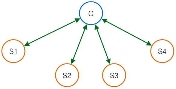
(a) Star message flow topology

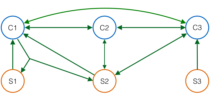
(b) A generic message flow topology where one of the streams originating at C1 has two subscribers: S1 and S2.

Figure 1: Information flow topologies

The protocol in this paper (“XOR-CoW”) targets a local wireless domain where nominally all nodes are in range, but fading might cause a pair of nodes to be unable to hear each other. The traffic patterns (referred to as “information topology”) considered are generic – any message ‘stream’ might have several destination nodes (called subscribers) and there are several such streams in a network. Within a short period of time (referred to as “cycle time”), every stream needs to deliver one packet reliably to each of its subscribers. The information topology can be arbitrary – something naturally centralized like a star topology as shown in Fig. 1(a) (e.g. with a central controller talking to many sensor/actuators collecting streams of measurements and sending streams of commands) or something more generic as in Fig. 1(b). The XOR-CoW protocol can support any arbitrary traffic but its performance peaks when the information topology is bi-directional (such as a star). This is due to the inherent two-way traffic that naturally facilitates opportunities for network coding.

The main contributions of this paper are as follows:

• A new protocol framework, called XOR-CoW, for applications that require ultra-reliable low-latency communication that combines cooperative communication and network coding.

• Analysis of the performance of XOR-CoW under a communication theoretic and delay-limited capacity framework.

• Comparison of various schemes’ (with and without network coding) performance by comparing the minimum SNR required to meet the QoS requirements.

• Optimization of the parameters of XOR-CoW to show that XOR-CoW is relatively insensitive to parameter choices. Most of the benefit comes from cooperative communication and network coding, so implementing more complicated schemes is not justified.

The rest of the paper is organized as follows. In Section II we first briefly review some of the recent trends in wireless communications, the evolution of communication for industrial control, cooperative communication, wireless diversity, and network coding techniques. For a more detailed treatment of the related work, please refer to [5]. Section III describes the resource assumptions and high level overview of Occupy CoW and XOR-CoW. Section IV and Section V describe the design of XOR-CoW framework in detail for generic traffic and bi-directional traffic, respectively. Section VI analyzes the performance of XOR-CoW and presents how it performs and compares it to hypothetical frequency-diversity-based scheme as well as cooperative communication scheme without network coding. Additionally, it presents how XOR-CoW protocol’s internal parameters can be optimized and discusses the implications for implementation. All the formulas used to generate the plots are derived in the Appendix.

II Background

II-A Recent development in $5$G protocols

The current vision of $5$G wireless standard not only focuses on increasing capacity and energy efficiency, but also on reducing latency. Tactile applications demanding latencies on the order of $1$ms may be enabled by using mmWave frequencies [7, 8]. Recent works like [9] concentrate on the proposed 5GETLA radio interface and show that latencies below $1$ ms for payloads of size $50$kb are achievable provided a bandwidth of 100MHz is available. Though the targeted latency is on the same order as required by industrial control, they do not consider reliability guarantees or retransmissions. The feasibility, requirements, and design challenges of an OFDM based 5G radio interface that is suitable for mission-critical MTC (machine type communication) is discussed in [10] where various modulation schemes as well as different MIMO configurations were considered. They concluded that for interference mitigation, multiple receive antennas were crucial. In similar spirit, the coverage and capacity aspects based on evaluations considering both noise-limited and interference-limited operations for MTC were considered in [11]. Several works have studied the suitability of various signaling strategies for low-latency applications. Specifically alternatives for OFDM have been considered to relax synchronization requirements and reduce out-of-band (OOB) transmissions such as Filter Bank Multi-carrier [12], Universal Filtered Multi-carrier [13] and Generalized Frequency Division Multiplexing [14]. In this paper, we do not consider explicit signaling strategies and push it for future work.

II-B Industrial Control

Communication in industrial control is supported by wired fieldbus systems like HART, PROFIBUS, WorldFIP, Foundation Fieldbus, and SERCOS [15] meet these requirements. Several wireless extensions of these fieldbus systems such as [16, 17] (as well as WirelessHART [18] and ISA100 [19]) which are based on wireless sensor network (WSN) techniques have been developed. They have worst-case latencies on the order of hundreds on milliseconds [20] making them unsuitable for high-performance control applications. WISA [21] targeted wireless control by employing frequency hopping techniques but it achieves latency on the order of $10$ms with a reliability of $10^{-4}$ [22], which fails to meet the reliability achieved by wired fieldbuses.

II-C Cooperative communication and multi-user diversity

In our prior work [5], we discussed some of the relevant references on cooperative communication and multi-user diversity in detail. Low-latency applications that we target cannot use time diversity since the cycle time can be shorter than the coherence time. Additionally, TDMA-based schemes for industrial control considered in [23, 24] do not scale well with network size. Commonly used frequency diversity techniques in WSN-inspired technologies [25] like channel hopping and contention-based MACs aren’t sufficient to obtain the required diversity as they cause unbounded delays. As there are multiple nodes in the system, harvesting cooperative, multi-user diversity is a viable option. Cooperation amongst distributed antennas can provide full diversity without physical arrays [26]. Even with noisy inter-user channels, multi-user cooperation increases capacity and leads to achievable rates that are robust to channel variations [27].

II-D Network Coding

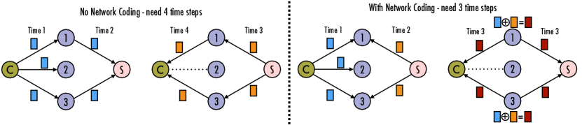
Figure 2: Illustration of network coding along with simultaneous retransmissions where the C and S nodes have information to convey to each other through 3 relays 1 - 3. The bold lines are active links and the dotted lines are inactive links. The blue packets are the downlink packets, the orange packets are the uplink packets and the maroon packets are the XORed packets. The XOR scheme can communicate the same amount of information in a shorter time because the uplink and downlink demands are satisfied simultaneously.

The seminal work of Ahlswede et al., [28] showed that regarding information to be multicast as a “fluid” to be routed or replicated in general is not optimal and employing coding at nodes can lead to efficient use of bandwidth. This idea was further studied in [29], where a forwarding architecture for wireless mesh networks to improve throughput by introducing a coding layer in between the IP and MAC layers was proposed. They provide a practical implementation of network coding into the current network stack, addressing the common case of unicast traffic, and dynamic and potentially bursty flows. Recent results in [30] show that using randomized space-time block coding (RSTBC) in two-way relay networks improves throughput by exchanging data through a bi-directional relay network. Like most works using network coding, we aim to increase throughput which translates to lower latency. Fig. 2 illustrates how we use network coding combined with simultaneous retransmissions in our work. Essentially, if there is a natural viability for XORing then, only those nodes with the necessary packets help by broadcasting the XORed packet.

The proposed wireless communication system combines cooperative communication and network coding techniques to achieve the desired QoS requirements by exploiting multi-user diversity and distributed space-time codes (such as those in [31, 32, 33], so that each receiver can harvest a large diversity gain) to achieve high-reliability and low latency. The key idea here is that relays simultaneously broadcast coded packets (as long as they are coding the same set of packets).

III Protocol Framework

The XOR-CoW protocol exploits multi-user diversity as well as side information at destination nodes by using simultaneous relaying combined with network coding to enable ultra-reliable communication. The general setup considered is that the network consists of $n$ nodes and each message stream (size $m$ bits) must reach its possibly many destinations within a cycle of time $T$. As we discussed in Section I, the information topology can be arbitrary.

III-A Resource assumptions

We make a few assumptions about the network, channel characteristics and hardware to abstract away some of the details and to support the exposition. These assumptions hold for all schemes discussed in this paper. The following assumptions are the same as the ones made in [5] for “Occupy CoW” protocol.

• We assume a local domain – that while normally, the nodes are within range of each other, bad fading events can cause transmissions to fail. Errors are caused only by bad fades.

• All nodes know the information topology. They share a universal addressing scheme and order. Messages are of the same size and they contain their destination addresses.

• Channels are assumed to be reciprocal. All nodes are half-duplex, but can switch instantly between transmit mode and receive mode.

• Channels are assumed to be quasi-static and remain the same during a cycle.

• Channel sounding to aid channel estimation is assumed to take a constant fraction of the cycle time $T$. All nodes are assumed to estimate channels that are being sounded. When multiple nodes simultaneously broadcast a message during the relaying phase, they would not need to spend time again sounding each channel and can do a short combined sounding as the intended receivers only need to identify which of the nodes that it can hear are transmitting.

• Clocks on each of the nodes are perfectly synchronized in both time and frequency. One could achieve adequate synchronization with low overhead by adapting techniques such as [34]. Thus we can schedule time slots for specific nodes without significant overhead.

• The protocol relies on time/frequency synchronization to achieve simultaneous retransmission of messages by multiple relays. We assume that if $k$ relays simultaneously (with consciously introduced timing jitter) transmit the exact same information, then all receivers can realize signal diversity $k$.

III-B Overview of Occupy CoW Protocol Framework

We briefly summarize the Occupy CoW protocol which would be the benchmark protocol for comparison purposes. For a detailed description, refer to [5]. The XOR-CoW protocol shares the same network setup and aims to meet the same requirements as Occupy CoW. In the Occupy CoW protocol, the source of different message streams transmit the message in a round-robin fashion. After all messages have been transmitted once, each message is then re-transmitted simultaneously by all the nodes which have the message (either the source or nodes that decoded the first transmission) using some appropriate distributed space-time code (DSTC) again in a round-robin fashion. Consider how this would play out for a star information topology as shown in Fig. 1(a). There is a downlink and uplink phase (corresponding to the first time the messages are transmitted) of length $T_{D_{1}}$ and $T_{U_{1}}$ respectively. This is followed by a scheduling phase where all “strong” nodes get to know the state of each message (whether it has reached the intended destination or not). This is followed by the relaying phases – first the downlink phases II (length $T_{D_{2}}$) and III (length $T_{D_{3}}$), where the controller and strong nodes alter the broadcast message to remove already-successful messages for the strong nodes and simultaneously broadcast the adapted packet. The unsuccessful nodes are listening. At the end of this phase, the nodes who received their messages from the controller have also received the global ACK information. which allows these nodes to participate as relays in the uplink phases. The uplink phases II (length $T_{U_{2}}$) and III (length $T_{U_{3}}$) are similar to their downlink counterparts. The protocol can either have two hops – such that there are only two downlink and uplink phases or three hops – where there are a total of three downlink phases and three uplink phases (as described above).

III-C Overview of XOR-CoW Protocol Framework

Consider two nodes (say A and B) that have messages to each other i.e., node A has a message for B and node B has a message for A. If the direct channel exists (link AB), then A’s message to B as well as B’s message to A succeeds in reaching the destination. If there is no direct channel, then A’s message to B may succeed if there is at least one node (say C) that has connection to both A and B. If there exists such a node, then both A’s message to B and B’s message to A succeeds via the same node (or set of nodes). Essentially, when there is a bi-directional traffic, the paths of ‘success’ in both direction are the same. When we have such bi-directional traffic patterns, then relay nodes can ‘XOR’ the packets and broadcast the resulting packet simultaneously using a DSTC as shown in Fig. 2. This is what we leverage in XOR-CoW – opportunistically network code packets. Network coding also provides throughput benefits (and as a result reduction in latency or reduction in SNR needed) when the traffic patterns are multicast (messages need to reach multiple destinations). We consider this scenario in detail in Section. IV.

IV XOR-CoW for Generic Information Topology

The XOR-CoW scheme for a generic information topology can be summarized as follows. All nodes know the information topology – the origin and destinations of the messages. Therefore, all nodes know which messages can be XORed. The schedule of messages $\mathcal{G}$ are determined and all nodes know the schedule. For the first phase, the schedule is simple: each message stream is allocated one slot. However, in the second phase (XOR phase), the schedule $\mathcal{G}_{X}$ is different: whenever bi-directional traffic exists in the information topology, allocate one slot for those two messages in $\mathcal{G}_{X}$, else allocate one slot for that single message in $\mathcal{G}_{X}$ (as shown in Fig. 3(a)). In the first phase, nodes take turn according to the schedule to transmit the messages. All nodes listen when they are not transmitting. In the XOR phase, all nodes that can transmit a message (or an XORed message) transmit according to the XOR phase schedule simultaneously using a DSTC. In the following section, we focus on the star topology as network coding yields maximum benefits when the traffic is bi-directional [35, 36].

V XOR-CoW for Bi-directional Information Topology

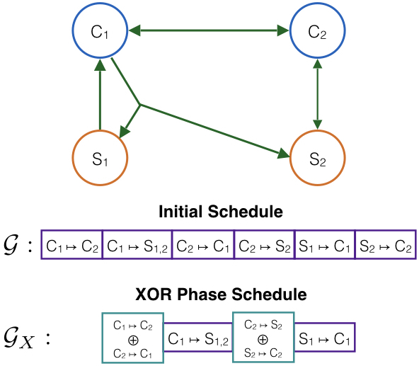
(a) Schedule during first phase and the XOR phase for a generic topology. Pairs of message streams that are inherently bi-directional i.e, $(C_{1}-C_{2},C_{2}-C_{1})$ and $(C_{2}-S_{2},S_{2}-C_{2})$ are the only ones that are XORed (shown in teal colored boxes).

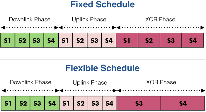
(b) Fixed and flexible scheduling for the star topology example considered in Fig. 4. The green boxes correspond to the downlink packets from the controller to the client nodes (the destinations are labelled: $\text{S}_{i}$). The pink boxes correspond to the uplink packets from the client nodes to the controller (the origins are labelled). The purple boxes correspond to the XOR packets where the label corresponds to client node whose DL and UL packets are XORed.

Figure 3: Scheduling for generic and star topology

In this section, we consider bi-directional topologies wherein if a node A has information for node B, then node B also has information for node A. A simple case of bi-directional traffic is the star topology which we will consider here for exposition purposes. A centralized control system can be modeled as a star topology where the network consists of a central controller $C$ and $n$ client nodes. In each ‘cycle’ of time $T$, the controller has $m$ distinct bits of message for each client node (downlink messages - DL) and each client node has $m$ distinct bits of message for the controller (uplink messages - UL). As in [5], we assume that while normally, the controller and all the nodes are in-range of each other, bad fading events can cause transmissions to fail. Successful nodes, namely those that have received both the downlink message from the controller and the uplink message for a client node in need, XOR the uplink and downlink messages together to form a single packet. They then broadcast the XORed packet simultaneously. The controller uses the XORed packet as well as the downlink information that it already has to decode the uplink packet. The destination node uses the XORed packet as well as the uplink information that it already has to decode its downlink packet.

This scheme has three phases: downlink phase, followed by uplink phase and then the XOR phase. Let the time allocated for the downlink phase be $T_{D}$, the uplink phase be $T_{U}$ and the XOR phase be $T_{X}$ such that $T_{D}+T_{U}+T_{X}=T$. We will describe the protocol with the aid of Fig. 4 where the network consists of one controller and $4$ nodes (S1 - S4). To the left of the figure are the downlink buffers at each node (controller and clients) and to the right of the figure are the uplink buffers, also at each node. They get populated as messages are decoded. Initially, the controller’s downlink buffer is full as it is the origin of all downlink messages (shown by the striped buffers) and its uplink buffer is empty. S1 - S4 start with their corresponding uplink buffer being full (shown by the striped buffers) and their downlink buffers are empty. The starred messages are those that each user is interested in receiving. The controller is interested in the uplink messages of nodes and the nodes are interested in receiving the specific downlink message intended for them.

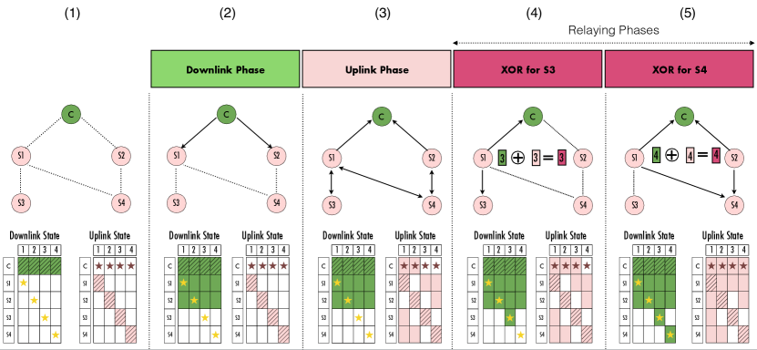
Figure 4: Simple example of XOR-CoW with one controller and 4 nodes. The graph illustrates which links are active during that phase. The downlink and uplink tables at each stage represent the information each node has at the end of that phase. Striped cells indicate message origins and starred cells indicate message destinations.

Schedules:
There are two versions of the XOR-CoW protocol that can be employed: a) fixed schedule protocol and b) flexible schedule protocol. The difference between these two mainly lies in the relaying phase – do all nodes get another shot at getting their message across or only those in need? This is illustrated in Fig. LABEL:fig:star-schedule. 1) Fixed schedule: In this scheme, time is allocated equally for all nodes in the XOR phase – such that they get another shot at sending their messages. Since the schedule is predetermined, the time at which the message of a particular node is to be transmitted is also known to all users and there is no real need for a scheduling phase to determine the schedule for the XOR phase.
2) Flexible schedule: In this scheme, time is allocated equally only for the nodes which need help in the XOR phase (and no time is given for the messages that have already reached the destination). This scheme requires a scheduling phase since the relays need to be told about the nodes that need help.
Keeping these schemes in mind, we describe the protocol under these schemes.

V-A Downlink and Uplink Phases

During these phases, all the nodes are listening whenever they are not transmitting. The downlink phase is common in both the fixed and flexible scheduling schemes. The cycle starts with a downlink phase in which the controller broadcasts a single packet consisting of all $m$-bit messages to all $n$ nodes at rate $R_{D}=\frac{m\cdot n}{T_{D}}$. In Fig 4 column 2, S1 and S2 successfully decode the entire downlink message. Their starred buffers are filled along with the downlink buffers corresponding to other nodes.
Fixed Schedule Scheme: This is followed by the uplink phase, in which the individual nodes transmit their messages to the controller one by one according to a predetermined schedule at rate $R_{U}=\frac{m}{T_{U}/n}=\frac{m\cdot n}{T_{U}}$ by evenly dividing the time slots among all nodes. In Fig 4 column 3, the controller successfully decodes the uplink messages of S1 and S2 and the starred uplink buffers of the controller corresponding to these nodes are filled. Since all nodes are listening whenever they are not transmitting, S1 receives the uplink messages of S3 and S4 while S2 receives the uplink message of S4. The nodes which have successfully received the downlink message as well as successfully transmitted their uplink message to the controller are referred to as strong nodes. In Fig. 4, S1 and S2 are the strong nodes.
Flexible Schedule Scheme: In the uplink phase of the flexible scheduling scheme, the nodes also transmit a one bit ACK to the controller (indicating whether they’ve successfully received the downlink packet or not). Therefore, the individual nodes transmit their messages (including one bit for an ACK) to the controller one by one according to a predetermined schedule at rate $R_{U}=\frac{m+1}{T_{U}/n}=\frac{(m+1)\cdot n}{T_{U}}$ by evenly dividing the time slots among all nodes.

V-B Scheduling Phase

This phase is crucial when the flexible scheduling scheme is employed. In this phase the controller transmits acknowledgments to the strong nodes (at the same rate as the downlink phase). This is just $2$ bits of information per node for downlink and uplink. The common-information about the system’s state enables the strong nodes to share a common schedule for relaying messages for the remaining nodes. Note that the schedule only reaches the strong nodes but the nodes which need help do not know the schedule. How will they know which message is intended for them without the knowledge of the schedule? This can be addressed by building in identification of the destination node in the packet such that the nodes can figure out which packet was addressed to them while keeping the transmission rate the same. This approach has been discussed in detail in [37]. Thus, for the remainder of the paper we’ll assume that the nodes know which packet was meant for them.

V-C XOR phase:

Depending on the scheduling scheme, the time allocated for this phase can either be equally divided among all nodes – corresponding to the rate of transmission is $R_{X}=\frac{m\cdot n}{T_{X}}$, or only those that need help – corresponding to the rate of transmission is $R_{X}=\frac{m\cdot n_{1}}{T_{X}}$ where $n_{1}$ are the number of unsuccessful nodes. In either case, the strong nodes XOR the downlink and uplink messages of each of the unsuccessful nodes they’ve heard. During the slot of an unsuccessful node (say node $Y$), all the strong nodes that have successfully heard node $Y$ act as simultaneous broadcast relays and transmit the XORed packet using a DSTC.

In Fig. 4, S3 and S4 are the unsuccessful nodes. In the XOR slot allocated for S3 (Fig. 4 column 3), S1 XORs the downlink and uplink packet of S3 (represented by the purple packet) and broadcasts it. Using the downlink packet of S3, the controller can now recover the uplink packet. Using its own uplink packet, S3 can now recover the downlink packet. The process for S4 is similar and the difference lies in the fact that S1 and S2 simultaneously transmit the XORed packet for S4.

VI Analysis of XOR-CoW

In this section, we analyze the performance of XOR-CoW. The performance of XOR-CoW’s performance for a generic information topology is the same as the performance of Occupy CoW for a generic topology. Therefore, we refer the readers to [5] for the analysis and performance of XOR-CoW when the traffic is not strictly bi-directional. In this paper, we focus on the performance of XOR-CoW for star topology only as we reap maximum benefits in this case.

VI-A Behavioral assumptions for analysis

Our analysis depends on the following behavioral assumptions in addition to the resource assumptions in Sec. III-A. We assume a fixed nominal SNR on all links with independent Rayleigh fading on each link. We also assume channel reciprocity. Our model assumes a single-tap channel (hence flat-fading). Because the cycle-time is so short, we use the delay-limited-capacity framework [38, 39].

A link with channel coefficient $h$ and bandwidth $W$ is deemed good (thus no errors or erasures) if the rate of transmission $R$ is less than or equal to the link’s capacity $C=W\log(1+|h|^{2}\textit{SNR})$. Consequently, the probability of link failure is defined as $p_{\scriptscriptstyle link}=P(R>C)=1-\exp{\left(-\frac{2^{R/W}-1}{\textit{SNR}}\right)}$.

As in [4], if there are $k$ simultaneous transmissions, then each receiver harvests perfect sender diversity of $k$. For analysis, this is treated as $k$ independent tries that only fail in communicating the message if all the tries fail. We do not consider any dispersion-style finite-block-length effects on decoding. This can be justified in spirit by [40]. We assume that transmission related errors are always detected  [41].

VI-B XOR-CoW probability of failure

The complete analysis of the performance of the XOR-CoW protocol is described in the VII. In this section we mainly present the results and state two theorems which are useful in understanding the results.

Theorem 1

If an instance of fixed schedule two-hop Occupy CoW protocol (i.e., no rate adaptation in the relaying phases) with equal downlink and uplink phases ($T_{D_{1}}=T_{U_{1}}=T_{D_{2}}=T_{U_{2}}=T_{M}$) succeeds, then there is a common downlink and uplink success path for each node in the network.

Proof:

If a node successfully decoded the downlink message in one hop, its uplink message also gets through successfully to the controller in one hop (due to channel reciprocity). If a node successfully decoded the downlink message in two hops via a relay $Z$, then the same relay helps uplink as well – again due to channel reciprocity. ∎

Theorem 2

If an instance of fixed schedule two-hop Occupy CoW protocol with equal downlink and uplink phase 1 ($T_{D_{1}}=T_{U_{1}}=T_{D_{2}}=T_{U_{2}}=T_{M}$) and a given SNR succeeds, then the fixed scheduling version of XOR-CoW with downlink and uplink phase lengths both equal to $T_{M}$ and XOR phase length also equals to $T_{M}$ succeeds at the same SNR.

Proof:

From Theorem 1 we know that the paths for downlink and uplink success when $T_{D_{1}}=T_{U_{1}}=T_{D_{2}}=T_{U_{2}}=T_{M}$ are the same – i.e., either they directly succeed to the controller or they have the same relay helping in both downlink and uplink. These relays essentially have the capability the XOR the packets as they have both the packets as well as good links for transmission. Hence, as long as the rate in the XOR phase stays the same (this is ensured by $T_{D}=T_{U}=T_{X}=T_{M}$), the XOR-CoW protocol also succeeds at the same SNR. ∎

A corollary of Theorem 2 is that while two-hop Occupy CoW would require time $4\times T_{M}$ to succeed, XOR-CoW succeeds in time $3\times T_{M}$ – i.e., a throughput improvement of $\frac{4}{3}$.

VI-C Results and comparison

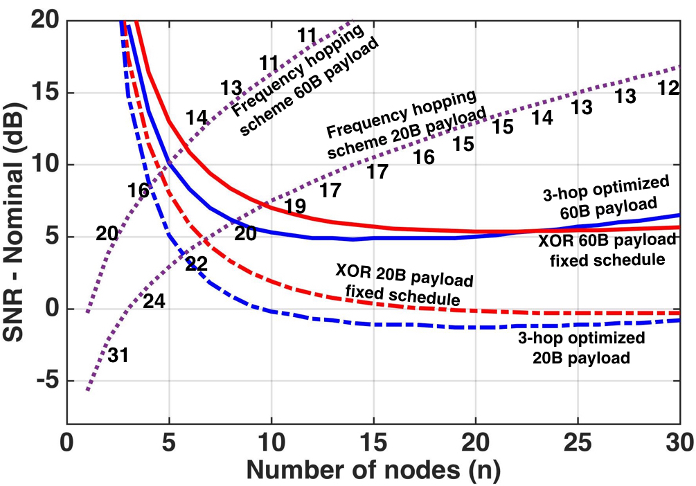
Figure 5: The performance of XOR-CoW for a star information topology compared with reference schemes for varying network size, and a $2$ms cycle time, aiming at $10^{-9}$ probability of failure for a $20$MHz channel. The numbers next to the frequency-hopping scheme show the frequency diversity needed and those next to the non-simultaneous retransmission scheme show the optimal number of relays per message stream.

We explore the performance of XOR-CoW with parameters taken from a contemporary practical application, the industrial printer case described in [2]. The SERCOS III protocol [42] supports the printer’s cycle time of $2$ ms with system error probability of $10^{-8}$. We target the following system requirements for the application: $30$ moving printing heads that move at speeds up to $3$ m/s over distances of up to $10$ m. Every cycle lasts $2$ms and in each cycle the controller transmits $20$ bytes of actuation data to each head and each of the $30$ sensors transmit $20$ bytes of sensory data to the controller. Assuming access to a single $20$MHz wireless channel, this $4.8$ Mbit/sec throughput corresponds to an overall spectral efficiency of approximately $0.25$ bits/sec/Hz. SERCOS supports a reliability of $10^{-8}$ and for our protocol we target a reliability of $10^{-9}$.

We define the cycle failure probability as the probability that any packet transmitted during the cycle did not reach at least one of its destinations. Following [4, 5] and the communication-theoretic convention, we use the minimum SNR required to achieve $10^{-9}$ reliability as our metric to compare XOR-CoW to other schemes. Fig. 5 compares the performance of the following protocols a) XOR-CoW, b) Occupy-CoW (the cooperative-communication-based protocol not employing network coding), and c) Frequency hopping based protocols. We see that optimized version of Occupy CoW (the best performance that can be obtained without using network coding) and XOR-CoW with a simple equal-time allocation to different phases perform comparably for $m=160$ bits (the dot-dashed lines). The advantage of XOR-CoW is clear for high aggregate rates and large networks as shown by the solid in Fig. 5. We see that XOR-CoW beats the performance of Occupy CoW for $m=480$ bits and network size $>20$ while also being a simpler scheme. The dotted purple curves represent a hypothetical (non-adaptive) frequency-hopping scheme that divides the bandwidth $W=20$MHz into $k$ sub-channels that are assumed to be independently faded, for $m=160$ bits and $m=480$ bits. The curves are annotated with the optimal $k$. As $k$ (and thus frequency hops) increases, the available diversity increases, but the added message repetitions force each link’s instantaneous data rate to be higher. For low $n$ the scheme prefers more frequency hops to exploit diversity benefits. The SNR cost of doing this is marginal because the throughput is low enough that we are still in the linear-regime of channel capacity. For networks with fewer than $7$ nodes, this says that using frequency-hopping is great — as long as we can reliably count on about $20$ independently faded sub-channels to repeat across, which is not always practical.

VI-D Optimization

VI-D1 Network Coding Optimization

XOR-CoW scheme only allows for the opportunity to XOR two packets and not more. Are we making sub-optimal decisions by restricting to XORing only two packets? We are not and the reason is as follows. In undirected network (wireless networks considered here can be modeled as undirected networks) the throughput improvement that network coding provides when compared to routing only schemes is upper bounded at $2$ [43]. We showed in Sec. VI that the throughput improvement for the best case i.e., the star-topology is actually $\frac{4}{3}<2$.

Furthermore, we can model the generic information topology as a multicast session. It has been shown that asymptotically network coding provides no benefits when compared to a pure routing schemes [44]. Additionally, even if we end up with a network realization which can provide significant network coding benefits (a rare event in itself), the coding points (which perform network coding operation) need to know the state of each packet and the network realization to compute the optimium code. The overhead of acquiring this network information state is significant (similar in spirit to why backpressure routing isn’t implemented as-is in current networks).

VI-D2 Phase Length Optimization

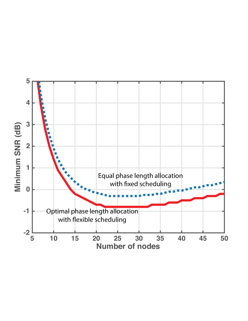
(a) SNR comparison of optimized flexile-schedule XOR-CoW and fixed-schedule XOR-CoW for $m=160$ bit and varying network size with $20$MHz bandwidth and a $2$ms cycle time, aiming at $10^{-9}$.

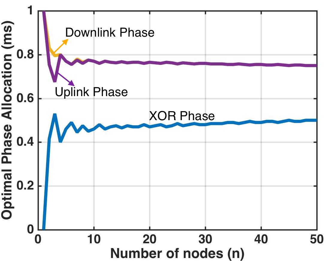
(b) The phase allocation for optimized XOR-CoW with flexible scheduling for $m=160$ bit messages and varying network size with $20$MHz bandwidth and a $2$ms cycle time, aiming at $10^{-9}$ is shown.

Figure 6: Optimization of XOR-CoW protocol

We consider the XOR-CoW protocol and look at the optimal allocation of time which minimizes the SNR required to meet the performance specifications. Although the phase length allocations are uneven (as seen in the figure 6(b)), we find that the SNR saving that we achieve by having different lengths is minimal (as seen in the figure 6(a)). The complexity of building a system which can operate at variable rates is extremely difficult and ultimately negates out the small SNR savings achieved by optimization. The strength of the protocol lies in the fact that a simple scheme with equal time allocations with fixed schedule performs almost as good as the optimal scheme – thus paving the way for a practical system.

VII Conclusions & Future Work

In this work, we designed a network coding based wireless communication protocol framework for high-performance control-like systems. We have additionally shown that simple phase length allocations are sufficient and optimizations only provide marginal benefits. In the future, we aim to address the impact of modeling assumptions such as spatial independence, quasi-static behavior, etc., on cooperative communication protocols. Understanding the impact of imperfect sychronization as well as imperfect channel estimation would also be important in making these schemes practical.

We analyze the XOR-CoW protocol by looking at all the ways at least one of the messages did not reach the destination within the cycle as in [5, 4]. We achieve this by partitioning the nodes into various sets which depend on various aspects like downlink/uplink success and the state of node-node as well as node-controller links in different phases. Before continuing with the analysis itself, we define some notation.

Notation

To effectively present the derived expressions, we provide a guide to the notation that will be used in the following sections. Let a transmission over a single link be an “experiment.” A binomial distribution with $n$ independent experiments, probability of success $1-p$, and number of success $m$ will be referred to as

$$B(n,m,p)=\binom{n}{m}(1-p)^{m}p^{n-m}.$$ (1)

Note that the probability $p$ is the probability of failure, not the probability of success. The probability of at least one out of $n$ independent experiments failing will be denoted as

$$F(n,p)=1-(1-p)^{n}.$$ (2)

A link with fading coefficient $h$ and bandwidth $W$ is considered “good” (thus decodable) if the rate of transmission $R_{i}$ is less than or equal to the link’s capacity, $C=W\log(1+|h|^{2}\text{SNR})$. We assume that the nominal operating SNR is held consistent across the entire system. Consequently, for a rate $R$, the assumption of Rayleigh fading tells us that the probability of an unsuccessful transmission is defined as

$$p=P(R>C)=1-\exp{\left(-\frac{2^{R/W}-1}{\text{SNR}}\right)}.$$ (3)

We assume that if $R$ exceeds capacity, the transmission will surely fail (with probability 1). If $R$ is less than capacity, the transmission will surely succeed and decode to the right codeword.

Set Notation

We describe the various sets used in the analysis. Following general convention, the set itself will be represented in script font. The random variable representing the number of nodes in that set will be presented in uppercase letters. Finally, the instantiation of that random variable (the cardinality of the set), will be in lowercase letters. The sets being considered are:

• $\mathcal{A}$: the set of nodes successful in the downlink phase. Further divided into disjoint sets $\widetilde{\mathcal{A}}$ and $\widecheck{\mathcal{A}}$ such that $\mathcal{A}=\widetilde{\mathcal{A}}\bigcup\widecheck{\mathcal{A}}$.

  • $\widetilde{\mathcal{A}}$: the set of nodes which succeed in downlink as well as uplink phases. This is further partitioned into $\widetilde{\mathcal{A}}_{X}$ (the set which connects to the controller in the XOR phase) and $\widetilde{\mathcal{A}}_{U}$ (the set which cannot connect to the controller in the XOR phase).

  • $\widecheck{\mathcal{A}}$: the set of nodes which do not succeed in uplink. This set is further partitioned into $\widecheck{\mathcal{A}}_{X}$ (which can connect to the controller in the XOR phase) and $\widecheck{\mathcal{A}}_{D}$ (which cannot connect to the controller in the XOR phase).

• $\mathcal{B}$: the set of nodes that weren’t successful in downlink phase but were successful in uplink phase. Further partitioned into disjoint sets $\widetilde{\mathcal{B}}$ (has link to the controller in the XOR phase) and $\widecheck{\mathcal{B}}$ (doesn’t have link to controller in the XOR phase) such that $\mathcal{B}=\widetilde{\mathcal{B}}\bigcup\widecheck{\mathcal{B}}$.

• $\mathcal{C}$: the set of nodes that succeed only in the XOR phase – both uplink and downlink successes happen in this phase. They can only succeed through relays.

Analysis of XOR-CoW:

Let the time allocated for the downlink phase be $T_{D}$, the uplink phase be $T_{U}$ and the XOR phase be $T_{X}$ such that $T_{D}+T_{U}+T_{X}=T$ where $T$ is the given cycle time. If we chose to do fixed scheduling then the transmission rates for downlink, uplink and XOR phases are fixed at $R_{D}=\frac{m\cdot n}{T_{D}}$, $R_{U}=\frac{m\cdot n}{T_{U}}$ and $R_{X}=\frac{m\cdot n}{T_{X}}$ respectively. If adaptive scheduling scheme is employed, then the transmission rates for downlink, uplink and XOR phases are given by $R_{D}=\frac{m\cdot n}{T_{D}}$, $R_{U}=\frac{(m+1)\cdot n}{T_{U}}$ and $R_{X}=\frac{m\cdot(n-\widetilde{a})}{T_{X}}$ where $\widetilde{a}$ is the number of nodes that succeeded in both uplink and downlink phases. These $\tilde{\mathcal{A}}$ are called “strong nodes” and all the others need help. Without loss of generality we consider the flexible schedule scheme and proceed with the analysis. Depending on the time allocations for different phases and the number of strong nodes $\widetilde{a}$, we get the following theorem.

Theorem 3

Let the time allocated for downlink, uplink and XOR phases be $T_{D}$, $T_{U}$ and $T_{X}$ respectively, the number of non-controller nodes be $n$, and message size be $m$ bits. The downlink and uplink transmission rates are given by $R_{D}=\frac{m\cdot n}{T_{D}}$ and $R_{U}=\frac{(m+1)\cdot n}{T_{U}}$ respectively. The corresponding probability of a single link failure, $p_{D}$ & $p_{U}$, is given by Eq. (3). The XOR phase transmission rate is given by $R_{X}^{\widetilde{a}}=\frac{m\cdot(n-\widetilde{a})}{T_{X}}$ where $\widetilde{a}$ is the number of “strong nodes” in both downlink and uplink phases and the corresponding probability of a single failure $p_{X}$, is given by Eq. (3). The probability XOR-CoW failure is then

$$\begin{aligned} P(\text{fail})&=\sum_{a=0}^{n}\Bigg{[}\sum_{b=0}^{n-a}P\left(\text{fail}_{1}\right)\mathds{1}\left(R_{D}\geq R_{U}>R_{X}\right)+\sum_{b=0}^{n-a}\sum_{\widetilde{b}=0}^{b}P\left(\text{fail}_{2}\right)\mathds{1}\left(R_{D}>R_{X}\geq R_{U}\right)\\ &\hskip 30.0pt+\sum_{\widetilde{a}=0}^{a}P\left(\text{fail}_{3}\right)\mathds{1}\left(R_{U}\geq R_{D}>R_{X}\right)+\sum_{\widetilde{a}=0}^{a}\sum_{\widecheck{a}_{X}=0}^{a-\widetilde{a}}P\left(\text{fail}_{4}\right)\mathds{1}\left(R_{U}>R_{X}\geq R_{D}\right)\\ &\hskip 30.0pt+\sum_{\widetilde{a}=0}^{a}\sum_{\widetilde{a}_{X}=0}^{\widetilde{a}}P\left(\text{fail}_{5}\right)\mathds{1}\left(R_{X}\geq R_{U}>R_{D}\right)+\sum_{\widetilde{a}_{X}=0}^{a}\sum_{b=0}^{n-a}P\left(\text{fail}_{6}\right)\mathds{1}\left(R_{X}>R_{D}\geq R_{U}\right)\Bigg{]}\end{aligned}$$

where, $P\left(\text{fail}_{1}\right)=B(n,a,p_{D})\times B(n-a,b,q_{UD})\times F(n-a-b,p_{U}^{a})$
is the probability of failure if the relationship between the rates is $R_{D}\geq R_{U}>R_{X}$,

$$P\left(\text{fail}_{2}\right)=B(n,a,p_{D})\times B(n-a,b,q_{UD})\times B(b,\widetilde{b},r_{UX,UD})\times F(n-a-\widetilde{b},p_{X}^{a})$$

is the probability of failure if the relationship between the rates is $R_{D}>R_{X}\geq R_{U}$,

$$P\left(\text{fail}_{3}\right)=B(n,a,p_{D})\times B(a,\widetilde{a},s_{UD})\times F(n-a,p_{U}^{a})$$

is the probability of failure if the relationship between the rates is $R_{U}\geq R_{D}>R_{X}$,

$$P\left(\text{fail}_{4}\right)=B(n,a,p_{D})\times B(a,\widetilde{a},s_{UD})\times B(\widecheck{a},\widecheck{a}_{X},r_{DX,DU})\times F(n-\widetilde{a}-\widecheck{a}_{X},p_{U}^{\widetilde{a}+\widecheck{a}_{X}})$$

is the probability of failure if the relationship between the rates is $R_{U}>R_{X}\geq R_{D}$,

$$P\left(\text{fail}_{5}\right)=B(n,a,p_{D})\times B(a,\widetilde{a},s_{UD})\times B(\widetilde{a},\widetilde{a}_{X},s_{XU})\times(1-P(\text{success}_{5}))$$

$$P(\text{success}_{5})=(1-p_{X}^{\widetilde{a}_{X}})^{\widecheck{a}}\times\left(\sum_{k=1}^{\widetilde{a}_{X}}B(\widetilde{a}_{X},k,p_{U})\left(1-s_{XU}^{k}+s_{XU}^{k}(1-p_{X}^{\widetilde{a}_{U}})\right)\right)^{n-a}$$

are the probabilities of failure and success if the relationship between the rates is $R_{X}\geq R_{U}>R_{D}$, $P\left(\text{fail}_{6}\right)=B(n,a,p_{D})\times B(\widetilde{a},\widetilde{a}_{X},s_{XD})\times B(n-a,b,q_{UD})\times(1-P(\text{success}_{6}))$

$$P(\text{success}_{6})=(1-p_{X}^{a})^{b}\times\left(\sum_{k=1}^{\widetilde{a}_{X}}B(\widetilde{a}_{X},k,p_{U})\left(1-s_{XU}^{k}+s_{XU}^{k}(1-p_{X}^{\widetilde{a}_{U}})\right)\right)^{n-a-b}$$

are the probabilities of failure and success if the relationship between the rates is $R_{X}>R_{D}\geq R_{U}$, where:

• $q_{UD}=P(C<R_{U}|C<R_{D})=\frac{p_{U}}{p_{D}}$

• $s_{UD}=P(C<R_{U}|C>R_{D})=\frac{p_{U}-p_{D}}{1-p_{D}}$

• $s_{XU}=P(C<R_{X}|C>R_{U})=\frac{p_{X}-p_{U}}{1-p_{U}}$

• $s_{XD}=P(C<R_{X}|C>R_{D})=\frac{p_{X}-p_{D}}{1-p_{D}}$

• $r_{UX,UD}=P(R_{U}<C<R_{X}|R_{U}<C<R_{D})=\frac{p_{X}-p_{U}}{p_{D}-p_{U}}$

• $r_{DX,DU}=P(R_{D}<C<R_{X}|R_{D}<C<R_{U})=\frac{p_{X}-p_{D}}{p_{U}-p_{D}}$

Proof:

All potential relays get the schedules in the scheduling phase where the rate of transmission is the same as downlink rate as stated earlier in Sec. III. This ensures that all potential relays (those that have the downlink information) know when to transmit. Additionally, all nodes that need help also know which packet is intended for them as their identity is built into the packet. We look at each case to understand the subtle effects that may arise.

(a) Case 1: $R_{D}\geq R_{U}>R_{X}$.

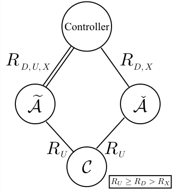
(b) Case 2: $R_{U}\geq R_{D}>R_{X}$.

Figure 7: Different ways to succeed in XOR-CoW protocol. The links between the controller and nodes are annotated with the rates in which they are present. The links to $\mathcal{C}$ are only denoted for the rate at which the links are important.

Case 1: $R_{D}\geq R_{U}>R_{X}$
The rates of transmission are as described earlier and the probabilities of a link succeeding in downlink, uplink and XOR phases are given by $p_{D}$, $p_{U}$ and $p_{X}$ respectively. Fig. 7(a) shows the exhaustive list of ways to succeed in the first case of the XOR-CoW protocol.

• A node can succeed directly to the controller in downlink – these nodes are in set $\mathcal{A}$. As the rate in downlink phase $R_{D}$ is greater than the rate in uplink phase $R_{U}$, these nodes also succeed in uplink directly to the controller (so they are an overall success). In this case, $\widetilde{\mathcal{A}}=\mathcal{A}$ as all of $\mathcal{A}$ retain links in the uplink phase and they are potential relays.

• A node can gain a link to the controller at the lower uplink rate of $R_{U}$ – these nodes are in set $\mathcal{B}$. They get their downlink message directly from the controller in the XOR phase as all of them retain the link to the controller in the XOR phase.

• A node can have both downlink and uplink successes during the XOR phase, if they connected to $\mathcal{A}$ in the uplink phase and as the rate $R_{X}$ in the XOR phase is less than $R_{U}$, the links do not disappear.

To calculate the probability of error of the XOR-CoW protocol, we will unroll the state space and sum over all possible instantiations of the sets of interest that result in failure. The probability of $A=a$ depends on the point to point link to the controller which has a failure probability of $p_{D}$ (we use Eq. (3)). Thus we have $P(A=a)=B(n,a,p_{D})$. The probability that a node does not gain a link to the controller in the uplink phase given it did not have a link in the downlink phase is given by $q_{UD}=P(C<R_{U}|C<R_{D})=p_{U}/p_{D}$. Conditioned on the realization that $A=a$, the probability that $B=b$ nodes gain links to the controller is given by $P(B=b|A=a)=B(n-a,b,q_{UD})$.

Given $A=a$ and $B=b$, the probability of a node in $\mathcal{S}\setminus\left(\mathcal{A}\bigcup\mathcal{B}\right)$, failing in the XOR phase is the probability that it doesn’t connect to $\mathcal{A}$ in the uplink phase. The probability of a single node failing is given by $p_{U}^{a}$. Thus the overall probability of failure given $A=a$ and $B=b$ is $F(n-a-b,p_{U}^{a})$. Thus we get that the probability of failure of the XOR-CoW protocol when the relationship between the rates is $R_{D}\geq R_{U}>R_{X}$ is given by

$$\sum_{a=0}^{n}\sum_{b=0}^{n-a}P\left(\text{fail}_{1}\right)\mathds{1}\left(R_{D}\geq R_{U}>R_{X}\right)$$

where, $P\left(\text{fail}_{1}\right)=B(n,a,p_{D})\times B(n-a,b,q_{UD})\times F(n-a-b,p_{U}^{a}).$

Case 2: $R_{U}\geq R_{D}>R_{X}$
The rates of transmission are as described earlier and the probabilities of a link succeeding in downlink, uplink and XOR phases are given by $p_{D}$, $p_{U}$ and $p_{X}$ respectively. Fig. 7(b) shows the exhaustive list of ways to succeed in the third case of the XOR-CoW protocol.

• A node can succeed directly to the controller in downlink – these nodes are in set $\mathcal{A}$. As the rate $R_{D}$ in the downlink phase is lower than the rate $R_{U}$ in the uplink phase, this set is further divided into two disjoint sets $\widetilde{\mathcal{A}}$ (which retains the connection to the controller in the uplink phase) and $\widecheck{\mathcal{A}}$ (which loses the connection to the controller in the uplink phase). The nodes in $\widetilde{\mathcal{A}}$ are the potential uplink message helpers in the XOR phase.

• The nodes in $\widecheck{\mathcal{A}}$ succeed directly to the controller in the XOR phase as they have the downlink as well as uplink packets to XOR.

• A node can have both downlink and uplink successes during the XOR phase, if they connected to $\mathcal{A}$ in the uplink phase and as the rate in XOR phase $R_{X}$ is less than $R_{U}$, the links do not disappear.

To calculate the probability of error of the XOR-CoW protocol, we will unroll the state space and sum over all possible instantiations of the sets of interest that result in failure. The probability of $A=a$ depends on the point to point link to the controller which has a failure probability of $p_{D}$ (we use Eq. (3)). Thus we have $P(A=a)=B(n,a,p_{D})$. Given $A=a$, the probability that a node in $\mathcal{A}$ loses its link to the controller in the uplink phase is given by $s_{UD}=P(C<R_{U}|C>R_{D})=(p_{U}-p_{D})/(1-p_{D})$. Thus we get the probability that $\widetilde{A}=\widetilde{a}$ (these do not lose the links) given $A=a$ is $B(a,\widetilde{a},s_{UD})$. Given $A=a$ and $\widetilde{A}=\widetilde{a}$, the probability of a node in $\mathcal{S}\setminus\mathcal{A}$, failing in the XOR phase is the probability that it doesn’t connect to $\mathcal{A}$ in the uplink phase. The probability of a single node failing is given by $p_{U}^{a}$. Thus, the overall probability of failure given $A=a$ and $\widetilde{A}=\widetilde{a}$ is $F(n-a,p_{U}^{a})$. Thus, we get that the probability of failure of the XOR-CoW protocol when the relationship between the rates is $R_{U}\geq R_{D}>R_{X}$ is given by

$$\sum_{a=0}^{n}\sum_{\widetilde{a}=0}^{a}P\left(\text{fail}_{3}\right)\mathds{1}\left(R_{U}\geq R_{D}>R_{X}\right)$$

where, $P\left(\text{fail}_{3}\right)=B(n,a,p_{D})\times B(a,\widetilde{a},s_{UD})\times F(n-a,p_{U}^{a}).$

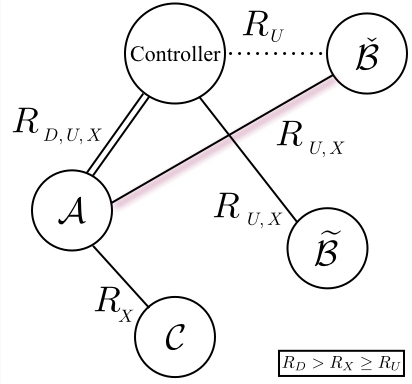
(a) Case 3: $R_{D}>R_{X}\geq R_{U}$.

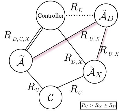
(b) Case 4: $R_{U}>R_{X}\geq R_{D}$.

Figure 8: Different ways to succeed in XOR-CoW protocol. The links between the controller and nodes are annotated with the rates in which they are present. The links to $\mathcal{C}$ are only denoted for the rate at which the links are important.

Case 3: $R_{D}>R_{X}\geq R_{U}$
The rates of transmission are as described earlier and the probabilities of a link succeeding in downlink, uplink and XOR phases are given by $p_{D}$, $p_{U}$ and $p_{X}$ respectively. Fig. 8(a) shows the exhaustive list of ways to succeed in the second case of the XOR-CoW protocol.

• A node can succeed directly to the controller in downlink – these nodes are in set $\mathcal{A}$. As the rate in downlink phase $R_{D}$ is greater than the rate in uplink phase $R_{U}$, these nodes also succeed in uplink directly to the controller (they are an overall success). In this case $\widetilde{\mathcal{A}}=\mathcal{A}$ as all nodes in $\mathcal{A}$ retain links in uplink phase. All of these will be potential relays.

• A node can gain a link to the controller at the lower uplink rate of $R_{U}$ – these nodes are in the set $\mathcal{B}$. Some of these nodes lose the link during the XOR phase as (since $R_{X}\geq R_{U}$). The nodes that retain the links constitute the set $\widetilde{\mathcal{B}}$ and the ones which lose the link constitute the set $\widecheck{\mathcal{B}}$. The set $\widetilde{\mathcal{B}}$ get their downlink message directly from the controller in the XOR phase but the set $\widecheck{\mathcal{B}}$ doesn’t. They need to connect to at least one node in $\mathcal{A}$ in the uplink as well as XOR phase to successfully receive their downlink message.

• A node can have both downlink and uplink successes during the XOR phase, if they connected to $\mathcal{A}$ in the uplink phase as well as in the XOR phase (similar to $\widecheck{\mathcal{B}}$).

To calculate the probability of error of the XOR-CoW protocol, we will unroll the state space and sum over all possible instantiations of the sets of interest that result in failure. The probability of $A=a$ depends on the point to point link to the controller which has a failure probability of $p_{D}$ (we use Eq. (3)). Thus we have $P(A=a)=B(n,a,p_{D})$. The probability that a node does not gain a link to the controller in the uplink phase given it did not have a link in the downlink phase is given by $q_{UD}=P(C<R_{U}|C<R_{D})=p_{U}/p_{D}$. Conditioned on the realization that $A=a$, the probability that $B=b$ nodes gain link to the controller is given by $P(B=b|A=a)=B(n-a,b,q_{UD})$. Given $B=b$, the probability that a node in $\mathcal{B}$, loses the connection to the controller in the XOR phase is given by $r_{UX,UD}=p(R_{U}<C<R_{X}|R_{C}<C<R_{D})=(p_{X}-p_{U})/(p_{D}-p_{U})$. Thus the probability that $\widetilde{B}=\widetilde{b}$ given $B=b$ is given by $B(b,\widetilde{b},r_{UX,UD})$. Given $A=a$, $B=b$ and $\widetilde{B}=\widetilde{b}$ the probability of a node in $\mathcal{S}\setminus\left(\mathcal{A}\bigcup\widetilde{\mathcal{B}}\right)$, failing in the XOR phase is the probability that it doesn’t connect to $\mathcal{A}$ in the uplink and XOR phases. The probability of a single node failing is given by $p_{X}^{a}$. Thus, the overall probability of failure given $A=a$, $B=b$ and $\widetilde{B}=\widetilde{b}$ is $F(n-a-\widetilde{b},p_{X}^{a})$. Thus, we get that the probability of failure of the XOR-CoW protocol when the relationship between the rates is $R_{D}>R_{X}\geq R_{U}$ is given by

$$\sum_{a=0}^{n}\sum_{b=0}^{n-a}\sum_{\widetilde{b}=0}^{b}P\left(\text{fail}_{2}\right)\mathds{1}\left(R_{D}>R_{X}\geq R_{U}\right)$$

where, $P\left(\text{fail}_{2}\right)=B(n,a,p_{D})\times B(n-a,b,q_{UD})\times B(b,\widetilde{b},r_{UX,UD})\times F(n-a-\widetilde{b},p_{X}^{a}).$

Case 4: $R_{U}>R_{X}\geq R_{D}$
The rates of transmission are as described earlier and the probabilities of a link succeeding in downlink, uplink and XOR phases are given by $p_{D}$, $p_{U}$ and $p_{X}$ respectively. Fig. 8(b) shows the exhaustive list of ways to succeed in the fourth case of the XOR-CoW protocol.

• A node can succeed directly to the controller in downlink – these nodes are in set $\mathcal{A}$. As the rate in downlink phase $R_{D}$ is lower than the rate in uplink phase $R_{U}$, this set is further divided into two disjoint sets $\widetilde{\mathcal{A}}$ (which retains the connection to the controller in the uplink phase) and $\widecheck{\mathcal{A}}$ (which loses the connection to the controller in the uplink phase).

• The nodes in $\widecheck{\mathcal{A}}$ are further divided to $\widecheck{\mathcal{A}}_{X}$ (those that regain the link to the controller in the XOR phase) and $\widecheck{\mathcal{A}}_{D}$ (those that do not regain the link to the controller). The nodes in $\widecheck{\mathcal{A}}_{X}$ successfully transmit their own uplink message to the controller in the XOR phase as they have the downlink messages to XOR and the link to transmit.

• The nodes in $\widecheck{\mathcal{A}}_{D}$ succeed only by connecting to $\widetilde{\mathcal{A}}\bigcup\widecheck{\mathcal{A}}$ in the uplink phase (the link back to them will automatically exist in the XOR phase since $R_{X}<R_{U}$).

• Any other node can have both downlink and uplink successes during the XOR phase, if they connected to $\widetilde{\mathcal{A}}\bigcup\widecheck{\mathcal{A}}_{X}$ in the uplink phase and as the rate in XOR phase $R_{X}$ is less than $R_{U}$, the links do not disappear.

To calculate the probability of error of the XOR-CoW protocol, we will unroll the state space and sum over all possible instantiations of the sets of interest that result in failure. The probability of $A=a$ depends on the point to point link to the controller which has a failure probability of $p_{D}$ (we use Eq. (3)). Thus we have $P(A=a)=B(n,a,p_{D})$. Given $A=a$, the probability that a node in $\mathcal{A}$ loses link to the controller in the uplink phase is given by $s_{UD}=P(C<R_{U}|C>R_{D})=(p_{U}-p_{D})/(1-p_{D})$. Thus we get the probability that $\widetilde{A}=\widetilde{a}$ (these do not lose the links) given $A=a$ is $B(a,\widetilde{a},s_{UD})$. Given $A=a$ and $\widetilde{A}=\widetilde{a}$, the probability of a node in $\widecheck{\mathcal{A}}$ gaining a link to the controller in the XOR phase is given by $1-P(R_{D}<C<R_{X}|R_{D}<C<R_{U})=1-r_{DX,DU}$. Thus, we get that $\widecheck{A}_{X}=\widecheck{a}_{X}$ nodes gain links to the controller in the XOR phase with probability $B(\widecheck{a},\widecheck{a}_{X},r_{DX,DU})$.

Given $A=a$, $\widetilde{A}=\widetilde{a}$ and $\widetilde{A}_{X}=\widetilde{a}_{X}$, the probability of a node in $\mathcal{S}\setminus\left(\widetilde{\mathcal{A}}\bigcup\widecheck{\mathcal{A}}_{X}\right)$ failing in the XOR phase is the probability that it doesn’t connect to $\widetilde{\mathcal{A}}\bigcup\widecheck{\mathcal{A}}_{X}$ in the uplink phase. The probability of a single node failing is given by $p_{U}^{\widetilde{a}+\widecheck{a}_{X}}$. Thus the overall probability of failure given $A=a$ and $\widetilde{A}=\widetilde{a}$ is $F(n-\widetilde{a}-\widecheck{a}_{X},p_{U}^{\widetilde{a}+\widecheck{a}_{X}})$. Thus we get that the probability of failure of the XOR-CoW protocol when the relationship between the rates is $R_{U}>R_{X}\geq R_{D}$ is given by

$$\sum_{a=0}^{n}\sum_{\widetilde{a}=0}^{a}\sum_{\widecheck{a}_{X}=0}^{a-\widetilde{a}}P\left(\text{fail}_{4}\right)\mathds{1}\left(R_{U}>R_{X}\geq R_{D}\right)$$

where, $P\left(\text{fail}_{4}\right)=B(n,a,p_{D})\times B(a,\widetilde{a},s_{UD})\times B(\widecheck{a},\widecheck{a}_{X},r_{DX,DU})\times F(n-\widetilde{a}-\widecheck{a}_{X},p_{U}^{\widetilde{a}+\widecheck{a}_{X}}).$

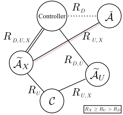
(a) Case 5: $R_{X}\geq R_{U}>R_{D}$.

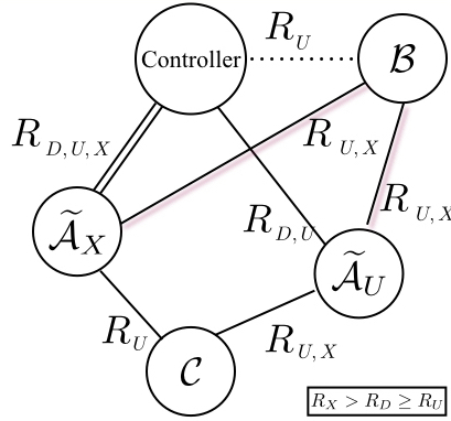
(b) Case 6: $R_{X}>R_{D}\geq R_{U}$.

Figure 9: Different ways to succeed in XOR-CoW protocol. The links between the controller and nodes are annotated with the rates in which they are present. The links to $\mathcal{C}$ are only denoted for the rate at which the links are important.

Case 5: $R_{X}\geq R_{U}>R_{D}$
The rates of transmission are as described earlier and the probabilities of a link succeeding in downlink, uplink and XOR phases are given by $p_{D}$, $p_{U}$ and $p_{X}$ respectively. Fig. 9(a) shows the exhaustive list of ways to succeed in the fifth case of the XOR-CoW protocol.

• A node can succeed directly to the controller in downlink – these nodes are in set $\mathcal{A}$. As the rate in downlink phase $R_{D}$ is lower than the rate in uplink phase $R_{U}$, this set is further divided into two disjoint sets $\widetilde{\mathcal{A}}$ (which retains the connection to the controller in the uplink phase) and $\widecheck{\mathcal{A}}$ (which loses the connection to the controller in the uplink phase).

• The nodes in $\widetilde{\mathcal{A}}$ are further divided to $\widetilde{\mathcal{A}}_{X}$ (those that retain the link to the controller in the XOR phase – thus can act as uplink message relays) and $\widetilde{\mathcal{A}}_{U}$ (those that lose the link to the controller). The set $\widetilde{\mathcal{A}}_{U}$ can still act a relays for downlink messages.

• The nodes in $\widecheck{\mathcal{A}}$ succeed only if they connect to $\widetilde{\mathcal{A}}_{X}$ in the uplink phase.

• The nodes in $\mathcal{S}\setminus\mathcal{A}$ succeed only in the following way: they must connect to $\widetilde{\mathcal{A}}_{X}$ in the uplink phase (to convey their uplink message). They can receive their downlink message either by connecting to $\widetilde{\mathcal{A}}_{X}$ in the XOR phase (this is not guaranteed as the rate in the XOR phase is higher) or by connecting to $\widetilde{\mathcal{A}}_{U}$ in the uplink and XOR phase.

To calculate the probability of error of the XOR-CoW protocol, we will unroll the state space and sum over all possible instantiations of the sets of interest that result in failure. The probability of $A=a$ depends on the point to point link to the controller which has a failure probability of $p_{D}$ (we use Eq. (3)). Thus we have $P(A=a)=B(n,a,p_{D})$. Given $A=a$, the probability that a node in $\mathcal{A}$ loses link to the controller in the uplink phase is given by $s_{UD}=P(C<R_{U}|C>R_{D})=(p_{U}-p_{D})/(1-p_{D})$. Thus we get the probability that $\widetilde{A}=\widetilde{a}$ (these do not lose the links) given $A=a$ is $B(a,\widetilde{a},s_{UD})$. Given $A=a$ and $\widetilde{A}=\widetilde{a}$, the probability that a node in $\widetilde{\mathcal{A}}$ loses link to the controller in the XOR phase is given by $s_{XU}=P(C<R_{X}|C>R_{U})=(p_{X}-p_{U})/(1-p_{U})$. Thus, the probability that $\widetilde{\mathcal{A}}_{X}=\widetilde{\mathcal{A}}_{X}$ is given by $B(\widetilde{a},\widetilde{a}_{X},s_{XU})$.

The probability that nodes in $\widecheck{\mathcal{A}}$ succeed is the probability that they connect to $\widetilde{\mathcal{A}}_{X}$ in the uplink phase which is given by $1-p_{U}^{\widetilde{a}_{X}}$. Thus the probability that all nodes in $\widecheck{\mathcal{A}}$ succeed is $(1-p_{U}^{\widetilde{a}_{X}})^{\widecheck{a}}$. For the rest of the nodes, let us calculate the probability of success. To succeed, a node must connect to $\widetilde{\mathcal{A}}_{X}$ in the uplink phase. Let us consider that the node is connected to $k$ nodes in $\widetilde{\mathcal{A}}_{X}$. The probability of this event is $B(\widetilde{a}_{x},k,p_{U})$. This is essential for uplink success. Downlink can succeed either by connecting to one of these $k$ nodes in $\widetilde{\mathcal{A}}_{X}$ in the XOR phase or by having a connection to $\widetilde{\mathcal{A}}_{U}$ in the uplink as well as XOR phases. Thus we have the probability of downlink success is $\left(\left(1-s_{XU}^{k}\right)+s_{XU}^{k}(1-p_{X}^{\widetilde{a}-\widetilde{a}_{X}})\right)$. Combining the uplink and downlink success we get that a node in $\mathcal{S}\setminus\mathcal{A}$ succeeds with a probability $B(\widetilde{a}_{x},k,p_{U})\times\left(\left(1-s_{XU}^{k}\right)+s_{XU}^{k}(1-p_{X}^{\widetilde{a}-\widetilde{a}_{X}})\right)$. Thus, probability of success in Case 5 is given by

$$P(\text{success}_{5})=(1-p_{U}^{\widetilde{a}_{X}})^{\widecheck{a}}\times\left(\sum_{k=1}^{\widetilde{a}_{X}}B(\widetilde{a}_{X},k,p_{U})\left(\left(1-s_{XU}^{k}\right)+s_{XU}^{k}(1-p_{X}^{\widetilde{a}-\widetilde{a}_{X}})\right)\right)^{n-a}.$$ (4)

Thus we get that the probability of failure of the XOR-CoW protocol when the relationship between the rates is $R_{X}\geq R_{U}>R_{D}$ is given by

$$\sum_{a=0}^{n}\sum_{\widetilde{a}=0}^{a}\sum_{\widetilde{a}_{X}=0}^{\widetilde{a}}P\left(\text{fail}_{5}\right)\mathds{1}\left(R_{X}\geq R_{U}>R_{D}\right)$$

where, $P\left(\text{fail}_{5}\right)=B(n,a,p_{D})\times B(a,\widetilde{a},s_{UD})\times B(\widetilde{a},\widetilde{a}_{X},s_{XU})\times(1-P(\text{success}_{5})).$

Case 6: $R_{X}>R_{D}\geq R_{U}$
The rates of transmission are as described earlier and the probabilities of a link succeeding in downlink, uplink and XOR phases are given by $p_{D}$, $p_{U}$ and $p_{X}$ respectively. Fig. 9(b) shows the exhaustive list of ways to succeed in the second case of the XOR-CoW protocol.

• A node can succeed directly to the controller in downlink – these nodes are in set $\mathcal{A}$. All the nodes in set $\mathcal{A}$ succeed in uplink as the rate $R_{U}$ is less than $R_{D}$. Thus, $\mathcal{A}=\widetilde{\mathcal{A}}$.

• A node can gain a link to the controller at the lower uplink rate of $R_{U}$ – these nodes are in set $\mathcal{B}$. Note that these succeeded only at $R_{U}$ and not at $R_{D}$ and hence these nodes cannot help to get to the controller in the higher XOR phase rate of $R_{X}$.

• The nodes in $\widetilde{\mathcal{A}}$ are further divided to $\widetilde{\mathcal{A}}_{X}$ (those that retain the link to the controller in the XOR phase) and $\widetilde{\mathcal{A}}_{U}$ (those that lose the link to the controller in the XOR phase). Only $\widetilde{\mathcal{A}}_{X}$ can effectively relay the uplink messages of the nodes in need.

• The nodes in $\mathcal{S}\setminus\mathcal{A}$ succeed only in the following way: they must connect to $\widetilde{\mathcal{A}}_{X}$ in the uplink phase (to convey their uplink message). They can receive their downlink message either by connecting to $\widetilde{\mathcal{A}}_{X}$ in the XOR phase as well (this is not guaranteed as the rate in the XOR phase is higher) or by connecting to $\widetilde{\mathcal{A}}_{U}$ in the uplink as well as XOR phase.

To calculate the probability of error of the XOR-CoW protocol, we will unroll the state space and sum over all possible instantiations of the sets of interest that result in failure. The probability of $A=a$ depends on the point to point link to the controller which has a failure probability of $p_{D}$ (we use Eq. (3)). Thus we have $P(A=a)=B(n,a,p_{D})$. The probability that a node does not gain a link to the controller in the uplink phase given it did not have a link in the downlink phase is given by $q_{UD}=P(C<R_{U}|C<R_{D})=p_{U}/p_{D}$. Conditioned on the realization that $A=a$, the probability that $B=b$ nodes gain link to the controller is given by $P(B=b|A=a)=B(n-a,b,q_{UD})$. The probability that nodes in ${\mathcal{B}}$ succeed is the probability that they connect to $\widetilde{\mathcal{A}}_{X}$ in the uplink phase which is given by $1-p_{U}^{\widetilde{a}_{X}}$. Thus the probability that all nodes in ${\mathcal{A}}$ succeed is $(1-p_{U}^{\widetilde{a}_{X}})^{b}$. Given $A=a$, $\widetilde{A}=\widetilde{a}$ and $B=b$, the probability that a node in $\widetilde{\mathcal{A}}$ loses its link to the controller in the XOR phase is given by $s_{XD}=P(C<R_{X}|C>R_{D})=(p_{X}-p_{D})/(1-p_{D})$. Thus, the probability that $\widetilde{{A}}_{X}=\widetilde{a}_{X}$ is given by $B(\widetilde{a},\widetilde{a}_{X},s_{XD})$.

For the rest of the nodes, let us calculate the probability of success. In order to succeed, a node must connect to $\widetilde{\mathcal{A}}_{X}$ in the uplink phase. Let us consider that the node is connected to $k$ nodes in $\widetilde{\mathcal{A}}_{X}$. The probability of this event is $B(\widetilde{a}_{x},k,p_{U})$. This is essential for uplink success. Downlink can succeed either by connecting to one of these $k$ nodes in $\widetilde{\mathcal{A}}_{X}$ in the XOR phase or by having a connection to $\widetilde{\mathcal{A}}_{D}$ in the XOR phase. Thus we have the probability of downlink success is $\left(\left(1-s_{XU}^{k}\right)+s_{XU}^{k}(1-p_{X}^{\widetilde{a}-\widetilde{a}_{X}})\right)$. Combining the uplink and downlink success we get that a node in $\mathcal{S}\setminus\mathcal{A}$ succeeds with a probability $B(\widetilde{a}_{x},k,p_{U})\times\left(\left(1-s_{XU}^{k}\right)+s_{XU}^{k}(1-p_{X}^{\widetilde{a}-\widetilde{a}_{X}})\right)$. Thus, probability of success in case 6 is given by

$$P(\text{success}_{6})=(1-p_{X}^{a})^{b}\times\left(\sum_{k=1}^{\widetilde{a}_{X}}B(\widetilde{a}_{X},k,p_{U})\left(\left(1-s_{XU}^{k}\right)+s_{XU}^{k}(1-p_{X}^{\widetilde{a}-\widetilde{a}_{X}})\right)\right)^{n-a-b}.$$ (5)

Thus we get that the probability of failure of the XOR-CoW protocol when the relationship between the rates is $R_{X}>R_{D}\geq R_{U}$ is given by

$$\sum_{a=0}^{n}\sum_{\widetilde{a}_{X}=0}^{a}\sum_{b=0}^{n-a}P\left(\text{fail}_{6}\right)\mathds{1}\left(R_{X}>R_{D}\geq R_{U}\right)$$

where, $P\left(\text{fail}_{6}\right)=B(n,a,p_{D})\times B(\widetilde{a},\widetilde{a}_{X},s_{XD})\times B(n-a,b,q_{UD})\times(1-P(\text{success}_{6})).$

∎

References

- [1] G. Fettweis, “The Tactile Internet: Applications and Challenges,” Vehicular Technology Magazine, IEEE, vol. 9, no. 1, pp. 64–70, March 2014.
- [2] M. Weiner et al., “Design of a low-latency, high-reliability wireless communication system for control applications,” in IEEE International Conference on Communications, ICC 2014, Sydney, Australia, June 10-14, 2014, 2014, pp. 3829–3835.
- [3] M. Weiner, “Low-latency, high-reliability wireless networks for control applications,” Ph.D. dissertation, EECS Department, University of California, Berkeley, May 2015.
- [4] V. Narasimha Swamy et al., “Cooperative communication for high-reliability low-latency wireless control,” in Communications (ICC), 2015 IEEE International Conference on, June 2015, pp. 4380–4386.
- [5] ——, “Real-time cooperative communication for automation over wireless,” IEEE Transactions on Wireless Communications, vol. 16, no. 11, pp. 7168–7183, 2017.
- [6] ——, “Network coding for high-reliability low-latency wireless control,” in 2016 IEEE Wireless Communications and Networking Conference, April 2016, pp. 1–7.
- [7] J. Andrews et al., “What Will 5G Be?” IEEE Journal on Selected Areas in Communications, vol. 32, no. 6, pp. 1065–1082, June 2014.
- [8] N. S. Networks, “2020: Beyond 4G: Radio Evolution for the Gigabit Experience,” 2011.
- [9] T. Levanen et al., “Low latency radio interface for 5G flexible TDD local area communications,” in Communications Workshops (ICC), 2014 IEEE International Conference on, June 2014, pp. 7–13.
- [10] O. N. Yilmaz et al., “Analysis of ultra-reliable and low-latency 5G communication for a factory automation use case,” in 2015 IEEE International Conference on Communication Workshop (ICCW). IEEE, 2015, pp. 1190–1195.
- [11] N. Brahmi et al., “Deployment strategies for ultra-reliable and low-latency communication in factory automation,” in 2015 IEEE Globecom Workshops (GC Wkshps). IEEE, 2015, pp. 1–6.
- [12] B. Farhang-Boroujeny, “OFDM versus filter bank multicarrier,” IEEE signal processing magazine, vol. 28, no. 3, pp. 92–112, 2011.
- [13] V. Vakilian et al., “Universal-filtered multi-carrier technique for wireless systems beyond LTE,” in 2013 IEEE Globecom Workshops, 2013, pp. 223–228.
- [14] N. Michailow et al., “Generalized frequency division multiplexing for 5th generation cellular networks,” IEEE Transactions on Communications, vol. 62, no. 9, pp. 3045–3061, 2014.
- [15] R. Zurawski, Industrial Communication Technology Handbook. CRC Press, 2005.
- [16] A. Willig, “An architecture for wireless extension of PROFIBUS,” in The 29th Annual Conference of the IEEE Industrial Electronics Society, vol. 3, Nov 2003, pp. 2369–2375 Vol.3.
- [17] P. Morel et al., “Requirements for wireless extensions of a FIP fieldbus,” in 1996 IEEE Conference on Emerging Technologies and Factory Automation, vol. 1, Nov 1996, pp. 116–122 vol.1.
- [18] International Electrotechnical Commission, Industrial Communication Networks-Fieldbus Specifications, WirelessHART Communication Network and Communication Profile. British Standards Institute, 2009.
- [19] “ISA100.11a, An update on the Process Automation Applications Wireless Standard,” in ISA Seminar, 2008.
- [20] J. Akerberg et al., “Future research challenges in wireless sensor and actuator networks targeting industrial automation,” in Industrial Informatics (INDIN), 2011 9th IEEE International Conference on. IEEE, 2011, pp. 410–415.
- [21] R. Steigmann et al., “Introduction to WISA: Wireless Interface for Sensors and Actuators ,” July 2006.
- [22] A. Willig, “Recent and Emerging Topics in Wireless Industrial Communications: A Selection,” pp. 102–124, May 2007.
- [23] ——, “How to exploit spatial diversity in wireless industrial networks,” Annual Reviews in Control, vol. 32, no. 1, pp. 49 – 57, 2008.
- [24] S. Girs et al., “Increased reliability or reduced delay in wireless industrial networks using relaying and Luby codes,” in IEEE 18th Conference on Emerging Technologies Factory Automation, 2013, Sept 2013, pp. 1–9.
- [25] P. Zand et al., “Wireless Industrial Monitoring and Control Networks: The Journey So Far and the Road Ahead,” J. Sensor and Actuator Networks, vol. 1, no. 2, pp. 123–152, 2012.
- [26] J. Laneman et al., “Cooperative diversity in wireless networks: Efficient protocols and outage behavior,” IEEE Transactions on Information Theory, vol. 50, no. 12, pp. 3062–3080, Dec 2004.
- [27] A. Sendonaris et al., “User cooperation diversity. Part I. System description,” IEEE Transactions on Communications, vol. 51, no. 11, pp. 1927–1938, Nov 2003.
- [28] R. Ahlswede et al., “Network information flow,” IEEE Trans. Inform. Theory, vol. 46, no. 4, pp. 1204–1216, 2000.
- [29] S. Katti et al., “XORs in the air: practical wireless network coding,” IEEE/ACM Transactions on Networking (ToN), vol. 16, no. 3, pp. 497–510, 2008.
- [30] S. Bagheri et al., “Randomized decode-and-forward strategies for two-way relay networks,” Wireless Communications, IEEE Transactions on, vol. 10, no. 12, pp. 4214–4225, 2011.
- [31] F. Oggier et al., “Perfect space–time block codes,” IEEE Trans. Inform. Theory, vol. 52, no. 9, pp. 3885–3902, 2006.
- [32] P. Elia et al., “Perfect Space-Time Codes for Any Number of Antennas,” IEEE Trans. Inform. Theory, vol. 53, no. 11, pp. 3853–3868, 2007.
- [33] G. Wu et al., “Selective Random Cyclic Delay Diversity for HARQ in Cooperative Relay,” in IEEE Wireless Communications and Networking Conference (WCNC), 2010, April 2010, pp. 1–6.
- [34] Q. Huang et al., “Practical Timing and Frequency Synchronization for OFDM-Based Cooperative Systems,” IEEE Transactions on Signal Processing, vol. 58, no. 7, pp. 3706–3716, July 2010.
- [35] C. Fragouli et al., “Network coding: an instant primer,” ACM SIGCOMM Computer Communication Review, vol. 36, no. 1, pp. 63–68, 2006.
- [36] Z. Li et al., “Network coding in undirected networks.” CISS, 2004.
- [37] T. S. Han et al., “New results in the theory of identification via channels,” IEEE transactions on information theory, vol. 38, no. 1, pp. 14–25, 1992.
- [38] S. Hanly et al., “Multiaccess fading channels. II. Delay-limited capacities,” IEEE Transactions on Information Theory, vol. 44, no. 7, pp. 2816–2831, Nov 1998.
- [39] L. Ozarow et al., “Information theoretic considerations for cellular mobile radio,” IEEE Transactions on Vehicular Technology, vol. 43, no. 2, pp. 359–378, May 1994.
- [40] W. Yang et al., “Quasi-Static Multiple-Antenna Fading Channels at Finite Blocklength,” IEEE Transactions on Information Theory, vol. 60, no. 7, pp. 4232–4265, 2014.
- [41] G. D. Forney, “Exponential error bounds for erasure, list, and decision feedback schemes,” IEEE Transactions on Information Theory, vol. 14, pp. 206–220, 1968.
- [42] “Introduction to SERCOS III with industrial ethernet.” [Online]. Available: http://www.sercos.com/technology/sercos3.htm
- [43] Z. Li et al., “On achieving maximum multicast throughput in undirected networks,” IEEE/ACM Transactions on Networking (TON), vol. 14, no. SI, pp. 2467–2485, 2006.
- [44] V. Narasimha Swamy et al., “An asymptotically optimal push–pull method for multicasting over a random network,” IEEE Transactions on Information Theory, vol. 59, no. 8, pp. 5075–5087, 2013.
Acknowledgements
The authors would like to thank Venkat Anantharam and Sahaana Suri for useful discussions. We also thank BLISS and BWRC students, staff, faculty and industrial sponsors and the NSF for a Graduate Research Fellowship and grants CNS-0932410, CNS-1321155, and ECCS-1343398.