Topological terms, AdS_2n gravity and renormalized Entanglement Entropy of holographic CFTs

Abstract

We extend our topological renormalization scheme for Entanglement Entropy to holographic CFTs of arbitrary odd dimensions in the context of the AdS/CFT correspondence. The procedure consists in adding the Chern form as a boundary term to the area functional of the Ryu-Takayanagi minimal surface. The renormalized Entanglement Entropy thus obtained can be rewritten in terms of the Euler characteristic and the AdS curvature of the minimal surface. This prescription considers the use of the Replica Trick to express the renormalized Entanglement Entropy in terms of the renormalized gravitational action evaluated on the conically-singular replica manifold extended to the bulk. This renormalized action is obtained in turn by adding the Chern form as the counterterm at the boundary of the $2n$-dimensional asymptotically AdS bulk manifold. We explicitly show that, up to next-to-leading order in the holographic radial coordinate, the addition of this boundary term cancels the divergent part of the Entanglement Entropy. We discuss possible applications of the method for studying CFT parameters like central charges.

LABEL:FirstPage1 LABEL:LastPage#12

I Introduction

In Ref.AAO1 , we presented an alternative renormalization scheme for the entanglement entropy (EE) of 3D conformal field theories (CFTs) with 4D asymptotically anti-de Sitter (AAdS) gravity duals, in the context of the gauge/gravity duality AdS/CFT1 ; AdS/CFT2 ; AdS/CFT3 . The scheme considers the renormalized Einstein-AdS action obtained through the Kounterterms procedure K1Even ; K2Odd ; K3AdS ; KounterComparison ; KounterComparison2 , evaluated on a conically-singular manifold Solodukhin1 ; SolodukhinNew ; Solodukhin2 ; Cone3 ; Atiyah-Lebrun defined via the Replica Trick EECovariant ; Maldacena1 ; Marika ; RenyiXiDong . The renormalized EE thus obtained, corresponds to a modification of the RT area functional RT1 ; TakayanagiReview , which includes the addition of the Chern form with a fixed coefficient. We now generalize this method to holographic CFTs of arbitrary odd dimensions by considering the properties of squashed-cones SolodukhinNew ; Atiyah-Lebrun and the renormalized gravitational action given in Ref.K1Even .

For clarity, we begin by reviewing the usual RT proposal RT1 ; TakayanagiReview , which considers that the EE of an entangling region $A$ in a holographic CFT is given by the volume of a codimension-2 extremal surface $\Sigma$ in the AAdS bulk. This surface $\Sigma$ is such that it has minimal area, its boundary $\partial\Sigma$ is located at the spacetime boundary $B$, and $\partial\Sigma$ is conformal to the entangling surface $\partial A$ which bounds $A$ at the conformal boundary $C$. We include a pictorial representation of the different submanifolds involved in the RT construction, explaining the relations between them, in FIG. 1.

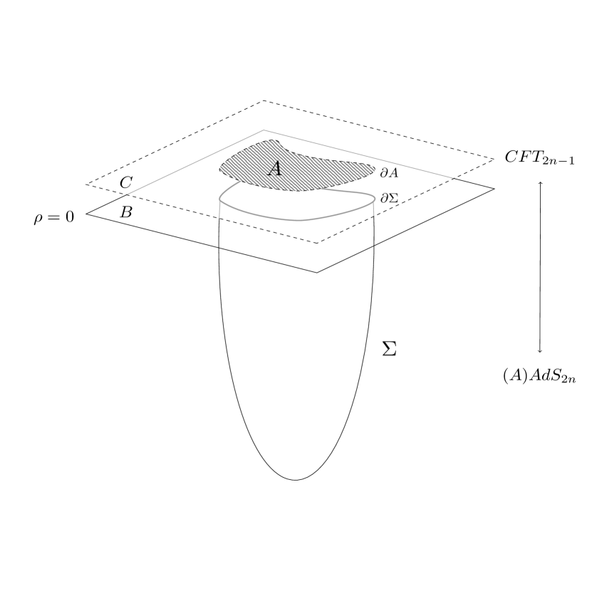
Figure 1: In this diagram, we show all the submanifolds involved in the RT construction. On the field theory side, $C$ is the conformal boundary where the CFT is defined, $A$ is the entangling region and $\partial A$ is the entangling surface. On the gravity side, $B$ is the boundary of spacetime, $\Sigma$ is the minimal surface in the bulk and $\partial\Sigma$ is its border at the spacetime boundary. Both sides are related such that $C$ is conformal to $B$ and $\partial A$ is conformal to $\partial\Sigma$.

As it is well known, the RT proposal for the EE is divergent due to the presence of an infinite conformal factor at the boundary $B$. This is apparent in the Fefferman-Graham (FG) expansion of the AAdS metric FeffermanGraham ; Imbimbo . There are different methods for renormalizing the EE. For example, the scheme proposed by Taylor and Woodhead Marika , which is based on the standard Holographic Renormalization procedure UsualCounterJohnson ; DirichletKraus(quasiloc) ; DirichletHSS(quasiloc) ; DirichletBalaKraus(quasiloc) ; DirichletHS(ano) ; SkenderisAndPapa1 ; SkenderisAndPapa2 . There is also the alternative topological renormalization scheme proposed in Ref.AAO1 , which is based on the Kounterterms renormalization procedure K1Even ; K2Odd ; K3AdS ; KounterComparison ; KounterComparison2 .

Both renormalization schemes rely on writing the EE in terms of the Euclidean gravitational action in the bulk, including its corresponding counterterms at the boundary $B$. As shown by Lewkowycz and Maldacena Maldacena1 , and by Dong RenyiXiDong , the replica trick can be used to construct a suitable $2n-$dimensional bulk replica orbifold $\widehat{M}_{2n}^{(\alpha)}$, which is a squashed-cone (conically singular manifold without U$\left(1\right)$ isometry) having conical angular parameter $\alpha$, such that $2\pi\left(1-\alpha\right)$ is its angular deficit. Then, using the AdS/CFT correspondence in the semi-classical limit, the EE can be expressed as

$$S_{EE}=\left.-\partial_{\alpha}I_{E}\left[\widehat{M}_{2n}^{(\alpha)}\right]\right|_{\alpha=1},$$ (1)

where $I_{E}$ is the Euclidean gravitational action in the bulk, evaluated on the $\widehat{M}_{2n}^{(\alpha)}$ orbifold. If $I_{E}$ is chosen as the Euclidean Einstein-Hilbert (EH) action, then Eq.(1) reproduces the RT proposal for the EE. However, it is apparent that if $I_{E}$ is chosen instead as a suitably renormalized gravitational action, then $S_{EE}$ will be renormalized as well.

Here, we consider the renormalized Euclidean action $I_{E}^{ren}$ as given by the Kounterterms scheme for even-dimensional manifolds in Ref.K1Even . Then we proceed in the same manner than in Ref.AAO1 , but now considering that the action has to be evaluated on a squashed-cone of higher even dimension (beyond the particular case of $D=4$). After taking the corresponding derivative with respect to the angular parameter, we obtain that the renormalized entanglement entropy $S_{EE}^{ren}$ is given by

$$S_{EE}^{ren}=\frac{Vol\left(\Sigma\right)}{4G}+\frac{\left(-1\right)^{n}\ell^{2\left(n-1\right)}}{4G\left[2\left(n-1\right)\right]!}\int\limits_{\partial\Sigma}B_{2n-3},$$ (2)

where $\ell$ is the AdS radius, $Vol\left(\Sigma\right)$ is the volume of the codimension-2 extremal surface $\Sigma$ and $B_{2n-3}$ is the $\left(n-1\right)-$th Chern form evaluated at $\partial\Sigma$, whose explicit form is given in Eq.(36). The derivation of Eq.(2) and its properties are further explained in section III. The first term of Eq.(2) is exactly the RT proposal. Therefore, the counterterm that renormalizes the EE is given by the $B_{2n-3}$ part, which depends on the induced metric $\widetilde{\gamma}$ on $\partial\Sigma$, and on both the intrinsic curvature of $\partial\Sigma$ and its extrinsic curvature with respect to the radial foliation.

The expression for $S_{EE}^{ren}$ given in Eq.(2) can be rewritten in terms of the Euler characteristic and the AdS curvature OleaF of the minimal surface $\Sigma$, as explained in section III.3. This is done by considering the usual Euler theorem for regular manifolds, which relates the Chern form at $\partial\Sigma$ with the Euler density on $\Sigma$. After some algebraic manipulations, $S_{EE}^{ren}$ can be expressed as

$$S_{EE}^{ren}={\displaystyle\int\limits_{\Sigma}}\frac{d^{2n-2}y\sqrt{\gamma}\ell^{2\left(n-1\right)}}{4G2^{\left(n-1\right)}\left(2n-2\right)!}{\displaystyle\sum\limits_{k=1}^{n-1}}\frac{\left(-1\right)^{\left(1+k\right)}\left[2\left(n-1-k\right)\right]!2^{\left(n-1-k\right)}}{\ell^{2\left(n-1-k\right)}}\binom{n-1}{k}\times$$

$$\times\delta_{\left[a_{1}...a_{2k}\right]}^{\left[b_{1}...b_{2k}\right]}\left(\mathcal{F}_{\left.AdS\right|_{\Sigma}}\right)_{b_{1}b_{2}}^{a_{1}a_{2}}\cdots\left(\mathcal{F}_{\left.AdS\right|_{\Sigma}}\right)_{b_{2k-1}b_{2k}}^{a_{2k-1}a_{2k}}+C_{\chi}\,,$$ (3)

where

$$C_{\chi}=\frac{\left(-1\right)^{n+1}\left(4\pi\right)^{\left(n-1\right)}\left(n-1\right)!\ell^{2\left(n-1\right)}}{4G\left(2n-2\right)!}\chi\left[\Sigma\right]\,,$$

and

$$\left(\mathcal{F}_{\left.AdS\right|_{\Sigma}}\right)_{b_{1}b_{2}}^{a_{1}a_{2}}=\mathcal{R}_{b_{1}b_{2}}^{a_{1}a_{2}}+\frac{1}{\ell^{2}}\delta_{\left[b_{1}b_{2}\right]}^{\left[a_{1}a_{2}\right]}\,,$$ (4)

is the AdS curvature of $\Sigma$, which depends on its intrinsic Riemann curvature tensor, and $\chi\left[\Sigma\right]$ is the Euler characteristic of $\Sigma$. This topological form of $S_{EE}^{ren}$ is useful for computing the renormalized EE of certain entangling regions, which give rise to constant curvature minimal surfaces in the bulk. For example, in section IV, we discuss the case of ball-shaped entangling regions, where the computation of $S_{EE}^{ren}$ is greatly simplified.

The organization of this paper is as follows: In section II, we discuss a possible generalization of the Euler theorem for squashed cones in even dimensions. In section III, we derive $S_{EE}^{ren}$ by introducing the renormalized gravitational action for AAdS_2n evaluated on the replica orbifold. We verify the cancellation of the divergence in $S_{EE}^{ren}$ up to next-to-leading order in the radial coordinate $\rho$. We also reinterpret $S_{EE}^{ren}$ in terms of the topological and geometric properties of $\Sigma$. In section IV, we rederive $S_{EE}^{ren}$ for spherical entangling surfaces in odd-dimensional CFTs by using the topological renormalization scheme of Eq.(3), recovering the results of Refs.NishiokaPaper ; NishiokaReview . We also comment on the simplicity of the computation using the topological scheme. Finally, in section V, we comment on the application of the renormalization procedure for characterizing odd-dimensional CFTs and future generalizations thereof.

II Euler density for even-dimensional squashed cones

In Ref.AAO1 , we discussed the Euler theorem for squashed cones in 4D, which was derived by Fursaev, Patrushev and Solodukhin in Ref.SolodukhinNew considering the form of the quadratic curvature invariants on squashed-cone manifolds, which have non-trivial extrinsic curvature contributions coming from the binormal foliation at the tip of the cone. The theorem states that

$$\int\limits_{M_{4}^{\left(\alpha\right)}}\varepsilon_{4}^{\left(\alpha\right)}=\int\limits_{M_{4}}\varepsilon_{4}^{\left(r\right)}+8\pi\left(1-\alpha\right)\int\limits_{\Sigma}\varepsilon_{2}+O\left(\left(1-\alpha\right)^{2}\right),$$ (5)

where $\varepsilon_{4}^{\left(\alpha\right)}$ is the Euler density evaluated on the 4D squashed-cone manifold $\widehat{M}_{4}^{\left(\alpha\right)}$, $\varepsilon_{4}^{\left(r\right)}$ is the Euler density evaluated on a regular manifold $M_{4}$ given by the $\alpha\rightarrow 1$ limit and $\varepsilon_{2}$ is the Euler density evaluated on the 2D manifold $\Sigma$, which is the codimension-2 surface located at the tip of the cone (defined for integer $\left(\frac{1}{\alpha}\right)$ as the fixed-point set of the $Z_{\left(\frac{1}{\alpha}\right)}$ symmetry). The form of $\varepsilon_{4}$, which is also referred to as the Gauss-Bonnet term, is given in terms of the quadratic curvature invariants by

$$\varepsilon_{4}=\sqrt{G}d^{4}x\left(R_{\nu\sigma\lambda}^{\mu}R_{\mu}^{\nu\sigma\lambda}-4R_{\mu\nu}R^{\mu\nu}+R^{2}\right),$$ (6)

and $\varepsilon_{2}=\mathcal{R}\sqrt{\gamma}d^{2}x$, where the cursive $\mathcal{R}$ denotes the Ricci scalar on $\Sigma$.

Furthermore in Ref.AAO1 , we derived a relation between the second Chern form at the spacetime boundary and the first Chern form at $\partial\Sigma$, given by

$$\int\limits_{\partial\widehat{M}_{4}^{\left(\alpha\right)}}B_{3}^{\left(\alpha\right)}=\int\limits_{\partial M_{4}}B_{3}^{\left(r\right)}+8\pi\left(1-\alpha\right)\int\limits_{\partial\Sigma}B_{1}+O\left(\left(1-\alpha\right)^{2}\right).$$ (7)

In order to obtain this, we considered the usual Euler theorem for regular $2n-$dimensional manifolds $M_{2n}$, which states that

$$\int\limits_{M_{2n}}\varepsilon_{2n}=\left(4\pi\right)^{n}n!\chi\left[M_{2n}\right]+\int\limits_{\partial M_{2n}}B_{2n-1},$$ (8)

where $B_{2n-1}$ is the $n-$th Chern form at the boundary $\partial M_{2n}$ (whose form in Gauss normal coordinates is given in Eq.(17)) and $\chi\left[X\right]$ is the Euler characteristic of the manifold $X$. We also considered the relation satisfied by the Euler characteristic of 4D squashed-cones, given by

$$\chi\left[\widehat{M}_{4}^{\left(\alpha\right)}\right]=\chi\left[M_{4}\right]+\left(1-\alpha\right)\chi\left[\Sigma\right]+O\left(\left(1-\alpha\right)^{2}\right),$$ (9)

and derived by FPS in Ref.SolodukhinNew . Then, Eq.(7) can be obtained by considering $n=1$ and $n=2$ in Eq.(8), replacing the $\varepsilon_{4}$ for the $B_{3}$ and the $\varepsilon_{2}$ for the $B_{1}$ in Eq.(5), and then using Eq.(9) to eliminate the Euler characteristics.

We now conjecture that Eqs.(5,7,9) have generalizations for squashed-cone manifolds of arbitrary even dimensions. Namely, we propose that

$$\int\limits_{\widehat{M}_{2n}^{\left(\alpha\right)}}\varepsilon_{2n}^{\left(\alpha\right)}=\int\limits_{M_{2n}}\varepsilon_{2n}^{\left(r\right)}+4n\pi\left(1-\alpha\right)\int\limits_{\Sigma}\varepsilon_{2\left(n-1\right)}+O\left(\left(1-\alpha\right)^{2}\right),$$ (10)

$$\int\limits_{\partial\widehat{M}_{2n}^{\left(\alpha\right)}}B_{2n-1}^{\left(\alpha\right)}=\int\limits_{\partial M_{2n}}B_{2n-1}^{\left(r\right)}+4n\pi\left(1-\alpha\right)\int\limits_{\partial\Sigma}B_{2n-3}+O\left(\left(1-\alpha\right)^{2}\right)$$ (11)

and

$$\chi\left[\widehat{M}_{2n}^{\left(\alpha\right)}\right]=\chi\left[M_{2n}\right]+\left(1-\alpha\right)\chi\left[\Sigma\right]+O\left(\left(1-\alpha\right)^{2}\right).$$ (12)

In the above relations, the Euler density $\varepsilon_{2n}$ is given by

$$\varepsilon_{2n}=\frac{1}{2^{n}}d^{2n}x\sqrt{G}\delta_{\left[\mu_{1}...\mu_{2n}\right]}^{\left[\nu_{1}...\nu_{2n}\right]}R_{\nu_{1}\nu_{2}}^{\mu_{1}\mu_{2}}...R_{\nu_{2n-1}\nu_{2n}}^{\mu_{2n-1}\mu_{2n}},$$ (13)

$B_{2n-1}^{\left(\alpha\right)}$ is the $n-$th Chern form evaluated at the conically-singular $\partial\widehat{M}_{2n}^{\left(\alpha\right)}$ boundary, $B_{2n-1}^{\left(r\right)}$ is the $n-$th Chern form evaluated at the regular $\partial M_{2n}$ boundary (corresponding to the $\alpha\rightarrow 1$ limit) and $B_{2n-3}$ is the $\left(n-1\right)-$th Chern form evaluated at $\partial\Sigma$. Also, $\delta_{\left[\mu_{1}...\mu_{2n}\right]}^{\left[\nu_{1}...\nu_{2n}\right]}$ is the totally antisymmetric generalization of the Kronecker delta, defined by

$$\delta_{\left[\mu_{1}...\mu_{2n}\right]}^{\left[\nu_{1}...\nu_{2n}\right]}\overset{def}{=}\det\left[\delta_{\mu_{1}}^{\nu_{1}}\cdots\delta_{\mu_{k}}^{\nu_{k}}\right].$$ (14)

We mention that Eqs.(10-12) were proven by Fursaev and Solodukhin in Ref.Solodukhin1 for the case of conically-singular manifolds with a U$\left(1\right)$ rotational isometry about the symmetry axis of the cone. Here we simply assume these equations to hold also for the squashed-cone case, and we show that if they are correct, then the $S_{EE}^{ren}$ for arbitrary odd-dimensional holographic CFTs can be obtained in a manner analogous to the 3D case studied in Ref.AAO1 . Conversely, as we will explicitly verify (up to next-to-leading order in the holographic radial coordinate $\rho$) in section III.2, the $S_{EE}^{ren}$ obtained in this manner does indeed renormalize the EE, which lends credence to our conjectured generalization of the Euler theorem, although it does not constitute a proof thereof.

The expression given in Eq.(11) is precisely what is used in section III in order to evaluate the Euclidean action in the replica orbifold, as required in the computation of $S_{EE}$ according to Eq.(1). This ultimately gives the expression for $S_{EE}^{ren}$ when considering the renormalized Euclidean action for AAdS_2n, which is discussed in the following section.

III Renormalization of EE in AdS_2n/CFT_2n-1 through the Chern form

In this section, we study the renormalization of EE via the topological scheme. We consider the renormalized Euclidean gravity action for AAdS_2n spacetimes given in Ref.K1Even , which was obtained by the Kounterterms procedure K1Even ; K2Odd ; K3AdS ; KounterComparison ; KounterComparison2 . The preference for this renormalization procedure over the usual holographic renormalization scheme is only due to practical reasons, as both schemes have been shown to give assymptotically equivalent results for the renormalized action KounterComparison ; KounterComparison2 . Essentially, as explained in Ref.AAO1 , the renormalization of the even-dimensional action in the Kounterterms scheme can be accomplished by the addition of the Chern form (with a specific coupling), which constitutes a single boundary counterterm, whereas in the case of holographic renormalization, the number of required counterterms rapidly grows with the dimension.

The renormalized bulk action, when evaluated in the replica orbifold (as described in the introduction), is given by

$$I_{E}^{ren}=\frac{1}{16\pi G}{\displaystyle\int\limits_{\hat{M}_{2n}^{\left(\alpha\right)}}}d^{2n}x\sqrt{G}\left(R^{\left(\alpha\right)}-2\Lambda\right)+\frac{c_{2n}}{16\pi G}{\displaystyle\int\limits_{\partial\hat{M}_{2n}^{\left(\alpha\right)}}}B_{2n-1}^{\left(\alpha\right)},$$ (15)

where

$$\Lambda=-\frac{\left(2n-1\right)\left(2n-2\right)}{2\ell^{2}},$$

     (16)

and the $n-$th Chern form $B_{2n-1}$ is given by

$$B_{2n-1}=-2n{\displaystyle\int\limits_{0}^{1}}dtd^{2n-1}x\sqrt{h}\delta_{[i_{1}...i_{2n-1}]}^{[j_{1}...j_{2n-1}]}K_{j_{1}}^{i_{1}}\left(\frac{1}{2}\mathcal{R}_{j_{2}j_{3}}^{i_{2}i_{3}}-t^{2}K_{j_{2}}^{i_{2}}K_{j_{3}}^{i_{3}}\right)\times\ldots$$

$$\ldots\times\left(\frac{1}{2}\mathcal{R}_{j_{2n-2}j_{2n-1}}^{i_{2n-2}i_{2n-1}}-t^{2}K_{j_{2n-2}}^{i_{2n-2}}K_{j_{2n-1}}^{i_{2n-1}}\right)\,.$$ (17)

In the expression for the Chern form of Eq.(17), $h_{ij}$ is the metric at the spacetime boundary $B$, $\mathcal{R}_{ij}^{k\ell}$ is the intrinsic Riemann tensor computed with $h_{ij}$, and $K_{j}^{i}$ is the extrinsic curvature of $B$ with respect to the radial foliation. Also, we note that in Eq.(15), $B_{2n-1}^{\left(\alpha\right)}$ denotes the Chern form evaluated at the conically singular boundary of the $\hat{M}_{2n}^{\left(\alpha\right)}$ orbifold, which can be expressed in terms of the Chern form at the boundary of the minimal surface $\Sigma$ using our conjectured generalization of the Euler theorem to squashed-cones in arbitrary even dimensions, as presented in Eq.(11).

When computing the EE, after taking the $\alpha$ derivative according to Eq.(1), the Einstein-Hilbert part simply gives the usual RT minimal area prescription for the EE, as shown by Lewkowicz and Maldacena Maldacena1 and by Dong RenyiXiDong . The EE counterterm then comes from the term containing the boundary Chern form $B_{2n-1}^{\left(\alpha\right)}$. We therefore define the counterterm of the Euclidean action as

$$I_{E}^{ct}=\frac{c_{2n}}{16\pi G}{\displaystyle\int\limits_{\partial\hat{M}_{2n}^{\left(\alpha\right)}}}B_{2n-1}^{\left(\alpha\right)},$$ (18)

and we proceed to compute the counterterm of the EE ($S_{EE}^{ct}$) as

$$S_{EE}^{ct}=\left.-\partial_{\alpha}I_{E}^{ct}\left(\partial\widehat{M}_{2n}^{(\alpha)}\right)\right|_{\alpha=1},$$ (19)

such that $S_{EE}^{ren}=S_{EE}^{RT}+S_{EE}^{ct}$, where $S_{EE}^{RT}$ is the usual RT prescription for the EE. Finally, using Eq.(11) to evaluate $I_{E}^{ct}$, we obtain

$$S_{EE}^{ct}=\frac{\left(-1\right)^{n}\ell^{2\left(n-1\right)}}{4G\left[2\left(n-1\right)\right]!}\int\limits_{\partial\Sigma}B_{2n-3},$$ (20)

recovering $S_{EE}^{ren}$ as given in Eq.(2).

III.1 Explicit covariant embedding

Now, we consider the embedding of the minimal surface $\Sigma$ in the AAdS bulk as given by Hung, Myers and Smolkin HungMyersSmolkin , and by Schwimmer and Theisen SchwimmerAndTheisen . The embedding is such that the bulk coordinates $\left\{\rho,x^{i}\right\}$ of $\Sigma$ and its worldvolume coordinates $\left\{\tau,y^{a}\right\}$ are related by

$$x^{i}\left(\tau,y^{a}\right)=\left(x^{\left(0\right)}\right)^{i}\left(y^{a}\right)+\tau\left(x^{\left(2\right)}\right)^{i}\left(y^{a}\right)+...$$

       (21)

We also consider the asymptotic expansion of the bulk metric $G_{\mu\nu}$, which is of FG form FeffermanGraham and is given by

$$ds_{G}^{2}=G_{\mu\nu}dx^{\mu}dx^{\nu}=\frac{\ell^{2}d\rho^{2}}{4\rho^{2}}+h_{ij}\left(\rho,x\right)dx^{i}dx^{j},$$

           (22)

as presented in Ref.Imbimbo . Here, $\rho$ is the holographic radial coordinate and $h_{ij}$ is the induced metric at the spacetime boundary $B$, which is located at $\rho=0$.

We now consider the induced metric $\gamma_{ab}$ at the minimal surface $\Sigma$, which is defined as the pullback of $G_{\mu\nu}$ in the FG gauge, and is therefore given by

$$\gamma_{ab}=\frac{\partial x^{\mu}}{\partial y^{a}}\frac{\partial x^{\nu}}{\partial y^{b}}G_{\mu\nu}.$$ (23)

Fixing the diffeomorphism gauge as $\tau=\rho$ and $\gamma_{a\tau}=0$, we obtain a FG-like expansion for $\gamma_{ab}$ such that

$$ds_{\gamma}^{2}=\gamma_{ab}dy^{a}dy^{b}=\frac{\ell^{2}}{4\tau^{2}}\left(1+\frac{\tau\ell^{2}}{\left(d-2\right)^{2}}\kappa^{i}\kappa^{j}g_{ij}^{\left(0\right)}+...\right)d\tau^{2}+\widetilde{\gamma}_{ab}\left(\tau,y\right)dy^{a}dy^{b},$$

           (24)

In the previous expansions, $d$ is defined as the dimension of the spacetime boundary ($d=2n-1$). Also, $g_{ij}^{\left(0\right)}$ corresponds to the metric of the CFT at the conformal boundary $C$ (conformal to $B$) and $\sigma_{ab}^{\left(0\right)}$ denotes the induced metric on the entangling surface $\partial A$ (conformal to $\partial\Sigma$) which is given by

$$\sigma_{ab}^{\left(0\right)}=\frac{\partial\left(x^{\left(0\right)}\right)^{i}}{\partial y^{a}}\frac{\partial\left(x^{\left(0\right)}\right)^{j}}{\partial y^{b}}g_{ij}^{\left(0\right)}.$$ (25)

Moreover, $g_{ij}^{\left(2\right)}=-\ell^{2}S_{ij}^{\left(0\right)}$ where $S_{ij}^{\left(0\right)}$, defined as

$$\left(S^{\left(0\right)}\right)_{ij}=\frac{1}{\left(2n-3\right)}\left(R_{ij}^{\left(0\right)}-\frac{g_{ij}^{\left(0\right)}}{2\left(2n-2\right)}R^{\left(0\right)}\right),$$ (26)

denotes the Schouten tensor of the $g_{ij}^{\left(0\right)}$. Now, considering the definition of $\gamma_{ab}$ given in Eq.(23) and the embedding of $\Sigma$ from Eq.(21), we obtain that

$$\sigma_{ab}^{\left(2\right)}=\frac{\partial\left(x^{\left(0\right)}\right)^{i}}{\partial y^{a}}\frac{\partial\left(x^{\left(0\right)}\right)^{j}}{\partial y^{b}}g_{ij}^{\left(2\right)}-\frac{\ell^{2}}{\left(2n-3\right)}\kappa^{i}\kappa_{ab}^{j}\left(g^{\left(0\right)}\right)_{ij}.$$ (27)

Here,

$$\kappa^{i}=\hat{n}_{\left(n\right)}^{i}\kappa_{ab}^{\left(n\right)}\left(\sigma^{\left(0\right)}\right)^{ab},$$ (28)

such that $\hat{n}_{\left(n\right)}^{i}$ are the orthonormal vectors to $\partial A$ at the conformal boundary $C$ ($n=1,2$), and $\kappa_{ab}^{\left(n\right)}$ are the corresponding extrinsic curvatures of $\partial A$.

In the following subsection, given the explicit embedding of $\Sigma$ in $\widehat{M}_{2n}^{(\alpha)}$ and the corresponding FG expansions of $G_{\mu\nu}$ and $\gamma_{ab}$, we proceed to verify the finiteness of $S_{EE}^{ren}$, as given in Eq.(2).

III.2 Proof of finiteness of S${}_{EE}^{ren}$

We now use the previously discussed embedding of $\Sigma$ in order to verify that $S_{EE}^{ren}$, as defined in Eq.(2), is free from divergences. In order to do this, we first exhibit the divergence structure of $S_{EE}^{RT}$, and then we check that the divergences are exactly cancelled by the $S_{EE}^{ct}$ defined in Eq.(20), without modifying the finite universal part. We mention that although the value of $S_{EE}^{ren}$ depends on the particular choice of entangling surface $\partial A$, the divergence structure of $S_{EE}^{RT}$ and $S_{EE}^{ct}$ do not.

We start by computing the RT part of the EE, according to the minimal area prescription RT1 ; TakayanagiReview . We have that

$$S_{EE}^{RT}=\frac{1}{4G}\int\limits_{\Sigma}d^{2n-2}y\sqrt{\gamma}=\frac{1}{4G}\int\limits_{\partial\Sigma_{\varepsilon}}d^{2n-3}y{\displaystyle\int\limits_{\varepsilon}^{\rho_{\text{max}}}}d\rho\sqrt{\gamma},$$ (29)

where $\rho_{\text{max}}$ is the maximum value of the holographic radial coordinate on the $\Sigma$ surface, which depends on the choice of entangling surface $\partial A$ in the CFT, and $\varepsilon$ is a cutoff such that the $\varepsilon\rightarrow 0$ limit is to be evaluated at the end. Considering the FG-like expansion of $\gamma_{ab}$ given in Eq.(24), we have that

$$\sqrt{\gamma}=\frac{\ell\sqrt{\sigma^{\left(0\right)}}}{2\rho^{\left(2n-1\right)/2}}\left(1+\rho\left[\frac{\ell^{2}}{2\left(2n-3\right)^{2}}\kappa^{i}\kappa^{j}g_{ij}^{\left(0\right)}+\frac{1}{2}tr[\sigma^{\left(2\right)}]\right]+...\right),$$ (30)

and therefore, by performing the $\rho$ integration, we obtain

$${\displaystyle\int\limits_{\varepsilon}^{\rho_{\text{max}}}}d\rho\sqrt{\gamma}=C_{1}+\frac{\ell\sqrt{\sigma^{\left(0\right)}}}{\left(2n-3\right)\varepsilon^{\left(2n-3\right)/2}}\left(1+\varepsilon\left[\frac{\left(2n-3\right)}{2\left(2n-5\right)}tr[\sigma^{\left(2\right)}]+\frac{\ell^{2}}{2\left(2n-5\right)\left(2n-3\right)}\kappa^{i}\kappa^{j}g_{ij}^{\left(0\right)}\right]+...\right),$$

     (31)

where $C_{1}$ is a finite constant that depends on the value of $\rho_{\text{max}}$. Here we can see that the leading and next-to-leading divergences occur at orders $\varepsilon^{-\frac{\left(2n-3\right)}{2}}$ and $\varepsilon^{-\frac{\left(2n-5\right)}{2}}$respectively, as expected.

Now, we consider the form of $\sigma_{ab}^{\left(2\right)}$, which is the second coefficient in the FG expansion of the induced metric $\widetilde{\gamma}_{ab}$ at $\partial\Sigma$ and it is given in Eq.(27). We therefore have that

$$tr\left[\sigma^{\left(2\right)}\right]=-\ell^{2}S\left[\sigma^{\left(0\right)}\right]-\frac{\ell^{2}}{2\left(2n-3\right)}\kappa^{i}\kappa^{j}g_{ij}^{\left(0\right)},$$ (32)

where $S\left[\sigma^{\left(0\right)}\right]$ is the trace of the Schouten tensor of the induced metric $\sigma_{ab}^{\left(0\right)}$ at $\partial A$. Also, considering the definition of the Schouten tensor, its trace can be related to the Ricci scalar of $\sigma_{ab}^{\left(0\right)}$ as

$$S\left[\sigma^{\left(0\right)}\right]=\frac{\mathcal{R}^{\left(0\right)}}{2\left(2n-4\right)}.$$ (33)

Finally, we obtain

$$tr\left[\sigma^{\left(2\right)}\right]=-\ell^{2}\left(\frac{\mathcal{R}^{\left(0\right)}}{2\left(2n-4\right)}+\frac{\kappa^{i}\kappa^{j}g_{ij}^{\left(0\right)}}{2\left(2n-3\right)}\right).$$ (34)

By replacing Eq.(34) into the radial integral of Eq.(31), and after some simplifications, we can rewrite $S_{EE}^{RT}$ as

$$S_{EE}^{RT}=\frac{C_{2}}{4G}+\frac{1}{4G}{\displaystyle\int\limits_{\partial\Sigma_{\varepsilon}}}d^{2n-3}y\frac{\ell\sqrt{\sigma^{\left(0\right)}}}{\left(2n-3\right)\varepsilon^{\left(2n-3\right)/2}}-$$

       (35)

where $\frac{C_{2}}{4G}$ is the finite part of the EE, which depends on the choice of $\partial A$.

We now analyze the asymptotic behavior of the EE counterterm, according to Eq.(20). We have that

$$B_{2n-3}=-2\left(n-1\right){\displaystyle\int\limits_{0}^{1}}dtd^{2n-3}y\sqrt{\widetilde{\gamma}}\delta_{[b_{1}...b_{2n-3}]}^{[a_{1}...a_{2n-3}]}k_{b_{1}}^{a_{1}}\left(\frac{1}{2}\mathcal{R}_{b_{2}b_{3}}^{a_{2}a_{3}}-t^{2}k_{b_{2}}^{a_{2}}k_{b_{3}}^{a_{3}}\right)\times\ldots$$

$$\ldots\times\left(\frac{1}{2}\mathcal{R}_{b_{2n-4}b_{2n-3}}^{a_{2n-4}a_{2n-3}}-t^{2}k_{b_{2n-4}}^{a_{2n-4}}k_{b_{2n-3}}^{a_{2n-3}}\right)\,,$$ (36)

where $\mathcal{R}_{b_{1}b_{2}}^{a_{1}a_{2}}$ is the Riemann tensor of the $\widetilde{\gamma}$ metric at $\partial\Sigma$, $k_{b}^{a}=\widetilde{\gamma}^{ac}k_{cb}$ and $k_{cb}$ is the extrinsic curvature of $\partial\Sigma$ with respect to the radial foliation along the holographic coordinate $\rho$ (not to be confused with $\kappa_{ab}^{\left(n\right)}$ for $\partial A$ or with $K_{ij}$ for $B$). By definition,

$$k_{ab}=\frac{-1}{2\sqrt{\gamma_{\rho\rho}}}\partial_{\rho}\widetilde{\gamma}_{ab},$$ (37)

and therefore, using the FG expansion for $\gamma_{ab}$ given in Eq.(24) and considering that

$$\widetilde{\gamma}^{ab}=\rho\left(\left(\sigma^{\left(0\right)}\right)^{ab}-\rho\left(\sigma^{\left(2\right)}\right)^{ab}\right),$$ (38)

we have that

$$k_{b}^{a}=\frac{1}{\ell}\left(\delta_{b}^{a}-\rho\left[\left(\sigma^{\left(2\right)}\right)_{b}^{a}+\frac{\ell^{2}\kappa^{i}\kappa^{j}g_{ij}^{\left(0\right)}}{2\left(2n-3\right)^{2}}\delta_{b}^{a}\right]+...\right).$$ (39)

We also have that $\sqrt{\widetilde{\gamma}}$ is given by

$$\sqrt{\widetilde{\gamma}}=\frac{\sqrt{\sigma^{\left(0\right)}}}{\rho^{\left(2n-3\right)/2}}\left(1+\frac{\rho}{2}tr[\sigma^{\left(2\right)}]+...\right),$$ (40)

and that the Riemann tensor of $\widetilde{\gamma}_{ab}$ satisfies

$$\mathcal{R}_{b_{1}b_{2}}^{a_{1}a_{2}}=\left(\rho\left(\mathcal{R}^{\left(0\right)}\right)_{b_{1}b_{2}}^{a_{1}a_{2}}+...\right),$$ (41)

where $\left(\mathcal{R}^{\left(0\right)}\right)_{b_{1}b_{2}}^{a_{1}a_{2}}$ is the Riemann tensor of the $\sigma_{ab}^{\left(0\right)}$ metric. We now have everything we need in order to expand $B_{2n-3}$ to next-to-leading order in $\rho$. The explicit step-by-step computation is presented in appendix A.

We therefore obtain that the $\left(n-1\right)-$th Chern form at $\partial\Sigma$, located at $\rho=\varepsilon$, is given by

$$B_{2n-3} =\frac{2\left(n-1\right)\left(-1\right)^{\left(n-1\right)}\left[2\left(n-2\right)\right]!}{\ell^{\left(2n-3\right)}}\frac{d^{2n-3}y\sqrt{\sigma_{\alpha\beta}^{\left(0\right)}}}{\varepsilon^{\left(2n-3\right)/2}}\left\{1-\frac{\varepsilon}{2\left(2n-3\right)\left(2n-5\right)}\times\right.$$

$$\times\left.\left[\left(2n-3\right)\left(2n-5\right)tr[\sigma^{\left(2\right)}]+\left(2n-5\right)\kappa^{i}\kappa^{j}g_{ij}^{\left(0\right)}\ell^{2}+\left(2n-3\right)\ell^{2}\mathcal{R}^{\left(0\right)}\right]+\cdots\right\}\,,$$ (42)

and thus, $S_{EE}^{ct}$ is given by

$$S_{EE}^{ct}=-\frac{\ell}{4G\left(2n-3\right)}{\displaystyle\int\limits_{\partial\Sigma_{\varepsilon}}}d^{2n-3}y\frac{\sqrt{\sigma_{\alpha\beta}^{\left(0\right)}}}{\varepsilon^{\left(2n-3\right)/2}}\left\{1-\frac{\varepsilon}{2\left(2n-3\right)\left(2n-5\right)}\left[\left(2n-3\right)\left(2n-5\right)tr[\sigma^{\left(2\right)}]+\right.\right.$$

$$+\left.\left.\left(2n-5\right)\kappa^{i}\kappa^{j}g_{ij}^{\left(0\right)}\ell^{2}+\left(2n-3\right)\ell^{2}\mathcal{R}^{\left(0\right)}\right]+\cdots\right\}\,.$$ (43)

Finally, using Eq.(34), we can rewrite $S_{EE}^{ct}$ as

$$S_{EE}^{ct}=-\frac{1}{4G}{\displaystyle\int\limits_{\partial\Sigma_{\varepsilon}}}d^{2n-3}y\frac{\ell\sqrt{\sigma^{\left(0\right)}}}{\left(2n-3\right)\varepsilon^{\left(2n-3\right)/2}}+$$

         (44)

which explicitly cancells the divergences of $S_{EE}^{RT}$ as presented in Eq.(35), up to next-to-leading order in $\rho=\varepsilon$.

By considering the definition of $S_{EE}^{ren}$, given as the sum of $S_{EE}^{RT}$ and $S_{EE}^{ct}$, and by using Eq.(35) and Eq.(44), we finally obtain that $S_{EE}^{ren}=\frac{C_{2}}{4G}$, where $C_{2}$ is $O\left(1\right)$. Therefore, we have explicitly verified, up to next-to-leading order, that the definition of renormalized EE as given in Eq.(2) is correct, being finite and equal to the universal part or the EE. Furthermore, we consider the explicitly verified cancellation of divergences as evidence of the validity of the generalization of the Euler theorem to squashed cones of arbitrary even dimensions, which to the best of our knowledge, has no formal proof yet.

Finally, we note that the EE counterterms can be rewritten in purely intrinsic form, in terms of the induced metric $\widetilde{\gamma}$ and its curvature invariants, up to linear order in the curvature. To achieve this, we first invert the FG expansion of $\sqrt{\widetilde{\gamma}}$, starting from Eq.(40), to obtain that

$$\sqrt{\sigma^{\left(0\right)}}=\varepsilon^{\frac{2n-3}{2}}\sqrt{\widetilde{\gamma}}\left(1-\frac{1}{2}\varepsilon tr\left[\sigma^{\left(2\right)}\right]+...\right)=\varepsilon^{\frac{2n-3}{2}}\sqrt{\widetilde{\gamma}}-\frac{1}{2}\varepsilon^{\frac{2n-1}{2}}\sqrt{\widetilde{\gamma}}tr\left[\sigma^{\left(2\right)}\right]+...$$ (45)

Then, we replace this into Eq.(44), and after some simplifications, which include substituting for $tr\left[\sigma^{\left(2\right)}\right]$ using Eq.(34), and relating the Ricci scalars of $\widetilde{\gamma}_{ab}$ and $\sigma_{ab}^{\left(0\right)}$ using Eq.(41), we have that up to order $\varepsilon^{-\left(2n-5\right)/2}$, $S_{EE}^{ct}$ is given by

$$S_{EE}^{ct}=-\frac{1}{4G}{\displaystyle\int\limits_{\partial\Sigma_{\varepsilon}}}d^{2n-3}y\frac{\ell\sqrt{\widetilde{\gamma}}}{\left(2n-3\right)}+\frac{1}{4G}{\displaystyle\int\limits_{\partial\Sigma_{\varepsilon}}}d^{2n-3}y\frac{\ell^{3}\sqrt{\widetilde{\gamma}}}{2\left(2n-3\right)\left(2n-4\right)\left(2n-5\right)}\mathcal{R}\left[\widetilde{\gamma}_{ab}\right]+...,$$

                 (46)

which is written in terms of purely intrinsic quantities. This intrinsic form of the counterterms allows to make contact with the EE renormalization scheme presented in Ref.Marika . In appendix B, we show how it can be derived starting directly from $S_{EE}^{ct}$ written in terms of the Chern form, as given in Eq.(20).

III.3 Topological interpretation of renormalized EE for the AdS_2n/CFT_2n-1 case

We now reinterpret $S_{EE}^{ren}$ as given in Eq.(2), in terms of the topological and geometric properties of the minimal surface $\Sigma$ as an AAdS submanifold. In particular, we rewrite $S_{EE}^{ren}$ in terms of the Euler characteristic of $\Sigma$ and its AdS curvature OleaF .

By considering the Euler theorem, as presented in Eq.(8), we have that the Chern form which gives the EE counterterm can be rewritten as

$${\displaystyle\int\limits_{\partial\Sigma}}B_{2n-3}={\displaystyle\int\limits_{\Sigma}}d^{2n-2}y\sqrt{\gamma}\varepsilon_{2n-2}-\left(4\pi\right)^{\left(n-1\right)}\left(n-1\right)!\chi\left[\Sigma\right],$$ (47)

where $\varepsilon_{2n-2}$ is the Euler density of $\Sigma$ and $\chi\left[\Sigma\right]$ is its Euler characteristic. Then, $S_{EE}^{ren}$ can be expressed as

$$S_{EE}^{ren}=\frac{1}{4G}\left({\displaystyle\int\limits_{\Sigma}}d^{2n-2}y\sqrt{\gamma}+\frac{\left(-1\right)^{n}\ell^{2\left(n-1\right)}}{\left(2n-2\right)!}{\displaystyle\int\limits_{\Sigma}}d^{2n-2}y\sqrt{\gamma}\varepsilon_{2n-2}\right)+$$

$$+\frac{\left(-1\right)^{n+1}\left(4\pi\right)^{\left(n-1\right)}\left(n-1\right)!\ell^{2\left(n-1\right)}}{4G\left(2n-2\right)!}\chi\left[\Sigma\right]\,.$$ (48)

We now define the topological constant $C_{\chi}$ as

$$C_{\chi}=\frac{\left(-1\right)^{n+1}\left(4\pi\right)^{\left(n-1\right)}\left(n-1\right)!\ell^{2\left(n-1\right)}}{4G\left(2n-2\right)!}\chi\left[\Sigma\right],$$ (49)

and using the definition of $\varepsilon_{2n-2}$ given in Eq.(13), we can write $S_{EE}^{ren}$ as

$$S_{EE}^{ren}=\frac{1}{4G}{\displaystyle\int\limits_{\Sigma}}d^{2n-2}y\sqrt{\gamma}\left(1+\frac{\left(-1\right)^{n}\ell^{2\left(n-1\right)}}{\left(2n-2\right)!2^{\left(n-1\right)}}\delta_{\left[a_{1}...a_{2n-2}\right]}^{\left[b_{1}...b_{2n-2}\right]}\mathcal{R}_{b_{1}b_{2}}^{a_{1}a_{2}}...\mathcal{R}_{b_{2n-3}b_{2n-2}}^{a_{2n-3}a_{2n-2}}\right)+C_{\chi}\,,$$ (50)

where $\mathcal{R}_{b_{1}b_{2}}^{a_{1}a_{2}}$ is the Riemann tensor of the induced metric $\gamma_{ab}$ on $\Sigma$. Finally, we can simplify Eq.(50) by considering the properties of the antisymmetric Kronecker delta. In particular, we have that

$$S_{EE}^{ren}=\frac{\ell^{2\left(n-1\right)}}{4G2^{\left(n-1\right)}\left(2n-2\right)!}{\displaystyle\int\limits_{\Sigma}}d^{2n-2}y\sqrt{\gamma}\delta_{\left[a_{1}...a_{2n-2}\right]}^{\left[b_{1}...b_{2n-2}\right]}\left[\left(-1\right)^{n}\mathcal{R}_{b_{1}b_{2}}^{a_{1}a_{2}}...\mathcal{R}_{b_{2n-3}b_{2n-2}}^{a_{2n-3}a_{2n-2}}+\right.$$

$$+\left.\frac{1}{\ell^{2\left(n-1\right)}}\delta_{\left[b_{1}b_{2}\right]}^{\left[a_{1}a_{2}\right]}...\delta_{\left[b_{2n-3}b_{2n-2}\right]}^{\left[a_{2n-3}a_{2n-2}\right]}\right]+C_{\chi}\,.$$ (51)

Now, we express $S_{EE}^{ren}$ in terms of the AdS curvature $\mathcal{F}_{AdS}$, which for a general AAdS manifold is defined as

$$\left(\mathcal{F}_{AdS}\right)_{\nu_{1}\nu_{2}}^{\mu_{1}\mu_{2}}=R_{\nu_{1}\nu_{2}}^{\mu_{1}\mu_{2}}+\frac{1}{\ell^{2}}\delta_{\left[\nu_{1}\nu_{2}\right]}^{\left[\mu_{1}\mu_{2}\right]},$$ (52)

where $R_{\nu_{1}\nu_{2}}^{\mu_{1}\mu_{2}}$ is the Riemann tensor of the manifold. Then, for the $\Sigma$ manifold, the product of the Riemann tensors can be reexpressed in terms of the AdS curvature as

$$\mathcal{R}_{b_{1}b_{2}}^{a_{1}a_{2}}...\mathcal{R}_{b_{2n-3}b_{2n-2}}^{a_{2n-3}a_{2n-2}}=\left(\left(\mathcal{F}_{\left.AdS\right|_{\Sigma}}\right)_{b_{1}b_{2}}^{a_{1}a_{2}}-\frac{1}{\ell^{2}}\delta_{\left[b_{1}b_{2}\right]}^{\left[a_{1}a_{2}\right]}\right)\cdots\left(\left(\mathcal{F}_{\left.AdS\right|_{\Sigma}}\right)_{b_{2n-3}b_{2n-2}}^{a_{2n-3}a_{2n-2}}-\frac{1}{\ell^{2}}\delta_{\left[b_{2n-3}b_{2n-2}\right]}^{\left[a_{2n-3}a_{2n-2}\right]}\right)$$

(53)

where we have disregarded the order of the indices due to the presence of the overall Kronecker delta. Now, noting that the $k=0$ term cancells the deltas appearing in Eq.(51), we can write

$$S_{EE}^{ren}={\displaystyle\int\limits_{\Sigma}}\frac{d^{2n-2}y\sqrt{\gamma}\ell^{2\left(n-1\right)}}{4G2^{\left(n-1\right)}\left(2n-2\right)!}\delta_{\left[a_{1}...a_{2n-2}\right]}^{\left[b_{1}...b_{2n-2}\right]}{\displaystyle\sum\limits_{k=1}^{n-1}}\frac{\left(-1\right)^{1+k}}{\ell^{2\left(n-1-k\right)}}\binom{n-1}{k}\left(\mathcal{F}_{\left.AdS\right|_{\Sigma}}\right)_{b_{1}b_{2}}^{a_{1}a_{2}}\ldots\left(\mathcal{F}_{\left.AdS\right|_{\Sigma}}\right)_{b_{2k-1}b_{2k}}^{a_{2k-1}a_{2k}}\times$$

$$\times\delta_{\left[b_{2k+1}b_{2k+2}\right]}^{\left[a_{2k+1}a_{2k+2}\right]}\ldots\delta_{\left[b_{2n-3}b_{2n-2}\right]}^{\left[a_{2n-3}a_{2n-2}\right]}+C_{\chi}\,.$$ (54)

Finally, using the properties of the antisymmetric delta, we obtain that

$$S_{EE}^{ren}={\displaystyle\int\limits_{\Sigma}}\frac{d^{2n-2}y\sqrt{\gamma}\ell^{2\left(n-1\right)}}{4G2^{\left(n-1\right)}\left(2n-2\right)!}{\displaystyle\sum\limits_{k=1}^{n-1}}\frac{\left(-1\right)^{\left(1+k\right)}\left[2\left(n-1-k\right)\right]!2^{\left(n-1-k\right)}}{\ell^{2\left(n-1-k\right)}}\binom{n-1}{k}\times$$

$$\times\delta_{\left[a_{1}...a_{2k}\right]}^{\left[b_{1}...b_{2k}\right]}\left(\mathcal{F}_{\left.AdS\right|_{\Sigma}}\right)_{b_{1}b_{2}}^{a_{1}a_{2}}\ldots\left(\mathcal{F}_{\left.AdS\right|_{\Sigma}}\right)_{b_{2k-1}b_{2k}}^{a_{2k-1}a_{2k}}+C_{\chi}\,,$$ (55)

where $S_{EE}^{ren}$ has been expressed in terms of contractions of the AdS curvature of $\Sigma$ ($\mathcal{F}_{\left.AdS\right|_{\Sigma}}$) and its Euler characteristic, as considered in the definition of $C_{\chi}$ given in Eq.(49).

We note that Eq.(55) gives an interpretation of renormalized EE in terms of the topological and geometric properties of $\Sigma$ as an AAdS Riemannian manifold, which generalizes the result obtained in Ref.AAO1 for the case of AdS₄/CFT₃.

IV Explicit example: Ball-shaped entangling region in CFT_2n-1, with a global AdS_2n bulk

In order to exhibit the advantages of the topological renormalization scheme, we now rederive the renormalized EE of a ball-shaped entangling region in the ground state of an holographic $\left(2n-1\right)-$dimensional CFT, having global AdS_2n as its gravity dual. This computation was firstly done by Kawano, Nakaguchi and Nishioka in Ref.NishiokaPaper , by evaluating the RT area functional. Instead, we make use of the topological form for $S_{EE}^{ren}$ given in Eq.(55).

We consider that the entangling region is delimited by a spherical entangling surface, such that $\partial A=S^{2n-3}$. Also, the metric $G_{\mu\nu}$ of global AdS_2n can be written as

$$ds_{G}^{2}=\frac{\ell^{2}d\rho^{2}}{4\rho^{2}}+\frac{1}{\rho}\left(-dt^{2}+dr^{2}+r^{2}d\Omega_{2n-3}^{2}\right)=G_{\mu\nu}dx^{\mu}dx^{\nu},$$

   (56)

where the boundary metric has been expressed in spherical coordinates. Now, as shown in appendix C, the minimal surface $\Sigma$ corresponding to the entangling surface $\partial A=S^{2n-3}$ can be parametrized as

$$\Sigma:\left\{t=const~{};~{}r^{2}+\ell^{2}\rho=R^{2}\right\},$$ (57)

where $R$ is the radius of the sphere. We proceed to compute the induced metric $\gamma_{ab}$ on $\Sigma$, defined in Eq.(23), considering that its worldvoume coordinates are given by $y^{a}=\left\{\rho,\theta_{1},...,\theta_{2n-3}\right\}$, whereas the bulk coordinates are $x^{\mu}=\left\{\rho,t,r,\theta_{1},...,\theta_{2n-3}\right\}$. In particular, we obtain that

$$ds_{\gamma}^{2}=\frac{\ell^{2}}{4\rho^{2}}\left(1+\frac{\ell^{2}\rho}{\left(R^{2}-\ell^{2}\rho\right)}\right)d\rho^{2}+\frac{\left(R^{2}-\ell^{2}\rho\right)}{\rho}d\Omega_{2n-3}^{2}=\gamma_{ab}dy^{a}dy^{b}.$$ (58)

Considering the induced metric, we now compute $S_{EE}^{ren}$ using the topological procedure. Given the induced metric of Eq.(58), we compute the AdS curvature on $\Sigma$, according to Eq.(52), and we find that it vanishes identically (i.e., $\left(\mathcal{F}_{\left.AdS\right|_{\Sigma}}\right)_{b_{1}b_{2}}^{a_{1}a_{2}}=0$). Also, we consider that $\Sigma$ is topologically equivalent to a $\left(2n-2\right)-$ball, whose Euler characteristic is $\chi\left(\Sigma\right)=1$. Therefore, using $S_{EE}^{ren}$ as given in Eq.(55), we have that

$$S_{EE}^{ren}=\frac{\left(-1\right)^{n+1}\left(4\pi\right)^{\left(n-1\right)}\left(n-1\right)!\ell^{2\left(n-1\right)}}{4G\left(2n-2\right)!},$$ (59)

which agrees with the standard result as given in Refs.NishiokaPaper ; NishiokaReview . We also conclude from this analysis that for spherical entangling surfaces, the minimal surface $\Sigma$ is a constant curvature surface, which has $\mathcal{R}_{b_{1}b_{2}}^{a_{1}a_{2}}=-\frac{1}{\ell^{2}}\delta_{\left[b_{1}b_{2}\right]}^{\left[a_{1}a_{2}\right]}$.

We note that the computation of the renormalized EE using the topological approach of Eq.(55) is performed directly to all orders in $\rho=\varepsilon$. We also mention that, as further explained in section V, the computation of $S_{EE}^{ren}$ for the case with $\partial A=S^{2n-3}$ is important because it is related to the $a-$ charge S-c-Myers ; NishiokaPaper , such that $S_{EE}^{ren}=\left(-1\right)^{n-1}2\pi a_{2n-1}$. The $a-$charge counts the number of degrees of freedom of the CFT and is conjectured to decrease along RG flows between conformal fixed points. Therefore, it can be thought of as a generalization of Zamolodchikov’s c-theorem cTheo .

Using our result for $S_{EE}^{ren}$, we therefore find that

$$a_{2n-1}=\frac{\left(4\pi\right)^{\left(n-2\right)}\left(n-1\right)!\ell^{2\left(n-1\right)}}{2G\left(2n-2\right)!},$$ (60)

in agreement with the known result as given in Refs.NishiokaPaper ; NishiokaReview . As written, the $a-$charge is expressed in terms of the bulk gravity quantities (like the AdS radius $\ell$ and Newton’s constant $G$), but it can be rewritten entirely in terms of the CFT quantities by using the standard dictionary.

V Outlook

We have successfully extended the topological scheme developed in Ref.AAO1 for computing the renormalized EE to holographic CFTs of arbitrary odd dimensions. This procedure considers adding the Chern form to the usual RT area functional, such that the renormalized EE is written as shown in Eq.(2). Alternatively, $S_{EE}^{ren}$ can be written in terms of the Euler characteristic of the minimal surface $\Sigma$ and its AdS curvature, as shown in Eq.(55). The latter form greatly simplifies the computation of $S_{EE}^{ren}$ and is of interest because it exhibits the relation between the EE and the topological and geometric properties of $\Sigma$. We also make contact with the renormalization procedure developed in Ref.Marika , by writing the EE counterterm in terms of the intrinsic quantities on $\partial\Sigma$, as shown in Eq.(46).

The renormalized EE is of interest for the study of holographic renormalization group (RG) flows. As firstly mentioned in Ref.Marika and also discussed in Ref.NishiokaReview , $S_{EE}^{ren}$ for a ball-shaped entangling region in the ground state of a CFT is related to its $a-$charge S-c-Myers , which encodes information about the number of degrees of freedom of the theory and is conjectured to decrease along RG flows between conformal fixed points. It therefore constitutes a generalization of Zamolodchikov’s c-theorem cTheo . In particular, for a $\left(2n-1\right)-$dimensional CFT, $S_{EE}^{ren}=\left(-1\right)^{n-1}2\pi a_{2n-1}$ where $\left(a_{2n-1}\right)_{UV}\geq\left(a_{2n-1}\right)_{IR}$ between any two fixed points. Using our topological renormalization approach (see Eq.(55)), the computation of $S_{EE}^{ren}$ for spherical entangling surfaces becomes nearly trivial, and as discussed in section IV, we recover the known result given in Refs.NishiokaPaper ; NishiokaReview .

As future work, we will also study how to extend the scheme to AAdS manifolds of arbitrary odd dimensions by using the renormalized Euclidean gravitational action discussed in Ref.K2Odd . We expect this analysis to be useful for the study of the conformal anomaly of the corresponding holographic CFTs. We also intend to apply our topological renormalization scheme to obtain the renormalized EE for higher-curvature theories of gravity, specially those of the Lovelock class Lovelock1 ; Lovelock2 , and to renormalize other information-theoretic measures of holographic CFTs, like the Entanglement Renyi Entropies (EREs) RenyiXiDong ; RenyiHeadrick ; RenyiFreeEnergy ; MyersRenyi and the complexity AliComplexity ; Complexity2 ; Complexity3 ; IgnacioReyes .

Appendix A Explicit expansion of the Chern form

We proceed to simplify and expand the $B_{2n-3}$ Chern form, which appears in the expression for $S_{EE}^{ct}$ as given in Eq.(20). In the following expressions we introduce a short-hand notation, such that the antisymmetric Kronecker deltas are indicated only by the number of indices, i.e., $\delta_{[b_{1}...b_{2n-3}]}^{[a_{1}...a_{2n-3}]}$ is denoted by $\delta_{[2n-3]}^{[2n-3]}$. Also, as the final expression is fully contracted, the indices of all tensors are omitted. For example, $k_{b_{1}}^{a_{1}}k_{b_{2}}^{a_{2}}$ is denoted by $k^{2}$, and $\mathcal{R}_{b_{1}b_{2}}^{a_{1}a_{2}}$, which is the Riemann tensor of the metric $\widetilde{\gamma}$, is denoted as $\mathcal{R}ie$. To avoid ambiguity, traces of tensors are explicitly indicated.

In the new notation, the definition of the Chern form at $\partial\Sigma$, is given by

$$B_{2n-3}=-2\left(n-1\right){\displaystyle\int\limits_{0}^{1}}dtd^{2n-3}y\sqrt{\widetilde{\gamma}}\delta_{\left[2n-3\right]}^{\left[2n-3\right]}k\left(\frac{1}{2}\mathcal{R}ie-t^{2}k^{2}\right)^{n-2},$$ (61)

and the FG expansion of the different quantities are given in section III.2. We note that, in every FG expansion, the $"..."$ represents $O\left(\rho^{2}\right)$ terms.

First, we expand the $k^{2}$ terms, were we have that

$$k^{2}=\frac{1}{\ell^{2}}\left(\delta^{2}-2\rho\left[\delta\sigma^{\left(2\right)}+\frac{\ell^{2}\kappa^{i}\kappa^{j}g_{ij}^{\left(0\right)}}{2\left(2n-3\right)^{2}}\delta^{2}\right]+...\right).$$

(62)

Then, we consider that the term in parenthesis can be expanded as

$$\left(\frac{1}{2}\mathcal{R}ie-t^{2}k^{2}\right)=-\frac{t^{2}}{\ell^{2}}\delta^{2}+\rho\left[\frac{1}{2}\left(\mathcal{R}ie^{\left(0\right)}\right)+\frac{2}{l^{2}}t^{2}\left(\delta\sigma^{\left(2\right)}+\frac{\ell^{2}\kappa^{i}\kappa^{j}g_{ij}^{\left(0\right)}}{2\left(2n-3\right)^{2}}\delta^{2}\right)\right]+\ldots\,.$$

Note that $\mathcal{R}ie^{\left(0\right)}$ is the Riemann tensor of the metric $\sigma^{\left(0\right)}$. The product of such terms, to linear order in $\rho$, becomes

$$\left(\frac{1}{2}\mathcal{R}ie-t^{2}k^{2}\right)^{n-2}=\left(-1\right)^{n-2}\frac{t^{2n-4}}{\ell^{2n-4}}\delta^{2n-4}+$$

$$\rho\left(-1\right)^{n-3}\left(n-2\right)\frac{t^{2n-6}}{\ell^{2n-6}}\delta^{2n-6}\left[\frac{1}{2}\left(\mathcal{R}ie^{\left(0\right)}\right)+\frac{2}{\ell^{2}}t^{2}\left(\delta\sigma^{\left(2\right)}+\frac{\ell^{2}\kappa^{i}\kappa^{j}g_{ij}^{\left(0\right)}}{2\left(2n-3\right)^{2}}\delta^{2}\right)\right]+\ldots\,.$$ (63)

Therefore, $\sqrt{\widetilde{\gamma}}k\left(\frac{1}{2}\mathcal{R}ie-t^{2}k^{2}\right)^{n-2}$ can be expanded as

$$\sqrt{\widetilde{\gamma}}k\left(\frac{1}{2}\mathcal{R}ie-t^{2}k^{2}\right)^{n-2}=\frac{\left(-1\right)^{\left(n-2\right)}\sqrt{\sigma_{\alpha\beta}^{\left(0\right)}}}{\ell^{2n-3}\rho^{\left(2n-3\right)/2}}t^{2n-4}\delta^{2n-3}$$

$$-\frac{\left(-1\right)^{\left(n-2\right)}\sqrt{\sigma_{\alpha\beta}^{\left(0\right)}}}{\ell^{2n-3}\rho^{\left(2n-3\right)/2}}t^{2n-4}\rho\left[-\frac{tr[\sigma^{\left(2\right)}]}{2}\delta^{2n-3}+\left(2n-3\right)\delta^{2n-4}\left(\sigma^{\left(2\right)}\right)\right.$$

$$+\left.\frac{\left(n-2\right)\ell^{2}}{2t^{2}}\delta^{2n-5}\left(\mathcal{R}ie^{\left(0\right)}\right)+\frac{\kappa^{i}\kappa^{j}g_{ij}^{\left(0\right)}\ell^{2}}{2\left(2n-3\right)}\delta^{2n-3}\right]+...~{}.$$ (64)

Thus, the t integral of the previous term has a FG expansion given by

$${\displaystyle\int\limits_{0}^{1}}dt\sqrt{\widetilde{\gamma}}k\left(\frac{1}{2}\mathcal{R}ie-t^{2}k^{2}\right)^{n-2}=\frac{\left(-1\right)^{n-2}\sqrt{\sigma_{\alpha\beta}^{\left(0\right)}}}{\ell^{2n-3}\rho^{\left(2n-3\right)/2}}\frac{1}{2n-3}\delta^{2n-3}$$

$$-\frac{\left(-1\right)^{n-2}\sqrt{\sigma_{\alpha\beta}^{\left(0\right)}}}{\ell^{2n-3}\rho^{\left(2n-3\right)/2}}\frac{1}{2n-3}\rho\left[-\frac{tr[\sigma^{\left(2\right)}]}{2}\delta^{2n-3}+\left(2n-3\right)\delta^{2n-4}\sigma^{\left(2\right)}\right.$$

$$+\left.\frac{\left(n-2\right)\left(2n-3\right)\ell^{2}}{2\left(2n-5\right)}\delta^{2n-5}\left(\mathcal{R}ie^{\left(0\right)}\right)+\frac{\kappa^{i}\kappa^{j}g_{ij}^{\left(0\right)}\ell^{2}}{2\left(2n-3\right)}\delta^{2n-3}\right]+\ldots~{}.$$ (65)

Now, using that

$$\delta_{[j_{1}...j_{m}]}^{[i_{1}...i_{m}]}\delta_{i_{1}}^{j_{1}}...\delta_{i_{k}}^{j_{k}}=\frac{\left(N-m+k\right)!}{\left(N-m\right)!}\delta_{\left[j_{k+1}...j_{m}\right]}^{\left[i_{k+1}...i_{m}\right]},$$

(66)

we can finally obtain the contractions of the integrand, such that

$${\displaystyle\int\limits_{0}^{1}}dt\sqrt{\widetilde{\gamma}}\delta_{\left[2n-3\right]}^{\left[2n-3\right]}k\left(\frac{1}{2}\mathcal{R}ie-t^{2}k^{2}\right)^{n-2}=\frac{\left(-1\right)^{n-2}\left(2n-3\right)!\sqrt{\sigma_{\alpha\beta}^{\left(0\right)}}}{\ell^{2n-3}\left(2n-3\right)\rho^{\left(2n-3\right)/2}}$$

$$-\frac{\left(-1\right)^{n-2}\left(2n-3\right)!\sqrt{\sigma_{\alpha\beta}^{\left(0\right)}}}{\ell^{2n-3}\left(2n-3\right)\rho^{\left(2n-3\right)/2}}\frac{\rho}{2\left(2n-3\right)\left(2n-5\right)}\left[\left(2n-3\right)\left(2n-5\right)tr[\sigma^{\left(2\right)}]\right.$$

$$+\left.\left(2n-5\right)\kappa^{i}\kappa^{j}g_{ij}^{\left(0\right)}\ell^{2}+\left(2n-3\right)\ell^{2}\mathcal{R}^{\left(0\right)}\right]+\ldots~{},$$ (67)

where $\mathcal{R}^{\left(0\right)}$ is the Ricci scalar of the $\sigma^{\left(0\right)}$ metric.

Finally, replacing the previous expression into Eq.(61), we obtain that $B_{2n-3}$ is given by

$$B_{2n-3}=\frac{2\left(n-1\right)\left(-1\right)^{n-1}\left(2n-2\right)!}{\ell^{2n-3}}\frac{d^{2n-3}y\sqrt{\sigma_{\alpha\beta}^{\left(0\right)}}}{\varepsilon^{\left(2n-3\right)/2}}\left\{1-\frac{\varepsilon}{2\left(2n-3\right)\left(2n-5\right)}\left[\left(2n-3\right)\left(2n-5\right)tr[\sigma^{\left(2\right)}]\right.\right.$$

$$+\left.\left.\left(2n-5\right)\kappa^{i}\kappa^{j}g_{ij}^{\left(0\right)}\ell^{2}+\left(2n-3\right)\ell^{2}\mathcal{R}^{\left(0\right)}\right]+\ldots\right\}$$ (68)

which corresponds to Eq.(42) of section III.2 of the main text.

Appendix B Intrinsic counterterms directly from the Chern form

In this appendix we emphasize that the intrinsic counterterms for the EE, as presented in Eq.(46), can be directly obtained starting from the Chern form at $\partial\Sigma$. In particular, considering Eq.(20), we have that

$$S_{EE}^{ct}=\frac{\left(-1\right)^{n}\ell^{2\left(n-1\right)}}{4G\left[2\left(n-1\right)\right]!}{\displaystyle\int\limits_{\partial\Sigma}}B_{2n-3},$$

       (69)

where $B_{2n-3}$ is given in Eq.(61). We use the same shorthand notation introduced in appendix A.

Now, the Riemann tensor of the $\widetilde{\gamma}_{ab}$ can be written in terms of the Weyl tensor and the Schouten tensor, such that

$$\mathcal{R}_{b_{1}b_{2}}^{a_{1}a_{2}}=\mathcal{W}_{b_{1}b_{2}}^{a_{1}a_{2}}+\delta_{[b_{1}}^{[a_{1}}\mathcal{S}_{b_{2}]}^{a_{2}]},$$ (70)

where the antisymmetrization does not have a $\frac{1}{4}$ factor. In turn, the Schouten and the Weyl tensors of the metric $\widetilde{\gamma}_{ab}$ at $\partial\Sigma$ can be expressed in terms of those of the $\sigma_{ab}^{\left(0\right)}$ metric at $\partial A$, to first order in $\rho$, as

$$\mathcal{S}_{b}^{a}=\rho\left(S^{\left(0\right)}\right)_{b}^{a}+...~{},$$

(71)

Then, considering the FG expansion of the extrinsic curvature $k_{b}^{a}$ of $\partial\Sigma$ as given in Eq.(39) and using that $d=2n-1$, we have that

$$k_{b}^{a}=\left(k^{\left(0\right)}\right)_{b}^{a}+\rho\left(k^{\left(2\right)}\right)_{b}^{a}+...,$$

(72)

Finally, using that

$$tr\left[\sigma^{\left(2\right)}\right]=-\ell^{2}S\left[\sigma^{\left(0\right)}\right]-\frac{\ell^{2}}{2\left(2n-3\right)}\kappa^{i}\kappa^{j}g_{ij}^{\left(0\right)},$$ (73)

as given in Eq.(32), we have that

$$tr[k^{\left(2\right)}]=\ell S\left[\sigma^{\left(0\right)}\right]=\ell S^{\left(0\right)}.$$ (74)

We proceed to simplify the expression for $B_{2n-3}$. Using the shorthand notation, we have that

$$k^{2}=\left(k^{\left(0\right)}\right)+2\rho k^{\left(0\right)}k^{\left(2\right)}+...,$$

(75)

and also

$$\left(\frac{1}{2}\mathcal{R}ie-t^{2}k^{2}\right)=-t^{2}\left(k^{\left(0\right)}\right)^{2}+\rho\left[\frac{1}{2}W^{\left(0\right)}+2\delta S^{\left(0\right)}-2t^{2}k^{\left(2\right)}k^{\left(0\right)}\right]+...\,.$$

Now, the product of the previous terms can be expanded as

$$\left(\frac{1}{2}\mathcal{R}ie-t^{2}k^{2}\right)^{n-2}=\left(-t^{2}\right)^{\left(n-2\right)}\left(k^{\left(0\right)}\right)^{2n-4}$$

$$+\rho\left(n-2\right)\left(-t^{2}\right)^{\left(n-3\right)}\left(k^{\left(0\right)}\right)^{2n-6}\left[\frac{1}{2}W^{\left(0\right)}+2S^{\left(0\right)}\delta-2t^{2}k^{\left(2\right)}k^{\left(0\right)}\right]+...~{},$$ (76)

and thus

$$k\left(\frac{1}{2}\mathcal{R}ie-t^{2}k^{2}\right)^{n-2}=\left(-1\right)^{n-2}t^{2n-4}\left(k^{\left(0\right)}\right)^{2n-3}$$

$$+\left(-1\right)^{n-2}\rho\left[-\left(2n-4\right)t^{2n-6}\left(k^{\left(0\right)}\right)^{2n-5}\delta S^{\left(0\right)}+\left(2n-3\right)t^{2n-4}\left(k^{\left(0\right)}\right)^{2n-4}k^{\left(2\right)}\right]+...,$$ (77)

where we used the fact that the contractions of the Weyl tensor, after considering the overall Kronecker delta, vanish identically due to its tracelessnes. Now, using that $\left(k^{\left(0\right)}\right)_{b}^{a}=\frac{1}{\ell}\delta_{b}^{a}$, $tr[k^{\left(2\right)}]=\ell tr\left[S^{\left(0\right)}\right]$ and

$$\delta_{[j_{1}...j_{m}]}^{[i_{1}...i_{m}]}\delta_{i_{1}}^{j_{1}}...\delta_{i_{k}}^{j_{k}}=\frac{\left(N-m+k\right)!}{\left(N-m\right)!}\delta_{\left[j_{k+1}...j_{m}\right]}^{\left[i_{k+1}...i_{m}\right]},$$

(78)

we can compute the contractions with the overall Kronecker delta and perform the t integration in order to obtain that

$${\displaystyle\int\limits_{0}^{1}}dt\delta_{[2n-3]}^{[2n-3]}k\left(\frac{1}{2}\mathcal{R}ie-t^{2}k^{2}\right)^{n-2}=$$

$$\frac{\left(2n-3\right)!}{\ell^{2n-3}}\frac{\left(-1\right)^{n-2}}{2n-3}+\rho\frac{\left(-1\right)^{n-2}\left(2n-4\right)!}{\ell^{2n-5}}\left[1-\frac{2n-4}{2n-5}\right]tr\left[S^{\left(0\right)}\right]+...$$

$$=\/\left(-1\right)^{n-2}\left[\frac{\left(2n-4\right)!}{\ell^{2n-3}}-\rho\frac{\left(2n-6\right)!}{2\ell^{2n-5}}\mathcal{R}^{\left(0\right)}\right]+...~{}.$$ (79)

Finally, using that to the leading order $\mathcal{R}\left[\widetilde{\gamma}\right]\simeq\rho\mathcal{R}^{\left(0\right)}$, where $\mathcal{R}\left[\widetilde{\gamma}\right]$ is the Ricci scalar of the metric $\widetilde{\gamma}$ and $\mathcal{R}^{\left(0\right)}$ is that of $\sigma^{\left(0\right)}$, the expression for $S_{EE}^{ct}$ as given in Eq.(69) can be written entirely in terms of the intrinsic quantities that depend on $\widetilde{\gamma}$, such that

$${\displaystyle\frac{\left(-1\right)^{n+1}}{4G}\frac{\ell^{2n-2}}{\left(2n-3\right)!}\int\limits_{0}^{1}}dt\delta_{[2n-3]}^{[2n-3]}k\left(\frac{1}{2}\mathcal{R}ie-t^{2}k^{2}\right)^{n-2}=$$

$$-\frac{\ell}{4G\left(2n-3\right)}+\frac{\ell^{3}R\left[\widetilde{\gamma}\right]}{4G2(2n-3)\left(2n-4\right)\left(2n-5\right)}+...$$ (80)

and therefore, we obtain

$$S_{EE}^{ct}=-\frac{1}{4G}{\displaystyle\int\limits_{\partial\Sigma}}\frac{d^{2n-3}y\sqrt{\widetilde{\gamma}}\ell}{\left(2n-3\right)}+\frac{1}{4G}{\displaystyle\int\limits_{\partial\Sigma}}\frac{d^{2n-3}y\sqrt{\widetilde{\gamma}}\ell^{3}R\left[\widetilde{\gamma}\right]}{2(2n-3)\left(2n-4\right)\left(2n-5\right)}+...,$$

(81)

which corresponds to Eq.(46) of the main text.

Appendix C Minimal surface for a ball-shaped entangling region

We consider the minimal area condition, as derived in appendix A of Ref.AAO1 , which is given by

$$\partial_{a}\left(\frac{z_{,a}}{4\rho^{\left(D-1\right)/2}m\left(\rho,x^{a}\right)}\right)+\partial_{\rho}\left(\frac{z_{,\rho}}{\ell^{2}\rho^{\left(D-3\right)/2}m\left(\rho,x^{a}\right)}\right)=0,$$ (82)

where $D$ is the dimension of the AAdS bulk, $z\left(\rho,x^{a}\right)$ is the embedding function of the surface $\Sigma$ expressed in Cartesian coordinates and

$$m\left(\rho,x^{a}\right)=\sqrt{1+4\frac{\rho}{\ell^{2}}z_{,\rho}z_{,\rho}+z_{,a}z_{,a}}.$$ (83)

We also consider the definition of the minimal surface $\Sigma$, which is given in Eq.(57) of the main text, and corresponds to

$$\Sigma:\left\{t=const~{};~{}r^{2}+\ell^{2}\rho=R^{2}\right\}.$$ (84)

We proceed to verify that this definition of $\Sigma$ satisfies the minimal area condition of Eq.(82). Therefore, we first write the corresponding embedding function $z\left(\rho,x\right)$ in Cartesian coordinates, considering that $r^{2}=z^{2}+x^{a}x^{b}\delta_{ab}$, for $a,b=1,...,\left(D-3\right)$. Thus we have that $z\left(\rho,x^{a}\right)=\pm\sqrt{R^{2}-\ell^{2}\rho-x^{a}x^{b}\delta_{ab}}$. Then, computing the derivatives of the embedding function, we have that

$$z_{,a}=\mp\frac{x^{a}}{\sqrt{R^{2}-\ell^{2}\rho-x^{a}x^{b}\delta_{ab}}}~{};~{}z_{,\rho}=\mp\frac{\ell^{2}}{2\sqrt{R^{2}-\ell^{2}\rho-x^{a}x^{b}\delta_{ab}}},$$

(85)

and replacing the corresponding terms into Eq.(82), we have that

$$\partial_{a}\left(\frac{z_{,a}}{4\rho^{\left(D-1\right)/2}m\left(\rho,x^{a}\right)}\right)+\partial_{\rho}\left(\frac{z_{,\rho}}{\ell^{2}\rho^{\left(D-3\right)/2}m\left(\rho,x^{a}\right)}\right)=\mp\left(\partial_{a}\left(\frac{x^{a}}{4\rho^{\left(D-1\right)/2}R}\right)+\partial_{\rho}\left(\frac{1}{2\rho^{\left(D-3\right)/2}R}\right)\right)$$

(86)

which implies that $\Sigma$ is indeed the minimal surface.

References

• (1) G. Anastasiou, I. J. Araya and R. Olea, ”Renormalization of Entanglement Entropy from topological terms.”, arXiv:1712.09099 [hep-th].
• (2) J. M. Maldacena, ”The large N limit of superconformal field theories”, Adv. Theor. Math. Phys. 2, 231 (1998); Int. J. Theor. Phys. 38, 1113 (1999). [arXiv:hep-th/9711200]
• (3) S. S. Gubser, I. R. Klebanov and A. M. Polyakov, ”Gauge Theory Correlators from Non-Critical String Theory”, Phys. Lett. B 428, 105 (1998). [arXiv:hep-th/9802109]
• (4) E. Witten, ”Anti-de Sitter space and holography”, Adv. Theor. Math. Phys. 2, 253 (1998). [arXiv:hep-th/9802150]
• (5) S. Ryu and T. Takayanagi, ”Holographic Derivation of Entanglement Entropy from AdS/CFT”, Phys. Rev. Lett. 96, 181602 (2006). [arXiv:hep-th/0603001]
• (6) M. Rangamani and T. Takayanagi, ”Holographic Entanglement Entropy”, Lecture Notes in Physics 931 (2017). [arXiv:1609.01287]
• (7) X. Dong, ”Holographic Entanglement Entropy for General Higher Derivative Gravity”, JHEP 1401, 044 (2014). [arXiv:1310.5713]
• (8) A. Lewkowycz and J. Maldacena, ”Generalized gravitational entropy”, JHEP 08, 090 (2013). [arXiv:1304.4926]
• (9) M. Taylor and W. Woodhead, ”Renormalized entanglement entropy”, JHEP 08, 165 (2016). [arXiv:1604.06808]
• (10) X. Dong, ”The Gravity Dual of Rényi Entropy”, Nature Comm. 7, 12472 (2016). [arXiv:1601.06788]
• (11) M. Headrick, ”Entanglement Rényi entropies in holographic theories”, Phys. Rev. D 82, 126010 (2010). [arXiv:1006.0047]
• (12) J. C. Baez, ”Rényi Entropy and Free Energy”, arXiv:1102.2098 [quant-ph].
• (13) J. Hung, R. C. Myers, M. Smolkin and A. Yale, ”Holographic Calculations of Rényi Entropy”, JHEP 1112, 047 (2011). [arXiv:1110.1084]
• (14) M. Alishahiha, ”Holographic Complexity”, Phys. Rev. D 92, 126009 (2005). [arXiv:1509.06614]
• (15) D. Stanford and L. Susskind, ”Complexity and Shock Wave Geometries”, Phys. Rev. D 90, 126007 (2014). [arXiv:1406.2678]
• (16) A. R. Brown, D. A. Roberts, L. Susskind, B. Swingle and Y. Zhao, ”Complexity Equals Action”, Phys. Rev. Lett. 116, 191301 (2016). [arXiv:1509.07876]
• (17) R. Abt, J. Erdmenger, H. Hinrichsen, C. M. Melby-Thompson, R. Meyer, C. Northe and I. A. Reyes, ”Topological Complexity in AdS3/CFT2”, arXiv:1710.01327 [hep-th].
• (18) T. Kawano, Y. Nakaguchi and T. Nishioka, ”Holographic Interpolation between a and F”, JHEP 12, 161 (2014). [arXiv:1410.5973]
• (19) T. Nishioka, ”Entanglement entropy: holography and renormalization group”, arXiv:1801.10352 [hep-th].
• (20) R. Emparan, C. V. Johnson and R. C. Myers, ”Surface Terms as Counterterms in the AdS/CFT Correspondence”, Phys. Rev. D 60, 104001 (1999). [arXiv:hep-th/9903238]
• (21) P. Kraus, F. Larsen and R. Siebelink, ”The Gravitational Action in Asymptotically AdS and Flat Spacetimes”, Nucl. Phys. B 563, 259 (1999). [arXiv:hep-th/9906127]
• (22) S. de Haro, K. Skenderis and S. N. Solodukhin, ”Holographic Reconstruction of Spacetime and Renormalization in the AdS/CFT Correspondence”, Comm. Math. Phys. 217, 595 (2001). [arXiv:hep-th/0002230]
• (23) V. Balasubramanian and P. Kraus, ”A Stress Tensor For Anti-de Sitter Gravity”, Comm. Math. Phys. 208, 413 (1999). [arXiv:hep-th/9902121]
• (24) M. Henningson and K. Skenderis, ”The Holographic Weyl anomaly”, JHEP 9807, 023 (1998). [arXiv:hep-th/9806087]
• (25) I. Papadimitriou and K. Skenderis, ”AdS/CFT correspondence and Geometry”, IRMA Lect. Math. Theor. Phys. 8, 73 (2005). [arXiv:hep-th/0404176]
• (26) I. Papadimitriou and K. Skenderis, ”Thermodynamics of Asymptotically Locally AdS Spacetimes”, JHEP 0508, 004 (2005). [arXiv:hep-th/0505190]
• (27) R. Olea, ”Mass, Angular Momentum and Thermodynamics in Four-Dimensional Kerr-AdS Black Holes”, JHEP 0506, 023 (2005). [arXiv:hep-th/0504233]
• (28) R. Olea, ”Regularization of odd-dimensional AdS gravity: Kounterterms”, JHEP 0704, 073 (2007). [arXiv:hep-th/0610230]
• (29) G. Kofinas and R. Olea, ”Universal regularization prescription for Lovelock AdS gravity”, JHEP 0711, 069 (2007). [arXiv:0708.0782]
• (30) O. Miskovic, R. Olea and M. Tsoukalas, ”Renormalized AdS action and Crtical Gravity”, JHEP 1408, 108 (2014). [arXiv:1404.5993]
• (31) O. Miskovic and R. Olea, ”Topological regularization and self-duality in four-dimensional anti-de Sitter gravity”, Phys. Rev. D 79, 124020 (2009). [arXiv:0902.2082]
• (32) P. Mora, R. Olea, R. Troncoso and J. Zanelli, ”Transgression forms and extensions of Chern-Simons gauge theories”, JHEP 0602, 067 (2006). [arXiv:hep-th/0601081]
• (33) D. V. Fursaev and S. N. Solodukhin, ”On the Description of the Riemann Geometry in the Presence of Conical Defects”, Phys. Rev. D 52, 2133 (1995). [arXiv:hep-th/9501127]
• (34) D. V. Fursaev, A. Patrushev and Sergey N. Solodukhin, ”Distributional Geometry of Squashed Cones”, Phys. Rev. D 88, 044054 (2013). [arXiv:1306.4000]
• (35) R. B. Mann and S. N. Solodukhin, ”Conical geometry and quantum entropy of a charged Kerr black hole”, Phys. Rev. D 54, 3932 (1996). [arXiv:hep-th/9604118]
• (36) F. Dahia and C. Romero, ”CONICAL SPACE-TIMES: A DISTRIBUTION THEORY APPROACH”, Mod. Phys. Lett. A 14, 1879 (1999). [arXiv:gr-qc/9801109]
• (37) M. Atiyah and C. Lebrun, ”Curvature, Cones and Characteristic Numbers”, Math. Proc. Camb. Philos. Soc. 155, 13 (2013). [arXiv:1203.6389]
• (38) A. B. Zamolodchikov, ”Irreversibility of the Flux of the Renormalization Group in a 2D Field Theory”, JETP Lett. 43, 730 (1986); Pisma Zh. Eksp. Teor. Fiz. 43, 565 (1986).
• (39) R. C. Myers and A. Sinha, ”Seeing a c-theorem with holography”, Phys. Rev. D 82, 046006 (2010). [arXiv:1006.1263]
• (40) C. Fefferman and C.R. Graham, ”Conformal Invariants”, in The mathematical heritage of Elie Cartan (Lyon 1984), Astérisque, 1985, Numero Hors Serie, 95.
• (41) C. Imbimbo, A. Schwimmer, S. Theisen and S. Yankielowicz, ”Diffeomorphisms and Holographic Anomalies”, Class. Quant. Grav. 17, 1129 (2000). [arXiv:hep-th/9910267]
• (42) A. Schwimmer and S. Theisen, ”Entanglement Entropy, Trace Anomalies and Holography”, Nucl. Phys. B 801, 1 (2008). [arXiv:0802.1017]
• (43) L. Hung, R. C. Myers and M. Smolkin, ”On Holographic Entanglement Entropy and Higher Curvature Gravity”, JHEP 1104, 025 (2011). [arXiv:1101.5813]
• (44) D. Lovelock, ”The Einstein tensor and its generalizations”, J. Math. Phys. 12, 498 (1971).
• (45) D. Lovelock, ”The four-dimensionality of space and the Einstein Tensor”, J. Math. Phys. 13, 874 (1972).