Magnetic bipoles in rotating turbulence with coronal envelope

Abstract

Context. The formation mechanism of sunspots and starspots is not fully understood. It is a major open problem in astrophysics.

Aims. Magnetic flux concentrations can be produced by the negative effective magnetic pressure instability (NEMPI). This instability is strongly suppressed by rotation. However, the presence of an outer coronal envelope was previously found to strengthen the flux concentrations and make them more prominent. It also allows for the formation of bipolar regions (BRs). It is important to understand whether the presence of an outer coronal envelope also changes the excitation conditions and the rotational dependence of NEMPI.

Methods. We use direct numerical simulations and mean-field simulations. We adopt a simple two-layer model of turbulence that mimics the jump between the convective turbulent and coronal layers below and above the surface of a star, respectively. The computational domain is Cartesian and located at a certain latitude of a rotating sphere. We investigate the effects of rotation on NEMPI by changing the Coriolis number, the latitude, the strengths of the imposed magnetic field, and the box resolution.

Results. Rotation has a strong impact on the process of BR formation. Even rather slow rotation is found to suppress their formation. However, increasing the imposed magnetic field strength also makes the structures stronger and alleviates the rotational suppression somewhat. The presence of a coronal layer itself does not significantly reduce the effects of rotational suppression.

1 Introduction

The solar dynamo operates in hydromagnetic turbulence in the presence of strong stratification—especially near the surface. The stratification can lead to a secondary instability, in addition to the primary dynamo instability, and can concentrate the field further into spots. This instability was discovered by Kleeorin et al. (1989, 1990) and applied to explain sunspot formation and other hydromagnetic processes in the Sun (Kleeorin et al. 1993, 1996; Kleeorin & Rogachevskii 1994; Rogachevskii & Kleeorin 2007). In the last 10 years, direct numerical simulations (DNS) have demonstrated that this instability—the negative effective magnetic pressure instability (NEMPI)—is able to concentrate magnetic fields in different physical environments.

Since its first detection in a stably stratified isothermal setup with a weak horizontal (Brandenburg et al. 2011) and a weak vertical (Brandenburg et al. 2013) magnetic field, NEMPI demonstrated its operation in polytropic stratification (Losada et al. 2014) and turbulent convection (Käpylä et al. 2012, 2016), in the presence of weak rotation (Losada et al. 2012, 2013), and with a coronal envelope (Warnecke et al. 2013b, 2016b). In this context, a “weak” magnetic field is one that is of subequipartition strength, but already dynamically important. Likewise, weak rotation means that the angular velocity is small compared with the inverse correlation time of the turbulence, although it is already dynamically important. The coronal envelope is crucial for producing a bipolar region (BR) in the domain. Here we define BRs as structures that are much larger than the size of individual turbulent eddies. The emergence of opposite polarities is a consequence of zero total vertical flux across a horizontal surface. This implies that regions with weak large-scale magnetic field are separated by regions with strong fields of opposite magnetic polarity.

In principle, spot structures can also be tripolar or quadrupolar (for example AR 11158), but those cases are rare. Interestingly, these regions allow one to the determine the magnetic helicity in the space above by only using the surface magnetic field (Bourdin & Brandenburg 2018). This property may help tying the nature of dynamo-generated subsurface magnetic fields to observations. A similarly useful tool is helioseismology, which may allow for a detection of subsurface magnetic fields in the days prior to active regions formation; see Singh et al. (2016) for such work providing evidence for a gradual buildup of active regions rather than a sudden buoyant emergence from deep down.

The coronal envelope allows the orientation of a weak imposed horizontal magnetic field to change locally due to the interface between the turbulence zone and the coronal envelope so that it can attain a vertical component. On the other hand, rotation plays against the instability (i.e., NEMPI), which cannot survive above a certain critical rotation rate. This critical rate was found to be surprisingly small (Losada et al. 2012, 2013).

It should be mentioned that other types of surface magnetic flux concentrations have been seen in a number of different circumstances, all of which share the presence of a strong density stratification. There is first of all the phenomenon of magnetic flux segregation into weakly convecting magnetic islands within nearly field-free convecting regions (Tao et al. 1998). This has also been seen in several recent high resolution and high aspect ratio simulations (Käpylä et al. 2013, 2016) and perhaps also in those of Masada & Sano (2016). This process may explain the formation of flux concentrations seen in the simulation of Stein & Nordlund (2012), in which an unstructured magnetic field of $1\,{\rm kG}$ is allowed to enter the computational domain at the bottom. These simulations include realistic surface physics in a domain $96\,{\rm Mm}$ wide and $20\,{\rm Mm}$ deep, so, again, the aspect ratio is large and there is significant scale separation. Another approach is the let a flux tube rise from the bottom of the computational domain to simulate flux emergence at the surface (Fan et al. 1993; Fan 2001; Archontis et al. 2004, 2005; Fournier et al. 2017); see Fan (2009) for a review. Similar results, but with realistic surface physics, have been obtained by Cheung et al. (2010) and Rempel & Cheung (2014), who let a semi-torus of magnetic field advect through the lower boundary. Their simulations showed that the magnetic field is able to rise through the top $16\,{\rm Mm}$ of the convection zone to form spots; see the reviews by Cheung & Isobe (2014) and Schmieder et al. (2014). In their simulations, however, flux emergence is significantly faster than in the real Sun (Birch et al. 2016). Recently, Chen et al. (2017) were able to reproduce a complex sunspot emergence using a modified magnetic flux bundle from the dynamo simulation of Fan & Fang (2014) in a spherical shell and inserting it into a setup similar to that of Rempel & Cheung (2014).

The process of magnetic flux concentration in convection could be related to the magnetic suppression of the convective heat flux, which, again, could lead to a large-scale instability (Kitchatinov & Mazur 2000). On the other hand, Kitiashvili et al. (2010) explain the formation of magnetic flux concentrations in their radiation-hydromagnetic simulations as being confined by the random vorticity associated with convective downdrafts. However, the process seen in their simulations seems to be similar to flux concentrations found in the downdraft of the axisymmetric simulations of Galloway & Weiss (1981). There is also a process known as convective collapse (Parker 1978), which can lead to a temporary concentration of field from a weaker, less concentrated state to a more concentrated collapsed state, e.g., from $1270\,{\rm G}$ to $1650\,{\rm G}$ in the specific calculations of Spruit (1979). However, the collapsed state is not in thermal equilibrium, so the system will slowly return to an uncollapsed state. This effect may be related to the ionization physics, which can strongly enhance the resulting concentrations (Bhat & Brandenburg 2016).

Strong magnetic flux concentrations have also been seen in simulations where a large-scale dynamo is responsible for generating magnetic field. The dynamo arises as a result of helically driven turbulence in the lower part of the domain, while in the upper part turbulence is nonhelically driven. In the upper part, the magnetic field displays the formation of strongly concentrated BRs. This was seen in DNS in both Cartesian domains (Mitra et al. 2014; Jabbari et al. 2016, 2017) and spherical shells (Jabbari et al. 2015).

The relation to NEMPI is unclear in some of these cases, because NEMPI can be excited when the magnetic field is below the equipartition value of the turbulence. A negative effective magnetic pressure is possible in somewhat deeper layers and at intermediate times, and that may be important in initializing the formation of magnetic flux concentrations. In particular, it would lead to downward suction along vertical magnetic field lines which creates an underpressure in the upper parts and results in an inflow. The latter causes further concentrations in the upper parts. This was clearly seen in the axisymmetric mean-field simulations (MFS) of Brandenburg et al. (2014); see Brandenburg et al. (2016) and Losada et al. (2017) for recent reviews.

In the present work, we consider a setup similar to that of Warnecke et al. (2013b, 2016b). There, turbulence of an isothermal gas is forced in the lower part of a horizontally periodic domain, while the upper part is left unforced and subject to the response from the dynamics of the lower part. This approach has been used to study the effect of a coronal envelope on the dynamo (e.g. Warnecke & Brandenburg 2010; Warnecke et al. 2011, 2013a, 2016a) and the formation of coronal ejections (Warnecke et al. 2012a, b). In these simulations, the simple treatment of the coronal envelope does not allow for a low plasma $\beta_{\rm c}$ as in the solar corona, where $\beta_{\rm c}$ is the ratio of magnetic pressure to gas pressure. However, also in the solar corona the value of $\beta_{\rm c}$ is not extremely small (e.g. Peter et al. 2015) and plasma flows can play an important role for the formation of loop structures (Warnecke et al. 2017).

We include the Coriolis force to examine the effects of rotation in the presence of our simplified corona to study whether this facilitates the development and detectability of NEMPI, and whether it changes the critical growth rate above which NEMPI is suppressed. We also study the dependence on latitude, as well as the dependence on the numerical resolution. Finally, we compare our solutions with corresponding MFS, in which a prescribed effective (mean-field) magnetic pressure operates only beneath the surface, but not in the coronal layer.

2 The model

2.1 DNS

We use the same two-layer model as Warnecke et al. (2013b, 2016b). We considered a Cartesian domain with forced turbulence in the lower part (referred to as turbulent layer), and a more quiescent upper part (referred to as coronal envelope). We further adopt an isothermal equation of state and solve the equations for the velocity $U$, the magnetic vector potential $A$, and the density $\rho$. We adopt units for the magnetic field such that the vacuum permeability is unity. Here we extend this model by including the presence of rotation with an angular velocity $\Omega$,

$${{\rm D}{}\mbox{\boldmath$U$}{}\over{\rm D}{}t}=-2\bm{\Omega}\times\mbox{\boldmath$U$}{}-c_{\rm s}^{2}\mbox{\boldmath$\nabla$}{}\ln\rho+\mbox{\boldmath$g$}{}+{1\over\rho}\mbox{\boldmath$J$}{}\times\bm{B}+\Theta_{w}(z)\mbox{\boldmath$f$}{}+\mbox{\boldmath$F$}{}_{\nu},$$ (1)

$${\partial\mbox{\boldmath$A$}{}\over\partial t}=\mbox{\boldmath$U$}{}\times\bm{B}-\eta\mbox{\boldmath$J$}{},$$ (2)

$${\partial\rho\over\partial t}=-\mbox{\boldmath$\nabla$}{}\cdot(\rho\mbox{\boldmath$U$}{}),$$ (3)

where ${\rm D}{}/{\rm D}{}t=\partial/\partial t+\mbox{\boldmath$U$}{}\cdot\mbox{\boldmath$\nabla$}{}$ is the advective derivative, $\bm{B}=\bm{B}_{0}+\mbox{\boldmath$\nabla$}{}\times\mbox{\boldmath$A$}{}$ is the magnetic field, $\bm{B}_{0}=(0,B_{0},0)$ is a weak imposed uniform field in the $y$ direction, $\mbox{\boldmath$J$}{}=\mbox{\boldmath$\nabla$}{}\times\bm{B}$ is the current density, $\mbox{\boldmath$F$}{}_{\nu}=\mbox{\boldmath$\nabla$}{}\cdot(2\nu\rho\mbox{\boldmath${\sf S}$}{})$ is the viscous force, $\nu$ is the kinematic viscosity, $\eta$ is the magnetic diffusivity, $g$ is the gravitational acceleration, ${\sf S}_{ij}={\textstyle{1\over 2}}(\partial_{j}U_{i}+\partial_{i}U_{j})-{\textstyle{1\over 3}}\delta_{ij}\mbox{\boldmath$\nabla$}{}\cdot\mbox{\boldmath$U$}{}$ is the traceless rate-of-strain tensor, and $f$ is a forcing function that consists of random, white-in-time, plane, nonpolarized waves within a certain narrow interval around an average wavenumber $k_{\rm f}$. It is modulated by a profile function $\Theta_{w}(z)$,

$$\Theta_{w}(z)={\textstyle{1\over 2}}\left(1-{\rm erf}{z\over w}\right),$$ (4)

that ensures a smooth transition between unity in the lower layer and zero in the upper layer. Here $w$ is the width of the transition. The angular velocity vector $\bm{\Omega}$ is quantified by its modulus $\Omega$ and colatitude $\theta$, such that

$$\bm{\Omega}=\Omega\left(-\sin\theta,0,\cos\theta\right).$$ (5)

Following Warnecke et al. (2013b), the domain used in the DNS is $L_{h}\times L_{h}\times L_{z}$, where $L_{h}=2\pi$ and $L_{z}=3\pi$ with $-\pi\leq z\leq 2\pi$. This defines the base horizontal wavenumber $k_{1}=2\pi/L_{h}$, which is set to unity in our model. Our Cartesian coordinate system $(x,y,z)$ corresponds to a local representation of a point on a sphere mapped to spherical coordinates $(r,\theta,\phi)\to(z,x,y)$, where $r$ is radius, $\theta$ is colatitude, and $\phi$ is longitude. Similar to earlier work (Kemel et al. 2012a, 2013), we use in all cases $k_{\rm f}=30\,k_{1}$ and $\nu=10^{-4}\,c_{\rm s}/k_{1}$ with the sound speed $c_{\rm s}$. The normalized gravity is given by $gH_{\rho}/c_{\rm s}^{2}=1$, which is just slightly below the value of $1.2$ that was found to maximize the amplification of magnetic field concentrations (Warnecke et al. 2016b). Here $H_{\rho}$ is the density scale height. As in most of our earlier work, we use $k_{1}H_{\rho}=1$, so the vertical density contrast is $\exp(L_{z}/H_{\rho})=\exp 3\pi\approx 12,000$. For the width of the profile functions in the DNS and MFS, we use $k_{1}w=0.05$.

For the rms velocity, we will use the averaged value in the turbulent layer defined as: $u_{\rm rms}=\langle\mbox{\boldmath$U$}{}^{2}\rangle_{xy;z\leq 0}^{1/2}$. We normalize the magnetic field by its equipartition value, $B_{\rm eq}=\sqrt{\rho}\,u_{\rm rms}$, using either the $z$ dependent value of $B_{\rm eq}$ or the value at the surface at $z=0$, i.e., $B_{\rm eq0}\equiv B_{\rm eq}(0)$.

Our simulations are characterized by the magnetic and fluid Reynolds numbers,

$$\mbox{\rm Re}_{M}=u_{\rm rms}/\eta k_{\rm f},\quad\mbox{\rm Re}=u_{\rm rms}/\nu k_{\rm f},$$ (6)

respectively, the Coriolis number

$$\mbox{\rm Co}=2\Omega\tau,$$ (7)

where $\tau=1/u_{\rm rms}k_{\rm f}$ is the eddy turnover time, and the colatitude $\theta$ of our domain is positioned on the sphere. In the following, we use $\mbox{\rm Re}_{M}\approx 14$ and $\mbox{\rm Re}\approx 29$, so the magnetic Prandtl number is $\mbox{\rm Pr}_{M}=\nu/\eta=0.5$. These values of the magnetic and fluid Reynolds numbers are based on the forcing wavenumber, which is rather high ($k_{\rm f}/k_{1}=30$). Thus, the values of $\mbox{\rm Re}_{M}$ and Re based on the wavenumber of the domain would be 420 and 870, respectively, and those based on the size of the domain, which are larger by another factor of $2\pi$, would be 2640 and 5470, respectively. The definitions of these Reynolds numbers must therefore be kept in mind when comparing with other work. In our definition, the magnetic Reynolds number required for the effective magnetic pressure to be negative must be larger than a critical value of about three (Brandenburg et al. 2011, 2012; Käpylä et al. 2012; Warnecke et al. 2016b). For small $\mbox{\rm Re}_{M}$, the effective magnetic pressure can only be positive (Rüdiger et al. 2012; Brandenburg et al. 2012). In our work, we choose $\mbox{\rm Re}_{M}$ to be about ten times supercritical. With the choice of $\mbox{\rm Re}\approx 29$ and $\mbox{\rm Pr}_{M}=0.5$, we exclude that the excitation of a small-scale dynamo influences our results. As shown in Warnecke et al. (2016b), $\mbox{\rm Pr}_{M}=1$ is needed to excite a small-scale dynamo in this setup.

In this work, time is often expressed in units of the turbulent diffusive time, $\tau_{\rm td}=\eta_{\rm t0}k_{1}^{2}$, where $\eta_{\rm t0}=u_{\rm rms}/3k_{\rm f}$ is an estimate of the turbulent magnetic diffusivity. As in earlier work (Warnecke et al. 2013b, 2016b), we use the Fourier filtered magnetic and velocity fields as diagnostics for characterizing large-scale properties of the solutions. Our Fourier filtered fields are denoted by an overbar and the superscript $\rm fil$, i.e., $\overline{B}_{z}{}^{\rm fil}$ for the vertical magnetic field. This includes contributions with horizontal wavenumbers below $k_{\rm f}/2$. This filtering wavenumber is the same as that used in Warnecke et al. (2013b), but the cutoff wavenumber is three times larger than the filter value $k_{\rm f}/6$ used by Brandenburg et al. (2013) and Warnecke et al. (2016b). This is appropriate here because, owing to the nature of our BRs, where the spots tend to be close together, they would not be well captured when the averaging scale is too large or the filtering wavenumber too small. The corresponding spectral magnetic energy contained in the vertical magnetic field, $B_{z}$, is $E_{\rm M}^{z}$ and obeys $\int E_{\rm M}^{z}\,{\rm d}{}k=\langle B_{z}^{2}\rangle/2$. Of particular interest is the energy per logarithmic wavenumber interval, $2k_{\ast}E_{\rm M}^{z}(k_{\ast})$, which we usually evaluate at $k_{\ast}/k_{1}=2$, where the energy reaches a maximum. (The factor $2$ in front of $kE_{\rm M}^{z}$ compensates for the 1/2 factor in the definition of the energy.) For the velocity, however, we find that $k_{\rm f}/6$ is the appropriate filtering wavenumber. Therefore, we filter the velocities on a larger scale than the magnetic field.

We compute growth rates and magnetic energies as averages over a certain time interval. We compute error bars as the largest departure from any one third of the full time interval used for computing the average. In some cases, those error estimates were themselves unreliable. In such exceptional cases we have replaced it by the average error for other similar simulations.

We use resolutions between $192\times 192\times 384$ and $1152\times 1152\times 2304$ meshpoints in the $x$, $y$, and $z$ directions, respectively. We adopt periodic boundary conditions in the $xy$ plane, a stress-free perfect conductor condition on the bottom boundary, and a stress-free vertical field condition on the top boundary.

2.2 MFS

In this section, we state the relevant equations for the mean-field description of NEMPI in a system with coronal envelope in the presence of rotation. The relevant equations have been obtained by Kleeorin et al. (1989, 1990, 1996) and Kleeorin & Rogachevskii (1994) through ensemble averaging. In practical applications, these averages should be replaced by spatial averages, but their precise nature depends on the physical circumstances and could be planar (e.g., horizontal) or azimuthal (e.g., around a flux tube), or some kind of spatial smoothing. In the present case with inclined stratification, rotation vectors, and mean magnetic field vectors, we expect the formation of bipolar structures that cannot be described by simple planar or azimuthal averages. The only meaningful average is a smoothing operation that could preserve such structures. In the following, we denote the dependent variables of our MFS by overbars. For the analysis of our DNS, on the other hand, we use sometimes Fourier filtering and sometimes horizontal averaging and denote them also by an overbar. In those cases, a corresponding comment will be made, and in the particular case of Fourier filtering, the variable will be additionally denoted by the superscript “fil”.

In the MFS, the equations for the mean velocity $\overline{\mbox{\boldmath$U$}}{}$, mean vector potential $\overline{\mbox{\boldmath$A$}}{}$, and mean density $\overline{\rho}$, are given by

$${{\overline{\rm D}}{}\,\overline{\mbox{\boldmath$U$}}{}\over{\rm D}{}\,t}=-2\bm{\Omega}\times\overline{\mbox{\boldmath$U$}}{}-c_{\rm s}^{2}\mbox{\boldmath$\nabla$}{}\ln\overline{\rho}+\mbox{\boldmath$g$}{}+\overline{\mbox{\boldmath${\cal F}$}}{}_{\rm M}+\overline{\mbox{\boldmath${\cal F}$}}{}_{\rm K},$$ (8)

$${\partial\overline{\mbox{\boldmath$A$}}{}\over\partial t}=\overline{\mbox{\boldmath$U$}}{}\times\overline{\mbox{\boldmath$B$}}{}-(\eta_{\rm t}+\eta)\overline{\mbox{\boldmath$J$}}{},$$ (9)

$${\partial\overline{\rho}\over\partial t}=-\mbox{\boldmath$\nabla$}{}\cdot(\overline{\rho}\overline{\mbox{\boldmath$U$}}{}),$$ (10)

where ${\overline{\rm D}}{}/{\rm D}{}t=\partial/\partial t+\overline{\mbox{\boldmath$U$}}{}\cdot\mbox{\boldmath$\nabla$}{}$ is the advective derivative based on $\overline{\mbox{\boldmath$U$}}{}$, $\eta_{\rm t}$ is turbulent magnetic diffusivity,

$$\overline{\mbox{\boldmath${\cal F}$}}{}_{\rm K}=(\nu_{\rm t}+\nu)\left(\nabla^{2}\overline{\mbox{\boldmath$U$}}{}+{\textstyle{1\over 3}}\mbox{\boldmath$\nabla$}{}\mbox{\boldmath$\nabla$}{}\cdot\overline{\mbox{\boldmath$U$}}{}+2\overline{\mbox{\boldmath${\mathsf{S}}$}}{}\mbox{\boldmath$\nabla$}{}\ln\overline{\rho}\right)$$ (11)

is the total (turbulent plus microscopic) viscous force with $\nu_{\rm t}$ being the turbulent viscosity, $\overline{\mathsf{S}}_{ij}={\textstyle{1\over 2}}(\overline{U}_{i,j}+\overline{U}_{j,i})-{\textstyle{1\over 3}}\delta_{ij}\mbox{\boldmath$\nabla$}{}\cdot\overline{\mbox{\boldmath$U$}}{}$ is the traceless rate-of-strain tensor of the mean flow and, as in the DNS, we adopt units for the mean magnetic field such that the vacuum permeability is unity. The effective Lorentz force, $\overline{\mbox{\boldmath${\cal F}$}}{}_{\rm M}$, which takes into account the turbulence contributions, i.e., the effective magnetic pressure (Kleeorin et al. 1996; Rogachevskii & Kleeorin 2007; Brandenburg et al. 2016) and an anisotropic contribution resulting from gravitational stratification, is given by

$$\overline{\rho}\,\overline{\mbox{\boldmath${\cal F}$}}{}_{\rm M}=\overline{\mbox{\boldmath$J$}}{}\times\overline{\mbox{\boldmath$B$}}{}+\mbox{\boldmath$\nabla$}{}\left[{\textstyle{1\over 2}}q_{\rm p}(z,\overline{\mbox{\boldmath$B$}}{})\,\overline{\mbox{\boldmath$B$}}{}^{2}\right]+\hat{\mbox{\boldmath$z$}}{}{\partial\over\partial z}\left[q_{\rm g}(z,\overline{\mbox{\boldmath$B$}}{})\,\overline{\mbox{\boldmath$B$}}{}^{2}\right],$$ (12)

where $q_{\rm p}$ and $q_{\rm g}$ are functions that have previously been determined from DNS (Brandenburg et al. 2012). Warnecke et al. (2016b) found $q_{\rm g}$ to be negative for weak and moderate stratification (note that the abscissa of their Fig. 6 shows $g/k_{1}c_{\rm s}^{2}$ and not $gH_{\rho}/c_{\rm s}^{2}$, as was incorrectly written). Thus, there is the possibility of partial cancelation, which we model here by assuming $q_{\rm p}$ and $q_{\rm g}$ to have the same profile with

$$q_{\rm g}=a_{\rm g}q_{\rm p}\quad\mbox{($a_{\rm g}={\rm const}{}$)}.$$ (13)

Warnecke et al. (2016b) determined $q_{\rm p}\beta^{2}=-q_{\rm g}\beta^{2}=-0.002$, resulting in $a_{\rm g}=-1$ for the same stratification as in this work ($g/k_{1}c_{\rm s}^{2}=1$). We note here that the values of $q_{\rm p}$ and $q_{\rm g}$ are the result of averaging in time and space, so locally the values can be different, and therefore they do not need to cancel out locally. Furthermore, the error estimate by the spread is comparable to the averaged value, see Fig. 6 of Warnecke et al. (2016b). We model $q_{\rm p}$ and $q_{\rm g}$ as the product of a part that depends only on $\beta^{2}=\overline{\mbox{\boldmath$B$}}{}^{2}/B_{\rm eq}^{2}(z)$ and a profile function $\Theta_{w}(z)$. The latter function varies only along the $z$ direction and it mimics the effects of the coronal layer, using the same error function as in Eq. (4), i.e.,

$$q_{\rm p}(\overline{\mbox{\boldmath$B$}}{},z)=q_{\rm p}^{(B)}(\beta^{2})\,\Theta_{w}(z),$$ (14)

where

$$q_{\rm p}^{(B)}(\beta^{2})={q_{\rm p0}\over 1+\beta^{2}/\beta_{\rm p}^{2}}={\beta_{\ast}^{2}\over\beta_{\rm p}^{2}+\beta^{2}}.$$ (15)

Here $\beta_{\ast}=\sqrt{q_{\rm p0}}\,\beta_{\rm p}$ is a parameter that can be used alternatively to $q_{\rm p0}$ and has the advantage that the growth rate of NEMPI is predicted to be proportional to it (Kemel et al. 2013). In the following, we mainly use the parameters found by Losada et al. (2013), namely $q_{\rm p0}=32$ and $\beta_{\rm p}=0.058$, which corresponds to $\beta_{\ast}=0.33$. On one occasion, we also use another parameter combination that will be motivated by our results presented in Sect. 3.7 below. In hindsight, it might have been more physical to use $\Theta_{w}^{2}$ in Eq. (14), but we know from experience that this would hardly make a noticeable difference.

We note in passing that, while in both the DNS and the MFS, the coronal envelope is modeled with the same profile function $\Theta_{w}(z)$, in the MFS, it appears underneath the gradient (inside the effective Lorentz force), while in the DNS it does not. In the MFS, this leads to an additional term involving the derivative of $\Theta_{w}(z)$, which is a gaussian function. In one of the cases reported below, we checked that the presence of this term causes a very minor difference in the growth rates.

In addition to adopting the parameterization given by Eq. (14), the effects of turbulence are modeled in terms of turbulent viscosity $\nu_{\rm t}$ and turbulent magnetic diffusivity $\eta_{\rm t}$. Both can be expressed in terms of $u_{\rm rms}$ and $k_{\rm f}$, whose values are known from the DNS and give $\nu_{\rm t}=\eta_{\rm t}\approx 10^{-3}c_{\rm s}H_{\rho}$. Thus, $3\eta_{\rm t}/\eta=\mbox{\rm Re}_{M}$ and $3\nu_{\rm t}/\nu=\mbox{\rm Re}$. Among the range of other possible mean-field effects, we have included here only the negative effective magnetic pressure functions $q_{\rm p}$ and $q_{\rm g}$.

As already noted by Losada et al. (2012), the usual Coriolis number is not the relevant quantity characterizing the relative importance of rotation on NEMPI. A more meaningful quantity is the ratio of $2\Omega/\lambda_{\ast 0}$, where $\lambda_{\ast 0}$ is the nominal value of the growth rate

$$\lambda_{\ast 0}=\beta_{\ast}u_{\rm rms}/H_{\rho},$$ (16)

which was found to be comparable to the growth rate of NEMPI (Losada et al. 2012). Therefore, the Coriolis number given by Eq. (7), can be rewritten as

$$\mbox{\rm Co}={2\Omega\over u_{\rm rms}k_{\rm f}}={2\Omega\over\lambda_{\ast 0}}\,{\beta_{\ast}\over k_{\rm f}H_{\rho}}.$$ (17)

With $u_{\rm rms}\approx 0.1c_{\rm s}$ and $k_{1}H_{\rho}=1$, this means that $\lambda_{\ast 0}=0.033c_{\rm s}k_{1}$; see Eq. (16). This value will also be used to characterize the rotation rate of the DNS, which are well characterized by the parameter $\beta_{\ast}=0.33$; see Brandenburg et al. (2012). Thus, $2\Omega/\lambda_{\ast 0}$ is about 100 times larger than Co. Note also that in the MFS, $\mbox{\rm Co}=6\Omega\eta_{\rm t}/u_{\rm rms}^{2}$ (Jabbari et al. 2014), which results in the same estimate. The actual growth rates obtained from our DNS and MFS will be normalized either also by $\lambda_{\ast 0}$ or by $\tau_{\rm td}^{-1}$.

Both DNS and MFS simulations are done with the Pencil Code. It uses sixth order accurate finite differences and a third-order timestepping scheme. It comes with a special mean-field module that can be invoked for the MFS.

Table 1: Summary of run with different resolutions.

Run Resolution $B_{0}/B_{\rm eq0}$ $\overline{B}{}_{z}^{\rm fil\,max}/B_{\rm eq0}$ $\tau_{\rm td}^{\overline{B}_{z}=\max}$ $(E_{\rm M}^{z,\max}/B_{\rm eq0}^{2})^{1/2}$ $\tau_{\rm td}^{E_{\rm M}^{z}=\max}$ $\mbox{\rm Re}_{grid}$ $\lambda\tau_{\rm td}$ BR A1 $192^{2}\times 384$ 0.027 0.37 1.2 0.06 (0.08) 0.61 (1.6) 0.018 $0.74\pm 0.08$ yes A2 $384^{2}\times 768$ 0.026 0.35 0.9 0.08 (0.11) 0.92 (0.9) 0.018 $1.28\pm 0.13$ yes A3 $576^{2}\times 1152$ 0.025 0.42 1.2 0.07 (0.10) 0.61 (1.2) 0.074 $1.27\pm 0.11$ yes A4 $768^{2}\times 1536$ 0.025 0.54 1.5 0.13 (0.17) 1.41 (1.4) 0.001 $1.27\pm 0.14$ yes A5 $1152^{2}\times 2304$ 0.025 0.40 1.0 0.09 (0.12) 0.92 (0.9) 0.004 $1.26\pm 0.10$ yes

3 DNS results

3.1 Numerical resolution

Since NEMPI is a mean-field instability, which relies on small-scale turbulence for developing large-scale structures, we begin by demonstrating the effects of changing the resolution on the formation of magnetic field concentrations. The growth rates are shown in Fig. 1 as a function of resolution. The corresponding simulations are listed in Table LABEL:runs1 where we have always used the same domain size of $(2\pi)^{2}\times 3\pi$, but with different numbers of meshpoints. We also quote the mesh Reynolds number, $\mbox{\rm Re}_{\rm grid}=u_{\rm rms}/\nu k_{\rm Ny}$, where $k_{\rm Ny}=\pi/\delta x$ is the Nyquist wavenumber and $\delta x$ is the mesh spacing. In all cases, this number is well below unity. Sometimes the quantity $u_{\rm rms}\delta x/\nu$ is used in the literature; it is simply $2\pi$ times larger than our $\mbox{\rm Re}_{\rm grid}$.

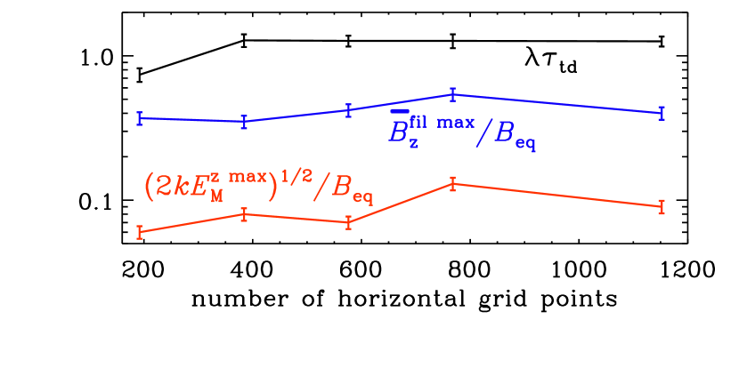
Figure 1: Growth rate $\lambda$ (black line), the peak spectral magnetic field $(2k_{\ast}E_{\rm M}^{z,\max})^{1/2}$ (red), and the maximum of the Fourier-filtered vertical magnetic field $\overline{B}{}_{z}^{\rm fil\,max}$ (blue) for Runs A1-A5 at different resolutions.

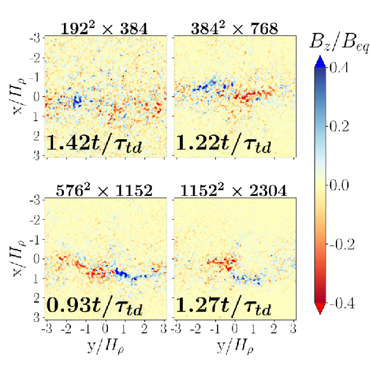
Figure 2: Vertical magnetic field $B_{z}$ at the surface for runs with different resolution (Run A1 to Run A3 and A5) at the time when the structures are strongest.

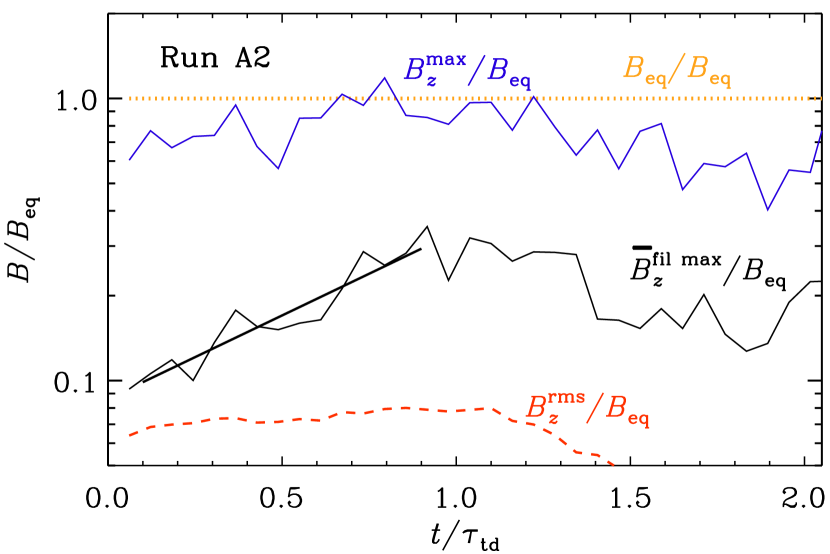
Figure 3: Evolution of $\overline{B}_{z}^{\max}/B_{\rm eq}$ vs. $t/\tau_{\rm td}$ for Run A2 showing exponential growth with growth rate $\lambda=1.3\tau_{\rm td}^{-1}$ (black solid line), compared with that of $B_{z}^{\rm rms}/B_{\rm eq}$ (red dashed line) and $B_{z}^{\max}/B_{\rm eq}$ (blue solid line) at $z=0$. We also show the unity line corresponding to $B_{\rm eq}$ (orange dotted line).

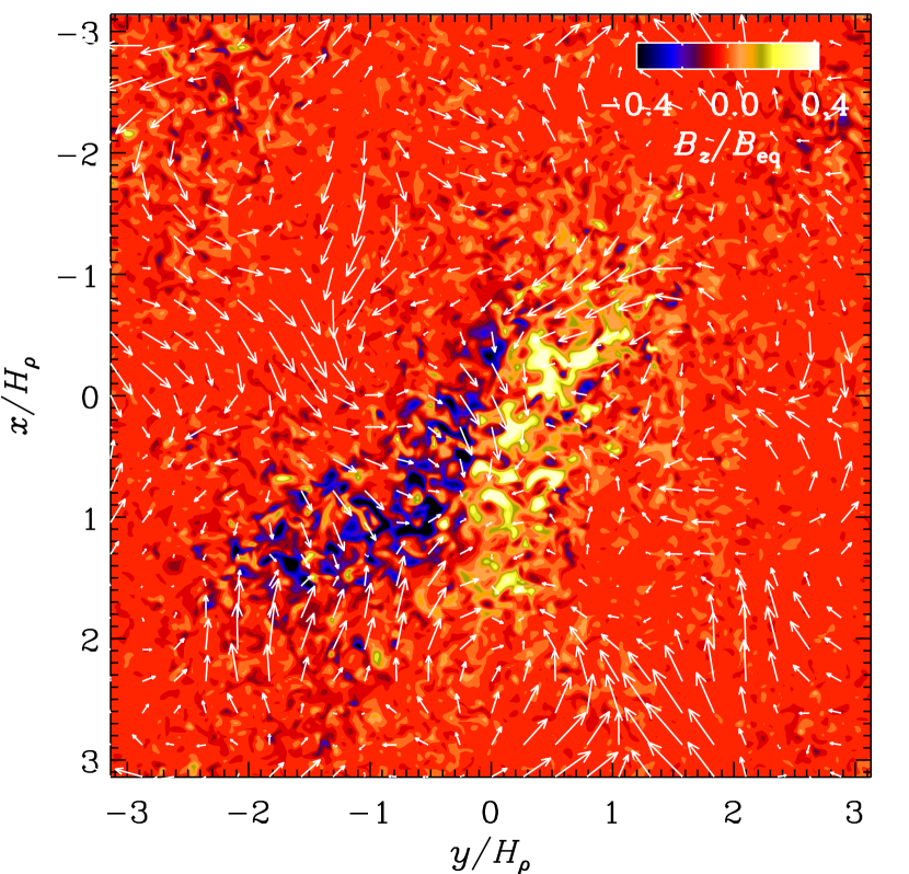
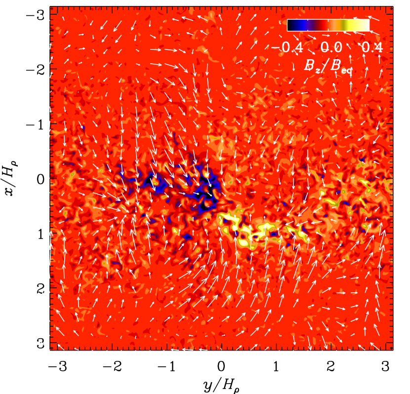
Figure 4: Vectors of the mean (Fourier-filtered) flow superimposed on a color scale representation of $B_{z}$ at the surface at $t/\tau_{\rm td}=0.91$ for Run A4 (upper panel) and $t/\tau_{\rm td}=1.12$ for Run A5 (lower panel). Note that the coordinate system has been rotated by $90\hbox{${}^{\circ}$}$, so $y$ points to the right and $X$ points downward.

We see formation of bipolar regions (denoted by BR in the table) in all the cases, but at the lowest resolution, the growth rate of the magnetic field is significantly smaller than at all higher resolutions. Based on this, we conclude that a resolution of $384^{2}\times 768$ meshpoints results in a good compromise between accuracy and computational cost. Therefore, we use simulations with this resolution for the following parameter study. Because of this reason, Warnecke et al. (2016b) doubled their resolution in their followup work in Warnecke et al. (2013b). Qualitatively, the coherence increases with increasing resolution; see Fig. 2. We see from Table LABEL:runs1 the structures become strongest at a resolution of $768^{2}\times 1536$ meshpoints, where the normalized Fourier-filtered vertical magnetic field at the surface, $\overline{B}{}_{z}^{\rm fil\,max}/B_{\rm eq0}$, reaches a value of 0.54 corresponding to only 0.4 at both lower and higher resolutions.

3.2 Growth of BRs

We now discuss the main properties of BRs. Large-scale BRs form during the first one or two turbulent-diffusive times. They are referred to as large-scale structures, because their size is that of many turbulent eddies (about $2\pi/k_{\rm f}$ in the horizontal plane); see Fig. 4. To average over these turbulent eddies and still resolve the large-scale structure of the BRs, we Fourier-filter the magnetic field at the surface. To investigate the growth of these structures we then plot the maximum of the vertical Fourier-filtered magnetic field $\overline{B}{}^{\rm fil}_{z}$ over time. In Fig. 3, which corresponds to Run A2, we clearly see an exponential growth with growth rate $\lambda\approx 1.3\,\tau_{\rm td}^{-1}$. A similar growth has been seen before in numerical experiments both with a horizontally imposed field (Brandenburg et al. 2011; Kemel et al. 2012a) and a vertical one (Brandenburg et al. 2013). A similar value has also been determined with the same setup, where BRs form (Warnecke et al. 2016b). Such exponential growth is suggestive of NEMPI.

In Fig. 3, we also show for comparison the evolution of the maximum of the surface vertical magnetic field $B^{\rm max}_{z}$, i.e., not the filtered value. Its value is always close to the local equipartition field strength. No exponential growth phase can be seen in the temporal evolution of $B^{\rm max}_{z}$. Likewise, the rms value of surface vertical magnetic field $B_{z}^{\rm rms}=\langle B^{2}_{z}(z=0)\rangle_{xy}^{1/2}$ is about 20 times smaller and shows no exponential growth.

The formation of BRs in our simulations are associated with large-scale flows. As for the magnetic field, we perform Fourier filtering to averaged over the turbulent scales. In Fig. 4 we show these Fourier-filtered large-scale flows that includes only wavenumbers below $k_{\rm f}/6$. The two panels are for Runs A4 and A5 with two different resolutions, but otherwise the same as Run A2, and similar times. In both cases there are BRs, but in one case the two spots are more separated from each other. Nevertheless, in all cases the BRs are surrounded by a large-scale inflow with relative rms value $\overline{U}_{\rm hor}^{\rm rms}/u_{\rm rms}=0.16$–$0.18$, where $\overline{U}_{\rm hor}^{\rm rms}=\langle U_{x}^{2}+U_{y}^{2}\rangle_{xy}^{1/2}$. Its maximum value is around $0.4$. Given that the scale of the turbulent motions is much smaller than the scale of the spots, and that there is otherwise no mechanism producing large-scale flow perturbations, the inflow can only be a consequence of the magnetic field itself, and not the other way around. This is indeed also what one expects for NEMPI.

Another diagnostics for the formation of magnetic structures in our simulations are magnetic power spectra taken at the surface. In Fig. 5 we can see the time evolution of such power spectra. At early times when there are no structures yet, the spectrum peaks at the energy injection wavenumber, $k_{\rm f}=30\,k_{1}$. As time evolves and structures start forming near the surface, magnetic energy is transported toward smaller wavenumbers. When we see the BRs forming at the surface, the magnetic power spectrum peaks at $k=k_{\ast}\approx 2k_{1}$, and the amplitude at this wavenumber decreases until the structures disappear. The strength of the magnetic surface structures at this wavenumber is characterized by the value of $(2kE_{\rm M}^{z,\max})^{1/2}$ at $k=k_{\ast}=2\,k_{1}$; see Sect. 2.1. The resulting values are listed in Tables LABEL:runs1–LABEL:runs3. In addition, we also give the spectral values averaged over the first four wavenumbers from $k/k_{1}=1$ to $4$. The averaging helps reducing the sensitivity to discretization noise that arises from looking at just one wavenumber $k_{\ast}$. In the tables, we also judge BR formation as yes, no, or weak. These attributes are based on the qualitative assessment of images of $B_{z}$.

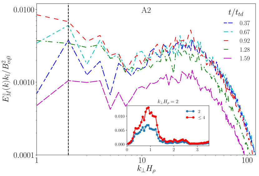
Figure 5: Power spectra of $B_{z}$ at the surface ($z=0$) for Run A2 at several times around the maximum growth for zero rotation. The inset shows the time dependence (time in units of $\tau_{\rm td}$) for $k=k_{\ast}=2\,k_{1}$ and for the values averaged between $k/k_{1}=1$ and $4$.

Table 2: Summary of runs with different Coriolis numbers and colatitudes.

Run Co $\theta$ $\overline{B}{}_{z}^{\rm fil\,max}/B_{\rm eq0}$ $\tau_{\rm td}^{\overline{B}_{z}=\max}$ $\sqrt{2k_{\ast}E_{\rm M}^{z,\max}}/B_{\rm eq0}$ $\tau_{\rm td}^{E_{\rm M}^{z}=\max}$ $\lambda\tau_{\rm td}$ ${\cal P}_{\rm eff}^{\rm min}$ BR A2 0 0 0.35 0.9 0.08 (0.11) 0.92 (0.9) $1.28\pm 0.13$ $-0.029$ yes B1 0.0012 0 0.31 0.8 0.17 (0.22) 0.61 (0.61) $1.32\pm 0.20$ $-0.029$ yes B2 0.0012 30 0.35 0.9 0.13 (0.18) 0.61 (0.73) $1.37\pm 0.11$ yes B3 0.0012 60 0.32 1.7 0.16 (0.20) 0.67 (0.67) $1.46\pm 0.16$ yes B4 0.0012 90 0.42 1.8 0.13 (0.16) 0.73 (0.67) $0.58\pm 0.06$ yes C1 0.0023 0 0.672 1.7 0.30 (0.42) 1.59 (1.59) $1.03\pm 0.07$ $-0.025$ yes C2 0.0023 30 0.303 0.8 0.12 (0.16) 0.61 (0.61) $1.46\pm 0.19$ $-0.021$ yes C3 0.0023 60 0.428 1.7 0.18 (0.26) 1.65 (1.65) $0.66\pm 0.06$ $-0.019$ yes C4 0.0023 70 0.341 2.4 0.12 (0.16) 3.18 (1.96) $0.24\pm 0.05$ yes C5 0.0023 90 0.467 2.0 0.14 (0.20) 1.16 (1.96) $0.64\pm 0.06$ $-0.020$ yes D1 0.0029 0 0.532 1.41 0.26 (0.38) 1.16 (1.28) $1.40\pm 0.17$ $-0.028$ yes D2 0.0029 60 0.406 2.63 0.16 (0.22) 1.16 (1.96) $0.37\pm 0.05$ yes E1 0.0035 0 0.228 0.6 0.11 (0.15) 0.9 (0.9) $0.92\pm 0.3$ $-0.023$ yes E2 0.0035 60 0.241 1.1 0.13 (0.16) 0.5 (0.5) $0.56\pm 0.1$ weak F1 0.0076 0 0.296 1.4 0.11 (0.14) 1.5 (1.5) $0.38\pm 0.09$ $-0.029$ weak F2 0.0076 30 0.269 3.0 0.12 (0.16) 1.8 (1.8) $0.17\pm 0.05$ yes F3 0.0076 60 0.226 0.5 0.11 (0.14) 0.3 (0.3) $0.16\pm 0.13$ no F4 0.0076 90 0.209 0.7 0.11 (0.15) 0.8 (0.8) $0.60\pm 0.15$ weak

Table 3: Summary of runs with different values of imposed field and Coriolis number.

Run $B_{0}/B_{\rm eq0}$ Co $\overline{B}{}_{z}^{\rm fil\,max}/B_{\rm eq0}$ $\tau_{\rm td}^{\overline{B}_{z}=\max}$ $\sqrt{2k_{\ast}E_{\rm M}^{z,\max}}/B_{\rm eq0}$ $\tau_{\rm td}^{E_{\rm M}^{z}=\max}$ $\lambda\tau_{\rm td}$ ${\cal P}_{\rm eff}^{\rm min}$ BR A2 0.026 0 0.35 0.9 0.08 (0.11) 0.92 (0.9) $1.28\pm 0.13$ $-0.029$ yes G1 0.065 0.002 0.38 0.4 0.32 (0.40) 0.49 (0.55) $1.21\pm 0.20$ $-0.046$ yes G2 0.066 0.004 0.54 0.9 0.32 (0.46) 0.73 (0.73) $1.27\pm 0.12$ $-0.041$ yes G3 0.066 0.006 0.52 1.6 0.38 (0.52) 1.59 (1.59) $0.67\pm 0.05$ $-0.039$ yes G4 0.067 0.012 0.50 2.5 0.38 (0.50) 1.34 (1.34) $0.50\pm 0.06$ $-0.048$ yes G5 0.066 0.015 0.46 1.3 0.32 (0.42) 0.98 (1.89) $0.34\pm 0.07$ weak G6 0.068 0.018 0.43 1.4 0.28 (0.34) 0.98 (0.98) $0.33\pm 0.06$ $-0.036$ no H1 0.13 0.002 0.50 0.8 0.28 (0.38) 0.5 (0.3) $0.55\pm 0.09$ $-0.069$ yes H2 0.14 0.006 0.49 0.5 0.32 (0.42) 0.5 (0.5) $0.22\pm 0.13$ $-0.070$ yes H3 0.14 0.012 0.63 2.3 0.44 (0.64) 0.7 (2.1) $0.20\pm 0.03$ $-0.067$ yes H4 0.14 0.018 0.54 3.0 0.32 (0.54) 3.5 (0.9) $0.09\pm 0.04$ $-0.068$ weak I1 0.27 0.002 0.59 0.4 0.24 (0.34) 0.4 (0.4) $0.50\pm 0.52$ $-0.12$ yes I2 0.28 0.006 0.61 0.4 0.44 (0.58) 0.4 (0.4) $0.56\pm 0.29$ $-0.12$ yes I3 0.29 0.013 0.56 1.0 0.42 (0.64) 0.6 (0.5) $0.21\pm 0.08$ $-0.12$ weak I4 0.30 0.019 0.59 1.0 0.42 (0.74) 0.7 (1.0) $0.15\pm 0.07$ $-0.12$ very weak J1 0.77 0.003 0.69 0.05 0.20 (0.28) 0.22 (0.22) $0.10\pm 0.29$ $-0.15$ very weak J2 0.82 0.007 0.64 0.21 0.21 (0.26) 0.32 (0.32) $0.05\pm 0.10$ $-0.16$ very weak J3 0.91 0.014 0.69 0.37 0.23 (0.30) 1.31 (1.31) $0.02\pm 0.12$ $-0.15$ no J4 0.91 0.021 0.73 0.73 0.31 (0.38) 1.36 (1.36) $0.03\pm 0.10$ $-0.16$ no

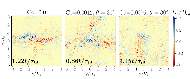
Figure 6: Rotational dependency on the active region formation. We show the vertical magnetic field $B_{z}/B_{\rm eq}$ for Runs A2, B2 and F2 corresponding to $\mbox{\rm Co}=0$, $0.0012$, $0.0076$ at the time of the strongest BR. In the first panel for $\mbox{\rm Co}=0$, the value of $\theta$ is insignificant.

The energy transfer to larger scales is reminiscent of an inverse cascade. Brandenburg et al. (2014) have speculated that such a cascade might be a consequence of the conservation of cross helicity, $\overline{\mbox{\boldmath$u$}{}\cdot\bm{b}}$, where the overbar denotes horizontal averaging, $\bm{b}=\bm{B}-\overline{\mbox{\boldmath$B$}}{}$ are the magnetic fluctuations and $\mbox{\boldmath$u$}{}=\mbox{\boldmath$U$}{}-\overline{\mbox{\boldmath$U$}}{}$ are the velocity fluctuations; see Rüdiger et al. (2011). (For horizontal averages, we usually have $\overline{\mbox{\boldmath$U$}}{}=0$.) They studied the production of $\overline{\mbox{\boldmath$u$}{}\cdot\bm{b}}$ as a result of a mean magnetic field along the direction of gravity, so there exists a pseudoscalar $\mbox{\boldmath$g$}{}\cdot\bm{B}_{0}$ that has the same symmetry properties as $\overline{\mbox{\boldmath$u$}{}\cdot\bm{b}}$ and is also odd in the magnetic field. A similar result was also obtained by Kleeorin et al. (2003); see their Eq. (11) where they considered inhomogeneous turbulence. Furthermore, recent work of Zhang & Brandenburg (2018) has shown that the cross helicity spectrum shows a steep slope at large scales. This was interpreted as a potential signature of NEMPI-like effects.

3.3 Influence of rotation

The structure of the bipolar regions is strongly influenced by rotation; see Fig. 6. Faster rotation causes the magnetic flux concentrations to be weaker. In some cases, for example in Run B3 (middle panel of Fig. 6), the structure of BRs splits into three parts with one negative and two positive polarities. In our most rapidly rotating case (right-most panel of Fig. 6), the structure appears rotated by $90\hbox{${}^{\circ}$}$ with respect to slower rotations.

Table LABEL:runs2 shows that, as the Coriolis number is increased from 0.0012 to 0.0076, BR formation gets almost entirely suppressed (see Runs B1 to F4). At $\theta=0\hbox{${}^{\circ}$}$ (corresponding to the pole), BR formation tends to be slightly easier; but as the Coriolis number is increased, the BRs become clearer at intermediate latitudes.

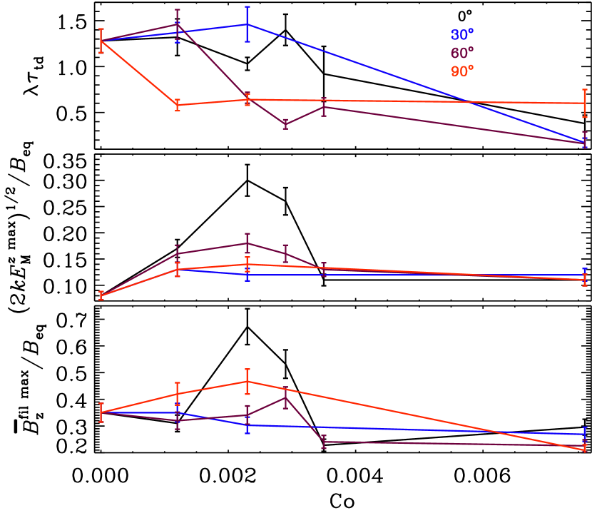
Figure 7: Rotational dependency of the growth rate $\lambda$, the peak spectral magnetic field $(2k_{\ast}E_{\rm M}^{z,\max})^{1/2}$, and the maximum of the Fourier-filtered vertical magnetic field $\overline{B}{}_{z}^{\rm fil\,max}$ for colatitudes $0^{\circ}$ (black line), $30^{\circ}$ (blue line), $60^{\circ}$ (purple line), and $90^{\circ}$ (red line). The error bars are either the errors of the exponential fit ($\lambda$; see Table LABEL:runs2), or estimated as $10\%$ of the actual value.

The rotational dependency of the growth rate $\lambda$ for different colatitudes $\theta$ is shown in Fig. 7. For most of the colatitudes, the growth rate first increases for weak rotation and then gets reduced to around a third of the values for more rapid rotation. Even though we cannot visually detect any clear indication of BRs in the rapidly rotating runs, the growth rate of magnetic field is still positive. The magnetic field strength determined from the spectral energy (see middle panel of Fig. 7) shows actually an enhancement with rotation. Even for the rapidly rotating cases, the magnetic field strength in the flux concentrations is stronger than without any rotation. The strongest values are achieved with $\mbox{\rm Co}=0.002$. For most of the colatitudes, the maxima of the large-scale magnetic field, as shown in the bottom row of Fig. 7, decrease for increasing rotation, similarly as the $\lambda$. However, we see the maximum value for $\mbox{\rm Co}=0.002$ to $0.003$.

The time when the Fourier-filtered magnetic field and the field of spectral energy become maximal depends on rotation, but there is no clear trend visible; see Tables LABEL:runs2 and LABEL:runs3. However there seems to be an indication that the time becomes longer, as expected for a smaller growth rate. As the Coriolis number increases, the structures become weaker and it gets more difficult to discern a clear rotation pattern.

We note here that, unlike in convection, the energy-carrying length scale is not influenced by rotation, because the driving scale is prescribed through the forcing function. Similarly, the kinetic energy is also only weakly influenced by rotation, so $u_{\rm rms}$ decreases only weakly for more rapid rotation.

3.4 Dependence on latitude

As we change the colatitude $\theta$, the growth rates and the strengths of BRs change. This is demonstrated in Fig. 8, where we show $\lambda\tau_{\rm td}$, $(2k_{\ast}E_{\rm M}^{z,\max})^{1/2}/B_{\rm eq0}$ and $\overline{B}{}_{z}^{\rm fil\,max}/B_{\rm eq0}$ for $\mbox{\rm Co}=0.0012$ (corresponding to $2\Omega/\lambda_{\ast 0}\approx 0.15$) and different values of $\theta$. For $\theta=0$, which corresponds to the pole, the saturation magnetic field strength shows a maximum at $t/\tau_{\rm td}\approx 1$. For larger values of $\theta$, i.e., closer to the equator, the maximum is slightly higher (about 0.8) and more long-lived, e.g., for $0.5\leq t/\tau_{\rm td}\leq 2.5$ at $\theta=60\hbox{${}^{\circ}$}$, when $\overline{B}_{z}^{\rm rms}/B_{\rm eq}$ is above 0.6 and sometimes even 0.8.

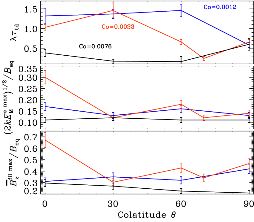
Figure 8: Summary of the results for the different colatitudes showing the normalized growth rate of the Fourier-filtered $z$-component of the magnetic field (top panel) for $B_{0}/B_{\rm eq0}=0.02$, the averaged magnetic spectrum over $k\leq 4$ (middle panel) and the maximum of the Fourier-filtered vertical magnetic field $\overline{B}{}_{z}^{\rm fil\,max}$ (bottom panel) for different values of the Coriolis number and colatitude. As elsewhere, error bars are either the errors of the exponential fit ($\lambda$; see Table LABEL:runs3), or estimated as $10\%$ of the actual value.

Bipolar structures are still fairly pronounced at $\theta=60\hbox{${}^{\circ}$}$, i.e., at $30\hbox{${}^{\circ}$}$ latitude; see Fig. 9. It is remarkable that for all values of $\theta$, the inclination of BRs is approximately the same. The same feature is also seen in the MFS, except that for $\theta=90\hbox{${}^{\circ}$}$ the structures are always aligned in the $y$ direction. This may here be the case, too, but the structures are so weak that this is hard to see. For somewhat faster rotation, when $\mbox{\rm Co}>0.01$, corresponding to $2\Omega/\lambda_{\ast 0}\approx 1$, the structures disappear.

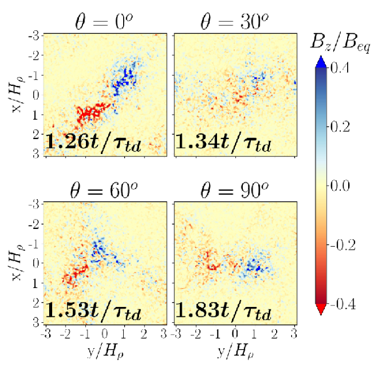
Figure 9: Vertical surface magnetic field $B_{z}/B_{\rm eq}$ for Runs C1–C3 and C5 with $\mbox{\rm Co}=0.0012$.

3.5 Inclination of BRs

A systematic orientation of BRs was already seen in the original papers of Losada et al. (2012, 2013) both for MFS and DNS. For most of the runs, the BRs are either aligned with the imposed magnetic field or they are inclined by $45^{\circ}$. To compare with the Sun, we map our Cartesian coordinate system to spherical ones via $(x,y,z)\to(\theta,\phi,r)$, so the $y$ coordinate points in the toroidal (eastward) direction and $x$ corresponds to colatitude, which points southward. This explains the orientations of our surface visualizations where we plot $-x$ versus $y$; see Fig. 9.

We usually find that rotation leads to a poleward tilt of the BR. We return to the question of the inclination angle in Sect. 4.4 where we study a similar phenomenon in MFS and show that the inclination angle is then not an artifact of the domain size. Note also that the orientation is the same in DNS and MFS. In fact, the orientation agrees with that found by Losada et al. (2012, 2013). It is interesting to note that the sense of inclination is the other way around than what is expected based on the buoyant rise of magnetic flux tubes, which gives rise to Joy’s law (Choudhuri & Gilman 1987).

The “anti-Joy’s” law orientation of NEMPI structures is likely a consequence of the interaction of rotation with the concentration of flux as opposed to the expansion of flux, which is usually expected as a flux tube rises through a stratified layer. A similar phenomenon of a concentration of flux in stratified turbulence (as opposed to an expansion) has been found in turbulence driven by the magneto-rotational instability, where this was argued to be the reason for an unconventional sign of the $\alpha$ effect (Brandenburg et al. 1995); see the more detailed discussion of Brandenburg & Campbell (1997).

3.6 Dependence on the imposed magnetic field strength

Rotation weakens the formation of structures for even smaller Coriolis numbers than those of previous studies (Losada et al. 2012, 2013). We can therefore increase the efficiency of the formation mechanism by increasing the imposed magnetic field, as was suggested by Warnecke et al. (2016b). The increase in the imposed field allows the BRs to be formed for even higher Coriolis numbers, up to the point where the magnetic field becomes so strong that the derivative ${\rm d}{}{\cal P}_{\rm eff}/{\rm d}{}\overline{B}{}^{2}$ becomes positive and NEMPI cannot be excited in the domain; for details, see Brandenburg et al. (2016) and the appendix of Kemel et al. (2013).

Table LABEL:runs3 shows simulations of domains located at the pole ($\theta=0\hbox{${}^{\circ}$}$) and gives their dependence on the magnetic field strength and angular velocity. As $B_{0}/B_{\rm eq0}$ is doubled from 0.07 to 0.14, BR formation becomes slightly easier: compare model G6 with model H4 (both are for $\mbox{\rm Co}=0.018$). Weak BR formation is only possible in model H4. For even stronger fields, however, this trend disappears. In model I4 with $B_{0}/B_{\rm eq0}=0.3$, BR formation is now very weak and for $\mbox{\rm Co}=0.019$, and in model J3 with $B_{0}/B_{\rm eq0}=0.9$, BR formation is impossible—even for $\mbox{\rm Co}=0.014$; see Table LABEL:TCoB0Beq0 for an overview.

Table 4: Comparison of BR formation as a function of rotation in terms of Co and imposed magnetic field $B_{0}/B_{\rm eq0}$.

$B_{0}/B_{\rm eq0}$ Co 0.07 0.14 0.3 0.8 0.0 yes yes no 0.002 yes yes yes very weak 0.006 yes yes yes very weak 0.012 yes yes weak no 0.018 no weak very weak no

The growth rate of the magnetic field shows a strong decrease for higher rotation rates. This can be compensated for to some extent by using a stronger imposed magnetic field; see the top panel of Fig. 10. For $\mbox{\rm Co}\approx 0.006$, the growth rates with imposed magnetic fields of $B_{0}/B_{\rm eq}=0.066$ and $B_{0}/B_{\rm eq}=0.28$ are indeed higher than for $B_{0}/B_{\rm eq}=0.026$. A similar behavior can be found by looking at the magnetic field strength determined from the spectral energy (see middle panel of Fig. 10). For imposed magnetic field strengths between $B_{0}/B_{\rm eq}=0.066$ and $0.85$, the magnetic field is not much influenced by rotation and stays roughly constant above $\mbox{\rm Co}\approx 0.006$ at a level that is even higher than for smaller rotation. The large-scale magnetic field $\overline{B}{}_{z}^{\rm fil\,max}$ for imposed magnetic fields larger than $B_{0}/B_{\rm eq}=0.06$ does not show a strong rotational influence. The large-scale magnetic field is higher for larger imposed magnetic field and keeps this level for a large range of rotation rates. This means that a higher imposed magnetic field can indeed prevent NEMPI from being quenched for larger rotation rates. Even with a large imposed magnetic field, rotational quenching takes place, but at larger rotation rates.

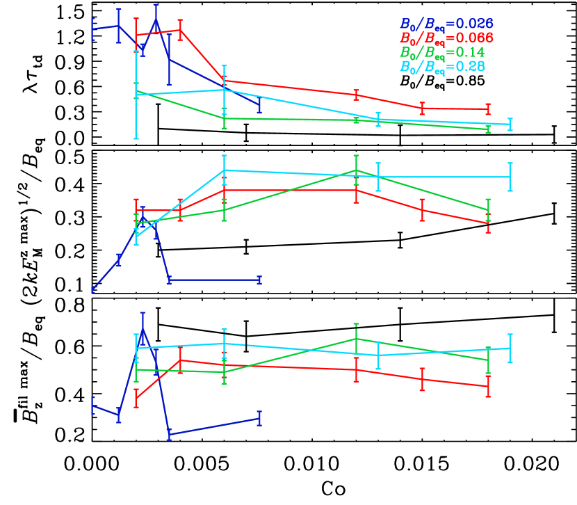
Figure 10: Rotational dependency of the growth rate $\lambda$, the peak spectral magnetic field $(2k_{\ast}E_{\rm M}^{z,\max})^{1/2}$, and the maximum of the Fourier-filtered vertical magnetic field $\overline{B}{}_{z}^{\rm fil\,max}$ for various averaged imposed magnetic field strengths $B_{0}/B_{\rm eq}=0.026$ (blue line), $0.066$ (red), $0.14$ (green), $0.28$ (cyan), and $0.85$ (black). Error bars denote either the errors of the exponential fit ($\lambda$; see Table LABEL:runs2), or are estimated as $10\%$ of the actual value.

3.7 Effective magnetic pressure

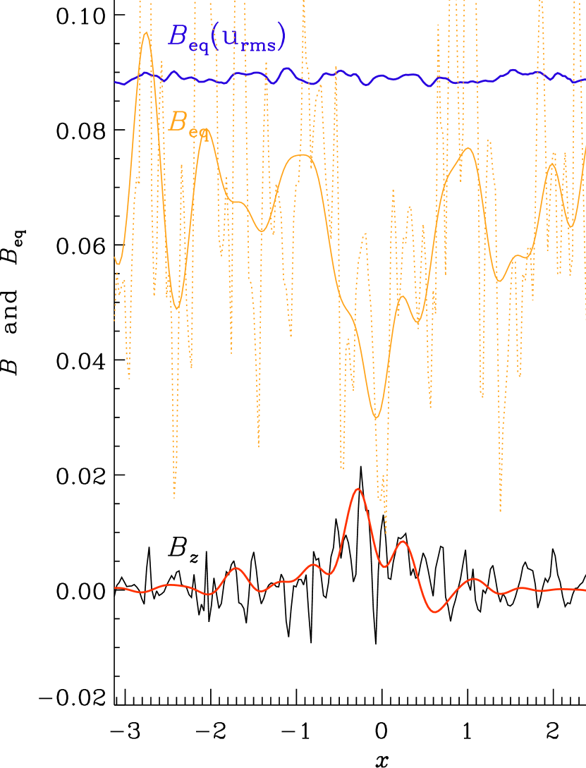
Figure 11: Profiles of $B_{\rm eq}$ and $B_{z}$ at $z=0$ (i.e., the surface of the turbulent region), for Run B1 with $\mbox{\rm Co}=0.0015$, $\theta=0$ at $t/\tau_{\rm td}=1$ and along $y=0$ (black line). The red solid line gives the Fourier-filtered profiles of $B_{z}$. The dotted orange line gives the values of $B_{\rm eq}$ through the magnetic structure and the solid orange lines denotes its Fourier-filtered value. The blue line represents the value of $B_{\rm eq}$ based on the volume-averaged velocity, but the local density. All values have been normalized by the volume-averaged value of $B_{\rm eq}$.

The concentration of magnetic field in a NEMPI scenario is possible due to a turbulence effect on the effective magnetic pressure, which is the sum of non-turbulent and turbulent contributions to the large-scale magnetic pressure. This effect results in a suppression of the total (hydrodynamic plus magnetic) turbulent pressure by the large-scale (mean) magnetic field. This means that an increase of the mean magnetic field due to the instability will be accompanied by a decrease of the turbulent pressure and a reduction of the equipartition field strength, $B_{\rm eq}$. This is because the hydrodynamic part of the total turbulent pressure, $p_{\rm hydro}=\overline{\rho}u_{\rm rms}^{2}/3=B_{\rm eq}^{2}/3$, as well as the turbulent kinetic energy density, decrease due to an increase of the turbulent magnetic energy density as well as the turbulent magnetic pressure through tangling magnetic fluctuations (Kleeorin et al. 1996; Rogachevskii & Kleeorin 2007).

Figure 11 shows the profiles of $B_{\rm eq}$ and $B_{z}$ at the surface along $y=0$ at $t/\tau_{\rm td}=1$. This figure clearly shows that at the location of the maximum of the vertical magnetic field, the equipartition field $B_{\rm eq}$ is decreased. Most of this suppression comes from a local decrease in the turbulent velocity, while the local density through the structure varies only little; see the blue line of Fig. 11. We attribute this behavior to the operation of NEMPI in the simulation.

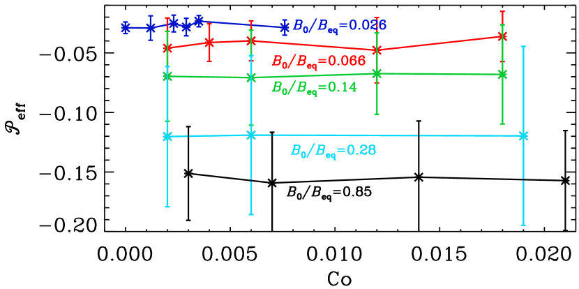
Figure 12: Dependence of the minimum value of the normalized effective magnetic pressure, ${\cal P}_{\rm eff}$, on the Coriolis number for different values of the imposed field strength, $B_{0}/B_{\rm eq0}$ (the curves have been labeled by an average value), for the runs listed in Tables LABEL:runs2 and LABEL:runs3. Again, error bars are estimated using the maximum difference of the total mean with the means of each third of the time series.

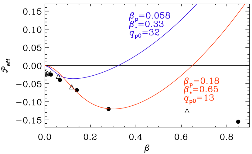
Figure 13: Dependence of ${\cal P}_{\rm eff}(\beta)$ obtained from Fig. 12 by taking an average for different values of Co (filled circles). The blue line is our standard representation for $q_{\rm p0}=32$ and $\beta_{\rm p}=0.058$, which corresponds to $\beta_{\ast}=0.33$, while the red line is a better fit to the present data giving $q_{\rm p0}=13$ and $\beta_{\rm p}=0.18$, which corresponds to $\beta_{\ast}=0.65$. Note that the data point at $\beta=0.85$ and ${\cal P}_{\rm eff}=-0.16$ is well outside any ${\cal P}_{\rm eff}(\beta)$ curve that could fit all the data and has therefore been discarded as an “outlier”. As a comparison, we plot the values of Warnecke et al. (2016b) as triangles.

Next, we determine the normalized effective magnetic pressure, ${\cal P}_{\rm eff}$, as

$${\cal P}_{\rm eff}=(1-q_{\rm p})\,\beta^{2}/2,$$ (18)

where $q_{\rm p}$ is obtained from (Kemel et al. 2013)

$$q_{\rm p}=-{1\over\overline{\bm{B}}^{2}}\,\left(\Delta\overline{\Pi}_{xx}+\Delta\overline{\Pi}_{yy}-\left(\Delta\overline{\Pi}_{xx}-\Delta\overline{\Pi}_{yy}\right)\,{\overline{B}_{x}^{2}+\overline{B}_{y}^{2}\over\overline{B}_{x}^{2}-\overline{B}_{y}^{2}}\right).$$ (19)

Overbars denote here $xy$ averaging and the diagonal components of the total (Reynolds and Maxwell) stress tensor, $\Delta\overline{\Pi}_{ii}$, have been obtained from the DNS as

$$\Delta\overline{\Pi}_{ii}=\overline{\rho}\,(\overline{u_{i}^{2}}-\overline{u_{0i}^{2}})+{\textstyle{1\over 2}}(\overline{\bm{b}^{2}}-\overline{\bm{b}_{0}^{2}})-(\overline{b_{i}^{2}}-\overline{b_{0i}^{2}}),$$ (20)

where the subscript $0$ refers to values for $B_{0}=0$ and lower case letters denote fluctuations, i.e., $\mbox{\boldmath$u$}{}=\mbox{\boldmath$U$}{}-\overline{\mbox{\boldmath$U$}}{}$ and $\bm{b}=\bm{B}-\overline{\mbox{\boldmath$B$}}{}$. No summation over the index $i$ is assumed. In Fig. 12 we show the dependence of the minimum value of ${\cal P}_{\rm eff}$ on the Coriolis number (see Table LABEL:runs2) and for different values of the imposed field (see Table LABEL:runs3). It turns out to be relatively insensitive to the value of Co, but it drops dramatically with increasing strength of the imposed field.

Given that the values of ${\cal P}_{\rm eff}$ shown in Fig. 12 for different values of Co are almost the same, we conclude that those coefficients do not depend on $\Omega$. We can therefore obtain a new set of parameters that is representative of our model with coronal layer and for all values of $\Omega$, which is different from our standard representation without a coronal envelope. This is shown in Fig. 13. The values of the parameters $q_{\rm p0}$ and $\beta_{\rm p}$ fit very well with the data of Warnecke et al. (2016b), shown as triangles.

The new data can be fitted to Eq. (15) by determining the position and value of the minimum, $\beta_{\min}$ and ${\cal P}_{\rm eff}^{\rm min}$, respectively. Looking at Fig. 13, we find $\beta_{\min}\approx 0.3$ and ${\cal P}_{\rm eff}^{\rm min}\approx-0.12$. We then obtain the fit parameters as (Kemel et al. 2012b)

$$\beta_{\rm p}=\beta_{\min}^{2}\left/\sqrt{-2{\cal P}_{\rm eff}^{\rm min}},\right.\;\;\beta_{\star}=\beta_{\rm p}+\sqrt{-2{\cal P}_{\rm eff}^{\rm min}}.$$ (21)

This results in the following new set of parameters: $q_{\rm p0}=13$ and $\beta_{\rm p}=0.18$, which corresponds to $\beta_{\ast}=0.65$. We therefore also present in the next section MFS results based on our model with this parameter combination.

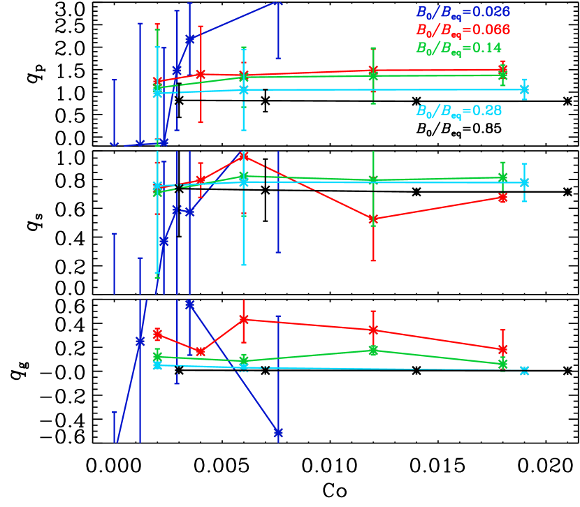
Figure 14: Dependence $q_{\rm p}$, $q_{\rm s}$, and $q_{\rm g}$ on the Coriolis number for different values of the imposed field strength, $\beta_{0}=B_{0}/B_{\rm eq0}$ (the curves have been labeled by an average value), for the runs listed in Tables LABEL:runs2 and LABEL:runs3. Error bars are estimated using the maximum difference of the total mean with the means of each third of the time series.

Along with $q_{\rm p}$ and ${\cal P}_{\rm eff}$, we also determine $q_{\rm s}$ and $q_{\rm g}$ in

$$\Delta\overline{\Pi}_{ij}=-q_{\rm p}\delta_{ij}{\overline{\bm{B}}^{2}\over 2}+q_{\rm s}\overline{B}_{i}\overline{B}_{j}-q_{\rm g}{g_{i}g_{j}\over g^{2}}\overline{\bm{B}}^{2},$$ (22)

resulting in

$$q_{\rm s}={\Delta\Pi_{xx}-\Delta\Pi_{yy}\over\overline{B}_{x}^{2}-\overline{B}_{y}^{2}},$$ (23)

$$q_{\rm g}={1\over\overline{\bm{B}}^{2}}\,\left(-\Delta\Pi_{zz}-q_{\rm p}{\overline{\bm{B}}^{2}\over 2}+q_{\rm s}\overline{B}_{z}^{2}\right),$$ (24)

where ${g_{i}}$ are components of $g$ which, in our setup, has only a component in the negative $z$ direction. In Fig. 14 we plot the dependencies of $q_{\rm p}$, $q_{\rm s}$, and $q_{\rm g}$ on angular velocity and imposed magnetic field strength. The values for no and weak rotation are consistent with those obtained by Warnecke et al. (2016b) for a non-roting setup and the same magnetic field strengths. Because of the large errors resulting from the strong variation in space and time, we cannot determine whether the sign is negative or positive. For larger imposed magnetic field strengths, the situation becomes more clear. There, the errors are significantly larger and $q_{\rm p}$, $q_{\rm s}$, and $q_{\rm g}$ do not strongly depend on rotation. However, we see a dependence on the imposed magnetic field strength. In particular, $q_{\rm p}$ is positive for $B_{0}/B_{\rm eq0}\geq 0.066$ and decreases from around $1.5$ to $1.0$ for increasing imposed magnetic field strength. Next, $q_{\rm s}$ is also positive for imposed magnetic fields $B_{0}/B_{\rm eq0}\geq 0.066$, but has an inconclusive dependence on the imposed magnetic field. Finally, $q_{\rm g}$ is also positive for $B_{0}/B_{\rm eq0}\geq 0.066$, it decreases with increasing imposed field until it is nearly zero for $B_{0}/B_{\rm eq0}=0.85$. For $B_{0}/B_{\rm eq0}=0.066$, $q_{\rm g}$ tends to decrease with increasing angular velocity, but not for the other magnetic field strengths. We should keep in mind that the $q_{\rm p}$ and $q_{\rm g}$ in Eq. (12) are multiplied by the horizontal averaged magnetic field, which will be larger for larger imposed magnetic fields. We also look at the latitudinal dependencies of $q_{\rm p}$, $q_{\rm s}$, and $q_{\rm g}$; see Fig. 15. We do not find any latitudinal dependence of these coefficients, mostly because the errors are so large. In conclusion, we cannot explain the rotational dependence found in the DNS with just the rotational dependence of $q_{\rm p}$, $q_{\rm s}$, and $q_{\rm g}$.

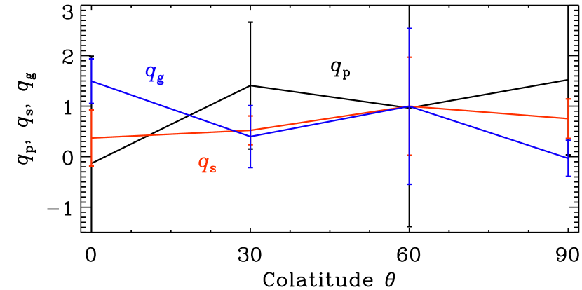
Figure 15: Dependence $q_{\rm p}$, $q_{\rm s}$ and $q_{\rm g}$ on the colatitude $\theta$ for Runs C1–C3 and C5 with Co=0.0023 and $B_{0}/B_{\rm eq0}=0.026$. Error bars are estimated using the maximum difference of the total mean with the means of each third of the time series.

4 MFS results

4.1 General aspects

We now present mean-field calculations with a coronal envelope. In all cases, we use $\nu_{\rm T}=\eta_{\rm T}=10^{-3}c_{\rm s}H_{\rho}$ and $u_{\rm rms}=0.1c_{\rm s}$, corresponding to $k_{\rm f}H_{\rho}=33$, which is similar to the value of $30$ used in the DNS. We first consider the same domain size as in the DNS, i.e., $(2\pi)^{2}\times 3\pi$. To alleviate finite domain size effects, we also consider a wider and deeper domain, but with a smaller coronal part that is reduced by half. We thus also consider $L_{x}=L_{y}=6\pi$, $L_{z}=4\pi$, and $z_{\rm top}=\pi$.

The MFS lack small-scale turbulent motions, so fewer mesh points can be used. However, to resolve the vertical density contrast of around 12,000, we used 288 mesh points in the $z$ direction. For our domains, are used $192^{2}\times 288$ meshpoints, but we found no differences in the results when using $96^{2}\times 288$ meshpoints. For the larger domains, we used $384^{3}$ meshpoints, but again, with fewer meshpoints the results would have been sufficiently accurate. In all cases, we use $B_{0}/B_{\rm eq0}=0.1$, because the DNS discussed in Sect. 3.6 showed that for approximately this value, the range in rotation rates over which NEMPI is still excited would be maximized.

Although we have found that the parameters $q_{\rm p0}\approx 13$ and $\beta_{\rm p}\approx 0.65$ describe the DNS best, there are reasons to consider also other choices. First, there is no good reason why the parameters $q_{\rm p0}$ and $\beta_{\rm p}$ are so different in different circumstances. One would have expected them to reflect properties of the turbulence which is similar in all the different cases. Second, the response for vertical and horizontal magnetic fields turns out to be different; see Fig. 7 of Losada et al. (2014). There are also other differences between MFS and DNS that we address below. Thus, we cannot expect the two approaches to agree. One objective is therefore to find out just how well the MFS perform relative to the DNS.

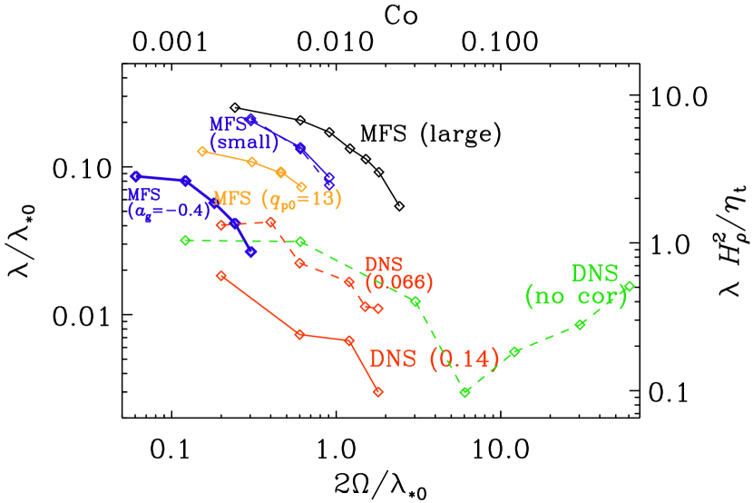
Figure 16: Dependence of $\lambda/\lambda_{\ast 0}$ on $2\Omega/\lambda_{\ast 0}$ for $B_{0}/B_{\rm eq0}=0.1$ and $\theta=0$ for the MFS using the large (black line) and small domains (blue solid line), as well as the DNS for neighboring magnetic field strength of $B_{0}/B_{\rm eq0}=0.066$ and 0.14 (dashed and solid red lines, respectively). The fat blue line denotes the case of a small domain using $a_{\rm g}=-0.4$ instead of $0$. The green dashed line denotes the DNS of Losada et al. (2013) without coronal layer and $B_{0}/B_{\rm eq0}=0.05$. The orange line refers to MFS in a small domain with $q_{\rm p0}=13$ and $\beta_{\rm p}=0.18$, so $\beta_{\ast}=0.65$. The blue dashed line adjacent to the blue solid line denotes the results obtained when neglecting the derivative term of the profile function $\Theta_{w}(z)$.

4.2 Growth rates

In the DNS, the value of $\lambda/\lambda_{\ast 0}$ is found to drop by about a factor of five as $2\Omega/\lambda_{\ast 0}$ increases from 0.2 to 3; see Fig. 16. We compare the MFS for $B_{0}/B_{\rm eq0}=0.1$ with the DNS at $B_{0}/B_{\rm eq0}=0.066$ and $0.14$; see Table LABEL:runs2. We also compare with the DNS of Losada et al. (2013) without coronal envelope using $\beta_{\ast}=0.33$ and, as in Losada et al. (2013), the value $\beta_{\ast}=0.75$, which was suitable for one of their sets of MFS. This now explains the 2.3 times larger ratio of $\lambda/\lambda_{\ast 0}$ compared to their Fig. 2. In addition, however, the growth rates of their DNS were incorrectly scaled by a factor $(u_{\rm rms}/c_{\rm s})(k_{\rm f}/k_{1})\approx 0.1\times 30=3$, which is now corrected; see the green line of Fig. 16. Thus, even in the absence of a corona, the growth rates were by a factor of about seven larger in the MFS than in the DNS; see Appendix A with a corrected version of Fig. 2 of Losada et al. (2013).

Again, the growth rates of the large-scale instability in the MFS are significantly larger than those in the DNS. We speculate that this could be caused by a partial cancelation (i.e., a decrease of the effective magnetic pressure gradient) from the $q_{\rm g}$ term in Eq. (12). To illustrate this possibility, we have overplotted in Fig. 16 a case with $a_{\rm g}=-0.4$; see Eq. (13). Given that in Eq. (12), only the $q_{\rm p}$ term comes with a 1/2 factor, the effective magnetic pressure gradient in the $z$ direction is reduced. Thus, $q_{\rm p}/2$ is replaced by $q_{\rm p}/2+q_{\rm g}=(1/2+a_{\rm g})\,q_{\rm p}$, so $q_{\rm p}$ is scaled by a factor $1+2a_{\rm g}=0.2$ with respect to the $z$ direction. We see that the growth rate is now suppressed, but also the maximum rotation rate for which NEMPI can operate is reduced. Obviously, a more accurate modeling requires a more detailed knowledge of the actual form of $q_{\rm g}$, which is likely to be different from that of $q_{\rm p}$. We should also point out that, when calculating $\partial_{z}q_{\rm g}(\beta)$ in Eq. (12), one of the resulting terms involves the gradient of $\Theta_{w}(z)$ in Eq. (14). We have verified that neglecting this term causes only a very minor change in the resulting growth rates; cf. the solid and dashed blue lines in Fig. 16.

Let us discuss the non-monotonic behavior of the growth rate of the magnetic field as a function of the Coriolis number; see Fig. 16. In corresponding DNS without coronal layer (Jabbari et al. 2014), the increase in the growth rate at faster rotation rates ($\mbox{\rm Co}>0.1$ or $2\Omega/\lambda_{\ast 0}>10$) has been explained as a result of large-scale dynamo action; see Fig. 8 of Jabbari et al. (2014). In particular, at larger rotation rates, kinetic helicity is produced by a combined effect of uniform rotation and density stratified turbulence. It results in the excitation of an $\alpha\Omega$ or $\alpha^{2}\Omega$ dynamo instabilities and the generation of a large-scale magnetic field. This causes an increase of the growth rate at larger Coriolis numbers, which is also observed in the DNS of Losada et al. (2013) and Jabbari et al. (2014). This implies that two different instabilities are excited in the system, i.e., NEMPI at low Coriolis numbers and the mean-field dynamo instability at larger values of the Coriolis numbers. This causes a non-monotonic behavior of the growth rate of magnetic field as the function of the Coriolis number, observed in Fig. 16.

A non-trivial evolution of the magnetic field in rotating turbulence with a coronal envelope is caused for the following reasons. In an earlier study by Losada et al. (2012) with rotation, no coronal envelope, and an imposed horizontal magnetic field, an analytical expression for the growth rate of NEMPI has been derived in the framework of a mean-field approach. During the magnetic field evolution in the presence of a coronal envelope, as in the simulation of Warnecke et al. (2013b, 2016b) and the present ones, there is a change in the direction of the large-scale magnetic field from horizontal at $t=0$ to nearly vertical after about one turbulent diffusive time. Therefore, in turbulence with a coronal envelope one can expect to find a mixture of effects caused by the horizontal and vertical magnetic fields.

The growth rates and saturation mechanisms of NEMPI for horizontal and vertical fields are very different (see review by Brandenburg et al. 2016). For horizontal fields, NEMPI saturates rapidly in the nonlinear stage of the magnetic field evolution due to the “potato-sack” effect. This means that a local increase of the magnetic field causes a decrease of the negative effective magnetic pressure, which is compensated for by enhanced gas pressure. This leads to an enhanced gas density, so the gas is heavier than its surroundings and sinks. This effect removes horizontal magnetic flux structures from regions in which NEMPI is excited. For a vertical magnetic field, the heavier fluid moves downward along the field without affecting the flux tube, so that NEMPI is not stabilized by the potato sack effect. In this case the operation of NEMPI results in the formation of strong concentrations (see Brandenburg et al. 2013, 2016).

In the non-rotating cases, the growth rates of the large-scale magnetic field measured in DNS with coronal envelope and horizontal initial field (Warnecke et al. 2016b), and with vertical magnetic field but without corona (Brandenburg et al. 2013), are the same. This is an indication that the growth rates of the large-scale magnetic field in the simulations with coronal envelope are determined by the evolution of the vertical field. On the other hand, the fact that the BRs dissolve after a few turbulent diffusion times is more similar to the behavior of NEMPI with a horizontal imposed magnetic field. Therefore, the evolution of the magnetic structures in the system with coronal envelope is non-trivial and cannot easily be described with our current mean-field models. Therefore, also explaining the rotational dependency of growth rates in this setup suffers from the mixture of effects.

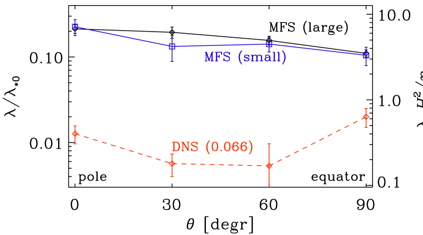
Figure 17: Dependence of $\lambda/\lambda_{\ast 0}$ on $\theta$ for $B_{0}/B_{\rm eq0}=0.1$ and $\mbox{\rm Co}=0.006$.

4.3 Latitudinal dependence

At slower rotation, a decrease in $\lambda/\lambda_{\ast 0}$ can be seen as $\theta$ increases from $\theta=0$ at the poles to $\theta=90\hbox{${}^{\circ}$}$ at the equator; see Fig. 17. In both plots we also show the growth rates for the larger domain, which are found to be enhanced by a factor of two when $2\Omega/\lambda_{\ast 0}\approx 1$. These values are about an order of magnitude larger than those for the DNS, but have otherwise a similar functional dependence on $\Omega$ and $\theta$. The reason for the difference between DNS and MFS is not entirely clear. It is possible that the mean-field parameter $\beta_{\ast}$ is smaller than what was previously found for simulations with coronal envelope. There is also the possibility that $\beta_{\ast}$ decreases with increasing angular velocity, which is what Rüdiger (private communication) found, although our present simulations presented in Fig. 12 and earlier ones of Losada et al. (2013) did not give such indications.

4.4 Inclined surface structures

Next, we show slices of $\overline{B}_{z}(x,y,0,t_{\ast})$ along the surface $z=0$ at a chosen time $t_{\ast}$ during the linear growth phase of NEMPI for three values of Co using domain sizes of $(2\pi)^{2}\times 3\pi$ (Fig. 18) and $(6\pi)^{2}\times 4\pi$ (Fig. 19). In the linear phase, when the magnetic field fluctuations are still growing exponentially in time, only relative values are of physical interest. We therefore present in the following images where the magnetic field is normalized by the maximum value. As in the DNS, the imposed magnetic field points in the $y$ direction. It turns out that rotation not only tends to make the structures inclined relative to the direction of the imposed magnetic field, but it also leads to higher wavenumbers of the structures. Figure 19 shows that the number of nodes in the $x$ direction, which is perpendicular to the magnetic field, remains about constant ($k_{x}L_{x}/2\pi=4$), while that in the $y$ direction along the magnetic field increases from $k_{y}L_{y}/2\pi=1$ (for $\mbox{\rm Co}=0$) to 2 (for $\mbox{\rm Co}=0.006$) and 4 (for $\mbox{\rm Co}=0.018$).

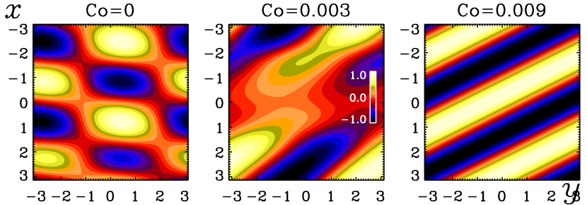
Figure 18: Slices of $\overline{B}_{z}(x,y,0,t_{\ast})$ through the surface $z=0$ at times $t_{\ast}$ during the linear growth phase of NEMPI for $B_{0}/B_{\rm eq0}=0.1$ and three values of Co using the smaller domain size of $(2\pi)^{2}\times 3\pi$. In each panel, the magnetic field is scaled to the maximum value.

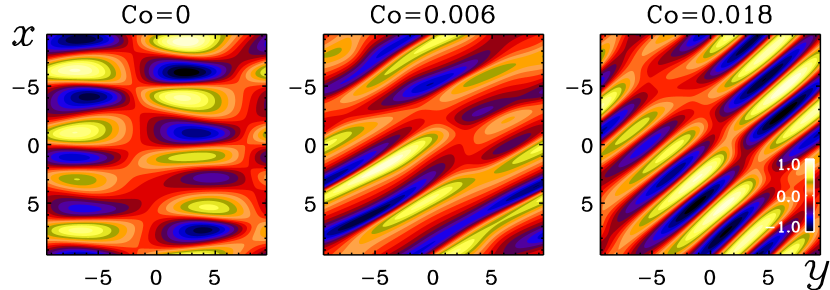
Figure 19: Similar to Fig. 18, but for the large domain, $(6\pi)^{2}\times 4\pi$.

In both the DNS and the MFS, the orientation of the inclination is the same and it is opposite to what is seen in Joy’s law. The runs presented here apply of course only to the poles, but even at lower latitudes (e.g., at $30\hbox{${}^{\circ}$}$ latitude, corresponding to $\theta=60\hbox{${}^{\circ}$}$) do we find the same anti-Joy’s law orientation of the tilt. This is shown in Fig. 20, where we compare two runs with $\theta=80\hbox{${}^{\circ}$}$ (close to the equator) for a section of the large domain and the full section of the smaller domain, as well as a run with $\theta=90\hbox{${}^{\circ}$}$ (at the equator). At the equator, the inclination angle with respect to the toroidal direction is $90\hbox{${}^{\circ}$}$, which agrees with what was found in Losada et al. (2012). However, slightly away from the equator, at $\theta=80\hbox{${}^{\circ}$}$, the inclination angle is already $45\hbox{${}^{\circ}$}$. This is not an artifact of having chosen a small domain, because even for a three times larger domain, the same inclination angle is found. We thus remain puzzled about this finding and hope to be able to return to it as further numerical and analytic results can be obtained and assessed.

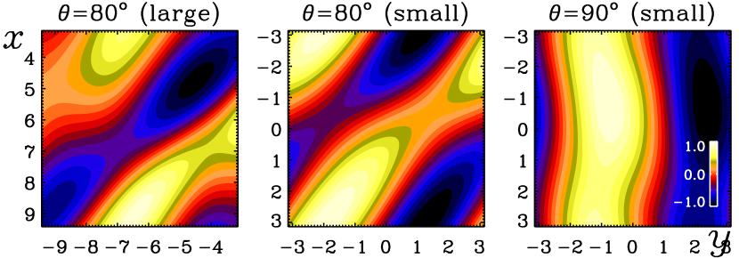
Figure 20: Similar to Fig. 18, but for two runs with $\theta=80\hbox{${}^{\circ}$}$ for a 1/3 section of the large domain and the full section of the smaller domain, as well as a run with $\theta=90\hbox{${}^{\circ}$}$.

One might speculate that the reason for the difference to Joy’s law has to do with the expansion of rising structures whereas NEMPI structures are caused by contraction, which leads to the opposite tilt. Thinking again of possible applications to the Sun, one may therefore wonder whether the effect of flux concentrations in NEMPI, which must also be responsible for causing the tilt, operate on relatively small scales and might be responsible for causing sunspot rotation (Evershed 1909; Kempf 1910; Pevtsov 2012; Sturrock et al. 2015), for example. In a distributed solar dynamo scenario, the tilt of active regions is primarily caused either by differential rotation (Brandenburg 2005) or simply by the sign of the mean latitudinal field $\overline{B}_{\theta}$ relative to that of the azimuthal field $\overline{B}_{\phi}$ (Jabbari et al. 2015).

4.5 Emergence of solitary structures

The magnetic field patterns in Figs. 18–20 are more or less regular. This is basically because those pictures were taken from the linear phase of the run. In Fig. 21 we show a visualization of $\overline{B}_{z}$ along with horizontal flow vectors $(\overline{U}_{x},\overline{U}_{y})$ through the surface for an arbitrarily chosen time $t_{\ast}/\tau_{\rm td}=40$ during the saturated state for the large domain using $\mbox{\rm Co}=0.006$. We can now clearly see solitary structures in the form of isolated spots. However, with a few exceptions, most of these structures lack the distinct bipolarity seen in the DNS. Note also that the mean flow is mostly circular around each spot rather than a convergent inflow, as seen in the DNS.

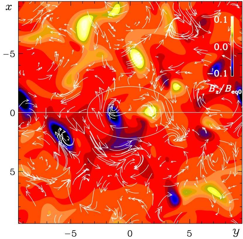
Figure 21: A slice of $\overline{B}_{z}(x,y,z_{\ast},t)$ (color coded) together with velocity field vectors (white streak lines) through $z_{\ast}=0$ at $t_{\ast}/\tau_{\rm td}=40$ during the saturated state for the large domain using $\mbox{\rm Co}=0.006$. The white horizontal line through $x=0$ marks the position of a BR near $y=0$, which is discussed separately. The ellipse marks the position of the BR discussed in the text.

In Fig. 21 we mark with a white horizontal line in the toroidal direction through $x=0$ the position of a BR near $y=0$. Unlike the DNS, the separation of the two polarities is rather large (about $3\,H_{\rho}$) and there are other spots in almost the same distance. Thus, it is not clear that these two polarities are connected to each other. There is also no clear indication of BRs. To examine this further, we present in the next section a side view of this BR.

4.6 Side view of BRs

In Fig. 22 we show a longitudinal cross-section of the magnetic field through $x_{\ast}=0$ at the same time as Fig. 21 during the saturated state. Magnetic flux concentrations are seen to occur at a depth of $z/H_{\rho}\approx-6$, which is well below the surface. Near the surface, on the other hand, there is only a relatively small number of vertical magnetic flux structures that seem to close upon themselves over relatively large horizontal distances. We recognize the positive and negative polarities at $y/H_{\rho}\approx\pm 1.5$ and the negative one at $y/H_{\rho}\approx-8$ in both Figs. 21 and 22. Conversely, over short distances, bipolar magnetic flux structures separate above the surface, which is consistent with them being the result of a localized subduction of a horizontal flux structure.

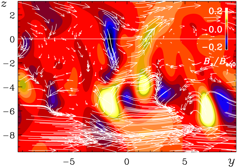
Figure 22: A slice of $\overline{B}_{z}(x_{\ast},y,z,t)$ (color coded) together with magnetic field vectors (white streak lines) through $x_{\ast}=0$ at an arbitrarily chosen time during the saturated state for the large domain. The surface at $z=0$ is shown as a white horizontal line.

To compare with DNS results, we show in Fig. 23 a similar plot of $B_{z}$ together with Fourier-filtered magnetic field vectors in the same plane. A major difference to Fig. 22 is the absence of significant horizontal field in the deeper parts. However, since this horizontal field in the MFS is so deep down ($z/H_{\rho}\mathrel{\mathchoice{\vbox{\offinterlineskip\halign{\hfil$\displaystyle#$\hfil\cr<\cr\sim\cr}}}{\vbox{\offinterlineskip\halign{\hfil$\textstyle#$\hfil\cr<\cr\sim\cr}}}{\vbox{\offinterlineskip\halign{\hfil$\scriptstyle#$\hfil\cr<\cr\sim\cr}}}{\vbox{\offinterlineskip\halign{\hfil$\scriptscriptstyle#$\hfil\cr<\cr\sim\cr}}}}-8$), it is unclear whether it plays any role in explaining the difference in, for example, the growth rates between DNS and MFS seen in Fig. 16. On the other hand, in the deeper parts of the MFS, there are magnetic structures of significant strength, which are not so prominent in the DNS. This is an important difference that would affect global comparisons of, for example, the growth rates of structures shown in Fig. 16.

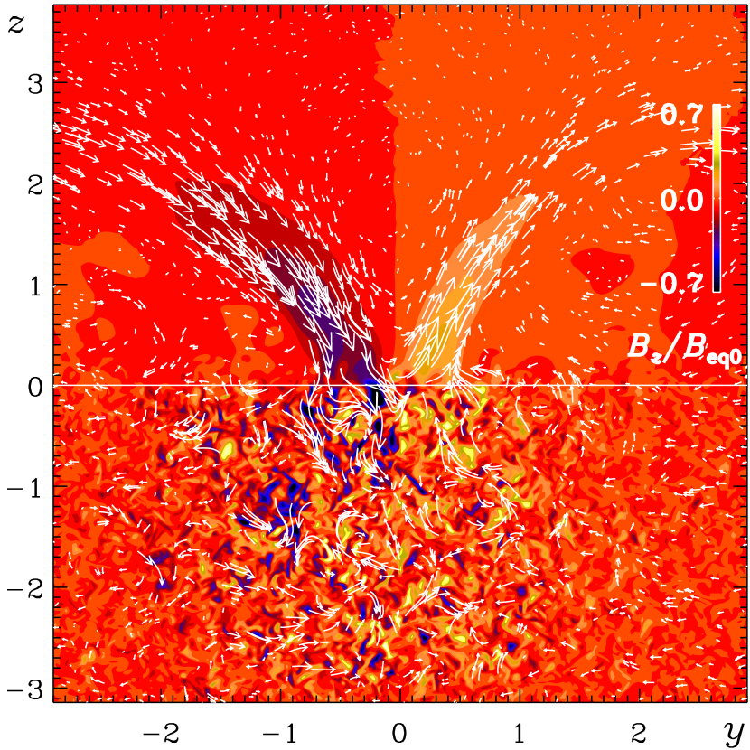
Figure 23: Comparison with DNS showing $B_{z}(x_{\ast},y,z,t)$ (color coded) together with vectors of Fourier-filtered magnetic field vectors ($k<k_{\rm f}/2$) superimposed for Run A4 at the time $t/\tau_{\rm td}=0.91$ through $x_{\ast}=0.5$.

5 Discussion

Our calculations have been performed using idealizing circumstances such as forced turbulence and an isothermal equation of state. This is in many ways different from turbulence in the Sun, which is driven by convection. Nevertheless, some tentative conclusions can be drawn regarding possible applications to sunspot formation. In the surface layers of the Sun, the turnover time $\tau_{\rm to}=H_{p}/u_{\rm rms}$ based on the pressure scale height $H_{p}$ is around $5\min$. Assuming $k_{1}H_{p}=1$, the turbulent diffusive time scale is related to this via

$$\tau_{\rm td}=H_{p}^{2}/\eta_{\rm t0}=3k_{\rm f}H_{p}^{2}/u_{\rm rms}=3k_{\rm f}H_{p}\tau_{\rm to}.$$ (25)

In the simulations, we have $k_{\rm f}H_{p}\approx k_{\rm f}/k_{1}=30$, so $\tau_{\rm td}$ would be about 90 times longer than $\tau_{\rm to}$, i.e., about 8 hours. This would appear suitable in view of applications to the Sun as well, where the formation time of sunspots is of a similar order.

Although the presence of our simplified corona has the effect of allowing BRs to form that reach a significant fraction of the equipartition value with respect to the turbulence, these structures can no longer form when the Coriolis number exceeds a critical value of about 0.02. This value is rather small. However, given that the growth rate of NEMPI does not scale with the inverse turnover time $\tau_{\rm to}^{-1}$, but with the turbulent-diffusive time $\tau_{\rm td}^{-1}$, a meaningful measure of the rotation rate in this context could also be the square root of the turbulent Taylor number, $\mbox{\rm Ta}_{\rm t}^{1/2}=2\Omega/\nu_{\rm t}k_{1}^{2}=3\,(k_{\rm f}/k_{1})^{2}\mbox{\rm Co}$, where we took into account that the turbulent viscosity $\nu_{\rm t}$ is equal to the turbulent magnetic diffusivity $\eta_{\rm t}$ (Yousef et al. 2003; Kleeorin & Rogachevskii 1994) and given by $\eta_{\rm t}\approx u_{\rm rms}/3k_{\rm f}$ (Sur et al. 2008). The values of $\mbox{\rm Ta}^{1/2}$ are typically of the order of 10 when NEMPI begins to be suppressed. Using our estimate of $\tau_{\rm td}=8\,{\rm hours}$ for the solar surface, we find $\mbox{\rm Ta}^{1/2}=0.2$, which is well below our critical value of 10.

In the standard mixing length theory of convection, the value of $k_{\rm f}H_{p}$ is estimated to be around 6–7 (Kemel et al. 2013), but it is about $30$ in the present simulations. Earlier work showed that NEMPI would not work for $k_{\rm f}H_{p}$ much below 15 (Brandenburg et al. 2012). On the other hand, the actual value in the Sun is unclear given that the findings of Hanasoge et al. (2012) did not confirm turbulent velocities in the Sun at the expected levels. A possible resolution to this problem might be the idea that the relevant scales of the energy-carrying eddies is much smaller than the inverse pressure scale height (Brandenburg 2016). This would also help making NEMPI more powerful. However, this issue is controversial in view of results by Greer et al. (2015), which showed that the turbulent flows in the Sun might actually be just as large as assumed in standard mixing length theory. Thus, the possibility of NEMPI being responsible for the production of sunspots is being favored particularly in the scenario envisaged by Hanasoge et al. (2012).

An additional complication is that at the solar surface, radiation plays an important role. Mean-field models with radiation transport (Perri & Brandenburg 2018) have shown that the relevant length scale of NEMPI can drop significantly below the value found for isothermal and isentropic stratifications. It is possible, however, that this result is a consequence of not having included the convective flux in such a model. In the Sun, virtually 100% of the energy is transported by convection almost immediately beneath the surface, so radiation should be completely unimportant below the surface. In addition, ionization dynamics can strongly exaggerate the effects of cooling near the surface.

6 Conclusions

Our work has confirmed that NEMPI cannot be exited at Coriolis numbers above a critical value that can be as low as $0.02$ or so. The presence of an upper coronal layer was previously found to make the appearance of structures more prominent. However, rotation seems to affect the growth rates more strongly with than without a coronal envelope. In the bulk of the solar convection zone, the Coriolis number is of the order of unity and above, but this is not the case in the surface layers, where the convective time scale is much shorter than the solar rotation period of 25 days. So this may not really be a problem for applications of NEMPI to sunspot formation.

A more severe problem for astrophysical applications of NEMPI are the moderate magnetic field strengths that can presently be achieved with NEMPI. This suggests that some essential physics is still missing. An important ingredient of sunspots physics is convection and its suppression in the presence of magnetic fields. A number of aspects such as radiation and ionization physics, taken in isolation, have not yet produced more favorable conditions for NEMPI (Bhat & Brandenburg 2016; Perri & Brandenburg 2018).

It is important to realize that the difficulty in explaining the spontaneous formation of sunspot-like magnetic flux concentrations is not really alleviated by invoking the rising flux tube scenario. The problem here is that any flux tube rising from some depth to the surface will expand and therefore weaken and so some mechanism for reamplification is needed. Invoking therefore a suitable model for convection, or possibly the inclusion of a magnetic suppression of turbulent radiative diffusion as suggested by Kitchatinov & Mazur (2000), might be an important next step.

Appendix A Comparison of growth rates in DNS and MFS of Losada et al. (2013)

In Losada et al. (2013), the growth rates were accidently scaled by a factor $(u_{\rm rms}/c_{\rm s})(k_{\rm f}/k_{1})\approx 0.1\times 30=3$. In addition, they used $\beta_{\ast}=0.75$, which was suitable for one of their sets of MFS, but not for the other. Therefore, the growth rates of their MFS exceeded those of their DNS by a factor of about seven. The corrected version of their Fig. 2 is shown in Fig. 24.

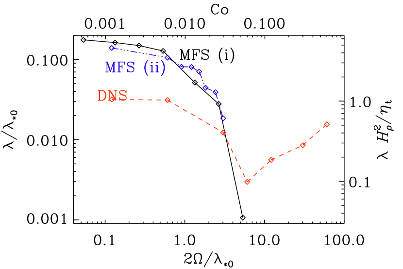
Figure 24: Corrected version of Fig. 2 of Losada et al. (2013) showing the dependence of $\lambda/\lambda_{\ast 0}$ on $2\Omega/\lambda_{\ast 0}$ for DNS (red dashed line), compared with MFS (i) where $q_{\rm p0}=20$ and $\beta_{\rm p}=0.167$ (black solid line), and MFS (ii) where $q_{\rm p0}=32$ and $\beta_{\rm p}=0.058$ (blue dash-dotted line).