Decoherence in neutrino propagation through matter, and bounds from IceCube/DeepCore

Abstract

We revisit neutrino oscillations in matter considering the open quantum system framework, which allows to introduce possible decoherence effects generated by New Physics in a phenomenological manner. We assume that the decoherence parameters $\gamma_{ij}$ may depend on the neutrino energy, as $\gamma_{ij}=\gamma_{ij}^{0}(E/\text{GeV})^{n}$ $(n=0,\pm 1,\pm 2)$. The case of non-uniform matter is studied in detail and, in particular, we develop a consistent formalism to study the non-adiabatic case dividing the matter profile into an arbitrary number of layers of constant densities. This formalism is then applied to explore the sensitivity of IceCube and DeepCore to this type of effects. Our study is the first atmospheric neutrino analysis where a consistent treatment of the matter effects in the three-neutrino case is performed in presence of decoherence. We show that matter effects are indeed extremely relevant in this context. We find that IceCube is able to considerably improve over current bounds in the solar sector ($\gamma_{21}$) and in the atmospheric sector ($\gamma_{31}$ and $\gamma_{32}$) for $n=0,1,2$ and, in particular, by several orders of magnitude (between 3 and 9) for the $n=1,2$ cases. For $n=0$ we find $\gamma_{32},\gamma_{31}<4.0\cdot 10^{-24}(1.3\cdot 10^{-24})$ GeV and $\gamma_{21}<1.3\cdot 10^{-24}(4.1\cdot 10^{-24})$ GeV at the 95% CL, for normal (inverted) mass ordering.

1 Introduction

The accurate measurement of the mixing angle $\theta_{13}$ by reactor neutrino experiments An:2015rpe , with a small uncertainty comparable to that for $\theta_{12}$, has initiated a precision era for neutrino physics. In the standard three-family framework, the main remaining issues are the possible observation of leptonic CP violation, the determination of the ordering of neutrino masses and probing the Dirac or Majorana nature of neutrinos. Some hints currently exist in the latest data collected by NOvA and T2K which seem to point to maximal CP violation in the neutrino sector, but the statistical significance is still low T2K-2017 ; NOvA-Seminar-FNAL-2017 . Likewise, a global fit to neutrino oscillation data seems to show a mild preference for a normal mass ordering (see for instance nufit ; Esteban:2016qun ), which needs to be confirmed as more data become available.

At the same time, and in view of the precision of present and near future neutrino facilities, it is of key importance to verify if neutrinos have unexpected properties caused by New Physics (NP) beyond the standard three-family framework. In this work we study one of the possible windows to NP, the so-called quantum decoherence in neutrino oscillations, and update the existing bounds by analyzing IceCube and DeepCore data on atmospheric neutrinos. In particular, we are interested in a kind of decoherence effects in neutrino oscillations studied, for example, in Benatti:2000ph ; Lisi:2000zt ; Gago:2000qc ; Gago:2002na ; Morgan:2004vv ; Hooper:2004xr ; Fogli:2007tx ; Farzan:2008zv and, more recently, in Bakhti:2015dca ; Gomes:2016ixi ; Oliveira:2016asf ; Coelho:2017zes ; Coelho:2017byq ; Carpio:2017nui . These decoherence effects differ from the standard decoherence caused by the separation of wave packets (see e.g. Giunti:1997wq ; An:2016pvi ) and might arise, instead, from quantum gravity effects Hawking:1976ra ; Ellis:1983jz ; Giddings:1988cx . Throughout this work, for brevity, we will refer to such non-standard decoherence simply as decoherence.

The authors of ref. Lisi:2000zt derived some of the strongest available constraints on neutrino decoherence in neutrino oscillations up to date, using atmospheric neutrino data from the Super-Kamiokande (SK) experiment Fukuda:1998mi ; Fukuda:1998tw ; Fukuda:1998ub ; Fukuda:1998ah . Moreover, they considered the general case in which the decoherence parameters could depend on the neutrino energy via a power law, $\gamma=\gamma_{0}(E/\text{GeV})^{n}$, where $n=0,-1,2$. Nevertheless, these limits were obtained within a simplified two-family framework and without taking into account the matter effects in the neutrino propagation. Furthermore, only a reduced subset of SK data (taken, in fact, almost 20 years ago now) was analyzed Fukuda:1998mi ; Fukuda:1998tw ; Fukuda:1998ub ; Fukuda:1998ah .

In this work, we show that performing a three-flavour analysis which includes the matter effects is essential in order to correctly interpret such constraints. In particular, it is not obvious to which $\gamma_{ij}$ parameter the SK bounds derived in two families Lisi:2000zt would actually apply. We will show that it strongly depends on the neutrino mass ordering and on whether the sensitivity is dominated by the neutrino or antineutrino channels: for neutrinos the decoherence effects at high energies are mainly driven by $\gamma_{21}$ ($\gamma_{31}$) for normal (inverted) ordering, while in the antineutrino channel they are essentially controlled by $\gamma_{32}$ ($\gamma_{21}$) for normal (inverted) ordering. Concerning the solar sector, the authors of ref. Gomes:2016ixi obtained strong constraints on $\gamma_{21}$ from an analysis of KamLAND data Eguchi:2002dm ; Abe:2008aa , for $n=0,\pm 1$. Finally, the authors of ref. deOliveira:2013dia derived several bounds on the atmospheric decoherence parameters $\gamma_{32}$ and $\gamma_{31}$ from an analysis of MINOS data Adamson:2011fa ; Adamson:2011ig ; Adamson:2012rm .

Non-standard decoherence has been invoked several times in the literature in order to decrease the tension in the parameter space among different sets of neutrino oscillation data. For example, in refs. Farzan:2008zv ; Bakhti:2015dca a solution to the LSND anomaly based on quantum decoherence, compatible with global neutrino oscillation data, was proposed. More recently, in Coelho:2017zes it was shown that the $\sim 2\sigma$ tension between T2K and NOvA on the measurement of the atmospheric mixing angle $\theta_{23}$ could be alleviated through the inclusion of decoherence effects in the atmospheric neutrino sector, namely, $\gamma_{23}=(2.3\pm 1.1)\cdot 10^{-23}$ GeV. Such value of $\gamma_{23}$ would be close to the SK bound from ref. Lisi:2000zt , $\gamma<3.5\cdot 10^{-23}$ GeV ($90\%$ CL), but still allowed. This topic has recently brought the attention of a part of the community. In fact, several analyses of decoherence effects on present and future long-baseline neutrino oscillation experiments have been recently performed (albeit at the probability level only), see e.g. refs. Oliveira:2016asf ; Coelho:2017byq ; Carpio:2017nui . In this work we will show that the reference value for $\gamma_{23}$ considered in Coelho:2017zes is indeed already excluded by IceCube data (we note however that, according to the latest results reported by NOvA, the significance of the tension has been reduced to less than 1$\sigma$ NOvA-Seminar-FNAL-2017 ). Moreover, we find that IceCube and DeepCore data are able to improve significantly over most of the constraints in past literature, both for solar and atmospheric decoherence parameters, in some cases by several orders of magnitude.

The paper is structured as follows. In sec. 2 we present the formalism and discuss the effects of decoherence on the oscillation probabilities. We first review the case of constant matter density profile, and then proceed to discuss the case of non-uniform matter. In particular we show that, within the adiabatic approximation, no significant bounds on the decoherence parameters can be extracted from solar neutrino data when the neutrino energy is assumed to be conserved. We then proceed to develop a formalism which permits a consistent treatment of the decoherence effects on neutrino propagation in non-uniform matter when the adiabaticity condition is not fulfilled, as is the case of atmospheric neutrino experiments. In sec. 3 we apply this formalism to the computation of the relevant oscillation probabilities in the atmospheric neutrino case, discussing the main features arising in presence of decoherence. Section 4 summarizes the main features of the IceCube and DeepCore experiments, the data sets considered in our analysis, and the details of our numerical simulations. Our results are then presented and discussed in sec. 5. Finally, we summarize and draw our conclusions in sec. 6. A and B discuss technical details regarding some of the approximations used in our numerical calculations.

2 Quantum decoherence: Density matrix formalism

The evolution of the density matrix $\rho$ in the neutrino system can be described as

$$\frac{d\rho}{dt}=-i\left[H,\rho\right]-\mathcal{D}\left[\rho\right],$$ (1)

where $H$ is the Hamiltonian of the neutrino system and the second term $\mathcal{D}\left[\rho\right]$ parameterizes the decoherence effects. In vacuum, the diagonal elements of the Hamiltonian are given by $h_{i}=m_{i}^{2}/(2E)$, where $m_{i}\ (i=1,2,3)$ are the masses of the three neutrinos and $E$ is the neutrino energy. Here $\rho$ is defined in the flavour basis, with matrix elements $\rho_{\alpha\beta}$. Throughout this work, we will use Greek indices for flavor ($\alpha,\beta=e,\mu,\tau$), and Latin indices for mass eigenstates ($i,j=1,2,3$).

A notable simplification of eq. (1) can be achieved via the following set of assumptions. First, assuming complete positivity, the decoherence term $\mathcal{D}\left[\rho\right]$ can be written in the so-called Lindblad form Lindblad:1975ef ; Banks:1983by

$$\mathcal{D}\left[\rho\right]=\sum_{m}\left[\left\{\rho,D_{m}D_{m}^{\dagger}\right\}-2D_{m}\rho D_{m}^{\dagger}\right],$$ (2)

where $D_{m}$ is a general complex matrix. Second, avoiding unitarity violation, which is equivalent to imposing the condition $d\,\text{Tr}[\rho]/dt=0$, requires $D_{m}$ to be Hermitian. Moreover, $D_{m}=D_{m}^{\dagger}$ implies that the entropy $S=\text{Tr}[\rho\,\ln\rho]$ increases with time. Finally, a key assumption is the average energy conservation of the neutrino system, which is satisfied when

$$[H,D_{m}]=0.$$ (3)

In presence of matter effects, the Hamiltonian is diagonalized by the unitary mixing matrix $\tilde{U}$ (throughout this paper, in our notation the presence of a tilde denotes that a quantity is affected by matter effects). Therefore, after imposing the energy conservation condition given by eq. (3), we get

$$\begin{array}[]{rcl}H&=&\tilde{U}\,\text{diag}\left\{\tilde{h}_{1},\tilde{h}_{2},\tilde{h}_{3}\right\}\tilde{U}^{\dagger}\equiv\tilde{U}H_{d}\tilde{U}^{\dagger},\\ D_{m}&=&\tilde{U}\,\text{diag}\left\{d_{m}^{1},d_{m}^{2},d_{m}^{3}\right\}\tilde{U}^{\dagger}\equiv\tilde{U}D_{m}^{d}\tilde{U}^{\dagger}.\end{array}$$ (4)

This implies that the average energy is conserved along the whole neutrino propagation (through vacuum and matter). This assumption is indeed crucial for our analysis. It is expected to be fulfilled in vacuum and in very good approximation in matter. While we assume that the quantum decoherence itself does not cause the violation of energy conservation, due to the standard neutrino interaction with matter, for large neutrino energies the energy is not exactly conserved in presence of matter due to a small energy transfer to the background fermions. Therefore, in this case, eq. (4) does not hold exactly. This issue has been analyzed in detail in Oliveira:2014jsa ; Oliveira:2016asf ; Carpio:2017nui , where it was shown that in a more general framework in which energy conservation is not assumed, two types of effects in the neutrino oscillation probabilities can essentially be distinguished: pure decoherence effects which suppress the oscillating terms, and the so called relaxation effects which affect non-oscillating terms. In Morgan:2004vv ; Oliveira:2014jsa it was shown that, for atmospheric neutrino oscillations, the relaxation effects which arise when the energy is not conserved are proportional to $\cos^{2}2\theta_{23}$. This suppresses relaxation effects with respect to pure decoherence effects by at least two orders of magnitude, since $\cos^{2}2\theta_{23}$ is currently constrained by experimental data at the level $\cos^{2}2\theta_{23}<0.034$ at 95% CL nufit ; Esteban:2016qun . We will thus focus on the analysis of pure decoherence effects in atmospheric neutrino oscillations assuming that the neutrino energy is conserved, and therefore eq. (4) satisfied, along the whole propagation.

From a model-independent point of view, the $d_{m}^{j}$ are free parameters that could a priori depend on the matter effects. However, the most common assumption in the literature is to assume that the $d_{m}^{j}$ are independent of the matter density even in presence of matter effects.. In order to be consistent with most previous studies and to compare the bounds obtained in our analysis with the constraints derived in previous publications, we will also assume that this is the case. Notice that this assumption does not imply that the matter effects are not relevant when neutrino propagation is affected by decoherence: it just implies that the $d_{m}^{j}$ are assumed to be constant during neutrino propagation through the Earth.

2.1 Neutrino propagation in uniform matter

Performing the following change of basis

$$\tilde{\rho}=\tilde{U}^{\dagger}\rho\tilde{U},$$ (5)

eq. (1) can be rewritten as

$$\frac{d\tilde{\rho}}{dt} =-i\left[H_{d},\tilde{\rho}\right]-\sum_{m}\left[\left\{\tilde{\rho},(D_{m}^{d})^{2}\right\}-2D_{m}^{d}\,\tilde{\rho}\,D_{m}^{d}\right]$$

$$-\tilde{U}^{\dagger}\frac{d\tilde{U}}{dt}\tilde{\rho}-\tilde{\rho}\frac{d\tilde{U}^{\dagger}}{dt}\tilde{U}.$$ (6)

If the matter profile is constant along the neutrino path, the system of equations becomes diagonal in $\tilde{\rho}_{ij}$

$$\frac{d\tilde{\rho}_{ij}}{dt}=-\left[\gamma_{ij}-i\Delta\tilde{h}_{ij}\right]\tilde{\rho}_{ij},$$ (7)

where we have defined

$$\gamma_{ij}\equiv\sum_{m}\left(d_{m}^{i}-d_{m}^{j}\right)^{2}=\gamma_{ji}>0\,;\;\;\;\;\;\;\;\Delta\tilde{h}_{ij}=\tilde{h}_{i}-\tilde{h}_{j}.$$ (8)

Therefore, the solution of eq. (1) for constant matter is simply given by

$$\rho_{\alpha\beta}(t)=\left[\tilde{U}\tilde{\rho}(t)\tilde{U}^{\dagger}\right]_{\alpha\beta},$$ (9)

with

$$\tilde{\rho}_{ij}(t)=\tilde{\rho}_{ij}(0)\,e^{-\left[\gamma_{ij}-i\Delta\tilde{h}_{ij}\right]t},$$ (10)

where $\tilde{\rho}_{ij}(0)$ is determined by the initial conditions of the system. For instance, if the source produces only neutrinos of flavor $\alpha$, the initial conditions are given by

$$\tilde{\rho}_{ij}(0)=\tilde{U}^{*}_{\alpha i}\tilde{U}_{\alpha j}\,.$$ (11)

As a result, the oscillation probabilities in presence of decoherence (for a constant matter profile) read

$$P_{\alpha\beta} \equiv P(\nu_{\alpha}\to\nu_{\beta})=\text{Tr}\left[\hat{\rho}^{(\alpha)}(t)\hat{\rho}^{(\beta)}(0)\right]$$

$$=\text{Tr}\left[\hat{\rho}^{(\alpha)}(t)|\nu_{\beta}\rangle\langle\nu_{\beta}|\right]=\langle\nu_{\beta}|\hat{\rho}^{(\alpha)}(t)|\nu_{\beta}\rangle$$

$$=\sum_{i,j}\tilde{U}_{\beta i}\tilde{U}^{*}_{\beta j}\,\tilde{\rho}_{ij}(t)$$

$$=\sum_{i,j}\tilde{U}^{*}_{\alpha i}\tilde{U}_{\beta i}\tilde{U}_{\alpha j}\tilde{U}^{*}_{\beta j}e^{-\left[\gamma_{ij}-i\Delta\tilde{h}_{ij}\right]t}\,,$$ (12)

where $\hat{\rho}$ denotes the density operator. Finally, after some manipulation the above equation can be rewritten in the more familiar form

$$P_{\alpha\beta} =\delta_{\alpha\beta}-2\sum_{i<j}{\rm Re}\left[\tilde{U}_{\alpha i}^{*}\tilde{U}_{\beta i}\tilde{U}_{\alpha j}\tilde{U}_{\beta j}^{*}\right]\left(1-e^{-\gamma_{ij}L}\cos\tilde{\Delta}_{ij}\right)$$

$$-2\sum_{i<j}{\rm Im}\left[\tilde{U}_{\alpha i}^{*}\tilde{U}_{\beta i}\tilde{U}_{\alpha j}\tilde{U}_{\beta j}^{*}\right]e^{-\gamma_{ij}L}\sin\tilde{\Delta}_{ij},$$ (13)

with

$$\tilde{\Delta}_{ij}\equiv\frac{\Delta\tilde{m}^{2}_{ij}L}{2E},\;\;\;\;\;\;\;\;\;\;\gamma_{ij}=\gamma_{ji}\equiv\gamma_{ij}^{0}\left(\frac{E}{\text{GeV}}\right)^{n},$$ (14)

where $\Delta\tilde{m}^{2}_{ij}\equiv\tilde{m}^{2}_{i}-\tilde{m}^{2}_{j}$ are the effective mass squared differences of neutrinos in matter and we have used the approximation $L\approx t$, $L$ being the distance traveled by the neutrino as it propagates. Note that the power-law dependence on the neutrino energy given by eq. (14) breaks Lorentz invariance, except for the case with $n=-1$ which gives similar effects to the neutrino decay (see e.g. GonzalezGarcia:2008ru ). However, the effect encoded in $\gamma_{ij}$ only suppresses the oscillatory terms in the oscillation probability while a neutrino decay would also affect the non-oscillatory terms. Therefore, in the framework considered in this work the total sum of the probabilities adds up to $1$, while this is not the case for neutrino decay.

From eqs. (13) and (14), one would expect to have a sizable effect in neutrino oscillations for $\gamma_{ij}L\sim 1$. This condition gives an estimate of the values of $\gamma_{ij}$ for which an effect may be experimentally observable:

$$\gamma_{ij}^{0}\sim 1.7\cdot 10^{-19}\left(\frac{L}{\text{km}}\right)^{-1}\left(\frac{E}{\text{GeV}}\right)^{-n}\ \text{GeV}.$$ (15)

Nevertheless, we would like to remark that fulfilling this condition is not enough to have sensitivity to decoherence effects, as we will discuss in the next subsection.

Even though in our simulations we will numerically compute the exact oscillation probabilities, in order to understand qualitatively the impact of decoherence on the oscillation pattern it is useful to derive approximate analytical expressions. In this work, we will be focusing on the study of atmospheric neutrino oscillations, for which the oscillation channel $P_{\mu\mu}$ is most relevant. Recently, in Denton:2016wmg ; Denton:2018hal approximated but very accurate analytical expressions for the standard oscillation probabilities in presence of constant matter density were derived. For the $\nu_{\mu}\to\nu_{\mu}$ oscillation channel including decoherence effects, using the same parametrization as in ref. Denton:2018hal , we find:

$$P_{\mu\mu} =1-A_{21}\left[1-e^{-\gamma_{21}L}\cos\tilde{\Delta}_{21}\right]-A_{32}\left[1-e^{-\gamma_{32}L}\cos\tilde{\Delta}_{32}\right]$$

$$-A_{31}\left[1-e^{-\gamma_{31}L}\cos\tilde{\Delta}_{31}\right],$$ (16)

where

$$A_{ij} \equiv A_{ij}(\theta_{23},\tilde{\theta}_{12},\tilde{\theta}_{13},\delta)$$

$$=2|U_{\mu i}(\theta_{23},\tilde{\theta}_{12},\tilde{\theta}_{13},\delta)|^{2}|U_{\mu j}(\theta_{23},\tilde{\theta}_{12},\tilde{\theta}_{13},\delta)|^{2},$$ (17)

and the effective mass splittings and mixing angles in matter can be expressed as Denton:2018hal :

$$\cos 2\tilde{\theta}_{13} =\frac{\cos 2\theta_{13}-a/\Delta m^{2}_{ee}}{\sqrt{(\cos 2\theta_{13}-a/\Delta m^{2}_{ee})^{2}+\sin^{2}2\theta_{13}}},$$

$$\cos 2\tilde{\theta}_{12} =\frac{\cos 2\theta_{12}-a^{\prime}/\Delta m^{2}_{21}}{\sqrt{(\cos 2\theta_{12}-a^{\prime}/\Delta m^{2}_{21})^{2}+\sin^{2}2\theta_{12}\cos^{2}(\tilde{\theta}_{13}-\theta_{13})}},$$

$$\Delta\tilde{m}^{2}_{21} =\Delta m^{2}_{21}\sqrt{(\cos 2\theta_{12}-a^{\prime}/\Delta m^{2}_{21})^{2}+\sin^{2}2\theta_{12}\cos^{2}(\tilde{\theta}_{13}-\theta_{13})},$$

$$\Delta\tilde{m}^{2}_{31} =\Delta m^{2}_{31}+(a-\frac{3}{2}a^{\prime})+\frac{1}{2}(\Delta\tilde{m}^{2}_{21}-\Delta m^{2}_{21}),$$

$$\Delta\tilde{m}^{2}_{32} =\Delta\tilde{m}^{2}_{31}-\Delta\tilde{m}^{2}_{21}.$$ (18)

Here, $a\equiv 2\sqrt{2}G_{F}n_{e}E$, where $G_{F}$ is the Fermi constant and $n_{e}$ is the electron number density along the neutrino path, $\Delta m^{2}_{ee}\equiv\cos^{2}\theta_{12}\Delta m^{2}_{31}+\sin^{2}\theta_{12}\Delta m^{2}_{32}$, and $a^{\prime}=a\cos^{2}\tilde{\theta}_{13}+\Delta m^{2}_{ee}\sin^{2}(\tilde{\theta}_{13}-\theta_{13})$. The corresponding probability for antineutrinos is obtained simply replacing $a\to-a$ and $\delta\to-\delta$, where $\delta$ denotes the Dirac CP phase.

2.2 Neutrino propagation in non-uniform matter: adiabatic regime

Equation (13) applies for constant density profiles (which is a very good approximation in the case of long-baseline neutrino oscillation experiments such as T2K or NOvA), but if the matter density is not constant the analysis becomes more complicated. Nevertheless, when the adiabaticity condition ${d\tilde{U}}/{dt}\ll 1$ is fulfilled, as in the solar neutrino case, the solution of the evolution equations given by eqs. (9) and (10) is still a good approximation. In such a case, the oscillation probability is given by

$$P_{\alpha\beta} =\langle\nu_{\beta}|\hat{\rho}^{(\alpha)}(t)|\nu_{\beta}\rangle$$

$$=\sum_{i,j}\tilde{\rho}^{(\alpha)}_{ij}(0)e^{-\left[\gamma_{ij}-i\Delta\tilde{h}_{ij}\right]t}\langle\nu_{\beta}|\tilde{\nu}_{i}^{eff}\rangle\langle\tilde{\nu}_{j}^{eff}|\nu_{\beta}\rangle,$$ (19)

where $\nu_{i}^{eff}$ denotes the effective mass eigenstates at time $t$. In the case of solar neutrinos, the initial flux of $\nu_{e}$ is produced in the solar core and the initial conditions are given by:

$$\tilde{\rho}^{(e)}_{ij}(0)=\tilde{U}_{ei}^{0*}\tilde{U}_{ej}^{0},$$ (20)

where $\tilde{U}^{0}$ denotes the effective mixing matrix at the production point. On the other hand, since the evolution is adiabatic, when the neutrinos come out from the Sun we have $|\tilde{\nu}_{i}^{eff}\rangle=|\nu_{i}\rangle$ and thus

$$P_{e\beta} \approx\sum_{i,j}\tilde{U}_{ei}^{0*}U_{\beta i}\tilde{U}^{0}_{ej}U_{\beta j}^{*}e^{-\left[\gamma_{ij}-i\Delta\tilde{h}_{ij}\right]t}$$

$$=\sum_{i}|\tilde{U}_{ei}^{0}|^{2}|U_{\beta i}|^{2}$$

$$+2\sum_{i<j}{\rm Re}\left[\tilde{U}_{ei}^{0*}U_{\beta i}\tilde{U}_{ej}^{0}U_{\beta j}^{*}\right]e^{-\gamma_{ij}t}\cos\tilde{\Delta}_{ij}$$

$$-2\sum_{i<j}{\rm Im}\left[\tilde{U}_{ei}^{0*}U_{\beta i}\tilde{U}_{ej}^{0}U_{\beta j}^{*}\right]e^{-\gamma_{ij}t}\sin\tilde{\Delta}_{ij}.$$ (21)

Finally, for solar neutrinos observed at the Earth we obtain, after averaging over the oscillating phase:

$$P_{e\beta}\approx\sum_{i}|\tilde{U}_{ei}^{0}|^{2}|U_{\beta i}|^{2},$$ (22)

which coincides with the standard result. In other words, the decoherence effects encoded in $\gamma_{ij}$ can not be bounded by solar neutrino oscillation experiments. This is due to the standard loss of coherence in the propagation from the Sun to the Earth, which strongly suppresses the oscillating terms. In a similar fashion high-energy astrophysical neutrinos at IceCube are not sensitive to decoherence either, since these neutrinos are produced in distant astrophysical sources and thus the oscillations will have averaged out by the time they reach the detector.

2.3 Neutrino propagation in non-uniform matter: layers of constant density

In the atmospheric neutrino case, the matter profile cannot be considered constant since the neutrinos propagate through the Earth crust, mantle and core, which have different densities. The adiabaticity condition is not fulfilled either. In this case, eq. (6) should be solved including the non-adiabatic terms, which give non-diagonal contributions. Even though this can be done numerically, we will show that dividing the matter profile into layers of constant density considerably simplifies the analysis and reduces the computational complexity of the problem. In particular, this is crucial in the case of atmospheric neutrino oscillation experiments, for which numerical studies are already computationally demanding even in the standard three-family scenario. Dividing the matter profile into layers of different constant densities has proved to be a very good approximation in the standard three-family scenario and, therefore, we expect the same level of accuracy in presence of decoherence. Since the matter is constant in each layer, the evolution equations can be solved for each layer $M$ as in sec. 2.1:

$$\rho_{\alpha\beta}^{M}(t_{M}) =\left[\tilde{U}^{M}\tilde{\rho}^{M}(t_{M})(\tilde{U}^{M})^{\dagger}\right]_{\alpha\beta},$$

$$\tilde{\rho}^{M}_{ij}(t_{M}) =\tilde{\rho}^{M}_{ij}(t_{M,0})\,e^{-\left[\gamma_{ij}-i\Delta\tilde{h}^{M}_{ij}\right]\Delta t_{M}},$$ (23)

where $\Delta t_{M}\equiv t_{M}-t_{M,0}$, and $t_{M,0}$ and $t_{M}$ denote the initial and final times for the propagation along layer $M$, respectively. Now the problem of computing the probability is just reduced to performing properly the matching among the evolution on the different layers. Let us first consider the simplest case of two layers $A$ and $B$. The oscillation probability when the neutrino exits the second layer (at time $t_{B}$) is given by

$$P_{\alpha\beta}=\langle\nu_{\beta}|\hat{\rho}^{(\alpha)}(t_{B})|\nu_{\beta}\rangle=\sum_{i,j}\tilde{U}^{B}_{\beta i}\,\tilde{U}^{B*}_{\beta j}\,\tilde{\rho}^{B}_{ij}(t_{B,0})\,e^{-\left[\gamma_{ij}-i\Delta\tilde{h}^{B}_{ij}\right]\Delta t_{B}}\,.$$ (24)

The key point here is that the matching should be done between the solutions of eq. (1) at the frontier between the two layers and in the flavor basis, as

$$\rho^{A}_{\alpha\beta}(t_{A})=\rho^{B}_{\alpha\beta}(t_{B,0}).$$ (25)

After imposing the matching condition, the elements of the density matrix in the second layer at $t_{B,0}$ can be written in the matter basis as:

$$\tilde{\rho}^{B}_{ij}(t_{B,0}) =\left[(\tilde{U}^{B})^{\dagger}\tilde{U}^{A}\tilde{\rho}^{A}(t_{A})(\tilde{U}^{A})^{\dagger}\tilde{U}^{B}\right]_{ij}$$

$$=\tilde{U}^{B*}_{\delta i}\tilde{U}^{A}_{\delta l}\tilde{\rho}^{A}_{ln}(t_{A,0})e^{-\left[\gamma_{ln}-i\Delta\tilde{h}^{A}_{ln}\right]\Delta t_{A}}\tilde{U}^{A*}_{\gamma n}\tilde{U}^{B}_{\gamma j}$$

$$=\tilde{U}^{B*}_{\delta i}\tilde{U}^{A}_{\delta l}\tilde{U}^{A*}_{\alpha l}\tilde{U}^{A}_{\alpha n}e^{-\left[\gamma_{ln}-i\Delta\tilde{h}^{A}_{ln}\right]\Delta t_{A}}\tilde{U}^{A*}_{\gamma n}\tilde{U}^{B}_{\gamma j},$$ (26)

where we have considered that the initial flux is made of $\nu_{\alpha}$ as initial condition for the first layer. After substituting this result into eq. (24) we finally obtain

$$P_{\alpha\beta} =\sum_{\delta,\gamma,i,j,l,n}\tilde{U}^{B}_{\beta i}\tilde{U}^{B*}_{\delta i}\tilde{U}^{B}_{\gamma j}\tilde{U}^{B*}_{\beta j}e^{-\left[\gamma_{ij}-i\Delta\tilde{h}^{B}_{ij}\right]\Delta t_{B}}$$

$$\times\tilde{U}^{A}_{\delta l}\tilde{U}^{A*}_{\alpha l}\tilde{U}^{A}_{\alpha n}\tilde{U}^{A*}_{\gamma n}e^{-\left[\gamma_{ln}-i\Delta\tilde{h}^{A}_{ln}\right]\Delta t_{A}}\,.$$ (27)

It can be easily checked that, in the limit $\gamma_{ij}\rightarrow 0$, the standard oscillation probability is recovered. In the three-layer case, following the same procedure we find

$$P_{\alpha\beta} =\sum_{\delta,\gamma,\theta,\phi,i,j,l,n,m,k}\tilde{U}^{C}_{\beta i}\tilde{U}^{C*}_{\delta i}\tilde{U}^{C}_{\gamma j}\tilde{U}^{C*}_{\beta j}e^{-\left[\gamma_{ij}-i\Delta\tilde{h}^{C}_{ij}\right]\Delta t_{C}}$$

$$\times\tilde{U}^{B}_{\delta l}\tilde{U}^{B*}_{\theta l}\tilde{U}^{B}_{\phi n}\tilde{U}^{B*}_{\gamma n}e^{-\left[\gamma_{ln}-i\Delta\tilde{h}^{B}_{ln}\right]\Delta t_{B}}$$

$$\times\tilde{U}^{A}_{\theta m}\tilde{U}^{A*}_{\alpha m}\tilde{U}^{A}_{\alpha k}\tilde{U}^{A*}_{\phi k}e^{-\left[\gamma_{mk}-i\Delta\tilde{h}^{A}_{mk}\right]\Delta t_{A}}.$$ (28)

The procedure can be easily generalized to an arbitrary number of layers. Indeed, under the approximation $L\approx t$, and defining

$$\tilde{\mathcal{A}}^{M}_{\alpha\beta\gamma\delta}\equiv\sum_{i,j}\tilde{U}^{M}_{\alpha i}\tilde{U}^{M*}_{\beta i}\tilde{U}^{M}_{\gamma j}\tilde{U}^{M*}_{\delta j}e^{-\left[\gamma_{ij}-i(\Delta\tilde{m}^{M}_{ij})^{2}/2E\right]\Delta L_{M}},$$ (29)

the probabilities can be written in a more compact way as for two layers

$$P_{\alpha\beta}=\sum_{\delta,\gamma}\tilde{\mathcal{A}}^{B}_{\beta\delta\gamma\beta}\tilde{\mathcal{A}}^{A}_{\delta\alpha\alpha\gamma},$$ (30)

for three layers

$$P_{\alpha\beta}=\sum_{\delta,\gamma,\theta,\phi}\tilde{\mathcal{A}}^{C}_{\beta\delta\gamma\beta}\tilde{\mathcal{A}}^{B}_{\delta\theta\phi\gamma}\tilde{\mathcal{A}}^{A}_{\theta\alpha\alpha\phi},$$ (31)

for N layers

$$P_{\alpha\beta}=\sum_{\delta,\gamma,\theta,\phi,...,\xi,\omega,\varphi,\rho}\tilde{\mathcal{A}}^{N}_{\beta\delta\gamma\beta}\tilde{\mathcal{A}}^{N-1}_{\delta\theta\phi\gamma}...\;\tilde{\mathcal{A}}^{B}_{\xi\varphi\rho\omega}\tilde{\mathcal{A}}^{A}_{\varphi\alpha\alpha\rho}\phantom{mmmm}.$$ (32)

3 Atmospheric oscillation probabilities with decoherence

Atmospheric neutrino oscillations take place in a regime where matter effects are significant and can even dominate the oscillations. The relevance of matter effect increases with neutrino energy and is very different for neutrinos and antineutrinos, as the sign of the matter potential changes between the two cases. Matter effects also depend strongly on the neutrino mass ordering. In order to understand better the numerical results shown in this paper, it is useful to derive approximate expressions for the oscillations in the $\nu_{\mu}\to\nu_{\mu}$ and $\bar{\nu}_{\mu}\to\bar{\nu}_{\mu}$ channels in the presence of strong matter effects.

From the results obtained in refs. Denton:2016wmg ; Denton:2018hal , for neutrino energies $E\raise 1.29167pt\hbox{$\;>$\kern-7.5pt\raise-4.73611pt\hbox{$\sim\;$}}15$ GeV matter effects drive the effective mixing angles in matter $\tilde{\theta}_{12}$ and $\tilde{\theta}_{13}$ to either 0 or $\pi/2$, depending on the channel (neutrino/antineutrino) and the mass ordering. It is easy to show that, in this regime, the oscillation probabilities in eq. (2.1) can be approximated as:

$$P^{\mathrm{NO}}_{\mu\mu}\approx 1-\frac{1}{2}\sin^{2}2\theta_{23}\left(1-e^{-\gamma_{21}L}\cos\tilde{\Delta}_{21}\right)$$ (33)

for neutrinos, and

$$P^{\mathrm{NO}}_{\bar{\mu}\bar{\mu}}\approx 1-\frac{1}{2}\sin^{2}2\theta_{23}\left(1-e^{-\gamma_{32}L}\cos\tilde{\Delta}_{32}\right)$$ (34)

for antieneutrinos, assuming a normal ordering (NO). For inverted ordering (IO) we get instead

$$P^{\mathrm{IO}}_{\mu\mu}\approx 1-\frac{1}{2}\sin^{2}2\theta_{23}\left(1-e^{-\gamma_{31}L}\cos\tilde{\Delta}_{31}\right)$$ (35)

for neutrinos,

$$P^{\mathrm{IO}}_{\bar{\mu}\bar{\mu}}\approx 1-\frac{1}{2}\sin^{2}2\theta_{23}\left(1-e^{-\gamma_{21}L}\cos\tilde{\Delta}_{21}\right)$$ (36)

for antineutrinos. In the limit $\gamma_{ij}=0$, eqs. (33)-(36) reassemble the standard neutrino oscillation probabilities derived under the one-dominant mass-scale approximation Pantaleone:1993di . From eqs. (33)-(36) it is easy to see that the approximated oscillation probabilities for an inverted mass ordering can be obtained from the corresponding ones for normal mass ordering, just performing the following transformation:

$$\gamma_{21},\tilde{\Delta}_{21} \to\gamma_{31},\tilde{\Delta}_{31},$$ (37)

$$\gamma_{32},\tilde{\Delta}_{32} \to\gamma_{21},\tilde{\Delta}_{21}.$$ (38)

Moreover, note that since the three decoherence parameters and the three mass splittings are related (see eqs. (8) and (14)), these two transformations automatically imply that

$$\gamma_{31},\tilde{\Delta}_{31}\to\gamma_{32},\tilde{\Delta}_{32}.$$ (39)

Equations (33)-(36) illustrate why a proper consideration of the matter effects in the context of three families is of key importance in order to correctly interpret the bounds extracted within a simplified two-flavour approximation (as done in e.g. ref. Lisi:2000zt ). According to our analytical results, which will be confirmed numerically below, the constraints obtained from SK in a two-family approximation cannot be simply applied to $\gamma_{31}$ or $\gamma_{32}$, contrary to the naive expectation. In fact, the interpretation of such limits depends strongly on the ordering of neutrino masses and on whether the sensitivity is dominated by the neutrino or antineutrino channels: for neutrinos the decoherence effects at high energies would be mainly driven by $\gamma_{21}$ ($\gamma_{31}$) for normal (inverted) ordering. Conversely, in the antineutrino channel decoherence effects are essentially controlled by $\gamma_{32}$ ($\gamma_{21}$) for normal (inverted) ordering. Therefore, we conclude that in order to avoid any misinterpretation of the bounds from atmospheric neutrinos, a three-family approach including matter effects should be considered.

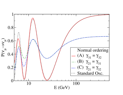
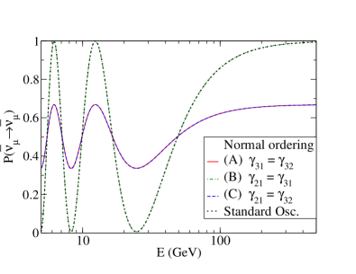
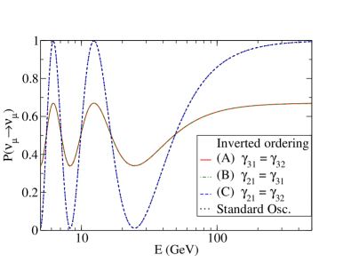
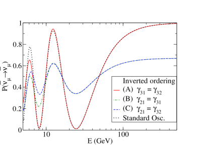
Figure 1: The $\nu_{\mu}\to\nu_{\mu}$ (top panels) and $\overline{\nu}_{\mu}\to\overline{\nu}_{\mu}$ (bottom panels) oscillation probabilities with ($n=0$) and without decoherence effects as a function of the neutrino energy. The probabilities have been computed for normal (left panels) and inverted (right panels) neutrino mass ordering, using a three-layer model for the Earth matter density profile, and correspond to the case in which the neutrinos cross the center of the Earth. In this figure, in the cases where decoherence effects are included we have set the parameters listed in the legend to the same constant value $\gamma=2.3\cdot 10^{-23}$ GeV.

Figure 1 shows the numerically obtained $\nu_{\mu}\to\nu_{\mu}$ (top panels) and $\overline{\nu}_{\mu}\to\overline{\nu}_{\mu}$ (bottom panels) oscillation probabilities for NO (left panels) and IO (right panels), with and without decoherence, as a function of the neutrino energy for a three-layer model (details on the accuracy of our three-layer model and the specific parameters used in our simulations can be found in A). For the sake of simplicity, in this section we focus on the case $n=0$, where the $\gamma_{ij}$ do not depend on the neutrino energy (the results for different values of $n$ show a similar qualitative behavior). The standard oscillation parameters have been fixed to the best-fit values given in nufit ; Esteban:2016qun .

Figure 1 clearly shows how the decoherence tends to damp the oscillatory behavior, in qualitative agreement with eq. (2.1) and the corresponding approximate expressions given by eqs. (33)-(36). Note that eq. (2.1) has been obtained under several approximations and, in particular, considering only one layer with constant matter density. However, we should stress that in our simulations the computation of the probability has been done numerically, considering a three-layer matter profile (see A for details).

Since the three $\gamma_{ij}$ are not completely independent from one another (see eq. (8)), in view of eqs. (33)-(36) and in order to simplify the analysis, hereafter we will distinguish three different representative cases, where the decoherence effects are dominated by just one parameter:

1. Atmospheric limit: $\gamma_{21}=0$ ($\gamma_{32}=\gamma_{31}$),

2. Solar limit I: $\gamma_{32}=0$ ($\gamma_{21}=\gamma_{31}$),

3. Solar limit II: $\gamma_{31}=0$ ($\gamma_{21}=\gamma_{32}$).

In B, we will show that the bounds derived in these limits correspond to the most conservative bounds that can be extracted in the general case. As a reference value for the decoherence parameters, in this section we have considered $\gamma=2.3\cdot 10^{-23}$ GeV, for each of the three limiting cases listed above.

The results in fig. 1 show that, for neutrinos with a NO (top left panel), the impact of decoherence is essentially controlled by $\gamma_{21}$, in good agreement with eq. (33): no significant effects are seen in the atmospheric limit (A), while a similar impact is obtained in the solar limits I (B) and II (C). Conversely, for IO (top right panel) the effects are dominated by $\gamma_{31}$ instead: no effect is observed for the solar limit II (C), while in scenarios (A) and (B) the effect is very similar. This can be qualitatively understood from the approximate probability derived in eq. (35), which only depends on the decoherence parameter $\gamma_{31}$. On the other hand, in the antineutrino case for NO (bottom left panel) no observable decoherence effects take place in case (B), while cases (A) and (C) show a similar behavior, in agreement with eq. (34). Conversely, for IO (bottom right panel) decoherence effects are essentially controlled by $\gamma_{21}$ as shown in eq. (36): therefore, no significant effects are observed in case (A) while a similar impact is obtained for case (B) and (C).

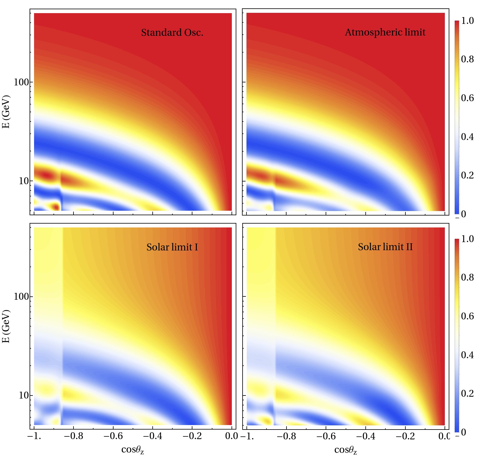
Figure 2: Oscillograms for the neutrino oscillation probability $P_{\mu\mu}$, assuming normal mass ordering. The top left panel corresponds to the case of no decoherence $\gamma_{ij}=0$ whereas the rest of the panels correspond to the three limiting cases mentioned in the text: (A) $\gamma_{32}=\gamma_{31}$ (top right), (B) $\gamma_{31}=\gamma_{21}$ (bottom left) and (C) $\gamma_{32}=\gamma_{21}$ (bottom right). In all cases, the size of the decoherence parameters that are turned on is set to a constant value, $\gamma=2.3\cdot 10^{-23}$ GeV.

Moreover, it should be pointed out that the transformations listed in Eqs. (37)-(39) automatically imply the following equivalence for the results obtained in the three limiting cases listed above:

$$({\rm A})^{\rm NO} \longleftrightarrow({\rm C})^{\rm IO},$$

$$({\rm B})^{\rm NO} \longleftrightarrow({\rm A})^{\rm IO},$$ (40)

$$({\rm C})^{\rm NO} \longleftrightarrow({\rm B})^{\rm IO}.$$

This is also confirmed at the numerical level, as it can be easily seen by comparing the different lines shown in the left (NO) and right (IO) panels in fig. 1 for the three limiting cases.

It is also remarkable that, for both normal and inverted mass orderings, even when the standard oscillations turn off (at very high energies), there is still a large effect on the probability due to decoherence effects, that could potentially be tested with neutrino telescopes like IceCube. In particular, for $E\raise 1.29167pt\hbox{$\;>$\kern-7.5pt\raise-4.73611pt\hbox{$\sim\;$}}200$ GeV one can approximate $\cos\tilde{\Delta}_{ij}\approx 1$, $\forall i,j$. Therefore, in the standard case (with $\gamma_{ij}=0$) the last three terms in eq. (2.1) approximately vanish, leading to $P_{\mu\mu}\approx 1$. However, in presence of decoherence those terms will not vanish completely, as $e^{-\gamma_{ij}L}\cos\tilde{\Delta_{ij}}\neq 1$. This leads to a depletion of $P_{\mu\mu}$, which is no longer equal to 1 in this case. The size of the effect will of course depend on the baseline of the experiment. Since at high energies the oscillation probability does no longer depend on the neutrino energy, at oscillation experiments with a fixed baseline the effect may be hindered by the presence of any systematic errors affecting the normalization of the signal event rates. However, at atmospheric experiments this effect can be disentangled from a simple normalization error by comparing the event rates at different nadir angles.

The dependence of the neutrino probabilities with the zenith angle $\theta_{z}$ is illustrated in fig. 2, assuming a normal mass ordering and fixing the standard oscillation parameters to the best-fit values given in nufit ; Esteban:2016qun . The results are shown as a neutrino oscillogram (see for instance Akhmedov:2006hb ), which represents the oscillation probability in the $P_{\mu\mu}$ channel as a function of neutrino energy and zenith angle $\theta_{z}$ (which can be related to the distance traveled by the neutrino). Figure 2 shows the oscillation probability $P_{\mu\mu}$ in the three limiting cases described above, comparing it to the results in the standard scenario ($\gamma_{ij}=0$). As expected, the effects depend on the direction of the incoming neutrino and they are more relevant in the region $-1\lesssim\cos\theta_{z}\lesssim-0.4$, this is, for very long baselines. This was to be expected, since the decoherence effects are driven by $e^{-\gamma_{ij}L}$. In addition, the dependence of the oscillation probability with the zenith angle at very high energies ($E>100$ GeV) is clearly visible in the bottom panels of fig. 2. As we will show in sec. 5, this will lead to an impressive sensitivity for the IceCube setup. Finally, note that the results for inverted ordering show similar features to those in fig. 2, once the mapping in eq. (40) is applied, and are therefore not shown here.

4 IceCube/DeepCore simulation details and data set

The IceCube neutrino telescope, located at the South Pole, is composed of 5160 DOMs (Digital Optical Module) deployed between 1450 m and 2450 m below the ice surface along 86 vertical strings Aartsen:2016nxy . In the inner core of the detector, a subset of these DOMs were deployed deeper than 1750 m and closer to each other than in the rest of IceCube. This subset of strings is called DeepCore. Due to the shorter distance between its DOMs, the neutrino energy threshold in DeepCore ($\sim 5$ GeV) is lower than in IceCube ($\sim 100$ GeV). This allows DeepCore to observe neutrino events in the energy region where atmospheric oscillations take place, see fig. 1, whereas IceCube only observes high-energy atmospheric neutrino events.

As outlined in sec. 2, for high energy astrophysical neutrinos the effect of non-standard decoherence in the probability would be completely erased by the time they reach the detector. Therefore, in this work we will focus on the observation of atmospheric neutrino events at both IceCube and DeepCore, in the energy range $\sim 10$ GeV to $\sim 1$ PeV. In particular, we have used the three-year DeepCore data on atmospheric neutrinos with energies between $\sim 10$ GeV and $\sim 1$ TeV, taken between May 2011 and April 2014 Aartsen:2014yll , and the one-year IceCube data taken between 2011-2012 TheIceCube:2016oqi ; Jones:2015 ; Arguelles:2015 , corresponding to neutrinos with energies between 200 GeV and 1 PeV.

At IceCube and DeepCore, events are divided according to their topology into “tracks” and “cascades” YanezGarza:2014jia . Tracks are produced by the Cherenkov radiation of muons propagating in the ice. In atmospheric neutrino experiments, muons are typically produced by two main mechanisms: (1) via charged-current (CC) interactions of $\nu_{\mu}$ with nuclei in the detector, and (2) as decay products of mesons (typically pions and kaons) originated when cosmic rays hit the atmosphere. Conversely, cascades are created in CC interactions of $\nu_{e}$ or $\nu_{\tau}$: in this case, the rapid energy loss of electrons as they move through the ice is the origin of an electromagnetic shower. At IceCube/DeepCore, cascades are also observed as the product of hadronic showers generated in neutral-current (NC) interactions for neutrinos of all flavors. Our analysis considers only track-like events observed at both IceCube and DeepCore although, as we will see, some small contamination from cascade events can be expected (especially at low energies).

4.1 IceCube simulation details

For IceCube, the observed event rates are provided in a grid of $10\times 21$ bins Jones:2015 , using 10 bins for the reconstructed energy (logarithmically spaced, ranging from 400 GeV to 20 TeV), and 21 bins for the reconstructed neutrino direction (linearly spaced, between $\cos\theta_{z}^{rec}=-1.02$ and $\cos\theta_{z}^{rec}=0.24$). The muon energy is reconstructed with an energy resolution $\sigma_{\text{log}_{10}(E_{\mu}/\text{GeV})}\sim 0.5$ TheIceCube:2016oqi , while the zenith angle resolution is in the range $\sigma_{\cos\theta_{z}}\in[0.005,0.015]$, depending on the scattering muon angle.

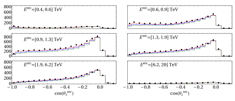
Figure 3: Event distributions obtained for IceCube in our numerical simulations as a function of the reconstructed value of the cosine of the zenith angle, for neutrinos in different reconstructed energy ranges. The lines have been obtained assuming a normal mass ordering, for the following values for the decoherence parameters: $\gamma_{21}=\gamma_{31}=2.3\cdot 10^{-23}$ GeV (solid blue line), $\gamma_{21}=\gamma_{31}=10^{-22}$ GeV (dot-dashed green line) and without decoherence (dashed red line). The observed data points Jones:2015 are represented by the black dots, and the error bars indicate the statistical uncertainties for each bin.

The number of events in each bin is computed as:

$$N_{i}(E^{rec},\theta_{z}^{rec})= \sum_{\pm}\int dE\;d\cos\theta_{z}\,\phi^{\text{atm}}_{\mu,\pm}(E,\theta_{z})P_{\mu\mu}^{\pm}(E,\theta_{z})$$

$$A^{\text{eff}}_{i,\pm,\mu}(E,\theta_{z},E^{rec},\theta_{z}^{rec})e^{-X(\theta_{z})\sigma^{\pm}(E)},$$ (41)

where $E,\theta_{z}$ denote the true values of energy and zenith angle, while $E^{rec},\theta_{z}^{rec}$ refer to their reconstructed quantities. Here, $\phi^{\text{atm}}_{\mu,\pm}$ is the atmospheric flux for muon neutrinos (+) and anti-neutrinos (-), $P_{\mu\mu}^{\pm}(E,\theta_{z})$ is the neutrino/antineutrino oscillation probability given by eq. (28), and $A^{\text{eff}}_{i,\pm,\mu}(E,\theta_{z})$ is the effective area encoding the detector response in neutrino energy and direction (which relates true and reconstructed variables), the interaction cross section and a normalization constant, and has been integrated over the whole data taking period. In our IceCube simulations, we have used the unpropagated atmospheric flux (HondaGaisser) provided by the collaboration TheIceCube:2016oqi ; IceCubeweb , and for the effective area we have used the nominal detector response from refs. TheIceCube:2016oqi ; IceCubeweb . On the other hand, the exponential factor takes into account the absorption of the neutrino flux by the Earth, which increases with the neutrino energy. Here, $X(\theta_{z})$ is the column density along the neutrino path and $\sigma^{\pm}(E)$ is the total inclusive cross section for $\nu_{\mu}$ or $\bar{\nu}_{\mu}$. Note that in eq. (4.1) no contamination from cascade events is considered since the mis-identification rate is expected to be negligible at these energies Weaver:2015 . Similarly, the number of atmospheric muons that pass the selection cuts can also be neglected, given the extremely good angular resolution at these energies TheIceCube:2016oqi .

Figure 3 shows the expected number of events for IceCube from our numerical simulations including decoherence, for $\gamma_{21}=\gamma_{31}=2.3\cdot 10^{-23}$ GeV (solid blue lines) and $\gamma_{21}=\gamma_{31}=10^{-22}$ GeV (dot-dashed green lines), as a function of $\cos\theta_{z}^{rec}$, for events in different reconstructed energy ranges. For simplicity, we have considered the $n=0$ case (that is, $\gamma_{ij}$ independent of the neutrino energy). The expected result without decoherence is also shown for comparison (dashed red lines), while the observed data Jones:2015 are shown by the black dots.

For the analysis of the IceCube data we have performed a Poissonian log-likelihood analysis doing a simultaneous fit on the following parameters: $\Delta m^{2}_{32},\,\theta_{23}$ and $\gamma_{ij}$. The rest of the oscillation parameters have been kept fixed to their current best-fit values from ref. nufit ; Esteban:2016qun . The most relevant systematic errors used in the fit are summarized in tab. 1, and have been taken from refs. TheIceCube:2016oqi ; Arguelles:2015 ; IceCubeweb . For each systematic uncertainty a pull term is added to the $\chi^{2}$ following the values listed in the table, except in the cases indicated as “Free” (when the corresponding nuisance parameter is allowed to float freely in the fit).

Table 1: The most relevant systematic errors used in our analysis of IceCube data, taken from refs. TheIceCube:2016oqi ; Arguelles:2015 ; IceCubeweb .

Source of uncertainty	Value
Flux - normalization	Free
Flux - $\pi/K$ ratio	10%
Flux - energy dependence as $(E/E_{0})^{\eta}$	$\Delta\eta=0.05$
Flux - $\bar{\nu}/\nu$	2.5%
DOM efficiency	5%
Photon scattering	10%
Photon absorption	10%

4.2 DeepCore simulation details

In the case of DeepCore, the observed event rates Aartsen:2014yll are provided in a grid of $8\times 8$ bins, using 8 bins for the reconstructed neutrino energy and 8 bins for the reconstructed neutrino direction. The energy resolution $\sigma_{E/\text{GeV}}$ is in the range of 30%-20% while the zenith angle resolution improves with the energy, from $\sigma_{\theta_{z}}=12^{\circ}$ at $E_{\nu}=10$ GeV to $\sigma_{\theta_{z}}=5^{\circ}$ at $E_{\nu}=40$ GeV Aartsen:2014yll .

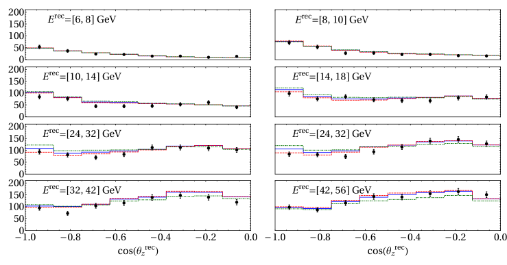
Figure 4: Event distributions obtained for DeepCore in our numerical simulations as a function of the reconstructed values of the cosine of the zenith angle, for neutrinos in different reconstructed energy ranges. The lines have been obtained assuming a normal mass ordering, for the following values for the decoherence parameters: $\gamma_{21}=\gamma_{31}=2.3\cdot 10^{-23}$ GeV (solid blue line), $\gamma_{21}=\gamma_{31}=10^{-22}$ GeV (dot-dashed green line) and without decoherence (dashed red line). The observed data points Aartsen:2014yll are represented by the black dots, and the error bars indicate the statistical uncertainties for each bin.

In each bin, the number of events is computed as

$$N_{i}(E^{rec},\theta_{z}^{rec}) =\sum_{\pm,\alpha,\beta}\int dE\,d\cos\theta_{z}\,\phi^{\text{atm}}_{\alpha,\pm}(E,\theta_{z})\,P_{\alpha\beta}^{\pm}(E,\theta_{z})$$

$$A^{\text{eff}}_{i,\pm,\beta}(E,\theta_{z},E^{rec},\theta_{z}^{rec})$$

$$+N_{i,\mu}(E^{rec},\theta_{z}^{rec}).$$ (42)

Unlike for IceCube, at DeepCore muon tracks can be produced from $\nu_{\mu}\to\nu_{\mu}$ and $\nu_{e}\to\nu_{\mu}$ events. Moreover, the track-like event distributions at DeepCore will also receive partial contributions from cascades which are mis-identified as tracks: hence the sum over $\beta=e,\mu,\tau$ in eq. (42). Therefore, here $\phi^{\text{atm}}_{\alpha,\pm}$ stands for the atmospheric flux for neutrinos/antineutrinos of flavor $\alpha$ (where we have used the fluxes from ref. Honda:2015fha ), and $P_{\alpha\beta}^{\pm}$ refers to the neutrino/antineutrino oscillation probability in the channel $\nu_{\alpha}\to\nu_{\beta}$ for neutrinos (+) (or $\bar{\nu}_{\alpha}\to\bar{\nu}_{\beta}$, for antineutrinos (-)). The rejection efficiencies for the contamination are included in the detector response function $A^{\text{eff}}_{i,\pm,\beta}$, which now depends on the flavor $\beta$ of the interacting neutrino. Finally, an estimate of the atmospheric muons that overcome the selection criteria (taken from refs. Aartsen:2014yll ; IceCubeweb ) is also added for each bin in reconstructed variables, $N_{i,\mu}$.

Figure 4 shows the expected number of events for DeepCore obtained from our numerical simulations including decoherence, for $\gamma_{21}=\gamma_{31}=2.3\cdot 10^{-23}$ GeV (solid blue lines) and $\gamma_{21}=\gamma_{31}=10^{-22}$ GeV (dot-dashed green lines), as a function of $\cos\theta_{z}^{rec}$, for events in different reconstructed energy ranges. For simplicity, we have considered the $n=0$ case (that is, $\gamma_{ij}$ independent of the neutrino energy). The expected result without decoherence is also shown for comparison (dashed red lines), while the observed data Aartsen:2014yll are shown by the black dots.

In this work a Gaussian maximum likelihood is used to analyze the DeepCore data, performing a simultaneous fit on the following parameters: $\Delta m^{2}_{32},\,\theta_{23}$ and $\gamma_{ij}$. The rest of the oscillation parameters have been kept fixed to their current best-fit values from refs. nufit ; Esteban:2016qun . The systematics used in the fit are those associated with the flux, the detector response and the atmospheric muons given in ref. Aartsen:2014yll and are summarized in tab. 2. For each systematic uncertainty a pull term is added to the $\chi^{2}$ following the values listed in the table, except in the cases indicated as “Free” (when the corresponding nuisance parameter is allowed to float freely in the fit). We have checked that our analysis reproduces the confidence regions in the $\Delta m_{32}^{2}-\theta_{23}$ plane obtained by the DeepCore collaboration in ref. Aartsen:2014yll to a very good level of accuracy.

Table 2: Systematic errors used in our analysis of DeepCore data, taken from refs. Aartsen:2014yll ; YanezGarza:2014jia .

Source of uncertainty	Value
Flux - normalization	Free
Flux - energy dependence as $(E/E_{0})^{\eta}$	$\Delta\eta=0.05$
Flux - $(\nu_{e}+\bar{\nu}_{e})/(\nu_{\mu}+\bar{\nu}_{\mu})$ ratio	20%
Background - normalization	Free
DOM efficiency	10%
Optical properties of the ice	1%

Finally, it should be noted that our fit does not include the latest atmospheric data recently published by the DeepCore collaboration Aartsen:2017nmd . The new analysis uses a different data set (from April 2012 to May 2015) and a new implementation of systematic errors, which lead to smaller confidence regions in the $\Delta m^{2}_{32}-\theta_{23}$ plane. However, the detector response parameters and systematic errors used in the latest release have not been published yet. In view of the better results obtained for the standard three-family oscillation scenario, a similar improvement is to be expected if the analysis performed in this work were to be repeated using the latest DeepCore data.

5 Results

Following the procedure described in sec. 4 we have obtained the $\chi^{2}$ for every point in the parameter space. Marginalizing over the relevant mixing and mass parameters, namely, $\Delta m^{2}_{32}$ and $\theta_{23}$, the sensitivity of the data to $\gamma_{ij}$ parameters is determined by evaluating the $\sqrt{\Delta\chi^{2}}$, with $\Delta\chi^{2}\equiv\chi^{2}-\chi^{2}_{\text{min}}$, where $\chi^{2}_{\text{min}}$ is the value at the global minimum.

In this section we will only show the results obtained for NO, since we have checked that extremely similar results are obtained for IO after applying the mapping given in eq. (40). Nevertheless, in sec. 6 we will also provide the 95% confidence level (CL) bounds obtained in our numerical analysis for the IO case. The bounds obtained are in very good agreement with the mapping given in eq. (40).

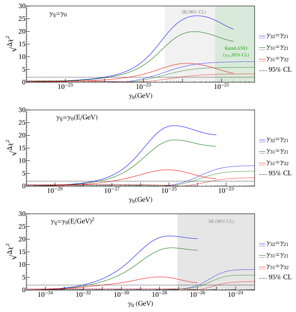
Figure 5: Values of the $\sqrt{\Delta\chi^{2}}$ as a function of the decoherence parameter for the Atmospheric limit (red), Solar limit I (green) and Solar limit II (blue) defined in sec. 3. The results obtained from our analysis of IceCube (DeepCore) data are denoted by the solid (dashed) lines. The three panels have been obtained for NO, assuming a different dependence on the neutrino energy: $n=0$ (top panel), $n=1$ (middle panel) and $n=2$ (bottom panel). The shaded regions are disfavored by previous analysis of SK Lisi:2000zt and KamLAND Gomes:2016ixi data, see text for details. The horizontal black line indicates the value of the $\sqrt{\Delta\chi^{2}}$ corresponding to 95% CL for 1 degree of freedom.

Figure 5 shows the obtained $\sqrt{\Delta\chi^{2}}$ as a function of $\gamma_{0}$ for the three limiting cases defined in sec. 3: (A) atmospheric limit, $\gamma_{0}=\gamma_{32}^{0}=\gamma_{31}^{0}$ (red curve); (B) solar limit I, $\gamma_{0}=\gamma_{21}^{0}=\gamma_{31}^{0}$ (green curve); and (C) solar limit II, $\gamma_{0}=\gamma_{21}^{0}=\gamma_{32}^{0}$ (blue curve). In all cases, the solid (dashed) lines correspond to the results obtained from our analysis of the IceCube (DeepCore) data, and each panel shows the results obtained assuming a different energy dependence for the decoherence parameters, see eq. (14): $n=0$ (top panel), $n=1$ (middle panel) and $n=2$ (bottom panel). The shaded regions are disfavored by previous analysis of SK Lisi:2000zt (90% CL) and KamLAND Gomes:2016ixi data (95% CL). As explained in sec. 3, the KamLAND constraints derived in Gomes:2016ixi apply to $\gamma_{12}^{0}$ (solar limits) while it is not clear to which $\gamma_{ij}$ the bounds from SK obtained in Lisi:2000zt would apply, since this depends on the true neutrino mass ordering (which is yet unknown).

Note that the size of the atmosphere has been neglected in our calculations (see A for details). This is a good approximation for small values of the decoherence parameters, but it starts to fail if the decoherence effects are large enough to affect neutrinos with $\cos\theta_{z}>0$. Therefore, in the case of IceCube we have shown our results only in the region where this approximation holds. In the case of DeepCore, due to the smaller energies considered, our approximation has no impact on the results even for large values of the decoherence parameters. Therefore, the approximation has only an impact on the IceCube results in a region of the decoherence parameter space which is already ruled out either by DeepCore or other experiments.

Figure 5 shows that for both DeepCore and IceCube the best sensitivity is achieved for the solar limits (B) and (C) while the weakest limit is obtained in the atmospheric limit (A). In particular, the strongest bound is obtained for (C). This is in agreement with the behaviour of the oscillation probability in presence of strong matter effects, discussed in sec. 3. On one hand, as shown in sec. 3, for NO the decoherence effects are mainly driven by $\gamma_{21}$ in the neutrino channel and $\gamma_{32}$ in the antineutrino channel. On the other hand, the number of antineutrino events is going to be suppressed with respect to the neutrino case, due to the smaller cross section and flux. Hence, the best sensitivity is expected for case (C), where $\gamma_{0}=\gamma_{21}^{0}=\gamma_{32}^{0}$, since both neutrinos and antineutrinos are sensitive to decoherence effects. Conversely, in case (B), where $\gamma_{0}=\gamma_{21}^{0}=\gamma_{31}^{0}$, only neutrinos are sensitive to decoherence effects, and therefore some sensitivity is lost with respect to the results for case (C). Finally, in case (A), with $\gamma_{0}=\gamma_{32}^{0}=\gamma_{31}^{0}$, the bounds come mainly from the impact of decoherence on the antineutrino event rates and, since these are much smaller than in the neutrino case, the obtained bounds are much weaker when compared to the results obtained in case (B).

Figure 5 shows a flat asymptotic feature of the DeepCore’s $\sqrt{\Delta\chi^{2}}$ for large values of $\gamma_{0}$, where the sensitivity becomes independent of $\gamma_{0}$. Conversely, for IceCube there is a decrease in sensitivity for values of $\gamma$ above a certain range: for example, for $n=0$ the best sensitivity is achieved for $\gamma_{0}\sim\mathcal{O}(10^{-22})$ GeV while it decreases for higher values. This behaviour can be understood as follows. For the neutrino energies observed at IceCube (above 100 GeV) the oscillation phases do not develop and the probabilities do not depend on the energy ($\cos\tilde{\Delta}_{ij}\approx 1$ in eq. (2.1)). Therefore, at IceCube the sensitivity to the decoherence effects comes from the observation of a non-standard behaviour of the number of events with the zenith angle alone. Naively, eq. (15) gives the values of $L$ and $\gamma$ that yield a large effect. Considering $n=0$, for example, where there is a one-to-one relation between the two, we get that for $\gamma_{0}\sim 10^{-22}$ GeV the effect will be maximal for distances of the order $L\sim\mathcal{O}(10^{3})$ km. This is the typical distance traveled by atmospheric neutrinos crossing the Earth and therefore the sensitivity of IceCube is maximized in this range. Conversely, for larger (smaller) values of $\gamma_{0}$, only neutrinos coming from the most horizontal (vertical) directions are affected, leading to a reduced impact on the $\chi^{2}$.

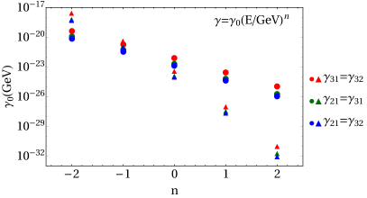
Figure 6: 95% CL bounds on the decoherence parameters $\gamma_{0}$, for NO, as a (discrete) function of the power-law index $n$ for the Atmospheric limit (red), Solar limit I (green) and Solar limit II (blue). The solid circles (triangles) correspond to the DeepCore (IceCube) analysis.

From the comparison between the different panels in fig. 5 we can see that the limits change considerably with the value of $n$, which parametrizes the energy dependence of the decoherence parameters (see eq. (14)). In particular, we observe in fig. 5 that the sensitivity improves with $n$ and that, as it is increased, the results for IceCube improve much faster (compared to DeepCore) due to the much higher neutrino energies considered in this case. The behaviour of the sensitivities with the value of $n$ is better appreciated in fig. 6, where we show the bounds obtained at 95% CL (for 1 degree of freedom) as a (discrete) function of the power-law index $n$, for $n=-2,-1,0,1$ and 2. The DeepCore bounds are represented by solid circles while the IceCube constraints are given by the solid triangles. The results seem to follow the linear relation

$$\ln(\gamma_{0}/\text{GeV})={\rm constant}-n\ln(E_{0}/\text{GeV}),$$ (43)

where $E_{0}\simeq$ 2.5 TeV (30 GeV) for IceCube (DeepCore). This can be understood as follows. Decoherence effects enter the oscillation probabilities only through the factor $\gamma L=\gamma_{0}(E/\text{GeV})^{n}L$, for any value of $n$. Naively, we expect that the sensitivity limit is obtained for $\gamma L\sim\mathcal{O}(1)$ (although the precise value will eventually depend on the neutrino mass ordering, on the particular $\gamma_{ij}$ which drives the sensitivity, and on the data set considered). Taking the logarithm of $\gamma_{0}(E/\text{GeV})^{n}L$ = constant, we reproduce eq. (43). At first approximation, the value of $E_{0}$ in eq. (43) can be estimated as the average energy of the IceCube and DeepCore event distributions, $\langle E\rangle$, as

$$\langle E\rangle\equiv\frac{\displaystyle\int\frac{dN}{dE}EdE}{\displaystyle\int\frac{dN}{dE}dE}\ ,$$ (44)

where $dN/dE$ is the event number distribution. This leads to $\langle E\rangle\simeq 4$ TeV ($40$ GeV) for IceCube (DeepCore), which are in the right ballpark although somewhat different from the values of $E_{0}$ giving the best fit to the data shown in fig. 6. Nevertheless, we find these to be in reasonable agreement, given our naive estimation of $E_{0}$ as the mean energy for each experiment.

6 Summary and Conclusions

Normal Ordering aaaaaaaa		$n=-2$	$n=-1$	$n=0$	$n=1$	$n=2$
	IceCube (this work)
	Atmospheric ($\gamma_{31}=\gamma_{32}$)	$2.8\cdot 10^{-18}$	$4.2\cdot 10^{-21}$	$\mathbf{4.0\cdot 10^{-24}}$	$\mathbf{1.0\cdot 10^{-27}}$	$\mathbf{1.0\cdot 10^{-31}}$
	Solar I ($\gamma_{31}=\gamma_{21}$)	$6.8\cdot 10^{-19}$	$1.2\cdot 10^{-21}$	$\mathbf{1.3\cdot 10^{-24}}$	$\mathbf{3.5\cdot 10^{-28}}$	$\mathbf{1.9\cdot 10^{-32}}$
	Solar II ($\gamma_{32}=\gamma_{21}$)	$5.2\cdot 10^{-19}$	$9.2\cdot 10^{-22}$	$9.7\cdot 10^{-25}$	$2.4\cdot 10^{-28}$	$9.0\cdot 10^{-33}$
	DeepCore (this work)
	Atmospheric ($\gamma_{31}=\gamma_{32}$)	$\mathbf{4.3\cdot 10^{-20}}$	$2.0\cdot 10^{-21}$	$8.2\cdot 10^{-23}$	$3.0\cdot 10^{-24}$	$1.1\cdot 10^{-25}$
	Solar I ($\gamma_{31}=\gamma_{21}$)	$\mathbf{1.2\cdot 10^{-20}}$	$5.4\cdot 10^{-22}$	$2.1\cdot 10^{-23}$	$6.6\cdot 10^{-25}$	$2.0\cdot 10^{-26}$
	Solar II ($\gamma_{32}=\gamma_{21}$)	$7.5\cdot 10^{-21}$	$3.5\cdot 10^{-22}$	$1.4\cdot 10^{-23}$	$4.2\cdot 10^{-25}$	$1.1\cdot 10^{-26}$
Inverted Ordering aaaaa	IceCube (this work)
	Atmospheric ($\gamma_{31}=\gamma_{32}$)	$6.8\cdot 10^{-19}$	$1.2\cdot 10^{-21}$	$\mathbf{1.3\cdot 10^{-24}}$	$\mathbf{3.5\cdot 10^{-28}}$	$\mathbf{1.9\cdot 10^{-32}}$
	Solar I ($\gamma_{31}=\gamma_{21}$)	$5.2\cdot 10^{-19}$	$9.2\cdot 10^{-22}$	$9.8\cdot 10^{-25}$	$2.4\cdot 10^{-28}$	$9.0\cdot 10^{-33}$
	Solar II ($\gamma_{32}=\gamma_{21}$)	$2.8\cdot 10^{-18}$	$4.2\cdot 10^{-21}$	$\mathbf{4.1\cdot 10^{-24}}$	$\mathbf{1.0\cdot 10^{-27}}$	$\mathbf{1.0\cdot 10^{-31}}$
	DeepCore (this work)
	Atmospheric ($\gamma_{31}=\gamma_{32}$)	$\mathbf{1.4\cdot 10^{-20}}$	$5.8\cdot 10^{-22}$	$2.2\cdot 10^{-23}$	$7.5\cdot 10^{-25}$	$2.3\cdot 10^{-26}$
	Solar I ($\gamma_{31}=\gamma_{21}$)	$8.3\cdot 10^{-21}$	$3.6\cdot 10^{-22}$	$1.4\cdot 10^{-23}$	$4.7\cdot 10^{-25}$	$1.3\cdot 10^{-26}$
	Solar II ($\gamma_{32}=\gamma_{21}$)	$\mathbf{5.0\cdot 10^{-20}}$	$2.3\cdot 10^{-21}$	$9.4\cdot 10^{-23}$	$3.3\cdot 10^{-24}$	$1.2\cdot 10^{-25}$
	Previous Bounds
	SK (two families) Lisi:2000zt		$2.4\cdot 10^{-21}$	$4.2\cdot 10^{-23}$		$1.1\cdot 10^{-27}$
	MINOS ($\gamma_{31},\gamma_{32}$) deOliveira:2013dia		$\mathbf{2.5\cdot 10^{-22}}$	$1.1\cdot 10^{-22}$	$2\cdot 10^{-24}$
	KamLAND ($\gamma_{21}$) Gomes:2016ixi		$\mathbf{3.7\cdot 10^{-24}}$	$6.8\cdot 10^{-22}$	$1.5\cdot 10^{-19}$

Table 3: DeepCore/IceCube bounds on $\gamma_{ij}^{0}$ in GeV ($\gamma_{ij}=\gamma_{ij}^{0}(E/\text{GeV})^{n}$), at the $95\%$ CL (1 degree of freedom), for both normal and inverted ordering as indicated. Previous constraints are also provided for comparison, and the dominant limit in each case is highlighted in bold face (notice that we considered the most conservative bound from the two solar limits).

In this work, we have derived strong limits on non-standard neutrino decoherence parameters in both the solar and atmospheric sectors from the analysis of IceCube and DeepCore atmospheric neutrino data. Our analysis includes matter effects in a consistent manner within a three-family oscillation framework, unlike most past literature on this topic. In sec. 2 we have developed a general formalism, dividing the matter profile into layers of constant density, which permits to study decoherence effects in neutrino oscillations affected by matter effects in a non-adiabatic regime. Our analysis shows that the matter effects are extremely relevant for atmospheric neutrino oscillations and their importance in order to correctly interpret the two-family limits obtained previously in the literature, as outlined in sec. 3.

We have found that the sensitivity to decoherence effects depends strongly on the neutrino mass ordering and on whether the sensitivity is dominated by the neutrino or antineutrino event rates. For neutrinos, the decoherence effects at high energies are mainly driven by $\gamma_{21}$ ($\gamma_{31}$) for normal (inverted) ordering, while in the antineutrino case they are essentially controlled by $\gamma_{32}$ ($\gamma_{21}$) for normal (inverted) ordering. This means that, considering a three-family framework including matter effects is essential when decoherence effects in atmospheric neutrino oscillations are studied. Our results are summarized in tab. 3, together with the most relevant bounds present in the literature. Table 3 provides the 95% CL bounds extracted from our analysis of DeepCore and IceCube atmospheric neutrino data, for both normal and inverted ordering, and for the three limiting cases considered in this work: (A) atmospheric limit ($\gamma_{21}=0$), (B) solar limit I ($\gamma_{32}=0$) and (C) solar limit II ($\gamma_{31}=0$). In B we show that the bounds derived in these limits correspond to the most conservative results that can be extracted in the general case.

In this work, we considered a general dependence of the decoherence parameters with the energy, as $\gamma_{ij}=\gamma_{ij}^{0}\left(E/\text{GeV}\right)^{n}$ with $n=\pm 2,0,\pm 2$. Our results improve over previous bounds for most of the cases studied, with the exception of the $n=-1$ case. For $n=-1$, KamLAND gives the dominant bound on $\gamma_{21}$ while MINOS gives the strongest constraints on $\gamma_{31}$ and $\gamma_{32}$ (indeed, both KamLAND and MINOS are also expected to give the strongest bound for $n=-2$, although to the best of our knowledge no analysis has been performed for this case yet). We have found that DeepCore considerably improves the present bounds in the solar sector ($\gamma_{21}$) for $n=0,1,2$ and gives a constraint in the atmospheric sector comparable to the SK limit, although a factor $2$ weaker, in the $n=0$ case. Our results show that, for $n=0$ (which is the case most commonly considered in the literature), IceCube improves the bound on $\gamma_{31}$ and $\gamma_{32}$ in (more than) one order of magnitude with respect to the SK constraint, obtained in a simplified two-family approximation, and by more than one order (almost two orders) of magnitude for NO (IO) with respect to the KamLAND constraint on $\gamma_{21}$. In particular, we find that the reference value for $\gamma_{23}$ considered in ref. Coelho:2017zes to explain the small tension previously reported between NOvA and SK data is indeed already excluded by IceCube data. Regarding the cases with $n=1,2$, we find that the sensitivity of IceCube is particularly strong. For instance, IceCube improves the bound from KamLAND on $\gamma_{21}$ by almost 9 (8) orders of magnitude for $n=1$ and NO (IO), while for $n=2$ the bound on $\gamma_{31}$ and $\gamma_{32}$ is improved in 4 (5) orders of magnitude with respect to the SK limit for NO (IO).

Appendix A Computation of oscillation probabilities in three layers

The simulation of atmospheric neutrino experiments is computationally demanding in the standard three-family scenario, and even more if decoherence effects are included in the analysis. Therefore, due to the cost of implementing a large number of layers for the PREM profile density, in this work we consider a simplified three-layer model for the Earth matter density profile assuming a core and Earth radii of 3321 km and 6371 km, respectively. The values of the matter densities of the inner layer (core) and the outer layer (mantle) are taken to be around $\rho=12$ g/cm³ and $4.6$ g/cm³, respectively. However, their values are slightly adjusted depending on the distance traveled by the neutrinos to match as close as possible the profile of the PREM model Dziewonski:1981xy . Note that, in our simulations, we have not considered the atmosphere as an additional layer. This is a good approximation for neutrinos going upwards in the detector ($\cos\theta_{z}<0$), but is not a valid approximation in the region $\cos\theta_{z}>0$. This has only an impact on the IceCube results for extremely large values of the decoherence parameters, which are already ruled out either by other experiments or by DeepCore.

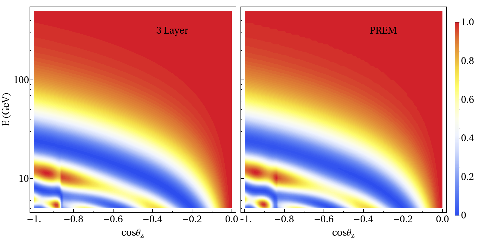
Figure 7: Oscillograms for $P_{\mu\mu}$ without decoherence, considering our three-layer approximation (left panel) and the PREM model (right panel) for the Earth matter density profile.

In fig. 7 we compare the results obtained for the oscillation probability for our modified three-layer approximation (left panel) against the exact numerical results using the full Preliminary Reference Earth Model (PREM) profile Dziewonski:1981xy (right panel), which divides the Earth into eleven layers where the matter density in each layer is given by a polynomial function of the distance traveled. In this figure, the results are shown for the standard three-family scenario with no decoherence, in order to illustrate the accuracy of our three-layer approximation. The results are shown as a neutrino oscillogram, which represents the oscillation probability in the $P_{\mu\mu}$ channel in terms of energy and the zenith angle $\theta_{z}$ of the incoming neutrino. In this figure, a normal mass ordering was assumed, together with the following input values for the oscillation parameters nufit ; Esteban:2016qun : $\Delta m^{2}_{21}=7.4\cdot 10^{-5}$ eV², $\Delta m^{2}_{31}=2.515\cdot 10^{-3}$ eV², $\theta_{12}=33.62^{\circ}$, $\theta_{13}=8.54^{\circ}$, $\sin^{2}\theta_{23}=0.51$, and $\delta=234^{\circ}$.

As can be seen from the comparison between the two panels, some small differences take place but only in a restricted range of values of energy and zenith angle. Therefore, we conclude that the agreement between the probabilities obtained using the exact PREM model (right) and our approximate three-layer model (left) is sufficiently good for the purposes of this work. We have also checked that, using our simplified three-layer model applied to the standard case without decoherence, we are able to reproduce up to a very good approximation the DeepCore oscillation fit for the atmospheric parameters $\theta_{23}$ and $\Delta m^{2}_{32}$ Aartsen:2014yll .

Appendix B Five-dimensional analysis

The $\gamma_{ij}$ are not completely independent parameters, see eq. (8). In order to simplify the analysis, in this work we have focused on three different representative cases: (A) Atmospheric limit, $\gamma_{21}=0$ ($\gamma_{32}=\gamma_{31}$); (B) Solar limit I, $\gamma_{32}=0$ ($\gamma_{21}=\gamma_{31}$); and (C) Solar limit II, $\gamma_{31}=0$ ($\gamma_{21}=\gamma_{32}$). Considering these one-$\gamma_{ij}$-dominated cases is expected to be a very good approximation in view of eqs. (33)-(36). Nevertheless, in this appendix we will show that the results obtained in these simplified scenarios also apply to the more general case in which the three $\gamma_{ij}$ are different from zero.

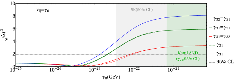
Figure 8: $\sqrt{\Delta\chi^{2}}$ obtained from the five-dimensional DeepCore analysis as a function of $\gamma_{21}$ (dashed green curve) and $\gamma_{31}$ (dashed red curve), marginalizing over the rest of the free parameters, for $n=0$ and NO. The $\sqrt{\Delta\chi^{2}}$ for the Atmospheric (solid red curve), Solar I (solid green curve) and Solar II (solid blue curve) limits is also shown.

Let us assume that just one $D_{m}$ matrix contributes to the decoherence term of the evolution equations given by eq. (2). In such a case, one of the $\gamma_{ij}$ parameters is a function of the other two $\gamma_{ij}$. Without loss of generality, if we choose $\gamma_{21}$ and $\gamma_{31}$ as our free parameters, $\gamma_{32}$ is then given by

$$\gamma_{32}=\left(\sqrt{\gamma_{21}}\pm\sqrt{\gamma_{31}}\right)^{2}.$$ (45)

In order to understand how general are the results presented in sec. 5, we have performed a five-dimensional analysis varying $\gamma_{21},\,\gamma_{31},\,\theta_{23}$ and $\Delta m^{2}_{32}$ in the fit, and imposing the constraint given by the equation above. In fig. 8 we show the $\sqrt{\Delta\chi^{2}}$ obtained from the five-dimensional DeepCore analysis as a function of $\gamma_{21}$ (dashed green curve) and $\gamma_{31}$ (dashed red curve), marginalizing over the rest of the free parameters, for the $n=0$ case (the same conclusions apply to the other cases studied in this work). For the sake of comparison, the $\sqrt{\Delta\chi^{2}}$ associated to the atmospheric (solid red curve), solar I (solid green curve) and solar II (solid blue curve) limits is also included in the same figure. NO was assumed but the results can be easily extrapolated to the IO case using the mapping given in eq. (40).

Figure 8 shows that the five-dimensional $\sqrt{\Delta\chi^{2}}$ distribution projected into $\gamma_{31}$ coincides with the Atmospheric limit one, while when it is projected into $\gamma_{21}$ resembles the most conservative of the two solar limits. This is due to the marginalization over the parameters which are not shown. For instance, in the case of $\gamma_{21}$ the marginalization selects, between the two solar limits, the most conservative result. We conclude therefore that our analysis distinguishing the three limits (A), (B) and (C), provides the most conservative bounds that can be applied to the general case in which the three $\gamma_{ij}$ are different from zero.

References

- (1) Daya Bay collaboration, F. P. An et al., New Measurement of Antineutrino Oscillation with the Full Detector Configuration at Daya Bay, Phys. Rev. Lett. 115 (2015) 111802, [1505.03456].
- (2) A. Izmaylov, “T2K Neutrino Experiment. Recent Results and Plans. Talk given at the Flavour Physics Conference, Quy Nhon, Vietnam, August 13–19, 2017.” http://v17flavour.in2p3.fr/ThursdayAfternoon/Izmaylov.pdf.
- (3) Alexander Radovic, “Results from NOvA, Fermilab Joint Experimental-Theoretical Physics Seminar, January 12, 2018.” http://theory.fnal.gov/events/event/results-from-nova/.
- (4) “NuFIT 3.2 (2018).” Results available at: http://www.nu-fit.org.
- (5) I. Esteban, M. C. Gonzalez-Garcia, M. Maltoni, I. Martinez-Soler and T. Schwetz, Updated fit to three neutrino mixing: exploring the accelerator-reactor complementarity, JHEP 01 (2017) 087, [1611.01514].
- (6) F. Benatti and R. Floreanini, Open system approach to neutrino oscillations, JHEP 02 (2000) 032, [hep-ph/0002221].
- (7) E. Lisi, A. Marrone and D. Montanino, Probing possible decoherence effects in atmospheric neutrino oscillations, Phys. Rev. Lett. 85 (2000) 1166–1169, [hep-ph/0002053].
- (8) A. M. Gago, E. M. Santos, W. J. C. Teves and R. Zukanovich Funchal, Quantum dissipative effects and neutrinos: Current constraints and future perspectives, Phys. Rev. D63 (2001) 073001, [hep-ph/0009222].
- (9) A. M. Gago, E. M. Santos, W. J. C. Teves and R. Zukanovich Funchal, A Study on quantum decoherence phenomena with three generations of neutrinos, hep-ph/0208166.
- (10) D. Morgan, E. Winstanley, J. Brunner and L. F. Thompson, Probing quantum decoherence in atmospheric neutrino oscillations with a neutrino telescope, Astropart. Phys. 25 (2006) 311–327, [astro-ph/0412618].
- (11) D. Hooper, D. Morgan and E. Winstanley, Probing quantum decoherence with high-energy neutrinos, Phys. Lett. B609 (2005) 206–211, [hep-ph/0410094].
- (12) G. L. Fogli, E. Lisi, A. Marrone, D. Montanino and A. Palazzo, Probing non-standard decoherence effects with solar and KamLAND neutrinos, Phys. Rev. D76 (2007) 033006, [0704.2568].
- (13) Y. Farzan, T. Schwetz and A. Y. Smirnov, Reconciling results of LSND, MiniBooNE and other experiments with soft decoherence, JHEP 07 (2008) 067, [0805.2098].
- (14) P. Bakhti, Y. Farzan and T. Schwetz, Revisiting the quantum decoherence scenario as an explanation for the LSND anomaly, JHEP 05 (2015) 007, [1503.05374].
- (15) G. Balieiro Gomes, M. M. Guzzo, P. C. de Holanda and R. L. N. Oliveira, Parameter Limits for Neutrino Oscillation with Decoherence in KamLAND, Phys. Rev. D95 (2017) 113005, [1603.04126].
- (16) R. L. N. Oliveira, Dissipative Effect in Long Baseline Neutrino Experiments, Eur. Phys. J. C76 (2016) 417, [1603.08065].
- (17) J. A. B. Coelho, W. A. Mann and S. S. Bashar, Nonmaximal mixing at NOvA from neutrino decoherence, Phys. Rev. Lett. 118 (2017) 221801, [1702.04738].
- (18) J. a. A. B. Coelho and W. A. Mann, Decoherence, matter effect, and neutrino hierarchy signature in long baseline experiments, Phys. Rev. D96 (2017) 093009, [1708.05495].
- (19) J. A. Carpio, E. Massoni and A. M. Gago, Revisiting quantum decoherence in the matter neutrino oscillation framework, Phys. Rev. D97 (2018) no.11, 115017, [1711.03680]
- (20) C. Giunti and C. W. Kim, Coherence of neutrino oscillations in the wave packet approach, Phys. Rev. D58 (1998) 017301, [hep-ph/9711363].
- (21) Daya Bay collaboration, F. P. An et al., Study of the wave packet treatment of neutrino oscillation at Daya Bay, Eur. Phys. J. C77 (2017) 606, [1608.01661].
- (22) S. W. Hawking, Breakdown of Predictability in Gravitational Collapse, Phys. Rev. D14 (1976) 2460–2473.
- (23) J. R. Ellis, J. S. Hagelin, D. V. Nanopoulos and M. Srednicki, Search for Violations of Quantum Mechanics, Nucl. Phys. B241 (1984) 381. [,580(1983)].
- (24) S. B. Giddings and A. Strominger, Loss of Incoherence and Determination of Coupling Constants in Quantum Gravity, Nucl. Phys. B307 (1988) 854–866.
- (25) Super-Kamiokande collaboration, Y. Fukuda et al., Evidence for oscillation of atmospheric neutrinos, Phys. Rev. Lett. 81 (1998) 1562–1567, [hep-ex/9807003].
- (26) Super-Kamiokande collaboration, Y. Fukuda et al., Measurement of a small atmospheric muon-neutrino / electron-neutrino ratio, Phys. Lett. B433 (1998) 9–18, [hep-ex/9803006].
- (27) Super-Kamiokande collaboration, Y. Fukuda et al., Study of the atmospheric neutrino flux in the multi-GeV energy range, Phys. Lett. B436 (1998) 33–41, [hep-ex/9805006].
- (28) Super-Kamiokande collaboration, Y. Fukuda et al., Measurement of the flux and zenith angle distribution of upward through going muons by Super-Kamiokande, Phys. Rev. Lett. 82 (1999) 2644–2648, [hep-ex/9812014].
- (29) KamLAND collaboration, K. Eguchi et al., First results from KamLAND: Evidence for reactor anti-neutrino disappearance, Phys. Rev. Lett. 90 (2003) 021802, [hep-ex/0212021].
- (30) KamLAND collaboration, S. Abe et al., Precision Measurement of Neutrino Oscillation Parameters with KamLAND, Phys. Rev. Lett. 100 (2008) 221803, [0801.4589].
- (31) M. M. Guzzo, P. C. de Holanda and R. L. N. Oliveira, Quantum Dissipation in a Neutrino System Propagating in Vacuum and in Matter, Nucl. Phys. B908 (2016) 408–422, [1408.0823].
- (32) R. L. N. de Oliveira, M. M. Guzzo and P. C. de Holanda, Quantum Dissipation and Violation in MINOS, Phys. Rev. D89 (2014) 053002, [1401.0033].
- (33) MINOS collaboration, P. Adamson et al., First direct observation of muon antineutrino disappearance, Phys. Rev. Lett. 107 (2011) 021801, [1104.0344].
- (34) MINOS collaboration, P. Adamson et al., Measurement of the Neutrino Mass Splitting and Flavor Mixing by MINOS, Phys. Rev. Lett. 106 (2011) 181801, [1103.0340].
- (35) MINOS collaboration, P. Adamson et al., An improved measurement of muon antineutrino disappearance in MINOS, Phys. Rev. Lett. 108 (2012) 191801, [1202.2772].
- (36) G. Lindblad, On the Generators of Quantum Dynamical Semigroups, Commun. Math. Phys. 48 (1976) 119.
- (37) T. Banks, L. Susskind and M. E. Peskin, Difficulties for the Evolution of Pure States Into Mixed States, Nucl. Phys. B244 (1984) 125–134.
- (38) M. C. Gonzalez-Garcia and M. Maltoni, Status of Oscillation plus Decay of Atmospheric and Long-Baseline Neutrinos, Phys. Lett. B663 (2008) 405–409, [0802.3699].
- (39) P. B. Denton, H. Minakata and S. J. Parke, Compact Perturbative Expressions For Neutrino Oscillations in Matter, JHEP 06 (2016) 051, [1604.08167].
- (40) P. B. Denton, H. Minakata and S. J. Parke, ”Compact Perturbative Expressions for Neutrino Oscillations in Matter: II”, JHEP 1806 (2018) 109, [1801.06514].
- (41) J. T. Pantaleone, Constraints on three neutrino mixing from atmospheric and reactor data, Phys. Rev. D49 (1994) R2152–R2155, [hep-ph/9310363].
- (42) E. K. Akhmedov, M. Maltoni and A. Yu. Smirnov, 1-3 leptonic mixing and the neutrino oscillograms of the Earth, JHEP 05 (2007) 077, [hep-ph/0612285].
- (43) IceCube collaboration, M. G. Aartsen et al., The IceCube Neutrino Observatory: Instrumentation and Online Systems, JINST 12 (2017) P03012, [1612.05093].
- (44) IceCube collaboration, M. G. Aartsen et al., Determining neutrino oscillation parameters from atmospheric muon neutrino disappearance with three years of IceCube DeepCore data, Phys. Rev. D91 (2015) 072004, [1410.7227].
- (45) IceCube collaboration, M. G. Aartsen et al., Searches for Sterile Neutrinos with the IceCube Detector, Phys. Rev. Lett. 117 (2016) 071801, [1605.01990].
- (46) B. J. P. Jones, Sterile neutrinos in cold climates. PhD thesis, Massachusetts Institute of Technology, 2015. available from http://hdl.handle.net/1721.1/101327.
- (47) C. A. Argüelles, New Physics with Atmospheric Neutrinos. PhD thesis, University of Wisconsin, Madison, 2015. PhD Thesis, available at https://docushare.icecube.wisc.edu/dsweb/Get/Document-75669/tesis.pdf.
- (48) J. P. Yanez Garza, Measurement of neutrino oscillations in atmospheric neutrinos with the IceCube DeepCore detector. PhD thesis, Humboldt U., Berlin, 2014. PhD thesis, available at: http://edoc.hu-berlin.de/dissertationen/yanez-garza-juan-pablo-2014-06-02/PDF/yanez-garza.pdf.
- (49) IceCube collaboration, M. G. Aartsen et al., Search for Astrophysical Tau Neutrinos in Three Years of IceCube Data, Phys. Rev. D93 (2016) 022001, [1509.06212].
- (50) “IceCube collaboration webpage.” https://icecube.wisc.edu/science/data.
- (51) C. Weaver, Evidence for Astrophysical Muon Neutrinos from the Northern Sky. PhD thesis, University of Wisconsin, Madison, 2015. PhD thesis, available at https://docushare.icecube.wisc.edu/dsweb/Get/Document-73829/weaver_thesis_2015.pdf.
- (52) M. Honda, M. Sajjad Athar, T. Kajita, K. Kasahara and S. Midorikawa, Atmospheric neutrino flux calculation using the NRLMSISE-00 atmospheric model, Phys. Rev. D92 (2015) 023004, [1502.03916].
- (53) IceCube collaboration, M. G. Aartsen et al., Measurement of Atmospheric Neutrino Oscillations at 6–56 GeV with IceCube DeepCore, Phys. Rev. Lett. 120 (2018) 071801, [1707.07081].
- (54) A. M. Dziewonski and D. L. Anderson, Preliminary reference earth model, Phys. Earth Planet. Interiors 25 (1981) 297–356.