Spitzer Opens New Path to Break Classic Degeneracy for Jupiter-Mass Microlensing Planet OGLE-2017-BLG-1140Lb

Abstract

We analyze the combined Spitzer and ground-based data for OGLE-2017-BLG-1140 and show that the event was generated by a Jupiter-class $(m_{p}\simeq 1.6\,M_{\rm jup})$ planet orbiting a mid-late M dwarf $(M\simeq 0.2\,M_{\odot})$ that lies $D_{LS}\simeq 1.0\,{\rm kpc}$ in the foreground of the microlensed, Galactic-bar, source star. The planet-host projected separation is $a_{\perp}\simeq 1.0\,{\rm AU}$, i.e., well-beyond the snow line. By measuring the source proper motion ${\mbox{\boldmath$\mu$}}_{s}$ from ongoing, long-term OGLE imaging, and combining this with the lens-source relative proper motion ${\mbox{\boldmath$\mu$}}_{\rm rel}$ derived from the microlensing solution, we show that the lens proper motion ${\mbox{\boldmath$\mu$}}_{l}={\mbox{\boldmath$\mu$}}_{\rm rel}+{\mbox{\boldmath$\mu$}}_{s}$ is consistent with the lens lying in the Galactic disk, although a bulge lens is not ruled out. We show that while the Spitzer and ground-based data are comparably well fitted by planetary (i.e., binary-lens, 2L1S) models and by binary-source (1L2S) models, the combination of Spitzer and ground-based data decisively favor the planetary model. This is a new channel to resolve the 2L1S/1L2S degeneracy, which can be difficult to break in some cases.

1 Introduction

The degeneracy between binary-lens/single-source (2L1S) and single-lens/binary-source (1L2S) microlensing events, first noted by Gaudi (1998), has continually grown in importance and complexity over the first 15 years of microlensing planet detections, particularly as these have reached toward lower planet-host mass-ratio planets. As originally formulated by Gaudi (1998), a 1L2S event can mimic a 2L1S event if the second source is much fainter than the first and if the lens happens to pass much closer to it. In this case, the second source gives rise to a smooth, short-lived, low-amplitude bump, as it very briefly becomes highly magnified. Any putative planetary signal that is consistent with such a smooth short-lived bump must therefore be vetted against the 1L2S explanation. This already became an issue for the third microlensing planet, OGLE-2005-BLG-390Lb (Beaulieu et al., 2006), for which the smooth bump was actually generated by a “Cannae” type “Hollywood” event (Hwang et al., 2018), in which a very large source completely envelops the planetary caustic. For the actual case of OGLE-2005-BLG-390Lb, the 1L2S solution was ruled out ($\Delta\chi^{2}>50$). However, in the course of their systematic study of all archival low-mass-ratio $(q<10^{-4})$ microlensing planets, Udalski et al. (2018) showed that had the mass ratio been smaller, $\log(q^{\prime}/q)<-0.2$, then the 2L1S and 1L2S models could not have been reliably distinguished.

Over the years, it has become clear that a variety of other microlensing-planet geometries can induce smooth bumps that can potentially be confused with 1L2S geometries. Bond et al. (2017) and Shvartzvald et al. (2017) analyzed a smooth bump in OGLE-2016-BLG-1195 and both showed that it was due to the source passing over a smooth “ridge” in the magnification pattern between the central and planetary caustic (“wide planet” solution) or over a smooth ridge extending from the central caustic (“close planet” solution). Again, however, Udalski et al. (2018) showed that the 2L1S and 1L2S solutions could not have been distinguished if the planet mass ratio had been lower by $\log(q^{\prime}/q)<-0.3$.

Both of these forms of the degeneracy are likely to become more important in the future. Zhu et al. (2014) showed that in the era of pure-survey microlensing planet detections, half of all “detectable” planets (based on $\chi^{2}$ criterion) are likely to be non-caustic crossing events (i.e., broadly similar to OGLE-2016-BLG-1195), which will generically induce smooth bumps, as opposed to the sudden jumps that usually characterize caustic crossings, which are present in a substantial majority of published planetary microlensing events. Moreover, it is not necessary to fully envelop the caustic to produce a smooth bump in a caustic-crossing event: Hwang et al. (2018) showed that “von Schlieffen” type Hollywood events, in which the source only partially envelops the caustic, can produce very similar light curves to “Cannae” events.

Furthermore, new forms of this degeneracy are being discovered. Jung et al. (2017) showed that a 1L2S event with a source-flux ratio $q_{f}\simeq 2$ could be broadly mimicked by a planetary microlensing geometry. In this case, the 2L1S geometry was ruled out by $\Delta\chi^{2}>500$, so strictly speaking the solutions were not “degenerate”. Nevertheless, the fact that much more complex binary-lens structures than “short-lived bumps” can be mimicked by binary-source geometries should serve as a broad caution when analyzing events.

Finally, Hwang et al. (2017) found yet another path to this degeneracy in their analysis of OGLE-2015-BLG-1459. The first point to note about this event is that it had a three-fold degeneracy 3L1S versus 2L2S versus 1L3S. In the triple lens model, the third body was a “moon” that was detected in only one magnified point (albeit, a 0.4 mag deviation detected with very high confidence). Such single-point (or even few-point) deviations due to a planet can easily be confused with a “smooth bump”, even if the underlying light curve would reveal a pronounced caustic structure, just because of poor sampling.

The first line of defense against the 2L1S/1L2S degeneracy is simply $\Delta\chi^{2}$ between the two models. A few cases were mentioned above, but there are many others as well (e.g., Han et al. 2018). However, as discussed above, in the few published cases of low-$q$ events that were investigated by Udalski et al. (2018), the threshold for resolving this degeneracy did not lie far below the actual value of $q$.

A second line of defense is to measure the color difference of the (putative) two sources. Because light travels on geodesics, microlensing is intrinsically achromatic. The only exception would be if two stars (or two parts of a single star) were of different colors and were magnified by different amounts. The latter effect can occur if a single star is transited by a point lens or by a caustic from a binary lens. However, this is rather weak. Substantial chromaticity requires two sources of substantially different color and magnified by different amounts. The short-term “smooth bumps” that are the main source of ambiguity are well suited to this test. Recall that the 1L2S model generally requires that one of the sources is much fainter than the other and also much more highly magnified. Generally, fainter sources are redder (particularly if the brighter source is on the main sequence), so the light during the bump should be redder than on the rest of the light curve. For example, Hwang et al. (2017) confirmed the 1L3S interpretation using this effect for OGLE-2015-BLG-1459. However, if the primary source is a giant, then the secondary can have a similar color even if it is several orders of magnitude fainter. Moreover, as mentioned above, there are cases for which the source-flux ratio is actually close to unity (Jung et al., 2017). But the main impediment to this method is simply that alternate (usually $V$) band data are not typically taken at high-enough cadence to accurately measure the color of a short-lived smooth bump.

Here, we use Spitzer observations of the planetary microlensing event OGLE-2017-BLG-1140 to demonstrate the power of a new method to resolve the 2L1S/1L2S degeneracy that is based on space-based microlensing parallax.

2 Observations

OGLE-2017-BLG-1140 is at (RA,Dec) = (17:47:31.93,$-$24:31:21.6) corresponding to $(l,b)=(4.0,1.9)$. It was discovered and announced as a probable microlensing event by the OGLE Early Warning System (Udalski et al., 1994; Udalski, 2003) at UT 11:57 on 19 June 2017. The event lies in OGLE field BLG633 (Udalski et al., 2015b), for which OGLE observations were at a characteristic cadence of $\Gamma=1\,{\rm day^{-1}}$ using their 1.3m telescope at Las Campanas, Chile.

The Korea Microlensing Telescope Network (KMTNet, Kim et al. 2016) observed this field from its three 1.6m telescopes at CTIO (Chile, KMTC), SAAO (South Africa, KMTS) and SSO (Australia, KMTA), in its BLG19 field, implying that it was observed at a cadence of $\Gamma=1\,{\rm hr^{-1}}$ during the Spitzer season. The event was identified by KMTNet as SSO19M0601.004271.

The great majority of ground-based observations were carried out in the $I$ band with occasional $V$-band observations made solely to determine source colors. All reductions for the light curve analysis were conducted using variants of difference image analysis (DIA, Tomaney & Crotts 1996; Alard & Lupton 1998), specifically Woźniak (2000) and Albrow et al. (2009).

The event was also observed by Spitzer. As discussed in detail by Yee et al. (2015), Spitzer selections can be “objective”, “subjective”, or “secret”, which impacts how detected planets (and planet sensitivity) enter the Spitzer program to measure the Galactic distribution of planets (Gould et al., 2013, 2014, 2015a, 2015b, 2016). Events that meet certain pre-specified objective criteria must be observed, and consequently all planets detected during the event can enter the program sample. Events can be selected “subjectively” by the team for any reason and at any time. However, only planets (and simulated planets needed to calculate planet sensitivity) that do not generate significant signal in the data available at the time of the public announcement can enter the sample. The observational cadence and the conditions for stopping the observations must be specified at the time of the announcement. Events can also be chosen “secretly”, i.e., without announcement, and then later changed to “subjective” (if such a decision is subsequently made). In this case, the constraints on what is a “detectable” planet apply according to the date of the “subjective” announcement. Moreover, Spitzer observations taken before this date cannot be included in the determination of whether the microlens parallax is well-enough measured to enter the sample (Zhu et al., 2017).

OGLE-2017-BLG-1140 was chosen “secretly”, at UT 13:08 on 19 June, i.e., slightly more than one hour after it was announced by OGLE and about 8 minutes before the first Spitzer “upload” (i.e., when target coordinates are sent to Spitzer Operations). This selection was made by the upload subteam because the event appeared to be consistent with reaching relatively high magnification based on the data available at that time. The upload subteam does not generally have the authority to choose events subjectively, without giving the whole team an opportunity for a joint decision. The target entered the Spitzer Sun-angle window roughly 1.65 days after the first Spitzer observation, i.e., at UT 07:08 on 24 June. The event was announced “subjectively” at UT 16:23 on 25 June, i.e., about 33 hours later. Therefore, all Spitzer observations in this interval must be excluded from the determination of whether the Spitzer parallax is well measured, and of course if a planetary anomaly proves significantly detectable $(\Delta\chi^{2}=10)$ from data available prior to this announcement (HJD${}^{\prime}\equiv{\rm HJD}-2450000=7930.19$), then the planet must be excluded from the Galactic distribution sample.

In fact, these restrictions have almost no practical effect. There were only four Spitzer observations taken in this interval, and they do not contribute significantly to the parallax measurement. The last ground-based data point available at the time of the announcement was at ${\rm HJD}^{\prime}=7928.61$, at which point the light curve was perfectly consistent with a point lens. The event was first suspected to be anomalous on 5 July, but in retrospect this appears to be based on some points near peak that were impacted by close passage of the Moon. The anomaly was first recognized as due to a weak 2L1S perturbation or a 1L2S geometry on 13 July based on ground-based data. However, at that point, and also at a subsequent update when the event reached baseline, the 2L1S/1L2S degeneracy appeared insurmountable. The decision to pursue the analysis was made after inspecting the anomaly in the Spitzer data.

The Spitzer data were reduced using specially designed software (Calchi Novati et al., 2015b).

We follow the standard procedure (e.g. Yee et al. 2012) of rescaling error bars so that the $\chi^{2}/\mathrm{dof}$ for each data set is of order unity for the best model. For OGLE and KMTNet the rescaling factors are in the range 1.3-1.5, for Spitzer we evaluate a factor 2.6.

3 Light Curve Analysis

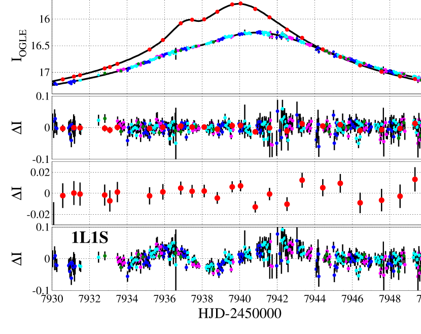
Figure 1: Light curve and binary-lens/single-source (2L1S) model and residuals of OGLE-2017-BLG-1140 (first four panels from the top). The overall difference between the Spitzer (which is transformed for display to the $I$-band magnitude system) and ground-based (OGLE, KMTA, KMTC, and KMTS) data yields the microlens parallax vector ${\mbox{\boldmath$\pi$}}_{\rm E}$. More subtle differences, such as the strength of the pre-peak “smooth bump” anomaly in both data sets, allow one to decisively rule out the competing class of single-lens/binary-source (1L2S) models. Note that the Spitzer residuals are shown again, separately, in the bottom panel because their error bars are substantially smaller than the range that must be displayed on the main residual panel. Bottom panel: residuals for 1L1S model for ground-based data only.

At glance, OGLE-2017-BLG-1140 deviates from the smooth, symmetric (single) point source-point-lens (1L1S) Paczyński (1986) shape. This is obvious from inspection of the Spitzer light curve, somewhat less so for ground-based data (see Figure 1). Still, for ground-based data only, a 1L1S model has a $\Delta\chi^{2}=915$ from the best planetary model discussed below, and the systematic deviations from the data are clearly visibile in the bottom panel of Figure 1. Based on the general appearance of its light curve, OGLE-2017-BLG-1140 could in principle be either 2L1S or 1L2S. However, because the correct model is actually 2L1S, we focus on that here and defer discussion of 1L2S models to Section 5.

We will eventually show that 2L1S solutions could be derived from either the ground-based or Spitzer data. However, we begin by reporting our actual path toward deriving the solution. As in the case of OGLE-2017-BLG-1130 (Wang et al., 2018), the binarity of the lens is much more apparent by eye in the Spitzer data, so we begin by conducting a grid search using these data only. The lens system is reasonably well described by six parameters $(t_{0},u_{0},t_{\rm E},s,q,\alpha)$. The first three (Paczyński, 1986) parameters are, respectively the time of closest approach to the center of mass, the impact parameter (normalized to $\theta_{\rm E}$) and the Einstein timescale, i.e., $t_{\rm E}=\theta_{\rm E}/\mu_{\rm rel}$, where ${\mbox{\boldmath$\mu$}}_{\rm rel}$ is the lens-source relative proper motion. The final three are the planet-host separation (in units of $\theta_{\rm E}$), the planet-host mass ratio, and the angle between the instantaneous planet-host axis and $\mu$. In fact, as we will show shortly, a seventh parameter can also be measured: $\rho\equiv\theta_{*}/\theta_{\rm E}$, where $\theta_{*}$ is the angular radius of the source. However, in order to quantify the robustness of this measurement and also to facilitate understanding of the information flow, we initially set $\rho=0$. In addition to these six geometric parameters, there are two flux parameters $(f_{s,j},f_{b,j})$ for each observatory, $j$. That is, we model the flux observed at each time $t_{i}$ by the $j$th observatory as $F_{j}(t_{i})=f_{s,j}A(t_{i};t_{0},u_{0},t_{\rm E},s,q,\alpha)+f_{b,j}$.

3.1 Six-Parameter Solutions ($\rho=0$)

The binary lens model is specified by the parameters of the caustic, $(s,q)$, and the angle of the trajectory, $\alpha$. In the caustic region, because of the divergences in the magnification map, the $\chi^{2}$ topology is however extremely complex and may present sharp variations along these parameters. Therefore, standard minimization procedures including Markov Chain Monte Carlo (MCMC) are not suitable tools to locate, starting from a generic position in the parameter space, the absolute minimum. This is not the case, on the other hand, for the single lens parameters for which the $\chi^{2}$ surface is smooth (in particular this holds for $\rho$ and explain why we run the grid with $\rho=0$). This is the reason why, lacking a plausible a priori intuition of the “right” binary lens model, we start the analysis with a blind-search grid in the binary lens parameter space. Once the $\chi^{2}$ minimum is identified within the grid search, we then run a final analysis with all the parameters left free to vary to fully characterize the solution. Specifically, we conduct a dense $40^{3}$ grid search on $[0\leq s<2]\times[-4\leq\log q<0]\times[0\leq\alpha<2\pi]$, and for each such triple we fit for the remaining three parameters. We model the light curves using the algorithm of Bozza (2010), which has a publicly available implementation. This grid search yields four minima at $(s,\log q)=(0.7,-1.8)$, $(0.8,-2.2)$, $(1.5,-2.2)$, and $(1.6,-1.4)$. We then seed these solutions into a MCMC (Dong et al., 2009) for which all parameters are allowed to vary. The two “close” ($s<1$) seeds both converge to the same solution, which is given in Table 1. The remaining two solutions, which are the corresponding “wide” $(s>1)$ variants of the close/wide $(s\leftrightarrow s^{-1})$ degeneracy (Griest & Safizadeh, 1998; Dominik, 1999), also converge. However, these prove not be viable, as we discuss further below.

To combine Spitzer and ground-based data, we must introduce two additional parameters, the two components of the vector microlens parallax (Gould, 1992b, 2000),

$${\mbox{\boldmath$\pi$}}_{\rm E}\equiv{\pi_{\rm rel}\over\theta_{\rm E}}\,{{\mbox{\boldmath$\mu$}}_{\rm rel}\over\mu_{\rm rel}}\,,$$ (1)

where $\pi_{\rm rel}\equiv{\rm AU}(D_{L}^{-1}-D_{S}^{-1})$ is the lens-source relative parallax. We evaluate ${\mbox{\boldmath$\pi$}}_{\rm E}$ in equatorial coordinates, i.e., ${\mbox{\boldmath$\pi$}}_{\rm E}=(\pi_{{\rm E},N},\pi_{{\rm E},E})$.

We make an initial estimate of ${\mbox{\boldmath$\pi$}}_{\rm E}$ by simultaneously fitting the ground and space data (with the anomaly excised) to a 1L1S model. We then seed the resulting ${\mbox{\boldmath$\pi$}}_{\rm E}$ as well as the Spitzer-based fit for the other six parameters $(t_{0},u_{0},t_{\rm E},s,q,\alpha)$ into a simultaneous fit to the ground-based and Spitzer data. The resulting solution is again shown in Table 1. This is the so-called “$(+,+)$” solution. See Section 3.2. In order to facilitate comparison with results in that section, we also show the corresponding “$(-,-)$” solution. Finally, we remove the Spitzer data and fit for six parameters only $(t_{0},u_{0},t_{\rm E},s,q,\alpha)$ using the ground-based data. This solution is also shown in Table 1.

Comparing the three solutions (Spitzer-only, ground-only, and joint $(+,+)$), we see that they are nearly identical. There are only two major differences. First, the joint solution has parallax parameters, whereas the others do not. Second, the values of $(t_{0},u_{0})$ for the Spitzer-only solution differ significantly from the other two, which agree with each other. These two differences both reflect the fact that ${\mbox{\boldmath$\pi$}}_{\rm E}$ can only be determined by comparing the ground-based and Spitzer light curves. This means, first, that these parameters appear only in the joint solution, and second that the basis of the ${\mbox{\boldmath$\pi$}}_{\rm E}$ measurement is the different values of $(t_{0},u_{0})$ as seen from the two telescope locations (Refsdal, 1966; Gould, 1994).

We also investigate the “wide” solutions discussed above, but find that they are strongly excluded. First, we repeat the entire procedure above, but for the ground-only data. We find seven seed solutions, of which three converge in the MCMC to the same solution shown in Table 1. Of the remaining four, two converge to solutions with $\Delta\chi^{2}>150$, which we consider ruled out, and the other two converge to a “wide” variant from the $(s\leftrightarrow s^{-1})$ degeneracy, namely

$$(s,\log q,\alpha)=(1.64\pm 0.02,-2.31\pm 0.04,2.487\pm 0.006)\qquad({\rm wide;\ ground})\,.$$ (2)

This solution already has $\Delta\chi^{2}=135$ relative to the ground-only solution in Table 1. However, the main thing to note is that the $(s,\log q,\alpha)$ parameters are different from those reported from the Spitzer-only “wide” solution discussed above, which stated more precisely are

$$(s,\log q,\alpha)=(1.57\pm 0.02,-2.03\pm 0.04,2.575\pm 0.010)\qquad({\rm wide;}\ Spitzer)\,.$$ (3)

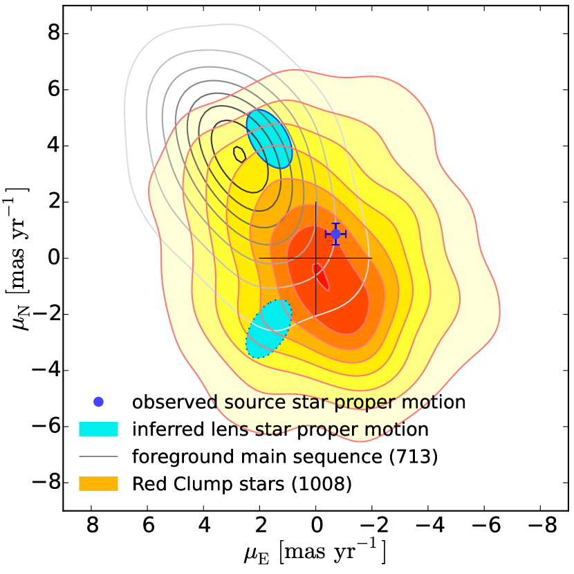
Figure 4: Smoothed proper motion distributions of Galactic-bar red clump (RC) stars and foreground disk main-sequence (MS) stars. The source proper motion ${\mbox{\boldmath$\mu$}}_{s}$ is well-measured (blue point). Combining this with the two microlensing solutions in Table 2 yields two possible estimates for the lens proper motion ${\mbox{\boldmath$\mu$}}_{l}$ (centers of cyan ellipses). The ellipses themselves take account of both the measurement errors entering into the determination of ${\mbox{\boldmath$\mu$}}_{l}$ and the intrinsic proper-motion dispersion of disk lenses. See text for details. The northern and southern ellipses correspond to the $(-,-)$ and $(+,+)$ solutions, respectively.

This discrepancy is related to the fact that, at next order in $q$ (i.e., away from the $q\rightarrow 0$ limit), the $(s\leftrightarrow s^{-1})$ degeneracy is actually trajectory-specific (An, 2005). That is, it becomes a one-dimensional (1-D) degeneracy on a cut through the 2-D magnification plane. See Figure 4 from Albrow et al. (2002) and Figure 8 from Afonso et al. (2000). Hence, when both ground-based and Spitzer data sets are fit jointly to the “wide” solution, they prove incompatible, with $\Delta\chi^{2}=522$ (compared to 2L1S), i.e., 358 higher than the sum of the two $\Delta\chi^{2}$ from the separate fits.

3.2 Seven-Parameter Solutions (Free $\rho$)

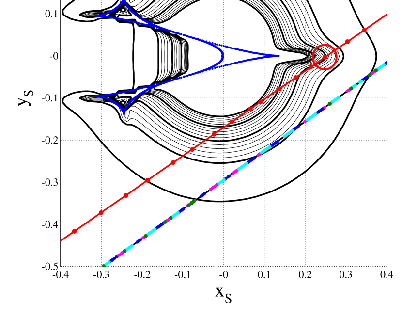
Figure 2: Lens geometry for the “$(+,+)$” 2L1S model of OGLE-2017-BLG-1140. The caustic structure is shown by a closed concave polygon. The point-source magnification contours for $A_{\rm point-source}=(3,4,5,6,7)$ are shown in thick lines, with finer grading shown in thin lines. The two source trajectories (space and ground) are populated by source positions (relative to the lens structure) at the times of observations. These are color-coded by observatory. The source size is shown as an open red circle. This illustrates how the source is resolved by the “magnification ridge” that extends from the cusp along the $x$-axis.

Next, we allow $\rho$ to vary freely in the MCMC, seeded by the Spitzer-only, ground-only, and joint $(+,+)$ solutions from Table 1 The best-fit parameters are shown in Table 2, and the geometry of the joint solution is shown in Figure 2. The “bump” in the Spitzer light curve is caused by the source passing over the ridge extending from a cusp of the central caustic. The ground-based light curve is also affected by this cusp passage, but because the source lies further from the cusp as seen from Earth, its effect on the light curve is not as easily discernible by eye. Nevertheless, as demonstrated by the similarity of the solutions in Tables 1 and 2, the ground-based light curve is sufficiently impacted to measure the planetary parameters.

The geometry shown in Figure 2 is of the so-called “$(+,+)$” solution, i.e., with $u_{0}>0$ for both ground-based and Spitzer observatories. For 1L1S parallaxes, there is a generic four-fold degeneracy corresponding to the four possible sign combinations as seen from Earth and the satellite, i.e., $(+,+)$, $(+,-)$, $(-,+)$, and $(-,-)$. These can also be expressed as $(+,-)\times({\rm same},{\rm opposite})$, where the first component gives the sign of $u_{0}$ as seen from Earth and the second tells whether the satellite $u_{0}$ has the “same” or “opposite” sign. For well-covered binary lenses, we expect that the “$({\rm same},{\rm opposite})$” degeneracy will be broken, although if good coverage is lacking, this degeneracy may persist (Zhu et al., 2015). Figure 2 illustrates this principle very well. We can see that if the Earth trajectory were transposed to the opposite side of the host (but with the same direction), it would be impacted by several cusps and caustics, so that its magnification profile would completely fail to match the observed light curve. Indeed, we confirm by numerical modeling that there are no viable “opposite” [$(+,-)$ and $(-,+)$] solutions. However, there is a competitive $(-,-)$ solution, the parameters of which are given in Table 2. As is often the case (Skowron et al., 2011), these parameters are nearly the same as for $(+,+)$ except for the sign reversals of $(u_{0},\alpha,\pi_{{\rm E},N})$.

Comparing Tables 1 and 2, we see that there is $\Delta\chi^{2}=22.9$ improvement for the $(+,+)$ solution when adding $\rho$ as a free parameter (and $\Delta\chi^{2}=24.9$ for $(-,-)$). The physical origin of this measurement lies in the narrowness of the magnification ridge that extends from the cusp seen in Figure 2, which is of the same order as the normalized source size. This is qualitatively similar to the case of OGLE-2016-BLG-1195Lb (Bond et al., 2017; Shvartzvald et al., 2017). Because $\rho$ is not constrained at all in the ground-only models (see Table 2), one might suspect that the $\chi^{2}$ improvement comes entirely from the Spitzer data. In fact, this is not the case: For the $(+,+)$ solution, only $\Delta\chi^{2}_{spitzer}=11$ comes from Spitzer with the rest coming from the ground. Comparing Tables 1 and 2, we see that the $(s,q)$ values for Spitzer-only and ground-only agree significantly better in the latter than the former. Moreover the $(s,q)$ values of the joint solution in Table 2 are nearly identical to those of the ground-only solution. This means that the ground-only model in Table 1 has been forced away from its “preferred” solution by the necessity to accommodate adjustments in $(s,q)$ that are needed to reconcile the $\rho=0$ model to the Spitzer data. Once $\rho$ is set free in Table 2, the Spitzer-only model comes much closer to the $(s,q)$ preferred by the ground-only model. In brief, the ground-based data acts to “enforce” $(s,q)$, and this indirectly places constraints on $\rho$. This leads to a factor $\sim 2$ reduction in the error on $\rho$ of the joint solution compared to the Spitzer-only solution, despite the fact that the ground-based data contain no direct information about $\rho$.

4 Physical Parameters

Because $\pi_{\rm E}$ and $\rho$ are both measured, it is only necessary to determine $\theta_{*}$ in order to measure the physical properties of the system. We will then obtain $\theta_{\rm E}=\theta_{*}/\rho$ and thereby the lens mass $M$ and lens-source relative parallax $\pi_{\rm rel}$,

$$M={\theta_{\rm E}\over\kappa\pi_{\rm E}},\qquad\pi_{\rm rel}=\theta_{\rm E}\pi_{\rm E}\,,$$ (4)

where $\kappa\equiv{4G/c^{2}{\rm AU}}\simeq 8.144\,\textrm{mas}\,\textrm{M}_{\odot}^{-1}$ (see e.g. Gould (2000) for an introduction to the concepts and formalism of microlensing).

4.1 Information From Microlens Parallax Only

Nevertheless, it is instructive to ask what can be known without the $\theta_{\rm E}$ measurement, particularly because, for the overwhelming majority of the non-planetary “comparison sample” needed to determine the Galactic distribution of planets, $\theta_{\rm E}$ is not measured (Zhu et al., 2017).

We begin by calculating the heliocentric projected velocity for the two solutions in Table 2 (see also Table 3, below),

$$\tilde{\bf v}_{\rm hel}=\tilde{\bf v}_{\rm geo}+{\bf v}_{\oplus,\perp}\equiv{{\rm AU}{\mbox{\boldmath$\pi$}}_{\rm E}\over\pi_{\rm E}^{2}t_{\rm E}}+{\bf v}_{\oplus,\perp}\,,$$ (5)

which, in equatorial coordinates, can be evaluated,

$$\tilde{\bf v}_{\rm hel}(N,E)=\Biggl{[}{(+1031,+719)\atop(-1031,+728)}\Biggr{]}\,{\rm km}\,{\rm s}^{-1}\quad\Biggl{[}{(-,-)\atop(+,+)}\Biggr{]}\,.$$ (6)

Here, ${\bf v}_{\oplus,\perp}=(-0.8,+28.0)\,{\rm km}\,{\rm s}^{-1}$ is the velocity of Earth at the peak of the event, projected onto the plane of the sky. It is notable that the direction of the $(-,-)$ solution (i.e., $35^{\circ}$ north through east) is very similar to the direction of Galactic rotation. This would make it highly compatible with a disk lens. That is, in general,

$$\tilde{\bf v}_{\rm hel}={{\rm AU}\over\pi_{\rm rel}}{\mbox{\boldmath$\mu$}}_{\rm hel}\,,$$ (7)

and so, ignoring the peculiar motions of the source, lens, and Sun, we expect that the projected velocity will lie almost exactly in the direction of Galactic rotation. This is because the Local Standard of Rest (of the Sun) and the local standards of rest of other disk stars both partake of this motion, while the Galactic bar (the presumed home of the source) rotates in very nearly the same direction.

In fact, although this mean motion of the bar is usually ignored (but see Ryu et al. 2017), this is not strictly permissible in the present case because the Galactic longitude $l=4.0$ is relatively high. Applying the Law of Sines and the Exterior Angle Theorem, one finds that for solid body rotation at $\Omega$, the mean source proper motion is given by

$$\langle{\mbox{\boldmath$\mu$}}_{s}\rangle=\sin l(\cos l\cot\psi-\sin l){\mbox{\boldmath$\Omega$}}\rightarrow(\sin l\cot\psi){\mbox{\boldmath$\Omega$}}\,,$$ (8)

where $\psi$ is the bar angle and where we have eliminated second-order terms in the final expression. Adopting $\Omega=75\,{\rm km}\,{\rm s}^{-1}\,{\rm kpc}^{-1}$ and $\psi=40^{\circ}$, we obtain $\langle\mu_{s}\rangle=1.3\,{\rm mas}\,{\rm yr}^{-1}$ for this field. Therefore, for disk lenses we expect

$$\langle{\mbox{\boldmath$\mu$}}_{\rm rel}\rangle={{\bf v}_{\rm rot}\over D_{S}}-(\sin l\cot)\psi{\mbox{\boldmath$\Omega$}}\rightarrow 4.3\,{\rm mas}\,{\rm yr}^{-1}\,{{\bf v}_{\rm rot}\over v_{\rm rot}}\,,$$ (9)

where ${\bf v}_{\rm rot}$ is the velocity of Galactic rotation, $v_{\rm rot}=|{\bf v}_{\rm rot}|\sim 220\,{\rm km}\,{\rm s}^{-1}$, and $D_{S}\sim 8.1\,{\rm kpc}$ (see Section 4.3). Thus, while the direction of the lens-source relative motion of the $(-,-)$ solution (Equation (6)) favors disk lenses, the amplitude of the expected relative proper motion is actually very similar for both disk and bulge lenses.

Next, we insert this estimate of $\mu_{\rm rel}$ for disk lenses and the value of $\tilde{v}$ from Equation (6) to obtain

$$\langle\pi_{\rm rel}\rangle={v_{\rm rot}/D_{S}-(\sin l\cos\psi)\Omega\over\tilde{v}_{\rm hel}}{\rm AU}\rightarrow 0.016\,{\rm mas}\,.$$ (10)

This means that the $(-,-)$ projected velocity is very nearly what would be expected for a disk lens with source-lens separation $D_{LS}\sim 1.0\,{\rm kpc}$. In this case (and taking account of Equation (4)), we should have $\theta_{\rm E}\simeq 0.17\,{\rm mas}$ and so $M=\theta_{\rm E}/\kappa\pi_{\rm E}\simeq 0.22\,M_{\odot}$. On the other hand, both solutions in Equation (6) are quite compatible with the lens being in the bulge, in which case $\pi_{\rm rel}$ would likely be slightly smaller, implying (at fixed $\pi_{\rm E}$), smaller $M$ and $\theta_{\rm E}$ as well.

These arguments imply that, in the absence of any information about $\theta_{\rm E}$ (the typical case for the non-planetary “comparison sample”), the microlens parallax measurement by itself would not discriminate well between bulge and disk lenses. This would not be particularly troubling for the comparison sample because it is used only to construct a comparison cumulative distribution of lens distances, so the role of any particular lens in this relatively large sample is quite minor (Calchi Novati et al., 2015a; Zhu et al., 2017).

However, it also shows that unless the measured lens-source relative proper motion turns out to be unexpectedly low (which would favor a bulge lens), this proper motion measurement is unlikely, by itself, to add to the discriminatory power to what can be determined from the ${\mbox{\boldmath$\pi$}}_{\rm E}$ measurement alone. We return to this point in Section 4.4.

4.2 Color-Magnitude Diagram

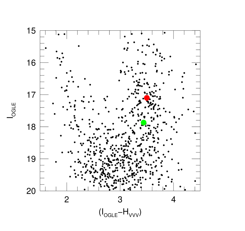
Figure 3: Color-magnitude diagram (CMD) from combining OGLE-IV $I$-band and VVV $H$-band data. The source position (green) in these two bands is determined from the best-fitting model to the OGLE $I$ and SMARTS ANDICAM $H$, with the latter transformed to the VVV system from field stars. The clump centroid is shown in red.

To measure $\theta_{\rm E}=\theta_{*}/\rho$, we evaluate $\theta_{*}$ by placing the source on a color-magnitude diagram (CMD) (Yoo et al., 2004). However, because of high extinction, $V_{s}$ is poorly measured, so we cannot place the source directly on an $[I,(V-I)]$ CMD. Instead we use SMARTS (1.3m) ANDICAM $H$-band data (together with OGLE $I$-band data) to derive $(I_{\rm OGLE-IV}-H_{s,\rm ANDICAM})=-1.21\pm 0.01$ in the instrumental system, by aligning these to the best fit model. We then calibrate this to the much deeper VVV catalog and find $H_{\rm ANDICAM}-H_{\rm VVV}=4.65\pm 0.01$ from field stars. This yields $(I_{\rm OGLE-IV}-H_{s,\rm VVV})=3.44\pm 0.02$. From the fit to the light curve (Table 2), $I_{s,\rm OGLE-IV}=17.86\pm 0.02$. We compare these values to those of the clump on the OGLE-IV/VVV CMD (Figure 3), $[(I-H),I]_{\rm cl}=(3.50,17.10)\pm(0.05,0.08)$, and derive an offset $\Delta[(I-H),I]=(-0.06,+0.76)\pm(0.05,0.08)$. Using the color-color relations of Bessell & Brett (1988), we translate this to an offset $\Delta[(V-I),I]=(-0.04,+0.76)\pm(0.05,0.08)$ on the $V/I$ CMD. We adopt $[(V-I),I]_{0,\rm cl}=(1.06,14.33)$ from Bensby et al. (2013) and Nataf et al. (2013), to finally derive $[(V-I),I]_{0,s}=(1.02,15.09)\pm(0.05,0.08)$. We then convert from $V/I$ to $V/K$ using the color-color relations of Bessell & Brett (1988), with $(V-K)=2.36\pm 0.12$. Finally, we use the Kervella et al. (2004) surface brightness relation to evaluate the angular diameter, $\theta_{\mathrm{LD}}$

$$\log(\theta_{\mathrm{LD}})=0.2672\,(V-K)+0.5354-0.2\,V\,.$$ (11)

The resulting source angular radius is

$$\theta_{*}=4.39\pm 0.38\,\mu{\rm as}\,.$$ (12)

We recall that, within this evaluation, based on the determination of the offset of the source within the CMD to the clump, the CMD itself does not need to be calibrated, specifically zero point offsets cancel out in the calculation. We also recall that the OGLE-IV $I$ bandpass is extremely close to Cousins (Udalski et al., 2015b). In particular the color term is well below the uncertainty of measurement of the clump centroid.

The final error budget for $\theta_{*}$, relative error 8.7%, is dominated by the uncertainty in centroiding the clump and the conversion $(V-I,I)$ to $(V-K,K)$. Specifically, the error in the conversion of $(I-H)$ to $(V-I)$ is about 0.006 mag (this is because the offset from the clump is only 0.06 mag), well below the error in centroiding the clump, and so can be ignored. The relative error would drop to 3.2% if we neglected the error in centroiding the clump and to about 5.4% if we neglected the propagation error from $(V-I)$ to $(V-K)$. Finally, the error in the surface brightness relation is also negligible, with the relative error at the 1% level.

4.3 Evaluation of Physical Parameters

Inserting the measurements of $\rho$ and $t_{\rm E}$ from Table 2, the value in Equation (12) yields

$$\theta_{\rm E}={\theta_{*}\over\rho}=0.16\pm 0.02\,{\rm mas}\,,\qquad\mu_{\rm rel}={\theta_{\rm E}\over t_{\rm E}}=4.1\pm 0.6\,{\rm mas}\,{\rm yr}^{-1}\,.$$ (13)

These values are very similar to those “predicted” in Section 4.1 for a disk lens prior to incorporating information about $\theta_{\rm E}$. As discussed there, this immediately implies that, although the lens distance is well measured, we cannot, on the basis of the microlensing solution alone, strongly discriminate between the lens lying in the disk or the bulge. We return to this problem in Section 4.4.

The simultaneous measurement of both the microlens parallax, $\pi_{\rm E}$, and the Einstein angular radius, $\theta_{\rm E}$, together with that of the microlensing parameter $q=M_{\rm planet}/M_{\rm host}$, finally allow us to determine the physical parameters of the system (Equation (4)). In Table 3 we present the solution, and in particular we find

$$M_{\rm host}=0.21\pm 0.03\,M_{\odot}\,;\qquad M_{\rm planet}=1.6^{+0.4}_{-0.3}\,M_{\rm jup}\,.$$ (14)

Note that in lieu of the lens distance, $D_{L}$, we rather report

$$D_{8.3}\equiv{{\rm kpc}\over 1/8.3+\pi_{\rm rel}/{\rm mas}}\,.$$ (15)

The primary reason for this is that $D_{8.3}$ is much better constrained than $D_{L}$ because the error in the distance to the source (due to the finite depth of the bar) is of the same order as the distance from the lens to the source, $D_{LS}\equiv D_{S}-D_{L}$. Note that for cases like the present one, for which $D_{LS}\ll D_{L}$, we have approximately $D_{LS}\simeq 8.3\,{\rm kpc}-D_{8.3}$. In particular, Calchi Novati et al. (2015a) introduced $D_{8.3}$ in order to put all Spitzer lenses on a homogeneous distance scale with minimal error.

However, we should also note that, at $l=4.0$, the source is fairly far out on the near side of the Galactic bar and that the value of $I_{\rm cl}=14.33$ adopted in Section 4.2 corresponds to a mean distance to the bar of $D_{\rm bar}\sim 7.8\,{\rm kpc}$. If the lens lay well in the foreground of the bar, then this would also be a good mean estimate for $D_{S}$. However, because the lens is either in or near the bar, the mean estimate of the source distance is “pushed back”, simply because the cross section for lensing scales $\sim\sqrt{D_{LS}}$. In particular, if the lens were known to be in the bar, the best estimate of the source distance would be $D_{S}=D_{\rm bar}+D_{LS}/2=8.3\,{\rm kpc}$. A similar effect (but not as strong) applies to disk lenses near the bar, $D_{S}\sim 8.0\,{\rm kpc}$. We adopt $D_{S}\simeq 8.1\,{\rm kpc}$ to evaluate the planet-host projected separation, $a_{\perp}$,

$$a_{\perp}=1.02\pm 0.15\,{\rm AU}\,.$$ (16)

4.4 Source Proper Motion

We are fortunate that the source is a giant star that is relatively bright (despite significant extinction), relatively isolated, and only slightly blended. This means that we can measure the source proper motion ${\mbox{\boldmath$\mu$}}_{s}$, which will enable a much more precise determination of the lens proper motion, ${\mbox{\boldmath$\mu$}}_{l}={\mbox{\boldmath$\mu$}}_{s}+{\mbox{\boldmath$\mu$}}_{\rm rel}$, than would otherwise be possible. This can in principle provide a decisive kinematic discriminant between the bulge-lens and disk-lens interpretations. More specifically, as we will show, certain values of ${\mbox{\boldmath$\mu$}}_{l}$ would decisively rule out disk lenses, but no measured value of ${\mbox{\boldmath$\mu$}}_{l}$ would by itself decisively confirm the lens as belonging to the disk.

The rationale of the present analysis is to compare the estimated lens proper motion to that of the field bulge and main sequence (disk) populations. To estimate the relative probability of a disk versus a bulge lens, going beyond a possible “at glance” analysis from Figure 4, we should take into account both the underlying kinematic and density distributions for both populations. Below we make a detailed evaluation of the relative probability based on the kinematic distributions. On the other hand, the disk and bulge density profiles at the lens distance toward this direction are too poorly understood at present to evaluate the density term of the relative probability. In the next few years we may expect, following the GAIA DR2 release and therefore the knowledge of the astrometry of the bulge as a whole, to understand much better these density profiles. Together with the analysis presented here, this will then allow one to obtain a reliable estimate of bulge-vs-disk lens.

We begin by identifying three sets of stars from a color-magnitude diagram of stars in a $6.5^{\prime}$ square centered on the event: 1008 bulge red clump (RC) stars, 2123 bulge red giant branch (RGB) stars, and 713 foreground main-sequence (MS) stars. We measure the vector proper motions of each star (relative to a frame set by the RC stars) based on 250 (out of 708) better-seeing ($0.9^{\prime\prime}<{\rm FWHM}<1.3^{\prime\prime}$) OGLE-IV images from $5275.9\leq{\rm HJD}^{\prime}\leq 8019.6$. The typical proper motion errors (derived from internal scatter) are $\sigma_{\mu}\sim 0.5\,{\rm mas}\,{\rm yr}^{-1}$. We exclude a handful of stars with individual errors $\sigma>2\,{\rm mas}\,{\rm yr}^{-1}$. (The numbers given above already take account of this exclusion.)  Figure 4 shows contours of the RC and MS proper motion distributions based on smoothed counts, and also shows the proper motion of the source star:

$${\mbox{\boldmath$\mu$}}_{s}(N,E)=(0.86,-0.71)\pm(0.38,0.36)\,{\rm mas}\,{\rm yr}^{-1}\,.$$ (17)

Figure 4 also shows the lens proper motion ${\mbox{\boldmath$\mu$}}_{l}$ together with an error ellipse (defined by covariance matrix $c_{ij}$, which we describe further below),

$${\mbox{\boldmath$\mu$}}_{l}(N,E)=(4.21,1.63)\,{\rm mas}\,{\rm yr}^{-1};\qquad c_{ij}=(1.10,0.42,0.42,0.67),({\rm mas}\,{\rm yr}^{-1})^{2}\,,$$ (18)

where we have included the very small $(<0.1\,{\rm mas}\,{\rm yr}^{-1})$ correction from geocentric to heliocentric proper motion.

From Figure 4, one sees that the lens proper motion is offset from the peak of the MS distribution by

$$\Delta{\mbox{\boldmath$\mu$}}(N,E)={\mbox{\boldmath$\mu$}}_{l}-{\mbox{\boldmath$\mu$}}_{\rm peak-MS}=(0.56,-0.89)\,{\rm mas}\,{\rm yr}^{-1}\,,$$ (19)

where ${\mbox{\boldmath$\mu$}}_{\rm peak-MS}(N,E)=(3.65,2.52)\,{\rm mas}\,{\rm yr}^{-1}$ is the peak of the MS distribution. To assess the level of consistency represented by this offset, we consider three sources of uncertainty. Two of these are error terms related to the measurement of ${\mbox{\boldmath$\mu$}}_{l}={\mbox{\boldmath$\mu$}}_{s}+\hat{\bf n}\mu_{\rm rel}$, where $\hat{\bf n}\equiv{\mbox{\boldmath$\mu$}}_{\rm rel}/\mu_{\rm rel}$ is the direction of ${\mbox{\boldmath$\mu$}}_{\rm rel}$, i.e., the same as the direction of $\tilde{\bf v}$. From Equation (17), the first-term covariance matrix is almost isotropic. On the other hand, because $\hat{\bf n}$ is measured extremely well (see Table 2), the covariance matrix associated with ${\mbox{\boldmath$\mu$}}_{\rm rel}$ is nearly degenerate. Adding these two, we find $c^{\rm meas}_{ij}=(0.35,0.14,0.14,0.23)\,({\rm mas}\,{\rm yr}^{-1})^{2}$.

The third source of uncertainty relates to the prediction of the lens proper motion under the assumption that the lens is in the disk. We assume that the velocity dispersion of the lenses is $(33,18)\,{\rm km}\,{\rm s}^{-1}$ in the rotational and vertical directions, i.e., similar to local disk stars. We then rotate to equatorial coordinates to obtain a covariance matrix $c^{\rm pred}_{ij}=(0.75,0.28,0.28,0.43)\,({\rm mas}\,{\rm yr}^{-1})^{2}$. We can then evaluate the $\chi^{2}$ of the measured offset $\Delta{\mbox{\boldmath$\mu$}}$ given these uncertainties

$$\chi_{\rm offset}^{2}=\sum_{ij}b_{ij}(\Delta\mu)_{i}(\Delta\mu)_{j}=2.72;\qquad b\equiv c^{-1};\qquad c_{ij}=c_{ij}^{\rm meas}+c_{ij}^{\rm pred}\,;$$ (20)

For a 2-D Gaussian, this has probability $P(\chi^{2}_{\rm offset})=\exp(-\chi^{2}/2)=0.26$ which is quite reasonable. From Figure 4, it is clear that the great majority of stars drawn randomly from the bulge population would have dramatically lower $P$ values.

We note that, properly speaking, the $c^{\rm meas}_{ij}$ ellipse should be drawn around ${\mbox{\boldmath$\mu$}}_{l}$ while the $c^{\rm pred}_{ij}$ ellipse should be drawn around ${\mbox{\boldmath$\mu$}}_{\rm peak-MS}$. However, we have combined the two covariance matrices (Equation (20)) for three reasons. First, from a mathematical standpoint, Equation (20) remains valid regardless of whether the contributing covariance matrices are summed before or after display. Second, with this display, the level of discrepancy is directly manifest in the diagram. Third, this mode of display will facilitate numerical evaluations below.

We also show a second error ellipse in the lower part of Figure 4. Any lens star that actually lay in this ellipse would (due to the $(+,+)\leftrightarrow(-,-)$ degeneracy: see Table 2) produce the same solutions as a corresponding star in the upper ellipse. Hence, the two groups of potential lenses can only be distinguished at the $1\,\sigma$ level, and so must both be considered.

Assuming that the proper motions of lenses and sources are independent of their distances within the narrow limits permitted by the microlensing solution (a point to which we return below), the relative probability of a disk versus bulge lens can be factored,

$${P_{\rm disk}\over P_{\rm bulge}}=\biggl{(}{P^{\rm kin}_{\rm disk}\over P^{\rm kin}_{\rm bulge}}\biggr{)}\biggl{(}{P^{dens}_{\rm disk}\over P^{\rm dens}_{\rm bulge}}\biggr{)};\qquad{P^{\rm kin}_{\rm disk}\over P^{\rm kin}_{\rm bulge}}={f^{(-,-)}_{\rm disk}+Qf^{(+,+)}_{\rm disk}\over f^{(-,-)}_{\rm bulge}+Qf^{(+,+)}_{\rm bulge}}\,,$$ (21)

where $f_{\rm disk}({\mbox{\boldmath$\mu$}}_{l})$ and $f_{\rm bulge}({\mbox{\boldmath$\mu$}}_{l})$ are the normalized proper motion distributions of the disk and bulge populations respectively (convolved with measurement errors, as above), $f^{(-,-)}$ and $f^{(+,+)}$ are values of these distribution at the measured values of the two solutions, and $Q\equiv\exp(-(\chi^{2}_{{\rm mod}(+,+)}-\chi^{2}_{{\rm mod}(-,-)})/2)=0.61$ is the relative likelihood of the microlensing models based on the $\chi^{2}$ values in Table 2. We focus here on the first (kinematic) term, which is written more explicitly in the second expression of Equation (21).

As we describe below, the values of $f^{(-,-)}_{\rm bulge}$ and $f^{(+,+)}_{\rm bulge}$ can be evaluated purely empirically by counting RC (or RGB) stars in small areas in the neighborhoods of the two solutions and comparing these values to the total sample. However, the same principle cannot be applied to find $f^{(-,-)}_{\rm disk}$ and $f^{(+,+)}_{\rm disk}$ by counting MS stars. This is because the MS stars come from many different distances $D$ along the line of sight. If, as in many Galactic models used to carry out Bayesian analyses (e.g., Han & Gould 1995), the rotation curve is assumed flat, then the mean proper motion of disk stars at any distance will always be the same. For this reason, it is appropriate to use the peak of the observed MS proper motions to evaluate the mean proper motion of disk stars at the distance of the lens, $D_{L}$. However, if (as also usually assumed) the velocity dispersions are independent of distance, then the proper-motion dispersions of disk stars scale $\sigma(\mu)\propto D^{-1}$. Since disk stars that are closer are systematically brighter at fixed luminosity (due both to proximity and lower extinction), the sample of MS stars is highly biased toward nearby stars with larger proper-motion dispersions that are quite unrepresentative of stars at $D_{L}\sim 7\,{\rm kpc}$. It is for this reason that we evaluated $c_{ij}$, including both intrinsic dispersion and measurement errors. Therefore, we can write

$$P^{\rm kin}_{\rm disk}=f^{(-,-)}_{\rm disk}+Qf^{(+,+)}_{\rm disk}={\exp(-\chi^{2}_{\rm offset}/2)\over 2\pi\sqrt{|c|}}+Q{\exp(-\chi^{2}_{{\rm offset},(+,+)}/2)\over 2\pi\sqrt{|c^{(+,+)}|}}\rightarrow{\exp(-\chi^{2}_{\rm offset}/2)\over 2\pi\sqrt{|c|}}$$ (22)

where we have dropped the second term in the final expression because $\chi^{2}_{{\rm offset},(+,+)}=55$. Noting that $\pi|c|^{1/2}$ is just the area of the error ellipse, we can now express the ratio of kinematic probabilities as

$${P^{\rm kin}_{\rm disk}\over P^{\rm kin}_{\rm bulge}}={\exp(-\chi^{2}_{\rm offset}/2)/2\over(N_{\rm bulge}^{(-,-)}+QN_{\rm bulge}^{(+,+)})/N_{\rm bulge}}\rightarrow 3.0\pm 0.3\,,$$ (23)

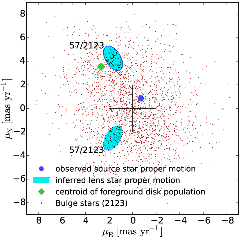
Figure 5: Observed proper motions of bulge red giant branch (RGB) stars in a $6.5^{\prime}$ square around OGLE-2017-BLG-1140. The cyan ellipses are the same as in Figure 4. The fractions of RGB stars that lie in each ellipse (57/2123 in both cases) enter the estimate of relative kinematic probability of disk versus bulge lenses. See Equation (23).

where we have made the evaluation using the RGB sample with $N_{\rm bulge}=2123$, and where $N_{\rm bulge}^{(-,-)}=57$ and $N_{\rm bulge}^{(+,+)}=57$ are the numbers of RGB stars in the two ellipses shown in Figure 5.

Before continuing, we note that we performed a similar test, but restricted to the 1008 RC stars, which are basically a subset of the RGB sample, but even less prone to contamination from foreground disk stars. We found 23 and 36 stars in the $(-,-)$ and $(+,+)$ ellipses. Inserting these numbers into Equation (23) we obtain $P^{\rm kin}_{\rm disk}/P^{\rm kin}_{\rm bulge}=2.9\pm 0.4$., which (even considering that these are overlapping samples) is consistent at the $1\,\sigma$ level. Given that the sign of the difference is the opposite of what one would expect from greater contamination of the RGB sample, we adopt the RGB value (i.e., Equation (23)).

A more detailed analysis would require a more precise Galactic model than presently exists. Below, we outline some of the issues that would have to be addressed by such a model, but the key point is that vastly improved models are likely to be available within a year based on the Gaia DR2 data release. Hence, given the delicacy of the required calculations, it is premature to carry them out based on current Galactic models.

Here, we just illustrate some of the issues that need to be considered. The first issue is that the assumption of constant velocity dispersion may well be incorrect. The scale heights of edge-on disks of external galaxies appear to be constant as a function of radius, while the radial density profiles are eponymously “exponential”. These simple observations argue for a vertical velocity dispersion that scales roughly as the square root of surface density. However, by chance, any such adjustment would have a small effect in the present case. To see this, first note that (again by chance), $c_{ij}^{\rm pred}\simeq 2c_{ij}^{\rm meas}$. Therefore, if we were to, say, double the dispersions (i.e., multiply $c_{ij}^{\rm pred}$ by a factor four), this would increase $c$ by a factor 3.0. This would then change $P_{\rm disk}^{\rm kin}$ by a factor: $\exp(\chi^{2}_{\rm offset}/3)/3=0.83$.

A second kinematic issue arises from possible streaming motions along the bar, which might for example be responsible for the elongated contours along the direction of the Galactic plane in the RC distribution shown in Figure 4. The lens must be in front of the source (by $D_{LS}\sim 1\,{\rm kpc}$). Hence, if this streaming motion were primarily “outward” for stars in the closer side of the bar, then there would be a relatively big population of potential bulge lenses with proper motions strongly aligned with Galactic rotation. On the other hand, if the outward streaming motion were mainly on the more distant side of the bar (and the nearer side was streaming toward the Galactic center), then a bulge lens would be much less likely.

Finally, the density distribution of both the bar and the disk in this region must be estimated much more precisely than at present. For example, a very narrow bar would make it difficult to accommodate both a lens and source, with $D_{LS}\sim 1\,{\rm kpc}$. Moreover, it is possible that the disk in the immediate neighborhood of the bar is depleted relative to an exponential profile, due to action by the bar.

For these reasons, we defer a detailed calculation of $P_{\rm disk}/P_{\rm bulge}$ until more precise models are developed on the basis of the Gaia DR2 release.

5 A New Approach to Breaking the 2L1S/1L2S Degeneracy

The space-based and ground-based light curves are each reasonably well fit to 1L2S models. These models have six non-linear parameters, $[(t_{0},u_{0})_{1,2},t_{\rm E},q_{f}]$. Because there are two sources, there are two pairs of $(t_{0},u_{0})$, one for each source. The flux ratio $q_{f}$ is assumed to be the same for all observations in the same band (in our case $I$ for ground-based data and $L$ for Spitzer data). For fits with more than one band, there is one “$q_{f}$” for each band. Table 4 shows the fit parameters for Spitzer-only, ground-only, and joint 1L2S fits.

Comparing the $\chi^{2}$ values to those in Table 2, we see that $\Delta\chi^{2}\equiv\chi^{2}({\rm 1L2S})-\chi^{2}({\rm 2L1S})$ takes on values $\Delta\chi^{2}=(+55,+19,+804)$ for Spitzer-only, ground-only, and Spitzer+ground data sets, respectively. That is, whereas the 2L1S and 1L2S geometries yield models with qualitatively comparable $\chi^{2}$ values when the ground-based data are analyzed alone, and are moderately-well distinguished based on Spitzer data alone, the 1L2S solution is decisively excluded for the joint fit to all data.

As a first step toward understanding the physical origin of this effect, we note that whereas for 2L1S, $\chi^{2}_{\rm joint,2L1S}=\chi^{2}_{spitzer,\rm 2L1S}+\chi^{2}_{\rm ground,2L1S}-2$, for 1L2S we find $\chi^{2}_{\rm joint,1L2S}=\chi^{2}_{spitzer,\rm 1L2S}+\chi^{2}_{\rm ground,1L2S}+725$. The approximate equality, $\chi^{2}_{\rm joint,2L1S}\simeq\chi^{2}_{spitzer,\rm 2L1S}+\chi^{2}_{\rm ground,2L1S}$, is expected from the fact (already noted in Section 3.1) that the Spitzer-only and ground-only 2L1S solutions are compatible with each other. This leads us to investigate whether the analogous 1L2S solutions are incompatible with each other.

To pursue this question further, we introduce for 1L2S models the vector offset within the Einstein ring of the two sources,

$$(\Delta\tau,\Delta\beta)_{\rm 1L2S}\equiv\biggl{(}{t_{0,2}-t_{0,1}\over t_{\rm E}},u_{0,2}-u_{0,1}\biggr{)}\,.$$ (24)

Ignoring the very small motion of the binary source during the few days between the passage of the lens by the sources, these vector offsets should be the same as seen by two different observers. However, we find from Table 4,

$$(\Delta\tau,\Delta\beta)_{\rm ground,1L2S}=(+0.31,+0.15);\qquad(\Delta\tau,\Delta\beta)_{spitzer,\rm 1L2S}=(+0.19,+0.09)\,.$$ (25)

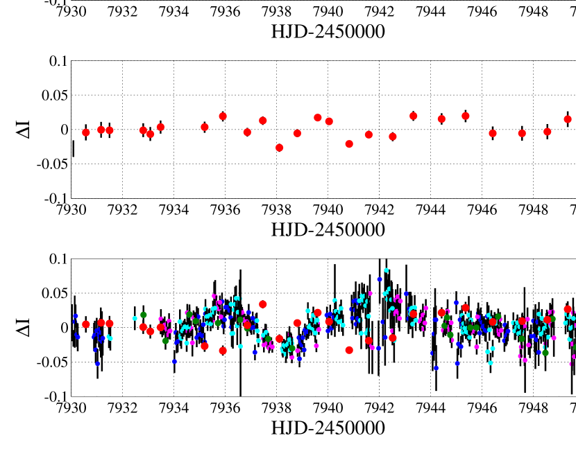
Figure 6: Residuals to single-lens/binary source (1L2S) models for three cases: ground-only, Spitzer-only, and joint fits to all of the data. While the residuals shown in the upper two panels are somewhat worse than those shown for the 2L1S case in Figure 1, the residuals for the joint fit (bottom panel) are dramatically worse. This is because the separate solutions are consistent with each other for 2L1S, but not for 1L2S. See Section 5.

In particular, we note that the offsets in $t_{0}$ differ by about 1.7 days between models of the two data sets, whereas the errors in the individual measured values are all less than 0.04 days. Hence, in the joint solution, the two separately-successful 1L2S models cannot be accommodated with a single $(\Delta\tau,\Delta\beta)_{\rm 1L2S}$. This inconsistency is illustrated by the residuals to the three fits, which are shown in Figure 6.

The fundamental origin for this incompatibility is that the magnification (actually, logarithm of magnification) falls off at different rates for binary-lens (or multi-lens) cusps than it does for point lenses. Of course, it is possible to arrange special geometries that avoid this problem. For example, if the impact parameter is the same as seen by the two observatories, so that the same event essentially repeats at a later time, which can occasionally happen (Udalski et al., 2015a), then any 1L2S/2L1S degeneracy (or indeed any other degeneracy) will persist. However, in the more generic case, we should expect that this degeneracy can be broken provided that both observatories have some sensitivity to both bumps.

6 Discussion

OGLE-2017-BLG-1140 is the first anomalous microlensing event for which observation of the anomaly from both Earth and Spitzer was essential to the proper characterization of the anomaly. In particular, we showed that only by combining both data sets was it possible to decisively discriminate between the 2L1S and 1L2S interpretations. If this indeed represents a new path toward breaking this degeneracy, why is it appearing here for the first time?

For randomly selected microlensing events observed from two platforms, the relative strength of the anomalies observable at the two sites should be likewise randomly distributed. However, among the 18 published 2L1S events observed by Spitzer, OGLE-2017-BLG-1140 is only the second one for which the anomaly was stronger as observed by Spitzer than from the ground. In the other case, OGLE-2017-BLG-1130 (which coincidentally was alerted by OGLE and chosen as a “secret” Spitzer target at exactly the same times as OGLE-2017-BLG-1140), the anomaly was seen from Spitzer only (Wang et al., 2018).

There are four factors that explain this apparent discrepancy. First, of the 18 2L1S events, five had short timescale anomalies due to a planet. Because Spitzer’s cadence has typically been $\Gamma\sim 1\,{\rm day}^{-1}$, it cannot in general be expected to characterize short-term anomalies in the absence of dense ground-based data over the anomaly. That said, it should be pointed out that OGLE-2017-BLG-1140 is one of these five events.

Second, the majority of Spitzer targets are near peak or have already peaked as seen from the ground at the time of the onset of Spitzer observations. This alone would imply that half or more of the anomalies that would be visible from Spitzer’s location are in fact missed by Spitzer observations. This late onset follows from the delay in Spitzer uploads (see Figure 1 of Udalski et al. 2015a) and the difficulty of recognizing and reliably choosing microlensing events based on their early evolution.

Third, due to the direction of Galactic rotation expressed in equatorial coordinates, more disk lenses are traveling east than west, meaning that they peak later as seen from Spitzer, which lies to the west of Earth. In itself, this is a relatively minor effect, but it exacerbates the previous one.

Fourth, Spitzer can observe targets that are near the ecliptic for a maximum of 38 days. Hence, for long events, anomalies can take place outside of the Spitzer window.

Taken together, these four effects mean that the new channel for resolving the 2L1S/1L2S degeneracy will not appear on a routine basis in Spitzer microlensing events. Nevertheless, it is worth noting that despite the relatively weak appearance of the OGLE-2017-BLG-1140 anomaly in ground-based data, the addition of the also fairly modest signal from the Spitzer anomaly dramatically improved the confidence of the result. Further, although the anomaly was recognized in ground-based data soon after it occurred, the event was not systematically analyzed because it appeared to have insurmountable degeneracies. Therefore, it is quite possible that other archival events with even weaker, less noticeable, anomalies can also yield interesting, unexpected results. Moreover, this same principle can be applied to future parallax-satellite missions, including WFIRST (Spergel et al., 2013) as well as other missions that are yet unplanned.

7 Conclusions

We have presented OGLE-2017-BLG-1140Lb, a microlensing extrasolar planet detected combining ground-based survey, OGLE and KMTNet, and space-based, Spitzer, data. From the modeling point of view this event is of particular interest. For the first time Spitzer, besides providing the measure of the microlensing parallax, is essential for the characterization of the planetary system. Indeed, a deviation from the single-lens single-source (1L1S) Paczyński shape is apparent both from ground (specifically, KMTNet), and space-based data which however, separately, are each reasonably well fit by either a single-lens binary-source (1L2S) or a binary-lens single-source (2L1S), planetary, model. The analysis then leads us to show how the microlensing parallax opens a new path for breaking this classic degeneracy (Gaudi, 1998) when combining ground and space-based data. Specifically, we find that that the 1L2S solution is ruled out by $\Delta\chi^{2}\sim 800$ by the combined space/ground analysis, which is a factor 10 higher than the $\Delta\chi^{2}\sim 80$ from the sum of the ground and space analyses considered separately. As for the 2L1S planetary model, the system can be indipendently characterized by Spitzer, whose trajectory passes closer to the caustic structure, and ground-based data, leading roughly to the same configuration (except that ground-based data alone do not allow to constrain the finite source effect parameter, $\rho$). As we show, however, the combination of the two data sets puts a stronger constraint on the caustic structure (the binary parameter $(s,q)$, i.e., the projected separation of the two lenses and their mass ratio, resulting specifically in a “resonant” configuration) and indirectly also on $\rho$. The measurement of $\rho$, together with the photometric characterization of the source, and the measurement of the microlens parallax allow us to determine the physical parameters of the system. Specifically we find $M_{\rm host}=0.21\pm 0.03\,M_{\odot}$ and $M_{\rm planet}=1.6^{+0.4}_{-0.3}\,M_{\rm jup}$, for a lens-to-source distance $D_{LS}\simeq 1\,$kpc, and a planet-host separation $a_{\perp}=1.02\pm 0.15\,{\rm AU}$, well beyond the system snow line. We show that the lens proper motion analysis is consistent with the lens lying in the Galactic disk, although a Bulge lens is not ruled out. In the framework of the Spitzer microlensing survey, OGLE-2017-BLG-1140Lb is the fifth planet to enter the sample for the determination of the Galactic distribution of exoplanets (Calchi Novati et al., 2015a; Zhu et al., 2017).

The discovery of OGLE-2017-BLG-1140Lb, a super-Jupiter mass planet orbiting a M-dwarf (beyond the system snow line), is also relevant in the larger framework of the microlensing statistical census of exoplanets (e.g., Gaudi 2012; Gould 2016). Indeed, out of 58 (microlensing) planets currently known, 11 belong to that same class (specifically for a host mass $0.08<M/M_{\odot}<0.5$, and a planet mass larger than that of Jupiter, e.g., Shvartzvald et al. 2014). OGLE-2017-BLG-1140Lb adds to this sample, and it is the fifth one belonging to the subsample of those with microlens-parallax-based mass measurements, which are substantially more accurate. Notwithstanding the microlensing observational bias for the detection of such planetary systems (e.g., Batista et al. 2011), because of the abudance of M-dwarf and of the detection efficiency’s increase with $q$, the abundance of these systems, about 20% of all microlensing planets, remains a challenge for current planet formation theories (e.g., D’Angelo et al. 2010).

Table 1: 2L1S Solutions with $\rho=0$

Parameter	Spitzer	Ground	Spitzer and ground
$\chi^{2}$/dof	44.8/35	2964.6/2936	3024.9/2975	3025.9/2975
			$(+,+)$	$(-,-)$
$t_{0}$ [HJD-2457940.]	$-0.201_{-0.011}^{+0.011}$	$0.7645_{-0.0066}^{+0.0063}$	$0.7604_{-0.0062}^{+0.0060}$	$0.7606_{-0.0062}^{+0.0061}$
$u_{0}$	$0.1343_{-0.0082}^{+0.0083}$	$0.2373_{-0.0055}^{+0.0044}$	$0.2364_{-0.0042}^{+0.0040}$	$-0.2365_{-0.0040}^{+0.0042}$
$t_{\mathrm{E}}$ [days]	$14.58_{-0.63}^{+0.68}$	$14.74_{-0.13}^{+0.17}$	$14.74_{-0.13}^{+0.14}$	$14.74_{-0.13}^{+0.14}$
$\rho$	0	0	0	0
$\pi_{\mathrm{E,N}}$	-	-	$-0.0793_{-0.0016}^{+0.0016}$	$0.0799_{-0.0016}^{+0.0016}$
$\pi_{\mathrm{E,E}}$	-	-	$0.0524_{-0.0007}^{+0.0007}$	$0.0520_{-0.0007}^{+0.0007}$
$\alpha$ [rad]	$2.561_{-0.013}^{+0.013}$	$2.545_{-0.011}^{+0.012}$	$2.5463_{-0.0083}^{+0.0085}$	$-2.5462_{-0.0083}^{+0.0082}$
$s$	$0.815_{-0.021}^{+0.019}$	$0.855_{-0.019}^{+0.017}$	$0.831_{-0.012}^{+0.012}$	$0.831_{-0.012}^{+0.012}$
$q$	$0.0099_{-0.0013}^{+0.0015}$	$0.0079_{-0.0010}^{+0.0012}$	$0.0090_{-0.0008}^{+0.0009}$	$0.0090_{-0.0008}^{+0.0009}$
$f_{\mathrm{s,OGLE}}$	-	$1.131\pm 0.024$	$1.127\pm 0.020$	$1.127\pm 0.020$
$f_{\mathrm{b,OGLE}}$	-	$0.237\pm 0.024$	$0.241\pm 0.020$	$0.241\pm 0.020$
$f_{\mathrm{s},Spitzer}$	$17.4\pm 1.1$	-	$17.4\pm 0.3$	$17.4\pm 0.3$
$f_{\mathrm{b},Spitzer}$	$2.4\pm 0.9$	-	$2.4\pm 0.3$	$2.5\pm 0.3$
$I-L$	-	-	$2.971\pm 0.007$	$2.971\pm 0.007$

Table 2: 2L1S Solutions with $\rho\neq 0$

Parameter	Spitzer	Ground	Spitzer and ground
$\chi^{2}$/dof	39.4/34	2964.0/2935	3002.0/2974	3001.0/2974
			$(+,+)$	$(-,-)$
$t_{0}$ [HJD-2457940.]	$-0.195_{-0.010}^{+0.010}$	$0.7677_{-0.0066}^{+0.0065}$	$0.7698_{-0.0059}^{+0.0059}$	$0.7701_{-0.0058}^{+0.0059}$
$u_{0}$	$0.1390_{-0.0082}^{+0.0085}$	$0.2395_{-0.0055}^{+0.0040}$	$0.2389_{-0.0040}^{+0.0034}$	$-0.2392_{-0.0032}^{+0.0038}$
$t_{\mathrm{E}}$ [days]	$14.38_{-0.61}^{+0.65}$	$14.68_{-0.11}^{+0.17}$	$14.70_{-0.11}^{+0.14}$	$14.69_{-0.11}^{+0.13}$
$\rho$	$0.0241_{-0.0078}^{+0.0058}$	-	$0.0269_{-0.0034}^{+0.0026}$	$0.0270_{-0.0027}^{+0.0024}$
$\pi_{\mathrm{E,N}}$	-	-	$-0.0782_{-0.0015}^{+0.0016}$	$0.0789_{-0.0015}^{+0.0014}$
$\pi_{\mathrm{E,E}}$	-	-	$0.0531_{-0.0008}^{+0.0007}$	$0.0528_{-0.0007}^{+0.0007}$
$\alpha$ [rad]	$2.557_{-0.012}^{+0.011}$	$2.540_{-0.011}^{+0.012}$	$2.539_{-0.0074}^{+0.0076}$	$-2.5388_{-0.0069}^{+0.0067}$
$s$	$0.857_{-0.028}^{+0.027}$	$0.871_{-0.022}^{+0.026}$	$0.870_{-0.014}^{+0.014}$	$0.871_{-0.013}^{+0.012}$
$q$	$0.0080_{-0.0012}^{+0.0014}$	$0.0072_{-0.0011}^{+0.0012}$	$0.0073_{-0.0007}^{+0.0008}$	$0.0072_{-0.0006}^{+0.0007}$
$f_{\mathrm{s,OGLE}}$	-	$1.138\pm 0.024$	$1.136\pm 0.019$	$1.138\pm 0.018$
$f_{\mathrm{b,OGLE}}$	-	$0.231\pm 0.024$	$0.232\pm 0.019$	$0.231\pm 0.018$
$f_{\mathrm{s},Spitzer}$	$17.9\pm 1.1$	-	$17.7\pm 0.3$	$17.7\pm 0.3$
$f_{\mathrm{b},Spitzer}$	$1.9\pm 1.0$	-	$2.0\pm 0.3$	$2.0\pm 0.3$
$I-L$	-	-	$2.982\pm 0.008$	$2.980\pm 0.007$

Table 3: Physical parameters

Parameter	$(+,+)$	$(-,-)$
$M_{\mathrm{host}}$ ($\mathrm{M}_{\odot}$)	$0.213_{-0.027}^{+0.036}$	$0.211_{-0.025}^{+0.032}$
$M_{\mathrm{planet}}$ ($\mathrm{M}_{\mathrm{Jup}}$)	$1.62_{-0.29}^{+0.41}$	$1.59_{-0.26}^{+0.35}$
$D_{8.3}$ (kpc)	$7.36_{-0.14}^{+0.11}$	$7.36_{-0.12}^{+0.10}$
$\theta_{\mathrm{E}}$ (mas)	$0.164_{-0.020}^{+0.028}$	$0.163_{-0.019}^{+0.024}$
$\pi_{\mathrm{E}}$	$0.0946_{-0.0016}^{+0.0014}$	$0.0949_{-0.0015}^{+0.0014}$
$\pi_{\mathrm{rel}}$ (mas)	$0.0155_{-0.0019}^{+0.0027}$	$0.0154_{-0.0019}^{+0.0023}$
$\mu_{\mathrm{rel}}$ (mas yr-1)	$4.07_{-0.50}^{+0.69}$	$4.04_{-0.48}^{+0.60}$
${\tilde{v}}_{\mathrm{hel,N}}$ (km s-1)	$-1030.7_{-8.7}^{+8.4}$	$1030.9_{-8.2}^{+8.3}$
${\tilde{v}}_{\mathrm{hel,E}}$ (km s-1)	$728_{-13}^{+13}$	$719_{-13}^{+13}$

Table 4: 1L2S Solutions

Parameter	Spitzer	Ground	Spitzer and ground
$\chi^{2}$/dof	94.2/35	2985.3/2936	3834.8/2975	3804.9/2975
			$(+,+)$	$(+,-)$
$t_{\mathrm{E}}$ [days]	$16.06_{-0.74}^{+0.81}$	$15.12_{-0.15}^{+0.15}$	$13.96_{-0.14}^{+0.14}$	$14.49_{-0.17}^{+0.17}$
$t_{0,1}$ [HJD-2457900.]	$37.022_{-0.023}^{+0.023}$	$36.337_{-0.038}^{+0.040}$	$37.698_{-0.031}^{+0.031}$	$38.163_{-0.058}^{+0.057}$
$t_{0,2}$ [HJD-2457900.]	$40.064_{-0.016}^{+0.017}$	$41.026_{-0.019}^{+0.019}$	$40.979_{-0.025}^{+0.025}$	$41.361_{-0.047}^{+0.046}$
$u_{0,1}$	$0.0299_{-0.0027}^{+0.0027}$	$0.0847_{-0.0048}^{+0.0050}$	$0.1808_{-0.0037}^{+0.0039}$	$0.2810_{-0.0081}^{+0.0088}$
$u_{0,2}$	$0.1237_{-0.0073}^{+0.0074}$	$0.2309_{-0.0041}^{+0.0041}$	$0.2752_{-0.0046}^{+0.0048}$	$0.2282_{-0.0054}^{+0.0057}$
$q_{f,I}$	-	$29.5_{-3.0}^{+3.3}$	$15.6_{-1.5}^{+1.7}$	$2.75_{-0.20}^{+0.23}$
$q_{f,L}$	$19.7_{-1.8}^{+2.1}$	-	$12.5_{-1.0}^{+1.0}$	$8.62_{-0.61}^{+0.70}$
$\pi_{\mathrm{E,N}}$	-	-	$-0.1036_{-0.0023}^{+0.0021}$	$-0.2795_{-0.0061}^{+0.0058}$
$\pi_{\mathrm{E,E}}$	-	-	$0.0500_{-0.0012}^{+0.0012}$	$0.0600_{-0.0021}^{+0.0021}$
$\Delta\tau_{\mathrm{Ground}}$	-	$0.3099_{-0.0038}^{+0.0038}$	$0.2355_{-0.0025}^{+0.0025}$	$0.2209_{-0.0034}^{+0.0034}$
$\Delta\tau_{Spitzer}$	$0.1894_{-0.0092}^{+0.0092}$	-	$0.2342_{-0.0026}^{+0.0026}$	$0.2138_{-0.0031}^{+0.0031}$
${\Delta}u_{0,\mathrm{Ground}}$	-	$0.1462_{-0.0072}^{+0.0072}$	$0.0944_{-0.0044}^{+0.0044}$	$-0.531_{-0.0043}^{+0.0043}$
${\Delta}u_{0,Spitzer}$	$0.0939_{-0.0067}^{+0.0067}$	-	$0.0892_{-0.0044}^{+0.0044}$	$0.0666_{-0.0045}^{+0.0045}$
$t_{0,1,Spitzer}$ [HJD-2457900.]	-	-	$36.865_{-0.030}^{+0.030}$	$37.075_{-0.028}^{+0.028}$
$t_{0,2,Spitzer}$ [HJD-2457900.]	-	-	$40.136_{-0.017}^{+0.017}$	$40.172_{-0.017}^{+0.017}$
$u_{0,1,Spitzer}$	-	-	$0.0523_{-0.0028}^{+0.0028}$	$0.0663_{-0.0032}^{+0.0032}$
$u_{0,2,Spitzer}$	-	-	$0.1415_{-0.0025}^{+0.0025}$	$0.1329_{-0.0025}^{+0.0025}$
$f_{\mathrm{s,OGLE}}$	-	$1.069\pm 0.021$	$1.286\pm 0.026$	$1.172\pm 0.029$
$f_{\mathrm{b,OGLE}}$	-	$0.299\pm 0.021$	$0.082\pm 0.026$	$0.195\pm 0.029$
$f_{\mathrm{s},Spitzer}$	$15.3\pm 1.0$	-	$18.0\pm 0.3$	$17.0\pm 0.3$
$f_{\mathrm{b},Spitzer}$	$4.2\pm 0.7$	-	$2.3\pm 0.3$	$3.2\pm 0.3$

References

- Alard & Lupton (1998) Alard, C. & Lupton, R.H.,1998, ApJ, 503, 325
- Albrow et al. (2002) Albrow, M.D., An, J., Beaulieu, J.-P., et al. 2002, ApJ, 572, 1031
- Afonso et al. (2000) Afonso, C., Alard, C., Albert, J.N., et al. 2000, ApJ, 532, 340
- Albrow et al. (2009) Albrow, M. D., Horne, K., Bramich, D. M., et al. 2009, MNRAS, 397, 2099
- An (2005) An, J.H., MNRAS, 356, 1409
- Batista et al. (2011) Batista, V., Gould, A., Dieters, S. et al. 2011, A&A, 529, A102
- Beaulieu et al. (2006) Beaulieu, J.-P. Bennett, D.P., Fouqué, P. et al. 2006, Nature, 439, 437
- Bensby et al. (2013) Bensby, T. Yee, J.C., Feltzing, S. et al. 2013, A&A, 549, A147
- Bessell & Brett (1988) Bessell, M.S., & Brett, J.M. 1988, PASP, 100, 1134
- Bond et al. (2017) Bond, I.A., Bennett, D.P., Sumi, T. et al. 2017, MNRAS, 469, 2434
- Bozza (2010) Bozza, V., 2010, MNRAS, 408, 2188
- Calchi Novati et al. (2015a) Calchi Novati, S., Gould, A., Udalski, A., et al., 2015a, ApJ, 804, 20
- Calchi Novati et al. (2015b) Calchi Novati, S., Gould, A., Yee, J.C., et al. 2015b, ApJ, 814, 92
- Calchi Novati et al. (2018) Calchi Novati, S., Suzuki, D., Udalski, A., et al. 2018, submitted, arXiv:1801.05806
- Chung et al. (2017) Chung, S.-J., Zhu, W., Udalski, A., 2017, ApJ, 838, 154
- D’Angelo et al. (2010) D’Angelo, G., Durisen, R. H, & Lissauer, J. J. 2010, Giant Planet Formation, ed. S. Seager 319
- Dominik (1999) Dominik, M. 1999, A&A, 349, 108
- Dong et al. (2009) Dong, S., Gould, A., Udalski, A., et al. 2009, ApJ, 695, 970
- Gaudi (1998) Gaudi, B. S. 1998, ApJ, 506, 533
- Gaudi (2012) Gaudi, B. S. 2012, ARA&A, 50, 411
- Gould (1992a) Gould, A. 1992a, ApJ, 386, 5
- Gould (1992b) Gould, A. 1992b, ApJ, 392, 442
- Gould (1994) Gould, A. 1994, ApJ, 421, L75
- Gould (1997) Gould, A. 1997, The Hollywood Strategy for Microlensing Detection of Planets, in Variables Stars and the Astrophysical Returns of the Microlensing Surveys. Eds. R. Ferlet, J.-P. Maillard and B. Raban. Gif-sur-Yvette, France : Editions Frontieres, p.125
- Gould (2000) Gould, A. 2000, ApJ, 542, 785
- Gould (2004) Gould, A. 2004, ApJ, 606, 319
- Gould (2016) Gould, A. 2016, in Astrophysics and Space Science Library, Vol. 428, Methods of Detecting Exoplanets: 1st Advanced School on Exoplanetary Science, ed. V. Bozza, L. Mancini, & A. Sozzetti, 135
- Gould et al. (2013) Gould, A., Carey, S., & Yee, J. 2013, 2013spitz.prop.10036
- Gould et al. (2014) Gould, A., Carey, S., & Yee, J. 2014, 2014spitz.prop.11006
- Gould et al. (2015a) Gould, A., Yee, J., & Carey, S., 2015a, 2015spitz.prop.12013
- Gould et al. (2015b) Gould, A., Yee, J., & Carey, S., 2015b, 2015spitz.prop.12015
- Gould et al. (2016) Gould, A., Yee, J., & Carey, S., 2016, 2015spitz.prop.13005
- Griest & Safizadeh (1998) Griest, K. & Safizadeh, N. 1998, ApJ, 500, 37
- Han & Gould (1995) Han, C. & Gould, A. 1995, ApJ, 447, 53
- Han et al. (2018) Han, C., Sumi, T., Udalski, A., et al. 2018, submitted
- Hwang et al. (2017) Hwang, K.-H., Udalski, A., Bond, I.A., et al. 2017, submitted arXiv:1711.09651
- Hwang et al. (2018) Hwang, K.-H., Udalski, A., Shvartzvald, Y. et al. 2018, AJ, 155, 20
- James & Roos (1975) James, F., & Roos, M. 1975, CoPhC, 10, 343
- Jung et al. (2017) Jung, Y. K., Udalski, A., Yee, J.C., et al. 2017 AJ, 153, 129
- Kervella et al. (2004) Kervella, P., Bersier, D., Mourard, D. et al 2004, A&A, 428, 587
- Kim et al. (2016) Kim, S.-L., Lee, C.-U., Park, B.-G., et al. 2016, JKAS, 49, 37
- Nataf et al. (2013) Nataf, D.M., Gould, A., Fouqué, P. et al. 2013, ApJ, 769, 88
- Paczyński (1986) Paczyński, B. 1986, ApJ, 304, 1
- Refsdal (1966) Refsdal, S. 1966, MNRAS, 134, 315
- Ryu et al. (2017) Ryu, Y.-H., Udalski, A., Yee, J.C. et al. 2017, AJ, 154, 247
- Ryu et al. (2017) Ryu, Y.-H., Udalski, A., Bond, I.A. et al. 2018, AJ, 155, 40
- Shvartzvald et al. (2014) Shvartzvald, Y., Maoz, D., Kaspi, S. et al. 2014, MNRAS, 439, 604
- Shvartzvald et al. (2015) Shvartzvald, Y., Udalski, A., Gould, A. et al. 2015, ApJ, 814, 111
- Shvartzvald et al. (2017) Shvartzvald, Y., Yee, J.C., Calchi Novati, S. et al. 2017, ApJ, 840, L3
- Skowron et al. (2011) Skowron, J., Udalski, A., Gould, A. et al. 2011, ApJ, 738, 87
- Skowron et al. (2018) Skowron, J., Ryu, Y.-H., Hwang, K.-H. et al. 2018, Acta Astron. 68, 43
- Spergel et al. (2013) Spergel, D.N., Gehrels, N., Breckinridge, J., et al. 2013, arXiv:1305.5422
- Street et al. (2016) Street, R., Udalski, A., Calchi Novati, S. et al. 2016, ApJ, 829, 93.
- Tomaney & Crotts (1996) Tomaney, A. B. and Crotts, A. P. S. 1996, AJ, 112, 2872
- Udalski (2003) Udalski, A. 2003, Acta Astron., 53, 291
- Udalski et al. (1994) Udalski, A.,Szymanski, M., Kaluzny, J., Kubiak, M., Mateo, M., Krzeminski, W., & Paczyński, B. 1994, Acta Astron., 44, 227
- Udalski et al. (2015a) Udalski, A., Yee, J.C., Gould, A., et al. 2015, ApJ, 799, 237
- Udalski et al. (2015b) Udalski, A., Szymański, M.K., & Szymański, G. 2015, Acta Astron., 65, 1.
- Udalski et al. (2018) Udalski, A.,Ryu, Y.-H., Sajadian, S., et al. 2018, Acta Astron., 68, 1.
- Wang et al. (2018) Wang, T., Calchi Novati, S., Udalski, A., et al. 2018, submitted, arXiv:1802.09023
- Woźniak (2000) Woźniak, P. R. 2000, Acta Astron., 50, 421
- Yee et al. (2012) Yee, J. C., Shvartzvald, Y., Gal-Yam, A., et al. 2012, ApJ, 755, 102
- Yee et al. (2015) Yee, J.C., Gould, A., Beichman, C., 2015, ApJ, 810, 155
- Yoo et al. (2004) Yoo, J., DePoy, D. L., Gal-Yam, A. et al. 2004, ApJ, 603, 139
- Zhu et al. (2014) Zhu, W., Penny, M., Mao, S., Gould, A., & Gendron, R. 2014, ApJ, 788, 73
- Zhu et al. (2015) Zhu, W., Udalski, A., Gould, A., et al. 2015, ApJ, 805, 8
- Zhu et al. (2016) Zhu, W., Calchi Novati, S., Gould, A., et al. 2016, ApJ, 825, 60
- Zhu et al. (2017) Zhu, W., Udalski, A., Calchi Novati, S., et al. 2017, AJ, 154, 210