Scalable Breadth-First Search on a GPU Cluster

Abstract

On a GPU cluster, the ratio of high computing power to communication bandwidth makes scaling breadth-first search (BFS) on a scale-free graph extremely challenging. By separating high and low out-degree vertices, we present an implementation with scalable computation and a model for scalable communication for BFS and direction-optimized BFS. Our communication model uses global reduction for high-degree vertices, and point-to-point transmission for low-degree vertices. Leveraging the characteristics of degree separation, we reduce the graph size to one third of the conventional edge list representation. With several other optimizations, we observe linear weak scaling as we increase the number of GPUs, and achieve 259.8 GTEPS on a scale-33 Graph500 RMAT graph with 124 GPUs on the latest CORAL early access system.

I Introduction

Breath-First Search (BFS) on graphs is a fundamental and important problem that draws attention from a wide range of research communities. It is a building block of more advanced algorithms that involve graph traversals, such as betweenness centrality and community detection. Traversals can be highly parallelizable; however, achieving good performance is challenging, especially on scale-free graphs with wide ranges of degree distribution. This is due in part to low arithmetic computation density and irregular memory access patterns caused by the algorithm and the graph topology. When running on distributed memory systems, high communication cost adds additional challenges to achieve good performance. Because of the importance and challenging nature of BFS at large scale, the High Performance Computing (HPC) graph community chose BFS as the first benchmark in the Graph500 [1]. In addition to testing hardware capability of HPC machines, the Graph500 has been a catalyst for a series of algorithmic innovations [2, 3, 4] for HPC graph analytics.

Graphics Processing Units (GPUs) provide more computing power and memory bandwidth than CPUs, and thus may be a good candidate for a high-performance BFS. A fast BFS on GPUs is a challenge, however; irregular memory access patterns and the workload imbalance caused by widely different neighbor list lengths require optimizations to utilize the GPU hardware. Another challenge is the low per-processor memory size of the GPU (16 GB for the largest NVIDIA GPUs), much smaller than the CPU’s. Processing graphs larger than one GPU’s memory requires multiple GPUs and a distributed-memory implementation.

On the algorithms side, Beamer, Asanović and Patterson [4] introduced Direction-Optimizing (DO) BFS that significantly reduces traversal workload on power-law graphs, such as those used by Graph500 and social-network graphs. DOBFS’s workload reduction exacerbates the imbalance between highly efficient local GPU computation and the relatively limited communication bandwidth in and out of GPUs: a DOBFS implemented across multiple GPUs using existing techniques will almost surely be limited completely by communication bandwidth and will fail to scale. Our previous work [5] shows DOBFS is the most challenging algorithm (among the five we tried) to scale even on multiple GPUs connected by a PCI Express bus. Targeting a multi-node GPU cluster, with its lower inter-node bandwidth, will be even more difficult. Existing work on GPU clusters does not target DOBFS because of these challenges.

Our work targets the growing trend of multiple GPUs per compute node on HPC systems. CORAL/Sierra [6] will be Lawrence Livermore National Lab’s (LLNL) newest supercomputer. This system will contain only a few thousand compute nodes, compared to 10$\times$ that amount in previous supercomputers. However, each node will feature more local computing power, mainly from four Volta GPUs, and more memory. This change further raises the computing power vs. communication bandwidth ratio. From a BFS perspective, the graph partition on each GPU will be larger, while the communication bandwidth for each GPU may not increase. Thus, the available bandwidth per unit graph size decreases significantly, and makes scaling on such systems harder.

In short, the challenges of a scalable (DO)BFS on GPU clusters are: 1) limited GPU memory—small per-GPU graphs will not be sufficient to utilize the computing power of latest GPUs; 2) irregular memory access patterns and unbalanced workloads, which together limit local traversal performance; and 3) a high-computing-power to limited-communication-bandwidth ratio, making scaling difficult.

Our work in this paper targets an scalable implementation of (DO)BFS for the CORAL early access system at LLNL called Ray [7] that can utilize the latest hardware. Our implementation makes no CORAL-specific optimizations but instead aims for generality to address any GPU cluster. We achieve scalable performance up to a scale-33 RMAT graph on this machine. The key idea allowing us to achieve scalable performance is that by separating high- and low-degree vertices [8], we design and implement a scalable computation and communication model that, for the first time, achieves scalable DOBFS on GPU clusters. We make the following contributions:

• Scalable BFS and DOBFS traversal results, reaching 260 Giga Traversal Edges Per Second (GTEPS) on a scale-33 Graph500 RMAT graph with 124 GPUs, which is 18.5$\times$ better weak-scaling performance than the best known GPU cluster work on the Graph500 list [1];

• An efficient graph representation that uses about half the memory as the conventional compressed sparse row (CSR) format;

• Fast and scalable local traversal on GPUs;

• A scalable communication model for DOBFS; and

• Several design decisions that may be useful for other programmers on similar systems.

II Related Work

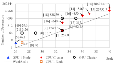
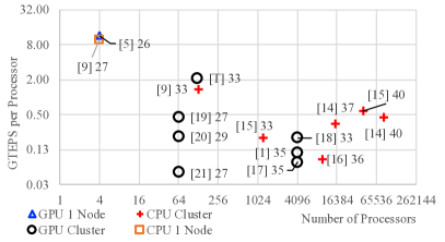
Figure 1: Placing our work (marked [T]) in the context of other large-scale BFS projects. GPU clusters are black circles and CPU clusters are red crosses. Two symbols mark top single-node CPU [9] and GPU [5] accomplishments. Left: RMAT scale (graph size) vs. number of processors to process a graph at that scale. Results nearer the bottom right can process larger graphs with fewer processors. The dashed line represents the weak scaling line corresponding to our scale-processor count. Annotations mark aggregate GTEPS. Right: Cluster size vs. throughput (edges processed per second) per processor. Results nearer the top right sustain higher throughput with more processors. Annotations mark maximum RMAT scale.

II-A Terminology

For ease of discussion, we define the following terms, and use them in later sections of the paper.

graph A graph $G(V,E)$ is defined by its vertices $V$ and edges $E$. In this paper, to study DOBFS scalability without doubling the storage size, we assume the graph is symmetric.

$\boldsymbol{n}$ $=|V|$, the number of vertices in the graph.

$\boldsymbol{m}$ $=|E|$, the number of edges in the graph.

$\boldsymbol{p_{\textit{rank}}}$ the number of Message Passing Interface (MPI) ranks.

$\boldsymbol{p_{\textit{gpu}}}$ the number of GPUs per MPI rank.

$\boldsymbol{p}$ $=p_{\textit{rank}}\cdot p_{\textit{gpu}}$, the number of GPUs used.

$\boldsymbol{g}$ the inverse of inter-node communication bandwidth.

$\boldsymbol{\mathit{TH}}$ the degree separation threshold (section III-A).

delegates vertices with out-degree larger than $\mathit{TH}$.

normal vertices vertices with out-degree at most $\mathit{TH}$.

$\boldsymbol{E_{nn},E_{nd},E_{dn},E_{dd}}$ normal $\rightarrow$ normal, normal $\rightarrow$ delegate, delegate $\rightarrow$ normal, and delegate $\rightarrow$ delegate edges.

$\boldsymbol{d}$ the number of delegates in the graph.

$\boldsymbol{S}$ the number of iterations (i.e., super-steps) of running BFS on the graph, bounded by the diameter of the graph.

II-B Challenges with Scaling Directional Optimization

Directional optimization is a widely adopted optimization used in high-performance BFS implementations. First described by Beamer, Asanović, and Patterson [4], it switches from the conventional forward-push (i.e. top-down) direction to the backward-pull (i.e. bottom-up) direction when the workload of visiting all neighbors of the newly discovered vertices from the previous iteration is greater than trying to find only one previously visited parent of the unvisited vertices. The workload savings from skipping a vertex’s parent list once a valid one is found can be huge, and it is very efficient for graphs with small diameters and dense cores, for example, social networks and RMAT graphs.

However, conventional DOBFS implementations face scaling issues in a cluster environment. When running in the backward-pull direction, each active (unvisited) vertex must know the status of all its possible parents. This information comes with a high communication cost. If the graph is 1D-partitioned, it forces broadcasting the newly visited vertices to all the peers that host their neighbors. In practice, this often results in broadcasting the newly visited vertices to every peer, which is $8m$ bytes in communication volume, and $8m/p\cdot g$ in communication time. If the graph is 2D-partitioned [10], it takes 2 hops to propagate the visiting status of vertices: one reduction across the row direction, and one broadcast across the column direction.

Let us use $n_{t}$ to indicate the number of vertices visited in the forward-push iterations, and $S_{b}$ to indicate the number of iterations in the backward-pull direction. We make the following assumptions: 1) row- and column-wise vertex numbers are 32-bit; 2) reduction and broadcast works in a tree-like manner, which gives $\log{\sqrt{p}}$ communication for each column or row; 3) the same vertex is never visited in more than one iteration, otherwise the communication cost will be higher; and 4) the processor grid is square, i.e., there are equal divisions in the row and the column directions. Then the total communication volume for the forward direction is $8n_{t}\sqrt{p}\log{\sqrt{p}}$ bytes, and it is $2nS_{b}\sqrt{p}(\log{\sqrt{p}})/8$ bytes for the backward direction using compressed bit masks. The communication time is $(4n_{t}+nS_{b}/8)((\log{\sqrt{p}})/\sqrt{p})\cdot g$. When the graph size and the number of nodes increase at the same rate (weak scaling), the above communication cost will increase as $\sqrt{p}$, and this limits the scalability on large systems. There are also increases in the computation workload: instead of finding only one valid parent for each unvisited vertex, the 2D partitioned case tries to finds $\sqrt{p}$ valid parents, one in each of the $\sqrt{p}$ row-partitions of an unvisited vertex. When running on large clusters, i.e. $\sqrt{p}$ is large, this workload increase defeats the workload saving purpose of DO. In summary, both 1D and 2D partitioning within a cluster on a DOBFS present significant scalability challenges.

Previous work on large-scale BFS falls into three categories. Single-node projects, either CPU or GPU, generally sustain the highest throughput per processor but are limited by storage or compute to relatively modest graph scales. The largest CPU clusters (tens of thousands of nodes) have addressed the largest graph scales ($\geq 36$), whereas smaller-sized GPU clusters (thousands of nodes) have not yet reached that scale. As a gross generalization, CPU implementations are limited in scalability by computation (they must add nodes to have more compute resources to process larger graphs), whereas the GPU ones are limited by memory size (they must add nodes to have more memory to store larger graphs). We summarize this work in figure 1.

II-C BFS within Single Node

Using GPUs in the same node for BFS yields impressive per-node performance [5, 9, 11, 12], but because all their communication is within a node and thus faster than within a cluster, their per-node performance is superior to cluster-based solutions. However, their graphs must fit into one node’s memory (GPU or CPU), and this inherently limits the maximum size of a processed graph.

To break this memory limitation, other researchers have used a shared memory architecture [9] or high-speed local storage [13]. The shared memory architecture is essentially multiple nodes with unified memory space, and it is less common than distributed memory architectures. Using fast local storage can help to process huge graphs with limited hardware resources, but moving large amounts of graph data limits overall traversal performance.

II-D BFS on CPU Clusters

The Graph500 list is mostly CPU cluster implementations [14, 15, 16], which use a large number of processors, typically more than 10k, to reach the reported performance.

These implementations tend to use very specific graph representations [2, 14], which may not be GPU-friendly, because their complex memory access patterns bring extra irregularity and more branching conditions, both of which reduce achievable parallelism on GPUs. We instead choose a standard graph representation (CSR). We expect our BFS implementation will be used as a component of a complex workflow with many components that use standard formats for passing data between them. Using non-standard graph representations requires such a workflow to incur an additional cost of format conversion, to duplicate graphs, or to redesign other components, none of which are desirable.

These implementations also generally use 2D partitioning to distribute the graph across processors. 2D partitioning may introduce a high communication cost (Section II-B). As subgraph sizes on each processor increase (to make full usage of more capable nodes as the number of nodes decreases), the data transmitted per node will increase together with the graph size, but the bisection network bandwidth will be lower as the network shrinks. Machine-specific network optimization could help, but this direction may make the implementation less applicable to other systems.

The recent implementation by Yasui and Fujisawa [9] shows a significant improvement in per-processor performance, using a shared memory system with 128 processors. In this work, the subgraph size on each processor is considerably larger than previous BFS work on CPU clusters. With upcoming supercomputers featuring a smaller number of nodes with more resources per node, using larger sub-graphs per processor may be more suitable for upcoming machines.

II-E BFS on GPU Clusters

BFS on GPU clusters is a relatively recent topic of study [17, 18, 1] (citation [1] here refers to TSUBAME 2.0’s number 31 ranking in the June 2017 Graph500 list. The achieved performance is 462.25 GTEPS with scale 35 using 4096 Tesla GPUs in 1366 nodes. We can’t find published work that references this particular record.), with some recent work focusing on a smaller number of GPUs [19, 20, 21]. None of this work demonstrates competitive per-node performance vs. single-node work, and none shows the combination of scalability and performance per node that we demonstrate in this work.

III Graph Representation

The key to a scalable DOBFS on a GPU cluster is to (a) maximize the fraction of the graph that can be stored on one GPU, thus allowing fast computation with no communication on that portion of the graph, and (b) optimize the communication between GPUs, which would otherwise limit scalability, even within a single node [5].

III-A Separation of Vertices

Our design to accomplish these goals starts from a simple but powerful idea that we have pursued in previous work on CPU clusters [8]: separate the vertices into two sets by out-degrees, and treat them differently. The separation point between the two, the threshold out-degree $\mathit{TH}$, is an important tuning parameter, and we will show how it affects the overall performance in upcoming sections. We call vertices with more than $\mathit{TH}$ direct neighbors the delegates, and the rest normal vertices.

The intuition behind this design choice is that in local traversal, vertices at different ends of the degree distribution should have different load-balancing strategies; and in communication, vertices that almost every GPU touches should not be treated the same as those needed by very few GPUs. By separating vertices into different sets, we can pursue different strategies in graph representation, local traversal, and communication on those sets, which we describe below.

III-B Distribution of Edges

  Algorithm 1 Edge Distributor

 

1:Let $P(v)=\bmod(v,p_{\mathit{rank}})$

2:Let $G(v)=\bmod(v/p_{\mathit{rank}},p_{\mathit{gpu}})$

3:for each edge $(u\rightarrow v)$ do:

4:     if $u$ is normal then: to rank $P(u)$, GPU $G(u)$

5:     else if $v$ is normal then: to rank $P(v)$, GPU $G(v)$

6:     else if $(\mathit{OutDegree}(u)<\mathit{OutDegree}(v))$ then:

7:         to rank $P(u)$, GPU $G(u)$

8:     else if $(\mathit{OutDegree}(u)>\mathit{OutDegree}(v))$ then:

9:         to rank $P(v)$, GPU $G(v)$

10:     else: to rank $P(\min(u,v))$, GPU $G(\min(u,v))$

11:     end if

12:end for

 

On scale-free graphs, most storage is devoted to edges, not vertices. We distribute edges to individual MPI ranks, and then to individual GPUs within the same rank, using the distributor described in Algorithm III-B. In it, we divide edges into four categories depending on the type of their source and destination vertices (normal or delegate). Our edge distributor has the following advantages:

Simple The location of an edge can be easily computed from its index locally without table lookup or remote query.

Symmetric Except for normal to normal edges, subgraphs on individual GPUs are symmetric. Because we make an edge pair of opposite directions for an undirected edge, they need to be on the same GPU to preserve the correctness of DOBFS without a global traversal direction. Otherwise if the traversal directions of the edge pair are opposite to their respective directions, both edges will be ignored.

Bounded size The number of possible destination vertices for non-(normal to normal) edges on each GPU are bounded: the number of normal vertices is at most $n/p$, and the number of delegates is at most $d$. Thus vertex indices for these edges can be represented as 32-bit numbers locally, and converted back to 64-bit when necessary for communication. This allows us to store more of the graph in a fixed-size memory.

Balanced This distribution prioritizes placement of vertices with lower out-degrees. Neighbor lists of high-degree vertices are distributed according to the destination vertices, and scattered across the entire cluster. The number of edges in the partitioned subgraphs on individual GPUs are very close to each other, giving each GPU a balanced workload.

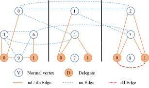
Figure 2: Example of degree separation and edge distribution for a graph with 3 partitions and degree threshold 5. Top: the original graph. Bottom: subgraphs after making vertex 7 as delegate 0, and vertex 8 as delegate 1. nd, dn, nn and dd refer to normal to delegate, delegate to normal, normal to normal, and delegate to delegate edges, respectively.

Figure 2 illustrates our vertex separation and edge distribution strategies. Vertices 7 and 8 have out-degree more than $\mathit{TH}$, which is 5 in this example, and they are converted to delegates 0 and 1, respectively. All partitions keep a copy of the delegates, and all edges involving the delegates are changed to the local copies. After this operation, only edges between normal vertices require communication across GPUs; all other edges are between two vertices on the same GPU. This is the right choice because normal vertices are the ones with the fewest neighbors and thus the least communication. Any delegate-related communication is performed using global reductions (details in section 4).

III-C Efficient Graph Storage

sub-graph	row offsets	column indices
nn	$n/p\cdot 4$	$|E_{\textit{nn}}|/p\cdot 8$
nd	$n/p\cdot 4$	$|E_{\textit{nd}}|/p\cdot 4$
dn	$d\cdot 4$	$|E_{\textit{dn}}|/p\cdot 4$
dd	$d\cdot 4$	$|E_{\textit{dd}}|/p\cdot 4$
Total	$8n+8d\cdot p$	$4m+4|E_{\textit{nn}}|$

TABLE I: Memory usage for subgraphs in bytes.

The bounded-size feature of our edge distributor is critical for processing huge graphs within limited GPU device memory, and makes processing larger graphs using the same number of GPUs possible. When the number of local normal vertices and the number of delegates are bounded by $n/p$, with the exception of destinations of nn edges, we can use 32-bit values to store local normal vertex and global delegate ids, instead of 64-bit values. This provides significant savings on the memory storage footprint of the graph. As listed in Table I, the total memory usage for all subgraphs on the GPUs is $8n+8d\cdot p+4m+4|E_{\textit{nn}}|$ bytes. In practice, when using suitable values of $\mathit{TH}$ (Section VI-B), while still using CSR format for each sub-graphs, the above memory usage is only about one third of the conventional edge list format ($16m$ bytes), and a little more than half of CSR format ($8n+8m$) without the degree separation.

It is possible to utilize CPU memory and handle graphs larger than GPU memory, with different techniques [22, 23]. However, the current latency and bandwidth differences between GPU memory and the GPU-CPU connection would impose a high performance penalty. This decision could be revisited when CORAL is fully equipped with NVLink2, which doubles CPU-GPU bandwidth, in the near future. In this paper, we only focus on graphs that fit in GPU memory.

IV Local Computation

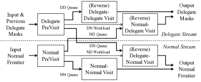
Figure 3: Local computation for one BFS iteration, showing data dependency and stream allocation.

On each GPU, we now have 4 different subgraphs: normal to normal (nn), normal to delegate (nd), delegate to normal (dn) and delegate to delegate (dd). While we could apply the exact same strategies to each of them, we note that their different characteristics motivate different load-balancing strategies for traversal (Section IV-A), different direction switching conditions for DOBFS (Section IV-B), and different input from/output to the communication model (Section V). Because subgraphs can be processed in parallel, we can achieve some overlap between computation and communication in our processing pipeline (Fig. 3).

At a high level, we separate local traversal on the four subgraphs into a delegate stream and a normal stream, depending on the destination type of the edge, as two cudaStreams. Each stream begins with a “previsit” kernel, used to preprocess the inputs. This includes marking level labels for input vertices, filtering out duplicates and zero-out-degree vertices, forming the queues of vertices to be visited by the visit kernels, and calculating the would-be workload for these kernels, which is important for the direction decisions in DO. Then each stream spawns a “visit” kernel for the two edge types in the stream. The two streams run independently of each other, except when dependencies are established explicitly (Fig. 3).

IV-A Forward Traversal

The visited status of delegates are maintained by bitmasks, with each delegate only occupying 1 bit. This is an effective way to store and communicate the status of high out-degree vertices. We use advanced load balancing techniques for the visiting kernels: the delegate to delegate visit kernel uses merge-based workload partitioning [24], because the dd subgraph covers a wide range of degree distribution, and has large average out-degrees; the other visit kernels use thread-warp-block dynamic workload mapping [25], based on the fact that the out-degree range of dn, nd, and nn subgraphs are all limited, and the average out-degrees are low.

IV-B Directional Optimization

Not all subgraphs benefit from directional optimization. We do not use DO for normal $\rightarrow$ normal visits, because the nn subgraph on each GPU is not symmetric, the range of destination vertices of nn edges are unbounded, and most importantly, DO is not efficient for the very low in-degree nn subgraphs. Without separating the graph, skipping the nn portion from using DO is impossible.

On each GPU, we keep a source list of the normal-to-delegate subgraph, i.e., all the normal vertices that have edges pointing to delegates. These are exactly the potential destination vertices in the reverse subgraph, i.e., the delegate to normal subgraph. When running in the backward-pull direction for a delegate to normal visit, we use the normal-to-delegate subgraph, and start from its source list. For the same purpose, we keep source masks for the dd and dn subgraphs. Keeping source lists and masks avoids vertices that may not find local parents, and provides more accurate workload prediction.

The traversal direction is decided based on a workload comparison, computed in each iteration, between the forward and the backward directions. The forward workload $\mathit{FV}$ is calculated by the previsit kernels as the sum of neighbor list lengths from the source vertices to be visited. The backward workload $\mathit{BV}$ is calculated using the estimated number of parents to check until finding the first visited one. Let:

$$U =\text{unvisited sources in the reversed graph};$$

$$q =\text{input frontier length};$$

$$s =\text{number of unvisited sources in the forward graph};$$

$$a =\text{probability that a potential parent is newly visited};$$

$$=q/(q+s);$$

$$od(u) =\text{out degree of u};$$

$$\text{Then: }BV =\sum_{u\in U}((1-a)^{od(u)}+\sum_{i=0}^{od(u)-1}a(1-a)^{i})$$

$$=\sum_{u\in U}\frac{1-(1-a)^{od(u)}}{a}\approx|U|/a$$

$$\text{assuming }od(u)\text{ is large, \& }a\text{ not too small}$$

$$=|U|(q+s)/q$$

Starting from the forward-push direction, with two direction-switching factors $\mathit{factor0}$ and $\mathit{factor1}$, the visiting direction is decided as:
if current direction is forward, and $\mathit{FV}>\mathit{factor0}\cdot\mathit{BV}$
      then switch to backward;
if current direction is backward, and $\mathit{FV}<\mathit{factor1}\cdot\mathit{BV}$
      then switch to forward;
otherwise keep current direction.

No matter which direction a visiting kernel takes, it only affects the kernel itself, and the input and the output are the same. The three visiting kernels with DO have three sets of direction-switching factors. This allows the kernels to switch for their own optimized conditions.

Our strategy for DOBFS results in a smaller workload than a 2D partitioning strategy. In our strategy, for normal vertices, only one GPU must do the reverse visiting for each individual normal vertices. Only the delegates may need to have more than one GPUs visiting their parents, and moreover, the delegates are only a small portion of all vertices. Let $m^{\prime}$ be the number of edges the DOBFS algorithm would need to visit if the graph was traversed by a single processor. Then the workload of our DOBFS implementation would be bounded by $m^{\prime}+dp\cdot b$, where $b$ is the average number of parents a delegate must search on each GPU before finding a visited one. While keeping $d$ in the order of $O(n/p)$, the term $dp\cdot b$ is scalable even when $p$ is large, because it is in the order of $O(nb)$ and $b$ is not a large number—only delegates with very large out-degrees are distributed across a large number of nodes, and delegates with large out-degrees tend to be close to portions of the graph with high connectivity, which reduces the number of neighbors to try before finding a visited one.

V Communication

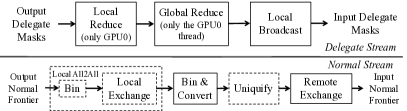
Figure 4: Communication flow

Because local computation performance is increasing more quickly than interconnect bandwidth, designing for scalable communication is more important for graph processing than ever before. Our scalable communication model (shown in Fig. 4) adopts different strategies for delegates and normal vertices.

V-A Communication for Delegates

The visited status of delegates may be updated by any GPU, or consumed by any GPU. We thus use a global reduction to gather and distribute the delegate mask updates whenever any update occurs in a iteration. The reduction is done in two phases: locally across peer GPUs, and globally across different MPI ranks. During the local phase, all GPUs in the same MPI rank push their updated masks to GPU₀, and GPU₀ performs the reduction in parallel. During the global phase, only GPU₀ (more accurately, the CPU thread that controls GPU₀) participates, and all GPUs in the same MPI rank consume the resulted masks for the next iteration. We utilize fast GPU-GPU data channels and the GPU’s parallel computing capability for the local phase, and efficient MPI_(I)AllReduce calls for the global phase.

The cost of this delegate communication is small. For each iteration that has updates to the delegate masks, the communication volume is $2dp_{\textit{ranks}}/8$ bytes, and the communication time is $d\log{p_{\textit{ranks}}}/4\cdot g$, assuming the global reduction is done in a tree-like manner. The delegate reduction might run on every iteration, which gives the total communication cost as $d\log{p_{\textit{rank}}}/4\cdot gS$. However, for graphs with more concentrated cores, the delegate updates will finish faster than normal vertices, which reduces the number of iterations that require delegate communication. In practice, we keep $d$ (the number of delegates) low, so that the size of delegate masks, $d/8$, is under the limit of several tens of MBs.

V-B Communication for Normal Vertices

The basic communication model for normal vertices is point-to-point transmission via MPI_Isend and MPI_Irecv. We use a non-blocking version to keep the pipeline running and take advantage of possible workload overlaps. The total communication volume is $4|E_{\textit{nn}}|$ bytes, assuming each nn edge is a cutting edge (i.e., a edge with end points on two different GPUs). The communication time is $4|E_{\textit{nn}}|/p\cdot g$. Note that only the outputs from nn edge visits may result in direct remote normal vertex updates: the results from dd and nd edge visits are communicated via global delegate mask reduction, and the updates from dn visits are always local, as a result of our edge distributor (Algorithm III-B). When setting $\mathit{TH}$, the degree threshold, to an optimal value, the nn edges are only a small portion of the graph, and the resulting normal communication is a lot less than $m$.

The normal vertex exchange requires some extra local computation, such as binning (group vertices need to be sent to the same GPU together) and vertex number conversion (from the 64-bit global ids used in nn edge destinations to 32-bit local ids at destination GPUs). These computations are done on GPUs. The workload is in the order of $O(|E_{\textit{nn}}|/p)$ on each GPU for all iterations combined. This is a small cost compared to the traversal workload, and does not affect the scalability of our BFS implementation.

We also tried two optimizations to reduce communication cost. The first one is called Local All2all: prior to the remote vertex exchange, we first run a local exchange to gather vertices going to GPU_xs in all MPI ranks on the local GPU_x. As a result, normal vertex exchanges only occur among GPU₀s, among GPU₁s, etc., but never between GPU₀s and GPU₁s, etc. This reduces the number of communication pairs from $p^{2}$ to $p^{2}/p_{\textit{gpu}}$, each of which has more vertices to send. In turn, this allows a second optimization, uniquification, which removes duplicated vertices going to the same GPU. However, because relatively few individual destination vertices of nn edges are on a given GPU or node, with the expected value capped by $\mathit{TH}/p_{\textit{rank}}$, the chance to find duplications is small, and may not be sufficient to overcome the extra computation. We show our findings in the next section.

Combining the communication for delegates and normal vertices together, we have a model that has at most $dp_{\textit{ranks}}/4\cdot S+4|E_{\textit{nn}}|$ bytes total volume and $(d\log{p_{\textit{ranks}}}/4\cdot S+4|E_{\textit{nn}}|/p)g$ communication cost. For graphs that have a small number of vertices covering a large portion of edges, the number of iterations $S^{\prime}$ that need delegate masks exchange, is less than $S$; for the graphs we tested, $S^{\prime}$ is about half of $S$. With suitable values of $\mathit{TH}$ (Section VI-B), we saw delegate mask reduction and normal vertex exchange taking roughly the same amount of time. Under these conditions, we approximate our communication cost as $d\log{p_{\textit{rank}}}/4\cdot Sg$. We also keep $d$ on the same scale as $n/p$, more accurately, under the value of $4n/p$ in practice. As a result, the communication cost is $n\log{p_{\textit{rank}}}/p\cdot Sg$. It starts from $n\cdot Sg$ on single node, and grows on the order of $\log{p_{\textit{rank}}}$ when $n$ and $m$ increase at the same rate as $p$ (weak scaling). This growth is slow, and more scalable than the $\sqrt{p}$ growth order of conventional 2D partitioning methods. Thus, we argue that our communication model is more scalable.

VI Results

VI-A Testing Environment

VI-A1 Hardware

Our implementation targets an early access system (Ray) of LLNL’s upcoming CORAL/Sierra supercomputer. The current system has more than 40 compute nodes; each features two 10-core IBM Power8+ CPUs at 2.06 GHz with 256 GB CPU memory. Each CPU has two NVIDIA Tesla P100 GPUs; the two GPUs and the CPU are connected by high-speed NVLink [26] with 40 GB/s bandwidth in each direction. Each socket has a Enhanced Data Rate (EDR) 100 Gbps InfiniBand connection to a network with FatTree topology.

Because the interconnection speed is higher than a conventional cluster, and because GPUs achieve their best performance only when fully occupied by a sufficient workload, we first test how the network performs with different message sizes. In an experiment, we use 32 nodes, each with one MPI rank, and 4 CPU threads, and each thread sending MB-sized data to all threads on other nodes, to simulate a scenario where each of the 128 GPUs sends out data to the 124 GPUs on other nodes. After sweeping through the message size from 128 kB to 16 MB, we found that the optimal message size is about 4 MB for data larger than 2 MB. While this is much larger than normal MPI usage, it is the best fit for the GPUs. With smaller data (under 2 MB), the network appears to do a better job with caching, and the differences between message sizes are not that significant.

VI-A2 Software

The cluster runs on 64-bit Linux with GPU driver version 384.59. The compilation toolchain includes gcc 4.9.3, cuda 9.0.167, and spectrum-mpi 2017.08.24 with OpenMP support. nvcc options are -O3 –std=c++11 –expt-extended-lambda. The GPU target is set to the hardware’s SM version (i.e., 6.0 for P100 GPUs).

At the time of our experiments, we faced the following current limitations with Ray. Many of these will be addressed in the full system or with system software updates.

• Network Interface Controller (NIC)-GPU Remote Direct Memory Access (RDMA) was not planned for Ray; instead all NIC-GPU traffic goes through CPU memory.

• Asynchronous GPU memory copy was not supported by the MPI implementation; as a workaround, our implementation copies data from GPU memory to CPU memory with appropriate cudaMemcpyAsync calls, then issues MPI calls from the CPU memory, and copies the data from CPU to GPU on the receiving end.

• Random delays of $\sim$100 ms were observed when consuming data on CPU right after receiving them from unblocking MPI calls; as a result, we only use the CPUs for GPU workload scheduling and data movement controls in our experiments.

• Degraded data movement performance between CPUs and GPUs were observed on some nodes; all but one experiments only use up to 124 GPUs on 31 selected nodes to avoid this issue; the experiment with the WDC 2012 graph includes 3 GPUs affected by this issue, out of 160 GPUs on 40 nodes.

VI-A3 Reporting

We use RMAT graphs for testing our BFS implementation. The RMAT graph generator is a distributed GPU implementation conforming to the Graph500 specifications [1]. The edge factor is 16, and the RMAT parameters are ${A,B,C,D}={0.57,0.19,0.19,0.05}$. For a given RMAT graph at scale $N$, the number of vertices $n$ is $2^{N}$; the number of edges $m$, after making the graph undirected by edge doubling, is $2^{N}\cdot 32$. However, following the Graph500 specification [1], we only use $m/2=2^{N}\cdot 16$ to calculate the edge traversal rate. Vertex numbers are randomized using a deterministic hashing function after edge generation.

Our implementation outputs the hop-distances from the source vertex, instead of the BFS tree required by Graph500. The cost of building such a tree should be low in our implementation: only the destination vertices of nn edges, without possible delegate parents, would need to communicate their parent information at the end of BFS; vertices visited by dd, dn, and nd kernels can get the parent information locally, with almost no extra cost to the local computation.

For each reported data point, we executed 140 BFS runs with randomly generated sources; only the ones that executed for more than 1 iteration are considered. We report the geometric mean of edge traversal rates (in the unit of Giga Traversal Edges Per Second, GTEPS) or elapsed times (in the unit of milliseconds, ms).

We use number of nodes $\times$ number of MPI ranks per node $\times$ number of GPUs per MPI rank to denote the hardware for our experiments and for prior work. For example, $4\times 1\times 2$ means 4 nodes with 1 MPI rank per node, and 2 GPUs per MPI rank, 8 GPUs in total.

VI-B Parameter Settings

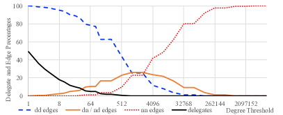
Figure 5: Distribution of different kinds of edges and delegates, as a function of degree threshold, for a scale-30 RMAT graph.

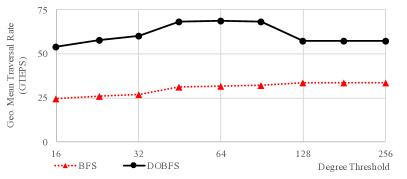
Figure 6: Traversal rates vs. degree threshold, for a scale-30 RMAT graph with $4\times 1\times 4$ GPUs.

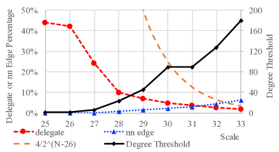
Figure 7: Suggested degree thresholds for different RMAT scales, with the resulting delegate and nn edges percentages. The $4/2^{N-26}$ line is the percentage of $4n/p$ vertices when using scale 26 RMAT graph per GPU.

Our implementation has several parameters and options that can be used to tune performance. The single most important parameter is the degree threshold $\mathit{TH}$. By changing $\mathit{TH}$, we are balancing the percentages of delegates and nn edges. Generally we want $d$ to be on the same order as the number of local vertices $n/p$; in our experiment, we keep $d$ under $4n/p$. It would also be desirable to keep the nn edge percentage under 10%. Figure 5 shows how $\mathit{TH}$ changes the distributions of vertices and edges on the scale-30 RMAT graph. Any $\mathit{TH}$ in the range of $[16,512]$ will satisfy our goal. We sweep this range to see the resulted performance, as shown in Figure 6. The actual range that gives the best performance for both BFS and DOBFS is quite wide, from 45 to 90; we use 64 in our experiments.

With a similar experiment, we suggest degree thresholds for a wide range of graph scales (Fig. 7). The optimal $\mathit{TH}$ increases at the rate of about $\sqrt{2}$ per scale. For scales up to 33, the delegate percentage is well below the $4n/p$ line; at scale 33, the delegate percentage is 1.75%, and the $4n/p$ line is at 3.23%. The nn edge percentages increases slightly, to 6.3% at scale 33, which is still a small and acceptable percentage. For larger scales that may lead to insufficient GPU memory caused by a large number of delegates or nn edges, the following options may be considered: 1) increase $\mathit{TH}$ to decrease the number of delegates, as a range of values yield similar performance; 2) increase $p$ to reduce the memory usage per GPU, as there is no limitation on how many GPUs can be used, provided that the GPU memory is sufficient. With these two options, we believe our method could continue to scale on larger GPU clusters.

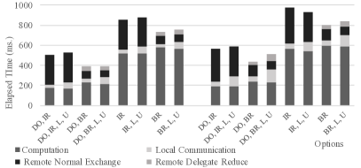
Figure 8: Effect of different options on performance. DO stands for directional optimization; L for local-all2all; U for uniquify; IR for unblocking delegate mask reduction; and BR for blocking reduction. The graph is RMAT scale 32 with degree threshold 128, with a $16\times 2\times 2$ hardware configuration on the left and $16\times 1\times 4$ on the right.

We can tune our implementation with several options: directional optimization (DO), local all2all (L), uniquify (U), blocking global mask reduction (BR) using MPI_Allreduce or unblocking reduction (IR) using MPI_Iallreduce, and hardware configuration (e.g., a $*\times 2\times 2$ or $*\times 1\times 4$ setup). Figure 8 shows how different options affect the timings of different parts of the BFS runtime. DO cuts the computation time by a factor of three, even when the workload is distributed on 64 GPUs. L and U add a small amount of time to local data exchange, but do not have a significant impact on the global communication time, mainly because the degree threshold $\mathit{TH}$ is so low that we see few duplications in the normal vertex exchange. BR significantly reduces the communication time in this example, although the actual volumes of communication are the same. This may be a consequence of an unoptimized implementation of MPI_Iallreduce, a newly available feature on this machine. When running on fewer than 8 nodes, the communication time of IR is less than that of BR. We hope the same applies to a larger number of nodes so that the advantage of workload overlapping can be fully explored. The sum of all parts in one column is more than the elapsed time of BFS, because different parts may overlap. For example, visiting from the delegates can start once the delegate masks are received without waiting for the normal vertices. For this particular experiment, the overlaps reduce the running time by about 10% on average when compared to the sum of all parts.

For each of the three subgraphs that apply DO, our implementation has two direction-switching factors that decide when to change the traversal direction. For RMAT, once the traversal switches to the backward direction, it does not need to change back; as a result, we only have three factors to decide. After scanning these factors from $10^{-8}$ to $10$ for the best performance, we found out that all three factors have a wide range of near-optimal values; in fact, the same range ($0.5,0.05,1\times 10^{-7}$) for dd, dn, and nd subgraphs applies to almost all configurations that follow the weak scaling curve and the suggested $\mathit{TH}$ values. From our experience, these selections are similar for the same type of graphs.

VI-C Overall Results and Comparisons

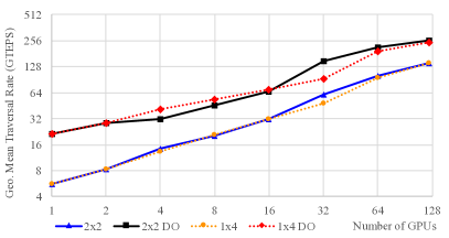
Figure 9: Weak scaling with a scale-26 RMAT graph per GPU

Figure 9 shows overall weak scaling curves, with $\sim$scale-26 RMAT graphs on each GPU up to 124 GPUs. In this range it is mostly linear, peaking at 259.8 GTEPS for RMAT scale 33 on 124 GPUs. From 16 GPUs to 32 GPUs, we switch from MPI_Iallreduce to MPI_Allreduce, as discussed earlier in this section, which introduces performance increases higher than the average.

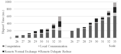
Figure 10: Runtime breakdown for $*\times 2\times 2$ setup along the weak scaling curve. DOBFS is on the left, and BFS on the right; scales 28 to 30 use unblocking global delegate mask reductions and merge communication time for masks and normal vertices; scale 31 to 33 use blocking global delegate mask reduction. Because of overlap, the sum of different parts in a column is not equal to the BFS running time.

Figure 10 shows detailed timing for DOBFS and BFS at different scales. Local visiting time grows slowly, only $4\times$ over 7 scales for DOBFS as the graph size and the number of GPUs increase to $124\times$. The BFS computation time increases to $3\times$ for the same range. This shows the computation is scaling as expected. The communication grows slightly faster than the computation, especially from scale 32 to 33. This may be caused by the increases in number of delegates and nn edges, as shown previously in Figure 5 and Section VI-B, or it may be traffic conditions in the network, as about 70% of the nodes in the cluster are actively transmitting large amounts of data. Because our implementation overlaps communication and computation, we mitigate the effects of this increase in communication cost. Both computation and communication appear to successfully scale throughout this range of RMAT sizes.

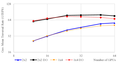
Figure 11: Strong scaling with a scale-30 RMAT graph.

Figure 11 shows strong scaling curves using the scale-30 RMAT graph. Because of our efficient graph representation, we can fit the 34 billion edge graph onto 12 GPUs, at about 2.9 billion edges per GPU. The performance of DOBFS increases 29% when using 24 GPUs instead of 12, and the strong scaling curve stays almost flat after 24 GPUs. When using more GPUs, the timing improvement in computation is about the same as the increase in communication, caused by delegate masks reduction across more nodes and more cutting nn edges. On more than 48 GPUs, the communication time is dominant and the GPUs are under-utilized, thus the performance starts to drop. BFS yields better strong scalings than DOBFS, primarily because of its comparably larger computation workload.

scale	ref.	ref. hw.	ref. comm.	ref. perf.	our hw.	our perf.
{24, 25, 26}	Pan [5]	1$\times$1$\times${1, 2, 4} Tesla P100	single node	{31.6, 42.9, 46.1}	1$\times$1$\times${1, 2, 4} Tesla P100	{22.9, 32.5, 39.8}
33	Bernaschi [18]	4096$\times$1$\times$1 Tesla K20X	Dragonfly 100Gbps	828.39	31$\times$2$\times$2 Tesla P100	259.8
29	Krajecki [20]	64$\times$1$\times$1 Tesla K20Xm	FatTree 10Gbps	13.7	2$\times$1$\times$4 Tesla P100	53.13
33	Yasui [9]	128$\times$10$\times$1/10 Xeon E5-4650 v2	shared memory	174.7	31$\times$2$\times$2 Tesla P100	259.8
33	Buluc [16]	1204$\times$1$\times$1 Xeon E5-2695 v2	Dragonfly 64Gbps	$\sim$240	31$\times$2$\times$2 Tesla P100	259.8

TABLE II: Comparison with previous works.

We compare our results with previous efforts in Table II. When compared against single-node multi-GPU Gunrock [5], this work is a little slower when using the same graphs, which may be the effect of more optimizations in Gunrock’s traversal kernels. As we add more GPUs in this work, we see the gap in performance is narrowing, which indicates better scalability; and the memory size improvements we made in this paper allows us to process larger graphs on one node, up to scale 28 on 4 GPUs, than any other GPU-based previous work.

Compared to Bernaschi et al. [18], our work achieves about 31% of their performance with only 3% the number of GPUs. Although the GPUs they used are not as new as ours, the 10$\times$ per-GPU performance shows our efficient computation and communication. Compared to Krajecki, Loiseau, Alin, and Jaillet [20], we achieve 4$\times$ the performance using only one eighth the number of GPUs.

The flagship shared-memory CPU implementation by Yasui and Katsuki [9] uses a similar number of processors; we obtained 1.49$\times$ the performance of their work, which we believe is partially because of the performance advantages of the GPU. We also demonstrate slightly better performance than Buluç et al. [16] despite their 8.4$\times$ more processors.

VI-D General Graphs and Applications

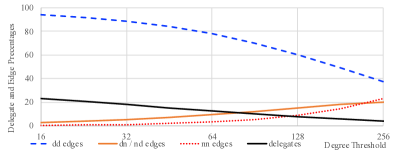
Figure 12: Distribution of different kinds of edges and delegates, as a function of degree threshold, for the friendster graph.

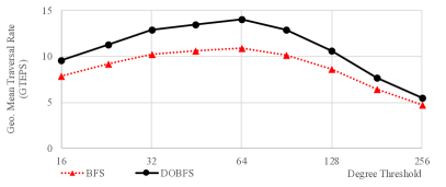
Figure 13: Traversal rates vs. degree threshold, for the friendster graph with $1\times 2\times 2$ GPUs.

We are also interested in graphs more general than RMAT, and use the Friendster graph [27] to test our implementation. We prepare this graph by randomizing the vertex numbers and make the graph symmetric by edge doubling. The resulting graph has 134 million vertices, about half of which are isolated ones, and 5.17 billion edges. Figure 12 shows how the distribution of different kinds of edges and vertices change with regard to various degree thresholds $\mathit{TH}$, and Fig. 13 shows the resulting performance. Similar to RMAT, the friendster social network has a wide range of suitable $\mathit{TH}$ values, in $[16,128]$. There is also a wide range $[32,91]$ of $\mathit{TH}$ values that gives close to the best performance.

We also analyze the Web Data Common (WDC) 2012 hyperlink graph [28], but reduce the hyper edges into single ones. Vertex-randomization and edge-doubling give a graph with 4.29 billion vertices, 402 million of which are zero-degree ones, and 224 billion edges. Using 160 GPUs in a $40\times 2\times 2$ setup, our implementation achieves 84.2 GTEPS and 79.7 GTEPS, for BFS and DOBFS respectively, both using degree threshold 256. The BFS searches have about 330 iterations at average, and experience long-tail behavior. The averaged per-iteration time of 8 $\mu$S is not much more than the per-iteration overhead of a few $\mu$S. In this situation, the additional workload for direction decisions in DOBFS is more than the workload saving in traversal. As a result, the DOBFS performance is slightly less than BFS.

For algorithms more general than BFS, in most cases, the local computation is at least in the order of $O(m)$, much larger than that of DOBFS. They also introduce larger communication volumes: BFS only needs 1 bit for the visited status of delegates, and 32 bits for newly visited normal vertices of cutting nn edges across GPUs. Other graph algorithms require more bits of state for delegates—for example, ranking scores for PageRank—and associative values for normal vertices in additional to the vertex numbers themselves. For large scale-free graphs, the increases in computation and communication are roughly in the same order, and our computation and communication models should still be scalable. For graph processing that yields insufficient local workloads over many iterations, either caused by the graph topologies or the algorithms, we argue that they may not be suitable for Bulk Synchronous Parallel (BSP) frameworks on systems with fat nodes: the GPUs will be underutilized, and the per-iteration overhead may well make such implementations unscalable. Asynchronous graph frameworks, such as HavoqGT [29] and Groute [12], may be more suitable for such workloads.

VII Conclusions

Base on the idea of separating vertices by out-degrees, we implemented a scalable BFS, consisting of an efficient graph representation, scalable and fast local computation kernels, and a scalable communication model. With 124 P100 GPUs on the CORAL EA system, we achieved 259.8 GTEPS on the scale 33 RMAT graph. The close-to-linear weak scaling indicates that our work successfully targets modern GPU clusters, which feature fewer nodes and more local computing power than previous systems.

We believe our work provides a better alternative to conventional 2D partitioning methods for scaling DOBFS, and is better aligned with the latest trend of supercomputers and large systems. Further exploration using even more GPUs in the range of thousands, when they are available, could bring us more insight into and solutions for the scalability problem.

Future work includes investigating graph applications beyond BFS. These applications need more local computation than just neighborhood queries, more communication than just 1-bit visited status, and more attributes on vertices and edges than a single label. While most techniques and optimizations for BFS should still be applicable, we hope to see further work in the components of graph representation, local computation, and remote communication, under more complex application scenarios.

References

- [1] “The June 2017 Graph500 list,” https://graph500.org/?page_id=254, Jun. 2017.
- [2] A. Buluç and J. R. Gilbert, “On the representation and multiplication of hypersparse matrices,” in Proceedings of the 22nd IEEE International Symposium on Parallel and Distributed Processing Symposium, ser. IPDPS 2008, Apr. 2008, pp. 1–11.
- [3] V. Agarwal, F. Petrini, D. Pasetto, and D. A. Bader, “Scalable graph exploration on multicore processors,” in Proceedings of the International Conference for High Performance Computing, Networking, Storage and Analysis, ser. SC ’10, Nov. 2010, pp. 46:1–46:11.
- [4] S. Beamer, K. Asanović, and D. Patterson, “Direction-optimizing breadth-first search,” in Proceedings of the International Conference on High Performance Computing, Networking, Storage and Analysis, ser. SC ’12, Nov. 2012, pp. 12:1–12:10.
- [5] Y. Pan, Y. Wang, Y. Wu, C. Yang, and J. D. Owens, “Multi-GPU graph analytics,” in Proceedings of the 31st IEEE International Parallel and Distributed Processing Symposium, ser. IPDPS 2017, May/Jun. 2017, pp. 479–490.
- [6] “Coral info,” Oct. 2017, https://asc.llnl.gov/coral-info.
- [7] “Ray - Livermore Computing,” Oct. 2017, https://hpc.llnl.gov/hardware/platforms/Ray.
- [8] R. Pearce, M. Gokhale, and N. M. Amato, “Faster parallel traversal of scale free graphs at extreme scale with vertex delegates,” in Proceedings of the International Conference for High Performance Computing, Networking, Storage and Analysis, ser. SC ’14, Nov. 2014, pp. 549–559.
- [9] Y. Yasui and K. Fujisawa, “Fast, scalable, and energy-efficient parallel breadth-first search,” in The Role and Importance of Mathematics in Innovation: Proceedings of the Forum “Math-for-Industry” 2015. Springer Singapore, 2017, pp. 61–75.
- [10] B. Vastenhouw and R. H. Bisseling, “A two-dimensional data distribution method for parallel sparse matrix-vector multiplication,” SIAM Review, vol. 47, no. 1, pp. 67–95, 2005.
- [11] H. Liu and H. H. Huang, “Enterprise: Breadth-first graph traversal on GPUs,” in Proceedings of the International Conference for High Performance Computing, Networking, Storage and Analysis, ser. SC ’15, Nov. 2015, pp. 68:1–68:12.
- [12] T. Ben-Nun, M. Sutton, S. Pai, and K. Pingali, “Groute: An asynchronous multi-GPU programming model for irregular computations,” in Proceedings of the 22nd ACM SIGPLAN Symposium on Principles and Practice of Parallel Programming, ser. PPoPP ’17, Feb. 2017, pp. 235–248.
- [13] S. Maass, C. Min, S. Kashyap, W. Kang, M. Kumar, and T. Kim, “Mosaic: Processing a trillion-edge graph on a single machine,” in Proceedings of the 12th European Conference on Computer Systems, ser. EuroSys 2017, Apr. 2017, pp. 527–543.
- [14] K. Ueno, T. Suzumura, N. Maruyama, K. Fujisawa, and S. Matsuoka, “Extreme scale breadth-first search on supercomputers,” in Proceedings of the 2016 IEEE International Conference on Big Data, ser. BigData 2016, Dec. 2016, pp. 1040–1047.
- [15] H. Lin, X. Tang, B. Yu, Y. Zhuo, W. Chen, J. Zhai, W. Yin, and W. Zheng, “Scalable graph traversal on Sunway TaihuLight with ten million cores,” in Proceedings of the 31st IEEE International Parallel and Distributed Processing Symposium, ser. IPDPS 2017, May/Jun. 2017, pp. 635–645.
- [16] A. Buluç, S. Beamer, K. Madduri, K. Asanovic, and D. A. Patterson, “Distributed-memory breadth-first search on massive graphs,” CoRR, vol. abs/1705.04590, 2017.
- [17] K. Ueno and T. Suzumura, “Parallel distributed breadth first search on GPU,” in Proceedings of the 20th International Conference on High Performance Computing, ser. HiPC 2013, Dec. 2013, pp. 314–323.
- [18] M. Bernaschi, G. Carbone, E. Mastrostefano, M. Bisson, and M. Fatica, “Enhanced GPU-based distributed breadth first search,” in Proceedings of the 12th ACM International Conference on Computing Frontiers, ser. CF ’15, May 2015, pp. 10:1–10:8.
- [19] Z. Fu, H. K. Dasari, B. Bebee, M. Berzins, and B. Thompson, “Parallel breadth first search on GPU clusters,” in Proceedings of the 2014 IEEE International Conference on Big Data, ser. BigData 2014, Oct. 2014, pp. 110–118.
- [20] M. Krajecki, J. Loiseau, F. Alin, and C. Jaillet, “BFS traversal on multi-GPU cluster,” in Proceedings of the 2016 IEEE International Conference on Computational Science and Engineering, ser. CSE 2016, Jul. 2016, pp. 594–599.
- [21] J. Young, J. Romera, M. Hauck, and H. Fröning, “Optimizing communication for a 2D-partitioned scalable BFS,” in Proceedings of the 2016 IEEE High Performance Extreme Computing Conference, ser. HPEC 2016, Sep. 2016, pp. 1–7.
- [22] O. Green and D. A. Bader, “cuSTINGER: Supporting dynamic graph algorithms for GPUs,” in Proceedings of 2016 IEEE High Performance Extreme Computing Conference, ser. HPEC 2016, Sep. 2016, pp. 1–6.
- [23] N. Sakharnykh, “Beyond GPU memory limits with unified memory on Pascal,” Dec. 2016, https://devblogs.nvidia.com/parallelforall/beyond-gpu-memory-limits-unified-memory-pascal/.
- [24] A. Davidson, S. Baxter, M. Garland, and J. D. Owens, “Work-efficient parallel GPU methods for single source shortest paths,” in Proceedings of the 28th IEEE International Parallel and Distributed Processing Symposium, ser. IPDPS 2014, May 2014, pp. 349–359.
- [25] D. Merrill, M. Garland, and A. Grimshaw, “Scalable GPU graph traversal,” in Proceedings of the 17th ACM SIGPLAN Symposium on Principles and Practice of Parallel Programming, ser. PPoPP ’12, Feb. 2012, pp. 117–128.
- [26] NVIDIA Corporation, “NVIDIA NVLink high-speed interconnect: Application performance,” NVIDIA Corporation, Tech. Rep., Nov. 2014, http://info.nvidianews.com/rs/nvidia/images/NVIDIA%20NVLink%20High-Speed%20Interconnect%20Application%20Performance%20Brief.pdf.
- [27] “Friendster social network dataset: Friends,” Jul. 2011, https://archive.org/details/friendster-dataset-201107.
- [28] “Web data commons - hyperlink graphs,” 2012, http://webdatacommons.org/hyperlinkgraph/.
- [29] R. Pearce, “HavoqGT,” 2015, https://github.com/LLNL/havoqgt.