A walk outside spheres for the fractional Laplacian: fields and first eigenvalue
Abstract
The solution of the exterior-value problem for the fractional Laplacian can be computed by a walk-outside-spheres algorithm. This involves sampling -stable Levy processes on their exit from maximally inscribed balls and sampling their occupation distribution. Kyprianou, Osojnik, and Shardlow (2017) developed this algorithm, providing a complexity analysis and an implementation, for approximating the solution at a single point in the domain. This paper shows how to efficiently sample the whole field by generating an approximation in , for a domain . The method takes advantage of a hierarchy of triangular meshes and uses the multilevel Monte Carlo method for Hilbert space-valued quantities of interest. We derive complexity bounds in terms of the fractional parameter and demonstrate that the method gives accurate results for two problems with exact solutions. Finally, we show how to couple the method with the variable-accuracy Arnoldi iteration to compute the smallest eigenvalue of the fractional Laplacian. A criteria is derived for the variable accuracy and a comparison is given with analytical results of Dyda (2012).
AMS subject classification: 65C05, 34A08, 60J75, 34B09.
Keywords: Fractional Laplacian, Walk on spheres, Levy processes, Arnoldi algorithm, exterior-value problems, multilevel Monte Carlo, Numerical solution of PDEs, eigenvalue problems.
1 Introduction
Walk On Spheres is a classical method for solving the Poisson problem
for a domain , boundary data and source term . In [KOS17], the algorithm was extended to a Walk Outside Spheres (WOS) algorithm for the following problem for the fractional Laplacian: find such that
| (1.1) |
for and exterior data . A review of the fractional Laplacian and its importance in the applied sciences is given by [LPG+18], which includes a description of WOS and other numerical approaches. The fractional Laplacian in Eq. 1.1 is the generator of the -stable Levy process on d. This observation leads to the following identity, on which the WOS algorithm is based:
| (1.2) |
To define the terms here, consider an -stable Levy process , , starting at , and let be the first-exit time of from . Define the discrete-time WOS process starting at by , where and , where is the ball of maximum radius contained in and centred at . Further, is the exit time for the WOS process from (so and ) and is the expected occupation density of before exiting a unit ball after starting at the origin, and given by [BGR61]
| (1.3) |
[KOS17] provides a complete Monte Carlo algorithm for approximating for a single . It works by sampling the WOS process and the occupation density , and computing as a sample average. [KOS17] includes an implementation [OS17] and a study of the mean number of WOS steps required for the sampling of . This paper addresses the problem of calculating the whole field as an element of and the leading eigenvalue of the fractional Laplacian. In Section 2, we review the existence and regularity theory for Eq. 1.1 as well as the Walk Outside Spheres (WOS) algorithm from [KOS17]. Section 3 develops a more efficient algorithm for computing the solution using multilevel Monte Carlo. The key step is the coupling between WOS solves on nested triangular meshes, which leads to a bound on the complexity of the method. Numerical experiments show that the method gives accurate results for two problems with known solutions. In Section 4, we turn to the computation of the smallest eigenvalue of the fractional Laplacian by using the field solve as part of an Arnoldi iteration. To make the process more efficient, we show how the accuracy of the field solve should be varied during the Arnoldi iteration. Computations are given, comparing the method to analytical results of [Dyd12]. The Julia code used for the computations is available for download222https://github.com/tonyshardlow/julia_wos. In Section 5, we include a comparison of the proposed method to the adaptive finite element method of [AG17].
2 Review
We will make use of the following bounds on the unique solution to Eq. 1.1. We use to denote the Banach space of -times differentiable functions with the supremum norm on derivatives up to order . For , denotes the Hölder-continuous subspace of with norm , for
and is the partial derivative defined by the multi-index .
Theorem 2.1.
For a bounded Lipschitz domain , suppose that is continuous and satisfies
and that , for some with . Then, there exists a unique continuous solution to Eq. 1.1. Further, if is uniformly bounded, .
Proof.
2.1 Point WOS
The WOS method for approximating the solution of Eq. 1.1 at a single is based on the probabilistic representation (1.2). The WOS process can be efficiently sampled as follows: let denote the family of Beta distributions, denote the unit sphere in d, and denote the uniform distribution on a bounded measurable subset of d. Choose independent samples and , and define the iteration
| (2.1) |
where denotes the distance from to the boundary of . Define the exit time . For independent samples and , let
| (2.2) |
where
for
To understand the relation to Eq. 1.2, note that has the same law as the exit distribution of the -stable Levy process from a unit ball for and . The expectation of equals
The adjustment in the definition of is for computational efficiency: we may precompute (with quadrature methods), so that the term has lower variance, thereby yielding more easily to Monte Carlo approximation. To approximate , we generate iid samples of and evaluate the sample mean . The method is unbiased so that the sample mean converges to the exact solution as and the error is described via the central-limit theorem. See [KOS17] for further details.
3 WOS field solve
Rather than evaluate at a single point, we are interested in the whole field . The basic idea is to generate point estimates for a set of points and use interpolation to define an approximate . We examine the error when independent samples are used at each point, and then look at multilevel Monte Carlo as a method for improving efficiency by coupling point samples.
3.1 WOS field error: independent samples
What errors result when we generate WOS approximations to for a set of points and use an interpolant to approximate in ? We answer this question for given by the vertices of a triangular mesh for for the root-mean-square error (the norm).
We work in two dimensions () and consider a shape-regular triangulation of a domain with mesh-width . That is, is the union of non-intersecting triangles and the mesh-width for equal to the longest edge length of . Here, the shape-regular condition says there exists such that for all . Let denote the interpolation operator taking values at the vertices of the triangulation to the piecewise-linear interpolant. Denote the vertices of by . The next lemma gives a bound on the bias error in approximating by an interpolant with vertex data given by a random vector .
Lemma 3.1.
Suppose that is a bounded polygonal domain in 2. Suppose that is bounded and that for . Let be an N-valued random variable such that , where are the vertices of a shape-regular triangulation with mesh-width . Then, for some constant ,
Proof.
As and , the functions and agree at the vertices . The Bramble–Hilbert lemma (e.g., [BS08, Theorem 4.4.20]) together with the regularity given by Theorem 2.1 (for so that ) imply the result. ∎
Denoting , the lemma says that the expectation of the interpolant is close to in the sense, for a fine triangulation (small mesh-width ). We now look at the sample errors due to the WOS Monte Carlo method. Let denote the Euclidean distance and denote the matrix Frobenius norm.
Lemma 3.2.
Let equal the sample average of iid WOS samples of (defined in Eq. 2.2), and for . Suppose that , for a constant . Then
Proof.
, where is diagonal with entries . As there are points and , the result holds. ∎
We combine the two estimates, to give an -bound in physical and probability space on the approximation error.
Theorem 3.3.
Suppose that is a bounded polygonal domain in two dimensions. Suppose that is bounded and that
and that for some . There exists such that
where is the piecewise-linear interpolant on a shape-regular triangulation of of averages of iid WOS samples at the vertices.
Proof.
Write . The term is the deviation of the interpolant from its mean. For linear interpolants,
The area of each triangle is uniformly bounded by , as is the maximum edge length of any . Further, [KOS17, Corollary 6.5] implies that the variance of is bounded uniformly over . Hence, for a constant , Lemma 3.2 implies that
As the number of vertices by the shape-regular condition. Then, for a possibly larger constant ,
The second term is described by Lemma 3.1 and
Together the two inequalities give that, for a possibly larger constant ,
For accuracy , the required number of samples grows like . The required mesh-width and the number of vertices grows like . Hence, the required number of vertices grows like and the total work required is . Thus, even for , the WOS method with independent samples requires work.
3.2 Multilevel Monte Carlo
The multilevel Monte Carlo (MLMC) method offers a practical way to reduce computational effort in Monte Carlo runs. The idea is to introduce nested triangular meshes with vertices for on level , and define based on WOS approximations at . Then,
We show how to choose the nested triangular meshes and coupling between samples so that the have small variances, which allows reduced computation time for a given accuracy level. Giles’ complexity theorem describes the relationship between the work required and the coupling, number of samples, and errors.
Theorem 3.4 (MLMC complexity theorem).
Let and be -valued random variables for . For constants and , suppose that the following hold for .
- Consistency condition
-
.
- Coupling condition
-
We have -valued random variables and (the super-scripts denote fine and coarse) equal in distribution to that are coupled in the sense that
The random variables and are independent.
- Complexity condition
-
The cost of computing one level- sample (i.e., of or or ) is bounded by .
For tolerance , choose the smallest number of levels such that and choose the number of samples on level as
For iid samples of , define the level- MLMC approximation
| (3.1) |
Suppose that and . We achieve with work.
Proof.
It is key for this application of the complexity theorem that the quantities of interest are Hilbert-space valued, which is described in [Gil15, Section 2.5]. We have stated the result only for the case and , which is most relevant for our application. ∎
3.3 Nested triangulations
We set-up the triangulations for MLMC WOS sampling. Consider a polygonal domain and a triangulation of with mesh-width . Let for denote the vertices of the triangles. Define a refinement by dividing each triangle into four equal parts to define a new triangulation and set of vertices . Continue recursively to define the vertices at level of the shape-regular triangulations with mesh width . Denote the number of vertices on level by . Let denote the piecewise-linear interpolation operator, which sends values at vertices to the piecewise-linear interpolant on the level- triangulation.
In the following, we will be interested in evaluating the norm of piecewise-linear functions. This can be done exactly by choosing a cubature rule of degree-of-precision two on the triangle , and computing
which is exact for piecewise-linear functions on the level- triangulation. In two dimensions, a suitable is defined by
where are the midpoints of the edges of . This means, in particular, we can write, for a piecewise-linear function at level-,
| (3.2) |
where are vertices of and the coefficients (independent of level and triangle ).
To apply Theorem 3.4, we require values for . At each level, the number of points increases by a factor of (in dimension ) at most and . From Lemma 3.1, it is clear that . In the next two sections, we describe precisely the coupling and give a lower bound on the value of , which describes the strength of the coupling.
3.4 Coupling WOS processes
In preparation for describing the coupling in the MLMC WOS field solver, we study the behaviour of two WOS processes and generated by the same random variables. That is,
| (3.3) |
for independent samples and . The first result describes how the distance depends on and relies on the following assumption.
Assumption 3.5.
Suppose, for some and , that
for and , where , and .
We verify the assumption holds for a large range of in Appendix A, by computing the expectation numerically for ; it is seen to hold with for and with for .
Lemma 3.6.
Consider a domain in two dimensions. Let be coupled WOS processes (as defined by Eq. 3.3) and write . If Assumption 3.5 holds for some , there exists such that, for ,
| (3.4) |
Proof.
In two dimensions, we may write
for some , where is the unit vector in the direction and is a unit vector orthogonal to . Note that , by choosing such that . Then, and
The pdf of the beta distribution is
The term grows like as , and hence for . This explains the restriction to .
For , let
Consequently,
To estimate the right-hand side in terms of the initial separation , we use Assumption 3.5, which provides a uniform bound on the -moment of given , uniformly over any choice of with separation . This implies that
Iterating this, we achieve the result. ∎
We make precise the difficulty with the case .
Lemma 3.7.
Let be the unit ball in two dimensions. For all and , there exists such that
Proof.
Again, write
Choose with inward-pointing normal and let be the distance from to the far boundary in the direction . Choose and with on the line through in direction , such that and By taking small, we can choose an interval so all directions from that are angle from are at least from the far boundary (uniformly in small). All jumps from in the direction of length or less remain in . When , we have . Then,
The pdf of the beta distribution is
Consequently, for ,
Hence,
Thus, for any , we can choose (and hence ) such that . ∎
Via Chebyshev‘s inequality, Assumption 3.5 implies the following bound on the probability coupled WOS paths are separated.
Corollary 3.8.
Under the assumptions of Lemma 3.6, there exists a constant and such that, for any ,
Proof.
As , the event that given is contained in for . The density of satisfies as . Hence, for some , for . Hence, for larger constant ,
This inequality also holds for by making sure . As , to complete the proof, we apply Lemma 3.6. ∎
We require the following assumption regarding the WOS process near to the boundary of , to control how WOS particles accumulate near the boundary. It is shown to hold for a specific domain in Appendix A by numerically evaluating integrals. For , it is seen to hold for for and for for .
Assumption 3.9.
Suppose, for some and , that
where
| (3.5) |
The initial set of vertices has the following moment property with respect to .
Lemma 3.10.
Let for be the vertices of the triangulation at level- defined in Section 3.3. For the in Assumption 3.9, there exists independent of such that
Proof.
Let denote the diameter of . The vertices are distributed uniformly and the proportion of the vertices such that , for , is less than for a constant (that depends on the geometry of ; when is a ball of diameter ). Hence, for ,
∎
3.5 Main theorem on coupling
The MLMC estimator defined in Eq. 3.1 is defined in terms of . Key to the success of the estimator is the coupling between the fine-level estimator and coarse-level estimator , which must be generated by the same random variables. To write this down precisely, consider independent random variables , , and . If is the WOS process starting at generated by these inputs, define
| (3.6) |
using (see Eq. 2.2). The field is not easily evaluated as it requires a WOS process for every and we evaluate it only at the vertices of the triangulations. Let be independent copies of . The fields and are defined as linear interpolants using vertices of the relevant triangulation as initial data. That is,
In this way, and are given by the linear interpolant of the same copy of , based on vertices of the level or triangulation. Note that and are independent (and similarly for the coarse versions).
We now give the main result on coupling between and .
Theorem 3.11.
Suppose that Assumptions 3.5 and 3.9 hold with exponents . Suppose that and are uniformly -Hölder continuous with Hölder constant . Then, the coupling condition holds for the MLMC complexity theorem (Theorem 3.4) with . In particular, there exists such that
| (3.7) |
Proof.
The constant in this proof is a generic constant independent of and and changes from line to line. Following Eq. 3.2, the key observation is that
where are the vertices of and . As , there exists such that
| (3.8) |
where the sum is over all vertices of the fine triangulation . If is also a vertex in the coarse triangulation , . Otherwise, is the midpoint of an edge of the coarse triangulation. Then, is defined by linear interpolation and
As ,
| (3.9) |
In the last line, we use the fact that and agree on the level- triangulation. Putting together Eqs. 3.8 and 3.9, this means we establish the result if we show, for a constant , that, for any ,
| (3.10) |
We start by estimating the contribution to from the exterior function , for paths starting at and , first ignoring the contribution from the right-hand-side term . At the end of the proof, we briefly discuss what changes need to made to account for a non-zero .
Let denote the WOS exit time of a path starting from . Denote coupled WOS paths by and with . Write
For the first term, using the Hölder regularity of , note that
By Lemma 3.6,
Consequently,
As , we find a such that
It remains to consider the case where the paths exit at different times. The second and third terms are equivalent, and we consider only
Now,
| (3.11) |
For the first term, note that , so, by Corollary 3.8,
As ,
For the second term in Eq. 3.11, use Assumption 3.9, to see that
Iterating, we have
| (3.12) |
Hence,
Note that if . Hence for a constant . Hence,
To match the two probabilities and choose in terms of , put so that . Thus,
Then, adding the contributions for all terms, we conclude that
| (3.13) |
By Lemma 3.10, is less than a independent of . This implies Eq. 3.10, as we can average over initial vertices for . Hence, in the case ,
We now discuss extending the argument to . As is -Hölder continuous, from Section 2.1, we see that is -Hölder continuous. Now,
Hence, for a constant ,
| (3.14) |
Similarly,
| (3.15) |
We now summarise the implications of the MLMC complexity theorem. We have designed an MLMC algorithm for solving the exterior-value problem for the fractional Laplacian with the following complexity.
Corollary 3.12.
Let the assumptions of Theorem 3.11 hold. Consider defined by Eq. 3.1 as an approximation to the solution of of Eq. 1.1. By choosing the number of samples and number of levels as in Theorem 3.4, we achieve with cost, where .
Proof.
This is a consequence of Theorem 3.4 given values for . We have from Lemma 3.1 and (due to the -factor increase in vertices with each level). For the coupling rate , we have Theorem 3.11. ∎
This compares favourably to vanilla Monte Carlo, which has complexity , reducing the computational cost by a factor .
3.6 Numerical experiments
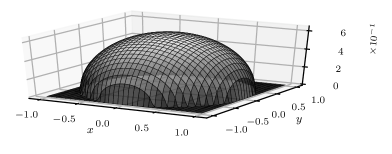
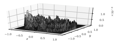
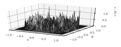
We perform numerical experiments for . Define the triangulation of the square consisting of the four triangles given by drawing diagonals. Let be the level- triangulation given by recursively dividing triangles into four (using midpoints of edges). We apply WOS to the vertices within the unit ball and define via multilevel Monte Carlo (see Eq. 3.1), using piecewise-linear interpolants of sample averages to define on the triangulation . The parameters for this algorithm are the coursest level , the finest level , and the tolerance . As test cases, we recall two examples on the unit ball where exact solutions are known (e.g., [Buc15]).
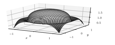
Example 3.13.
The problem with constant right-hand side and zero exterior condition on the unit ball,
has exact solution
The solution gives the mean first-exit time for an -stable Levy process from . It is plotted in Figure 1 for , along with the error from the WOS approximation with , , and .
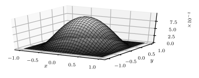
Example 3.14.
The problem
for has exact solution
| (3.16) |
For , the solution is plotted in Figure 2 along with the error for , , and .
The third example has less regular coefficients and there is no explicit exact solution.
Variance decay rates
We compute the variance decay rates for the coupling numerically, and calculate the variance at level defined by
Figure 4 shows the variance against the mesh-width and indicates decay rates for Example 3.13 independent of , and rates for Example 3.14 for . Assuming , the theoretical rate is , which yields . The rate is a good prediction in Example 3.15. For Example 3.13, the right-hand side is constant and the exterior condition is zero, which is a much simpler scenario. Due to the constant right-hand side, zero coupling-error results on the interior and improved performance can be expected, as found with the variance coupling rates of .
As a demonstration of the relative efficiency of multilevel Monte Carlo and vanilla Monte Carlo methods, LABEL:tol_cpu1 shows a plot of CPU time against tolerance. Multilevel Monte Carlo is clearly more efficient.
We can also compare the computed solution to the exact by computing an approximate norm of the error. LABEL:tab_residual shows errors for Examples 3.13 and 3.14 for seven values of and the computational time for a tolerance . Good accuracy results, especially for larger values of , and all results are computed in less than a minute on a quad-core 3.2Ghz i5-6500 CPU with 8GB RAM (three cores are used in parallel for the WOS samples). Small values of give poorer results. This is to be expected, due the sharp gradient near the border (see Eq. 3.16), which is explained by a larger constant in Theorem 3.3.
figure]tol_cpu1
| Example 3.13 | |||
|---|---|---|---|
| rel error | abs err | cpu time | |
| 0.1 | 0.079 | 0.13 | 1.9 |
| 0.2 | 0.064 | 0.10 | 2.8 |
| 0.5 | 0.034 | 0.051 | 3.6 |
| 1.0 | 0.014 | 0.018 | 5.9 |
| 1.5 | 0.008 | 0.0090 | 17.0 |
| 1.8 | 0.00081 | 0.0085 | 36.6 |
| 1.9 | 0.0062 | 0.0065 | 60.0 |
| Example 3.14 | |||
|---|---|---|---|
| rel error | abs err | cpu time | |
| 0.1 | 0.0093 | 0.0093 | 17.9 |
| 0.2 | 0.0057 | 0.0056 | 1.60 |
| 0.5 | 0.0057 | 0.0054 | 2.54 |
| 1.0 | 0.0058 | 0.0052 | 8.73 |
| 1.5 | 0.0090 | 0.0075 | 17.79 |
| 1.8 | 0.0084 | 0.0068 | 40.47 |
| 1.9 | 0.0085 | 0.0068 | 68.37 |
table]tab_residual
4 Leading eigenvalue using the Arnoldi algorithm
The Arnoldi algorithm is a well-known iterative method for computing the leading eigenvalues of a large sparse matrix, based on projecting the matrix onto a Krylov subspace. See [Arn51, TB97, CBS03, Saa11]. We show how to use Arnoldi to compute the smallest eigenvalue of the fractional Laplacian. That is, we seek the smallest such that
for some non-trivial function . The first step is to discretise the fractional Laplacian and express the problem for a finite-dimensional linear operator. To do this, we consider a triangular mesh with vertices . We consider corresponding to values of a function at vertices of the mesh and the solution operator for Eq. 1.1 with and , the piecewise-linear interpolant for on the mesh . That is, for , let be the solution to on , where , and on . Then, we denote by the linear mapping from to . By applying the Arnoldi algorithm to , we find the largest eigenvalue of and hence the smallest eigenvalue of , which is the fractional Laplacian approximated on . We use this as our approximation to the smallest eigenvalue of the fractional Laplacian.
In practice, evaluating exactly is impossible and we will be using the WOS algorithm. This means we will be using the Arnoldi algorithm with inexact solves and exploiting the theory for variable-accuracy Arnoldi algorithms started by [BF00, Sim05] and developed further in [BMGS06, FS10]. It turns out that the accuracy of the solves can be reduced as the Arnoldi algorithm proceeds, without loosing accuracy on the computed eigenvalue. This leads to significant speed ups. We develop the appropriate variable accuracy criterion for the WOS solve, by establishing a criterion on the variance of the WOS solution necessary for a certain confidence interval in the computed eigenvalue.
We now describe the algorithm. Throughout, denotes the Euclidean norm.
Inexact Arnoldi iteration
To determine the smallest eigenvalue of the fractional Laplacian on a domain , choose a triangulation of the domain with vertices and consider -vectors of values at the vertices.
Algorithm 4.1.
-
1.
Choose initial unit-vector . Set .
-
2.
Evaluate , where is the error resulting from the WOS solve.
-
3.
Gram–Schmidt: for , let and compute , to produce orthogonal to the current Krylov space, given by , and coefficients for . Let and add the vector to the Krylov space. Let be the matrix with columns .
-
4.
Compute eigenvectors and eigenvalues (known as Ritz values) for the leading submatrix of the upper Hessenberg matrix . The largest eigenpair defines an approximate eigenvector for by and approximate eigenvalue .
-
5.
Increase and repeat.
For finite-dimensional problems with exact solves ( for all ), the algorithm is expected to converge as to the leading eigenpair of . In our case, the algorithm introduces errors at several stages: First, we represent the WOS solutions on a triangular mesh and the WOS algorithm must evaluate the right-hand side function everywhere on the domain . We use a piecewise-linear interpolant and this leads to an approximation error. Additionally, there is a Monte Carlo error on due to the finite number of samples. We assume the error due to linear interpolation is negligible compared to Monte Carlo error; as the size of this error is quadratic in the mesh width , this can be achieved by choosing the triangulation fine enough. For the Monte Carlo error, we develop a theory for the resulting error in the computed eigenvalue and a practical criteria for the tolerance for the WOS solve.
4.1 Choosing the WOS tolerance
To analyse the error due to the WOS solve at step , we write
where represents the error due to the th WOS solve. The right-hand side is given by the representation of in the Krylov subspace (using the entries in the Hessenberg matrix ). We determine a criterion for relating the accuracy in the WOS solve (the size of ) in terms of the desired eigenvalue accuracy. Stacking the expressions above, we have the well-known Arnoldi relation
where is the th standard basis vector in N and is the matrix of column vectors .
In the case of zero error for , the size of the eigenvalue residual is given by , which follows easily from the Arnoldi relation
by taking the inner product with the eigenvector of . For the case of inexact solves, the residual itself is not readily available and the quantity serves as a computationally convenient proxy.
For the next theorem, we will need the following non-degeneracy assumption [Sim05, (3.3)–(3.4)]. The notation refers to the smallest singular value of .
Assumption 4.2.
For , there exists an eigenpair of sufficiently close to an eigenpair of in the sense that
where , and
| , for all eigenvalues of . |
In the following theorem, we develop the accuracy criterion for the WOS solves. We use the spectral gap for : let denote the set of eigenvalues of and
| (4.1) |
where is the leading eigenvalue of . The quantity depends on the spectrum of , which is easily computable as is generally small. We also use the -algebra generated by the random variables used in the WOS solves up to step , so that the residual is -measurable. We will use the conditional expectation to average over input random variables (WOS samples from the field solves) for .
Theorem 4.3.
Let be an eigenpair of the th Hessenberg matrix of an inexact Arnoldi iteration as described in Algorithm 4.1 such that
| (4.2) |
Suppose that the eigenvalue is simple and the eigenvector is normalised, . Fix and suppose that the WOS error vector at step satisfies
Then, is an approximate eigenvector of with eigenvalue , in the sense that
| (4.3) |
where has entries satisfying
| (4.4) |
In particular, there exists an eigenvalue of such that
Proof.
For inexact solves, the Arnoldi relationship is
where the columns of are . If is an eigenpair of , then
Hence, the eigenvalue residual
| (4.5) |
The first residual corresponds to (4.2) and is monitored during the Arnoldi iteration. The second term, we refer to as the extra residual, is due to the inexact solves and we analyse that now. Following [Sim05], it can be written as
where is the spectral gap defined in Eq. 4.1. Write,
for and if Assumption 4.2 holds, and otherwise. Here the subscripts for and indicate that they are -measurable. The Cauchy–Schwarz inequality provides that
By Chebyshev’s inequality,
If Assumption 4.2 holds, the condition on the WOS error implies that
Otherwise, Hence,
Using Eq. 4.5, this implies Eq. 4.3 under the condition Eq. 4.2.
Under Assumption 4.2, [Sim05, Proposition 2.2] implies that
Here, it is important to note that is not -measurable in general and depends on the full Arnoldi run. Then,
which is Eq. 4.4. The final statement is a consequence of the Bauer–Fike theorem for normal matrices [GVL13], which says that the error in the eigenvalue is bounded by the eigenvalue residual. ∎
This theorem suggests a practical way of choosing the WOS tolerance at step in dependence on a given eigenvalue-residual tolerance , parameter , and computed residual . For , to achieve
we assume that , and choose for . Then,
For the th WOS solve, from Theorem 4.3, we demand that
This leads to a relaxed accuracy condition for the WOS calculation if the computed eigenvalue residual is smaller than the spectral gap . It is simple to implement and requires computing the spectrum of the Hessenberg matrix at each step (to determine ) and monitoring the variance in the WOS Monte Carlo calculation.
4.2 Leading eigenvalue on the unit ball
Dyda [Dyd12] provides upper and lower bounds on the leading eigenvalue for the fractional Laplacian on the unit ball, gained by rigorous analytical methods. We compare this to the eigenvalues computed by Algorithm 4.1. Table 2 shows the results of a computation with , , and WOS multilevel parameters , and with five Arnoldi iterations. The Arnoldi iteration produces estimates that are very close to Dyda’s upper bound (the error relative to the upper bound are in the range to ). The computations take between take fifteen and thirty minutes for a Julia implementation on a quad-core 3.2Ghz i5-6500 CPU with 8GB RAM (three cores are used in parallel for the WOS samples). The run times are compared in Figure 6 to the Arnoldi algorithm without variable accuracy, taking the same tolerance in both runs. The variable accuracy algorithm is twice as fast, for the same level of accuracy.
| Dyda eigenvalue | Arnoldi | error relative | ||||
|---|---|---|---|---|---|---|
| lower bound | upper bound | eigenvalue | residual | seconds | to upper bound | |
| 0.1 | 1.04874 | 1.05096 | 1.05187 | 0.0672 | 885 | |
| 0.2 | 1.10549 | 1.10993 | 1.11103 | 0.0896 | 933 | |
| 0.5 | 1.3313 | 1.34374 | 1.34464 | 0.8147 | 838 | |
| 1.0 | 1.96349 | 2.00612 | 2.00689 | 0.095 | 907 | |
| 1.5 | 3.13569 | 3.27594 | 3.27789 | 0.017 | 1008 | |
| 1.8 | 4.28394 | 4.56719 | 4.57029 | 0.014 | 1268 | |
| 1.9 | 4.77496 | 5.13213 | 5.13936 | 0.00075 | 1711 | |
5 Conclusion
We have discussed Walk Outside Spheres for simulating the whole field rather than a point value of the solution of Eq. 1.1, extending the algorithm of [KOS17]. By using the multilevel Monte Carlo algorithm, we improved substantially on a naive method based on independent sampling at vertices. The improvement is demonstrated analytically (an improvement in the complexity for accuracy of factor where . The parameters lie in the range and are generally unknown; numerical examination of the relevant assumptions shows that can be chosen close to one and depends on ( may be chosen close to one for small and must be reduced substantially as ). The improvement is also demonstrated numerically, by looking at two problems with exact solutions and a third problem where variance estimates were made. Numerical experiments show the complexity bounds are pessimistic, even for . This is because the assumptions and analysis are based on a pair of coupled WOS processes, while the error depends on an average over a WOS path for each initial vertex.
There are several deterministic approaches to the numerical approximation of the exterior-value problem for the fractional Laplacian [LPG+18]. We compare our results to the complexity and error analysis for the adaptive finite-element method (AFEM) of [AG17, Ainsworth2018-oo]. By using a posterioi error estimates and sparse approximations to the dense linear systems resulting from the global coupling in the fractional Laplacian, it converges in the sense in two dimensions with , where is the number of degrees of freedom. Due to the use of a clustering technique in assembly of the linear system, the solution can be computed in operations. In terms of an accuracy of , this method requires operations on a polygonal domain in two dimensions (for any ). In contrast, the WOS field method on a uniform mesh takes operations to achieve a root-mean-square accuracy of , where is given in Corollary 3.12.
Though AFEM is one order of magnitude faster, the field WOS method has significant potential. First, the WOS method is trivial to parallelise and this means the constant associated to the complexity analysis can be made small, given sufficient parallel resources. This can be very significant in practical situations. Second, the WOS method developed here is a classical Monte Carlo method, depending on a sequence of independent samples from certain probability distributions. The complexity of such methods depends on the sampling error from independent samples, even for multilevel Monte Carlo methods. Very often, the complexity is substantially improved by employing quasi-Monte Carlo techniques. In situations where the sample depends on an infinite number of random variables and the importance of these random variables decays suitably rapidly, the error can be replaced by , for [HW00, GKN+11]. This sort of analysis has not been completed for the field WOS method and is beyond the scope of the present paper. It is worth noting that each sample depends on a finite but unbounded number of random variables (depending on the number of steps for the WOS path to exit the domain), but only one set of random variables is used for each vertex in the mesh (due to coupling) and the importance of these random variables decays geometrically (as the exit time is geometrically distributed [KOS17]). It will be a subject of future research to develop a quasi-Monte Carlo-based field-WOS method with improved complexity. If the is replaced by in the complexity analysis, the overall complexity improves by a factor . There is a potential also to improve the method by using an adaptive mesh. At this point, the method becomes competitive with AFEM. If these issues can be overcome, a larger class of particle methods for solving PDEs can be coupled in the same way to give efficient field solvers.
Finally, we used the WOS algorithm to compute the leading eigenvalue of the fractional Laplacian. We developed a criterion for accuracy at the th Arnoldi iteration based on the spectral gap of the Hessenberg matrix and the residual. The method is shown to give accurate results by comparing to analytical results of [Dyd12]. This algorithm can be developed further to get more leading eigenvalues and to incorporate the implicitly restarted Arnoldi method. Note the shift strategy (i.e., solving for for a shift value commonly used in eigenvalue solvers is not easy to apply with WOS; the implicitly restarted Arnoldi algorithm allows shifts to be introduced implicitly and only solves for the fractional Laplacian are required. Here again variable accuracy strategies are available [FS10] and could be adapted to the randomly inexact inner solves. This is the subject of future work.
Appendix A On Assumptions 3.5 and 3.9
We verify that Assumptions 3.5 and 3.9 are realistic, by computing the relevant quantities numerically for a square domain. For some and , we wish to establish that
and
If we replace by for the diameter of , it is clear both conditions are invariant to rescaling the domain. Hence, we focus on a box . We compute the values by a simple Monte Carlo method using , for and .
The expression for involves one parameter but must be checked for every pair of . We draw twenty independently from and evaluate using samples of and record the maximum value. We show a plot of against for in Figure 7. The condition is satisfied with for small. For larger values of , must be reduced; for example, for , must be reduced to .
The expression for involves two parameters , and we expect the appropriate choice of to depend on and for as . Again, we evaluate based on samples and Table 3 shows the result of for different choice of and . By choice of , we can always achieve for .
| 0.5 | 1.0 | 0.53 | |
| 1.0 | ⋮ | 1.03 | |
| 1.5 | 0.9 | 3.55 | |
| 1.5 | 0.5 | 0.86 | |
| 1.8 | ⋮ | 0.93 | |
| 1.5 | 0.9 | 0.85 | |
| 1.8 | ⋮ | 0.94 |
References
- [AG17] Mark Ainsworth and Christian Glusa. Aspects of an adaptive finite element method for the fractional Laplacian: A priori and a posteriori error estimates, efficient implementation and multigrid solver. Comput. Methods Appl. Mech. Eng., 327:4–35, December 2017.
- [Arn51] W. E. Arnoldi. The principle of minimized iterations in the solution of the matrix eigenvalue problem. Quarterly of Applied Mathematics, 9(1):17–29, 1951. doi: 10.1090/qam/42792.
- [BF00] A. Bouras and V. Frayssé. A relaxation strategy for inexact matrix-vector products for Krylov methods. CERFACS TR0PA000015, European Centre for Research and Advanced Training in Scientific Computation, 2000.
- [BGR61] R. M. Blumenthal, R. K. Getoor, and D. B. Ray. On the distribution of first hits for the symmetric stable processes. Trans. Amer. Math. Soc., 99(3):540–554, 1961. doi: 10.2307/1993561.
- [BMGS06] J. Berns-Müller, I. G. Graham, and A. Spence. Inexact inverse iteration for symmetric matrices. Linear Algebra Appl., 416(2):389–413, 2006. doi: 10.1016/j.laa.2005.11.019.
- [BS08] S. C. Brenner and L. R. Scott. The Mathematical Theory of Finite Element Methods. Texts in Applied Mathematics. Springer, 2008. doi: 10.1007/978-0-387-75934-0.
- [Buc15] C. Bucur. Some observations on the Green function for the ball in the fractional Laplace framework. Commun. Pure Appl. Anal., (2):657–699, February 2015. doi: 10.3934/cpaa.2016.15.657.
- [CBS03] A. W. Craig, J. F. Blowey, and T. Shardlow. Frontiers in Numerical Analysis: Durham 2002. Springer, 2003. doi: 10.1007/978-3-642-55692-0.
- [Dyd12] B. Dyda. Fractional calculus for power functions and eigenvalues of the fractional Laplacian. Fractional Calculus and Applied Analysis, 15(4):536–555, 2012. doi: 10.2478/s13540-012-0038-8.
- [FS10] M. A. Freitag and A. Spence. Shift-Invert Arnoldi’s method with preconditioned iterative solves. SIAM J. Matrix Anal. Appl., 31(3):942–969, 2010. doi: 10.1137/080716281.
- [Gil15] M. B. Giles. Multilevel Monte Carlo methods. Acta Numer., 24:259, 2015. doi: 10.1017/S096249291500001X.
- [GKN+11] I G Graham, F Y Kuo, D Nuyens, R Scheichl, and I H Sloan. Quasi-Monte Carlo methods for elliptic PDEs with random coefficients and applications. J. Comput. Phys., 230(10):3668–3694, 2011.
- [GVL13] G. H. Golub and C. F. Van Loan. Matrix Computations. Johns Hopkins University Press, Baltimore, 4th edition, 2013.
- [HW00] F J Hickernell and H Woźniakowski. Integration and approximation in arbitrary dimensions. Adv. Comput. Math., 12(1):25, January 2000.
- [KOS17] A. E. Kyprianou, A. Osojnik, and T. Shardlow. Unbiased walk-on-spheres Monte Carlo methods for the fractional Laplacian. IMA J. Numer. Anal., August 2017. doi: 10.1093/imanum/drx042.
- [LPG+18] A. Lischke, G. Pang, M. Gulian, F. Song, C. Glusa, X. Zheng, Z. Mao, W. Cai, M. M. Meerschaert, M. Ainsworth, and G. E. Karniadakis. What is the fractional Laplacian? January 2018. arXiv: 1801.09767.
- [OS17] A. Osojnik and T. Shardlow. MATLAB code for walk on spheres for fractional Laplacian. 2017. doi: 10.5281/zenodo.220877.
- [ROS16] X. Ros-Oton and J. Serra. Regularity theory for general stable operators. J. Differ. Equ., 260(12):8675–8715, 15 June 2016. doi: 10.1016/j.jde.2016.02.033.
- [Saa11] Y. Saad. Numerical Methods for Large Eigenvalue Problems: Revised Edition. SIAM, January 2011. doi: 10.1137/1.9781611970739.
- [Sim05] V. Simoncini. Variable accuracy of matrix-vector products in projection methods for eigencomputation. SIAM J. Numer. Anal., 43(3):1155–1174, 2005. doi: 10.1137/040605333.
- [TB97] L. N. Trefethen and D. Bau. Numerical Linear Algebra. SIAM, 1997. doi: 10.1137/1.9780898719574.