Multigrid preconditioners for the Newton-Krylov method in the optimal control of the stationary Navier-Stokes equations

Abstract

The focus of this work is on the construction and analysis of optimal-order multigrid preconditioners to be used in the Newton-Krylov method for a distributed optimal control problem constrained by the stationary Navier-Stokes equations. As in our earlier work [7] on the optimal control of the stationary Stokes equations, the strategy is to eliminate the state and adjoint variables from the optimality system and solve the reduced nonlinear system in the control variables. While the construction of the preconditioners extends naturally the work in [7], the analysis shown in this paper presents a set of significant challenges that are rooted in the nonlinearity of the constraints. We also include numerical results that showcase the behavior of the proposed preconditioners and show that for low to moderate Reynolds numbers they can lead to significant drops in number of iterations and wall-clock savings.

65F08, 65K15, 65N21, 65N55, 90C06

1 Introduction

We consider the optimal control problem

(1) $$\min_{y,p,u}J(y,p,u)=\frac{\gamma_{y}}{2}\|y-y_{d}\|^{2}_{\mathbf{L}^{2}(\Omega)}+\frac{\gamma_{p}}{2}\|p-p_{d}\|^{2}_{L^{2}(\Omega)}+\frac{\beta}{2}\|u\|^{2}_{\mathbf{L}^{2}(\Omega)},$$

subject to the stationary Navier-Stokes equations

(2) $$-\nu\Delta y+(y\cdot\nabla)y+\nabla p =u\quad\text{in }\Omega,$$

$$\mathrm{div}\,y =0\quad\text{in }\Omega,$$

$$y =0\quad\text{on }\partial\Omega,$$

where $\Omega\subset\mathbb{R}^{2}$ is a bounded convex polygonal domain. The goal of the control problem is to find a force $u$ that gives rise to a velocity $y$ and/or pressure $p$ to match a known target velocity $y_{d}$, respectively pressure $p_{d}$. Since this problem is ill-posed, we consider a standard Tikhonov regularization for the force, with the regularization parameter $\beta$ being a fixed positive number. The constants $\gamma_{y},\gamma_{p}$ are nonnegative, not both zero.

Model problems like (1)–(2) are commonly encountered in the literature on optimal control of partial differential equations (PDEs), where boundary conditions, forcing terms, initial values, or coefficients are treated as controls in order for the solution they determine to be close to a target state. For a given PDE-constraint, the associated control problem that is most studied is the case of distributed body forcing as control (e.g, see [32]).

Several works are centered on optimal control problems constrained by the Navier-Stokes equations, see e.g. [19, 21, 22, 11, 20, 15, 16, 12, 5] and the references therein, where both optimality conditions and numerical methods are addressed, for the unconstrained, control-constrained, or mixed control-state constrained problems. For a comprehensive overview of optimal flow control we refer the reader to [18]. In light of the potentially very large scale of the problems involved, a critical issue for all PDE-constrained optimization problems is to devise efficient solvers. These solvers largely fall into two categories: the first kind targets the sparse but indefinite Karush-Kuhn-Tucker (KKT) systems [28, 26], while the second kind is centered on reduced systems. Our strategy falls in the second category. More precisely we focus on the efficient solution of the linear systems arising in the solution process of (1)–(2), specifically on the design of multigrid preconditioners for the reduced Hessian in the Newton-CG method. To the best of our knowledge, this has not been addressed in the literature for the Navier-Stokes optimal control problem.

The multigrid preconditioning technique in this paper is rooted in the two- and multilevel methods for linear inverse problems proposed by Rieder [29], Hanke and Vogel [24], and Drăgănescu and Dupont [6], the latter being primarily concerned with regularized time-reversal of parabolic equations. The method has since been extended to distributed control of linear elliptic equations for problems with control constraints [9, 8, 10], distributed optimal control of semilinear elliptic equations [30], distributed optimal control of linear parabolic equations [23], as well as boundary control of elliptic equations [23].

The research in this article extends our earlier work on the distributed optimal control of the Stokes equations [7]; essentially, we show that for low to moderate Reynolds numbers the constructed preconditioners display the same optimal behavior as in the case of the Stokes-constrained problem. The fundamental departure from [7] resides, of course, in the nonlinearity of the constraints. Due to the linearity of the Stokes equations in [7], the cost functional of the reduced system is quadratic; thus the Hessian operator, and hence the preconditioner, is independent of the control. Instead, for the problem (1)–(2), the Hessian depends on the control, and the preconditioner changes at every Newton iteration accordingly. While the construction of the preconditioner is a natural extension of the one in [7], the main contribution in this paper lies in the analysis. The key element of the analysis is the estimation of the $\mathbf{L}^{2}$-operator norm of the difference between the discrete Hessian and the two-grid preconditioner, as expressed in the main results of this paper, Theorems 4.1 and 4.12. Due to the nonlinearity of the constraints, the discrete and continuous Hessians of the reduced cost functionals for (1)–(2) are more involved than in [7], and hence the necessary error estimates leading to the aforementioned results are more challenging. By comparison, the transition from linear elliptic to semilinear elliptic constraints [30] was facilitated by the existence of $L^{\infty}$-estimates for the control-to-state operator. The merit of our analysis is that we were able to avoid $\mathbf{L}^{\infty}$ and $\mathbf{W}_{1}^{\infty}$-estimates for the Navier-Stokes equations and its linearization which are more restrictive [13]. For convenience, the analysis is restricted to two dimensional domains, though most of it can be extended to three dimensions with some restrictions on the discretization, at least for the case of velocity control ($\gamma_{p}=0$). The preconditioning formulation can be used without change for three-dimensional problems, since it is based on a velocity-pressure formulation.

The paper is organized as follows. In Section 2, we introduce the reduced optimal control problem and review a set of results that will be needed in the sequel. In Section 3, we introduce the discrete optimal control problem and discuss finite element estimates that will be needed for the multigrid analysis. Section 4 contains the analysis of the two-grid preconditioner and the main results of the paper. In Section 5, we showcase numerical experiments that illustrate our theoretical results. Conclusions and a discussion of possible extensions are presented in Section 6.

2 Problem formulation

2.1 Preliminaries

In this section we introduce notations and review some classical existence, uniqueness, and regularity results regarding the Navier-Stokes equations which will allow to formulate the reduced form (15) of (1)–(2), and will play an essential role in the analysis. We use standard notation for the Sobolev spaces $H^{m}(\Omega)$ and for their vector-valued counterparts we use the boldface notation. We denote by $\tilde{\mathbf{H}}^{-m}(\Omega)$ the dual (with respect to $\mathbf{L}^{2}$-inner product) of $\mathbf{H}^{m}(\Omega)\cap\mathbf{H}_{0}^{1}(\Omega)$ and define $Q=L_{0}^{2}(\Omega)=\{p\in L^{2}(\Omega):\int_{\Omega}p\,dx=0\}$, $X=\mathbf{H}_{0}^{1}(\Omega)$, and $V=\{v\in\mathbf{H}^{1}_{0}(\Omega):(\mathrm{div}\,v,q)=0,\ \forall q\in Q\}$. Throughout this paper we write $(\cdot,\cdot)$ for the inner product in $L^{2}(\Omega)$ or $\mathbf{L}^{2}(\Omega)$, according to context, if there is no risk of misunderstanding. The $\mathbf{H}^{m}(\Omega)$ or $H^{m}(\Omega)$-norm will be denoted by $\|\cdot\|_{m}$, while $\|\cdot\|$ denotes the $\mathbf{L}^{2}(\Omega)$ or $L^{2}(\Omega)$-norm. Furthermore, define the norm in $V^{\prime}$ by

$$\|u\|_{V^{\prime}}=\sup_{\phi\in V\setminus\{0\}}(u,\phi)/\|\nabla\phi\|.$$

To define the weak formulation of (2), we introduce the bilinear forms

(3) $$a(y,\phi) =\nu(\nabla y,\nabla\phi)=\nu\sum_{i=1}^{2}\int_{\Omega}\nabla y_{i}\cdot\nabla\phi_{i}\,dx\quad\forall y,\phi\in X,$$

(4) $$b(\phi,p) =-\int_{\Omega}p\,\mathrm{div}\,\phi\,dx\quad\forall\phi\in X,\forall p\in Q,$$

as well as the trilinear form

(5) $$c(y;\phi,\psi)=((y\cdot\nabla)\phi,\psi)\quad\forall y,\phi,\psi\in\mathbf{H}^{1}(\Omega).$$

A weak formulation of the Navier-Stokes equations is given by:

Given $u\in\mathbf{H}^{-1}(\Omega)$, find $(y,p)\in X\times Q$ satisfying

(6) $$a(y,\phi)+c(y;y,\phi)+b(\phi,p) =\langle u,\phi\rangle\quad\forall\phi\in X,$$

$$b(y,q) =0\quad\qquad\forall q\in Q,$$

where $\langle\cdot,\cdot\rangle$ denotes the duality pairing between $\mathbf{H}_{0}^{1}(\Omega)$ and $\mathbf{H}^{-1}(\Omega)$. Following [27], the system (6) can be written equivalently as:

Find $y\in V$ that satisfies

(7) $$a(y,\phi)+c(y;y,\phi)=\langle u,\phi\rangle\quad\forall\phi\in V.$$

We recall here a standard result regarding the existence of solution of (6) and uniqueness for small data, see e.g. [14, 27]. For $\mathbf{H}^{2}$ regularity see [4].

Theorem 2.1.

Let $\Omega\subset\mathbb{R}^{2}$ be a bounded domain with Lipschitz continuous boundary. Then for any $\nu>0$ and $u\in\mathbf{H}^{-1}(\Omega)$ there exists at least one solution $(y,p)\in V\times Q$ of the stationary Navier-Stokes problem (6) that satisfies the estimate

(8) $$\|\nabla y\|\leq\nu^{-1}\|u\|_{V^{\prime}}.$$

Moreover, the solution is unique if the data satisfies the smallness condition

(9) $$\mathcal{M}\nu^{-2}\|u\|_{V^{\prime}}<1,\text{ with }\mathcal{M}=\sup_{\phi,\psi,\chi\in X\setminus\{0\}}{\frac{|c(\phi;\psi,\chi)|}{\|\nabla\phi\|\|\nabla\psi\|\|\nabla\chi\|}}.$$

If $\Omega$ is convex and polygonal, and $u\in\mathbf{L}^{2}(\Omega)$, then $y\in\mathbf{H}^{2}(\Omega)$, $p\in H^{1}(\Omega)$ and

(10) $$\|y\|_{2}+\|p\|_{1}\leq C(1+\|u\|^{3}).$$

Recall that throughout this paper we will assume $\Omega$ to be a convex polygonal domain, so that the $\mathbf{H}^{2}$-regularity of the Navier-Stokes problem is ensured. We state here some well-known results concerning the trilinear form defined in (5), that will be needed in the sequel [3, 14, 22].

Lemma 2.2.

The trilinear form $c(y;\phi,\psi)$ defined in (5) has the following properties:

(11) $$c(y;\phi,\psi)=-c(y;\psi,\phi)\quad\forall y\in V,\forall\phi,\psi\in\mathbf{H}^{1}(\Omega),$$

$$c(y;\phi,\phi)=0\quad\forall y\in V,\phi\in\mathbf{H}^{1}(\Omega),$$

$$c(y;\phi,\psi)=((\nabla\phi)^{T}\psi,y)\quad\forall y,\phi,\psi\in\mathbf{H}^{1}(\Omega),$$

$$|c(y;\phi,\psi)|\leq\|y\|_{1}\|\phi\|_{1}\|\psi\|_{1}\quad\forall y,\phi,\psi\in V,$$

$$|c(y;\phi,\psi)|\leq\mathcal{M}\|\nabla y\|\|\nabla\phi\|\|\nabla\psi\|\quad\forall y,\phi,\psi\in X,$$

$$|c(y;\phi,\psi)|\leq C\|u\|_{1}\|\phi\|_{1}\|\psi\|_{1}\quad\forall y,\phi,\psi\in\mathbf{H}^{1}(\Omega),$$

$$|c(y;\phi,\psi)|\leq C\|y\|\|\phi\|_{2}\|\psi\|_{1}\quad\forall y,\psi\in X,\phi\in\mathbf{H}^{2}(\Omega),$$

$$|c(y;\phi,\psi)|\leq C\|y\|_{1}\|\phi\|_{2}\|\psi\|\quad\forall y,\psi\in X,\phi\in\mathbf{H}^{2}(\Omega),$$

with $\mathcal{M}$ given in (9) and $C$ independent of $y,\phi,\psi$.

Proof 2.3.

While the others are standard, we prove here only the last estimate. Using Hölder’s inequality and the embedding $\mathbf{H}^{1}(\Omega)\hookrightarrow\mathbf{L}^{4}(\Omega)$, we have

$$|c(y;\phi,\psi)|=|((y\cdot\nabla)\phi,\psi)|\leq\|y\|_{L^{4}(\Omega)}\|\nabla\phi\|_{L^{4}(\Omega)}\|\psi\|_{L^{2}(\Omega)}\leq C\|y\|_{1}\|\phi\|_{2}\|\psi\|.$$

When discretizing (6) using finite elements, in order to preserve the antisymmetry in the last two arguments of the trilinear form $c$ on the finite element spaces, it is standard to introduce a modified trilinear form [21, 27]

(12) $$\tilde{c}(y;\phi,\psi)=\frac{1}{2}\{c(y;\phi,\psi)-c(y;\psi,\phi)\}\quad\forall y,\phi,\psi\in X,$$

that has the following properties:

(13) $$c(y;\phi,\psi)=\tilde{c}(y;\phi,\psi)\quad\forall y\in V,\phi,\psi\in X,$$

$$\tilde{c}(y;\phi,\psi)=-\tilde{c}(y;\psi,\phi)\quad\forall y,\phi,\psi\in X,$$

$$\tilde{c}(y;\psi,\psi)=0\quad\forall y,{\color[rgb]{0,0,0}\psi}\in X,$$

$$|\tilde{c}(y;\phi,\psi)|\leq\mathcal{M}\|\nabla y\|\|\nabla\phi\|\|\nabla\psi\|\quad\forall y,\phi,\psi\in X,$$

for the same $\mathcal{M}=\mathcal{M}(\Omega)$ as in (9). Thus, another variational formulation of (6) is:

Given $u\in\mathbf{H}^{-1}(\Omega)$, find $(y,p)\in X\times Q$ satisfying

(14) $$a(y,\phi)+\tilde{c}(y;y,\phi)+b(\phi,p) =\langle u,\phi\rangle\quad\forall\phi\in X,$$

$$b(y,q) =0\quad\qquad\forall q\in Q.$$

We define the set of admissible controls $U=\{u:\mathbf{L}^{2}(\Omega):\|u\|<\nu^{2}/(\mathcal{M}\kappa)\}$, with $\mathcal{M}$ defined in (9) and $\kappa$ the embedding constant of $\mathbf{L}^{2}(\Omega)$ into $V^{\prime}$. By Theorem 2.1, the Navier-Stokes equations have a unique solution for each $u\in U$ on the right hand side of (6). We introduce the control-to-state operators $Y:U\rightarrow V$, $P:U\rightarrow Q$ that assign to each $u\in U\subset\mathbf{L}^{2}(\Omega)$ the corresponding Navier-Stokes velocity $y=Y(u)$ and pressure $p=P(u)$, and rewrite problem (1) in reduced form as

(15) $$\min_{u\in U}\hat{J}(u)=\frac{\gamma_{y}}{2}\|Y(u)-y_{d}\|^{2}+\frac{\gamma_{p}}{2}\|P(u)-p_{d}\|^{2}+\frac{\beta}{2}\|u\|^{2}.$$

Throughout this paper we will assume that the target velocity field $y_{d}$ is from $\mathbf{H}^{1}(\Omega)$; the target pressure $p_{d}$ is assumed for now to be in $Q$.

We note that for all pairs $(y(u),u)$ with $u\in U$, we have

(16) $$\nu>\mathcal{M}(y),\quad\text{with }\mathcal{M}(y):=\sup_{v\in X}\frac{|c(v;y,v)|}{\|\nabla v\|^{2}},$$

which ensures the ellipticity of the linearized equations about $y$. The following estimate establishes the regularity of the solution of the linearized equations about $y$, and will be used in Section 4.

Lemma 2.4.

Let $u\in U$ and $y=Y(u)\in V$. Then for every $g\in V^{\prime}$ there exists a unique weak solution $(w,r)\in X\times Q$ of the linearized Navier-Stokes system

(17) $$-\nu\Delta w+(w\cdot\nabla)y+(y\cdot\nabla)w+\nabla r =g\quad\text{ in }\Omega,$$

$$\mathrm{div}\,w =0\quad\text{ in }\Omega,$$

$$w =0\quad\text{ on }\partial\Omega,$$

and

(18) $$\|\nabla w\|\leq\frac{2}{\nu}\|g\|_{V^{\prime}}.$$

If $\Omega$ is convex and polygonal, and $g\in\mathbf{L}^{2}(\Omega)$, then $w\in\mathbf{H}^{2}(\Omega)$, $r\in H^{1}(\Omega)$, and

(19) $$\|w\|_{2}\leq C(y)\|g\|.$$

Proof 2.5.

Existence and uniqueness follows from the Lax-Milgram lemma, using (16) to prove the ellipticity of the associated bilinear form. For the proof of (18) see [33], Corollary 3.7. To prove (19), we note that for $g\in\mathbf{L}^{2}(\Omega)$, we have $(w\cdot\nabla)y$, $(y\cdot\nabla)w$ $\in\mathbf{L}^{2}(\Omega)$ (see estimates below); thus by rewriting (17) as

$$-\nu\Delta w+\nabla r=g-(w\cdot\nabla)y-(y\cdot\nabla)w,$$

we can use standard regularity results for the Stokes equations to obtain

(20) $$\|\nabla\nabla w\|\leq C_{1}(\Omega)(\|g\|+\|(w\cdot\nabla)y\|+\|(y\cdot\nabla)w\|).$$

We have

$$\|(w\cdot\nabla)y\|^{2} =\int_{\Omega}|(w\cdot\nabla)y|^{2}dx\leq\int_{\Omega}|w|^{2}|\nabla y|^{2}dx\leq\|w\|^{2}_{\mathbf{L}^{4}(\Omega)}\|\nabla y\|^{2}_{\mathbf{L}^{4}(\Omega)},$$

which implies

(21) $$\|(w\cdot\nabla)y\|\leq C\|w\|_{1}\|\nabla y\|_{1}\leq C_{1}(y)\|g\|,$$

since $\mathbf{H}^{1}(\Omega)\hookrightarrow\mathbf{L}^{4}(\Omega)$. Similarly, it can be shown that

$$\|(y\cdot\nabla)w\|\leq C\|y\|_{1}\|\nabla w\|_{\mathbf{L}^{4}(\Omega)}\leq C_{2}(y)\|\nabla w\|^{1/2}\|\nabla\nabla w\|^{1/2},$$

where we used Ladyzhenskaya’s inequality,

$$\|\nabla w\|_{\mathbf{L}^{4}(\Omega)}\leq C\|\nabla w\|^{1/2}\|\nabla\nabla w\|^{1/2}.$$

Finally, using Young’s inequality we obtain

$$\|(y\cdot\nabla)w\| \leq C_{2}(y)\Big{(}\frac{1}{2}C_{2}(y)C_{1}(\Omega)\|\nabla w\|+\frac{1}{2C_{2}(y)C_{1}(\Omega)}\|\nabla\nabla w\|\Big{)}$$

$$=\frac{1}{2}C_{2}^{2}(y)C_{1}(\Omega)\|\nabla w\|+\frac{1}{2C_{1}(\Omega)}\|\nabla\nabla w\|.$$

Substituting in (20) gives

$$\|\nabla\nabla w\|\leq C_{1}(\Omega)\Big{(}\|g\|+C_{1}(y)\|g\|+\frac{1}{2}C_{2}^{2}(y)C_{1}(\Omega)\|\nabla w\|+\frac{1}{2C_{1}(\Omega)}\|\nabla\nabla w\|\Big{)},$$

from which (19) follows immediately.

We recall here the following results from [5] regarding the differentiability of the solution operators $Y$, $P$.

Theorem 2.6.

Let $u\in U$ and $y=Y(u)$. The control-to-state operators $Y$, $P$ are twice Fréchet differentiable at $u$ and their derivatives $w=Y^{\prime}(u)g$, $r=P^{\prime}(u)g$ and $\lambda=Y^{\prime\prime}(u)[g_{1},g_{2}]$, $\mu=P^{\prime\prime}(u)[g_{1},g_{2}]$ are given by the unique weak solutions of the systems:

(22) $$-\nu\Delta w+(w\cdot\nabla)y+(y\cdot\nabla)w+\nabla r =g\quad\text{ in }\Omega,$$

$$\mathrm{div}\,w =0\quad\text{ in }\Omega,$$

$$w =0\quad\text{ on }\partial\Omega,$$

and

(23) $$-\nu\Delta\lambda+(y\cdot\nabla)\lambda+(\lambda\cdot\nabla)y+\nabla\mu =-(Y^{\prime}(u)g_{1}\cdot\nabla)Y^{\prime}(u)g_{2}$$

$$\quad-(Y^{\prime}(u)g_{2}\cdot\nabla)Y^{\prime}(u)g_{1}\quad\text{in }\Omega,$$

$$\mathrm{div}\,\lambda =0\hskip 108.12047pt\text{in }\Omega,$$

$$\lambda =0\hskip 108.12047pt\text{on }\partial\Omega,$$

respectively.

Lemma 2.7.

Let $u\in U$, $y=Y(u)$, and $Y^{\prime}(u)^{*}$ be the adjoint of $Y^{\prime}(u)$. Then $z=Y^{\prime}(u)^{*}g$ is the first component of the unique weak solution $(z,\rho)$ of the system

(24) $$-\nu\Delta z-(y\cdot\nabla)z+(\nabla y)^{T}z+\nabla\rho =g\quad\text{in }\Omega,$$

$$\mathrm{div}\,z =0\quad\text{in }\Omega,$$

$$z =0\quad\text{on }\partial\Omega.$$

If $\Omega\subset\mathbb{R}^{2}$ is a convex polygonal domain then $z\in\mathbf{H}^{2}(\Omega)$, $\rho\in H^{1}(\Omega)$ and

(25) $$\|z\|_{2}\leq C(y)\|g\|.$$

Proof 2.8.

See [33, Theorem 3.10] and Lemma 2.4.

2.2 Optimality conditions

We derive next the first-order necessary optimality conditions associated with the optimal control problem (15). For $g\in\mathbf{L}^{2}(\Omega)$,

$$\hat{J}^{\prime}(u)g=\gamma_{y}(Y(u)-y_{d},Y^{\prime}(u)g)+\gamma_{p}(P(u)-p_{d},P^{\prime}(u)g)+\beta(u,g),$$

therefore

(26) $$\nabla\hat{J}(u)=\gamma_{y}Y^{\prime}(u)^{*}(Y(u)-y_{d})+\gamma_{p}P^{\prime}(u)^{*}(P(u)-p_{d})+\beta u.$$

Thus, the optimal control $u$ is the solution of the non-linear equation

(27) $$\gamma_{y}Y^{\prime}(u)^{*}(Y(u)-y_{d})+\gamma_{p}P^{\prime}(u)^{*}(P(u)-p_{d})+\beta u=0.$$

The reduced Hessian is computed using the second variation of $\hat{J}$: if $g_{1},g_{2}\in\mathbf{L}^{2}(\Omega)$

(28) $$\hat{J}^{\prime\prime}(u)[g_{1},g_{2}] =\gamma_{y}(Y^{\prime}(u)g_{2},Y^{\prime}(u)g_{1})+\gamma_{y}(Y(u)-y_{d},Y^{\prime\prime}(u)[g_{2},g_{1}])$$

$$+\gamma_{p}(P^{\prime}(u)g_{2},P^{\prime}(u)g_{1})+\gamma_{p}(P(u)-p_{d},P^{\prime\prime}(u)[g_{2},g_{1}])+\beta(g_{1},g_{2}).$$

We use different approaches in proving the main multigrid results, depending on whether the pressure term is present in the cost functional (1) or not, therefore we will derive the reduced Hessian for the two cases separately.

2.2.1 Velocity control only

We consider first the case of velocity control only, i.e., $\gamma_{y}=1,\gamma_{p}=0$. In this case the second variation of $\hat{J}$ becomes

(29) $$\hat{J}^{\prime\prime}(u)[g_{1},g_{2}] =(Y^{\prime}(u)g_{2},Y^{\prime}(u)g_{1})+(Y(u)-y_{d},Y^{\prime\prime}(u)[g_{2},g_{1}])+\beta(g_{1},g_{2}).$$

We denote by $L$ and $M$ the solution operators of (22), such that $Lg=Y^{\prime}(u)g$, $Mg=P^{\prime}(u)g$. Although $L$, $M$ depend on $y=y(u)$ in (22), we use the notation $L$, $M$ instead of $L(u)$, $M(u)$, for simplicity, when there is no risk of misunderstanding. Cf. Theorem 2.6, $\lambda=Y^{\prime\prime}(u)[g_{1},g_{2}]$ is the solution of

(30) $$a(\lambda,\phi)+c(y;\lambda,\phi) +c(\lambda;y,\phi)+b(\phi,\mu)$$

$$=-c(Lg_{1};Lg_{2};\phi)-c(Lg_{2};Lg_{1},\phi)\quad\forall\phi\in X,$$

$$b(\lambda,q) =0\hskip 147.95424pt\forall q\in Q.$$

Similarly, we let $z=L^{*}(Y(u)-y_{d})$. Note that is the solution of

(31) $$a(z,\phi)+c(y;\phi,z)+c(\phi;y,z)+b(\phi,\rho) =(y-y_{d},\phi)\quad\forall\phi\in X,$$

$$b(z,q) =0\qquad\qquad\quad\forall q\in Q.$$

By taking $\phi=z$ in (30) and $\phi=\lambda$ in (31) we obtain

(32) $$-c(Lg_{1};Lg_{2};z)-c(Lg_{2};Lg_{1},z)=(Y(u)-y_{d},\lambda).$$

Using this in (29) we get

$$\hat{J}^{\prime\prime}(u)[g_{1},g_{2}] =(Lg_{1},Lg_{2})-c(Lg_{1};Lg_{2},z)-c(Lg_{2};Lg_{1},z)+\beta(g_{1},g_{2})$$

$$=(Lg_{1},Lg_{2})+((Lg_{1}\cdot\nabla)z,Lg_{2})-((\nabla Lg_{1})^{T}z,Lg_{2})+\beta(g_{1},g_{2}).$$

The Hessian operator associated with $\hat{J}$, defined by $(H_{\beta}(u)v,g)=\hat{J}^{\prime\prime}(u)[v,g]$, is

(33) $$H_{\beta}(u)v=\beta v+L^{*}Lv+L^{*}((Lv\cdot\nabla)-(\nabla Lv)^{T})L^{*}(y-y_{d}).$$

To simplify the presentation we introduce the notation

$$A(u)v=L^{*}Lv,\quad\mathcal{C}(u)v=L^{*}((Lv\cdot\nabla)-(\nabla Lv)^{T})L^{*}(Y(u)-y_{d}),$$

that we will use throughout the paper. Note that

(34) $$(\mathcal{C}(u)v,v)=-2c(Lv;Lv,L^{*}(Y(u)-y_{d})).$$

2.2.2 Mixed/pressure control

Here we consider the general case of mixed velocity/pressure control or pressure control only, i.e, $\gamma_{p}\neq 0$.

Let $(\tilde{z},\tilde{\rho})$ be the solution of the problem

(35) $$a(\tilde{z},\phi)+c(y;\phi,\tilde{z})+c(\phi;y,\tilde{z})+b(\phi,\tilde{\rho}) =\gamma_{y}(y-y_{d},\phi)\quad\forall\phi\in X,$$

$$b(\tilde{z},q) =\gamma_{p}(p-p_{d},q)\quad\forall q\in Q,$$

which is the weak form of the problem

(36) $$-\nu\Delta\tilde{z}-(y\cdot\nabla)\tilde{z}+(\nabla y)^{T}\tilde{z}+\nabla\tilde{\rho} =\gamma_{y}(y-y_{d})\quad\text{in }\Omega,$$

$$\mathrm{div}\,\tilde{z} =\gamma_{p}(p_{d}-p)\quad\text{in }\Omega,$$

$$\tilde{z} =0\quad\qquad\qquad\text{on }\partial\Omega.$$

By taking $\phi=\lambda$ in (35), $\phi=\tilde{z}$ in (30), and using $b(\lambda,\tilde{\rho})=0$, $b(\tilde{z},\mu)=\gamma_{p}(p-p_{d},\mu)$ we obtain

$$\gamma_{y}(y-y_{d},\lambda)+\gamma_{p}(p-p_{d},\mu)=-c(Lg_{1};Lg_{2},\tilde{z})-c(Lg_{2};Lg_{1},\tilde{z}).$$

Thus, the second variation of the reduced cost functional (28) becomes

(37) $$\hat{J}^{\prime\prime}(u)[g_{1},g_{2}] =\gamma_{y}(Y^{\prime}(u)g_{2},Y^{\prime}(u)g_{1})+\gamma_{p}(P^{\prime}(u)g_{2},P^{\prime}(u)g_{1})+$$

$$\hskip 8.53581pt-c(Lg_{1};Lg_{2},\tilde{z})-c(Lg_{2};Lg_{1},\tilde{z})+{\color[rgb]{0,0,0}\beta(g_{1},g_{2})}$$

and the reduced Hessian is given by

(38) $$H_{\beta}(u)v=\beta v+\gamma_{y}L^{*}Lv+\gamma_{p}M^{*}Mv+L^{*}((Lv\cdot\nabla)\tilde{z}-(\nabla Lv)^{T}\tilde{z}).$$

We introduce the notation

(39) $$\tilde{\mathcal{C}}(u)v=L^{*}((Lv\cdot\nabla)\tilde{z}-(\nabla Lv)^{T}\tilde{z})$$

and note that

(40) $$(\tilde{\mathcal{C}}(u)v,v)=-2c(Lv;Lv,\tilde{z}).$$

Note that if we take $\gamma_{y}=1$, $\gamma_{p}=0$ in (35), then (35) is the adjoint linearized Navier-Stokes system and in this case (38) reduces to (33).

3 Discretization and approximation results

In order to discretize the optimization problem  (1)–(2) we adopt the strategy to first discretize the Navier-Stokes system, then optimize the cost functional $J$ in (1) subject to the discrete constraints.

3.1 Finite element approximation

We consider a shape regular, quasi-uniform quadrilateral mesh $\mathscr{T}_{h}$ of $\bar{\Omega}$, and we assume that the mesh $\mathscr{T}_{h}$ results from a coarser regular mesh $\mathscr{T}_{2h}$ from one uniform refinement. We use the Taylor-Hood $\mathbf{Q}_{2}-\mathbf{Q}_{1}$ finite elements to discretize the state equation. The velocity field $y$ is approximated in the space $X_{h}^{0}=X_{h}\cap\mathbf{H}_{0}^{1}(\Omega)$, where

$$X_{h} =\{v_{h}\in C(\bar{\Omega})^{2}:v_{h}|_{T}\in\mathbf{Q}_{2}(T)^{2}\text{ for }T\in\mathscr{T}_{h}\}$$

and the pressure $p$ is approximated in the space

$$Q_{h} =\{q_{h}\in C(\Omega)\cap L^{2}_{0}(\Omega):q_{h}|_{T}\in\mathbf{Q}_{1}(T)\text{ for }T\in\mathscr{T}_{h}\},$$

where $\mathbf{Q}_{k}(T)$ is the space of polynomials of degree less than or equal to $k$ in each variable [2]. The control variable $u$ is approximated by continuous piecewise biquadratic polynomial vector functions from $X_{h}$. We also introduce the space

(41) $$V_{h}=\{v_{h}\in X_{h}^{0}:(\mathrm{div}\,v_{h},q_{h})=0\ \forall q_{h}\in Q_{h}\}$$

and note that $V_{h}\nsubseteq V$.

Remark 1.

The choice to work with quadrilateral $\mathbf{Q}_{2}-\mathbf{Q}_{1}$ Taylor-Hood elements was made for convenience and clarity of exposition; our analysis can be extended to triangular $\mathbf{P}_{2}-\mathbf{P}_{1}$ elements as well as other stable mixed finite elements.

For a given control $u_{h}\in X_{h}\cap U$, the solution $(y_{h},p_{h})$ of the discrete state equation is given by

(42) $$a(y_{h},\phi_{h})+\tilde{c}(y_{h};y_{h},\phi_{h})+b(\phi_{h},p_{h}) =(u_{h},\phi_{h})\quad\forall\phi_{h}\in X_{h}^{0},$$

$$b(y_{h},q_{h}) =0\qquad\qquad\ \forall q_{h}\in Q_{h}.$$

Let $Y_{h}$ and $P_{h}$ be the solution mappings of the discretized state equation, defined analogously to their continuous counterparts. The discretized, reduced optimal control problem reads

(43) $$\min_{u_{h}}\hat{J}_{h}(u_{h})=\frac{\gamma_{y}}{2}\|Y_{h}(u_{h})-y_{d}^{h}\|^{2}+\frac{\gamma_{p}}{2}\|P_{h}(u_{h})-p_{d}^{h}\|^{2}+\frac{\beta}{2}\|u_{h}\|^{2},$$

where $y_{d}^{h},p_{d}^{h}$ are the $L^{2}$-projections of the data onto $X_{h}$, respectively $Q_{h}$.

We denote by $L_{h}$, $M_{h}$ the solution operators of the discretized linearized Navier-Stokes equations (about $y_{h}$), i.e., $L_{h}g=w_{h}$, $M_{h}g=r_{h}$, where

(44) $$a(w_{h},\phi_{h}) +\tilde{c}(y_{h};w_{h},\phi_{h})+\tilde{c}(w_{h};y_{h},\phi_{h})+b(\phi_{h},r_{h})$$

$$=(g,\phi_{h})\quad\forall\phi_{h}\in X_{h}^{0},$$

$$b(w_{h},q_{h}) =0\quad\forall q_{h}\in Q_{h},$$

We remark that, as in the continuous case, $z_{h}=L_{h}^{*}g$ satisfies

(45) $$a(z_{h},\phi_{h}) +\tilde{c}(y_{h};\phi_{h},z_{h})+\tilde{c}(\phi_{h};y_{h},z_{h})+b(\phi_{h},\rho_{h})$$

$$=(g,\phi_{h})\quad\forall\phi_{h}\in X_{h}^{0},$$

$$b(z_{h},q_{h}) =0\quad\forall q_{h}\in Q_{h}.$$

3.2 A priori estimates

In this section we collect several approximation results pertaining to the finite element approximation of the Navier-Stokes equations and the linearized/adjoint linearized Navier-Stokes equations that will be needed for the multigrid analysis.

Lemma 3.1.

Let $\pi_{h}$ be the $L^{2}$-orthogonal projection onto $X_{h}$. The following approximation properties hold:

(46) $$\|(I-\pi_{h})v\|_{\tilde{\mathbf{H}}^{-k}(\Omega)}\leq Ch^{k}\|v\|\quad\forall v\in\mathbf{L}^{2}(\Omega),\ \ k=1,2,$$

(47) $$\|(I-\pi_{h})u\|_{\tilde{\mathbf{H}}^{-1}(\Omega)}\leq Ch^{2}\|u\|_{1}\quad\forall u\in\mathbf{H}^{1}(\Omega),$$

with $C$ independent of $h$.

Proof 3.2.

The estimate (46) is a standard result (e.g., see [6]). For (47), let $I_{h}:\mathbf{H}^{1}(\Omega)\rightarrow X_{h}$ be the interpolant introduced by Scott and Zhang in [31]. We have

$$\|u-\pi_{h}u\|_{\tilde{\mathbf{H}}^{-1}(\Omega)} =\sup_{v\in\mathbf{H}^{1}_{0}(\Omega)\setminus\{0\}}\frac{(u-\pi_{h}u,v)}{\|v\|_{1}}=\sup_{v\in\mathbf{H}^{1}_{0}(\Omega)\setminus\{0\}}\frac{(u-\pi_{h}u,v-I_{h}v)}{\|v\|_{1}}$$

$$\leq\sup_{v\in\mathbf{H}^{1}_{0}(\Omega)\setminus\{0\}}\frac{\|u-\pi_{h}u\|\|v-I_{h}v\|}{\|v\|_{1}}\leq Ch\|u-\pi_{h}u\|,$$

where we have used $\|v-I_{h}v\|\leq Ch\|v\|_{1}$ (see [31, (4.6)]). Moreover,

$$\|u-\pi_{h}u\|\leq\|u-I_{h}u\|\leq ch\|u\|_{1},$$

which combined with the previous estimate leads to (47).

Theorem 3.3.

Let $u\in U$ and $y=Y(u)\in V\cap\mathbf{H}^{2}(\Omega)$ (so that $\nu>\mathcal{M}(y)$), and $L$, $M$ be the velocity/pressure operators of the linearized Navier-Stokes equations about $y$, and $L_{h}$, $M_{h}$ their discrete counterparts. There exists constants $C$, $C_{1}=C_{1}(y)$, $C_{2}=C_{2}(y)$, and $C_{3}=C_{3}(y)$ such that the following hold:

1. smoothing:

   (48) $$\|Lv\|\leq C_{1}\|v\|_{\tilde{\mathbf{H}}^{-2}(\Omega)}\quad\forall v\in\mathbf{L}^{2}(\Omega),$$

   (49) $$\|Mv\|\leq C_{2}\|v\|_{\tilde{\mathbf{H}}^{-1}(\Omega)}\quad\forall v\in\mathbf{L}^{2}(\Omega).$$

2. approximation:

   (50) $$\|Y(u)-Y_{h}(u)\|\leq Ch^{2}\|u\|\quad\forall u\in U,$$

   (51) $$\|Lv-L_{h}v\|_{1}\leq C_{1}h\|v\|\quad\forall v\in\mathbf{L}^{2}(\Omega),$$

   (52) $$\|Lv-L_{h}v\|\leq C_{1}h^{2}\|v\|\quad\forall v\in\mathbf{L}^{2}(\Omega),$$

   (53) $$\|Mv-M_{h}v\|\leq C_{2}h\|v\|\quad\forall v\in\mathbf{L}^{2}(\Omega),$$

   (54) $$\|L^{*}v-L_{h}^{*}v\|_{1}\leq C_{3}h\|v\|\quad\forall v\in\mathbf{L}^{2}(\Omega),$$

   (55) $$\|L^{*}v-L_{h}^{*}v\|\leq C_{3}h^{2}\|v\|\quad\forall v\in\mathbf{L}^{2}(\Omega),$$

3. stability:

   (56) $$\|Y_{h}(u)\|\leq C\|u\|\quad\forall u\in U,$$

   (57) $$\|L_{h}v\|\leq C_{1}\|v\|\quad\forall v\in\mathbf{L}^{2}(\Omega),$$

   (58) $$\|M_{h}v\|\leq C_{2}\|v\|\quad\forall v\in\mathbf{L}^{2}(\Omega),$$

   (59) $$\|L^{*}_{h}v\|\leq C_{3}\|v\|\quad\forall v\in\mathbf{L}^{2}(\Omega).$$

Proof 3.4.

The statement at (a) is similar to the case of the Stokes problem [7]. For (50) in (b) see [17], page 32, and for (51)–(55) see [19]. The stability in (c) follows from (8), (a), and (b).

Remark 2.

Theorem 3.3 and Lemma 3.1 imply that there is a constant $C>0$ independent of $h$ such that

(60) $$\|L(I-\pi_{h})v\|\leq Ch^{2}\|v\|\quad\forall v\in\mathbf{L}^{2}(\Omega)$$

and

(61) $$\|M(I-\pi_{h})v\|\leq Ch\|v\|\quad\forall v\in\mathbf{L}^{2}(\Omega).$$

For a polygonal domain $\Omega\subset\mathbb{R}^{2}$, the weighted Sobolev space $W_{0}^{1,0}(\Omega)$ is defined to be the class of functions for which the following norm is finite:

$$\|w\|^{2}_{W_{0}^{1,0}(\Omega)}=\int_{\Omega}|\nabla w|^{2}dx+\int_{\Omega}\delta(x)^{-2}|w|^{2}dx,$$

where $\delta(x)=\min\{\textrm{dist}(x,P):P\textrm{ a vertex of }\Omega\}.$ The following regularity and approximation result plays an important role in the analysis from Section 4.

Theorem 3.5.

Let $\Omega\subset\mathbb{R}^{2}$ be a convex polygonal domain, $u\in U$, $y=Y(u)\in V$ and $f\in\mathbf{L}^{2}(\Omega)$, $g\in W_{0}^{1,0}(\Omega)$, $\int_{\Omega}gdx=0$. Furthermore, let $\tilde{z}=\tilde{L}(f,g)$, $\tilde{\rho}=\tilde{M}(f,g)$ be the weak solution of

(62) $$-\nu\Delta\tilde{z}-(y\cdot\nabla)\tilde{z}+(\nabla y)^{T}\tilde{z}+\nabla\tilde{\rho} =f\quad\text{in }\Omega,$$

$$\mathrm{div}\,\tilde{z} =g\quad\text{in }\Omega,$$

$$\tilde{z} =0\quad\text{on }\partial\Omega.$$

Then $\tilde{z}\in\mathbf{H}^{2}(\Omega)$, $\tilde{\rho}\in H^{1}(\Omega)$ and there exists a constant $C=C(\Omega,y)>0$ such that

(63) $$\|\tilde{z}\|_{\mathbf{H}^{2}(\Omega)}+\|\nabla\tilde{\rho}\|\leq C(\|f\|_{\mathbf{L}^{2}(\Omega)}+\|g\|_{W_{0}^{1,0}(\Omega)}).$$

Moreover, if $\tilde{z}_{h}$ is the velocity of the corresponding discrete problem, then

(64) $$\|\tilde{z}-\tilde{z}_{h}\|_{1}\leq Ch(\|f\|_{\mathbf{L}_{2}(\Omega)}+\|g\|_{W_{0}^{1,0}(\Omega)}),\quad\|\tilde{z}_{h}\|_{1}\leq C(\|f\|_{\mathbf{L}_{2}(\Omega)}+\|g\|_{W_{0}^{1,0}(\Omega)}).$$

Proof 3.6.

The existence of a unique solution $(\tilde{z},\tilde{\rho})\in X\times Q$ of (62) and the estimate

(65) $$\|\tilde{z}\|_{\mathbf{H}^{1}(\Omega)}+\|\tilde{\rho}\|\leq C(\|f\|_{-1}+\|g\|),\,$$

follow from standard results for saddle point problems [1]. In [25], it is shown that under the hypotheses of the theorem, the solution of the generalized Stokes system

$$-\nu\Delta z+\nabla\rho =f\quad\text{in }\Omega,$$

$$\mathrm{div}\,z =g\quad\text{in }\Omega,$$

$$z =0\quad\text{on }\partial\Omega,$$

satisfies $z\in\mathbf{H}^{2}(\Omega)$, $\rho\in H^{1}(\Omega)$ and

$$\|z\|_{\mathbf{H}^{2}(\Omega)}+\|\nabla\rho\|\leq C(\|f\|+\|g\|_{{\color[rgb]{0,0,0}W_{0}^{1,0}(\Omega)}}).$$

Using this result together with (65), it is straightforward to show (63) using the same approach as in Lemma 2.4. For finite element spaces $X_{h},Q_{h}$ that satisfy the inf-sup condition, we have

$$\|\tilde{z}-\tilde{z}_{h}\|_{\mathbf{H}^{1}(\Omega)}+\|\tilde{\rho}-\rho_{h}\|\leq C(\inf_{\phi_{h}\in X_{h}}\|\tilde{z}-\phi_{h}\|_{\mathbf{H}^{1}(\Omega)}+\inf_{q_{h}\in Q_{h}}\|\tilde{\rho}-q_{h}\|),$$

which combined with interpolation estimates yields (64).

4 Two-grid preconditioner

In this section we present the construction of the two-grid preconditioners for the velocity control and mixed/pressure control problems, and their analyses. The main results of this paper are Theorems 4.1 and 4.12 and their Corollaries 3 and 4. We begin with the description of the discrete Hessians for the two problems in Section 4.1, followed by the construction and analysis of the two-grid preconditioners in Section 4.2. The velocity control and mixed/pressure control are treated separately, as the form of the Hessian differs significantly in the two cases.

4.1 The discrete Hessian

The discrete Hessian operator at $u\in U\cap X_{h}$ is defined by the equality

(66) $$(H_{\beta}^{h}(u)v,g)=\hat{J}_{h}^{\prime\prime}(u)[v,g],\quad\forall v,g\in X_{h}.$$

4.1.1 Velocity control

As in the continuous case, when $\gamma_{p}=0$ we have

(67) $$\nabla\hat{J}_{h}(u)=Y_{h}^{\prime}(u)^{*}(Y_{h}(u)-y_{d}^{h})+\beta u,\quad u\in U\cap X_{h},$$

with the second variation of the discrete cost functional being given by

(68) $$\hat{J}_{h}^{\prime\prime}(u)[g_{1},g_{2}] =(Y_{h}^{\prime}(u)g_{2},Y_{h}^{\prime}(u)g_{1})+(Y_{h}(u)-y_{d}^{h},Y_{h}^{\prime\prime}(u)[g_{2},g_{1}])+\beta(g_{1},g_{2}).$$

The second variation $\lambda_{h}=Y^{\prime\prime}_{h}(u)[g_{1},g_{2}]\in X_{h}^{0}$ is the solution of

(69) $$a(\lambda_{h},\phi_{h}) +\tilde{c}(y_{h};\lambda_{h},\phi_{h})+\tilde{c}(\lambda_{h};y_{h},\phi_{h})+b(\phi_{h},\mu_{h})$$

$$=-\tilde{c}(Y_{h}^{\prime}(u)g_{1};Y_{h}^{\prime}(u)g_{2},\phi_{h})-\tilde{c}(Y_{h}^{\prime}(u)g_{2};Y_{h}^{\prime}(u)g_{1},\phi_{h})\quad\forall\phi_{h}\in X_{h}^{0},$$

$$b(\lambda_{h},q_{h}) =0\quad\forall q_{h}\in Q_{h}.$$

The discrete adjoint $z_{h}=Y^{\prime}_{h}(u)^{*}(y_{h}-y_{d}^{h})=L_{h}^{*}(Y_{h}(u)-y_{d}^{h})$ is the solution of

(70) $$a(z_{h},\phi_{h}) +\tilde{c}(y_{h};\phi_{h},z_{h})+\tilde{c}(\phi_{h};y_{h},z_{h})+b(\phi_{h},\rho_{h})$$

$$=(y_{h}-y_{d}^{h},\phi_{h})\quad\forall\phi_{h}\in X_{h}^{0},$$

$$b(z_{h},q_{h}) =0\quad\forall q_{h}\in Q_{h}.$$

Using the same approach as in the continuous case, we obtain

$$-\tilde{c}(L_{h}g_{1};L_{h}g_{2},z_{h})-\tilde{c}(L_{h}g_{2};L_{h}g_{1},z_{h})=(y_{h}-y_{d}^{h},\lambda_{h})$$

and

$$\hat{J}_{h}^{\prime\prime}(u)[g_{1},g_{2}]=(L_{h}g_{1},L_{h}g_{2})-\tilde{c}(L_{h}g_{1};L_{h}g_{2},z_{h})-\tilde{c}(L_{h}g_{2};L_{h}g_{1},z_{h})+\beta(g_{1},g_{2}).$$

Hence, the discrete Hessian is given by

(71) $$H_{\beta}^{h}(u)v=\beta v+L_{h}^{*}L_{h}v+\mathcal{C}_{h}(u)v=\beta v+A_{h}(u)v+\mathcal{C}_{h}(u)v,$$

where

(72) $$(\mathcal{C}_{h}(u)v,v)=-2\tilde{c}(L_{h}v;L_{h}v,z_{h}).$$

4.1.2 Mixed/pressure control

Similarly with the derivation in Section 2.2.2, in the case of mixed/pressure control, the discrete Hessian takes the form

(73) $$H_{\beta}^{h}(u)v=\beta v+\gamma_{y}L_{h}^{*}L_{h}+\gamma_{p}M_{h}^{*}M_{h}+\tilde{\mathcal{C}}_{h}(u)v,$$

where

(74) $$(\tilde{\mathcal{C}}_{h}(u)v,v)=-2\tilde{c}(L_{h}v;L_{h}v,\tilde{z}_{h})$$

and $\tilde{z}_{h}$ is the solution of the discrete problem (35).

4.2 Two-grid preconditioner for discrete Hessian

In this section, we construct and analyze a two-grid preconditioner for the discrete Hessian $H_{\beta}^{h}(u)$ defined in (71) and (73). The construction is a natural extension of the technique used for the optimal control of the Stokes equations in [7], and is the same for both velocity- and mixed/pressure control. Let $X_{h}=X_{2h}\oplus W_{2h}$ be the $L^{2}$-orthogonal decomposition, where we consider on $X_{h}$ the Hilbert-space structure inherited from $\mathbf{L}^{2}(\Omega)$. Let $\pi_{2h}$ be the $L^{2}$-projector onto $X_{2h}$. For $u\in U\cap X_{h}$ we define the two-grid preconditioner

(75) $$T_{\beta}^{h}(u)=H_{\beta}^{2h}(\pi_{2h}u)\pi_{2h}+\beta(I-\pi_{2h}).$$

It is worth noting that

(76) $$(T_{\beta}^{h}(u))^{-1}=(H_{\beta}^{2h}(\pi_{2h}u))^{-1}\pi_{2h}+\beta^{-1}(I-\pi_{2h}).$$

We should remark that the difference between the preconditioner in (75) and the one in [7] is given by the dependence of the Hessian on the control $u$, which forces us to choose a coarse-level control $u_{c}\in X_{2h}$ at which the coarse Hessian $H_{\beta}^{2h}(u_{c})$ in (75) is computed. The natural choice is $u_{c}=\pi_{2h}u$.

4.2.1 Analysis for the case of velocity control

To assess the quality of the preconditioner we use the spectral distance between $H_{\beta}^{h}(u)$ and $T_{\beta}^{h}(u)$ defined in [6] for two symmetric positive definite operators $T_{1},T_{2}\in\mathcal{L}(V_{h})$ as

(77) $$d_{h}(T_{1},T_{2})=\underset{w\in V_{h}\setminus\{0\}}{\sup}\Bigg{|}\ln\frac{(T_{1}w,w)}{(T_{2}w,w)}\Bigg{|}.$$

Recall that, cf. (71) and (75),

(78) $$T_{\beta}^{h}(u)=(\beta I+A_{2h}(\pi_{2h}u)+\mathcal{C}_{2h}(\pi_{2h}u))\pi_{2h}+\beta(I-\pi_{2h}).$$

The key result is the following.

Theorem 4.1.

Given $u\in U\cap X_{h}$, there exists a constant $C=C(\Omega,u,{y_{d}})$ such that

(79) $$\|(H_{\beta}^{h}(u)-T_{\beta}^{h}(u))v\|\leq Ch^{2}\|v\|\quad\forall v\in X_{h}.$$

It is noteworthy that the estimate in Theorem 4.1 is symmetric in the sense that the same norm (namely the $\mathbf{L}^{2}$-norm) appears on both sides of (79), and that the estimate is of optimal order with respect to $h$. This enables us to prove the following result.

Corollary 3.

Let $u\in U\cap X_{h}$. If $\mathcal{C}_{h}(u)$ is symmetric positive definite then

(80) $$d(H_{\beta}^{h}(u),T_{\beta}^{h}(u))\leq\frac{C}{\beta}h^{2},$$

for $h<h_{0}(\beta,\Omega,L)$.

Proof 4.2.

By Theorem 4.1,

$$\Bigg{|}\frac{(T_{\beta}^{h}(u)v,v)}{(H_{\beta}^{h}(u)v,v)}-1\Bigg{|} \leq\frac{C}{\beta}\frac{h^{2}\|v\|^{2}}{\|v\|^{2}+\beta^{-1}(\|L_{h}v\|^{2}+(\mathcal{C}_{h}(u)v,v))}\leq\frac{C}{\beta}h^{2}.$$

Assume $C\beta^{-1}h_{0}^{2}=\alpha<1$, and $0<h\leq h_{0}$. Hence $T_{\beta}^{h}(u)$ is positive definite and

$$\underset{v\in X_{h}\setminus\{0\}}{\sup}\Bigg{|}\ln\frac{(T_{\beta}^{h}(u)v,v)}{(H_{\beta}^{h}(u)v,v)}\Bigg{|} \leq\frac{|\ln(1-\alpha)|}{\alpha}\underset{v\in X_{h}\setminus\{0\}}{\sup}\Bigg{|}\frac{(T_{\beta}^{h}(u)v,v)}{(H_{\beta}^{h}(u)v,v)}\Bigg{|}$$

$$\leq\frac{|\ln(1-\alpha)|}{\alpha}\frac{C}{\beta}h^{2}\leq\frac{C}{\beta}h^{2},$$

where we also used that for $\alpha\in(0,1)$, $x\in[1-\alpha,1+\alpha]$ we have

$$\frac{\ln(1+\alpha)}{\alpha}|1-x|\leq|\ln x|\leq\frac{|\ln(1-\alpha)|}{\alpha}|1-x|.$$

Prior to presenting the proof of Theorem 4.1 we prove some preliminary lemmas.

Lemma 4.3.

Let $u\in U\cap X_{h}$ and $y=Y(u)$, $p=P(u)$, $\bar{p}=P(\pi_{2h}u)$, $\bar{y}=Y(\pi_{2h}u)$. Also, let $v\in X_{h}$ and $w=L(u)v$, $q=M(u)v$, $\bar{w}=L(\pi_{2h}u)v$, $\bar{q}=M(\pi_{2h}u)v$. Then there exists a constant $K=K(u,\nu,\Omega)>0$ such that

(81) $$|y-\bar{y}|_{1}\leq K\|u-\pi_{2h}u\|_{\tilde{\mathbf{H}}^{-1}(\Omega)},$$

(82) $$\|p-\bar{p}\|\leq Kh^{2}\|u\|_{1},$$

and a constant $C$ independent of $h$ such that

(83) $$\|w-\bar{w}\|_{1}\leq Ch^{2}\|u\|_{1}\|v\|,$$

(84) $$\|q-\bar{q}\|\leq Ch^{2}\|u\|_{1}\|v\|.$$

Proof 4.4.

Since $y$ and $\bar{y}$ are the solutions of the Navier-Stokes equations with forcing $u$, $\pi_{2h}u$, respectively, we have

$$a(y,\phi)+c(y;y,\phi)=(u,\phi)\quad\forall\phi\in V,$$

$$a(\bar{y},\phi)+c(\bar{y};\bar{y},\phi)=(\pi_{2h}u,\phi)\quad\forall\phi\in V.$$

By taking $\phi=y-\bar{y}$ and subtracting the equations we obtain

$$a(y-\bar{y},y-\bar{y})+c(y-\bar{y};y,y-\bar{y})+c(\bar{y};y-\bar{y},y-\bar{y})=(u-\pi_{2h}u,y-\bar{y}).$$

Given that $c(\bar{y};y-\bar{y},y-\bar{y})=0$, we obtain

$$\nu|y-\bar{y}|^{2}_{1} = (u-\pi_{2h}u,y-\bar{y})-c(y-\bar{y};y,y-\bar{y})$$

$$\leq \|u-\pi_{2h}u\|_{\tilde{\mathbf{H}}^{-1}}\|y-\bar{y}\|_{1}+\mathcal{M}(y)|y-\bar{y}|_{1}^{2}.$$

Since $\mathcal{M}(y)<\nu$ and $y,\bar{y}\in X=\mathbf{H}_{0}^{1}(\Omega)$, we get

$$(\nu-\mathcal{M}(y))|y-\bar{y}|^{2}_{1}\leq\|u-\pi_{2h}u\|_{\tilde{\mathbf{H}}^{-1}}\|y-\bar{y}\|_{1}\leq C\|u-\pi_{2h}u\|_{\tilde{\mathbf{H}}^{-1}}|y-\bar{y}|_{1},$$

which implies (81). From the weak formulations of the Navier-Stokes equations in $X$, with forcing $u$, $\pi_{2h}u$ respectively, we have

$$b(\phi,p-\bar{p})=(u-\pi_{2h}{u},\phi)-a(y-\bar{y},\phi)+c(\bar{y};\bar{y},\phi)-c(y;y,\phi).$$

Thus for $\phi\in X$

$$|b(\phi,p-\bar{p})| \leq\|u-\pi_{2h}u\|_{-1}\|\phi\|_{1}+\nu\|y-\bar{y}\|_{1}\|\phi\|_{1}+|c(\bar{y};y-\bar{y},\phi)+c(\bar{y}-y;y,\phi)|$$

$$\leq\|u-\pi_{2h}u\|_{-1}\|\phi\|_{1}+\nu\|y-\bar{y}\|_{1}\|\phi\|_{1}+\|y-\bar{y}\|_{1}\|\phi\|_{1}(\|\bar{y}\|_{1}+\|y\|_{1}).$$

Then, from the inf-sup condition

(85) $$\beta^{*}\|q-\bar{q}\|\leq\sup_{0\neq\phi\in X}\frac{|b(q-\bar{q},\phi)|}{\|\nabla\phi\|},$$

combined with (81), (47), we obtain

$$\|p-\bar{p}\|\leq C(\nu,u,\beta^{*})h^{2}\|u\|_{1}.$$

Recall that $(w,q)$ (resp. $(\bar{w},\bar{q})$) satisfy the linearized Navier-Stokes equations (22) about $y$ (resp. $\bar{y}$) with with forcing $v$, whose weak form in $V$ read:

(86) $$a(w,\phi)+c(w;y,\phi)+c(y;w,\phi)=(v,\phi)\quad\forall\phi\in V,$$

(87) $$a(\bar{w},\phi)+c(\bar{w};\bar{y},\phi)+c(\bar{y};\bar{w},\phi)=(v,\phi)\quad\forall\phi\in V.$$

By taking $\phi=w-\bar{w}$ in the equations above and subtracting we obtain

(88) $$-a(w-\bar{w},w-\bar{w})= c(w;y;w-\bar{w})+c(y;w,w-\bar{w})$$

$$-c(\bar{w};\bar{y},w-\bar{w})-c(\bar{y};\bar{w},w-\bar{w}).$$

We have

$$c(w;y,w-\bar{w})-c(\bar{w};\bar{y},w-\bar{w}) =c(w;y-\bar{y},w-\bar{w})+c(w-\bar{w};\bar{y},w-\bar{w})$$

$$c(y;w,w-\bar{w})-c(\bar{y};\bar{w};w-\bar{w}) =c(y-\bar{y};w,w-\bar{w}),$$

where we used $c(\bar{y};w-\bar{w},w-\bar{w})=0$ (see Lemma 2.2). Using these in (88), we obtain

$$\nu|w-\bar{w}|_{1}^{2}=|c(y-\bar{y};w;w-\bar{w})+c(w;y-\bar{y},w-\bar{w})+c(w-\bar{w};\bar{y};w-\bar{w})|.$$

From the continuity of the trilinear form $c$ and (16) we get

$$\nu|w-\bar{w}|^{2}_{1}\leq\mathcal{M}\left(|y-\bar{y}|_{1}|w|_{1}|w-\bar{w}|_{1}+|w|_{1}|y-\bar{y}|_{1}|w-\bar{w}|_{1}\right)+\mathcal{M}(\bar{y})|w-\bar{w}|^{2}_{1}$$

which leads to

$$(\nu-\mathcal{M}(\bar{y}))|w-\bar{w}|^{2}_{1}\leq 2\mathcal{M}|w|_{1}|y-\bar{y}|_{1}|w-\bar{w}|_{1}.$$

Since $\|\pi_{2h}u\|\leq\|u\|$, $\pi_{2h}u\in U$, and so $\nu-\mathcal{M}(\bar{y})>0$; hence we obtain

(89) $$|w-\bar{w}|_{1}\leq C|y-\bar{y}|_{1}|w|_{1}\overset{\eqref{equ:estlinh1},\eqref{equ:neg},\eqref{equ:esty}}{\leq}Ch^{2}\|u\|_{1}\|v\|.$$

with $C$ depending on $\nu$, $y$, $\kappa$, $\mathcal{M}$, but not on $h$. To prove (84), we consider the weak formulations of (86) and (87) in $X$

$$a(w,\phi)+c(w;y,\phi)+c(y;w,\phi)+b(q,\phi) =(v,\phi)\quad\forall\phi\in X,$$

$$a(\bar{w},\phi)+c(\bar{w};\bar{y},\phi)+c(\bar{y};\bar{w},\phi)+b(\bar{q},\phi) =(v,\phi)\quad\forall\phi\in X,$$

from which we obtain

$$b(q-\bar{q},\phi) =-a(w-\bar{w},\phi)-c(w;y,\phi)-c(y;w,\phi)+c(\bar{w};\bar{y},\phi)+c(\bar{y};\bar{w},\phi)$$

$$=-a(w-\bar{w},\phi)-c(w;y-\bar{y},\phi)-c(w-\bar{w};\bar{y},\phi)-c(y;w-\bar{w},\phi)$$

$$\qquad\hskip 51.21495pt-c(y-\bar{y};\bar{w},\phi),\quad\forall\phi\in X.$$

Thus, $\forall\phi\in X$

$$|b(q-\bar{q},\phi)|\leq C|\phi|_{1}\left(|w-\bar{w}|_{1}+|w-\bar{w}|_{1}(|y|_{1}+|\bar{y}|_{1})+|y-\bar{y}|_{1}(|w|_{1}+|\bar{w}|_{1})\right).$$

Using the inf-sup condition (85) we obtain

$$\|q-\bar{q}\| \leq C(|w-\bar{w}|_{1}+|y-\bar{y}|_{1}(|w|_{1}+|\bar{w}|_{1})+|w-\bar{w}|_{1}(|y|_{1}+|\bar{y}|_{1}))$$

$$\overset{\eqref{equ:w}}{\leq}C|y-\bar{y}|_{1}(|\bar{w}|_{1}+|w|_{1}(1+|y|_{1}+|\bar{y}|_{1}))$$

$$\leq C|y-\bar{y}|_{1}\|v\|\overset{\eqref{equ:neg},\eqref{equ:esty}}{\leq}Ch^{2}\|u\|_{1}\|v\|.$$

Lemma 4.5.

Let $u\in U\cap X_{h}$ and $y=Y(u)$, $\bar{y}=Y(\pi_{2h}u)$. Also, let $v\in X_{h}$ and $z=L^{*}(y-y_{d})$, $\bar{z}=L^{*}(\bar{y}-y_{d})$. Then there exists a constant $C=C(u,y_{d})$ independent of $h$ such that

(90) $$\|z-\bar{z}\|\leq Ch^{2}\|u\|_{1}.$$

Proof 4.6.

Recall that $z$ and $\bar{z}$ are solutions of

$$a(z,\phi)+c(y;\phi,z)+c(\phi;y,z)=(y-y_{d},\phi)\quad\forall\phi\in V$$

$$a(\bar{z},\phi)+c(\bar{y};\phi,\bar{z})+c(\phi;\bar{y},\bar{z})=(\bar{y}-y_{d},\phi)\quad\forall\phi\in V.$$

By taking $\phi=z-\bar{z}$ in the previous equations and subtracting them we obtain

$$\nu|z-\bar{z}|_{1}^{2}$$

$$\leq|(y-\bar{y},z-\bar{z})|+|c(y-\bar{y};z-\bar{z},\bar{z})|+|c(z-\bar{z};y-\bar{y},z)|+|c(z-\bar{z};\bar{y},z-\bar{z})|$$

$$\leq C_{1}\|y-\bar{y}\|_{\mathbf{H}^{-1}}|z-\bar{z}|_{1}+\|y-\bar{y}\|_{1}\|z-\bar{z}\|_{1}(\|\bar{z}\|_{1}+\|z\|_{1})+\mathcal{M}(\bar{y})|z-\bar{z}|_{1}^{2},$$

which gives

$$(\nu-\mathcal{M}(\bar{y}))|z-\bar{z}|_{1}^{2} \leq|z-\bar{z}|_{1}(C_{1}\|y-\bar{y}\|+\|y-\bar{y}\|_{1}(\|z\|_{1}+\|\bar{z}\|_{1})).$$

Hence,

$$|z-\bar{z}|_{1} \leq\|y-\bar{y}\|_{1}(C_{1}+C_{2}\|y-y_{d}\|+C_{3}\|\bar{y}-y_{d}\|)\overset{\eqref{equ:esty},\eqref{equ:neg}}{\leq}C(u,y_{d})h^{2}\|u\|_{1}$$

from which (90) follows immediately.

Lemma 4.7.

Let $u\in U\cap X_{h}$, $y=Y(u)$, $y_{h}=Y_{h}(u)$. Also, let $z=L^{*}(y-y_{d})$ and $z_{h}=L^{*}_{h}(y_{h}-y_{d}^{h})$. Then there exists $C=C(u,y_{d})$ independent of $h$ so that

(91) $$\|y_{h}-y_{d}^{h}\| \leq C(\|u\|+\|y_{d}\|_{1}),$$

(92) $$\|z-z_{h}\|_{k} \leq Ch^{2-k}\|u\|,\ \ k=0,1.$$

Proof 4.8.

We have

$$\|y_{h}-y^{h}_{d}\| \leq\|y_{h}\|+\|y_{d}\|+\|y_{d}-y_{d}^{h}\|\overset{\eqref{equ:nssta}}{\leq}C\|u\|+\|y_{d}\|+\|y_{d}-y_{d}^{h}\|$$

$$\leq C\|u\|+\|y_{d}\|+\|y_{d}-I_{h}y_{d}\|\leq C(\|u\|+\|y_{d}\|+h\|y_{d}\|_{1}).$$

For $h<1$ this leads to (91). To prove (92), recall that $z$ and $z_{h}$ satisfy (31) and (70), respectively. Let $(\bar{z}_{h},\bar{\rho}_{h})$ be the solution of

(93) $$a(\bar{z}_{h},\phi_{h}) +\tilde{c}(y_{h};\phi_{h},\bar{z}_{h})+\tilde{c}(\phi_{h};y_{h},\bar{z}_{h})+b(\phi_{h},\bar{\rho}_{h})$$

$$=(y-y_{d},\phi_{h})\quad\forall\phi_{h}\in X_{h}^{0},$$

$$b(\bar{z}_{h},q_{h}) =0\quad\forall q_{h}\in Q_{h}.$$

From (54)-(55), we have

(94) $$\|z-\bar{z}_{h}\|_{k}\leq Ch^{2-k}\|y-y_{d}\|,\ \ k=0,1.$$

By taking $\phi_{h}=z_{h}-\bar{z}_{h}$ in (70) and (93) and subtracting the equations we obtain

$$\nu|z_{h}-\bar{z}_{h}|_{1}^{2} +\tilde{c}(y_{h};z_{h}-\bar{z}_{h},z_{h}-\bar{z}_{h})+\tilde{c}(z_{h}-\bar{z}_{h};y_{h},z_{h}-\bar{z}_{h})+b(z_{h}-\bar{z}_{h},\rho_{h}-\bar{\rho}_{h})$$

$$=(y-y_{h},z_{h}-\bar{z}_{h})-(y_{d}-y_{d}^{h},z_{h}-\bar{z}_{h}),$$

which, by using (12) and $(y_{d}-y_{d}^{h},z_{h}-\bar{z}_{h})=0$, simplifies to

$$\nu|z_{h}-\bar{z}_{h}|_{1}^{2}+\tilde{c}(z_{h}-\bar{z}_{h};y_{h},z_{h}-\bar{z}_{h})=(y-y_{h},z_{h}-\bar{z}_{h}).$$

Thus,

$$\nu|z_{h}-\bar{z}_{h}|^{2}_{1}\leq\|y-y_{h}\|\|z_{h}-\bar{z}_{h}\|+\mathcal{M}(y_{h})|z_{h}-\bar{z}_{h}|_{1}^{2}.$$

Since $\nu-\mathcal{M}(y_{h})>0$, we obtain

$$\|z_{h}-\bar{z}_{h}\|_{1}\leq C\|y-y_{h}\|\stackrel{{\scriptstyle\eqref{equ:nsfe}}}{{\leq}}Ch^{2}\|u\|,$$

which combined with (94) proves the lemma.

We now present the proof of Theorem 4.1.

Proof 4.9.

Cf. (71) and (78),

$$T_{\beta}^{h}(u)-H_{\beta}^{h}(u)=A_{2h}(\pi_{2h}u)\pi_{2h}-A_{h}(u)+\mathcal{C}_{2h}(\pi_{2h}u)\pi_{2h}-\mathcal{C}_{h}(u).$$

We first estimate

(95) $$A_{2h}(\pi_{2h}u)\pi_{2h}-A_{h}(u) =[A_{2h}(\pi_{2h}u)-A(\pi_{2h}u)]\pi_{2h}+A(\pi_{2h}u)(\pi_{2h}-I)$$

$$+A(\pi_{2h}u)-A(u)+A(u)-A_{h}(u).$$

For any $v\in X_{h}$ we have

$$|(A(u)-A_{h}(u))v,v)| =|(L^{*}Lv-L_{h}^{*}L_{h}v,v)|=|\|Lv||^{2}-\|L_{h}v\|^{2}|$$

$$\leq\|(L-L_{h})v\|(\|Lv\|+\|L_{h}v\|)\leq Ch^{2}\|v\|^{2},$$

which implies

$$\|(A(u)-A_{h}(u))v\|\leq Ch^{2}\|v\|,$$

since $A(u)-A_{h}(u)$ is symmetric on $X_{h}$. Similarly, it can be shown that

$$\|(A_{2h}(\pi_{2h}u)-A(\pi_{2h}u))\pi_{2h}v\|\leq Ch^{2}\|v\|.$$

For the second term in (95) we have

$$\|A(\pi_{2h}u)(\pi_{2h}-I)v\|=\|L^{*}(\pi_{2h}u)L(\pi_{2h}u)(\pi_{2h}-I)v\|\overset{\eqref{equ:negl}}{\leq}Ch^{2}\|v\|.$$

Finally, we have

$$| (A(\pi_{2h}u)v-A(u)v,v)|=|(L^{*}(\pi_{2h}u)L(\pi_{2h}u)v-L^{*}(u)L(u)v,v)|$$

$$=|\|L(\pi_{2h}u)v\|^{2}-\|L(u)v\|^{2}|\leq\|(L(\pi_{2h}u)v-L(u)v\|(\|L(\pi_{2h}u)v\|+\|L(u)v\|)$$

$$\overset{\eqref{equ:estl}}{\leq}Ch^{2}\|u\|_{1}\|v\|,$$

which implies

$$\|(A(\pi_{2h}u)-A(u))v\|\leq Ch^{2}\|v\|.$$

Combining this with the previous estimates we obtain

(96) $$\|(A_{2h}(\pi_{2h}u)-A_{h}(u))v\|\leq Ch^{2}\|v\|.$$

Next, we estimate

(97) $$\mathcal{C}_{2h}(\pi_{2h}u)\pi_{2h}-\mathcal{C}_{h}(u) =(\mathcal{C}_{2h}(\pi_{2h}u)-\mathcal{C}(\pi_{2h}u))\pi_{2h}+\mathcal{C}(\pi_{2h}u)(\pi_{2h}-I)$$

$$\quad+\mathcal{C}(\pi_{2h}u)-\mathcal{C}(u)+\mathcal{C}(u)-\mathcal{C}_{h}(u).$$

We begin by estimating the term $\|\mathcal{C}(u)v-\mathcal{C}_{h}(u)v\|$. Let $y=Y(u)$, $y_{h}=Y_{h}(u)$, $z=L^{*}(y-y_{d})$, $z_{h}=L^{*}_{h}(y_{h}-y_{d}^{h})$. Cf. (34) and (72),

$$(\mathcal{C}(u)v,v)=-2c(Lv;Lv,z)\text{ and }(\mathcal{C}_{h}(u)v,v)=-2\tilde{c}(L_{h}v;L_{h}v,z_{h}).$$

We have $c(Lv;Lv,z)=\tilde{c}(Lv;Lv,z)$ since $Lv\in V$. Therefore,

$$|(\mathcal{C}(u)v-\mathcal{C}_{h}(u)v,v)| =|2\tilde{c}(Lv;Lv,z)-2\tilde{c}(L_{h}v;L_{h}v,z_{h})|$$

$$\leq|c(Lv;Lv,z)-c(L_{h}v;L_{h}v,z_{h})|$$

$$\quad+|c(Lv;z,Lv)-c(L_{h}v;z_{h},L_{h}v)|.$$

The first term in the inequality above can be bounded by

$$|c(L_{h}v ;L_{h}v,z_{h})-c(Lv;Lv,z)|$$

$$\leq|c((L_{h}-L)v;L_{h}v,z_{h})|+|c(Lv;L_{h}v,z_{h}-z)|+|c(Lv;z,(L_{h}-L)v|,$$

where we used $c(Lv;(L_{h}-L)v,z)=-c(Lv;z,(L_{h}-L)v)$, since $Lv\in V$.
We have

$$|c((L_{h}-L)v;L_{h}v,z_{h})|$$

$$\leq|c((L_{h}-L)v;(L_{h}-L)v,z_{h})|+|c((L_{h}-L)v;Lv,z_{h})|$$

$$\leq\|(L_{h}-L)v||_{1}\|(L_{h}-L)v\|_{1}\|z_{h}\|_{1}+\|(L_{h}-L)v\|\|Lv\|_{2}\|z_{h}\|_{1}$$

$$\overset{\eqref{equ:lnsfeh1},\eqref{equ:lnsfe}}{\leq}Ch^{2}\|v\|^{2}\|z_{h}\|_{1}\overset{\eqref{equ:alnsstab}}{\leq}Ch^{2}\|v\|^{2}\|y_{h}-y_{d}^{h}\|\overset{\eqref{equ:ydestimate}}{\leq}C(u,y_{d})h^{2}\|v\|^{2},$$

and

$$|c(Lv;L_{h}v,z_{h}-z)| \leq|c(Lv;(L_{h}-L)v,z_{h}-z)|+|c(Lv;Lv,z_{h}-z)|$$

$$\leq\|Lv\|_{1}\|(L_{h}-L)v\|_{1}\|z_{h}-z\|_{1}+C\|Lv\|_{1}\|Lv\|_{2}\|z_{h}-z\|$$

$$\overset{\eqref{equ:lnsfeh1},\eqref{equ:estlinh2},\eqref{equ:zestimate}}{\leq}Ch^{2}\|v\|^{2}\|y_{h}-y_{d}^{h}\|\overset{\eqref{equ:ydestimate}}{\leq}C(u,y_{d})h^{2}\|v\|^{2}.$$

Combining these estimates with

$$|c(Lv;z,(L_{h}-L)v)|\leq C\|Lv\|_{1}\|z\|_{2}\|(L_{h}-L)v\|\overset{\eqref{equ:regalin},\eqref{equ:lnsfe}}{\leq}C(u,y_{d})h^{2}\|v\|^{2},$$

we obtain

$$|c(L_{h}v ;L_{h}v,z_{h})-c(Lv;Lv,z)|\leq C(u,y_{d})h^{2}\|v\|^{2}.$$

Similarly,

$$|c(L_{h}v ;z_{h},L_{h}v)-c(Lv;z,Lv)|$$

$$\leq|c((L_{h}-L)v;z_{h},L_{h}v)|+|c(Lv;z_{h},(L_{h}-L)v)|+|c(Lv;Lv,z-z_{h})|$$

$$\leq|c((L_{h}-L)v;z_{h}-z,L_{h}v)|+|c((L_{h}-L)v;z,L_{h}v)|$$

$$\quad+|c(Lv;z_{h}-z,(L_{h}-L)v)|+|c(Lv;z,(L_{h}-L)v)|+|c(Lv;Lv,z-z_{h})|$$

$$\leq\|(L_{h}-L)v\|_{1}\|z_{h}-z\|_{1}\|L_{h}v\|_{1}+C\|(L_{h}-L)v\|\|z\|_{2}\|L_{h}v\|_{1}$$

$$\quad+\|Lv\|_{1}\|z_{h}-z\|_{1}\|(L_{h}-L)v\|_{1}+C\|Lv\|_{1}\|z\|_{2}\|(L_{h}-L)v\|$$

$$\quad+C\|Lv\|_{1}\|Lv\|_{2}\|z-z_{h}\|\overset{\eqref{equ:regalin},\eqref{equ:lnsfeh1},\eqref{equ:lnsfe},\eqref{equ:zestimate}}{\leq}C(u,y_{d})h^{2}\|v\|^{2}.$$

Using the same approach, it can be shown that

$$\|(\mathcal{C}_{2h}(\pi_{2h}u)-\mathcal{C}(\pi_{2h}u)\pi_{2h}v\|\leq Ch^{2}\|v\|.$$

Let $\bar{z}=L^{*}(Y(\pi_{2h}u)-y_{d})$. The third term in (97) can be bounded as

$$|(\mathcal{C}(\pi_{2h}u)v-\mathcal{C}(u)v,v)| =2|c(Lv;Lv,\bar{z})-c(Lv;Lv,z)|=2|c(Lv;Lv,\bar{z}-z)|$$

$$\leq C\|Lv\|_{1}\|Lv\|_{2}\|\bar{z}-z\|\stackrel{{\scriptstyle\eqref{equ:estlinh2}}}{{\leq}}C\|v\|^{2}\|\bar{z}-z\|$$

$$\overset{\eqref{equ:zthm}}{\leq}C(u,y_{d})h^{2}\|u\|_{1}\|v\|^{2}.$$

Finally let $w=(\pi_{2h}-I)v$. With $L=L(\pi_{2h}u)$, we have

$$|(\mathcal{C}(\pi_{2h}u)(\pi_{2h}-I)v,v)|$$

$$=|((Lw\cdot\nabla)\bar{z}-(\nabla Lw)^{T}\bar{z},Lv)|\leq|((Lw\cdot\nabla)\bar{z}),Lv)|+|(\nabla Lw)^{T}\bar{z},Lv)|$$

$$=|c(Lw;\bar{z},Lv)|+|c(Lv;Lw,\bar{z})|\overset{\eqref{equ:trilinear}}{=}|c(Lw;\bar{z},Lv)|+|c(Lv;\bar{z},Lw)|$$

$$\overset{\eqref{equ:trilinear}}{\leq}C\|Lw\|\|\bar{z}\|_{2}\|Lv\|_{1}\overset{\eqref{equ:negl}}{\leq}Ch^{2}\|v\|\|\bar{z}\|_{2}\|v\|\overset{\eqref{equ:regalin}}{\leq}C(u,y_{d})h^{2}\|v\|^{2}.$$

4.2.2 Analysis for the case of mixed/pressure control

Recall from (73) that in the case of mixed/pressure control, the discrete Hessian takes the form

$$H_{\beta}^{h}(u)v=\beta v+\gamma_{y}A_{h}v+\gamma_{p}B_{h}v+\tilde{\mathcal{C}}_{h}(u)v,$$

where $B_{h}=M_{h}^{*}M_{h}$ and $A_{h}=L_{h}^{*}L_{h}$ as in (71). Following the definition in (75), the two-grid preconditioner takes the form

(98) $$T_{\beta}^{h}(u) =(\beta I+\gamma_{y}A_{2h}(\pi_{2h}u)+\gamma_{p}B_{2h}(\pi_{2h}u)+\tilde{\mathcal{C}}_{2h}(\pi_{2h}u))\pi_{2h}+\beta(I-\pi_{2h}).$$

Lemma 4.10.

Let $u\in U\cap X_{h}$ and $y=Y(u)$, $p=P(u)$, $\bar{y}=Y(\pi_{2h}u)$, $\bar{p}=P(\pi_{2h}u)$. Also, let $v\in X_{h}$ and $\tilde{z}=\tilde{L}(\gamma_{y}(y-y_{d}),\gamma_{p}(p_{d}-p))$, $\hat{z}=\tilde{L}(\gamma_{y}(\bar{y}-y_{d}),\gamma_{p}(p_{d}-\bar{p}))$, with $\tilde{L}$ defined in Theorem 3.5. Then there exists a constant $C=C(u,y_{d},p_{d},\gamma_{y},\gamma_{p})$ independent of $h$ such that

(99) $$\|\tilde{z}-\hat{z}\|_{1}\leq Ch\|u\|_{1}^{1/2}.$$

Proof 4.11.

Recall that $(\tilde{z},\tilde{\rho})$ is the solution of (35), and $(\hat{z},\hat{\rho})$ satisfies

(100) $$a(\hat{z},\phi)+c(\bar{y};\phi,\hat{z})+c(\phi;\bar{y},\hat{z})+b(\phi,\hat{\rho}) =\gamma_{y}(\bar{y}-y_{d},\phi)\quad\forall\phi\in X,$$

$$b(\hat{z},q) =\gamma_{p}(\bar{p}-p_{d},q)\quad\forall q\in Q,$$

By subtracting (100) from (35) we obtain

$$a(\tilde{z}-\hat{z},\phi)+c(y;\phi,\tilde{z}-\hat{z}) + c(\phi;y,\tilde{z}-\hat{z})+b(\phi,\tilde{\rho}-\bar{\rho})=$$

$$\gamma_{y}(y-\bar{y})+c(\bar{y}-y;\phi,\hat{z})+c(\phi;\bar{y}-y,\hat{z})$$

$$b(\tilde{z}-\bar{z},q) = \gamma_{p}(\bar{p}-p),\ \ \forall\phi\in X,q\in Q,$$

which represents the weak form of

$$-\nu\Delta(\tilde{z}-\hat{z})-(y\cdot\nabla)(\tilde{z}-\hat{z})+(\nabla y)^{T}(\tilde{z}-\hat{z})+\nabla(\tilde{\rho}-\hat{\rho}) =\gamma_{y}(y-\bar{y})+((y-\bar{y})\cdot\nabla)\hat{z}$$

$$-(\nabla(y-\bar{y}))^{T}\hat{z}\quad\text{in }\Omega,$$

$$\mathrm{div}\,(\tilde{\rho}-\hat{\rho}) =\gamma_{p}(\bar{p}-p)\quad\text{in }\Omega$$

$$\tilde{z}-\hat{z} =0\quad\text{on }\partial\Omega.$$

Using (65), we get

(101) $$\|\tilde{z}-\hat{z}\|_{1} \leq C(\gamma_{y}\|y-\bar{y}\|+\gamma_{p}\|p-\bar{p}\|+\|((y-\bar{y})\cdot\nabla)\hat{z}\|+\|(\nabla(y-\bar{y}))^{T}\hat{z}\|).$$

From (21), combined with (81),(47),(65), we have

$$\|((y-\bar{y})\cdot\nabla)\hat{z}\|\leq C\|y-\bar{y}\|_{1}\|\nabla\hat{z}\|\leq Ch^{2}(\gamma_{y}\|\bar{y}-y_{d}\|+\gamma_{p}\|\bar{p}-p_{d}\|).$$

Of the four terms in the right hand side of (101), only the last is of order one in $h$:

$$\|(\nabla(y-\bar{y}))^{T}\hat{z}\| \leq\|\nabla(y-\bar{y})\|_{\mathbf{L}^{4}(\Omega)}\|\hat{z}\|_{\mathbf{L}^{4}(\Omega)}\leq C\|\nabla(y-\bar{y})\|^{1/2}\|\nabla\nabla(y-\bar{y})\|^{1/2}\|\hat{z}\|_{1}$$

$$\overset{\eqref{equ:h2nse},\eqref{equ:esty},{\eqref{equ:neg}},\eqref{equ:snz}}{\leq}C(u)h\|u\|_{1}^{1/2}(\|\bar{y}-y_{d}\|+\|\bar{p}-p_{d}\|).$$

Using these estimates together with (81), (82), (47) in (101) we obtain

$$\|\tilde{z}-\hat{z}\|_{1}\leq C(u)h\|u\|_{1}^{1/2}(\gamma_{y}\|\bar{y}-y_{d}\|+\gamma_{p}\|\bar{p}-p_{d}\|).$$

We are now in a position to prove the main result for mixed/pressure control.

Theorem 4.12.

Let $u\in U\cap X_{h}$ be so that $p=P(u)\in W_{0}^{1,0}(\Omega)$. If $p_{d}\in W_{0}^{1,0}(\Omega)\cap Q$, then there exists a constant $C=C(\Omega,u,y_{d},p_{d},\gamma_{y},\gamma_{p})$ such that

$$\|(H_{\beta}^{h}(u)-T_{\beta}^{h}(u))v\|\leq Ch\|v\|\quad\forall v\in X_{h}.$$

Proof 4.13.

For any $u\in U\cap X_{h}$, we have

$$T_{\beta}^{h}(u)-H_{\beta}^{h}(u) =\gamma_{y}(A_{2h}(\pi_{2h}u)\pi_{2h}-A_{h}(u))+\gamma_{p}(B_{2h}(\pi_{2h}u)\pi_{2h}-B_{h}(u))$$

$$+\tilde{\mathcal{C}}_{2h}(\pi_{2h}u)\pi_{2h}-\tilde{\mathcal{C}}_{h}(u).$$

We use the same approach as in the case of velocity control only. We have already shown in (96) that the first term is $O(h^{2}\|v\|)$. The second term is estimated similarly:

(102) $$B_{2h}(\pi_{2h}u)\pi_{2h}-B_{h}(u) =[B_{2h}(\pi_{2h}u)-B(\pi_{2h}u)]\pi_{2h}+B(\pi_{2h}u)(\pi_{2h}-I)$$

$$+B(\pi_{2h}u)-B(u)+B(u)-B_{h}(u).$$

For any $v\in X_{h}$ we have

$$|((B(u)-B_{h}(u))v,v)| =|(M^{*}Mv-M_{h}^{*}M_{h}v,v)|=|\|Mv\|^{2}-\|M_{h}v\|^{2}|$$

$$\leq\|Mv-M_{h}v\|(\|Mv\|+\|M_{h}v\|)\leq Ch\|v\|^{2},$$

where we used (53) and (58). Similarly, it can be shown

$$\|(B_{2h}(\pi_{2h}u)-B(\pi_{2h}u))v\|\leq Ch\|v\|^{2},\quad\forall v\in X_{h}.$$

The second term in (102) can be bounded as

(103) $$\|B(\pi_{2h}u)(\pi_{2h}-I)v\|=\|M^{*}(\pi_{2h}u)M(\pi_{2h}u)(\pi_{2h}-I)v\|\overset{\eqref{equ:nppl}}{\leq}Ch\|v\|.$$

Finally, we have

$$|(B(\pi_{2h}u)v -B(u)v,v)|=|(M^{*}(\pi_{2h}u)M(\pi_{2h}u)v-M^{*}(u)M(u)v,v)|$$

$$=|\|M(\pi_{2h}u)v\|^{2}-\|M(u)v\|^{2}|$$

$$\leq\|(M(\pi_{2h}u)v-M(u)v\|(\|M(\pi_{2h}u)v\|+\|M(u)v\|)\overset{\eqref{equ:estp}}{\leq}Ch^{2}\|u\|_{1}\|v\|,$$

which gives

(104) $$\|(B(\pi_{2h}u)-B(u))v\|\leq Ch^{2}\|u\|_{1}\|v\|.$$

Next, we estimate

(105) $$\tilde{\mathcal{C}}_{2h}(\pi_{2h}u)\pi_{2h}-\tilde{\mathcal{C}}_{h}(u) =[\tilde{\mathcal{C}}_{2h}(\pi_{2h}u)-\tilde{\mathcal{C}}(\pi_{2h}u)]\pi_{2h}+\tilde{\mathcal{C}}(\pi_{2h}u)(\pi_{2h}-I)$$

$$+\tilde{\mathcal{C}}(\pi_{2h}u)-\tilde{\mathcal{C}}(u)+\tilde{\mathcal{C}}(u)-\tilde{\mathcal{C}}_{h}(u).$$

We first estimate the term $\|\tilde{\mathcal{C}}(u)v-\tilde{\mathcal{C}}_{h}(u)v\|$, and recall that

$$(\tilde{\mathcal{C}}(u)v,v)=-2c(Lv;Lv,\tilde{z})\text{ and }(\tilde{\mathcal{C}}_{h}(u)v,v)=-2\tilde{c}(L_{h}v;L_{h}v,\tilde{z}_{h}),$$

with $\tilde{z}=\tilde{L}(\gamma_{y}(y-y_{d}),\gamma_{p}(p_{d}-p))$, $\tilde{z}_{h}=\tilde{L}_{h}(\gamma_{y}(y_{h}-y_{d}^{h}),\gamma_{p}(p_{d}^{h}-p_{h}))$, with the operators $\tilde{L}$ and $\tilde{L}_{h}$ as defined in Theorem 3.5. Thus,

$$|(\tilde{\mathcal{C}}(u)v-\tilde{\mathcal{C}}_{h}(u)v,v)| =|2\tilde{c}(Lv;Lv,\tilde{z})-2\tilde{c}(L_{h}v;L_{h}v,\tilde{z}_{h})|$$

$$\leq|c(Lv;Lv,\tilde{z})-c(L_{h}v;L_{h}v,\tilde{z}_{h})|$$

$$\quad+|c(Lv;\tilde{z},Lv)-c(L_{h}v;\tilde{z}_{h},L_{h}v)|.$$

The first term in the inequality above can be bounded by

$$|c(L_{h}v;L_{h}v,\tilde{z}_{h})-c(Lv;Lv,\tilde{z})| \leq|c((L_{h}-L)v;L_{h}v,\tilde{z}_{h})|+|c(Lv;L_{h}v,\tilde{z}_{h}-\tilde{z})|$$

$$\quad+|c(Lv;\tilde{z},(L_{h}-L)v|,$$

where we used $c(Lv;L_{h}v-Lv,\tilde{z})=-c(Lv;\tilde{z},L_{h}v-Lv)$ since $Lv\in V$. Thus, we have

$$|c(L_{h}v;L_{h}v,\tilde{z}_{h})-c(Lv;Lv,\tilde{z})|$$

$$\leq C(\|Lv-L_{h}v\|_{1}\|L_{h}v\|_{1}\|\tilde{z}_{h}\|_{1}+\|Lv\|_{1}\|L_{h}v\|_{1}\|\tilde{z}_{h}-\tilde{z}\|_{1}+\|Lv\|_{1}\|\tilde{z}\|_{1}\|L_{h}v-Lv\|_{1})$$

$$\stackrel{{\scriptstyle\eqref{equ:lnsfeh1},\eqref{equ:fenz}}}{{\leq}}Ch\|v\|^{2}(\gamma_{y}\|y-y_{d}\|+\gamma_{p}\|p-p_{d}\|_{W_{0}^{1,0}(\Omega)}).$$

Note that we have used (64) also for $\|L_{h}v\|_{1}\leq C\|v\|$, since $L_{h}v=\tilde{L}_{h}(v,0)$. Also,

$$|c(L_{h}v ;\tilde{z}_{h},L_{h}v)-c(Lv;\tilde{z},Lv)|\leq|c((L_{h}-L)v;\tilde{z}_{h},L_{h}v)|+|c(Lv;\tilde{z}_{h},(L_{h}-L)v)|$$

$$+|c(Lv;Lv,\tilde{z}-\tilde{z}_{h})|$$

$$\leq\|L_{h}v-Lv\|_{1}\|\tilde{z}_{h}\|_{1}\|L_{h}v\|_{1}+\|Lv\|_{1}\|\tilde{z}_{h}\|_{1}\|L_{h}v-Lv\|_{1}$$

$$+\|Lv\|_{1}\|Lv\|_{1}\|\tilde{z}-\tilde{z}_{h}\|_{1}\leq Ch\|v\|(\gamma_{y}\|y-y_{d}\|+\gamma_{p}\|p-p_{d}\|_{W_{0}^{1,0}(\Omega)}).$$

Similarly, it can be shown that $\|(\tilde{\mathcal{C}}_{2h}(\pi_{2h}u)-\tilde{\mathcal{C}}(\pi_{2h}u)\pi_{2h}v\|\leq Ch\|v\|$. To estimate the third term in (105), let $\hat{z}=\tilde{L}(\gamma_{y}(Y(\pi_{2h}u)-y_{d}),\gamma_{p}(p_{d}-P(\pi_{2h}u)))$. Then

$$|(\tilde{\mathcal{C}}(\pi_{2h}u)v-\tilde{\mathcal{C}}(u)v,v)|=2|c(Lv;Lv,\tilde{z})-c(Lv;Lv,\hat{z})|=2|c(Lv;Lv,\tilde{z}-\hat{z})|$$

$$\leq C\|Lv\|_{1}^{2}\|\tilde{z}-\hat{z}\|_{1}\stackrel{{\scriptstyle\eqref{equ:fenz}}}{{\leq}}C\|v\|^{2}\|\tilde{z}-\hat{z}\|_{1}\overset{\eqref{equ:ztildethm}}{\leq}C(u,y_{d},p_{d},\gamma_{y},\gamma_{p})h\|v\|^{2}.$$

Finally, let $w=(\pi_{2h}-I)v$. With $L=L(\pi_{2h}u)$ we have (see (39))

$$|(\tilde{\mathcal{C}}(\pi_{2h}u)(\pi_{2h}-I)v,v)|=|((Lw\cdot\nabla)\hat{z}-(\nabla Lw)^{T}\hat{z},Lv)|$$

$$\leq|((Lw\cdot\nabla)\hat{z}),Lv)|+|(\nabla Lw)^{T}\hat{z},Lv)|=|c(Lw;\hat{z},Lv)|+|c(Lv;Lw,\hat{z})|$$

$$=|c(Lw;\hat{z},Lv)|+|c(Lv;\hat{z},Lw)|\leq C\|Lw\|\|\hat{z}\|_{2}\|Lv\|$$

$$\overset{\eqref{equ:negl}}{\leq}Ch^{2}\|v\|\|\hat{z}\|_{2}\|v\|\overset{\eqref{equ:adj_nzd}}{\leq}C(u,y_{d},p_{d},\gamma_{y},\gamma_{p})h^{2}\|v\|^{2}$$

which combined with the other estimates yields the conclusion.

The following result follows from Theorem 4.12 using arguments similar to the ones in the proof of Corollary 3. Essentially it shows a decline by one unit in the approximation order of the two-grid preconditioner for the case of mixed/pressure control compared to velocity control. This is consistent with the case of the Stokes-constrained problem studied in [7].

Corollary 4.

Under the conditions of Theorem 4.12, if $\tilde{\mathcal{C}}_{h}(u)$ is symmetric positive definite then

(106) $$d(H_{\beta}^{h}(u),T_{\beta}^{h}(u))\leq\frac{C}{\beta}h,$$

for $h<h_{0}(\beta,\Omega,L,M,\tilde{L})$.

Remark 5.

We should note that the hypotheses of Theorem 4.12 are quite restrictive, in that we cannot expect $p_{d}$ and $P(u)\in W_{0}^{1,0}(\Omega)$ in practice; smooth functions in $W_{0}^{1,0}(\Omega)$ tend to zero near the corners of the domain and there is no a priori reason for a flow to have a zero-pressure near the corners of the domain. Nevertheless, this fact does not prevent the preconditioner to work quite well for the mixed/pressure control, as shown in Section 5.

Remark 6.

The two-grid preconditioner can be extended to a multigrid preconditioner following essentially the same strategy as in [7], and the analysis is extended in a similar fashion to show that the multigrid preconditioner satisfies the estimates (80) and (106). Suffice it to say that the correct multigrid preconditioner has a $W$-cycle structure, while the associated $V$-cycle gives suboptimal results; furthemore, the coarsest level has to be sufficiently fine in order for the optimal quality to be preserved.

5 Numerical results

We present a set of numerical results to showcase the behavior of our multigrid preconditioner in the Newton iteration of (43) on $\Omega=(0,1)^{2}$. We consider uniform rectangular grids with mesh sizes $h=1/32,1/64,1/128,1/256$, and we use Taylor-Hood $\mathbf{Q}_{2}$−-$\mathbf{Q}_{1}$ elements for velocity-pressure and $\mathbf{Q}_{2}$ elements for the controls. The data is given by $y_{d}^{h}=Y_{h}(u_{h})$, $p_{d}^{h}=P_{h}(u_{h})$, with $u_{h}$ being the interpolant of the target control $u(x,y)=[10^{3}(\textnormal{sign}(y-0.9)+1)(y-0.9)^{2},0]$ (see Figure 1); the velocity field resembles one obtained from a lid-driven cavity flow. In Figure 2 we show the optimal control and the recovered velocity and pressure profile for the velocity control problem. As can be seen in the picture, if $\gamma_{p}=0$, the pressure is not recovered. The Newton iteration is stopped when $\|\nabla\hat{J}_{h}\|_{\infty}\leq 10^{-10}$. On the coarsest grid at $h=1/32$ we use a zero-initial guess for the Newton solve, while for subsequent grids we start the iteration using the solution from the coarser problem. The linear systems at each iteration are solved in two ways: first we use conjugate gradient preconditioned by the multigrid preconditioner (MGCG) (see Remark 6), with base cases $h_{0}=1/32$ or $1/64$, depending on necessity. Second, we solve the same systems using unpreconditioned conjugate gradient (CG). The reduced Hessian is applied matrix-free using (71)–(73). Obviously, the Hessian-vector multiplication (matvec) is the most expensive operation, as it essentially requires solving the linearized Navier-Stokes system twice. The goal is to show that, as a result of multigrid preconditioning, the number of matvecs at the highest resolution is relatively low compared to the unpreconditioned case.

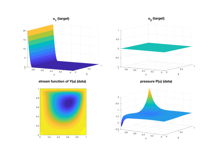
Figure 1: Top images: components of target control. Bottom images: velocity (stream function) and pressure data. Viscosity is $\nu=0.01$ with $Re=\nu^{-1}\|Y(u)\|_{\infty}\approx 105$, and $h=1/64$.

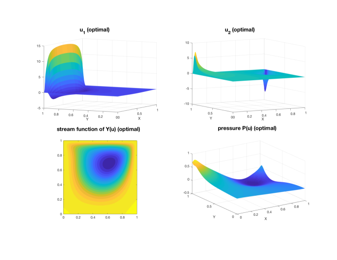
Figure 2: Top images: components of optimal control corresponding to data from Figure 1. Bottom images: optimal velocity (stream function) and pressure. Parameters values are: $\gamma_{y}=1$, $\gamma_{p}=10^{-3}$, and $\beta=10^{-5}$.

We present in Table 1 results for low and in Table 2 for moderate Reynolds numbers, and we compare velocity control ($\gamma_{p}=0$) with mixed velocity-pressure control with varying ratios of the two terms in $\hat{J}_{h}$ ($\gamma_{y}=1$, $\gamma_{p}=10^{-4},10^{-3}$). As for the regularization parameter we let $\beta=10^{-4},10^{-5}$. For each of the twelve parameter choices and for each $h=1/64,1/128,1/256$ we report the number of iterations of the MGCG/CG-based solves for each Newton iteration as well as the total (added) wall-clock time of the linear solves (since the overhead due to the gradient computation and Hessian setup is the same for both solves). For example, in the top left compartment of Table 2, we show the case $\nu=0.01$, $\gamma_{y}=1,\gamma_{p}=0$ (velocity control only), $\beta=10^{-4}$ with resolutions $1/64,1/128,1/256$. At resolution $h=1/256$ two Newton iterations were required with CG necessitating $382$ and $274$ iterations, with a total time of linear solves of $11.4$ hours, while the four-grid MGCG needed $6$ and $4$ iterations for a total of $0.58$ hours, meaning almost twenty times faster. Note that at the coarsest level we actually build the Hessian at each Newton iteration and invert it using direct methods, the time of this operation being included in the reported wall-clock time. We should note that using direct methods at the coarsest level is critical for mixed/pressure control, but can be replaced with low-tolerance iterative solves for velocity control, a phenomenon that is still under scrutiny. For the experiments in Tables 1 and 2 the relative tolerance for both CG and MGCG is set at $10^{-8}$. While this is quite low for the Newton-CG method, it forces a slightly higher number of linear iterations, thus allowing to better observe the desired behavior of the MGCG preconditioner, namely that for fixed $\beta$ the number of linear iterations will decrease with $h\downarrow 0$. For two of the twelve cases we also vary the tolerance for the linear solves ($10^{-2}$ and $10^{-4}$) and show the results in Table 3. Here we also report the total wall-clock time for the computation (including the gradient computation and Hessian setup at each Newton iteration), since the number of Newton iterations begins to vary between CG to MGCG when using a large tolerance. This is due mainly to two factors related to MGCG: either it converges very fast and the gradients are better approximated than expected even if the tolerance is set at $10^{-2}$, or the MG preconditioner is not positive definite and so MGCG fails to converge (we still report 1 MGCG iteration). We allow a maximum of 10 Newton iterations.

Tables 1 and 2 indicate a behavior that is standard for the multigrid preconditioner presented in this work, and which is consistent with the analysis. First we notice that unpreconditioned CG is scalable, in the sense that for each case the number of CG iterations is bounded with respect to mesh-size (the wall-clock times suffer due to the fact that we used direct solvers for the linearized Navier-Stoles solves in the matvec). The MGCG instead shows an efficiency that increases over CG with decreasing $h$, measured both in terms of number of iterations and wall-clock time, and this can be seen for all the velocity control cases, and for the mixed control cases with base case $h_{0}=1/64$ at $\nu=0.1$ (see Table 1). As usual with these types of algorithms, the lower order of approximation for the mixed/pressure control case leads not only to a slightly higher number of MGCG iterations, but also requires a finer base case; for all the mixed velocity-pressure control problems, the four-grid preconditioner at resolution $h=1/256$ (base case $h_{0}=1/32$) led to an iteration that does not converge within 10 Newton iterations since the MG-preconditioner is not positive definite. However, the base case choice $h_{0}=1/64$ appears to be sufficient when $\nu=0.1$. For the higher Reynolds number case, while we did not encounter divergence with base case $h_{0}=1/64$, it is conceivable that it may still be too coarse, that is, it will lead to divergence at higher resolutions. We should point out that we purposefully selected a set of parameters that exhibit a variety of behaviors expected from these types of algorithms. Yet we find it remarkable that whenever MGCG converges, it does so significantly faster than unpreconditioned CG, with significant wall-clock savings.

The results in Table 3 are also instructive. First they show that for the two cases ($\gamma_{p}=10^{-3}$ and $\beta=10^{-4},10^{-5}$), a tolerance of $10^{-4}$ leads to the same number of Newton iterations as with $10^{-8}$, as in the last group in Table 1. Second, it shows that a large tolerance may lead to an increase in the number of Newton iterations coupled with fewer CG/MGCG iterations per Newton iteration, as expected. However, in almost ever case, this results in a higher wall-clock time for the entire computation due to the costly overhead at the beginning of each Newton iteration. To conclude, it is preferable to set the tolerance sufficiently low in order to minimize the number of Newton iterations; then one should use the coarsest base case for the MG preconditioner that preserves the good approximation properties of the two-grid preconditioner, as described in detail in [7]. Whether MGCG or unpreconditioned CG gives a faster wall-clock time certainly depends on the particular problem parameters, but what remains consistent is the increasing efficiency of MGCG over CG as $h\downarrow 0$.

6 Conclusions and extensions

We have developed and analyzed a two-grid preconditioner to be used in the Newton iteration for the optimal control of the stationary Navier-Stokes equations. Under the natural assumption that the iteration starts sufficiently close to the solution it is shown that the preconditioner has a behavior that is similar to the optimal control of the stationary Stokes equations [7]. While the extension to multigrid is not explicitly discussed due to the similarity with the Stokes-control case, numerical results confirm that the behavior is consistent with the analysis, and can lead to significant savings over unpreconditioned CG-based solves.

The method described in this work extends naturally to boundary control, although the optimal discretization of the controls and the analysis requires additional fine tuning. As shown in the case of optimal control of linear elliptic equations, the analysis of the analogous MGCG preconditioner for boundary control problems is challenging, and is expected to behave differently than for distributed optimal control [23], with significant differences being observed between Dirichlet- and Neumann control. Extending those results to the optimal control of the Stokes and Navier-Stokes systems forms the subject of our current research. Last, but not least, adding control constraints to a semismooth Newton approach as in the elliptic control case presents a set of challenges. The technique develped in [10] for distributed optimal control of linear elliptic equations with control constraints produces a multigrid preconditioner which approximates the Hessian to $O(h/\beta)$, assuming a piecewise constant discretization of the controls. Thus, if applied to Navier-Stokes control, the method in [10] is expected to yield an optimal-order preconditioner for the mixed/pressure control, but not for velocity control. Improving that quality to the optimal order $O(h^{2}/\beta)$ also forms the subject of current research.

References

- [1] Dietrich Braess, Finite elements, Cambridge University Press, Cambridge, 1997. Theory, fast solvers, and applications in solid mechanics, Translated from the 1992 German original by Larry L. Schumaker.
- [2] Philippe G. Ciarlet, The finite element method for elliptic problems, vol. 40 of Classics in Applied Mathematics, Society for Industrial and Applied Mathematics (SIAM), Philadelphia, PA, 2002.
- [3] J. C. De los Reyes, A primal-dual active set method for bilaterally control constrained optimal control of the Navier-Stokes equations, Numer. Funct. Anal. Optim., 25 (2004), pp. 657–683.
- [4] J. C. De Los Reyes and R. Griesse, State-constrained optimal control of the three-dimensional stationary Navier-Stokes equations, J. Math. Anal. Appl., 343 (2008), pp. 257–272.
- [5] J. C. de los Reyes and F. Tröltzsch, Optimal control of the stationary Navier-Stokes equations with mixed control-state constraints, SIAM J. Control Optim., 46 (2007), pp. 604–629.
- [6] Andrei Drăgănescu and Todd F. Dupont, Optimal order multilevel preconditioners for regularized ill-posed problems, Math. Comp., 77 (2008), pp. 2001–2038.
- [7] Andrei Drăgănescu and Ana Maria Soane, Multigrid solution of a distributed optimal control problem constrained by the Stokes equations, Appl. Math. Comput., 219 (2013), pp. 5622–5634.
- [8] Andrei Drăgănescu, Multigrid preconditioning of linear systems for semi-smooth Newton methods applied to optimization problems constrained by smoothing operators, Optim. Methods Softw., 29 (2014), pp. 786–818.
- [9] Andrei Drăgănescu and Cosmin Petra, Multigrid preconditioning of linear systems for interior point methods applied to a class of box-constrained optimal control problems, SIAM J. Numer. Anal., 50 (2012), pp. 328–353.
- [10] Andrei Drăgănescu and Jyoti Saraswat, Optimal-order preconditioners for linear systems arising in the semismooth Newton solution of a class of control-constrained problems, SIAM J. Matrix Anal. Appl., 37 (2016), pp. 1038–1070.
- [11] A. Fursikov, M. Gunzburger, L. S. Hou, and S. Manservisi, Optimal control problems for the Navier-Stokes equations, in Lectures on applied mathematics (Munich, 1999), Springer, Berlin, 2000, pp. 143–155.
- [12] A. V. Fursikov, M. D. Gunzburger, and L. S. Hou, Optimal boundary control for the evolutionary Navier-Stokes system: the three-dimensional case, SIAM J. Control Optim., 43 (2005), pp. 2191–2232.
- [13] V. Girault, R. H. Nochetto, and L. R. Scott, Max-norm estimates for Stokes and Navier-Stokes approximations in convex polyhedra, Numer. Math., 131 (2015), pp. 771–822.
- [14] Vivette Girault and Pierre-Arnaud Raviart, Finite element methods for Navier-Stokes equations, vol. 5 of Springer Series in Computational Mathematics, Springer-Verlag, Berlin, 1986. Theory and algorithms.
- [15] Max Gunzburger, Adjoint equation-based methods for control problems in incompressible, viscous flows, Flow Turbul. Combust., 65 (2000), pp. 249–272.
- [16] M. Gunzburger and S. Manservisi, Flow matching by shape design for the Navier-Stokes system, in Optimal control of complex structures (Oberwolfach, 2000), vol. 139 of Internat. Ser. Numer. Math., Birkhäuser, Basel, 2002, pp. 279–289.
- [17] Max D. Gunzburger, Finite element methods for viscous incompressible flows, Computer Science and Scientific Computing, Academic Press Inc., Boston, MA, 1989. A guide to theory, practice, and algorithms.
- [18] , Perspectives in flow control and optimization, vol. 5 of Advances in Design and Control, Society for Industrial and Applied Mathematics (SIAM), Philadelphia, PA, 2003.
- [19] M. D. Gunzburger, L. Hou, and T. P. Svobodny, Analysis and finite element approximation of optimal control problems for the stationary Navier-Stokes equations with distributed and Neumann controls, Math. Comp., 57 (1991), pp. 123–151.
- [20] Max D. Gunzburger, Hongchul Kim, and Sandro Manservisi, On a shape control problem for the stationary Navier-Stokes equations, M2AN Math. Model. Numer. Anal., 34 (2000), pp. 1233–1258.
- [21] M. D. Gunzburger and S. Manservisi, Analysis and approximation of the velocity tracking problem for Navier-Stokes flows with distributed control, SIAM J. Numer. Anal., 37 (2000), pp. 1481–1512.
- [22] , The velocity tracking problem for Navier-Stokes flows with boundary control, SIAM J. Control Optim., 39 (2000), pp. 594–634.
- [23] Mona Hajghassem, Efficient multigrid methods for optimal control of partial differential equations, PhD thesis, University of Maryland, Baltimore County, 2017.
- [24] Martin Hanke and Curtis R. Vogel, Two-level preconditioners for regularized inverse problems. I. Theory, Numer. Math., 83 (1999), pp. 385–402.
- [25] R. B. Kellogg and J. E. Osborn, A regularity result for the Stokes problem in a convex polygon, J. Functional Analysis, 21 (1976), pp. 397–431.
- [26] M. Kollmann and W. Zulehner, A robust preconditioner for distributed optimal control for stokes flow with control constraints, Numerical Mathematics and Advanced Applications 2011, (2013), pp. 771–779.
- [27] William Layton, Introduction to the numerical analysis of incompressible viscous flows, vol. 6 of Computational Science & Engineering, Society for Industrial and Applied Mathematics (SIAM), Philadelphia, PA, 2008.
- [28] Tyrone Rees and Andrew Wathen, Preconditioning iterative methods for the optimal control of the Stokes equations, SIAM J. Sci. Comput., 33 (2011), pp. 2903–2926.
- [29] Andreas Rieder, A wavelet multilevel method for ill-posed problems stabilized by Tikhonov regularization, Numer. Math., 75 (1997), pp. 501–522.
- [30] Jyoti Saraswat, Multigrid solution of distributed optimal control problems constrained by semilinear elliptic PDEs, PhD thesis, University of Maryland, Baltimore County, 2014.
- [31] L. Ridgway Scott and Shangyou Zhang, Finite element interpolation of nonsmooth functions satisfying boundary conditions, Math. Comp., 54 (1990), pp. 483–493.
- [32] Fredi Tröltzsch, Optimal control of partial differential equations, vol. 112 of Graduate Studies in Mathematics, American Mathematical Society, Providence, RI, 2010. Theory, methods and applications, Translated from the 2005 German original by Jürgen Sprekels.
- [33] Fredi Tröltzsch and Daniel Wachsmuth, Second-order sufficient optimality conditions for the optimal control of Navier-Stokes equations, ESAIM Control Optim. Calc. Var., 12 (2006), pp. 93–119 (electronic).