Fast algorithms for Jacobi expansions via nonoscillatory phase functions

Abstract

We describe a suite of fast algorithms for evaluating Jacobi polynomials, applying the corresponding discrete Sturm-Liouville eigentransforms and calculating Gauss-Jacobi quadrature rules. Our approach is based on the well-known fact that Jacobi’s differential equation admits a nonoscillatory phase function which can be loosely approximated via an affine function over much of its domain. Our algorithms perform better than currently available methods in most respects. We illustrate this with several numerical experiments, the source code for which is publicly available.

1 Introduction

Expansions of functions in terms of orthogonal polynomials are widely used in applied mathematics, physics, and numerical analysis. And while highly effective methods for forming and manipulating expansions in terms of Chebyshev and Legendre polynomials are available, there is substantial room for improvement in the analogous algorithms for more general classes of Jacobi polynomials.

Here, we describe a collection of algorithms for forming and manipulating expansions in Jacobi polynomials. This includes methods for evaluating Jacobi polynomials, applying the forward and inverse Jacobi transforms, and for calculating Gauss-Jacobi quadrature rules. Our algorithms are based on the well-known observation that Jacobi’s differential equation admits a nonoscillatory phase function. We combine this observation with a fast technique for computing nonoscillatory phase functions and standard methods for exploiting the rank deficiency of matrices which represent smooth functions to obtain our algorithms.

More specifically, given a pair of parameters $a$ and $b$, both of which are the interval $\left(-\frac{1}{2},\frac{1}{2}\right)$, and a maximum degree of interest $N_{\mbox{\tiny max}}>27$, we first numerically construct nonoscillatory phase and amplitude functions $\psi^{(a,b)}(t,\nu)$ and $M^{(a,b)}(t,\nu)$ which represent the Jacobi polynomials $P_{\nu}^{(a,b)}(x)$ of degrees between $27$ and $N_{\mbox{\tiny max}}$. We evaluate the polynomials of lower degrees using the well-known three-term recurrence relations; the lower bound of $27$ was chosen in light of numerical experiments indicating it is close to optimal. We restrict our attention to values of $a$ and $b$ in the interval $(-1/2,1/2)$ because, in this regime, the solutions of Jacobi’s differential equation are purely oscillatory and its phase function is particularly simple. When $a$ and $b$ are larger, Jacobi’s equation has turning points and the corresponding phase function becomes more complicated. The algorithms of this paper continue to work for values of $a$ and $b$ modestly larger than $1/2$, but they become less accurate as the parameters increase, and eventually fail. In a future work, we will discuss variants of the methods described here which apply in the case of larger values of the parameters (see the discussion in Section 7).

The relationship between $P_{\nu}^{(a,b)}$ and the nonoscillatory phase and amplitude functions is

$$\tilde{P}_{\nu}^{(a,b)}(t)=M^{(a,b)}(t,\nu)\cos\left(\psi^{(a,b)}(t,\nu)\right),$$ (1)

where $\tilde{P}_{\nu}^{(a,b)}$ is defined via the formula

$$\tilde{P}_{\nu}^{(a,b)}(t)=C_{\nu}^{a,b}\ P_{\nu}^{(a,b)}\left(\cos(t)\right)\sin\left(\frac{t}{2}\right)^{a+\frac{1}{2}}\cos\left(\frac{t}{2}\right)^{b+\frac{1}{2}}$$ (2)

with

$$C_{\nu}^{a,b}=\sqrt{\left(2\nu+a+b+1\right)\frac{\Gamma(1+\nu)\Gamma(1+\nu+a+b)}{\Gamma(1+\nu+a)\Gamma(1+\nu+b)}}.$$ (3)

The constant (3) ensures that the $L^{2}\left(0,\pi\right)$ norm of $\tilde{P}_{\nu}^{(a,b)}$ is $1$ when $\nu$ is an integer; indeed, the set $\left\{\tilde{P}_{j}^{(a,b)}\right\}_{j=0}^{\infty}$ is an orthonormal basis for $L^{2}\left(0,\pi\right)$. The change of variables $x=\cos(t)$ is introduced because it makes the singularities in the phase and amplitude functions for Jacobi’s differential equation more tractable. We represent the functions $\psi^{(a,b)}$ and $M^{(a,b)}$ via their values at the nodes of a tensor product of piecewise Chebyshev grids. Owing to the smoothness of the phase and amplitude functions, these representations are quite efficient and can be constructed rapidly. Indeed, the asymptotic running time of our procedure for constructing the nonoscillatory phase and amplitude functions is $\mathcal{O}\left(\log^{2}\left(N_{\mbox{\tiny max}}\right)\right)$.

Once the nonoscillatory phase and amplitude functions have been constructed, the function $P_{\nu}^{(a,b)}$ can be evaluated at any point $x\in(-1,1)$ and for any $27\leq\nu\leq N_{\mbox{\tiny max}}$ in time which is independent of $N_{\mbox{\tiny max}}$, $\nu$ and $x$ via (1). One downside of our approach is that the error which occurs when Formula (1) is used to evaluate a Jacobi polynomial numerically increases with the magnitude of the phase function $\psi^{(a,b)}$ owing to the well-known difficulties in evaluating trigonometric functions of large arguments. This is not surprising, and the resulting errors are in line with the condition number of evaluation of the function $P_{\nu}^{(a,b)}$. Moreover, this phenomenon is hardly limited to the approach of this paper and can be observed, for instance, when asymptotic expansions are used to evaluate Jacobi polynomials (see, for instance, [4] for an extensive discussion of this issue in the case of asymptotic expansions for Legendre polynomials).

Aside from applying the Jacobi transform and evaluating Jacobi polynomials, nonoscillatory phase functions are also highly useful for calculating the roots of special functions. From (1), we see that the roots of $P_{\nu}^{(a,b)}$ occur when

$$\psi^{(a,b)}(t,\nu)=\frac{\pi}{2}+n\pi$$ (4)

with $n$ an integer. Here, we describe a method for rapidly computing Gauss-Jacobi quadrature rules which exploits this fact. The $n$-point Gauss-Jacobi quadrature rule corresponding to the parameters $a$ and $b$ is, of course, the unique quadrature rule of the form

$$\int_{-1}^{1}f(x)(1-x)^{a}(1+x)^{b}\ dx\approx\sum_{j=1}^{n}f(x_{j})w_{j},$$ (5)

which is exact when $f$ is a polynomial of degree less than or equal to $2n-1$ (see, for instance, Chapter 15 of [34] for a detailed discussion of Gaussian quadrature rules). Our algorithm can also produce what we call the modified Gauss-Jacobi quadrature rule. That is, the $n$-point quadrature rule of the form

$$\int_{0}^{\pi}f(\cos(t))\cos^{2a+1}\left(\frac{t}{2}\right)\sin^{2b+1}\left(\frac{t}{2}\right)\ dt\approx\sum_{j=1}^{n}f(\cos(t_{j}))\cos^{2a+1}\left(\frac{t}{2}\right)\sin^{2b+1}\left(\frac{t}{2}\right)w_{j}$$ (6)

which is exact whenever $f$ is a polynomial of degree less than or equal to $2n-1$. The modified Gauss-Jacobi quadrature rule integrates products of the functions $\tilde{P}_{\nu}^{(a,b)}$ of degrees between $0$ and $n-1$. A variant of this algorithm which allows for the calculation of zeros of much more general classes of special functions was previously published in [5]; however, the version described here is specialized to the case of Gauss-Jacobi quadrature rules and is considerably more efficient.

We also describe a method for applying the Jacobi transform using the nonoscillatory phase and amplitude functions. For our purposes, the $n^{th}$ order discrete forward Jacobi transform consists of calculating the vector of values

$$\left(\begin{array}[]{c}f(t_{1})\sqrt{w_{1}}\\ f(t_{2})\sqrt{w_{2}}\\ \vdots\\ f(t_{n})\sqrt{w_{n}}\\ \end{array}\right)$$ (7)

given the vector

$$\left(\begin{array}[]{c}\alpha_{1}\\ \alpha_{2}\\ \vdots\\ \alpha_{n}\end{array}\right)$$ (8)

of the coefficients in the expansion

$$f(t)=\sum_{j=0}^{n-1}\alpha_{j}\tilde{P}_{j}^{(a,b)}(t);$$ (9)

here, $t_{1},\ldots,t_{n},w_{1}\ldots,w_{n}$ are the nodes and weights of the $n$-point modified Gauss-Jacobi quadrature rule corresponding to the parameters $a$ and $b$. The properties of this quadrature rule and the weighting by square roots in (7) ensure that the $n\times n$ matrix $\mathcal{J}_{n}^{(a,b)}$ which takes (8) to (7) is orthogonal. It follows from (1) that the $(j,k)$ entry of $\mathcal{J}_{n}^{(a,b)}$ is

$$M^{(a,b)}(t_{j},k-1)\cos\left(\psi^{(a,b)}(t_{j},k-1)\right)\sqrt{w_{j}}.$$ (10)

Our method for applying $\mathcal{J}^{(a,b)}_{n}$, which is inspired by the algorithm of [6] for applying Fourier integral transforms and a special case of that in [37] for general oscillatory integral transforms, exploits the fact that the matrix whose $(j,k)$ entry is

$$M^{(a,b)}(t_{j},k-1)\exp\left(i\left(\psi^{(a,b)}(t_{j},k-1)-(k-1)t_{j}\right)\right)\sqrt{w_{j}}$$ (11)

is low rank. Since $\mathcal{J}_{n}^{(a,b)}$ is the real part of the Hadamard product of the matrix defined by (11) and the $n\times n$ nonuniform FFT matrix whose $(j,k)$ entry is

$$\exp\left(i(k-1)t_{j}\right),$$ (12)

it can be applied through a small number of discrete nonuniform Fourier transforms. This can be done quickly via any number of fast algorithms for the nonuniform Fourier transform (examples of such algorithms include [18] and [31]). By “Hadamard product,” we mean the operation of entrywise multiplication of two matrices. We will denote the Hadamard product of the matrices $A$ and $B$ via $A\otimes B$ in this article.

We do not prove a rigorous bound on the rank of the matrix (11) here; instead, we offer the following heuristic argument. For points $t$ bounded away from the endpoints of the interval $(0,\pi)$, we have the following asymptotic approximation of the nonoscillatory phase function:

$$\psi^{(a,b)}(t,\nu)=\left(\nu+\frac{a+b+1}{2}\right)t+c+\mathcal{O}\left(\frac{1}{\nu^{2}}\right)\ \ \mbox{as}\ \ \nu\to\infty$$ (13)

with $c$ a constant in the interval $(0,2\pi)$. We prove this in Section 1, below. From (13), we expect that the function

$$\psi^{(a,b)}(t,\nu)-t\nu$$ (14)

is of relatively small magnitude, and hence that the rank of the matrix (11) is low. This is borne out by our numerical experiments (see Figure 5 in particular).

We choose to approximate $\psi^{(a,b)}(t,\nu)$ via the linear function $\nu t$ rather than with a more complicated function (e.g., a nonoscillatory combination of Bessel functions) because this approximation leads to a method for applying the Jacobi transform through repeated applications of the fast Fourier transform, if the non-uniform Fourier transform in the Hadamard product just introduced is carried out via the algorithm in [31]. It might be more efficient to apply the non-uniform FFT algorithm in [18], depending on different computation platforms and compilers; but we do not aim at optimizing our algorithm in this direction. Hence, our algorithm for applying the Jacobi transform requires $r$ applications of the fast Fourier transform, where $r$ is the numerical rank of a matrix which is strongly related to (11). This makes its asymptotic complexity $\mathcal{O}\left(rn\log(n)\right)$. Again, we do not prove a rigorous bound on $r$ here. However, in the experiments of Section 6.3 we compare our algorithm for applying the Jacobi transform with Slevinsky’s algorithm [33] for applying the Chebyshev-Jacobi transform. The latter’s running time is $\mathcal{O}\left(n\log^{2}(n)/\log(\log(n))\right)$, and the behavior of our algorithm is similar. This leads us to conjecture that

$$r=\mathcal{O}\left(\frac{\log(n)}{\log(\log(n))}\right).$$ (15)

Before our algorithm for applying the Jacobi transform can be used, a precomputation in addition to the construction of the nonoscillatory phase and amplitude functions must be performed. Fortunately, the running time of this precomputation procedure is quite small. Indeed, for most values of $n$, it requires less time than a single application of the Jacobi-Chebyshev transform via [33]. Once the precomputation phase has been dispensed with, we our algorithm for the application of the Jacobi transform is roughly ten times faster than the algorithm of [33].

The remainder of this article is structured as follows. Section 2.6 summarizes a number of mathematical and numerical facts to be used in the rest of the paper. In Section 3, we detail the scheme we use to construct the phase and amplitude functions. Section 2 describes our method for the calculation of Gauss-Jacobi quadrature rules. In Section 5, we give our algorithm for applying the forward and inverse Jacobi transforms. In Section 6.3, we describe the results of numerical experiments conducted to assess the performance of the algorithms of this paper. Finally, we conclude in Section 7 with a few brief remarks regarding this article and a discussion of directions for further work.

2 Preliminaries

2.1 Jacobi’s differential equation and the solution of the second kind

The Jacobi function of the first kind is given by the formula

$$P_{\nu}^{(a,b)}(x)=\frac{\Gamma(\nu+a+1)}{\Gamma(\nu+1)\Gamma(a+1)}\Hypergeometric{2}{1}{-\nu,\nu+a+b+1}{a+1}{\frac{1-x}{2}},$$ (16)

where $\Hypergeometric{2}{1}{a,b}{c}{z}$ denotes Gauss’ hypergeometric function (see, for instance, Chapter 2 of [12]). We also define the Jacobi function of the second kind via

$$Q_{\nu}^{(a,b)}=\operatorname{cot}(a\pi)P_{\nu}^{(a,b)}(x)-\\ \frac{2^{a+b}\Gamma(\nu+b+1)\Gamma(a)}{\pi\Gamma(\nu+b+a+1)}(1-x)^{-a}(1+x)^{-b}\Hypergeometric{2}{1}{\nu+1,-\nu-a-b}{1-a}{\frac{1-x}{2}}.$$ (17)

Formula (16) is valid for all values of the parameters $a$, $b$, and $\nu$ and all values of the argument $x$ of interest to us here. Formula (17), on the other hand, is invalid when $a=0$ (and more generally when $a$ is an integer). However, the limit as $a\to 0$ of $Q_{\nu}^{(a,b)}$ exists and various series expansions for it can be derived rather easily (using, for instance, the well-known results regarding hypergeometric series which appear in Chapter 2 of [12]). Accordingly, we view (17) as defining $Q_{\nu}^{(a,b)}$ for all $a,b$ in our region of interest $(-1/2,1/2)$.

Both $P_{\nu}^{(a,b)}$ and $Q_{\nu}^{(a,b)}$ are solutions of Jacobi’s differential equation

$$(1-x^{2})\psi^{\prime\prime}(x)+(b-a-(a+b+2)x)\psi^{\prime}(x)+\nu(\nu+a+b+1)\psi(x)=0$$ (18)

(see, for instance, Section 10.8 of [13]). We note that our choice of $Q_{\nu}^{a,b}$ is nonstandard and differs from the convention used in [34] and [13]. However, it is natural in light of Formulas (22) and (27), (29) and (31), and especially (45), all of which appear below.

It can be easily verified that the functions $\tilde{P}_{\nu}^{(a,b)}$ and $\tilde{Q}_{\nu}^{(a,b)}$ defined via (2) and the formula

$$\tilde{Q}_{\nu}^{(a,b)}(t)=C_{\nu}^{a,b}\ Q_{\nu}^{(a,b)}\left(\cos(t)\right)\sin\left(\frac{t}{2}\right)^{a+\frac{1}{2}}\cos\left(\frac{t}{2}\right)^{b+\frac{1}{2}}$$ (19)

satisfy the second order differential equation

$$y^{\prime\prime}(t)+q^{(a,b)}_{\nu}(t)y(t)=0,$$ (20)

where

$$q_{\nu}^{(a,b)}(t)=\nu(a+b+\nu+1)+\frac{1}{2}\csc^{2}(t)(-(b-a)\cos(t)+a+b+1)-\frac{1}{4}((a+b+1)\cot(t)-(b-a)\csc(t))^{2}.$$ (21)

We refer to Equation (20) as the modified Jacobi differential equation.

2.2 The asymptotic approximations of Baratella and Gatteschi

In [2], it is shown that there exist sequences of real-valued functions $\left\{A_{j}\right\}$ and $\left\{B_{j}\right\}$ such that for each nonnegative integer $m$,

$$\tilde{P}_{\nu}^{(a,b)}(t)=C_{\nu}^{(a,b)}\frac{p^{-a}}{\sqrt{2}}\frac{\Gamma(\nu+a+1)}{\Gamma(\nu+1)}\left(\sum_{j=0}^{m}\frac{A_{j}(t)}{p^{2j}}t^{\frac{1}{2}}J_{a}(pt)+\sum_{j=0}^{m-1}\frac{B_{j}(t)}{p^{2j+1}}t^{\frac{3}{2}}J_{a+1}(pt)+\epsilon_{m}(t,p)\right),$$ (22)

where $J_{\mu}$ denotes the Bessel function of the first kind of order $\mu$, $C_{\nu}^{(a,b)}$ is defined by (3), $p=\nu+(a+b+1)/2$, and

$$\epsilon_{m}(t,p)=\begin{cases}t^{a+\frac{5}{2}}\mathcal{O}\left(p^{-2m+a}\right),&0<t\leq\frac{c}{p}\\ t\mathcal{O}\left(p^{-2m-\frac{3}{2}}\right),&\frac{c}{p}\leq t\leq\pi-\delta\\ \end{cases}$$ (23)

with $c$ and $\delta$ fixed constants. The first few coefficients in (22) are given by $A_{0}(t)=1$,

$$B_{0}(t)=\frac{1}{4t}g(t),$$ (24)

and

$$A_{1}(t)=\frac{1}{8}g^{\prime}(t)-\frac{1+2a}{8t}g(t)-\frac{1}{32}(g(t))^{2}+\frac{a}{24}\left(3b^{2}+a^{2}-1\right),$$ (25)

where

$$g(t)=\left(\frac{1}{4}-a^{2}\right)\left(\operatorname{cot}\left(\frac{t}{2}\right)-\frac{2}{t}\right)-\left(\frac{1}{4}-b^{2}\right)\tan\left(\frac{t}{2}\right).$$ (26)

Explicit formulas for the higher order coefficients are not known, but formulas defining them are given in [2]. The analogous expansion of the function of the second kind is

$$\tilde{Q}_{\nu}^{(a,b)}(t)\approx C_{\nu}^{(a,b)}\frac{p^{-a}}{\sqrt{2}}\frac{\Gamma(\nu+a+1)}{\Gamma(\nu+1)}\left(\sum_{s=0}^{m}\frac{A_{s}(t)}{p^{2s}}t^{\frac{1}{2}}Y_{a}(pt)+\sum_{s=0}^{m-1}\frac{B_{s}(t)}{p^{2s+1}}t^{\frac{3}{2}}Y_{a+1}(pt)+\epsilon_{m}(t,p)\right).$$ (27)

An alternate asymptotic expansion of $P_{\nu}^{(a,b)}$ whose form is similar to (22) appears in [14], and several more general Liouville-Green type expansions for Jacobi polynomials can be found in [10]. The expansions of [10] involve a fairly complicated change of variables which complicates their use in numerical algorithms.

2.3 Hahn’s trigonometric expansions

The asymptotic formula

$$\tilde{P}_{\nu}^{(a,b)}(t)=C_{\nu}^{(a,b)}\frac{2^{2p}}{\pi}B(\nu+a+1,\nu+b+1)\sum_{m=0}^{M-1}\frac{f_{m}(t)}{2^{m}\left(2p+1\right)_{m}}+R_{\nu,m}^{(a,b)}(t)$$ (28)

appears in a slightly different form in [19]. Here, $(x)_{m}$ is the Pochhammer symbol, $B$ is the beta function, $p$ is once again equal to $\nu+(a+b+1)/2$, and

$$f_{m}(t)=\sum_{l=0}^{m}\frac{\left(\frac{1}{2}+a\right)_{l}\left(\frac{1}{2}-a\right)_{l}\left(\frac{1}{2}+b\right)_{m-l}\left(\frac{1}{2}-b\right)_{m-l}}{\Gamma(l+1)\Gamma(m-l+1)}\frac{\cos\left(\frac{1}{2}(2p+m)t-\frac{1}{2}\left(a+l+\frac{1}{2}\right)\pi\right)}{\sin^{l}\left(\frac{t}{2}\right)\cos^{m-l}\left(\frac{t}{2}\right)}.$$ (29)

The remainder term $R_{\nu,m}^{(a,b)}$ is bounded by twice the magnitude of the first neglected term when $a$ and $b$ are in the interval $\left(-\frac{1}{2},\frac{1}{2}\right)$. The analogous approximation of the Jacobi function of the second kind is

$$\tilde{Q}_{\nu}^{(a,b)}(t)\approx C_{\nu}^{(a,b)}\frac{2^{2p}}{\pi}B(\nu+a+1,\nu+b+1)\sum_{m=0}^{M-1}\frac{g_{m}(t)}{2^{m}\left(2p+1\right)_{m}},$$ (30)

where

$$g_{m}(t)=\sum_{l=0}^{m}\frac{\left(\frac{1}{2}+a\right)_{l}\left(\frac{1}{2}-a\right)_{l}\left(\frac{1}{2}+b\right)_{m-l}\left(\frac{1}{2}-b\right)_{m-l}}{\Gamma(l+1)\Gamma(m-l+1)}\frac{\sin\left(\frac{1}{2}(2p+m)t-\frac{1}{2}\left(a+l+\frac{1}{2}\right)\pi\right)}{\sin^{l}\left(\frac{t}{2}\right)\cos^{m-l}\left(\frac{t}{2}\right)}.$$ (31)

2.4 Some elementary facts regarding phase functions for second order differential equations

We say that $\psi$ is a phase function for the second order differential equation

$$y^{\prime\prime}(t)+q(t)y(t)=0\ \ \mbox{for all}\ \ \sigma_{1}\leq t\leq\sigma_{2}$$ (32)

provided the functions

$$\frac{\cos\left(\psi(t)\right)}{\sqrt{\left|\psi^{\prime}(t)\right|}}$$ (33)

and

$$\frac{\sin\left(\psi(t)\right)}{\sqrt{\left|\psi^{\prime}(t)\right|}}$$ (34)

form a basis in its space of solutions. By repeatedly differentiating (33) and (34), it can be shown that $\psi$ is a phase function for (32) if and only if its derivative satisfies the nonlinear ordinary differential equation

$$q(t)-(\psi^{\prime}(t))^{2}-\frac{1}{2}\left(\frac{\psi^{\prime\prime\prime}(t)}{\psi^{\prime}(t)}\right)+\frac{3}{4}\left(\frac{\psi^{\prime\prime}(t)}{\psi^{\prime}(t)}\right)^{2}=0\ \ \mbox{for all}\ \sigma_{1}\leq t\leq\sigma_{2}.$$ (35)

A pair $u$, $v$ of real-valued, linearly independent solutions of (32) determine a phase function $\psi$ up to an integer multiple of $2\pi$. Indeed, it can be easily seen that the function

$$\psi^{\prime}(t)=\frac{W}{(u(t))^{2}+(v(t))^{2}},$$ (36)

where $W$ is the necessarily constant Wronskian of the pair $\{u,v\}$, satisfies (35). As a consequence, if we define

$$\psi(t)=C+\int_{\sigma_{1}}^{t}\frac{W}{(u(s))^{2}+(v(s))^{2}}\ ds$$ (37)

with $C$ an appropriately chosen constant, then

$$u(t)=\sqrt{W}\ \frac{\cos\left(\psi(t)\right)}{\sqrt{\left|\psi^{\prime}(t)\right|}}$$ (38)

and

$$v(t)=\sqrt{W}\ \frac{\sin\left(\psi(t)\right)}{\sqrt{\left|\psi^{\prime}(t)\right|}}.$$ (39)

The requirement that (38) and (39) hold clearly determines the value of $\mbox{mod}(C,2\pi)$.

If $\psi$ is a phase function for (32), then we refer to the function

$$M(t)=\sqrt{\frac{W}{\left|\psi^{\prime}(t)\right|}}$$ (40)

as the corresponding amplitude function. Though a straightforward computation it can be verified that the the square $N(t)=\left(M(t)\right)^{2}$ of the amplitude function satisfies the third order linear ordinary differential equation

$$N^{\prime\prime\prime}(t)+4q(t)N^{\prime}(t)+2q^{\prime}(t)N(t)=0\ \ \mbox{for all}\ \ \sigma_{1}<t<\sigma_{2}.$$ (41)

2.5 The nonoscillatory phase function for Jacobi’s differential equation

We will denote by $\psi^{(a,b)}(t,\nu)$ a phase function for the modified Jacobi differential equation (20) which, for each $\nu$, gives rise to the pair of solutions $\tilde{P}_{\nu}^{(a,b)}$ and $\tilde{Q}_{\nu}^{(a,b)}$. We let $M^{(a,b)}(t,\nu)$ denote the corresponding amplitude function, so that

$$\tilde{P}_{\nu}^{(a,b)}(t)=M^{(a,b)}(t,\nu)\cos\left(\psi^{(a,b)}(t,\nu)\right)$$ (42)

and

$$\tilde{Q}_{\nu}^{(a,b)}(t)=M^{(a,b)}(t,\nu)\sin\left(\psi^{(a,b)}(t,\nu)\right).$$ (43)

We use the notations $\psi^{(a,b)}(t,\nu)$ and $M^{(a,b)}(t,\nu)$ rather than $\psi_{\nu}^{(a,b)}(t)$ and $M_{\nu}^{(a,b)}(t)$, which might seem more natural, to emphasize that the representations of the phase and amplitude functions we construct in this article allow for their evaluation for a range of values of $\nu$ and $t$, but only for particular fixed values of $a$ and $b$.

Obviously,

$$\left(M^{(a,b)}(t,\nu)\right)^{2}=\left(P_{\nu}^{(a,b)}(t)\right)^{2}+\left(Q_{\nu}^{(a,b)}(t)\right)^{2}.$$ (44)

By replacing the Jacobi functions in (44) with the first terms in the expansions Formulas (22) and (27), we see that for all $t$ in an interval of the form $(\delta,\pi-\delta)$ with $\delta$ a small positive constant and all $a,b\in(-1/2,1/2)$,

$$\left(M^{(a,b)}(t,\nu)\right)^{2}\sim\left(C_{\nu}^{(a,b)}\frac{p^{-a}}{\sqrt{2}}\frac{\Gamma(\nu+a+1)}{\Gamma(\nu+1)}\right)^{2}t\left(\left(J_{a}(pt)\right)^{2}+\left(Y_{a}(pt)\right)^{2}\right)+\mathcal{O}\left(\frac{1}{\nu^{2}}\right)\ \ \mbox{as}\ \ \nu\to\infty$$ (45)

It is well known that the function

$$\left(J_{a}(t)\right)^{2}+\left(Y_{a}(t)\right)^{2}$$ (46)

is nonoscillatory. Indeed, it is completely monotone on the interval $(0,\infty)$, as can be shown using Nicholson’s formula

$$\left(J_{a}(t)\right)^{2}+\left(Y_{a}(t)\right)^{2}=\frac{8}{\pi^{2}}\int_{0}^{\infty}K_{0}(2t\sinh(s))\cosh(2as)\ ds\ \ \mbox{for all}\ \ t>0.$$ (47)

A derivation of (47) can be found in Section 13.73 of [36]; that (46) is completely monotone follows easily from (47) (see, for instance, [29]). When higher order approximations of $\tilde{P}_{\nu}^{(a,b)}$ and $\tilde{Q}_{\nu}^{(a,b)}$ are inserted into (44), the resulting terms are all nonoscillatory combinations of Bessel functions. From this it is clear that $M_{\nu}^{(a,b)}$ is nonoscillatory, and Formula (45) then implies that $\psi_{\nu}^{(a,b)}$ is also a nonoscillatory function.

It is well-known that

$$\left(J_{a}(t)\right)^{2}+\left(Y_{a}(t)\right)^{2}\sim\frac{2}{\pi}\left(\frac{1}{t}+\frac{4a^{2}-1}{8t^{2}}+\frac{3(9-40a^{2}+16a^{4})}{128t^{5}}+\cdots\right)\ \ \mbox{as}\ \ t\to\infty;$$ (48)

see, for instance, Section 13.75 of [36]. From this, (45) and (3), we easily conclude that for $t$ in $(\delta,\pi-\delta)$ and $(a,b)\in(-1/2,1/2)$,

$$\left(M^{(a,b)}(t,\nu)\right)^{2}\sim\frac{2p^{-2a}}{\pi}\frac{\Gamma(1+\nu+a)\Gamma(1+\nu+a+b)}{\Gamma(1+\nu)\Gamma(1+\nu+b)}+\mathcal{O}\left(\frac{1}{\nu^{2}}\right)$$ (49)

as $\nu\to\infty$. By inserting the asymptotic approximation

$$\frac{\Gamma(1+\nu+a)\Gamma(1+\nu+a+b)}{\Gamma(1+\nu)\Gamma(1+\nu+b)}\sim p^{2a}\ \ \mbox{as}\ \ \nu\to\infty$$ (50)

into (49), we obtain

$$\left(M^{(a,b)}(t,\nu)\right)^{2}\sim\frac{2}{\pi}+\mathcal{O}\left(\frac{1}{\nu^{2}}\right)\ \ \mbox{as}\ \ \nu\to\infty.$$ (51)

Once again, (51) only holds for $t$ in the interior of the interval $(0,\pi)$ and $(a,b)\in(-1/2,1/2)$. Figure 1 contains plots of the function $\frac{\pi}{2}\left(M_{\nu}^{(a,b)}\right)^{2}$ for three sets of the parameters $a$, $b$ and $\nu$. A straightforward, but somewhat tedious, computation shows that the Wronskian of the pair $\tilde{P}_{\nu}^{(a,b)}$, $\tilde{Q}_{\nu}^{(a,b)}$ is

$$W_{\nu}^{(a,b)}=\frac{2p}{\pi}.$$ (52)

From this, (51) and (40), we conclude that for $t\in(\delta,\pi-\delta)$ and $a,b\in(-1/2,1/2)$,

$$\psi^{(a,b)}(t,\nu)\sim pt+c+\mathcal{O}\left(\frac{1}{\nu^{2}}\right)\ \ \mbox{as}\ \ \nu\to\infty$$ (53)

with $c$ a constant. Without loss of generality, we can assume $c$ is in the interval $(0,2\pi)$. This is Formula (13).

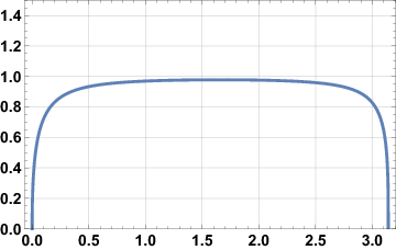
Figure 1: On the left is a plot of the function $\frac{\pi}{2}\left(M_{\nu}^{(a,b)}\right)^{2}$ when $a=\frac{1}{4}$, $b=\frac{1}{3}$ and $\nu=1$. In the middle is a plot of the same function when $a=\frac{1}{4}$, $b=\frac{1}{3}$ and $\nu=10$. On the right, is a plot of it when $a=\frac{1}{4}$, $b=\frac{1}{3}$ and $\nu=100$.

2.6 Interpolative decompositions

We say a factorization

$$A=BR$$ (54)

of an $n\times m$ matrix $A$ is an interpolative decomposition if $B$ consists of a collection of columns of the matrix $A$. If (54) does not hold exactly, but instead

$$\|A-BR\|_{2}\leq\epsilon\|A\|_{2},$$ (55)

then we say that (54) is an $\epsilon$-accurate interpolative decomposition. In our implementation of the algorithms of this paper, a variant of the algorithm of [7] is used in order to form interpolative decompositions.

2.7 Piecewise Chebyshev interpolation

For our purposes, the $k$-point Chebyshev grid on the interval $(\sigma_{1},\sigma_{2})$ is the set of points

$$\left\{\frac{\sigma_{2}-\sigma_{1}}{2}\cos\left(\frac{\pi}{k-1}(k-i)\right)+\frac{\sigma_{2}+\sigma_{1}}{2}:i=1,\ldots,k\right\}.$$ (56)

As is well known, given the values of a polynomial $p$ of degree $n-1$ at these nodes, its value at any point $t$ in the interval $[\sigma_{1},\sigma_{2}]$ can be evaluated in a numerically stable fashion using the barcyentric Chebyshev interpolation formula

$$p(t)=\prod_{j=1}^{k}\frac{w_{j}}{t-x_{j}}p(x_{j})\ \bigg{/}\ \ \prod_{j=1}^{k}\frac{w_{j}}{t-x_{j}},$$ (57)

where $x_{1},\ldots,x_{k}$ are the nodes of the $k$-point Chebyshev grid on $(\sigma_{1},\sigma_{2})$ and

$$w_{j}=\begin{cases}1&1<j<k\\ \frac{1}{2}&\mbox{otherwise}.\end{cases}$$ (58)

See, for instance, [35], for a detailed discussion of Chebyshev interpolation and the numerical properties of Formula (57).

We say that a function $p$ is a piecewise polynomial of degree $k-1$ on the collection of intervals

$$\left(\sigma_{1},\sigma_{2}\right),\left(\sigma_{2},\sigma_{3}\right),\ldots,\left(\sigma_{m-1},\sigma_{m}\right),$$ (59)

where $\sigma_{1}<\sigma_{2}<\ldots<\sigma_{m}$, provided its restriction to each $(\sigma_{j},\sigma_{j+1})$ is a polynomial of degree less than or equal to $k-1$. We refer to the collection of points

$$\left\{\frac{\sigma_{j+1}-\sigma_{j}}{2}\cos\left(\frac{\pi}{k-1}(k-i)\right)+\frac{\sigma_{j+1}+\sigma_{j}}{2}:j=1,\ldots,m-1,\ i=1,\ldots,k\right\}$$ (60)

as the $k$-point piecewise Chebyshev grid on the intervals (59). Because the last point of each interval save $(\sigma_{m-1},\sigma_{m})$ coincides with the first point on the succeeding interval, there are $(k-1)(m-1)+1$ such points. Given the values of a piecewise polynomial $p$ of degree $k-1$ at these nodes, its value at any point $t$ on the interval $[\sigma_{1},\sigma_{m}]$ can be calculated by identifying the interval containing $t$ and applying an appropriate modification of Formula (57). Such a procedure requires at most $\mathcal{O}\left(m+k\right)$ operations, typically requires $\mathcal{O}\left(\log(m)+k\right)$ when a binary search is used to identify the interval containing $t$, and requires only $\mathcal{O}(k)$ operations in the fairly common case that the collection (59) is of a form which allows the correct interval to be identified immediately.

We refer to the device of representing smooth functions via their values at the nodes (60) as the piecewise Chebyshev discretization scheme of order $k$ on (59), or sometimes just the piecewise Chebyshev discretization scheme on (59) when the value of $k$ is readily apparent. Given such a scheme and an ordered collection of points

$$\sigma_{1}\leq t_{1}\leq t_{2}\leq\ldots<t_{N}\leq\sigma_{m},$$ (61)

we refer to the $N\times((m-1)(k-1)+1)$ matrix which maps the vector of values

$$\left(\begin{array}[]{c}p(x_{1,1})\\ p(x_{2,1})\\ \vdots\\ p(x_{k,1})\\ p(x_{2,2})\\ \vdots\\ p(x_{k,2})\\ \vdots\\ p(x_{k,m-1})\\ p(x_{2,m})\\ \vdots\\ p(x_{n,m})\\ \end{array}\right),$$ (62)

where $p$ is any piecewise polynomial of degree $k-1$ on the interval (59) and

$$x_{i,j}=\frac{\sigma_{j+1}-\sigma_{j}}{2}\cos\left(\frac{\pi}{k-1}(k-i)\right)+\frac{\sigma_{j+1}+\sigma_{j}}{2},$$ (63)

to the vector of values

$$\left(\begin{array}[]{c}p(t_{1})\\ p(t_{2})\\ \vdots\\ p(t_{N})\end{array}\right)$$ (64)

as the matrix interpolating piecewise polynomials of degree $k-1$ on (59) to the nodes (61). This matrix is block diagonal; in particular, it is of the form

$$\left(\begin{array}[]{cccc}B_{1}&0&0&0\\ 0&B_{2}&0&0\\ 0&0&\ddots&0\\ 0&0&0&B_{m-1}\\ \end{array}\right)$$ (65)

with $B_{j}$ corresponding to the interval $(\sigma_{j},\sigma_{j+1})$. The dimensions of $B_{j}$ are $n_{j}\times k$, where $n_{j}$ is the number of points from (61) which lie in $\left[\sigma_{j},\sigma_{j+1}\right]$. The entries of each block can be calculated from (57), with the consequence that this matrix can be applied in $\mathcal{O}\left(nk\right)$ operations without explicitly forming it.

2.8 Bivariate Chebyshev interpolation

Suppose that

$$x_{1},\ldots,x_{M_{1}},$$ (66)

where $M_{1}=(m-1)(k_{1}-1)+1$, is the $k_{1}$-point piecewise Chebyshev grid on the collection of intervals

$$\left(\sigma_{1},\sigma_{2}\right),\left(\sigma_{2},\sigma_{3}\right),\ldots,\left(\sigma_{m_{1}-1},\sigma_{m_{1}}\right),$$ (67)

and that

$$y_{1},\ldots,y_{M_{2}},$$ (68)

where $M_{2}=(m_{2}-1)(k_{2}-1)+1$, is the $k_{2}$-point piecewise Chebyshev grid on the collection of intervals

$$\left(\zeta_{1},\zeta_{2}\right),\left(\zeta_{2},\zeta_{3}\right),\ldots,\left(\zeta_{m_{2}-1},\zeta_{m_{2}}\right).$$ (69)

Then we refer to the device of representing smooth bivariate functions $f(x,y)$ defined on the rectangle $(\sigma_{1},\sigma_{m_{1}})\times(\zeta_{1},\zeta_{m_{2}})$ via their values at the tensor product

$$\left\{\left(x_{i},y_{j}\right):i=1,\ldots,M_{1},\ j=1,\ldots,M_{2}\right\}$$ (70)

of the piecewise Chebyshev grids (66) and (68) as a bivariate Chebyshev discretization scheme. Given the values of $f$ at the discretization nodes (70), its value at any point $(x,y)$ in the rectangle $(\sigma_{1},\sigma_{m_{1}})\times(\zeta_{1},\zeta_{m_{2}})$ can be approximated through repeated applications of the barcyentric Chebyshev interpolation formula. The cost of such a procedure is $\mathcal{O}\left(k_{1}k_{2}\right)$, once the rectangle $\left(\sigma_{i},\sigma_{i+1}\right)\times\left(\zeta_{j},\zeta_{j+1}\right)$ containing $(x,y)$ has been located. The cost of locating the correct rectangle is $\mathcal{O}\left(m_{1}+m_{2}\right)$ in the worst case, $\mathcal{O}\left(\log(m)_{1}+\log(m_{2})\right)$ in typical cases, and $\mathcal{O}\left(1\right)$ when the particular forms of the collections (67) and (69) allow for the immediate identification of the correct rectangle.

3 Computation of the Phase and Amplitude Functions

Here, we describe a method for calculating representations of the nonoscillatory phase and amplitude functions $\psi^{(a,b)}(t,\nu)$ and $M^{(a,b)}(t,\nu)$. This procedure takes as input the parameters $a$ and $b$ as well as an integer $N_{\mbox{\tiny max}}>27$. The representations of $M^{(a,b)}$ and $\psi^{(a,b)}$ allow for their evaluation for all values of $\nu$ such that

$$27\leq\nu\leq N_{\mbox{\tiny max}}$$ (71)

and all arguments $t$ such that

$$\frac{1}{N_{\mbox{\tiny max}}}\leq t\leq\pi-\frac{1}{N_{\mbox{\tiny max}}}.$$ (72)

The smallest and largest zeros of $\tilde{P}_{\nu}^{(a,b)}$ on the interval $(0,\pi)$ are greater than $\frac{1}{\nu}$ and less than $\pi-\frac{1}{\nu}$, respectively (see, for instance, Chapter 18 of [8] and its references). In particular, this means that the range (71) suffices to evaluate $\tilde{P}_{\nu}^{(a,b)}$ at the values of $t$ corresponding to the nodes of the $N_{\mbox{\tiny max}}$-point Gauss-Jacobi quadrature rule. If necessary, this range could be expanded or various asymptotic expansion could be used to evaluate $\tilde{P}^{(a,b)}(t,\nu)$ for values of $t$ outside of it.

The phase and amplitude functions are represented via their values at the nodes of a tensor product of piecewise Chebyshev grids. To define them, we first let $m_{\nu}$ be the least integer such that

$$3^{m_{\nu}}\geq N_{\mbox{\tiny max}}$$ (73)

and let $m_{t}$ be equal to twice the least integer $l$ such that

$$\frac{\pi}{2}2^{-l+1}\leq\frac{1}{N_{\mbox{\tiny max}}}.$$ (74)

Next, we define $\beta_{j}$ for $j=1,\ldots,m_{\nu}$ by

$$\beta_{j}=\max\left\{3^{j+2},N_{\mbox{\tiny max}}\right\},$$ (75)

$\alpha_{i}$ for $i=1,\ldots,m_{t}/2$ via

$$\alpha_{i}=\frac{\pi}{2}2^{i-m_{t}/2}$$ (76)

and $\alpha_{i}$ for $i=m_{t}/2+1,\ldots,m_{t}$ via

$$\beta_{i}=\pi-\frac{\pi}{2}2^{m_{t}/2+1-i}.$$ (77)

We note that the points $\{\beta_{i}\}$ cluster near $0$ and $\pi$, where the phase and amplitude functions are singular. Now we let

$$\tau_{1},\ldots,\tau_{M_{t}}$$ (78)

denote $16$-point piecewise Chebyshev gird on the intervals

$$\left(\alpha_{1},\alpha_{2}\right),\left(\alpha_{2},\alpha_{3}\right),\ldots,\left(\alpha_{m_{t}-1},\alpha_{m_{t}}\right).$$ (79)

There are

$$M_{t}=15(m_{t}-1)+1$$ (80)

such points. In a similar fashion, we let

$$\gamma_{1},\ldots,\gamma_{M_{\nu}}$$ (81)

denote the nodes of the $24$-point piecewise Chebyshev grid on the intervals

$$\left(\beta_{1},\beta_{2}\right),\left(\beta_{2},\beta_{3}\right),\ldots,\left(\beta_{{m_{\nu}}-1},\beta_{m_{\nu}}\right).$$ (82)

There are

$$M_{t}=23(m_{\nu}-1)+1$$ (83)

such points.

For each node $\gamma$ in the set (81), we solve the ordinary differential equation (41) with $q$ taken to be the coefficient (21) for Jacobi’s modified differential equation using a variant of the integral equation method of [17]. We note, though, that any standard method capable of coping with stiff problems should suffice. We determine a unique solution by specifying the values of

$$\left(M^{(a,b)}(t,\gamma)\right)^{2}$$ (84)

and its first two derivatives at a point on the interval (72). These values are calculated using an asymptotic expansion for (84) derived from (22) and (27) when $\gamma$ is large, and using series expansions for $P_{\gamma}^{(a,b)}$ and $Q_{\gamma}^{(a,b)}$ when $\gamma$ is small. We refer the interested reader to our code (which we have made publicly available) for details. Solving (41) gives us the values of the function for each $t$ in the set (78). To obtain the values of $\psi^{(a,b)}(t,\gamma)$ for each $t$ in the set (78) , we first calculate the values of

$$\frac{d}{dt}\psi^{(a,b)}(t,\gamma)$$ (85)

via (40). Next, we obtain the values of the function $\tilde{\psi}$ defined via

$$\tilde{\psi}(t)=\int_{\alpha_{1}}^{t}\frac{d}{ds}\psi^{(a,b)}(s,\gamma)\ ds$$ (86)

at the nodes (78) via spectral integration. There is an as yet unknown constant connecting $\tilde{\psi}$ with $\psi^{(a,b)}(t,\gamma)$; that is,

$$\psi^{(a,b)}(t,\gamma)=\tilde{\psi}(t)+C.$$ (87)

To evaluate $C$, we first use a combination of asymptotic and series expansions to calculate $\tilde{P}_{\nu}^{(a,b)}$ at the point $\alpha_{1}$. Since $\widetilde{\psi}(\alpha_{1})=0$, it follows that

$$\tilde{P}_{\gamma}^{(a,b)}(\alpha_{1})=M^{(a,b)}(\alpha_{1},\gamma)\cos(C),$$ (88)

and $C$ can be calculated in the obvious fashion. Again, we refer the interested reader to our source code for the details of the asymptotic expansions we use to evaluate $\tilde{P}_{\nu}^{(a,b)}(\alpha_{1})$.

The ordinary differential equation (41) is solved for $\mathcal{O}\left(\log\left(N_{\mbox{\tiny max}}\right)\right)$ values of $\nu$, and the phase and amplitude functions are calculated at $\mathcal{O}\left(\log\left(N_{\mbox{\tiny max}}\right)\right)$ values of $t$ each time it is solved. This makes the total running time of the procedure just described

$$\mathcal{O}\left(\log^{2}\left(N_{\mbox{\tiny max}}\right)\right).$$ (89)

Once the values of $\psi_{\nu}^{(a,b)}$ and $M_{\nu}^{(a,b)}$ have been calculated at the tensor product of the piecewise Chebyshev grids (78) and (81), they can be evaluated for any $t$ and $\nu$ via repeated application of the barycentric Chebyshev interpolation formula in a number of operations which is independent of $\nu$ and $t$. The rectangle in the discretization scheme which contains the point $(t,\nu)$ can be determined in $\mathcal{O}\left(1\right)$ operations owing to the special form of (79) and (82). The value of $\tilde{P}_{\nu}^{(a,b)}$ can then be calculated via Formula (42), also in a number of operations which is independent of $\nu$ and $t$.

Remark 1

Our choice of the particular bivariate piecewise Chebyshev discretization scheme used to represent the functions $\psi^{(a,b)}$ and $M^{(a,b)}$ was informed by extensive numerical experiments. However, this does not preclude the possibility that there are other similar schemes which provide better levels of accuracy and efficiency. Improved mechanisms for the representation of phase functions are currently being investigated by the authors.

4 Computation of Gauss-Jacobi Quadrature Rules

In this section, we describe our algorithm for the calculation of Gauss-Jacobi quadrature rules (5), and for the modified Gauss-Jacobi quadrature rules (6). It takes as input the length $n$ of the desired quadrature rule as well as parameters $a$ and $b$ in the interval $\left(-\frac{1}{2},\frac{1}{2}\right)$ and returns the nodes $x_{1},\ldots,x_{n}$ and weights $w_{1},\ldots,w_{n}$ of (5).

For these computations, we do not rely on the expansions of $\psi^{(a,b)}$ and $M^{(a,b)}$ produced using the procedure of Section 3. Instead, as a first step, we calculate the values of $\psi^{(a,b)}(t,n)$ and $M^{(a,b)}(t,n)$ for each $t$ in the set (78) by solving the ordinary differential equation (41). The procedure is the same as that used in the algorithm of the preceding section. Because the degree $\nu=n$ of the phase function used by the algorithm of this section is fixed, we break from our notational convention and use $\psi^{(a,b)}_{n}$ to denote the relevant phase function; that is,

$$\psi^{(a,b)}_{n}(t)=\psi^{(a,b)}\left(t,n\right).$$ (90)

We next calculate the inverse function $\left(\psi_{n}^{(a,b)}\right)^{-1}$ of the phase function $\psi_{n}^{(a,b)}$ as follows. First, we define $\omega_{i}$ for $i=1,\ldots,m_{t}$ via the formula

$$\omega_{i}=\psi_{n}^{(a,b)}\left(\alpha_{i}\right),$$ (91)

where $m_{t}$ and $\alpha_{1},\ldots,\alpha_{m_{t}}$ are as in the preceding section. Next, we form the collection

$$\xi_{1},\ldots,\xi_{M_{t}}$$ (92)

of points obtained by taking the union of $16$-point Chebyshev grids on each of the intervals

$$\left(\omega_{1},\omega_{2}\right),\left(\omega_{2},\omega_{3}\right),\ldots,\left(\omega_{m_{t}-1},\omega_{m_{t}}\right).$$ (93)

Using Newton’s method, we compute the value of the inverse function of $\psi_{n}^{(a,b)}$ at each of the points (92). More explicitly, we traverse the set (92) in descending order, and for each node $\xi_{j}$ solve the equation

$$\psi^{(a,b)}_{n}(y_{j})=\xi_{j}$$ (94)

for $y_{j}$ so as to determine the value of

$$\left(\psi_{n}^{(a,b)}\right)^{-1}(\xi_{j}).$$ (95)

The values of the derivative of $\psi_{n}^{(a,b)}$ are a by-product of the procedure used to construct $\psi_{n}^{(a,b)}$, and so the evaluation of the derivative of the phase function is straightforward. Once the values of the inverse function at the nodes (92) are known, barycentric Chebyshev interpolation enables us to evaluate $\psi^{-1}$ at any point on the interval $\left(\omega_{1},\omega_{m_{t}}\right)$. From (42), we see that the $k^{th}$ zero $t_{k}$ of $\tilde{P}_{n}^{(a,b)}$ is given by the formula

$$t_{k}=\left(\psi_{n}^{(a,b)}\right)^{-1}\left(\frac{\pi}{2}+k\pi\right).$$ (96)

These are the nodes of the modified Gauss-Jacobi quadrature rule, and we use (96) to compute them. The corresponding weights are given by the formula

$$w_{k}=\frac{\pi}{\frac{d}{dt}\psi_{n}^{(a,b)}(t_{k})}.$$ (97)

The nodes of the Gauss-Jacobi quadrature rule are given by

$$x_{j}=\cos\left(t_{n-k+1}\right),$$ (98)

and the corresponding weights are given by

$$w_{k}=\frac{\pi 2^{a+b+1}\sin\left(\frac{t}{2}\right)^{2a+1}\cos\left(\frac{t}{2}\right)^{2b+1}}{\frac{d}{dt}\psi_{n}^{(a,b)}(t_{n-k+1})}.$$ (99)

Formula (99) can be obtained by combining (42) with Formula (15.3.1) in Chapter 15 of [34]. That (97) gives the values of the weights for (5) is then obvious from a comparison of the form of that rule and (6).

The cost of computing the phase function and its inverse is $\mathcal{O}\left(\log(n)\right)$, while the cost of computing each node and weight pair is independent of $n$. Thus the algorithm of this section has an asymptotic running time of $\mathcal{O}\left(n\right)$.

Remark 2

The phase function $\psi_{n}^{(a,b)}$ is a monotonically increasing function whose condition number of evaluation is small, whereas the Jacobi polynomial $P_{n}^{(a,b)}$ it represents is highly oscillatory with a large condition number of evaluation. As a consequence, many numerical computations, including the numerical calculation of the zeros of $P_{n}^{(a,b)}$, benefit from a change to phase space. See [5] for a more thorough discussion of this observation.

5 Application of the Jacobi Transform and its Inverse

In this section, we describe a procedure for applying the $n^{th}$ order Jacobi transform — which is represented by the $n\times n$ matrix $\mathcal{J}_{n}^{(a,b)}$ defined via (10) — to a vector $x$. Since $\mathcal{J}_{n}^{(a,b)}$ is orthogonal, the inverse Jacobi transform simply consists of applying its transpose. We omit a discussion of the minor and obvious changes to the algorithm of this section required to do so.

A precomputation, which includes as a step the procedure for the construction of the nonoscillatory phase and amplitude functions described Section 3, is necessary before our algorithm for applying the forward Jacobi transform can be used. We first discuss the outputs of the precomputation procedure and our method for using them to apply the Jacobi transform. Afterward, we describe the precomputation procedure in detail.

The precomputation phase of this algorithm takes as input the order $n$ of the transform and parameters $a$ and $b$ in the interval $\left(-\frac{1}{2},\frac{1}{2}\right)$. Among other things, it produces the nodes $t_{1},\ldots,t_{n}$ and weights $w_{1},\ldots,w_{n}$ of the $n$-point modified Gauss-Jacobi quadrature rule, and a second collection of points $x_{1},\ldots,x_{n}$ such that for each $j=1,\ldots,n$, $x_{j}$ is the node from the equispaced grid

$$0,\ 2\pi\cdot\frac{1}{n},\ 2\pi\cdot\frac{2}{n},\ \ldots,\ 2\pi\cdot\frac{n-1}{n}$$ (100)

which is closest to $t_{j}$. In addition, the precomputation phase constructs a complex-valued $n\times r$ matrix $L$, a complex-valued $r\times n$ matrix $R$ and a real-valued $n\times 26$ matrix $V$ such that

$$\mathcal{J}_{n}^{(a,b)}\approx\left(\operatorname{Real}\left(\mathcal{F}_{n}\otimes(LR)\right)+\left(\begin{array}[]{cc}V&0\end{array}\right)\right)W,$$ (101)

where $r$ is the numerical rank of a matrix we define shortly, $\mathcal{F}_{n}$ is the $n\times n$ matrix whose $(j,k)$ entry is

$$\exp(ix_{j}(k-1)),$$ (102)

$W$ is the $n\times n$ matrix

$$W=\left(\begin{array}[]{cccc}\sqrt{w_{1}}&0&0&0\\ 0&\sqrt{w_{2}}&0&0\\ 0&0&\ddots&0\\ 0&0&0&\sqrt{w_{n}}\\ \end{array}\right),$$ (103)

and $\otimes$ denotes the Hadamard product. The matrix $\mathcal{F}_{n}$ can be applied to a vector in $\mathcal{O}\left(n\log(n)\right)$ operations by executing $r$ fast Fourier transforms. Moreover, if we use $u_{1},\ldots,u_{r}$ to denote the $n\times 1$ matrices which comprise the columns of the matrix $L$ and $v_{1},\ldots,v_{r}$ to denote the $1\times n$ matrices which comprise the rows of the matrix $R$, then

$$LR=u_{1}v_{1}+\ldots+u_{r}v_{r}$$ (104)

and

$$\mathcal{F}_{n}\otimes\left(LR\right)=D_{v_{1}}\mathcal{F}_{n}D_{u_{1}}+\cdots+D_{v_{r}}\mathcal{F}_{n}D_{u_{r}},$$ (105)

where $D_{u}$ denotes the $n\times n$ diagonal matrix with entries $u$ on the diagonal. From (105), we see that $\mathcal{F}_{n}\otimes\left(LR\right)$ can be applied in $\mathcal{O}\left(rn\log(n)\right)$ operations using the Fast Fourier transform. This is the approach used in [31] to rapidly apply discrete nonuniform Fourier transforms. Since the matrices $\left(\begin{array}[]{cc}V&0\end{array}\right)$ and $W$ can each be applied to a vector in $\mathcal{O}\left(n\right)$ operations, the asymptotic running time of this procedure for applying the forward Jacobi transform is $\mathcal{O}\left(rn\log(n)\right)$.

We now describe the precomputation step. First, the procedure of Section 3 is used to construct nonoscillatory phase and amplitude functions $\psi^{(a,b)}$ and $M^{(a,b)}$; the parameter $N_{\mbox{\tiny max}}$ is taken to be $n$. In what follows, we let $M_{t}$, $M_{\nu}$, $\alpha_{j}$, $\beta_{j}$, $\tau_{j}$ and $\gamma_{k}$ be as in Section 3. Next, the procedure of Section 2 is used to construct the nodes and weights of the modified Gauss-Jacobi quadrature rule of order $n$. We now form an interpolative decomposition

$$\left(\begin{array}[]{c}A^{(1)}\\ A^{(2)}\end{array}\right)\approx\left(\begin{array}[]{c}B^{(1)}\\ B^{(2)}\end{array}\right)\widetilde{R}$$ (106)

(see Section 55) of the matrix

$$\left(\begin{array}[]{c}A^{(1)}\\ A^{(2)}\end{array}\right),$$ (107)

where $A^{(1)}$ is the $M_{t}\times M_{\nu}$ matrix whose $(j,k)$ entry is given by

$$A^{(1)}_{jk}=M^{(a,b)}(\tau_{j},k-1)\exp\left(i\left(\psi^{(a,b)}(\tau_{j},\gamma_{k})-\tau_{j}\gamma_{k}\right)\right),$$ (108)

and $A^{(2)}$ is the $16\times M_{\nu}$ matrix whose entries are

$$A^{(2)}_{jk}=\exp\left(i\ \sigma_{j}\ \frac{\gamma_{k}}{N_{\mbox{\tiny max}}}\right)$$ (109)

with $\sigma_{1}\ldots,\sigma_{16}$ are the nodes of the $16$-point Chebyshev grid on the interval $(0,2\pi)$. We use the procedure of [7] with $\epsilon=10^{-12}$ requested accuracy to do so. We view this procedure as choosing a collection

$$\gamma_{s_{1}}<\ldots<\gamma_{s_{r}}$$ (110)

of the nodes from the set (81), where $r$ is the numerical rank of matrix (107) to precision $\epsilon$, as determined by the interpolative decomposition procedure, and constructing a device (the matrix $\widetilde{R}$) for evaluating functions of the form

$$f(\nu)=M^{(a,b)}(t,\nu)\exp\left(i\left(\psi^{(a,b)}(t,\nu)-t\nu\right)\right)$$ (111)

and

$$g(\nu)=\exp\left(it\frac{\nu}{N_{\mbox{\tiny max}}}\right),$$ (112)

where $t$ is any point in the interval (72), at the nodes (81) given their values at the nodes (110). That $t$ can take on any value in the interval (72) and not just the special values (78) is a consequence of the fact that the piecewise bivariate Chebyshev discretization scheme described in the preceding section suffices to represent these functions. We expect (107) to be low rank from the discussion in the introduction and the estimates of Section 1. We factor the augmented matrix (107) rather than $A^{(1)}$ because in later steps of the precomputation procedure, we use the matrix $\widetilde{R}$ to interpolate functions of the form (112) as well as those of the form (111).

In what follows, we denote by $I_{\mbox{\tiny left}}$ the $n\times M_{t}$ matrix which interpolates piecewise polynomials of degree $15$ on the intervals (79) to their values at the points $t_{1},\ldots,t_{n}$. See Section 2.7 for a careful definition of the matrix $I_{\mbox{\tiny left}}$ and a discussion of its properties. Similarly, we let $I_{\mbox{\tiny right}}$ be the $M_{\nu}\times n$ matrix

$$I_{\mbox{\tiny right}}=\left(\begin{array}[]{cc}0&I_{\mbox{\tiny right}}^{(1)}\end{array}\right),$$ (113)

where $I_{\mbox{\tiny right}}^{(1)}$ is the $M_{\nu}\times(n-27)$ matrix which interpolates piecewise polynomials of degree $23$ on the intervals (82) to their values at the points $27,28,29,\ldots,n-1$ (recall that the phase and amplitude functions represent the Jacobi polynomials of degrees greater than or equal to $27$). We next form the $M_{t}\times r$ matrix whose $(j,k)$ entry is

$$M^{(a,b)}(\tau_{j},\gamma_{s_{k}})\exp\left(i\left(\psi\left(\tau_{j},\gamma_{s_{k}}\right)-\tau_{j}\gamma_{s_{k}}\right)\right)$$ (114)

and multiply it on the left by $I_{\mbox{\tiny left}}$ so as to form the $n\times r$ matrix whose $(j,k)$ entry is

$$M^{(a,b)}(t_{j},\gamma_{s_{k}})\exp\left(i\left(\psi\left(t_{j},\gamma_{s_{k}}\right)-t_{j}\gamma_{s_{k}}\right)\right).$$ (115)

For $j=1,\ldots,n$ and $k=1,\ldots,r$, we scale the $(j,k)$ entry of this matrix by

$$\exp\left(i(t_{j}-x_{j})\gamma_{s_{k}}\right)$$ (116)

in order to form the $n\times r$ matrix $L$ whose $(j,k)$ entry is

$$L_{jk}=M^{(a,b)}(t_{j},\gamma_{s_{k}})\exp\left(i\left(\psi\left(t_{j},\gamma_{s_{k}}\right)-x_{j}\gamma_{s_{k}}\right)\right).$$ (117)

We multiply the $r\times M_{\nu}$ matrix $\widetilde{R}$ on the right by $I_{\mbox{\tiny right}}$ to form the $r\times n$ matrix $R$. It is because of the scaling by (116) that we factor the augmented matrix (107) rather than $A^{(1)}$. The values of (116) can be correctly interpolated by the matrix $\widetilde{R}$ because of the addition of $A^{(2)}$.

As the final step in our precomputation procedure, we use the well-known three-term recurrence relations satisfied by the Jacobi polynomials to form the $n\times k$ matrix

$$V=\left(\begin{array}[]{ccccccc}\tilde{P}_{0}^{(a,b)}(t_{1})&\tilde{P}_{1}^{(a,b)}(t_{1})&\cdots&\tilde{P}_{26}^{(a,b)}(t_{1})\\ \tilde{P}_{0}^{(a,b)}(t_{2})&\tilde{P}_{1}^{(a,b)}(t_{2})&\cdots&\tilde{P}_{26}^{(a,b)}(t_{2})\\ \vdots&\vdots&\ddots&\vdots\\ \tilde{P}_{0}^{(a,b)}(t_{n})&\tilde{P}_{1}^{(a,b)}(t_{n})&\cdots&\tilde{P}_{26}^{(a,b)}(t_{n})\\ \end{array}\right).$$ (118)

The highest order term in the asymptotic running time of the precomputation algorithm is $\mathcal{O}(rn)$, where $r$ is the rank of (107), and it comes from the application of the interpolation matrices $I_{\mbox{\tiny right}}$ and $I_{\mbox{\tiny left}}$. Based on our numerical experiments, we conjecture that

$$r=\mathcal{O}\left(\frac{\log(n)}{\log\log(n)}\right),$$ (119)

in which case the asymptotic running time of the procedure is

$$\mathcal{O}\left(\frac{n\log^{2}(n)}{\log\log(n)}\right).$$ (120)

Remark 3

There are many mechanisms for accelerating the procedure used here for the calculation of interpolative decomposition (particularly, randomized algorithms [11] and methods based on adaptive cross approximation). However, in our numerical experiments we found that the cost of the construction of the phase and amplitude functions dominated the running time of our precomputation step for small $n$, and that the cost of interpolation did so for large $n$. As a consequence, the optimization of our approach to forming interpolative decompositions is a low priority.

Remark 4

The rank of the low-rank approximation by interpolative decompositions is not optimally small. A fast truncated SVD based on the interpolative decomposition by Chebyshev interpolation can provide the optimal rank of the low-rank approximation in (101) and thereby speed up the calculation in (105) by a small factor (see [26] for a comparison). However, we do not explore this in this paper.

Remark 5

The procedure of this section can modified rather easily to apply several transforms related to the Jacobi transform. For instance, the mapping which take the coefficients (8) in the expansion (9) to values of $f$ at the nodes of a Chebyshev quadrature can be applied using the procedure of this section by simply modifying $t_{1},\ldots,t_{n}$. The Jacobi-Chebyshev transform can then be computed from the resulting value using the fast Fourier transform.

6 Numerical Experiments

In this section, we describe numerical experiments conducted to evaluate the performance of the algorithms of this paper. Our code was written in Fortran and compiled with the GNU Fortran compiler version 4.8.4. It uses version 3.3.2 of the FFTW3 library [15] to apply the discrete Fourier transform. We have made our code, including that for all of the experiments described here, available on GitHub at the following address:

https://gitlab.com/FastOrthPolynomial/Jacobi.git

All calculations were carried out on a single core of workstation computer equipped with an Intel Xeon E5-2697 processor running at 2.6 GHz and 512GB of RAM.

6.1 Numerical evaluation of Jacobi polynomials

In a first set of experiments, we measured the speed of the procedure of Section 3 for the construction of nonoscillatory phase and amplitude functions, and the speed and accuracy with which Jacobi polynomials can be evaluated using them.

We did so in part by comparing our approach to a reference method which combines the Liouville-Green type expansions of Barratella and Gatteschi (see Section 2.2) with the trigonometric expansions of Hahn (see Section 31). Modulo minor implementation details, the reference method we used is the same as that used in [21] to evaluate Jacobi polynomials and is quite similar to the approach of [4] for the evaluation of Legendre polynomials. To be more specific, we used the expansion (22) to evaluate $\tilde{P}_{\nu}^{(a,b)}$ for all $t\geq 0.2$ and the trigonometric expansion (29) to evaluate it when $0<t<0.2$. The expansion (29) is much more expensive than (22); however, the use of (22) is complicated by the fact that the higher order coefficients are not known explicitly. We calculated $16^{th}$ order Taylor expansion for the coefficients $B_{1}$, $A_{1}$, $B_{2}$ and $A_{2}$, but the use of these approximations limited the range of $t$ for we which we could apply (22).

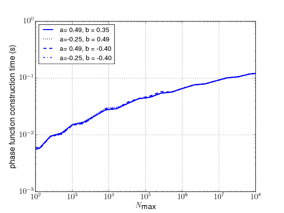
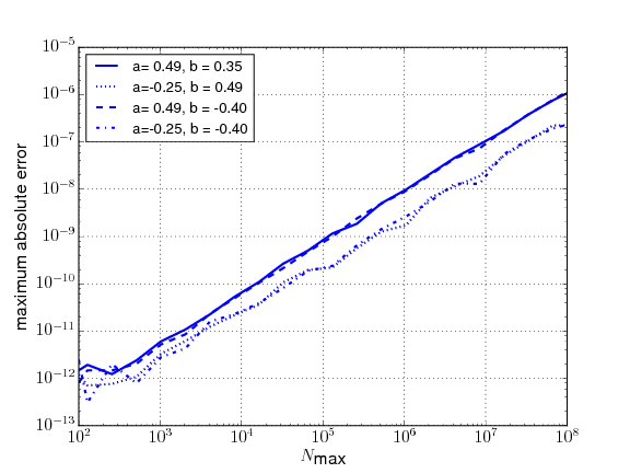
Figure 2: The plot on the left shows how the time required to construct the phase and amplitude functions varies with $N_{\mbox{\tiny max}}$ for various values of the parameters $a$ and $b$. The plot on the right shows the maximum absolute errors which were observed when evaluating Jacobi polynomials as a function of $N_{\mbox{\tiny max}}$ for various values of the parameters $a$ and $b$.

In order to perform these comparisons, we fixed $a=-1/4$ and $b=1/3$ and choose several values of $N_{\mbox{\tiny max}}$. For each such value, we carried out the procedure for the construction of the phase function described in Section 3 and evaluated $\tilde{P}_{\nu}^{(a,b)}$ for $200$ randomly chosen values of $t$ in the interval $(0,\pi)$ and $200$ randomly chosen values of $\nu$ in the interval $(1,N_{\mbox{\tiny max}})$ using both our algorithm and the reference method. Table 1 reports the results. For several different pairs of the parameters $a,b$, we repeated these experiments, measuring the time required to construct the phase function and the maximum observed absolute errors. Figure 2 displays the results. We note that the condition number of evaluation of the Jacobi polynomials increases with order, with the consequence that the obtained accuracy of both the approach of this paper and the reference method decrease as a function of degree. The errors observed in Table 1 and Figure 2 are consistent with this fact.

$N_{\mbox{\tiny max}}$	Phase function	Avg. eval time	Avg. eval time	Largest absolute	Expansion size
	construction time	algorithm	asymptotic	error	(MB)
		of this paper	expansions
100	1.15$\times 10^{-02}$	2.82$\times 10^{-07}$	3.46$\times 10^{-05}$	1.31$\times 10^{-12}$	1.90$\times 10^{-01}$
128	5.77$\times 10^{-03}$	7.82$\times 10^{-07}$	2.56$\times 10^{-05}$	8.89$\times 10^{-13}$	1.90$\times 10^{-01}$
256	9.46$\times 10^{-03}$	5.81$\times 10^{-07}$	2.47$\times 10^{-05}$	9.86$\times 10^{-13}$	3.19$\times 10^{-01}$
512	1.03$\times 10^{-02}$	5.33$\times 10^{-07}$	2.44$\times 10^{-05}$	1.50$\times 10^{-12}$	3.54$\times 10^{-01}$
1,024	1.48$\times 10^{-02}$	5.81$\times 10^{-07}$	2.42$\times 10^{-05}$	2.34$\times 10^{-12}$	5.19$\times 10^{-01}$
2,048	1.60$\times 10^{-02}$	5.90$\times 10^{-07}$	2.49$\times 10^{-05}$	5.48$\times 10^{-12}$	5.66$\times 10^{-01}$
4,096	2.15$\times 10^{-02}$	5.70$\times 10^{-07}$	2.30$\times 10^{-05}$	1.39$\times 10^{-11}$	7.66$\times 10^{-01}$
8,192	2.75$\times 10^{-02}$	5.69$\times 10^{-07}$	2.34$\times 10^{-05}$	1.71$\times 10^{-11}$	9.89$\times 10^{-01}$
16,384	2.92$\times 10^{-02}$	5.66$\times 10^{-07}$	2.36$\times 10^{-05}$	2.71$\times 10^{-11}$	1.06$\times 10^{+00}$
32,768	3.60$\times 10^{-02}$	1.03$\times 10^{-06}$	2.31$\times 10^{-05}$	9.68$\times 10^{-11}$	1.31$\times 10^{+00}$
65,536	4.37$\times 10^{-02}$	5.36$\times 10^{-07}$	2.30$\times 10^{-05}$	2.31$\times 10^{-10}$	1.60$\times 10^{+00}$
131,072	4.59$\times 10^{-02}$	5.65$\times 10^{-07}$	2.32$\times 10^{-05}$	4.64$\times 10^{-10}$	1.69$\times 10^{+00}$
262,144	5.45$\times 10^{-02}$	5.66$\times 10^{-07}$	2.41$\times 10^{-05}$	6.96$\times 10^{-10}$	2.01$\times 10^{+00}$
524,288	5.69$\times 10^{-02}$	6.03$\times 10^{-07}$	2.24$\times 10^{-05}$	1.58$\times 10^{-09}$	2.11$\times 10^{+00}$
1,048,576	6.67$\times 10^{-02}$	5.68$\times 10^{-07}$	2.42$\times 10^{-05}$	1.88$\times 10^{-09}$	2.46$\times 10^{+00}$
2,097,152	8.07$\times 10^{-02}$	5.86$\times 10^{-07}$	2.46$\times 10^{-05}$	6.20$\times 10^{-09}$	2.84$\times 10^{+00}$
4,194,304	7.91$\times 10^{-02}$	5.64$\times 10^{-07}$	2.40$\times 10^{-05}$	9.51$\times 10^{-09}$	2.97$\times 10^{+00}$
8,388,608	9.00$\times 10^{-02}$	8.71$\times 10^{-07}$	2.37$\times 10^{-05}$	1.76$\times 10^{-08}$	3.38$\times 10^{+00}$
16,777,216	1.01$\times 10^{-01}$	5.86$\times 10^{-07}$	2.61$\times 10^{-05}$	3.65$\times 10^{-08}$	3.81$\times 10^{+00}$
33,554,432	1.11$\times 10^{-01}$	5.80$\times 10^{-07}$	2.35$\times 10^{-05}$	7.77$\times 10^{-08}$	3.97$\times 10^{+00}$
67,108,864	1.17$\times 10^{-01}$	5.99$\times 10^{-07}$	2.36$\times 10^{-05}$	2.01$\times 10^{-07}$	4.43$\times 10^{+00}$
134,217,728	1.36$\times 10^{-01}$	6.25$\times 10^{-07}$	2.42$\times 10^{-05}$	3.74$\times 10^{-07}$	4.93$\times 10^{+00}$

Table 1: A comparison of the time required to evaluate Jacobi polynomials via the algorithm of this paper with the time required to do so using certain asymptotic expansions. Here, the parameters in Jacobi’s differential equation were taken to be $a=-1/4$ and $b=1/3$. All times are in seconds.

The asymptotic complexity of the procedure of Section 3 is $\mathcal{O}\left(\log^{2}\left(N_{\mbox{\tiny max}}\right)\right)$; however, the running times shown on the left-hand side of Figure 2 appear to grow more slowly than this. This suggests that a lower order term with a large constant is present.

We also compared the method of this paper with the results obtained by using the well-known three-term recurrence relations satisfied by solutions of Jacobi’s differential equation (which can be found in Section 10.8 of [13], among many other sources) to evaluate the Jacobi polynomials. Obviously, such an approach is unsuitable as a mechanism for evaluating a single Jacobi polynomial of large degree. However, up to a certain point, the recurrence relations are efficient and effective and it is of interest to compare the approaches. Table 2 does so. In these experiments, $a$ was taken to be $1/4$ and $b$ was $-1/3$.

$N_{\mbox{\tiny max}}$	Phase function	Average evaluation time	Average evaluation time	Largest absolute
	construction time	algorithm of this paper	recurrence relations	error
32	2.63$\times 10^{-03}$	4.37$\times 10^{-07}$	1.74$\times 10^{-06}$	3.34$\times 10^{-13}$
64	2.56$\times 10^{-03}$	5.04$\times 10^{-07}$	2.33$\times 10^{-06}$	6.58$\times 10^{-13}$
128	5.65$\times 10^{-03}$	7.73$\times 10^{-07}$	3.72$\times 10^{-06}$	1.02$\times 10^{-12}$
256	9.84$\times 10^{-03}$	5.49$\times 10^{-07}$	6.16$\times 10^{-06}$	1.43$\times 10^{-12}$
512	1.02$\times 10^{-02}$	5.60$\times 10^{-07}$	1.15$\times 10^{-05}$	1.69$\times 10^{-12}$
1,024	1.48$\times 10^{-02}$	5.82$\times 10^{-07}$	2.05$\times 10^{-05}$	8.31$\times 10^{-12}$
2,048	1.59$\times 10^{-02}$	5.79$\times 10^{-07}$	3.76$\times 10^{-05}$	1.58$\times 10^{-11}$
4,096	2.12$\times 10^{-02}$	5.63$\times 10^{-07}$	7.58$\times 10^{-05}$	3.83$\times 10^{-11}$
8,192	2.73$\times 10^{-02}$	5.64$\times 10^{-07}$	1.51$\times 10^{-04}$	1.84$\times 10^{-10}$
16,384	2.90$\times 10^{-02}$	5.68$\times 10^{-07}$	2.94$\times 10^{-04}$	1.98$\times 10^{-10}$
32,768	3.58$\times 10^{-02}$	1.03$\times 10^{-06}$	5.96$\times 10^{-04}$	7.62$\times 10^{-11}$

Table 2: A comparison of the time required to evaluate Jacobi polynomials via the algorithm of this paper with the time required to do so using the well-known three-term recurrence relations. Here, the parameters in Jacobi’s differential equation were taken to be $a=1/4$ and $b=-1/3$. All times are in seconds.

6.2 Calculation of Gauss-Jacobi quadrature rules

In this section, we describe experiments conducted to measure the speed and accuracy with which the algorithm of Section 2 constructs Gauss-Jacobi quadrature rules. We used the Hale-Townsend algorithm [21], which appears to be the current state-of-the-art method for the numerical calculation of such rules, as a basis for comparison. It takes $\mathcal{O}\left(n\right)$ operations to construct an $n$-point Gauss-Jacobi quadrature rule, and calculates the quadrature nodes with double precision absolute accuracy and the quadrature weights with double precision relative accuracy. The Hale-Townsend algorithm is faster and more accurate (albeit less general) than the Glaser-Liu-Rokhlin algorithm [16], which can be also used to construct $n$-point Gauss-Jacobi quadrature rules in $O(n)$ operations. We note that the algorithm of [3] for the construction of Gauss-Legendre quadrature rules (and not more general Gauss-Jacobi quadrature rules) is more efficient than the method of this paper.

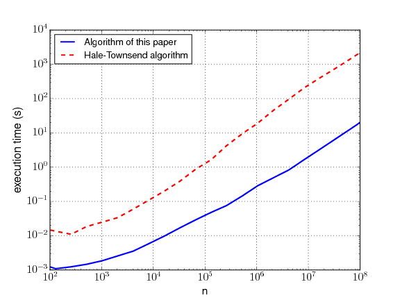
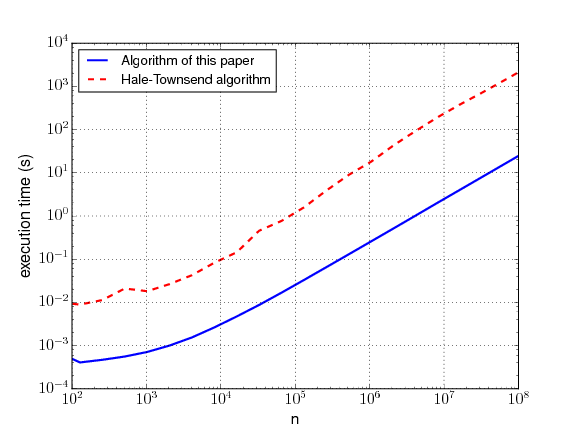
Figure 3: A comparison of the running time of the algorithm of Section 2 for the calculation of Gauss-Jacobi quadrature rules with the algorithm of Hale-Townsend [21]. In the experiments whose results are shown on the left, the parameters were taken to be $a=0.25$ and $b=0.40$ while in the experiments corresponding to the plot on the right, the parameters were $a=-0.49$ and $b=0.25$.

For $a=0$ and $b=-4/10$ and various values of $n$, we constructed the $n$-point Gauss-Jacobi quadrature rule using both the algorithm of Section 2 and the Julia implementation [20] of the Hale-Townsend algorithm made available by the authors of [21]. For each chosen value of $n$, we measured the relative difference in $100$ randomly selected weights. Unfortunately, in some cases [20] loses a small amount of accuracy when evaluating quadrature weights corresponding to quadrature nodes near the points $\pm 1$. Accordingly, when choosing random nodes, we omitted those corresponding to the $20$ quadrature nodes closest to each of the points $\pm 1$. We note that the loss of accuracy in [20] is merely a problem with that particular implementation of the Hale-Townsend algorithm and not with the underlying scheme. Indeed, the MATLAB implementation of the Hale-Townsend algorithm included with the Chebfun package [9] does not suffer from this defect. We did not compare against the MATLAB version of the code because it is somewhat slower than the Julia implementation. Table 3 reports the results. We began our comparison with $n=101$ because when $n\leq 100$, the Hale-Townsend code combines the well-known three-term recurrence relations satisfied by solutions of Jacobi’s differential equation and Newton’s method to construct the $n$-point Gauss-Jacobi quadrature rule. This is also the strategy we recommend for constructing Gauss-Jacobi rules when $n$ is small.

For different pairs of the parameters $a$ and $b$ and various values of $n$, we used [20] and the algorithm of this paper to produce $n$-point Gauss-Jacobi quadrature rules and compared the running times of these two algorithms. Figure 3 displays the results.

$n$	Running time of the	Running time of	Ratio	Maximum relative
	algorithm of Section 2	the algorithm of [21]		error in weights
101	4.45$\times 10^{-04}$	9.62$\times 10^{-03}$	2.15$\times 10^{+01}$	4.47$\times 10^{-15}$
128	4.00$\times 10^{-04}$	9.26$\times 10^{-03}$	2.31$\times 10^{+01}$	4.78$\times 10^{-15}$
256	4.54$\times 10^{-04}$	1.15$\times 10^{-02}$	2.54$\times 10^{+01}$	5.76$\times 10^{-15}$
512	5.34$\times 10^{-04}$	2.14$\times 10^{-02}$	4.00$\times 10^{+01}$	7.04$\times 10^{-15}$
1,024	6.64$\times 10^{-04}$	2.27$\times 10^{-02}$	3.41$\times 10^{+01}$	6.26$\times 10^{-15}$
2,048	8.86$\times 10^{-04}$	3.00$\times 10^{-02}$	3.39$\times 10^{+01}$	6.99$\times 10^{-15}$
4,096	1.31$\times 10^{-03}$	5.28$\times 10^{-02}$	4.01$\times 10^{+01}$	7.45$\times 10^{-15}$
8,192	2.15$\times 10^{-03}$	8.76$\times 10^{-02}$	4.06$\times 10^{+01}$	7.99$\times 10^{-15}$
16,384	3.80$\times 10^{-03}$	2.68$\times 10^{-01}$	7.07$\times 10^{+01}$	1.07$\times 10^{-14}$
32,768	7.03$\times 10^{-03}$	4.45$\times 10^{-01}$	6.33$\times 10^{+01}$	8.29$\times 10^{-15}$
65,536	1.35$\times 10^{-02}$	7.91$\times 10^{-01}$	5.85$\times 10^{+01}$	9.23$\times 10^{-15}$
131,072	2.64$\times 10^{-02}$	1.61$\times 10^{+00}$	6.10$\times 10^{+01}$	1.04$\times 10^{-14}$
262,144	5.22$\times 10^{-02}$	4.14$\times 10^{+00}$	7.92$\times 10^{+01}$	8.44$\times 10^{-15}$
524,288	1.03$\times 10^{-01}$	9.06$\times 10^{+00}$	8.74$\times 10^{+01}$	1.09$\times 10^{-14}$
1,048,576	2.06$\times 10^{-01}$	1.80$\times 10^{+01}$	8.73$\times 10^{+01}$	1.29$\times 10^{-14}$
2,097,152	4.11$\times 10^{-01}$	4.26$\times 10^{+01}$	1.03$\times 10^{+02}$	1.26$\times 10^{-14}$
4,194,304	8.24$\times 10^{-01}$	9.27$\times 10^{+01}$	1.12$\times 10^{+02}$	1.16$\times 10^{-14}$
8,388,608	1.65$\times 10^{+00}$	1.95$\times 10^{+02}$	1.17$\times 10^{+02}$	1.36$\times 10^{-14}$
16,777,216	3.30$\times 10^{+00}$	3.86$\times 10^{+02}$	1.16$\times 10^{+02}$	1.43$\times 10^{-14}$
33,554,432	6.59$\times 10^{+00}$	7.33$\times 10^{+02}$	1.11$\times 10^{+02}$	1.43$\times 10^{-14}$
67,108,864	1.31$\times 10^{+01}$	1.42$\times 10^{+03}$	1.08$\times 10^{+02}$	1.48$\times 10^{-14}$
100,000,000	1.96$\times 10^{+01}$	2.10$\times 10^{+03}$	1.07$\times 10^{+02}$	1.77$\times 10^{-14}$

Table 3: The results of an experiment comparing the algorithm of [21] for the numerical calculation of Gauss-Jacobi quadrature rules with that of Section 2. In these experiments, the parameters were taken to be $a=0$ and $b=-4/10$. All times are in seconds.

6.3 The Jacobi transform

In these experiments, we measured the speed and accuracy of the algorithm of Section 5 for the application of the Jacobi transform and its inverse.

We did so in part by comparison with the algorithm of Slevinsky [33] for applying the Chebyshev-Jacobi and Jacobi-Chebyshev transforms. The Chebyshev-Jacobi transform is the map which takes the coefficients of the Chebyshev expansion of a function to the coefficients in its Jacobi expansion and the Jacobi-Chebyshev transform is the inverse of this map. Although these are not the transforms we apply, the Jacobi transform can be implemented easily by combining the method of [33] with the nonuniform fast Fourier transform (see, for instance, [23] and [22] for an approach of this type for applying the Legendre transform and its inverse). Other methods for applying the Jacobi transform, some of which have lower asymptotic complexity than the algorithm of [33] and the approach of this paper, are available. Butterfly algorithms such as [27, 28, 30] allow for the application of the Jacobi transform and various related mappings in $\mathcal{O}\left(n\log(n)\right)$ operations; however, existing methods are either numerically unstable or they require expensive precomputation phases with higher asymptotic complexity. The Alpert-Rokhlin method [1] uses a multipole-like approach to apply the Chebyshev-Legendre and Legendre-Chebyshev transforms in $\mathcal{O}\left(n\right)$ operations. The Legendre transform can be computed in $\mathcal{O}\left(n\log(n)\right)$ operations by combining this algorithm with the fast Fourier transform. This approach is extended in [25] in order to compute expansions in Gegenbauer polynomials in $\mathcal{O}(n\log(n))$ operations. It seems likely that these methods can be extended to compute expansions in more general classes of Jacobi polynomials; however, to the authors’ knowledge no such algorithm has been published and algorithms from this class require expensive precomputations. A further discussion of methods for the application of the Jacobi transform and related mappings can be found in [33].

$n$	Forward Jacobi	Chebyshev-Jacobi	Ratio
	transform time	transform time
	algorithm of Section 5	algorithm of [33]
10	6.78$\times 10^{-07}$	1.96$\times 10^{-04}$	2.88$\times 10^{+02}$
16	5.10$\times 10^{-07}$	1.78$\times 10^{-04}$	3.49$\times 10^{+02}$
32	2.21$\times 10^{-05}$	1.99$\times 10^{-04}$	9.00$\times 10^{+00}$
64	3.08$\times 10^{-05}$	3.86$\times 10^{-04}$	1.25$\times 10^{+01}$
128	2.74$\times 10^{-05}$	5.65$\times 10^{-04}$	2.05$\times 10^{+01}$
256	4.52$\times 10^{-05}$	8.33$\times 10^{-04}$	1.84$\times 10^{+01}$
512	8.46$\times 10^{-05}$	2.77$\times 10^{-03}$	3.27$\times 10^{+01}$
1,024	1.56$\times 10^{-04}$	5.71$\times 10^{-03}$	3.64$\times 10^{+01}$
2,048	3.44$\times 10^{-04}$	1.53$\times 10^{-02}$	4.46$\times 10^{+01}$
4,096	9.41$\times 10^{-04}$	2.75$\times 10^{-02}$	2.92$\times 10^{+01}$
8,192	2.35$\times 10^{-03}$	8.75$\times 10^{-02}$	3.70$\times 10^{+01}$
16,384	6.08$\times 10^{-03}$	2.12$\times 10^{-01}$	3.48$\times 10^{+01}$
32,768	1.43$\times 10^{-02}$	5.08$\times 10^{-01}$	3.55$\times 10^{+01}$
65,536	2.92$\times 10^{-02}$	9.91$\times 10^{-01}$	3.39$\times 10^{+01}$
131,072	7.36$\times 10^{-02}$	3.25$\times 10^{+00}$	4.42$\times 10^{+01}$
262,144	1.35$\times 10^{-01}$	4.47$\times 10^{+00}$	3.30$\times 10^{+01}$
524,288	4.50$\times 10^{-01}$	1.54$\times 10^{+01}$	3.43$\times 10^{+01}$
1,048,576	1.05$\times 10^{+00}$	2.28$\times 10^{+01}$	2.15$\times 10^{+01}$
2,097,152	2.72$\times 10^{+00}$	6.70$\times 10^{+01}$	2.45$\times 10^{+01}$
4,194,304	8.55$\times 10^{+00}$	1.44$\times 10^{+02}$	1.69$\times 10^{+01}$
8,388,608	1.74$\times 10^{+01}$	3.33$\times 10^{+02}$	1.91$\times 10^{+01}$
16,777,216	3.67$\times 10^{+01}$	5.80$\times 10^{+02}$	1.57$\times 10^{+01}$
33,554,432	7.92$\times 10^{+01}$	1.61$\times 10^{+03}$	2.03$\times 10^{+01}$
67,108,864	1.66$\times 10^{+02}$	3.03$\times 10^{+03}$	1.81$\times 10^{+01}$
100,000,000	1.52$\times 10^{+02}$	5.25$\times 10^{+03}$	3.43$\times 10^{+01}$

Table 4: A comparison of the time required to apply the Chebyshev-Jacobi transform using the algorithm of [33] with the time required to apply the forward Jacobi transform via the algorithm of Section 5. Here, $a$ was taken to be $1/4$ and $b$ was $-4/10$. All times are in seconds.

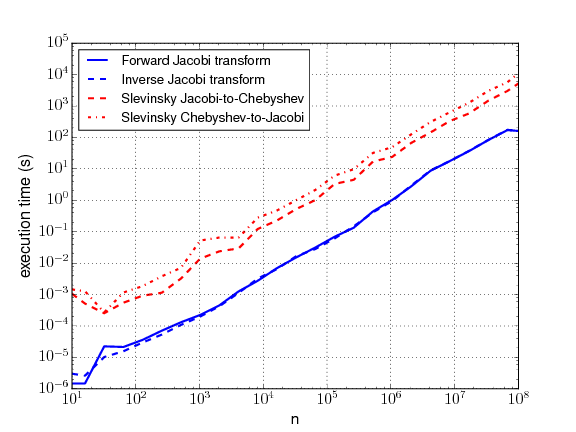
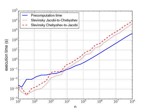
Figure 4: On the left is a comparison of the time required to apply the Chebyshev-Jacobi transform and its inverse using the algorithm of [33] with the time required to apply the forward and inverse Jacobi transforms via the algorithm of Section 5. On the right is a comparison of the cost of the precomputations for the procedure of Section 5 with the time required to apply the Jacobi-Chebyshev map and its inverse via the algorithm of [33]. In these experiments, $a$ was taken to be $-1/4$ and $b$ was $0$.

Figure 4 and Table 4 report the results of our comparisons with the Julia implementation [32] of Slevinsky’s algorithm. The graph on the left side of Figure 4 compares the time taken by the algorithm of Section 5 to apply the Jacobi transform and its inverse with the time required to apply the Chebyshev-Jacobi mapping and its inverse via [33], while the graph on the right compares the time required by our precomputation procedure with the time required to apply the Chebyshev-Jacobi mapping and it inverse with Slevinsky’s algorithm. We observe that cost of our algorithm, including the precomputation stage, is less than that of [33] at relatively modest orders. Moreover, Figure 4 strongly suggests that the asymptotic running time of our algorithm for the application of the Jacobi transform is similar to the $O\left(n\log^{2}\left(n\right)/\log\left(\log\left(n\right)\right)\right)$ complexity of Slevinsky’s algorithm.

Owing to the loss of accuracy which arises when the Formula (2) is used to evaluate Jacobi polynomials of large degrees, we expect the error in the Jacobi transform of Section 5 to increase as the order of the transform increases. This is indeed the case, at least when it is applied to functions whose Jacobi coefficients do not decay or decay slowly. However, when the transform is applied to smooth functions, whose Jacobi coefficients decay rapidly, the errors grow more slowly than in the general case. This is the same as the behavior of the algorithms [33] and [23]. We carried out a further set of experiments to illustrate this effect. In particular, we applied the forward Jacobi transform followed by the inverse Jacobi transform to vectors which decay at various rates. We constructed test vectors by choosing their entries from a Gaussian distribution and then scaling them so as to achieve a desired rate of decay. Figure 5 reports the results. It also contains a plot of the rank of the matrix (107) as a function of $n$ for various pairs of the parameters $a$ and $b$.

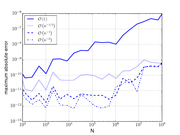
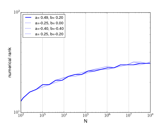
Figure 5: On the left are plots of the largest absolute errors which occurs when the composition of the inverse and forward Jacobi transforms of Section 5 are applied to vectors whose coefficients decay at varying rates. For these experiments, $a=-1/4$ and $b=0$. On the right are plots of the rank of the matrix (107) as a function of $N_{\mbox{\tiny max}}$ for various values of the parameters $a$ and $b$.

We also compared the time required to apply the forward Jacobi transform via the algorithm of Section 5 with the time required to do so by evaluating the matrix $\mathcal{J}_{n}^{(a,b)}$ using the well-known three-term recurrence relations and then applying it directly (we refer to this as the “brute force technique”). This is the methodology we recommend for transforms of small orders. In these experiments, the parameters $a$ and $b$ were taken to be $a=1/4$ and $b=-1/3$. Figure 6 shows the results.

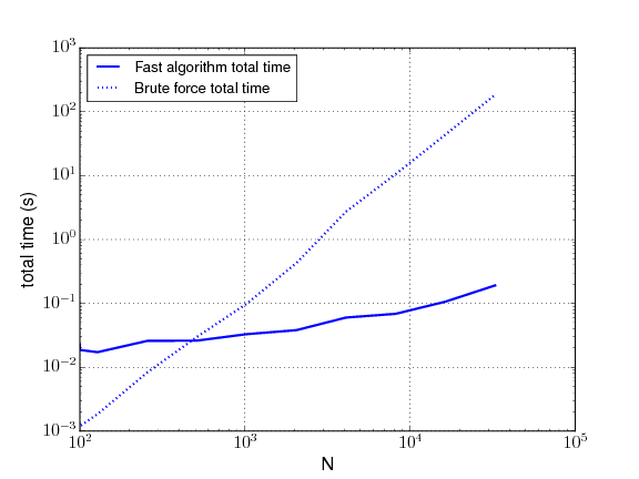
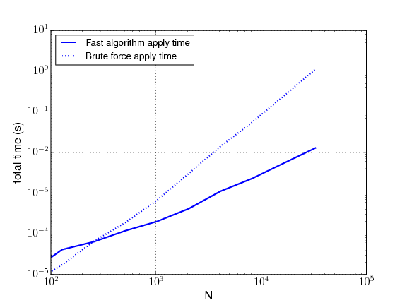
Figure 6: A comparison of the time take to apply the Forward Jacobi transform via “brute force” with the time required to do so via the algorithm of Section 5. On the left is a plot of the total time taken. For the algorithm of Section 5 this includes the time taken by the precomputation phase, while for “brute force” technique this includes the time required to evaluate the entries of the matrix $\mathcal{J}_{n}^{(a,b)}$ via three-term recurrence relations. On the right is a comparison of the application times only. Here, the parameters are $a=1/4$ and $b=-1/3$.

7 Conclusion and Further Work

We have described a suite of fast algorithms for forming and manipulating expansions in Jacobi polynomials. They are based on the well-known fact that Jacobi’s differential equation admits a nonoscillatory phase function. Our algorithms use numerical methods, rather than asymptotic expansions, to evaluate the phase function and other functions related to it. We do so in part because existing asymptotic expansions for the phase function do not suffice for our purposes (they either not sufficiently accurate or they are not numerically viable), but also because such techniques can be easily applied to any family of special functions satisfying a second order differential equation with nonoscillatory coefficients. We will report on the application of our methods to other families of special functions at a later date.

It would be of some interest to accelerate the procedure of Section 3 for the construction of the nonoscillatory phase and amplitude functions. There are a number obvious mechanisms for doing so, but perhaps the most promising is the observation that the ranks of matrices with entries

$$\psi^{(a,b)}(t_{j},\nu_{k})$$ (121)

and

$$M^{(a,b)}(t_{j},\nu_{k})$$ (122)

are quite low — indeed, in the experiments of this paper they were never observed to be larger than $40$. This means that, at least in principle, the nonoscillatory phase and amplitude can be represented via $40\times 40$ matrices, and that a carefully designed spectral scheme which takes this into account could compute the $40$ required solutions of the ordinary differential equation (41) extremely efficiently.

The authors are investigating such an approach to the construction of $\psi^{(a,b)}$ and $M^{(a,b)}$.

As the parameters $a$ and $b$ increase beyond $\frac{1}{2}$, our algorithms become less accurate, and they ultimately fail. This happens because for values of the parameters $a$ and $b$ greater than $\frac{1}{2}$, the Jacobi polynomials have turning points and the crude approximation (14) becomes inadequate. An obvious remedy is to use a more sophisticated approximations for $\psi^{(a,b)}$ and $M^{(a,b)}$. The authors will report on extensions of this work which make use of such an approach at a later date.

8 References

References

- [1] Alpert, B. K., and Rokhlin, V. A fast algorithm for the evaluation of Legendre expansions. SIAM Journal on Scientific and Statistical Computing 12, 1 (1991), 158–179.
- [2] Baratella, P., and Gatteschi, L. The bounds for the error term of an asymptotic approximation of Jacobi polynomials. In Orthogonal Polynomials and their Applications, Lecture Notes in Mathematics 1329. 1988, pp. 203–221.
- [3] Bogaert, I. Iteration-free computation of Gauss-Legendre quadrature nodes and weights. SIAM Journal on Scientific Computing 36 (2014), A1008–A1026.
- [4] Bogaert, I., Michiels, B., and Fostier, J. computation of Legendre polynomials and Gauss-Legendre nodes and weights for parallel computing. SIAM Journal on Scientific Computing 34 (2012), C83–C101.
- [5] Bremer, J. On the numerical calculation of the roots of special functions satisfying second order ordinary differential equations. SIAM Journal on Scientific Computing 39 (2017), A55–A82.
- [6] Candès, E., Demanet, L., and Ying, L. Fast computation of fourier integral operators. SIAM Journal on Scientific Computing 29, 6 (2007), 2464–2493.
- [7] Cheng, H., Gimbutas, Z., Martinsson, P., and Rokhlin, V. On the compression of low rank matrices. SIAM Journal on Scientific Computing 26 (2005), 1389–1404.
- [8] NIST Digital Library of Mathematical Functions. http://dlmf.nist.gov/, Release 1.0.13 of 2016-09-16. F. W. J. Olver, A. B. Olde Daalhuis, D. W. Lozier, B. I. Schneider, R. F. Boisvert, C. W. Clark, B. R. Miller and B. V. Saunders, eds.
- [9] Driscoll, T. A., Hale, N., and Trefethen, L. N. Chebfun Guide. Pafnuty Publications, Oxford, 2014.
- [10] Dunster, T. M. Asymptotic approximations for the Jacobi and ultraspherical polynomials, and related functions. Methods and Applications of Analysis 6 (1999), 281–316.
- [11] Engquist, B., and Ying, L. A fast directional algorithm for high frequency acoustic scattering in two dimensions. Commun. Math. Sci. 7, 2 (2009), 327–345.
- [12] Erdélyi, A., et al. Higher Transcendental Functions, vol. I. McGraw-Hill, 1953.
- [13] Erdélyi, A., et al. Higher Transcendental Functions, vol. II. McGraw-Hill, 1953.
- [14] Frenzen, C., and Wong, R. A uniform asymptotic expansion of the Jacobi polynomials with error bounds. Canadian Journal of Mathematics 37 (1985), 979–1007.
- [15] Frigo, M., and Johnson, S. G. The design and implementation of FFTW3. Proceedings of the IEEE 93, 2 (2005), 216–231. Special issue on “Program Generation, Optimization, and Platform Adaptation”.
- [16] Glaser, A., Liu, X., and Rokhlin, V. A fast algorithm for the calculation of the roots of special functions. SIAM Journal on Scientific Computing 29 (2007), 1420–1438.
- [17] Greengard, L. Spectral integration and two-point boundary value problems. SIAM Journal of Numerical Analysis 28 (1991), 1071–1080.
- [18] Greengard, L., and Lee, J.-Y. Accelerating the nonuniform fast fourier transform. SIAM Review 46, 3 (2004), 443–454.
- [19] Hahn, E. Asymptotik bei Jacobi-polynomen und Jacobi-funktionen. Mathematische Zeitschrift 171 (1980), 201–226.
- [20] Hale, N., and Townsend, A. Fast Gauss Quadrature library. http://github.com/ajt60gaibb/FastGaussQuadrature.jl.
- [21] Hale, N., and Townsend, A. Fast and accurate computation of Gauss-Legendre and Gauss-Jacobi quadrature nodes and weights. SIAM Journal on Scientific Computing 35 (2013), A652–A674.
- [22] Hale, N., and Townsend, A. A fast, simple and stable Chebyshev-Legendre transform using an asymptotic formula. SIAM Journal on Scientific Computing 36 (2014), A148–A167.
- [23] Hale, N., and Townsend, A. A fast FFT-based discrete Legendre transform. IMA Journal of Numerical Analysis 36 (2016), 1670–1684.
- [24] Halko, N., Martinsson, P. G., and Tropp, J. A. Finding structure with randomness: Probabilistic algorithms for constructing approximate matrix decompositions. SIAM Review 53 (2011), 217–288.
- [25] Keiner, J. Computing with expansions in Gegenbauer polynomials. SIAM Journal on Scientific Computing 31 (2009), 2151–2171.
- [26] Li, Y., and Yang, H. Interpolative butterfly factorization. SIAM Journal on Scientific Computing 39, 2 (2017), A503–A531.
- [27] Li, Y., Yang, H., Martin, E., Ho, K. L., and Ying, L. Butterfly factorization. SIAM Journal on Multiscale Modeling and Simulation 13 (2015), 714–732.
- [28] Li, Y., Yang, H., and Ying, L. Multidimensional butterfly factorization. Applied and Computational Harmonic Analysis 44, 3 (2018), 737 – 758.
- [29] Merkle, M. Completely monotone functions: a digest. In Analytic Number Theory, Approximation Theory, and Special Functions. Springer, New York, NY, 2014.
- [30] O’Neil, M., Woolfe, F., and Rokhlin, V. An algorithm for the rapid evaluation of special function transforms. Applied and Computational Harmonic Analysis 28 (2010), 203–226.
- [31] Ruiz-Antolin, D., and Townsend, A. A nonuniform fast Fourier transform based on low rank approximation. SIAM Journal on Scientific Computing 40 (2018), A529–A547.
- [32] Slevinsky, M. Fast Transforms library. https://github.com/MikaelSlevinsky/FastTransforms.jl.
- [33] Slevinsky, R. On the use of Hahn’s asymptotic formula and stabilized recurrence for a fast, simple and stable Chebyshev-Jacobi transform. IMA Journal of Numerical Analysis 38 (2017), 102–124.
- [34] Szegö, G. Orthogonal Polynomials. American Mathematical Society, Providence, Rhode Island, 1959.
- [35] Trefethen, N. Approximation Theory and Approximation Practice. Society for Industrial and Applied Mathematics, 2013.
- [36] Watson, G. N. A Treatise on the Theory of Bessel Functions, second ed. Cambridge University Press, New York, 1995.
- [37] Yang, H. A unified framework for oscillatory integral transform: When to use NUFFT or butterfly factorization? preprint (2018).