The Electric Two-echelon Vehicle Routing Problem

Abstract

Two-echelon distribution systems are attractive from an economical standpoint and help to keep large vehicles out of densely populated city centers. Large trucks can be used to deliver goods to intermediate facilities in accessible locations, whereas smaller vehicles allow to reach the final customers. Due to their reduced size, pollution, and noise, multiple companies consider using an electric fleet of terrestrial or aerial vehicles for last-mile deliveries.

Route planning in multi-tier logistics leads to notoriously difficult problems. This difficulty is accrued in the presence of an electric fleet since each vehicle operates on a smaller range and may require planned visits to recharging stations. To study these challenges, we introduce the electric two-echelon vehicle routing problem (E2EVRP) as a prototypical problem. We propose a large neighborhood search (LNS) metaheuristic as well as an exact mathematical programming algorithm, which uses decomposition techniques to enumerate promising first-level solutions in conjunction with bounding functions and route enumeration for the second-level routes. These algorithms produce optimal or near-optimal solutions for the problem and allow us to evaluate the impact of several defining features of optimized battery-powered distribution networks.

We created representative E2EVRP benchmark instances to simulate realistic metropolitan areas. In particular, we observe that the detour miles due to recharging decrease proportionally to $1/\rho^{x}$ with $x\approx 5/4$ as a function of the charging stations density $\rho$; e.g., in a scenario where the density of charging stations is doubled, recharging detours are reduced by 58%. Finally, we evaluate the trade-off between battery capacity and detour miles. This estimate is critical for strategic fleet-acquisition decisions, in a context where large batteries are generally more costly and less environment-friendly.

1 Introduction

Nowadays, as technology for electric mobility progresses, multi-tier delivery schemes are naturally destined to make use of electric vehicles, and multiple companies have, in practice, already operated this transition (Foltyński 2014). Yet, electric vehicles also pose specific challenges, due to their limited autonomy, smaller capacity, and the possible need of planned visits to charging stations. Moreover, whereas early charging technologies required several hours for a full recharge, recent developments of fast-charging or battery-swap stations (Yang and Sun 2015, Hof et al. 2017, Keskin and Çatay 2018) allow energy replenishment in half an hour. The growing adoption of these technologies allows en-route recharging (e.g., during lunch breaks) in metropolitan distribution systems, as well as the use of cheaper lightweight vehicles (Perboli et al. 2018a, Perboli and Rosano 2018) with smaller batteries. Last but not the least, the study on battery-powered distribution is not limited to terrestrial vehicles, but also meets critical applications in last-mile distribution using aerial vehicles (i.e., drones – Poikonen et al. 2017 and Wang et al. 2017b), which typically have a smaller autonomy.

To focus on these challenges, we introduce the E2EVRP as a prototypical problem. It is a natural extension of the two-echelon vehicle routing problem (2EVRP) in which electric vehicles are used on the second echelon. Given a geographically-dispersed set of customers demanding an amount of a single commodity, a set of satellites (intermediate facilities), a set of charging stations, and a central depot where the commodity is kept, the E2EVRP seeks least-cost delivery routes to transport the commodity from the depot to the satellites with conventional vehicles (first-level), and from the satellites to the customers using an electric fleet (second-level). Some additional rules must be satisfied with respect to the basic 2EVRP:

• Electric vehicles have a limited driving range, which can be fully replenished at a charging station;

• Each second-level route originates at a satellite, visits a sequence of customers and possibly some recharging stations, and returns to the same satellite;

• Each satellite also hosts a charging station at its location;

• Charging stations can be used multiple times, but a consecutive visit to two charging stations in a second-level route is prohibited.

The cost of the solution, to be minimized, includes a fixed cost for each vehicle in use, as well as driving costs proportional to the distance traveled.

To solve this problem, we introduce a LNS-based metaheuristic which combines a restricted set of destruction and reconstruction operators, a local search procedure, and a fast labeling algorithm to optimize the visits to charging locations. We also propose an exact mathematical programming algorithm, which uses a decomposition technique to enumerate promising first-level solutions along with bounding functions and route enumeration for the second level, using problem-tailored pricing algorithms. These two methods can be viewed as extensions of the approaches of Breunig et al. (2016) and Baldacci et al. (2013) for the classical 2EVRP, in which specialized route evaluation techniques, labeling algorithms and dominance strategies have been integrated to efficiently manage the selection of recharging stations for the electric vehicles.

Not only do these algorithms allow to find optimal or near-optimal solutions for the E2EVRP, and thus respond to the need of advanced algorithms for future city-logistics planning, but they also open the way to an analysis of several defining features of optimized battery-powered city-distribution networks. To that end, we created new datasets which simulate the general characteristics of a metropolitan area, and examine the impact of the density of the charging station network and the capacity of the vehicles’ batteries on the cost-efficiency of the optimal solutions of the problem.

The remainder of this paper is organized as follows. Section 2 reviews the related literature and Section 3 formally describes the problem. Then, Sections 4 and 5 describe, respectively, the proposed exact and heuristic algorithms. Section 6 reports our computational experiments and sensitivity analyses, and Section 7 concludes.

2 Related Literature

We review the existing solution algorithms for the 2EVRPs, discuss the recent studies dedicated to routing optimization for vehicles with alternative fuels, and finally examine the use of en-route recharging in recent studies and applications.

Two-echelon vehicle routing problems. Several early studies focused on mathematical programming solution techniques for the 2EVRP. Gonzalez-Feliu et al. (2008) were the first to describe a branch-and-cut algorithm based on a commodity flow formulation that solved instances with up to $32$ customers and $2$ satellites. The method of Gonzalez-Feliu et al. (2008) was improved by Perboli et al. (2010) and Perboli et al. (2011) by adding valid inequalities in a cutting plane fashion. Optimal solutions for instances with up to $32$ customers and $2$ satellites were found by the method of Perboli et al. (2011). Jepsen et al. (2012) described a branch-and-cut algorithm based on a new mathematical formulation and different valid inequalities. Exact algorithms were also designed by Baldacci et al. (2013) and by Santos et al. (2015). Santos et al. described a branch-and-cut-and-price algorithm for the 2EVRP that relies on a reformulation based on the $q$-routes relaxation proposed for the capacitated vehicle routing problem (CVRP) by Christofides et al. (1981). Baldacci et al. proposed an exact method for solving the 2EVRP based on a set partitioning formulation with side constraints. They described a bounding procedure that is used by the exact algorithm to decompose the problem into a limited set of multi-depot capacitated vehicle routing problems with side constraints. The optimal 2EVRP solution is obtained by solving the set of MDCVRPs generated. The method was tested on 207 instances, taken both from the literature and newly generated, with up to 100 customers and 6 satellites. The results obtained by Baldacci et al. (2013) show that their exact algorithm outperforms the existing methods from the papers described above. Finally, Perboli et al. (2018b) recently found new valid inequalities for the 2EVRP. Using these inequalities within a branch-and-cut algorithm allowed to solve several new instances with up to 50 customers.

The number of heuristics, metaheuristics and case studies focused on multi-echelon vehicle routing problems has also rapidly grown in the last decade. The surveys by Cuda et al. (2015) and Schiffer et al. (2018) capture well the breadth of this line of research. The former covers different two-echelon structured transportation problems: two-echelon location routing problems, 2EVRPs and truck and trailer routing problems. The latter focuses on vehicle routing problems and location routing problems with intermediate stops, dedicated to replenishment, refueling or idling. Among the most recent contributions in this domain, Zeng et al. (2014) proposed a greedy randomized adaptive search procedure with a route-first cluster-second splitting algorithm and a variable neighborhood descent for the 2EVRP. Their results are promising, but the algorithm was only tested on the smaller benchmark instances with up to 50 delivery points. Breunig et al. (2016) introduced a LNS for 2EVRPs and the two-echelon location routing problem with single depot (2ELRPSD). The method uses six destroy and one repair operator as well as some well-known local search procedures. It finds or improves 95% of the best known solutions for the classical benchmark instances. Given the efficiency and the effectiveness of this method, the same general structure has been used for the heuristic proposed in this paper, in addition with multiple improvements and adaptations to account for the specificities of electric vehicles. Later on, Wang et al. (2017a) studied an extension of the 2EVRP with stochastic demands, described as a stochastic program with recourse. A genetic algorithm was proposed, and the results on the problem with stochastic demands were compared to the best known deterministic solutions.

Electric vehicle routing, en-route recharging and battery swaps. Over the last decade, research has also rapidly progressed on vehicle routing problems with alternative propulsion modes: electric or hybrid. As generally reflected in the surveys of Montoya (2016), Pelletier et al. (2016) and Schiffer et al. (2018), many of these studies consider possible en-route recharging or battery swaps to overcome the range limitations of electric vehicles.

Conrad and Figliozzi (2011) were amongst the first to consider optimization techniques for electric vehicles and possible recharging stops. In the proposed recharging VRP, batteries can be charged at customer locations subject to additional costs. Other studies were focused on VRPs considering different aspects of environment-friendly transport. In particular, Erdogan and Miller-Hooks (2012) proposed the green vehicle routing problem (GVRP), involving battery-powered vehicles with possible en-route recharging at dedicated stations, and evaluated the implications of refueling-stations availability and dispersion.

After these seminal works, the literature progressed towards more intricate problem variants and solution methods. Schneider et al. (2014) introduced additional time-window constraints for customer deliveries as well as recharging delays. New benchmark instances were introduced, and solved by means of a hybrid heuristic combining variable neighborhood search (VNS) and tabu search (TS). Desaulniers et al. (2016) developed an exact method based on branch-price-and-cut, and presented computational results for the same benchmark instances.

Moreover, to progress towards real applications and improve the accuracy of the studies, other important characteristics of real delivery networks have been considered. Heterogeneous fleets with different propulsion modes were studied in Felipe et al. (2014), jointly with a heterogeneous set of recharging stations with different cost and recharging time. Goeke and Schneider (2015) considered a mix of conventional and electric vehicles, evaluating the energy consumption of an electric vehicle as a function of speed, gradient and cargo load distribution. Hiermann et al. (2016) proposed the electric fleet size and mix problem with fixed costs and time windows (EFSMFTW), in which the deliveries can be performed with a mix of vehicle types, differing in their acquisition cost, freight capacity, and battery size. Experiments were conducted with a branch-and-price algorithm and a hybrid heuristic. This research was extended in Hiermann et al. (2019) to study the impact of additional plug-in hybrid vehicles. Keskin and Çatay (2016) introduced an adaptive large neighborhood search (ALNS) for a problem variant in which partial recharging is allowed.

In a recent case study, Wang et al. (2017c) stressed several interesting facts regarding the use of large battery powered commercial vehicles. They show that in the real-world transit network based in Davis, California, range anxiety can be mitigated by adopting good recharging strategies, and that several companies adapt much stricter range limits than the theoretical ones (typically half of the range) to extend battery life cycles. Finally, they indicate a list of case studies in which battery swapping has been applied to electric bus transit systems, a strategy which is justified by the fact that fast charging techniques can significantly extend vehicle ranges within only five to ten minutes of charging. Other recent works have proposed to optimize fast or partial charging strategies. In particular, Schiffer and Walther (2017a) introduced the electric location routing problem with time windows and possible partial recharging stops, whereas Keskin and Çatay (2018) extended the electric vehicle routing problem with time windows (EVRPTW) with different types of stations (super-fast, fast, and normal ones) for en-route recharging.

Real-world applications of en-route recharging. As early as 2008, electric buses were installed for the Beijing Olympic Games. Each bus, of a capacity of 50 seats, can undergo battery swapping up to three times a day (EV World 2008). Similarly, fully electric public transit buses have been operating in Vienna, Austria for several years now. These buses stop for approximately 15 minutes at the end of their route to traverse the inner city and recharge the batteries with an overhead system multiple times a day (Wr. Linien 2013). Schiffer et al. (2016) also recently established a case study of “TEDi Logistik GmbH & Co. KG”, which provides freight transportation services and relies on two electric vehicles. They concluded that the operations would be significantly improved if fast-charging stations were additionally available at a few customers locations for en-route recharging, therefore allowing to reach locations located further than 70km from the depot. Finally, JD.com, one of China’s biggest e-commerce companies, is replacing its existing fleet with fully electric vehicles (John 2017). Seeing the need for it, they recently launched a contest for optimization algorithms capable of routing vehicles with en-route recharging (JD.com 2018).

Our study shares the same objectives as many aforementioned papers: bridging the gap between academic electric VRPs and real problem attributes. The current literature on electric vehicles has only considered simplistic delivery networks with a single depot and a single echelon, but it is well known that city logistics usually involve richer configurations, with interconnected echelons and transportation modes. Moreover, the restricted range of the electric vehicles and their possible need for en-route recharging bring new challenges which have to be considered when selecting intermediate facilities (i.e., satellite) locations. We therefore propose to study the impact of electrical fleets in second-level routes, in a two-echelon delivery setting, where electric vehicles are likely to be needed.

3 Problem Description

The E2EVRP addressed in this paper can be formally described as follows.

A mixed graph $G=(N,E,A)$ is given, where the vertex set $N$ is partitioned as $N=\{0\}\cup N_{S}\cup N_{C}\cup N_{R}$. Vertex $0$ represents the depot, $N_{S}=\{1,2,\dots,n_{s}\}$ represents $n_{s}$ satellites, $N_{C}=\{n_{s}+1,\dots,n_{s}+n_{c}\}$ represents $n_{c}$ customers, and $N_{R}=\{n_{s}+n_{c}+1,\dots,n_{s}+n_{c}+n_{r}\}$ represents $n_{r}$ charging stations. The edge set $E$ is defined as $E=\{\{0,j\}\,:\,j\in N_{S}\}\cup\{\{i,j\}:i,j\in N_{S},i<j\}$ and the arc set $A$ as $A=\{(i,j)\,:\,i,j\in N_{S}\cup N_{C}\cup N_{R},i\neq j\}\setminus\{(i,j):i,j\in N_{S}\}\setminus\{(i,j):i,j\in N_{R}\}$. A travel or routing cost $d_{ij}$ is associated with each edge $\{i,j\}\in E$ and with each arc $(i,j)\in A$.

Each customer $i\in N_{C}$ requires a supply of $q_{i}$ units of goods to be delivered from the depot using the following two types of vehicles. A fleet of $m^{1}$ vehicles of capacity $Q_{1}$ located at depot $0$ and a fleet of $m_{k}$ vehicles of capacity $Q_{2}<Q_{1}$ located at satellite $k\in N_{S}$. Moreover, at most $m^{2}\leq\sum_{k\in N_{S}}m_{k}$ second-level vehicles can be used.

A $1^{\text{st}}$-level vehicle route is a simple cycle in $G$ passing through the depot and a subset of satellites such that the total demand delivered is less than or equal to $Q_{1}$. A satellite $k\in N_{S}$ can be visited by more than one $1^{\text{st}}$-level route and has a capacity $B_{k}$ that limits the demand that can be delivered to it.

A $2^{\text{nd}}$-level route is a circuit in $G$ passing through a satellite and a subset of customers and charging stations and such that the total demand of the visited customers does not exceed the vehicle capacity $Q_{2}$ and the following charging station constraints are respected. Each vehicle on the $2^{\text{nd}}$-level has a maximum battery capacity $L$, and a battery consumption $c_{ij}$ is associated with each arc $(i,j)\in A$; the maximum battery consumption of a vehicle without a visit to a charging station is therefore equal to $L$. Charging stations can be visited right after or before a satellite, or in between customers, and, whenever a charging station is visited, a vehicle is fully charged up to level $L$. In the scope of this short-haul problem, we prohibit a consecutive visit to two charging stations.

Fixed costs $U_{1}$ and $U_{2}$ are also associated with the use of $1^{\text{st}}$-level and $2^{\text{nd}}$-level vehicles, respectively. The cost of a route ($1^{\text{st}}$-level or $2^{\text{nd}}$-level) is equal to the sum of the costs of the traversed edges or arcs plus the fixed cost.

The problem asks to design both $1^{\text{st}}$-level and $2^{\text{nd}}$-level routes so that the quantity delivered from each satellite is equal to the quantity received from the depot, each customer is visited exactly once, and the total cost of the routes is minimized.

Multigraph reformulation. The E2EVRP can be reformulated as a routing problem on a multigraph $G^{\prime}=(N^{\prime},E^{\prime},A^{\prime})$, where $N^{\prime}=\{0\}\cup N_{S}\cup N_{C}$ is the vertex set, $E^{\prime}=\{\{0,j\}\,:\,j\in N_{S}\}\cup\{\{i,j\}:i,j\in N_{S},i<j\}$ is the edge set and $A^{\prime}$ is the arc set. Arc set $A^{\prime}$ is used to represent $2^{\text{nd}}$-level routes and is defined as $A^{\prime}=\{(i,j):i,j\in N_{S}\cup N_{C},i\neq j\}\setminus\{(i,j):i,j\in N_{S}\}$. The arc set $A^{\prime}$ also contains the following set of arcs:

• With each arc $(i,j)\in A^{\prime}$ are associated $h(i,j)$ arcs representing the different paths that a $2^{\text{nd}}$-level vehicle can take to go from vertex $i$ to vertex $j$ with at most one charging station visited in between vertices $i$ and $j$.

• A cost $d(i,j,p)$, a consumption $c(i,j,p)$ and a charging station $s(i,j,p)\in N_{R}$ are associated with each arc $(i,j,p)$, $p=1,\dots,h(i,j)$, $\forall(i,j)\in A^{\prime}$. We assume that $s(i,j,p)=0$ if arc $(i,j,p)$ represents the direct path $(i,j)$ without any charging station visited in between $i$ and $j$.

• The cost $d(i,j,p)$ and the consumption $c(i,j,p)$ of arc $(i,j,p)$ are defined as follows:

  $$\left\{\begin{array}[]{ll}d(i,j,p)=d_{ij},\;c(i,j,p)=c_{ij},&\quad\text{ if }s(i,j,p)=0\vspace*{0.2cm}\\ d(i,j,p)=d_{ik}+d_{kj},\;c(i,j,p)=c_{kj},&\quad\text{ if }k=s(i,j,p)\neq 0.\end{array}\right.$$

Multigraph $G^{\prime}$ does not contain any arc $(i,j,p)$ such that $s(i,j,p)=0$ and $c_{ij}>L$, or $k=s(i,j,p)\neq 0$ and $c_{ik}>L$ or $c_{kj}>L$. Notice that for arc $(i,j,p)$ with $s(i,j,p)\neq 0$ value $L-c(i,j,p)$ represents the battery level of the vehicle after arriving at vertex $j$ whereas if $s(i,j,p)=0$, i.e., no charging station is visited in between $i$ and $j$, the battery level at vertex $j$ is equal to $b-c(i,j,p)$, where $b$ is the battery level at vertex $i$.

A $2^{\text{nd}}$-level route for satellite $k\in N_{S}$ in graph $G^{\prime}$ is a simple circuit in $G^{\prime}$ passing through a satellite and a subset of customers and such that (i) the total demand of the visited customers does not exceed the vehicle capacity $Q_{2}$ and (ii) the vehicle leaves satellite $k$ with a consumption equal to 0 (or, equivalently, the vehicle is fully charged) and its consumption at each visited vertices does not exceed the maximum battery capacity $L$.

The following proposition holds.

Proposition 1

There is a one-to-one correspondence between $2^{\text{nd}}$-level routes in $G$ and $2^{\text{nd}}$-level routes in $G^{\prime}$.

Moreover, the set of arcs $A^{\prime}$ can be reduced by means of the following dominance rule.

Proposition 2

An optimal E2EVRP solution cannot contain an arc $(i,j,r_{1})$ if there exists another arc $(i,j,r_{2})$, $r_{1}\neq r_{2}$, such that:

1. $i\in N_{S}$: $d(i,j,r_{1})\geq d(i,j,r_{2})$ and $c(i,j,r_{1})\geq c(i,j,r_{2})$;

2. $i\in N_{C}$: $d(i,j,r_{1})\geq d(i,j,r_{2})$ and $c(i,j,r_{1})\geq c(i,j,r_{2})$, and $c_{ik_{1}}\geq c_{ik_{2}}$, $k_{1}=s(i,j,r_{1})$, $k_{1}\neq 0$, and $k_{2}=s(i,j,r_{2})$, $k_{2}\neq 0$.

4 Solving the E2EVRP to Optimality

The method used to solve the E2EVRP to optimality is based on the exact method proposed by Baldacci et al. (2013) for the 2EVRP. More precisely, we tailored the method described by Baldacci et al. to handle the multigraph $G^{\prime}$ described in Section 3. The exact method consists of the following two main steps.

1. The set of all $1^{\text{st}}$-level routes is generated and a lower bound LB0 on the E2EVRP is computed. The computation of LB0 is based on a integer relaxation that results in a multiple-choice knapsack problem. In computing lower bound LB0, we extended the $ng$-routes relaxation used in Baldacci et al. to the case of our multigraph $G^{\prime}$ (see below).

2. The set of all possible subsets of $1^{\text{st}}$-level routes that could be used in any optimal E2EVRP solution is generated. For each subset of $1^{\text{st}}$-level routes the following steps are executed:

   1. Lower bound LB0 is computed by fixing the selected set of $1^{\text{st}}$-level routes in solution. If the resulting lower bound is greater than or equal to the cost of the best incumbent E2EVRP solution, then the current subset is rejected, otherwise the next step is executed;

   2. The E2EVRP problem obtained by considering only the selected set of $1^{\text{st}}$-level routes is solved to optimality. The resulting problem is a MDCVRP, that is solved using the method proposed by Baldacci and Mingozzi (2009). The optimal solution cost of the E2EVRP corresponds to the minimum solution cost of such MDCVRPs. In solving problem MDCVRP, we extended the procedure used to generate elementary routes described in Baldacci and Mingozzi (2009) to the case of our multigraph $G^{\prime}$.

The procedure is initialized with the best upper bound computed by the heuristic algorithm described in Section 5. In the computational results of Section 6, we will denote with LB1 (LB2) the minimum of the lower bounds computed at Step 2-(i) (Step 2-(ii)) over the set of subsets of $1^{\text{st}}$-level routes. Lower bound LB2 is computed using the lower bounds provided by the method of Baldacci and Mingozzi (2009).

In the following, we describe how we extended the $ng$-routes relaxation to graph $G^{\prime}$ and, for the sake of space, we omit the details of the procedure used to generate elementary routes, which is indeed a straightforward adaptation of the procedure used by Baldacci and Mingozzi (2009).

Pricing ng-routes. The computation of the lower bounds at steps 1, 2-(i) and 2-(ii) and the procedure used to generate elementary routes rely on the use of the $ng$-routes relaxation. In this section, we describe the extension of the relaxation described in Baldacci et al. (2011) to multigraph $G^{\prime}$. We describe the relaxation for a generic satellite $k\in N_{S}$ that, for sake of notation, is denoted with the index 0 in the description reported below.

Let $\Omega(w,j,i,p)$ be the subset of battery consumption values from vertex $j$ to arrive at vertex $i$ with a consumption equal to $w$, with $w\leq L$, when $j$ is visited immediately before $i$ using arc of index $p$ of arc $(j,i)\in A^{\prime}$. Set $\Omega(w,j,i,p)$ is defined as follows:

$$\Omega(w,j,i,p)=\begin{cases}\{w-c_{ji}\}&\text{if }s(j,i,p)=0\text{ and }c_{ji}\leq w\\ \{w^{\prime}:0\leq w^{\prime}+c_{jk}\leq L\}&\text{if }s(j,i,p)=k\neq 0\text{ and }c_{ki}=w\\ \varnothing&\text{otherwise.}\\ \end{cases}$$ (1)

Let $N_{i}\subseteq N_{C}$ be a set of selected customers for vertex $i$ such that $N_{i}\ni i$ and $|N_{i}|\leq\Delta(N_{i})$ ($\Delta(N_{i})$ is an a priori defined parameter). The sets $N_{i}$ allow us to associate with each forward path $P=(0,i_{1},\dots,i_{k})$ in $G^{\prime}$ the subset $\Pi(P)\subseteq V(P)$, $V(P)=\{0,i_{1},\ldots,i_{k-1},i_{k}\}$, containing customer $i_{k}$ and every customer $i_{r}$, $r=1,..,k-1$, of $P$ that belongs to all sets $N_{i_{r+1}},\dots,N_{i_{k}}$ associated with the customers $i_{r+1},\dots,i_{k}$ visited after $i_{r}$. The set $\Pi(P)$ is defined as: $\Pi(P)=\{i_{r}:i_{r}\in\bigcap_{s=r+1}^{k}N_{i_{s}},r=1,\dots,k-1\}\cup\{i_{k}\}$.

A $ng$-path $(NG,q,w,i)$ is a non-necessarily elementary path $P=(0,i_{1},\dots,i_{k-1},i_{k}=i)$ starting from the satellite 0 with an initial consumption equal to 0, visiting a subset of customers (even more than once) of total demand equal to $q$ such that $NG=\Pi(P)$, ending at customer $i$ with a total consumption equal to $w$, and such that $i\notin\Pi(P^{\prime})$, where $P^{\prime}=(0,i_{1},\dots,i_{k-1})$ is an $ng$-path. We denote by $f(NG,q,w,i)$ the cost of the least cost $ng$-path $(NG,q,w,i)$. An $(NG,q,w,i)$-route is an $(NG,q,w,0)$-path where $i$ is the last customer visited before arriving at the satellite.

Functions $f(NG,q,w,i)$ can be computed using dynamic programming (DP). The state space graph $\mathscr{H}=(\mathscr{E},\Psi)$ is defined as follows: $\mathscr{E}=\{(NG,q,w,i):q_{i}\leq q\leq Q_{2},\forall NG\subseteq N_{i}\text{ s.t. }NG\ni i,\,\sum_{j\in NG}q_{j}\leq Q_{2},\allowbreak\forall i\in\{0\}\cup N_{C},\forall w,0\leq w\leq L\}$, $\Psi=\{((NG^{\prime},q^{\prime},w^{\prime},j),(NG,q,w,i))^{p}:\forall(NG^{\prime},q^{\prime},w^{\prime},j)\in\Psi^{-1}(NG,q,w,j,i,p),\allowbreak p=1,\dots,h(j,i),\forall(j,i)\in A^{\prime},\forall(NG,q,w,i)\in\mathscr{E}\}$, where $\Psi^{-1}(NG,q,w,j,i,p)=\{(NG^{\prime},q-q_{i},w^{\prime},j):\forall NG^{\prime}\subseteq N_{j}\text{ s.t. }NG^{\prime}\ni j\text{ and }NG^{\prime}\cap N_{i}={NG\setminus\{i\}},\,\forall w^{\prime}\in\Omega(w,j,i,p)\}$.

The DP recursion for computing $f(NG,q,w,i)$ is:

$$f(NG,q,w,i)=\min_{\begin{subarray}{c}(j,i)\in A^{\prime},\;1\leq p\leq h(j,i)\\ (NG^{\prime},q^{\prime},w^{\prime},j)\in\Psi^{-1}(NG,q,w,j,i,p)\end{subarray}}\left\{f(NG^{\prime},q^{\prime},w^{\prime},j)+d(j,i,p)\right\},\forall(NG,q,w,i)\in\mathscr{E},\vspace*{0.4cm}$$ (2)

using as initial state $f(\{0\},0,0,0)=0$ and $f(\{0\},q,w,0)=\infty$ for $q>0$ and $w>0$. In the computational experiments (Section 6), we set $\Delta(N_{i})=12$, $\forall i\in N_{C}$, and $N_{i}$ contains $i$ and the 11 nearest customers to $i$.

From the experimental analysis presented in Section 6, we observed that this mathematical programming algorithm can solve small and medium size instances to optimality and provide good lower bounds otherwise. Yet, this method requires a good initial upper bound to be truly effective, especially when the problem size grows. To produce these upper bounds, the following section introduces a metaheuristic based on large neighborhood search.

5 Large Neighborhood Search

Our metaheuristic, called LNS-E2E, follows the basic principles of ruin and recreate (Shaw 1998). At each iteration, some parts of the solution are destroyed by a selected destroy operator (Section 5.1), and then repaired again (Section 5.2) with a three-steps repair operator which reconstructs, in turn, the $2^{\text{nd}}$-level routes, the $1^{\text{st}}$-level routes, and completes the reconstruction with an optimal insertion of visits to charging stations. Subsequently, a sophisticated local search (Section 5.3) is applied to improve the resulting solution. During the local search, the labeling algorithm is used in combination with the moves to evaluate their impact.

The general structure of the method is presented in Algorithm 1. The sequence of destruction, reconstructions and local search is repeated until $i_{max}$ iterations have been performed without improvement of the incumbent solution (Lines 4–8). Once this termination criterion is attained, the best solution is stored (Lines 9–10) and the method performs a restart from a new random initial solution. This process repeats until a maximum time $T_{\textsc{max}}$ is attained (Lines 2–10).

1 $\mathcal{S}^{best}\leftarrow\varnothing$

2while CPU time $<T_{\textsc{max}}$ do

       $\mathcal{S}\leftarrow\text{LocalSearch(Repair(}\varnothing))$

        /* (re-)start: new solution */

3       for $i\leftarrow 0$ to $i_{max}$ do

4             $\mathcal{S}^{temp}\leftarrow\text{LocalSearch(Repair(Destroy(}\mathcal{S})))$

5             if $\emph{Cost}(\mathcal{S}^{temp})<\emph{Cost}(\mathcal{S})$ then

                   $\mathcal{S}\leftarrow\mathcal{S}^{temp}$

                    /* accept better solution */

6                   $i\leftarrow 0$

7            

8      if $\emph{Cost}(\mathcal{S})<\emph{Cost}(\mathcal{S}^{best})$ then

             $\mathcal{S}^{best}\leftarrow\mathcal{S}$

              /* store best solution */

9            

10      

11return $\mathcal{S}^{best}$

Algorithm 1 LNS-E2E

In contrast with the adaptive large neighborhood search of Pisinger and Ropke (2007), LNS-E2E makes uses of a very limited number of destroy operators, and a single repair operator. Moreover, the probabilities of use of each operator are fixed, i.e., the method does not rely on adaptive mechanisms. This design is in line with the study of Breunig et al. (2016), where it was observed that the algorithm with a simple fixed probability selection equaled its adaptive counterpart on the 2EVRP. The following subsections now describe each component of the method in deeper details.

5.1 Destroy operators

At each iteration, one out of three destroy operators is selected with equal probability:

• A) Related nodes removal. A seed customer is randomly chosen. A random number of its Euclidean closest customers as well as the seed customer are removed from the current solution and added to the list of nodes to re-insert. This operator receives a parameter $p_{1}$, which denotes the maximum percentage of nodes to remove. At most $\lceil p_{1}\cdot n_{c}\rceil$ nodes are removed.

• B) Random routes removal. Randomly selects routes and removes the associated customers visited, adding them to the list of nodes to re-insert. This operator randomly selects a number of routes in the interval $[0,\lceil p_{2}\cdot\frac{q_{\textsc{tot}}}{Q_{2}}\rceil]$. The last term gives a lower bound on the number of routes needed to serve all customers.

• C) Close satellite. Chooses a random satellite. If the satellite can be closed and the remaining open ones still can provide sufficient capacity for a feasible solution, the chosen satellite is closed temporarily. All customers that are assigned to it are removed and added to the list of nodes to re-insert. The satellite stays closed until it is opened again in a later phase.
  

Moreover, the following two other operators may be applied right after one of the destroy operators described above:

• D) Open all satellites. With a probability of $\hat{p}_{3}$, all currently closed satellites are set to be available again in future repair phases.

• E) Remove single customer routes. This operator removes all routes which contain only one single customer. Typically, a complete solution does not often contain any route matching this criterion, but this can happen after a partial destruction. Therefore, with a probability of $\hat{p}_{4}$, all those customers which remain on a single node route after the destruction phase are also added to the list to re-insert. As there is a limit on the number of vehicles available, removing short routes also allows to use a vehicle originating from another satellite in the next repair phase.

5.2 Repair operator and initial solution construction

We propose a repair operator based on three steps, which first reinserts customer-visits in $2^{\text{nd}}$-level routes, then reconstructs $1^{\text{st}}$-level routes, and finally completes the solution with recharging stations visits. Note also that the creation of the initial solution can be seen as a totally destroyed or empty solution ($\varnothing$), and therefore follows the same principle.

Reinsertion of customer visits. The classic cheapest insertion calculates every possible insertion position for every node to insert and selects the least-cost one. LNS-E2E uses a simplified version of this greedy heuristic with lower complexity, which iteratively inserts the first node from the insertion list in its cheapest position, until all nodes have been inserted. As a consequence, the outcome of the reconstruction depends on the order of the nodes in the list, favoring diversification.

The order of nodes in the list is randomly shuffled prior to insertions. In the exceptional case where this method fails to generate a feasible solution, another construction is attempted, this time ordering the nodes in the list by decreasing demand quantity. Such an ordering has a better chance to result in a feasible solution with respect to the capacity (i.e., packing) constraints, since no split deliveries are allowed on the second level. Overall, this first phase of the $2^{\text{nd}}$-level routes reconstruction respects all constraints of the problem except those related to charging levels and recharging stations visits.

Construction of first level tours. After itineraries for the $2^{\text{nd}}$-level routes have been found, the quantities needed at the satellites are known. With this information, the $1^{\text{st}}$-level routes can be reconstructed. We opted for a complete reconstruction, as the number of satellites is usually small and the $2^{\text{nd}}$-level routes can very significantly change from one iteration to another. On the first level, split deliveries are not only allowed, but sometimes also necessary to find a feasible solution. Depending on the customers associated to a satellite, it can occur that the requested quantity at the satellite is larger than a full truckload. Therefore, we use a simple preprocessing step: for any satellite with a demand larger than a full truckload, we create a back-and-forth trip from the depot, until the remaining demand is smaller than a truck’s capacity. The simplified cheapest insertion is then used to complete the $1^{\text{st}}$-level solution. In practical settings with up to 10 or 20 satellite facilities, this method finds optimal $1^{\text{st}}$-level routes in a majority of cases in a very limited computational effort.

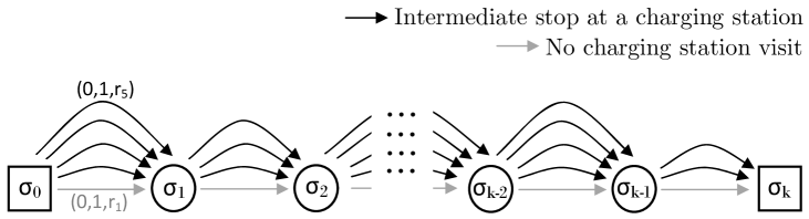
Optimal insertion of charging stations visits. At this point, the algorithm has reconstructed a solution which is feasible in terms of load capacities but usually infeasible in terms of battery capacities. To restore feasibility, it uses a DP algorithm which finds the optimal charging stations positions for each $2^{\text{nd}}$-level route. The problem of inserting charging stations visits in a route $\boldsymbol{\sigma}=(\sigma_{0},\sigma_{1},\dots,\sigma_{K})$ can be reduced to a shortest path problem with resource constraints (SPPRC) in a directed acyclic multigraph $\bar{H}=(\bar{N},\bar{A})$, such that $\bar{N}=\{0\}\cup\{1,\dots,K-1\}\cup\{K\}$. The nodes $0$ and $K$ correspond to depot visits (such that $\sigma_{0}=\sigma_{K}=0$), while the other nodes represent customer visits. Each arc $(i,i+1,r_{k})\in\bar{A}$ corresponds to a non-dominated arc between $\sigma_{i}$ and $\sigma_{i+1}$, with the same characteristics as $(\sigma_{i},\sigma_{i+1},r_{k})\in A^{\prime}$ defined in Section 3 and possible en-route recharging. This multigraph is illustrated in Figure 1.

Figure 1: Illustration of the multigraph $\bar{H}$. Non-dominated choices of charging stations visits are represented by parallel arcs.

Solving this SPPRC can be simply done using Bellman’s algorithm in the topological order $(0,1,\dots,K)$. Using the same notations as in previous sections, the state space graph $\mathscr{\bar{H}}=(\mathscr{\bar{E}},\bar{\Psi})$ is defined as $\mathscr{\bar{E}}=\{(w,i):\forall w,0\leq w\leq L,\forall i\in\bar{N}\}$ and $\bar{\Psi}=\{((w^{\prime},i-1),(w,i))^{p}:\forall(w^{\prime},{i-1}),w^{\prime}\in\Omega(w,\sigma_{i-1},\sigma_{i},p),p=1,\dots,h(\sigma_{i-1},\sigma_{i}),\forall(w,i)\in\mathscr{\bar{E}}\}$. Defining $f(w,i)$ as the minimum cost of a path starting from $0$ and reaching node $i$ with battery consumption $w$, the DP recursion can be expressed as:

$$f(w,i)=\min_{\begin{subarray}{c}1\leq p\leq h(\sigma_{i-1},\sigma_{i})\\ w^{\prime}\in\Omega(w,\sigma_{i-1},\sigma_{i},p)\end{subarray}}\{f(w^{\prime},i-1)+d(\sigma_{i-1},\sigma_{i},p)\},\forall(w,i)\in\mathscr{\bar{E}},\vspace*{0.4cm}$$ (3)

and the initial state is set as $f(0,0)=0$ and $f(w,0)=\infty$ for $w>0$.

In the rare case where no feasible path can be found at the end of the DP recursion, a second execution of the DP algorithm is done, with a minor modification of the label propagation function allowing to use and penalize battery capacity excesses. In this case, any consumption over the battery level $w>L$ is converted into a proportional penalty of $M\times(w-L)$, where $M$ is a large constant. Therefore, the method seeks a route with the smallest penalty in priority, and then the shortest distance. Due to its large impact on the objective, this infeasibility will generally be resolved in the next steps of the method: the local search or the next destroy and repair phase.

5.3 Local search with systematic charging stations relocations

After solution reconstruction, LNS-E2E applies a local search procedure on the $2^{\text{nd}}$-level routes based on 2-opt, 2-opt*, Relocate, Swap and Swap2-1 moves (see, e.g., Vidal et al. 2013, for a detailed description of these neighborhoods). The 2-opt* moves are only tested between routes originated from the same satellite. Moreover, when testing moves that involve routes from different satellites, the algorithm checks that enough capacity is available in the satellites and the associated $1^{\text{st}}$-level routes. The moves are tested in random order and a first-improvement acceptance policy is used, i.e., any move which results in an improvement in terms of cost is directly applied, until no more improvement can be found. Similarly to the granular search by Toth and Vigo (2003), the moves are limited to node pairs $(i,j)$ such that $j$ belongs to one of the $\Gamma$ closest vertices from $i$.

Most modification of the sequence of customer visits or their assignment to vehicles induce some necessary changes in the planning of charging stations visits. Ideally, one would like to apply the labeling algorithm described in Section 5.2 to obtain the exact cost of each move, with an optimal placement of recharging stations in each newly-created route. Such an evaluation would be, however, prohibitive in terms of computational effort. To speed up the method with only a minimal impact on solution quality, we propose some heuristic move filters, which are quite similar in principle to the techniques used by Taillard et al. (1997) for the VRP with soft time windows. We first evaluate each move without the labeling algorithm to obtain an approximation of its impact on the total distance. When doing this calculation, the current locations of the charging stations are unchanged. Any move which is feasible in terms of load capacity and does not deteriorate the total distance by more than $3\%$ is then evaluated exactly in combination with the labeling algorithm, so as to find better charging stations locations which may lead to an improvement. After this exact evaluation, any improving move is applied.

6 Computational Experiments

We conducted extensive experimental analyses with two aims. Firstly, we evaluate the performance of the proposed algorithms for different types of instances, and measure the benefit of integrated routing and recharging-stations planning (Section 6.1). For this analysis, we extend classical 2EVRP instances into E2EVRP instances in order to obtain diverse and challenging datasets and allow possible comparisons with previous algorithms. Secondly, we analyze the impact of two defining features of electric-fueled city-distribution networks: the density of charging stations in a city, and the vehicles’ battery capacities (Section 6.2). For this analysis, we produced a new set of medium-scale instances which simulates a realistic delivery scenario in a metropolitan area, using battery specifications from recent electric vehicles.

The mathematical programming algorithm was coded in Fortran 77, and run on a single thread of a 3.6 GHz Intel i7-4790 CPU with 32GB of RAM. It relies on CPLEX 12.5.1 for the resolution of the linear programs and some integer subproblems. The metaheuristic was coded in Java (JRE 1.8.0–151), and run on a single thread of a 3.4 GHz Intel i7-3770 CPU. All benchmark instances used in this paper are available for download at https://www.univie.ac.at/prolog/research/electric2EVRP and https://w1.cirrelt.ca/~vidalt/en/VRP-resources.html.

6.1 Method performance and benefits of integrated planning

Our benchmark instances for this first analysis are natural extensions of the 2EVRP instances known as Set 2 and 3 by Perboli et al. (2011), Set 5 by Hemmelmayr et al. (2012), and Set 6 by Baldacci et al. (2013). The depot, satellite and customers locations remain unchanged. The new information is associated to the electric vehicles (maximum charging level and energy consumption) and to the charging stations (coordinates).

The selection of charging stations follows the guidelines of Schneider et al. (2014) (instances of the electric vehicle routing problem with time windows and recharging stations (EVRPTWRS)) and Desaulniers et al. (2016). The ratio between charging stations and customers is chosen between $1/10$ and $1/5$. Firstly, every depot and satellite location provides charging abilities vehicles. To pick the remaining locations, we defined a grid of $100\times 100$ candidate locations based upon the range of x- and y-axis coordinates from the existing 2EVRP instances. For each location, we counted the number of customers in “close proximity”, defined as half the average tour length in the best known 2EVRP solution. The more customers one candidate location has in proximity, the more likely it is selected as a charging station. This was achieved by a roulette wheel selection of the remaining charging stations among those 10,000 locations. Finally, all distances are calculated as Euclidean and rounded to the nearest integer value. To reduce the effect of rounding, all x- and y-coordinates from the classical 2EVRP instances have been multiplied by a factor ten. For each instance, the battery capacity has been defined as $L=\max\{0.6\,\gamma_{1},2.0\,\gamma_{2}\}$, where $\gamma_{1}$ represents the average route length of all second-level routes in the best-known 2EVRP solution, and $\gamma_{2}$ is the largest distance of a customer to its closest recharging station. For the sake of simplicity, the energy consumption per distance unit is always set to 1 ($d_{ij}=c_{ij}$). As highlighted in our computational experiments, this approach leads to feasible solutions for all the instances, whereas the best-known 2EVRP solutions are generally not feasible for the corresponding E2EVRP instances.

Parameters calibration. To produce suitable values for the new parameters of the LNS, we used a preliminary meta-calibration based on the covariance matrix adaptation evolution strategy (CMA-ES) of Hansen (2006). During meta-calibration, the parameters are considered to be the decision variables, and the associated objective corresponds to the average solution quality of LNS-E2E over ten runs on a set of training instances. This training set includes six larger-scale instances from Set 5: {100-5-1, 100-5-2b, 100-10-1, 100-10-2b, 200-10-1, 200-10-2b}. Table 1 lists the method parameters, the allowed range for each parameter, and the final values found by the meta-calibration process. These values will be used for the rest of the experiments.

After calibration, we evaluated the proposed mathematical programming algorithm and the metaheuristic on the complete set of benchmark instances. The termination criterion of LNS-E2E has been set to $T_{\textsc{max}}=150$ seconds for the small instances of Sets 2, 3 and 6a, and 900 seconds for the large-scale instances of Set 5.

Table 1: Range of parameters used during meta-calibration, and final values found

	Parameter	Search interval	Final value
$p_{1}$	Related removal (%)	0–100	11
$p_{2}$	Random route removal (%)	0–100	37
$\hat{p}_{3}$	Open all satellites (%)	0–100	12
$\hat{p}_{4}$	Remove single customer routes (%)	0–100	18
$\tau$	Granularity threshold for move evaluations	0–40	25
$i_{max}$	Number of non-improving iterations before restart	0–1000	385

Results on small instances. Table 2 reports the results on the smaller instances of Set 2 and Set 3 with 21 customers. The leftmost group of columns reports the characteristics of the instances: number of customers $n_{c}$, satellites $n_{s}$, trucks $m^{1}$, (electric) second level vehicles $m^{2}$ and charging stations $n_{r}$. The next group of columns shows the performance of the mathematical programming algorithm. The column UB reports the best upper bound at the end of the algorithm, and the solutions marked with an asterisk are proven optimal. The lower bounds obtained at different steps of the exact method are also displayed along with the associated CPU time values, using the same notations as described in Section 4. The next group of columns reports the performance of LNS-E2E: the average (Avg) and best (Best) solution quality over five runs, the average computational time per run (T(s)), and the average time per run needed to reach the final solution of the run (T*(s)). The overall best known solution (BKS) found during all experiments (including calibration and testing) is reported in the rightmost column.

The exact algorithm produced optimal solutions (marked with an asterisk) for all instances except one. A notable improvement is visible when comparing LB2, obtained by repeated resolutions of MDCVRP with side constraints, with LB0 and LB1. The CPU time of the method remains below one minute for 4/12 instances, but can rise up to six hours in other cases, illustrating the difficulty of the E2EVRP, as the presence of the battery capacity constraints significantly increases the time needed for route enumeration. For these instances, the metaheuristic always found the optimal solutions in at least one run out of five. Still, we observe some variance in the results of different independent runs. This is due to the combination of multiple classes of decision variables (two-echelon routing, satellite selection and charging stations selection), which make the problem very intricate and favors the creation of many local minima. The LNS-E2E remains nonetheless accurate, with an average gap of 1.18% from the optimal or best known solutions. The time taken to attain the final solution of the run varies from 2 to 132 seconds, depending on the instance.

Results on medium instances. Table 3 displays the results on the medium instances of Sets 2, 3 and 6a, containing between 32 to 75 customers. The same convention as the previous table is used. For this scale of instances, the mathematical programming algorithm does not generate proven optimal solutions in the allotted time and was stopped after the computation of bound LB1. The average optimality gap between the best solution found by LNS-E2E and the bound LB1, for this group of instances, amounts to 3.57%, demonstrating the good accuracy of both approaches. As usual when comparing exact algorithms with metaheuristics, the difference of CPU time between the two methods becomes more marked for larger instances. For some instances with 75 customers, the time needed to compute LB1 grows as high as 25 hours, whereas the termination of the heuristic is guaranteed after 150 seconds.

Results on large instances, and impact of integrated routing and recharging stations optimization. The larger instances of Set 5 contain 100 or 200 customer visits. To the best of our knowledge, only 3/18 instances have been solved to proven optimality for the classical 2EVRP (without considering electric vehicles and recharging stations). The E2EVRP appears to be even harder to solve, and our exact approach could not produce optimal solutions or good lower bounds in reasonable time. For this set of instances, we therefore concentrate our analysis on the results of the metaheuristic, with the aim of assessing the performance of the algorithm and the impact of an integrated optimization of routing and recharging stations decisions. To that end, we compared four algorithms. The first two algorithms solve the 2EVRP without electric vehicles:

• LNS-2E: the algorithm presented in Breunig et al. (2016) (LNS-2E), which produces the current state-of-the-art results for that problem;

• LNS-E2E $\boldsymbol{\infty}$: the proposed algorithm, in which the range of the electric vehicles is set to $\infty$ to make recharging-stations visits unnecessary.

The two other solution methods are designed for the problem with electric vehicles:

• LNS-2E post: resolution of the classical 2EVRP (disregarding battery constraints) with LNS-2E, followed by a post-optimization using the labeling algorithm to insert charging-stations visits;

• LNS-E2E: the proposed algorithm, with integrated routing and planning of charging stations.

Each method was run until a time limit of 15 minutes, and the same rounding convention (integer distances) have been adopted to allow direct solution comparisons. Table 4 reports the average (Avg) and best (Best) solution quality of each method over ten runs, as well as the average CPU time to reach the final solution of each run (T*(s)). For future reference, the BKS found on Set 5 for the LNS-E2E during preliminary calibration and testing are also listed in the rightmost column.

Firstly, these results highlight the good accuracy of the proposed LNS-E2E, even for the particular case of the 2EVRP without electric vehicles. In comparison with the current state-of-the-art algorithm LNS-2E, better average quality solutions are found on all 200-customer instances, with improvements rising up to 2.41%, while solutions of slightly lower quality are obtained on the 100-customer test cases.

Secondly, we observe the large benefits of an integrated routing and charging stations visits planning. Even when starting with good 2EVRP solutions, a post-ex insertion of charging stations results in solutions of poor quality for the E2EVRP in comparison with the integrated LNS-E2E approach. The average gain related to an integrated optimization in comparison to post-optimization amounts to 3.28%, and can reach as high as 7.93% for instance 100-10-2b. Finally, in terms of computational effort, we observe that the proposed LNS-E2E approach finds solutions in a similar time as LNS-2E, despite the joint optimization of charging stations. This is essentially due to the heuristic move filters described in Section 5.3, allowing to evaluate and discard a large proportion of non-promising local search moves without a call to the labeling algorithm. The next section will study in deeper details the impact of some of these method components.

Table 2: Performance analysis on small instances of Set 2 and 3

	Characteristics					Exact Method										LNS-E2E
Instance	$n_{c}$	$n_{s}$	$m^{1}$	$m^{2}$	$n_{r}$	UB		%LB0	LB0	T${}_{\text{LB0}}$(s)	%LB1	LB1	%LB2	LB2	T${}_{\text{All}}$(s)	Avg	Best	T(s)	T*(s)	BKS
Set2
n22-k4-s6-17	21	2	3	4	4	5229	*	98.23%	5136.3	2.3	98.87%	5169.9	100.00%	5229.00	5.6	5229.0	5229	150	6.1	5229
n22-k4-s8-14	21	2	3	4	4	5094	*	95.95%	4887.6	2.9	95.95%	4887.6	100.00%	5094.00	77.2	5168.4	5094	150	39.8	5094
n22-k4-s9-19	21	2	3	4	4	5236	*	93.95%	4919.1	4.3	93.95%	4919.1	99.62%	5216.26	14.3	5240.2	5236	150	65.3	5236
n22-k4-s10-14	21	2	3	4	4	5561	*	96.99%	5393.6	4.2	96.99%	5393.6	99.64%	5541.15	343.9	5561.0	5561	150	2.0	5561
n22-k4-s11-12	21	2	3	4	4	5793	*	95.92%	5556.6	3.6	95.92%	5556.6	99.24%	5748.74	34.1	5822.0	5793	150	74.8	5793
n22-k4-s12-16	21	2	3	4	4	4125	*	96.96%	3999.5	5.6	97.17%	4008.1	100.00%	4125.00	8.7	4211.4	4125	150	77.5	4125
Average						5173.0		96.33%	4982.1	3.8	96.47%	4989.2	99.75%	5159.02	80.6	5205.3	5173.0	150	44.3	5173.0
Set3
n22-k4-s13-14	21	2	3	4	4	6396	*	95.95%	6137.2	3.8	95.95%	6137.2	99.77%	6381.23	795.2	6406.8	6396	150	15.8	6396
n22-k4-s13-16	21	2	3	4	4	6922	*	97.00%	6714.0	2.1	97.00%	6714.0	99.86%	6912.52	515.1	6954.2	6922	150	31.5	6922
n22-k4-s13-17	21	2	3	4	4	6408	*	93.57%	5996.2	4.1	93.57%	5996.2	98.62%	6319.83	421.1	6408.0	6408	150	35.4	6408
n22-k4-s14-19	21	2	3	4	4	6634		95.27%	6320.4	2.9	95.27%	6320.4	98.60%	6541.32	11995.6	7018.4	6634	150	132.1	6634
n22-k4-s17-19	21	2	3	4	4	6947	*	95.79%	6654.2	4.2	95.79%	6654.2	98.24%	6824.66	20575.4	7094.6	6965	150	72.4	6965
n22-k4-s19-21	21	2	3	4	4	6529	*	96.60%	6307.3	8.2	96.67%	6311.6	99.47%	6494.46	8499.0	6625.2	6529	150	104.9	6529
Average						6639.3		95.70%	6354.9	4.2	95.71%	6355.6	99.09%	6579.00	7133.6	6751.2	6642.3	150	65.4	6642.3

Table 3: Performance analysis on medium-scale instances of Set 2, 3 and 6a

	Characteristics					Lower Bounds							LNS-E2E
Instance	$n_{c}$	$n_{s}$	$m^{1}$	$m^{2}$	$n_{r}$	UB	%LB0	LB0	T${}_{\text{LB0}}$(s)	%LB1	LB1	T${}_{\text{LB1}}$(s)	Avg	Best	BKS	T(s)	T*(s)
Set 2
n33-k4-s1-9	32	2	3	4	5	7617	98.46%	7499.4	73.3	98.46%	7499.4	149.4	7751.0	7617	7617	150	75.3
n33-k4-s2-13	32	2	3	4	5	7925	94.81%	7513.4	44.7	94.81%	7513.4	112.7	8025.0	7925	7925	150	103.3
n33-k4-s3-17	32	2	3	4	5	8090	92.88%	7514.2	69.7	92.88%	7514.2	181.3	8280.2	8090	8090	150	107.0
n33-k4-s4-5	32	2	3	4	5	8870	93.84%	8323.8	79.2	93.84%	8323.8	257.1	8925.2	8870	8870	150	91.0
n33-k4-s7-25	32	2	3	4	5	8318	95.51%	7944.1	77.0	95.74%	7963.3	168.9	8374.8	8318	8318	150	92.7
n33-k4-s14-22	32	2	3	4	5	8621	98.42%	8484.4	218.5	98.42%	8484.4	529.5	8680.4	8621	8621	150	90.2
Average						8240.2	95.65%	7879.9	93.7	95.69%	7883.1	233.1	8339.4	8240.2	8240.2	150	93.3
Set 3
n33-k4-s16-22	32	2	3	4	6	7561	91.60%	6926.2	89.4	91.60%	6926.2	328.4	7656.2	7561	7561	150	94.5
n33-k4-s16-24	32	2	3	4	6	7501	94.77%	7108.5	168.4	94.77%	7108.8	607.1	7520.0	7501	7501	150	102.7
n33-k4-s19-26	32	2	3	4	6	7212	94.42%	6809.5	98.6	94.42%	6809.5	253.4	7223.2	7212	7212	150	47.3
n33-k4-s22-26	32	2	3	4	6	7334	95.81%	7027.0	290.5	96.85%	7103.1	738.5	7498.4	7334	7334	150	131.3
n33-k4-s24-28	32	2	3	4	6	7443	95.40%	7100.5	234.2	96.80%	7204.6	569.9	7371.6	7443	7443	150	116.2
n33-k4-s25-28	32	2	3	4	6	7429	93.68%	6959.7	258.4	93.68%	6959.7	579.8	7490.4	7429	7429	150	108.3
Average						7413.3	94.28%	6988.6	189.9	94.69%	7018.6	512.9	7460.0	7413.3	7413.3	150	100.0
Set 6a
A-n51-4	50	4	2	50	5	7663	95.27%	7300.8	121.9	98.76%	7568.0	762.9	7879.4	7663	7663	150	109.4
A-n51-5	50	5	2	50	6	8268	95.77%	7918.0	98.4	98.16%	8116.0	2783.6	8386.4	8268	8268	150	64.5
A-n51-6	50	6	2	50	7	7795	93.08%	7255.9	117.1	98.18%	7653.4	15723.7	7943.8	7795	7795	150	106.0
A-n76-4	75	4	3	75	7	10599	95.40%	10111.7	214.9	97.23%	10305.4	6463.9	10692.0	10599	10599	150	97.0
A-n76-5	75	5	3	75	7	11178	95.18%	10638.9	175.5	98.17%	10973.6	16406.4	11242.4	11178	11178	150	88.8
A-n76-6	75	6	3	75	7	10156	95.60%	9709.2	242.2	98.92%	10046.1	85538.4	10250.0	10156	10156	150	110.7
B-n51-4	50	4	2	50	5	6589	97.20%	6404.4	163.2	97.96%	6454.8	342.4	6791.2	6589	6589	150	111.6
B-n51-5	50	5	2	50	6	7252	94.73%	6869.8	116.3	95.53%	6928.0	1859.6	7446.4	7252	7240	150	90.8
B-n51-6	50	6	2	50	7	6583	95.02%	6255.0	256.0	97.51%	6419.3	3054.1	6787.6	6583	6583	150	61.4
B-n76-4	75	4	3	75	7	9945	95.99%	9546.7	198.4	98.02%	9748.0	2184.4	9995.8	9945	9943	150	99.5
B-n76-5	75	5	3	75	7	9139	94.70%	8655.1	210.4	98.26%	8980.0	9903.7	9209.2	9139	9139	150	71.9
B-n76-6	75	6	3	75	7	8238	94.44%	7780.1	427.0	97.80%	8056.5	79962.3	8287.6	8238	8238	150	82.4
C-n51-4	50	4	2	50	5	8407	94.57%	7950.2	137.0	95.74%	8048.5	888.4	8596.2	8407	8407	150	80.4
C-n51-5	50	5	2	50	6	8810	94.99%	8368.3	261.1	95.77%	8437.3	1346.5	9276.0	8810	8810	150	82.4
C-n51-6	50	6	2	50	7	8160	93.73%	7648.6	180.3	95.83%	7819.7	7092.7	8390.6	8160	8160	150	72.9
C-n76-4	75	4	3	75	7	12162	94.61%	11506.7	199.0	98.30%	11955.7	3996.1	12381.2	12162	12147	150	99.3
C-n76-5	75	5	3	75	7	13033	92.00%	11990.5	402.2	93.33%	12163.4	38723.3	13247.0	13033	13033	150	79.3
C-n76-6	75	6	3	75	7	11808	93.28%	11014.5	285.0	97.11%	11466.6	93643.4	12129.8	11808	11806	150	92.8
Average						9210.3	94.75%	8718.0	211.4	97.25%	8952.2	20593.1	9385.1	9210.3	9208.6	150	88.9

Table 4: Performance analysis on the large-scale instances of Set 5 – Evaluation of the benefits of an integrated routing and charging-stations optimization

						2EVRP						E2EVRP
	Characteristics					LNS-2E			LNS-E2E $\infty$			LNS-2E post			LNS-E2E
Instance	$n_{c}$	$n_{s}$	$m^{1}$	$m^{2}$	$n_{r}$	Avg	Best	T*(s)	Avg	Best	T*(s)	Avg	Best	T*(s)	Avg	Best	T*(s)	BKS
100-5-1	100	5	5	32	10	15692.6	15640	200.3	15660.9	15639	229.8	16689.9	16593	200.4	16224.6	16167	403.7	16165
100-5-1b	100	5	5	15	10	11124.9	11082	405.9	11208.3	11118	215.7	12802.2	12495	406.0	12070.2	11937	278.4	11937
100-5-2	100	5	5	32	10	10171.0	10157	393.3	10185.1	10157	405.2	11282.4	11189	393.4	10578.0	10578	32.9	10578
100-5-2b	100	5	5	15	10	7814.0	7814	221.5	8032.0	7833	165.4	8833.7	8657	221.6	8426.1	8307	429.4	8307
100-5-3	100	5	5	30	10	10451.0	10451	77.5	10458.1	10451	213.9	10876.7	10863	77.6	10651.4	10651	267.7	10651
100-5-3b	100	5	5	16	10	8283.0	8283	119.5	8287.1	8283	167.7	9341.6	9332	119.6	9068.0	9063	244.8	9018
100-10-1	100	10	5	35	11	11297.0	11247	424.2	11268.2	11247	129.5	11963.8	11942	424.3	11451.8	11409	435.4	11409
100-10-1b	100	10	5	18	11	9243.6	9151	549.3	9257.2	9242	163.3	10374.0	10346	549.4	10194.3	10168	239.5	10168
100-10-2	100	10	5	33	11	10140.8	10100	336.5	10158.0	10127	336.6	10879.0	10829	336.6	10561.5	10525	395.9	10515
100-10-2b	100	10	5	18	11	7825.6	7781	343.4	7965.2	7956	257.5	9558.3	9463	343.5	8800.7	8752	284.0	8621
100-10-3	100	10	5	32	11	10546.9	10503	318.4	10530.1	10490	180.6	11256.4	11164	318.5	10743.6	10730	276.3	10730
100-10-3b	100	10	5	17	11	8646.2	8554	448.7	8683.3	8628	269.2	9503.2	9414	448.8	9209.6	9144	245.2	9144
200-10-1	200	10	5	62	20	15918.6	15615	796.0	15544.6	15453	362.5	16696.7	16426	796.1	16354.8	16016	417.1	16016
200-10-1b	200	10	5	30	20	12310.7	11871	730.7	12076.1	11908	338.5	13510.3	13229	730.8	12975.4	12771	571.8	12768
200-10-2	200	10	5	63	20	13986.3	13669	635.4	13696.4	13577	263.7	14087.1	13971	635.5	14132.9	13860	329.2	13860
200-10-2b	200	10	5	30	20	10089.7	10025	504.2	10257.7	10004	363.0	11099.6	10837	504.3	10833.0	10515	355.4	10495
200-10-3	200	10	5	63	20	18102.1	18000	580.8	17990.0	17925	622.6	18251.8	18167	580.9	18144.4	18094	443.9	18073
200-10-3b	200	10	5	30	20	12088.4	12021	500.4	12001.3	11955	380.0	12711.4	12586	500.5	12515.3	12445	468.0	12441
Average						11318.5	11220.2	421.4	11292.2	11221.8	281.4	12206.6	12083.5	421.5	11829.8	11729.6	339.9	11716.4

Impact of the main LNS components. We conducted additional experiments to measure the contribution of each operator of the LNS-E2E. Starting from the current algorithm (baseline configuration), we deactivated one separate destroy operator listed in Section 5.1, in turn, and measured the solution quality of resulting algorithm. In the specific case of the configuration “No open”, all candidate satellites are made available again (re-opened) at each restart, instead of using this component as a destroy operator. These experiments were conducted on the 18 large instances of Set 5, using 10 independent runs and a time limit $T_{\textsc{max}}=15$ minutes. The solution quality is reported as an average percentage gap from the baseline. Table 5 summarizes the results.

Table 5: Sensitivity analysis on the contribution of each operator.

Baseline	A) No related	B) No route	C) No close	D) No open	E) No single
11829.8	2.70%	2.44%	1.52%	3.10%	1.61%

From these results, we first observe that the “open all satellites” operator (D) is essential for the performance of the method, as it allows to control the frequency of the exploration of different satellite configurations. Without the explicit use of a dedicated operator to re-open satellites, the solutions are 3.10% worse on average. The operator “closes satellite” (C) has a smaller but still very significant impact on the overall solution quality, with a deviation of 1.52% from the baseline when deactivated. Therefore, forcing the elimination of some satellite choices at different phases of the method is essential to evaluate structurally different solutions which would not be attained otherwise by the cheapest insertion repair heuristic.

No related measures the deterioration due to the deactivation of the related nodes destruction operator (A), which destroys specific areas around a seed customer. Analogously, no route measures the performance deterioration when the operator targeting random routes (B) is deactivated, and column no single shows the impact of not using the destruction operator which removes single-customer routes (E). All these operators appear to contribute significantly to the performance of the method, and the deactivation of any of these elements leads to an overall drop of method performance.

We finally tested a version of the method without a restart process after each $i_{max}$ iterations without improvement. In this configuration, the loop of Algorithm 1, Line 4–8 is executed until reaching a maximum time of $T_{\textsc{max}}$. We observed a deterioration of solution quality of $1.90\%$ with respect to the baseline, demonstrating again the importance of diversification components, in this case the restarts mechanism, for the E2E-VRP.

6.2 Sensitivity analysis – Density of charging stations and battery capacity

Our second set of experiments focuses on the impact of two defining features of battery-powered distribution networks: the density of the charging stations, and the range of the vehicles. To that extent, we created two additional sets of instances with $n_{c}=50$ customers and $n_{s}=4$ satellites each, approximating as closely as possible real delivery conditions in a metropolitan area while pertaining to the E2EVRPs class. Set 7 contains 10 groups of 20 instances with a number of charging stations $n_{r}\in\{2,3,5,10,15,20,25,30,40,50\}$ (in addition to the satellites) and a battery capacity $L=1000$, whereas Set 8 contains 10 groups of 20 instances with $n_{r}=20$ charging stations and a battery capacity $L\in\{800,900,1000,\dots,1700\}$. When varying the number of charging stations or the battery capacity, all other instance characteristics (satellite locations, customers locations and demands as well as the existing charging stations locations) are kept identical.

In each instance, 40 customers have been located randomly (with uniform probability) in an ellipse $X_{1}$ centered in (1000,500), with x-axis of dimension 800 and y-axis of dimension 400, and 10 additional customers have been located randomly in an ellipse $X_{2}$ with the same center, an x-axis of dimension 1000 and y-axis of dimension 500. The locations of the satellites are picked randomly in the area formed by $X_{2}-X_{1}$, and the depot is fixed in position (300,0). Moreover, 80% of the charging stations are randomly located in $X_{1}$, and $20\%$ in $X_{2}$. The demand quantity of each customer is randomly selected in [1,25]. Six $1^{\text{st}}$-level vehicles with capacity $Q_{1}=250$ are available, and ten $2^{\text{nd}}$-level electric vehicle with capacity $Q_{2}=125$ are available at each satellite.

Considering that one distance unit in each instance corresponds to 0.1km on a map, the area considered for the location of customers and charging stations covers 15708 km², a size similar in magnitude with the metropolitan area of Paris. We set a baseline of $L=1000$ for the battery capacity, equivalent to a range of 100km. This value matches the specifications of the Renault Kangoo Zoe and Nissan Leaf 2015/2016 minus a safety range of 30km. Varying this parameter allows to evaluate the impact of the battery capacity.

Figure 2 depicts the evolution of the operational costs as a function of the number of charging stations $n_{r}$, and Figure 3 shows the impact of the battery capacity $L$. The results are expressed as percentage gaps between the cost of the LNS-E2E solution with and without battery restrictions (i.e. percentage detour miles due to recharging), and averaged over all 20 instances of each class. The average number of visits to charging stations in the solutions is also represented on each graph.

Figure 2: Impact of the number of available charging stations on the detour costs due to recharging and the number of visits to stations.

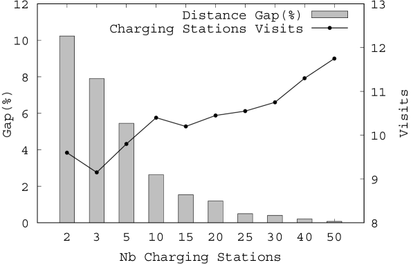
These experiments highlight the significant impact of the charging stations density and vehicles batteries capacities in the instances under study. As the number of charging stations grows, the detour costs due to recharging stations visits rapidly decreases: e.g., from 5.45% in average when $n_{r}=5$ to 1.53% when $n_{r}=15$. Conducting a power-law regression of the form $f(n_{r})=\alpha/n_{r}^{\beta}$ (least-squares regression of an affine function on the log-log graph), the extra detours due to recharging diminish proportionally to $1/\rho^{1.24}$. In these conditions, doubling the number of charging stations allows to reduce extra recharging costs by approximately 58%.

Interestingly, the number of visits to charging stations slightly increases with $n_{r}$: from 9.5 in average when $n_{r}=2$ to 11.75 when $n_{r}=50$. Indeed, when the recharging station network is sparse, most detour options to recharging stations involve significant extra costs, and the vehicle routing algorithm tends to reduce to a strict minimum the number of such detours. In contrast, in the presence of a dense recharging stations network, the solutions converge more closely towards the 2E-VRP cost (disregarding battery constraints) as there are always multiple options of charging stations on the way.

Figure 3: Impact of the vehicle range (i.e., battery capacity) on the detour costs due to recharging and the number of visits to stations.

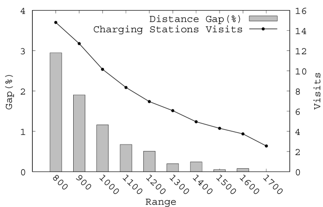
The vehicles’ range (i.e., battery capacity), has an even larger impact (see Figure 3). For most of the considered instances, a range below $700$ distance units ($=$ 70km) would lead to an infeasible problem, as it becomes impossible to travel between some pairs of customers and find adequate recharging locations en-route. Therefore, adequate battery technology is a key factor for the viability of battery-powered delivery networks. The extra costs due to recharging and number of visits to recharging stations tend to be high when considering vehicles’ ranges close to the feasible limit ($L=800$). These values then rapidly decrease to become close to zero when the range $L$ exceeds $1500$ (i.e., $150$km), a value which may be soon attained by lightweight electric trucks. Once this regime is attained, the battery capacity becomes sufficient to do most tours without en-route recharging visits. Still, manufacturing the current best-performing batteries on a global scale requires a large supply of minerals (e.g., nickel and cobalt) which are only accessible in limited quantities in the environment. As illustrated in Figure 2, the development of good fast-charging infrastructures is another strategic development path to obtain operational efficiency, which may turn out, in the long run, to be more sustainable and economical than a race towards heavier and more robust batteries.

7 Conclusions

In this paper, we have formulated the E2EVRP, an extension of the 2EVRP involving electric vehicles for second-echelon deliveries, battery capacity constraints, and possible visits to charging stations, and used it as a prototypical problem for the study of multi-echelon battery-powered supply chains. We introduced an efficient exact algorithm, based on the enumeration of candidate solutions for the first echelon and on bounding functions and route enumeration for the second echelon, along with a problem-tailored large neighborhood search metaheuristic (LNS-E2E). A comparison of the solutions found by the LNS-E2E with lower bounds and optimal solutions produced by the mathematical programming algorithm demonstrates the excellent performance of both algorithms. In particular, all known optimal solutions for small instances were retrieved by the LNS-E2E, and an average optimality gap of 3.57% between the best known upper and lower bounds was obtained on medium-scale instances. The metaheuristic was also evaluated on the classical 2EVRP (without electric vehicles), producing new state-of-the-art solutions on large-scale instances with 200 customers. Finally, thanks to the use of efficient heuristic move filters in the local search and labeling algorithms, the computational effort of LNS-E2E remains comparable with that of previous metaheuristics for the classical 2EVRP.

Beyond the usefulness of these optimization algorithms for the operational planning of electric fleets, this paper brought new managerial insights related to the incorporation of electric vehicles into two-echelon delivery networks and to the recharging-stations infrastructure required for an efficient supply chain. For this additional study, we created 400 additional test instances simulating typical requests patterns and delivery infrastructures in a metropolitan area with varying density of charging stations vehicles’ battery capacities. We observed that the detour miles due to recharging decrease in $\mathcal{O}(1/\rho^{x})$ with $x\approx 5/4$ as a function of the number of charging stations. Moreover, the range of the electric vehicles has an even bigger impact: an increase of battery capacity to a range of 150km helps performing the majority of suburban delivery tours without need for en-route recharging, but a battery capacity below 80km render electric deliveries unviable in our setting. Between these two extremes, the extra costs due to recharging quickly decrease as a function of the battery capacity.

The future research perspectives are multiple. Firstly, we recommend to pursue the study of exact methods and metaheuristics for multi-echelon electric VRPs. These optimization problems involve a large number of decision classes, related to satellite choices, recharging stations choices, and vehicle routing at two levels, posing a formidable challenge for exact and heuristic algorithms alike. With the rapid development of battery-powered vehicles and green supply chains, efficient algorithms for large scale problems are critically needed, but the current methods still need to be improved in terms of accuracy, scalability, and generality, e.g., considering possible extensions to multi-echelon electric delivery schemes arising in city logistics (Cattaruzza et al. 2017), other vehicle routing attributes (Vidal et al. 2013) and stochastic settings.

Secondly, our sensitivity analyses on electric vehicles characteristics and other strategic decisions (number and placement of charging stations) could be extended further. One limitation of the current study relates to the placement of the charging stations, which is randomized in a fixed area. However, during urban planning, recharging stations are placed in strategical locations to meet the needs of the population, or based on competitive location approaches. Solving this strategic location optimization problem may be necessary for a more accurate sensitivity analysis. Yet, it is an intricate problem, which can be viewed as a variant of location routing problems (Schiffer and Walther 2017a, b), or modeled as a bilevel optimization problem and congestion game (Xiong et al. 2015). To this date, the optimization of charging stations locations has never been considered in the context of a multi-echelon delivery network, forming a promising research avenue.

Bibliography

- Baldacci and Mingozzi (2009) R. Baldacci and A. Mingozzi. A unified exact method for solving different classes of vehicle routing problems. Mathematical Programming Ser. A, 120(2):347–380, 2009.
- Baldacci et al. (2011) R. Baldacci, A. Mingozzi, and R. Roberti. New route relaxation and pricing strategies for the vehicle routing problem. Operations Research, 59(5):1269–1283, 2011.
- Baldacci et al. (2013) R. Baldacci, A. Mingozzi, R. Roberti, and R. Wolfler Calvo. An exact algorithm for the two-echelon capacitated vehicle routing problem. Operations Research, 61(2):298–314, 2013.
- Breunig et al. (2016) U. Breunig, V. Schmid, R. Hartl, and T. Vidal. A large neighbourhood based heuristic for two-echelon routing problems. Computers & Operations Research, 76:208–225, 2016.
- Cattaruzza et al. (2017) D. Cattaruzza, N. Absi, D. Feillet, and J. González-Feliu. Vehicle routing problems for city logistics. EURO Journal on Transportation and Logistics, 6(1):51–79, 2017.
- Christofides et al. (1981) N. Christofides, A. Mingozzi, and P. Toth. Exact algorithms for the vehicle routing problem based on spanning tree and shortest path relaxation. Mathematical Programming, 10:255–280, 1981.
- Conrad and Figliozzi (2011) R. G. Conrad and M. A. Figliozzi. The recharging vehicle routing problem. In T. Doolen and E. V. Aken, editors, Proceedings of the 2011 Industrial Engineering Research Conference, pages 1–8, 2011.
- Cuda et al. (2015) R. Cuda, G. Guastaroba, and M. G. Speranza. A survey on two-echelon routing problems. Computers & Operations Research, 55:185–199, 2015.
- Desaulniers et al. (2016) G. Desaulniers, F. Errico, S. Irnich, and M. Schneider. Exact algorithms for electric vehicle-routing problems with time windows. Operations Research, 64(6):1388–1405, 2016.
- Erdogan and Miller-Hooks (2012) S. Erdogan and E. Miller-Hooks. A green vehicle routing problem. Transportation Research Part E: Logistics and Transportation Review, 48(1):100–114, 2012.
- EV World (2008) EV World. Beijing readies electric buses for summer olympics. http://www.evworld.com/news.cfm?newsid=18730 (accessed Oct 13, 2018), 2008.
- Felipe et al. (2014) A. Felipe, M. T. Ortuno, G. Righini, and G. Tirado. A heuristic approach for the green vehicle routing problem with multiple technologies and partial recharges. Transportation Research Part E: Logistics and Transportation Review, 71:111–128, 2014.
- Foltyński (2014) M. Foltyński. Electric fleets in urban logistics. Procedia – Social and Behavioral Sciences, 151:48–59, 2014.
- Goeke and Schneider (2015) D. Goeke and M. Schneider. Routing a mixed fleet of electric and conventional vehicles. European Journal of Operational Research, 245(1):81–99, 2015.
- Gonzalez-Feliu et al. (2008) J. Gonzalez-Feliu, G. Perboli, R. Tadei, and D. Vigo. The two-echelon capacitated vehicle routing problem. Technical report, DEIS OR.INGCE 2007/2(R), University of Bologna, Bologna, Italy, 2008.
- Hansen (2006) N. Hansen. The CMA evolution strategy: a comparing review. In J. Lozano, P. Larranaga, I. Inza, and E. Bengoetxea, editors, Towards a new evolutionary computation. Advances on estimation of distribution algorithms, pages 75–102. Springer Berlin Heidelberg, 2006.
- Hemmelmayr et al. (2012) V. C. Hemmelmayr, J.-F. Cordeau, and T. G. Crainic. An adaptive large neighborhood search heuristic for two-echelon vehicle routing problems arising in city logistics. Computers & Operations Research, 39(12):3215–3228, 2012.
- Hiermann et al. (2016) G. Hiermann, J. Puchinger, S. Ropke, and R. F. Hartl. The electric fleet size and mix vehicle routing problem with time windows and recharging stations. European Journal of Operational Research, 252(3):995–1018, 2016.
- Hiermann et al. (2019) G. Hiermann, R. Hartl, J. Puchinger, and T. Vidal. Routing a mix of conventional, plug-in hybrid, and electric vehicles. European Journal of Operational Research, 272(1):235–248, 2019.
- Hof et al. (2017) J. Hof, M. Schneider, and D. Goeke. Solving the battery swap station location-routing problem with capacitated electric vehicles using an AVNS algorithm for vehicle-routing problems with intermediate stops. Transportation Research Part B: Methodological, 97:102–112, 2017.
- JD.com (2018) JD.com. Urban truck routing and scheduling contest page. http://jdata.joybuy.com/en/html/detail.html?id=5 (accessed Oct 13, 2018), 2018.
- Jepsen et al. (2012) M. Jepsen, S. Spoorendonk, and S. Ropke. A branch-and-cut algorithm for the symmetric two-echelon capacitated vehicle routing problem. Transportation Science, 47(1):23–37, 2012.
- John (2017) J. John. JD.com CEO sets february 2018 target to change its fleet of delivery vans in beijing to electric. https://www.gizmochina.com/2017/12/13/jd-com-ceo-sets-february-2018-targetchange-fleet-delivery-vans-beijing-electric/ (accessed Oct 13, 2018), 2017.
- Keskin and Çatay (2018) M. Keskin and B. Çatay. A matheuristic method for the electric vehicle routing problem with time windows and fast chargers. Technical report, Sabanci University, Istanbul, Turkey, 2018.
- Keskin and Çatay (2016) M. Keskin and B. Çatay. Partial recharge strategies for the electric vehicle routing problem with time windows. Transportation Research Part C: Emerging Technologies, 65:111–127, 2016.
- Montoya (2016) J.-A. Montoya. Electric vehicle routing problems: models and solution approaches. PhD thesis, Université d’Angers, 2016.
- Pelletier et al. (2016) S. Pelletier, O. Jabali, and G. Laporte. 50th anniversary invited article – goods distribution with electric vehicles: review and research perspectives. Transportation Science, 50(1):3–22, 2016.
- Perboli and Rosano (2018) G. Perboli and M. Rosano. A decision support system for optimizing the last-mile by mixing traditional and green logistics. In C. Temponi and N. Vandaele, editors, Information Systems, Logistics, and Supply Chain, pages 28–46. Springer International Publishing, 2018.
- Perboli et al. (2010) G. Perboli, R. Tadei, and F. Masoero. New families of valid inequalities for the two-echelon vehicle routing problem. Electronic Notes in Discrete Mathematics, 36(Supplement C):639–646, 2010.
- Perboli et al. (2011) G. Perboli, R. Tadei, and D. Vigo. The two-echelon capacitated vehicle routing problem: models and math-based heuristics. Transportation Science, 45(3):364–380, 2011.
- Perboli et al. (2018a) G. Perboli, M. Rosano, M. Saint-Guillain, and P. Rizzo. Simulation -optimisation framework for City Logistics: an application on multimodal last-mile delivery. IET Intelligent Transport Systems, 12(4):262–269, 2018a.
- Perboli et al. (2018b) G. Perboli, R. Tadei, and E. Fadda. New Valid Inequalities for the Two-Echelon Capacitated Vehicle Routing Problem. Electronic Notes in Discrete Mathematics, 64:75–84, 2018b.
- Pisinger and Ropke (2007) D. Pisinger and S. Ropke. A general heuristic for vehicle routing problems. Computers & Operations Research, 34(8):2403–2435, 2007.
- Poikonen et al. (2017) S. Poikonen, X. Wang, and B. Golden. The vehicle routing problem with drones: Extended models and connections. Networks, 70(1):34–43, 2017.
- Santos et al. (2015) F. A. Santos, G. R. Mateus, and A. Salles da Cunha. A branch-and-cut-and-price algorithm for the two-echelon capacitated vehicle routing problem. Transportation Science, 49(2):355–368, May 2015.
- Schiffer and Walther (2017a) M. Schiffer and G. Walther. The electric location routing problem with time windows and partial recharging. European Journal of Operational Research, 260(3):995–1013, 2017a.
- Schiffer and Walther (2017b) M. Schiffer and G. Walther. An adaptive large neighborhood search for the location-routing problem with intra-route facilities. Transportation Science, Articles in Advance, 2017b.
- Schiffer et al. (2016) M. Schiffer, S. Stütz, and G. Walther. Are ECVs breaking even? - Competitiveness of electric commercial vehicles in medium-duty logistics networks. Technical report, OM-02, 2016.
- Schiffer et al. (2018) M. Schiffer, M. Schneider, G. Walther, and G. Laporte. Vehicle routing and location-routing with intermediate stops: A review. Transportation Science, 2018. To appear.
- Schneider et al. (2014) M. Schneider, A. Stenger, and D. Goeke. The electric vehicle routing problem with time windows and recharging stations. Transportation Science, 48(4):500–520, 2014.
- Shaw (1998) P. Shaw. Using constraint programming and local search methods to solve vehicle routing problems. In M. Maher and J.-F. Puget, editors, Principles and Practice of Constraint Programming, volume 1520 of Lecture Notes in Computer Science, pages 417–431. Springer Berlin Heidelberg, 1998.
- Taillard et al. (1997) E. Taillard, P. Badeau, M. Gendreau, F. Guertin, and J.-Y. Potvin. A tabu search heuristic for the vehicle routing problem with soft time windows. Transportation Science, 31(2):170–186, 1997.
- Toth and Vigo (2003) P. Toth and D. Vigo. The granular tabu search and its application to the vehicle-routing problem. INFORMS Journal on Computing, 15(4):333–346, 2003.
- Vidal et al. (2013) T. Vidal, T. Crainic, M. Gendreau, and C. Prins. Heuristics for multi-attribute vehicle routing problems: A survey and synthesis. European Journal of Operational Research, 231(1):1–21, 2013.
- Wang et al. (2017a) K. Wang, S. Lan, and Y. Zhao. A genetic-algorithm-based approach to the two-echelon capacitated vehicle routing problem with stochastic demands in logistics service. Journal of the Operational Research Society, pages 1–13, 2017a.
- Wang et al. (2017b) X. Wang, S. Poikonen, and B. Golden. The vehicle routing problem with drones: Several worst-case results. Optimization Letters, 11(4):679–697, 2017b.
- Wang et al. (2017c) Y. Wang, Y. Huang, J. Xu, and N. Barclay. Optimal recharging scheduling for urban electric buses: A case study in Davis. Transportation Research Part E: Logistics and Transportation Review, 100:115–132, 2017c.
- Wr. Linien (2013) Wr. Linien. Wiener Linien mit Staatspreis Mobilität ausgezeichnet. https://www.wien.gv.at/presse/2013/09/13/wiener-linien-mit-staatspreis-mobilitaet-ausgezeichnet, in German, (accessed Oct 13, 2018), 2013.
- Xiong et al. (2015) Y. Xiong, J. Gan, B. An, C. Miao, and A. Bazzan. Optimal electric vehicle charging station placement. In Proceedings of the 24th International Conference on Artificial Intelligence, IJCAI’15, pages 2662–2668, 2015.
- Yang and Sun (2015) J. Yang and H. Sun. Battery swap station location-routing problem with capacitated electric vehicles. Computers & Operations Research, 55:217–232, 2015.
- Zeng et al. (2014) Z.-Y. Zeng, W.-S. Xu, Z.-Y. Xu, and W.-H. Shao. A hybrid GRASP+VND heuristic for the two-echelon vehicle routing problem arising in city logistics. Mathematical Problems in Engineering, 2014:1–11, 2014.