Gravitational lensing by eigenvalue distributions of random matrix models

Abstract

We propose to use eigenvalue densities of unitary random matrix ensembles as mass distributions in gravitational lensing. The corresponding lens equations reduce to algebraic equations in the complex plane which can be treated analytically. We prove that these models can be applied to describe lensing by systems of edge-on galaxies. We illustrate our analysis with the Gaussian and the quartic unitary matrix ensembles.

1 Introduction

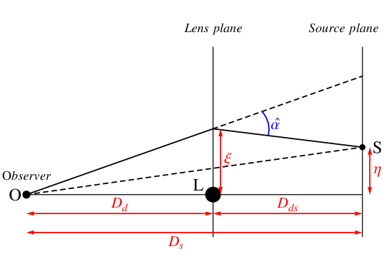
The trajectory of light from distant sources is perturbed by foreground distributions of matter such as galaxies, groups and clusters. This phenomenon is called gravitational lensing and it has important applications in cosmology [1, 2]. The deflection angle $\widehat{\alpha}$ of a light ray passing at a minimum distance $\xi$ (impact parameter) of a point-like mass $M$ is given by the Einstein’s formula

$$\widehat{\alpha}=\frac{4GM}{\xi},$$ (1)

see e.g. Chapter 4 of Ref. [1] and Figure 1, where $G$ is the constant of gravity. In general, the deflection angle is defined as the vector $\widehat{\boldsymbol{\alpha}}={\bf e}_{i}-{\bf e}_{f}$ where ${\bf e}_{i}$ and ${\bf e}_{f}$ are the initial and final unit tangent vectors to the light ray trajectory from the source to the observer, respectively. For thin lenses with continuous mass distributions and weak gravitational fields, the deflection angle is the sum of the deflections due to each mass element of the lens. Thus $\widehat{\boldsymbol{\alpha}}(\boldsymbol{\xi})$ is a function $\widehat{\boldsymbol{\alpha}}(\boldsymbol{\xi})$ of the impact vector $\boldsymbol{\xi}$ in the lens plane [1],

$$\widehat{\boldsymbol{\alpha}}(\boldsymbol{\xi})=4G\int_{\mathbb{R}^{2}}\frac{\boldsymbol{\xi}-\boldsymbol{\xi}^{\prime}}{|\boldsymbol{\xi}-\boldsymbol{\xi}^{\prime}|^{2}}\Sigma(\boldsymbol{\xi}^{\prime})d^{2}\boldsymbol{\xi}^{\prime},$$ (2)

where $\Sigma(\boldsymbol{\xi})$ is the surface mass density obtained by projecting the volume mass distribution of the deflector onto the lens plane. Moreover, there is a geometrical relation (see Chapter 4 of Ref. [1]) between the source position $\boldsymbol{\eta}$ and the impact vector $\boldsymbol{\xi}$ of the ray in the lens plane

$$\boldsymbol{\eta}=\frac{D_{s}}{D_{d}}\boldsymbol{\xi}-D_{ds}\widehat{\boldsymbol{\alpha}}(\boldsymbol{\xi}),$$ (3)

where $D_{s}$, $D_{d}$ and $D_{ds}$ are the distances from the observer to the source plane, from the observer to the lens, and from the lens to the source plane, respectively (see the diagram of Figure 1). In effect, we have a correspondence between vectors $\boldsymbol{\xi}$ in the lens plane and vectors $\boldsymbol{\eta}$ in the source plane. The problem of gravitational lensing is the inversion of this correspondence, i.e. to determine the image positions $\boldsymbol{\xi}$ for a given source position $\boldsymbol{\eta}$. Images $\boldsymbol{\xi}$ outside (inside) the mass distribution $\Sigma(\boldsymbol{\xi})$ are referred to as bright (dim) images.

Figure 1: A lensing system with a source $S$, a lens $L$ and an observer $O$. The lens deflects a light ray emanating from the source by an angle $\widehat{\alpha}$.

The computation of the image positions for a given source is a difficult problem [5], which in general can be solved only numerically. Even the two point-mass lens [6] is already very complicated to study analytically. Hence, it is interesting to find lensing systems allowing partial or total analytic treatment. Among the possible candidates are the mass distributions defined by measures with minimal support (consisting of a finite set of isolated points or/and a finite number of compact analytic curves). Measures of this type arise in the study of families of measures producing the same external gravitational potential and are known as mother bodies in geophysics [7]. They have been mathematically defined in several forms, see e.g. [8, 9, 10]. The concrete notion of mother body measure used in this paper is given in the next section.

The present work is devoted to lensing models in which the mass distributions are determined by the eigenvalue densities of unitary random matrix ensembles in the limit of large matrix dimension [11, 12, 13]. These mass distributions are non-trivial examples of mother bodies supported on a finite number of real intervals (cuts). The corresponding lens equations turn out to reduce to algebraic equations and exhibit interesting classes of explicit analytic solutions. In particular, we propose to apply these models to describe gravitational lensing by disk galaxies seen edge-on (see [14] for a catalog of this type of galaxies). Thus an $n$-cut eigenvalue density describes a lensing system of $n$ coplanar edge-on galaxies. Consequently, phase transitions of eigenvalue distributions in which the number of cuts changes [13, 15, 16] represent splitting-merging processes of edge-on galaxies. Moreover, due to their mother body character, the eigenvalue distributions can be also applied to determine the bright images of more general mass distributions. We illustrate our analysis with two well-known random matrix models: the Gaussian and the quartic models. We study their eigenvalue distributions as mother bodies supported on elliptic domains and formulate their associated lensing models by edge-on galaxies. We consider the corresponding lens equations and derive explicit expressions for wide classes of dim and bright images. We also include some exact calculations of time delays.

The layout of this paper is as follows. Section 2 concentrates on the main properties of the eigenvalue distributions of unitary ensembles of random matrix models and formulates the corresponding lens models. Then we discuss these distributions as mother body measures and edge-on disk galaxies. Sections 3 and 4 contain our main explicit results. Section 3 is devoted to the lens model of the Gaussian eigenvalue distribution and Section 4 deals with the lens model corresponding to the unitary ensemble of random matrices with a quartic potential. After some concluding remarks on several open questions, the paper ends with one appendix where it is proved that the Gaussian and the quartic models are mother bodies on elliptic domains.

2 Gravitational lensing by eigenvalue distributions

2.1 Complex formulation of the lens equation

It is convenient to write the lens equation (3) in dimensionless form. Thus, we introduce dimensionless vectors $\boldsymbol{x}=\boldsymbol{\xi}/\xi_{0}$ and $\boldsymbol{y}=\boldsymbol{\eta}/\eta_{0}$, where $\xi_{0}$ is a fixed length scale (whose choice depends on the particular problem studied) and $\eta_{0}=\xi_{0}D_{s}/D_{d}$. Then we have

$$\boldsymbol{y}=\boldsymbol{x}-\int_{\mathbb{R}^{2}}\frac{\boldsymbol{x}-\boldsymbol{x}^{\prime}}{|\boldsymbol{x}-\boldsymbol{x}^{\prime}|^{2}}\kappa(\boldsymbol{x}^{\prime})d^{2}\boldsymbol{x}^{\prime},$$ (4)

where $\kappa(\boldsymbol{x})=4GD_{d}D_{ds}\Sigma(\xi_{0}\boldsymbol{x})/D_{s}$. If we now represent the two-dimensional vectors $\boldsymbol{x}$ and $\boldsymbol{y}$ by complex numbers $z$, $w$, and complex conjugate the resulting equation, we obtain [4]

$$\overline{w}=\overline{z}-\omega(z),$$ (5)

where $\omega(z)$ is the Cauchy transform (in the principal value sense)

$$\omega(z)=\int_{\mathbb{C}}\frac{d\mu(\zeta)}{z-\zeta},$$ (6)

of the mass distribution $d\mu=\kappa(\zeta)d^{2}\zeta$. In order to avoid the singularity at $\zeta=z$ the integral (6) is assumed to be defined in the principal value sense, (i.e. we integrate on the domain $|\zeta-z|>\epsilon$ of the $\zeta$ plane and then we take the limit as $\epsilon\rightarrow 0$). Equation (5) provides a quite useful complex formulation of the lens equation which allows us to apply various tools of complex analysis.

2.2 Eigenvalue distributions of matrix models

We consider random matrix models of $N\times N$ Hermitian matrices $M$ with Boltzmann weights of the form $\exp(-2NV(M))$ where the potential function $V(x)$ is a real polynomial function of even degree $V(x)=\sum_{i=1}^{2p}t_{i}x^{i}$ with $t_{2p}>0$ (unitary ensembles) [11, 12, 13]. The associated unit normalized eigenvalue density in the limit $N\rightarrow\infty$ is supported on a finite union of disjoint real intervals

$$\Gamma=\cup_{i=1}^{n}[a_{i},b_{i}],$$ (7)

with

$$\int_{\Gamma}\rho(x)\,dx=1,$$ (8)

and is of the form

$$\rho(x)=p(x)\sqrt{\prod_{i=1}^{n}(x-a_{i})(b_{i}-x)},$$ (9)

for a given polynomial $p(x)$.

The density $\rho(x)$ determines a mass distribution $d\mu_{e}=\rho(x)dx$ with the one-dimensional support $\Gamma$. From the point of view of the applications to gravitational lensing the main property of $\mu_{e}(z)$ is that its Cauchy transform

$$\omega_{e}(z)=\int_{\Gamma}\frac{\rho(x)dx}{z-x},$$ (10)

satisfies a quadratic equation [12, 13]

$$\Big{(}\omega_{e}(z)-V^{\prime}(z)\Big{)}^{2}=P(z),$$ (11)

where $P(z)$ is a polynomial such that ${\rm deg}\,P=2\,{\rm deg}\,V-2$. As a consequence the function $\omega_{e}(z)$ can be explicitly calculated in terms of $V$ and $P$. Indeed, from (11) and taking into account that $\omega_{e}(z)\sim 1/z$ as $z\rightarrow\infty$ we have that outside $\Gamma$

$$\omega_{e}(z)=V^{\prime}(z)-\sqrt{P(z)},\quad z\in\mathbb{C}\setminus\Gamma,$$ (12)

where the branch of $\sqrt{P(z)}$ is determined by the condition

$$V^{\prime}(z)-\sqrt{P(z)}=\frac{1}{z}+\mathcal{O}(1/z^{2}),\quad z\rightarrow\infty.$$ (13)

The expression of $\omega_{e}(z)$ on $\Gamma$ can be derived from the boundary values of $\omega_{e}(z)$ on both sides of $\Gamma$

$$\omega_{e\pm}(x)=\lim_{\epsilon\rightarrow+0}\omega_{e}(x+\pm i\epsilon),\quad x\in\Gamma.$$ (14)

Thus, since the integral (10) is defined in the principal value sense, the Sokhotsky-Plemelj formulas [17, 18]

$$\omega_{e\pm}(x)=\omega_{e}(x)\mp i\pi\rho(x),\quad x\in\Gamma,$$ (15)

imply that

$$\omega_{e}(x)=\frac{1}{2}\Big{(}\omega_{e+}(x)+\omega_{e-}(x)\Big{)},\quad x\in\Gamma.$$ (16)

Hence, as $\sqrt{P(z)}$ has opposite boundary values on both sides of $\Gamma$, from (12) and (16) we get

$$\omega_{e}(x)=V^{\prime}(x),\quad x\in\Gamma.$$ (17)

Therefore (12) and (17) provide an explicit characterization of the Cauchy transform $\omega_{e}(z)$ on the whole complex plane.

Similarly, it follows from (12) and (15) that the eigenvalue density $\rho(x)$ is given by

$$\rho(x)=\frac{1}{\pi}\Big{|}\sqrt{P(x)}\Big{|},\quad x\in\Gamma.$$ (18)

Furthermore, it can be proved [12, 13] that $\rho(x)$ represents an equilibrium configuration in the sense that the total potential function

$${\rm Re}V(z)+U(z),\quad z\in\mathbb{C},$$ (19)

where $U(z)$ denotes the logarithmic potential

$$U(z)=-\int_{\Gamma}\ln|z-x|\,\rho(x)dx,\quad z\in\mathbb{C},$$ (20)

is constant on $\Gamma$

$$V(x)+U(x)=U_{0},\quad x\in\Gamma.$$ (21)

2.3 Lensing by eigenvalue distributions

Henceforth we consider mass distributions of the form

$$\mu=m\,\mu_{e},$$ (22)

where the parameter $m>0$ represents the total mass of $\mu$. From (12) and (17) we have that these distributions have an explicit Cauchy transform $\omega=m\omega_{e}$ and the lens equation is determined by the functions $V(z)$ and $P(z)$ as follows

$$\left\{\begin{array}[]{ll}w=x-mV^{\prime}(x),\quad\mbox{if $x\in\Gamma$ },\\ \\ \overline{w}=\overline{z}-mV^{\prime}(z)+m\sqrt{P(z)},\quad\mbox{if $z\in\mathbb{C}\setminus\Gamma$.}\end{array}\right.$$ (23)

An important parameter in gravitational lensing is the time it takes the light to travel from the source to the observer [1]. In Eq.(5.45) of Ref. [1] it is proved that up to an additive constant the excess travel time for a light ray with source $w$ crossing the lens plane at $z$, relative to an undeflected ray is proportional to

$$\tau(z)=\frac{1}{2}|z-w|^{2}+m\,U(z),$$ (24)

where $U(z)$ is the logarithmic potential determined by the mass distribution $\mu_{e}$. We will henceforth refer to $\tau(z)$ as the time delay. In particular, from (21) and (24) we have that given a dim image $z=x\in\Gamma$

$$\tau(x)=\frac{1}{2}|x-w|^{2}+m\Big{(}U_{0}-V(x)\Big{)},\quad x\in\Gamma.$$ (25)

Hence (25) implies that the relative time delay between two dim images for a given source $w$ is proportional to

$$\tau(x_{2})-\tau(x_{1})=\frac{1}{2}\Big{(}|x_{2}-w|^{2}-|x_{1}-w|^{2}\Big{)}+m\Big{(}V(x_{1})-V(x_{2})\Big{)}.$$ (26)

2.4 Mother bodies

Let $D$ be a bounded domain of the complex plane and $\mu_{D}$ a measure with support $\overline{D}$. We may think of the pair $(D,\mu_{D})$ as a planar body with mass distribution $\mu_{D}$. Then another measure $\mu$ is said to be a mother body for $(D,\mu_{D})$ if [8, 19]:

1. The support of $\mu$ is a finite set of curve segments or/and points contained in $\overline{D}$ such that each connected component of $\mathbb{C}\setminus{\rm supp}\mu$ does not disconnect any part of $D$ from the complement of $D$.

2. The gravitational potentials of $\mu$ and $\mu_{D}$ coincide on $\mathbb{C}\setminus\overline{D}$.

Since the Cauchy transform and the logarithmic potential of a measure satisfy $\omega(z)=-2\,\partial_{z}U(z)$ for $z$ outside the support of the measure, we have the following important property: A mother body measure for $(D,\mu_{D})$ produces the same bright images as $\mu_{D}$ in $\mathbb{C}\setminus\overline{D}$.

The measures $\mu$ determined by the eigenvalue distributions (7)-(9) satisfy the condition (i) of the above definition for any domain $D$ such that $\Gamma\subset D$. Hence these measures are mother bodies of all the planar bodies $(D,\mu_{D})$ with the same gravitational potential as $\mu$ on $\mathbb{C}\setminus\overline{D}$.

Another definition of mother body was recently formulated in [10]. According to this alternative definition all measures with Cauchy transform which coincide a.e. in $\mathbb{C}$ with an algebraic function are mother bodies. Then, as a consequence of the loop equation (11), the measures determined by the eigenvalue distributions of unitary ensembles of matrix models are mother bodies in the sense of [10].

2.5 Edge-on galaxies

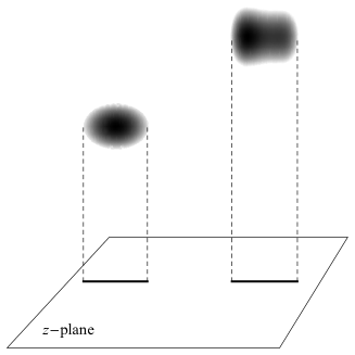
The lensing model corresponding to a $n$-cut eigenvalue distribution (22) can be applied to describe a system composed of $n$ edge-on disk galaxies [14]. These galaxies must be located on a common plane ($XY$-plane) orthogonal to the lens plane and such that their supports project to the intervals $[a_{i},b_{i}]$ in the lens plane with density $\rho(x)$ (Fig. 2). For example this is the case if the galaxies have uniform mass distributions supported on the domains $\mathcal{D}_{i}$ in the plane $XY$ bounded by the set of closed curves

$$Y^{2}=\frac{S_{i}^{2}}{4}\Big{(}\frac{m}{m_{i}}\Big{)}^{2}\,\rho(X)^{2},\quad a_{i}\leq X\leq b_{i},\quad i=1,\ldots,n,$$ (27)

where $S_{i}$ and $m_{i}$ are the area and the mass of $\mathcal{D}_{i}$, respectively.

Figure 2: The projected supports of coplanar edge-on galaxies is a union of intervals along a straight line on the lens plane.

3 The Gaussian model

The Gaussian matrix model is determined by the potential function

$$V(z)=\frac{z^{2}}{a^{2}},$$ (28)

where $a>0$ and constitutes a basic model in random matrix theory [11, 12, 13]. In this case there are only one-cut eigenvalue distributions, the function $P(z)$ in (11) is

$$P(z)=\frac{4}{a^{4}}(z^{2}-a^{2}),$$ (29)

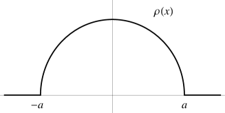
and the unit normalized mass density takes the form of the Wigner’s semi-circle law (Fig. 3)

$$\rho(x)=\frac{2}{\pi a^{2}}\sqrt{a^{2}-x^{2}},\quad-a\leq x\leq a.$$ (30)

Thus, the lens equation for a Gaussian lensing model of mass $m$ is

$$\left\{\begin{array}[]{ll}w=(1-p)x,\quad-a\leq x\leq a,\\ \\ \overline{w}=\overline{z}-p(z-\sqrt{z^{2}-a^{2}}),\quad z\in\mathbb{C}\setminus[-a,a],\end{array}\right.$$ (31)

where

$$p=\frac{2m}{a^{2}}.$$ (32)

Figure 3: Semicircle law of the Gaussian eigenvalue distribution.

3.1 The Gaussian model as a mother body for elliptic lenses

The mass distribution of the Gaussian lensing model of mass $m$

$$d\mu_{G}(x)=\frac{2m}{\pi a^{2}}\sqrt{a^{2}-x^{2}}\,dx,\quad-a\leq x\leq a,$$ (33)

is a mother body for $(D,\mu_{D})$ [19, 20] (see also Appendix A of this paper) where $\mu_{D}$ is the uniform mass distribution $d\mu_{D}=dx\,dy$ supported on the elliptic domain

$$D=\{(x,y)\in\mathbb{R}^{2},\,\frac{x^{2}}{\alpha^{2}}+\frac{y^{2}}{\beta^{2}}<1,\,\alpha>\beta,\beta>0\},$$ (34)

with focal distance $a=\sqrt{\alpha^{2}-\beta^{2}}$ and total mass $m=\pi\alpha\beta$.

3.2 The Gaussian model as an edge-on elliptic lens

According to the discussion of Subsection 2.5, the measure $\mu_{G}$ of the Gaussian model (33) describes an edge-on disk galaxy with uniform mass distribution of total mass $m$. The corresponding domain $\mathcal{D}$ in the $XY$-plane orthogonal to the lens plane is bounded by the closed curve with equation

$$Y^{2}=\frac{S^{2}}{\pi^{2}a^{4}}\,(a^{2}-X^{2}),\quad-a\leq X\leq a,$$ (35)

where $S$ is the area of $\mathcal{D}$. Thus $\mathcal{D}$ is an elliptic domain

$$\mathcal{D}=\{(X,Y)\in\mathbb{R}^{2},\,\frac{X^{2}}{a^{2}}+\frac{Y^{2}}{b^{2}}<1\},$$ (36)

with $b=S/\pi a$.

It is illustrative to provide an alternative direct proof of this interpretation of the Gaussian model starting from a well-known lensing model [21]. To this end we consider a uniform mass distribution of total mass $m$ on an elliptic domain in the lens $xy$-plane

$$D=\{(x,y)\in\mathbb{R}^{2},\,\frac{x^{2}}{a^{2}}+\frac{b^{2}}{b^{2}}<1,\,a>b,b>0\}.$$ (37)

The corresponding lens equation is [21]

$$\overline{w}=\overline{z}-\lambda\,\omega(z),\quad\lambda=\frac{m}{\pi a\,b},$$ (38)

where $\omega(z)$ is given by the expression (118) in Appendix A with $(\alpha,\beta)=(a,b)$, so that

$$\left\{\begin{array}[]{ll}\displaystyle\overline{w}=\overline{z}-\pi\lambda\Big{(}\overline{z}-\frac{(a-b)^{2}}{c^{2}}z\Big{)},\quad z\in D,\\ \\ \displaystyle\overline{w}=\overline{z}-\frac{2m}{c^{2}}\Big{(}z-\sqrt{z^{2}-c^{2}}\Big{)},\quad z\in\mathbb{C}\setminus\overline{D},\end{array}\right.$$ (39)

with $c^{2}=a^{2}-b^{2}$. If we perform a rotation of the ellipse plane of angle $\theta$ about the $x$-axis, the projected mass distribution on the lens plane is now supported on the elliptic domain

$$D^{\prime}=\{(x,y)\in\mathbb{R}^{2},\,\frac{x^{2}}{a^{2}}+\frac{y^{2}}{b^{\prime 2}}<1,\,b^{\prime}=b\cos\theta\},$$ (40)

and the lens equation reads

$$\left\{\begin{array}[]{ll}\displaystyle\overline{w}=\overline{z}-\pi\lambda^{\prime}\Big{(}\overline{z}-\frac{(a-b^{\prime})^{2}}{c^{\prime 2}}z\Big{)},\quad z\in D^{\prime},\\ \\ \displaystyle\overline{w}=\overline{z}-\frac{2m}{c^{\prime 2}}\Big{(}z-\sqrt{z^{2}-c^{\prime 2}}\Big{)},\quad z\in\mathbb{C}\setminus\overline{D^{\prime}},\end{array}\right.$$ (41)

where

$$c^{\prime 2}=a^{2}-b^{\prime 2},\quad\lambda^{\prime}=\frac{m}{\pi a\,b^{\prime}}.$$ (42)

If the inclination angle $\theta$ tends to $\pi/2$, then we are led to an edge-on galaxy with

$$a={\rm Constant},\quad b^{\prime}\rightarrow 0.$$ (43)

Thus $D^{\prime}$ shrinks to the interval $[-a,a]$ and

$$c^{\prime}\rightarrow a,\quad\pi\lambda^{\prime}\Big{(}1-\frac{(a-b^{\prime})^{2}}{c^{\prime 2}}\Big{)}\rightarrow\frac{2m}{a^{2}}.$$ (44)

Therefore, the lens equation (41) becomes exactly the lens equation (31) provided by the Gaussian model of mass $m$.

3.3 Solutions of the lens equation

From the first equation of (31) we have that there is a unique dim image $x=w/(1-p)$ for any source $w$ in the interval

$$-a\Big{|}1-p\Big{|}\leq w\leq a\Big{|}1-p\Big{|},$$ (45)

and no dim image otherwise. It should be noticed that for $p=1$ the whole interval $[-a,a]$ becomes the image of the origin $w=0$.

Let us now consider the lens equation (31) for bright images. The presence of the term with a square root suggests the introduction of a Joukowski change of variable

$$z=\frac{a}{2}\Big{(}Z+\frac{1}{Z}\Big{)},$$ (46)

which defines a conformal one-to-one map of the domain $\mathbb{C}\setminus[-a,a]$ in the $z$-plane onto the domain $|Z|<1$ in the $Z$-plane

$$Z=\frac{a}{z+\sqrt{z^{2}-a^{2}}}.$$ (47)

Thus the lens equation (31) for bright images becomes

$$Z^{2}-2p|Z|^{2}-2uZ+1=0,\quad|Z|<1,$$ (48)

where

$$u:=\frac{w}{a},$$ (49)

denotes the normalized source position. Then if we set

$$Z=\mathrm{x}+i\mathrm{y},\quad u=\alpha+i\beta,$$ (50)

we have that the solutions of (48) are the intersection points of the pair of conics

$$\left\{\begin{array}[]{ll}\beta\mathrm{x}+\alpha\mathrm{y}-\mathrm{x}\mathrm{y}=0,\\ \\ (1-2p)\,\mathrm{x}^{2}-(1+2p)\,\mathrm{y}^{2}-2(\alpha\mathrm{x}-\beta\mathrm{y})+1=0,\end{array}\right.$$ (51)

which satisfy

$$\mathrm{x}^{2}+\mathrm{y}^{2}<1.$$ (52)

Hence, we deduce that there are at most four bright images. Since $\mu_{G}$ is a mother body for a uniform distribution of an elliptic domain, this result is in agreement with Theorem 5.1 of [21]. We also note that the system (51) is invariant under the transformations $(\alpha,\mathrm{x})\leftrightarrow(-\alpha,-\mathrm{x})$ and $(\beta,\mathrm{y})\leftrightarrow(-\beta,-\mathrm{y})$ so that we may restrict our analysis to the first quadrant $\alpha\geq 0,\beta\geq 0$ of the $u$-plane.

If we eliminate $\mathrm{y}$ as $\mathrm{y}=\beta\mathrm{x}/(\mathrm{x}-\alpha)$ from the first equation of (51) and substitute the result into the second equation of (51), we get the following quartic equation for $\mathrm{x}$

$$(1-2p)\mathrm{x}^{4}+4\alpha(p-1)\mathrm{x}^{3}+(5\alpha^{2}+\beta^{2}-2p(\alpha^{2}+\beta^{2})+1)\mathrm{x}^{2}$$

$$-2\alpha(\alpha^{2}+\beta^{2}+1)\mathrm{x}+\alpha^{2}=0.$$ (53)

Then the solutions of (51) can be written as algebraic expressions in terms of the coefficients of (3.3).

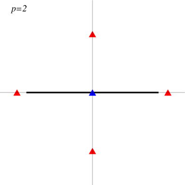
For example if $u=0$ and $p>1$ there are four distinct solutions of (51)-(52) (see Fig. 4): two purely imaginary

$$Z^{(1)}_{\pm}=\pm\frac{i}{\sqrt{1+2p}},$$ (54)

which determine two purely imaginary images in the $z$-plane

$$z^{(1)}_{\pm}=\mp i\frac{ap}{\sqrt{1+2p}},$$ (55)

and two real solutions

$$Z^{(2)}_{\pm}=\pm\frac{1}{\sqrt{2p-1}},$$ (56)

which determine two real images in the $z$-plane

$$z^{(2)}_{\pm}=\pm\frac{ap}{\sqrt{2p-1}}.$$ (57)

Figure 4: The Gaussian model for $p=2$ exhibits an Einstein cross of images of the source $w=0$, with four bright images (red triangles) and one dim images (blue triangle).

3.4 The case $p=1/2$

For $p=1/2$ the equation (3.3) reduces to a cubic equation and it is easy to complete the explicit analysis of the images.

The bright images for on-axis sources are as follows:

1. For $\alpha=\beta=0$ there are two solutions of (51) which satisfy (52) given by $Z_{\pm}=\pm i/\sqrt{2}$. They correspond to $z_{\pm}=\mp ia/(2\sqrt{2})$ in the $z$-plane.

2. For $\beta=0,\,\alpha\,>0$ there are three solutions of (51)

   $$Z_{\pm}=\alpha\pm i\sqrt{\frac{1}{2}-\alpha^{2}},\qquad Z_{0}=\frac{1}{2\alpha}.$$ (58)

   They satisfy (52) for the following values of $\alpha$

   $$\left\{\begin{array}[]{ll}Z_{\pm}&\mbox{if }\quad 0<\alpha\leq\frac{1}{2},\\ Z_{\pm},\,Z_{0}&\mbox{if }\quad\frac{1}{2}<\alpha<\frac{1}{\sqrt{2}},\\ Z_{0}&\mbox{if }\quad\alpha\geq\frac{1}{\sqrt{2}}.\end{array}\right.$$ (59)

   The corresponding solutions in the $z$-plane are

   $$z_{\pm}=\frac{a}{2}\Big{(}3\alpha\mp i\sqrt{\frac{1}{2}-\alpha^{2}}\Big{)},\qquad z_{0}=a\Big{(}\alpha+\frac{1}{4\alpha}\Big{)}.$$ (60)

3. For $\alpha=0\,,\beta\,>0$ the system (51) has two solutions

   $$\widehat{Z}_{\pm}=\frac{i}{2}\left(\beta\pm\sqrt{\beta^{2}+2}\right),$$ (61)

   which satisfy (52) for the following values of $\beta$

   $$\left\{\begin{array}[]{ll}\widehat{Z}_{\pm}&\mbox{if }\quad 0<\beta<\frac{1}{2},\\ \widehat{Z}_{-}&\mbox{if }\quad\beta\geq\frac{1}{2}.\end{array}\right.$$ (62)

   The corresponding solutions in the $z$-plane are

   $$\widehat{z}_{\pm}=i\,\frac{a}{4}\left(3\beta\mp\sqrt{\beta^{2}+2}\right).$$ (63)

The images for off-axis sources with

$$\alpha,\,\beta\,>0,$$ (64)

can be determined as follows. Since $\alpha$ and $\beta$ are different from zero, we have that $\mathrm{x}\neq\alpha$ and $\mathrm{y}=\beta\mathrm{x}/(\mathrm{x}-\alpha)$. Hence (3.3) reduces to the cubic equation

$$-2\alpha\mathrm{x}^{3}+(4\alpha^{2}+1)\mathrm{x}^{2}-2\alpha(\alpha^{2}+\beta^{2}+1)\mathrm{x}+\alpha^{2}=0.$$ (65)

The discriminant of the polynomial in this equation vanishes on the curve

$$16\alpha^{6}+8\alpha^{4}(4\beta^{2}-3)+4\alpha^{2}(4\beta^{4}+10\beta^{2}+3)-(\beta^{2}+2)=0.$$ (66)

Then, it is straightforward to deduce that

1. For $u$ outside the curve (66) there are one or three different solutions of (65).

2. For $u$ on the curve (66) there are two different solutions of (65).

Finally we have to determine which solutions of (65) satisfy the condition (52). Now from (51) it follows that $M=\mathrm{x}^{2}+\mathrm{y}^{2}$ satisfies the equation

$$16\alpha^{2}M^{3}-4(1+4\alpha^{2})M^{2}+4(1+\alpha^{2}+\beta^{2})M-1=0.$$ (67)

Then from Bolzano’s theorem it is immediate to deduce that one of the solutions of (67) satisfies $M<\frac{1}{2}$ . Moreover, for $|u|<1/2$ we have that at least one solution of (67) satisfies $\frac{1}{2}<M<1$, and for $|u|=1/2$ there exists a solution with $M=1$.

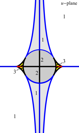
Therefore, we conclude that the number of bright images depends on the relative position $u$ of the source as shown in Fig. 5.

Figure 5: Number of bright images for the different positions of the source in the $u$-plane for the case $p=\frac{1}{2}$. Red, black and blue colors on the axes and on the curve stand for three, two and one bright images respectively. The different configurations are determined by the relative position of the source with respect to the curve (66) and the disk $|u|<1/2$.

3.5 Time delays

Using the expression (30) of the mass density we obtain the explicit form of the logarithmic potential

$$-\int_{-a}^{a}\rho(x)\ln|z-x|\,dx=-\frac{1}{a^{2}}\,{\rm Re}(z^{2}-z\sqrt{z^{2}-a^{2}})-\ln|z+\sqrt{z^{2}-a^{2}}|+\frac{1}{2}+\ln 2.$$ (68)

Hence, from (24) we may determine the time delay for bright images. In particular, for the bright images (55) and (57) of $w=0$ we have

$$\tau(z^{(1)}_{\pm})=\frac{m}{2}\Big{(}1+\ln\frac{1}{m+(a/2)^{2}}\Big{)},$$ (69)

$$\tau(z^{(2)}_{\pm})=\frac{m}{2}\Big{(}1+\ln\frac{1}{m-(a/2)^{2}}\Big{)},$$ (70)

so that the relative time delay for the reception of both pairs of images is given by

$$\tau(z^{(1)}_{\pm})-\tau(z^{(2)}_{\pm})=\frac{m}{2}\,\ln\Big{(}\frac{m-(a/2)^{2}}{m+(a/2)^{2}}\Big{)}.$$ (71)

4 The quartic model

We consider the quartic matrix model defined by the potential function

$$V(z)=\frac{z^{4}}{4}+t\,\frac{z^{2}}{2},$$ (72)

where $t$ is a real parameter. The corresponding eigenvalue distribution has a one-cut support for $t>-\sqrt{2}$ and a two-cut support for $t<-\sqrt{2}$ [13] (see also [22]). The value $t=-\sqrt{2}$ represents a point of phase transition.

4.1 The one-cut distribution

For $t>-\sqrt{2}$ the function $P(z)$ in (11) is given by

$$P(z)=(z^{2}-a^{2})(z^{2}+c)^{2},$$ (73)

where

$$a=\sqrt{\frac{2}{3}}\sqrt{-t+\sqrt{t^{2}+6}},\quad c=\frac{1}{3}\Big{(}2t+\sqrt{t^{2}+6}\Big{)}.$$ (74)

The associated mass density is (Fig. 6)

$$\rho(x)=\frac{1}{\pi}(x^{2}+c)\sqrt{a^{2}-x^{2}},\quad-a\leq x\leq a.$$ (75)

Figure 6: Eigenvalue density of the quartic model for several values of $t$ in the one-cut case.

4.2 The one-cut distribution as a mother body for elliptic lenses

As it is shown in the appendix A of this paper, the measure $d\mu_{Q}(x)=m\rho(x)dx$ determined by the density (75) is a mother body for the planar body $(D,\mu_{D})$ where $D$ is any elliptic domain $D$ (34) contained in the region

$$y^{2}<x^{2}+\frac{c_{3}}{2c_{2}},$$ (76)

with

$$c_{2}=\frac{3}{3A_{1}^{2}+A_{2}^{2}+3},\quad c_{3}=c+\frac{a^{2}A_{2}^{2}}{3A_{1}^{2}+A_{2}^{2}+3},$$ (77)

$$A_{1}=\frac{\alpha^{2}+\beta^{2}}{a^{2}},\quad A_{2}=-2\frac{\alpha\beta}{a^{2}},\quad a^{2}=\alpha^{2}-\beta^{2},$$ (78)

and $\mu_{D}$ is the measure supported on $D$ given by

$$d\mu_{D}(x,y)=\frac{m}{\pi|A_{2}|}\Big{(}2c_{2}(x^{2}-y^{2})+c_{3}\Big{)}dxdy.$$ (79)

4.3 The one-cut distribution as an edge-on lens

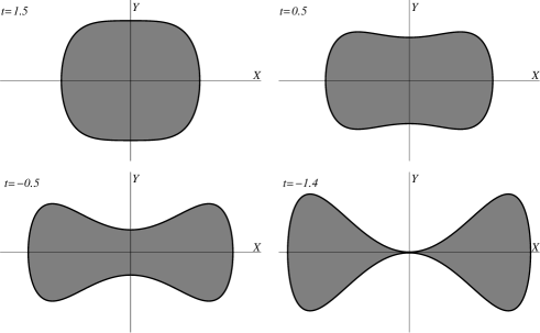
According to (27) the one-cut distribution $d\mu_{Q}(x)=m\rho(x)dx$ of the quartic model describes an edge-on lens with a uniform mass distribution of total mass $m$ on the region $\mathcal{D}$ of the $XY$-plane bounded by the curve

$$Y^{2}=\frac{S^{2}}{4\pi^{2}}(X^{2}+c)^{2}(a^{2}-X^{2}),\quad-a<X<a,$$ (80)

where $S$ is the area of $\mathcal{D}$ (Fig. 7).

Figure 7: Edge-on galaxies for the quartic model in the one-cut case.

4.4 Solutions of the lens equation in the one-cut case

The lens equation in the one-cut case takes the form

$$\left\{\begin{array}[]{ll}w=x-m(x^{3}+tx),\quad-a\leq x\leq a,\\ \\ \overline{w}=\overline{z}-m\Big{(}z^{3}+tz-(z^{2}+c)\sqrt{z^{2}-a^{2}}\Big{)},\quad z\in\mathbb{C}\setminus[-a,a].\end{array}\right.$$ (81)

We will concentrate on the images produced by the source $w=0$.

The dim images for $w=0$ are the solutions of

$$x\left[mx^{2}+(mt-1)\right]=0,\quad x\in[-a,a].$$ (82)

This equation has always the solution $x^{(0)}=0$. Furthermore, if one of the two pairs of conditions

$$\begin{array}[]{l}m>\frac{1}{\sqrt{2}},\quad t\in[-\sqrt{2},\frac{1}{m}),\\ m\in(0,\frac{1}{\sqrt{2}}],\quad t\in[t_{c},\frac{1}{m}),\end{array}$$ (83)

is satisfied, where

$$t_{c}=\frac{2\sqrt{1-2m^{2}}-1}{m},$$ (84)

then there is a pair of additional images

$$x^{(d)}_{\pm}=\pm\sqrt{\frac{1}{m}-t}.$$ (85)

The bright images of $w=0$ are characterized by the equation

$$m(z^{3}+tz)-\overline{z}=m(z^{2}+c)\sqrt{z-a}\sqrt{z+a},\quad z\in{\mathbb{C}}\setminus[-a,a],$$ (86)

where we assume the principal branch for both square roots. It is easy to check that (86) has not off-axis solutions. The bright images $x$ on the real axis satisfy

$$\left\{\begin{array}[]{ll}mx^{3}+(mt-1)x=m(x^{2}+c)\sqrt{x^{2}-a^{2}},&\mbox{if }\;x>a,\\ mx^{3}+(mt-1)x=-m(x^{2}+c)\sqrt{x^{2}-a^{2}},&\mbox{if }\;x<-a.\end{array}\right.$$ (87)

Then there exist two solutions $x^{(1)}_{\pm}$ $(x^{(1)}_{-}=-x^{(1)}_{+})$ if and only if one of the following three pairs of conditions is verified :

$$\begin{array}[]{l}m>\frac{1}{\sqrt{2}},\quad t\in[-\sqrt{2},\infty),\\ m=\frac{1}{\sqrt{2}},\quad t\in(-\sqrt{2},\infty),\\ m\in(0,\frac{1}{\sqrt{2}}),\quad t\in(t_{c},\infty).\end{array}$$ (88)

Note that $t_{c}>-\sqrt{2}$ if $m<\frac{1}{\sqrt{2}}$.

The bright images $i\,y\,(y\neq 0)$ on the imaginary axis are the solutions of

$$\left\{\begin{array}[]{ll}-my^{3}+(mt+1)y=m(c-y^{2})\sqrt{y^{2}+a^{2}},&\mbox{if }\,y>0,\\ -my^{3}+(mt+1)y=-m(c-y^{2})\sqrt{y^{2}+a^{2}},&\mbox{if }\,y<0.\end{array}\right.$$ (89)

Then, it follows that there are two solutions $iy^{(1)}_{\pm}$ $(y^{(1)}_{-}=-y^{(1)}_{+})$ if and only if one of the following two pairs of conditions is verified:

$$\begin{array}[]{l}m>\frac{1}{\sqrt{2}},\quad t\in[-\sqrt{2},\infty),\\ m\in(0,\frac{1}{\sqrt{2}}],\quad t\in(-\sqrt{2},\infty).\end{array}$$ (90)

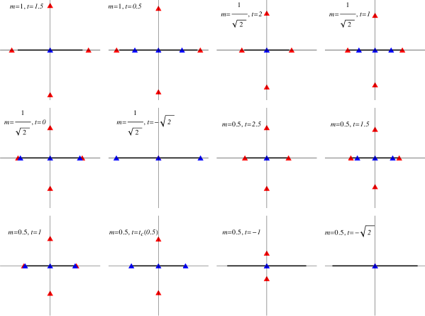
Figure 8: Sets of images of $w=0$ in the one cut case. The first two figures of the first row correspond to $m=1>1/\sqrt{2}$ and represent an Einstein cross at $t=1.5>1/m$ which becomes accompanied by a couple of dim images at $t=0.5<1/m$. The next four figures illustrate the case $m=1/\sqrt{2}$. They show an Einstein cross at $t=2>\sqrt{2}$ and a couple of dim images which arises for $t<\sqrt{2}$ and move, together with the two bright images on the real axis, to the endpoints of the lens at $t=-\sqrt{2}$. All the bright images dissapear at $t=-\sqrt{2}$. Finally, the last six figures for $m=0.5<1/\sqrt{2}$ show a process in which two dim images and two bright images move towards the endpoints of the lens. For $t<t_{c}$ only the dim image at the origin and the two bright images on the imaginary axis appear. These last two images vanish at $t=-\sqrt{2}$.

In conclusion, the images of $w=0$ in the one-cut case are classified into the following cases (Fig. 8):

$$\begin{array}[]{lll}m>\frac{1}{\sqrt{2}}\,:&x^{(0)},\,x^{(1)}_{\pm},\;iy^{(1)}_{\pm}&\mbox{for}\quad t\geq\frac{1}{m},\\ &x^{(0)},\,x^{(d)}_{\pm},\,x^{(1)}_{\pm},\;iy^{(1)}_{\pm}&\mbox{for}\quad t\in\left[-\sqrt{2},\frac{1}{m}\right),\\ \\ m=\frac{1}{\sqrt{2}}\,:&x^{(0)},\,x^{(1)}_{\pm},\,iy^{(1)}_{\pm}&\mbox{for}\quad t\geq\sqrt{2},\\ &x^{(0)},\;x^{(d)}_{\pm},\,x^{(1)}_{\pm},\;iy^{(1)}_{\pm}&\mbox{for}\quad t\in(-\sqrt{2},\sqrt{2}),\\ &x^{(0)},\;x^{(d)}_{\pm}&\mbox{for}\quad t=-\sqrt{2},\\ \\ m\in\left(0,\frac{1}{\sqrt{2}}\right)\,:&x^{(0)},\,x^{(1)}_{\pm},\;iy^{(1)}_{\pm}&\mbox{for}\quad t\geq\frac{1}{m},\\ &x^{(0)},\;x^{(d)}_{\pm},\,x^{(1)}_{\pm},\;iy^{(1)}_{\pm}&\mbox{for}\quad t\in\left(t_{c},\frac{1}{m}\right),\\ &x^{(0)},\;x^{(d)}_{\pm},\,iy^{(1)}_{\pm}&\mbox{for}\quad t=t_{c},\\ &x^{(0)},\,iy^{(1)}_{\pm}&\mbox{for}\quad t\in(-\sqrt{2},t_{c}),\\ &x^{(0)}&\mbox{for}\quad t=-\sqrt{2}.\end{array}$$ (91)

4.5 The two-cut distribution

For $t<-\sqrt{2}$ the quartic matrix model exhibits a two-cut distribution ([13], [22]) such that the function $P(z)$ in (11) is

$$P(z)=z^{2}(z^{2}-a^{2})(z^{2}-b^{2}),$$ (92)

where

$$a=\sqrt{\sqrt{2}-t},\quad b=\sqrt{-\sqrt{2}-t}.$$ (93)

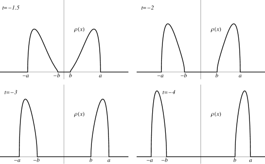
It leads to a mass density (Fig. 9):

$$\rho(x)=\frac{|x|}{\pi}\sqrt{(a^{2}-x^{2})(x^{2}-b^{2})},\quad x\in[-a,-b]\cup[b,a],$$ (94)

and to a Cauchy transform

$$\omega(z)=z^{3}+tz-z\sqrt{(z^{2}-a^{2})(z^{2}-b^{2})}.$$ (95)

Figure 9: Eigenvalue densities of the quartic model in the two-cut case.

4.6 The two-cut distribution as an edge-on double lens

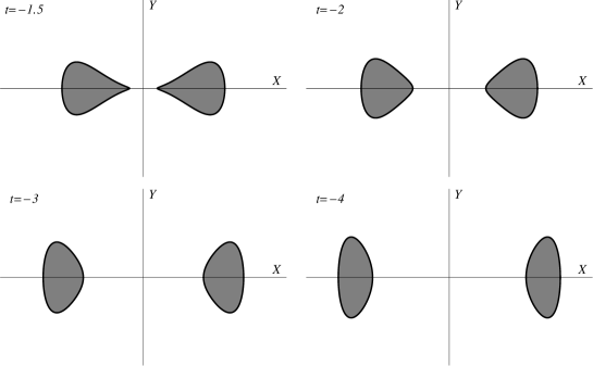
According to (27) the two cut distribution of the quartic model describes an edge-on lens composed by two twin galaxies with a uniform mass distribution of total mass $m$ supported on the regions $\mathcal{D}_{\pm}$ of the $XY$-plane bounded by the two-component curve

$$Y^{2}=\frac{S^{2}}{4\pi^{2}}X^{2}(a^{2}-X^{2})(X^{2}-b^{2}),\quad x\in[-a,-b]\cup[b,a],$$ (96)

where $S$ is the area of $\mathcal{D}_{-}\cup\mathcal{D}_{+}$ (Fig. 10).

Figure 10: Edge on galaxies for the quartic model in the two cut case.

4.7 Solutions of the lens equation in the two-cut case

The lens equation for the two-cut distribution is

$$\left\{\begin{array}[]{ll}w=x-m(x^{3}+tx),\quad x\in[-a,-b]\cup[b,a],\\ \\ \overline{w}=\overline{z}-m\Big{(}z^{3}+tz-z\sqrt{(z^{2}-a^{2})(z^{2}-b^{2})}\Big{)},\quad z\in\mathbb{C}\setminus\Big{(}[-a,-b]\cup[b,a]\Big{)}.\end{array}\right.$$ (97)

We again concentrate on the images of the source $w=0$.

The dim images are the solutions of the equation

$$m(x^{2}+t)-1=0,\quad x\in[-a,-b]\cup[b,a].$$ (98)

Then if $m\geq\frac{1}{\sqrt{2}}$ we have two dim images at the positions

$$x_{\pm}^{(d)}=\pm\sqrt{\frac{1}{m}-t},$$

and no dim images otherwise.

The bright images of $w=0$ satisfy

$$\overline{z}-m\Big{(}z^{3}+tz-z\sqrt{(z^{2}-a^{2})(z^{2}-b^{2})}\Big{)}=0,\quad z\in{\mathbb{C}}\setminus\Big{(}[-a,-b]\cup[b,a]\Big{)}.$$ (99)

Again, a direct computation shows that (99) has not off-axis solutions.

The real solution $x^{(0)}=0$ is now a bright image and from (93) it can be easily seen that other real solutions $x$ must satisfy

$$\left\{\begin{array}[]{ll}mx^{2}+(mt-1)=m\sqrt{(x^{2}+t)^{2}-2},&\mbox{if }\;|x|>a,\\ mx^{2}+(mt-1)=-m\sqrt{(x^{2}+t)^{2}-2},&\mbox{if }\;|x|<b.\end{array}\right.$$ (100)

It turns out that there are not solutions such that $|x|<b$. Nevertheless, for $m>\frac{1}{\sqrt{2}}$ the solutions $|x|>a$ are given by

$$x_{\pm}^{(2)}=\pm\sqrt{m+\frac{1}{2m}-t}.$$

The bright images $z=iy$, $(y\neq 0)$ on the imaginary axis satisfy

$$my^{2}-(mt+1)=m\sqrt{(y^{2}-t)^{2}-2}.$$ (101)

Then we get the solutions

$$iy_{\pm}^{(2)}=\pm i\sqrt{m+\frac{1}{2m}+t},$$ (102)

provided $m>1/\sqrt{2}$ and $t\in\left(-m-\frac{1}{2m},-\sqrt{2}\right).$

Summarizing, the dim and bright images of $w=0$ in the two-cut case are

$$\begin{array}[]{lll}m>\frac{1}{\sqrt{2}}\,:&x^{(0)},\,x^{(d)}_{\pm},\,x^{(2)}_{\pm},\,iy^{(2)}_{\pm}&\mbox{for}\quad t\in\left(-m-\frac{1}{2m},-\sqrt{2}\right),\\ &x^{(0)},\,x^{(d)}_{\pm},\,x^{(2)}_{\pm},&\mbox{for}\quad t\leq-m-\frac{1}{2m},\\ \\ m=\frac{1}{\sqrt{2}}\,:&x^{(0)},\;x^{(d)}_{\pm}=\pm a,&\\ \\ m<\frac{1}{\sqrt{2}}\,:&x^{(0)}.&\end{array}$$ (103)

4.8 A calculation of a relative time delay

As an example to show how to calculate relative time delays of explicit solutions of the lens equation we consider

$$\tau(iy_{\pm}^{(2)})-\tau(0)=\frac{(y_{\pm}^{(2)})^{2}}{2}+m\,\Big{(}U(iy_{\pm}^{(2)})-U(0)\Big{)},$$ (104)

where $iy_{\pm}^{(2)}$ (102) and $x^{(0)}=0$ are the bright images of $w=0$ in the two-cut case for $m>\frac{1}{\sqrt{2}}$ and $t\in(-m-\frac{1}{2m},-\sqrt{2})$. We observe that taking into account that

$$\partial_{y}U(iy)=-\int_{\Gamma}\rho(s)\frac{y}{y^{2}+s^{2}}ds,$$ (105)

we have

$$U(iy)-U(0)=-\frac{i}{2}\int_{0}^{y}\Big{(}\omega(is)-\omega(-is)\Big{)}\,ds.$$ (106)

Then, from (95) and (106) we obtain

$$\tau(iy_{\pm}^{(2)})-\tau(0)=\frac{(y_{\pm}^{(2)})^{2}}{2}-m\,\int_{0}^{y_{\pm}^{(2)}}\Big{(}s^{3}-ts-s\sqrt{(s^{2}-t)^{2}-2}\Big{)}\,ds$$

$$=\frac{1}{8m}\Big{[}1+4mt-4m^{2}\ln m+2m^{2}\left(1+t^{2}+t\sqrt{t^{2}-2}\right)$$ (107)

$$\quad-4m^{2}\ln\left(-t-\sqrt{t^{2}-2}\right)\Big{]}.$$ (108)

4.9 The phase transition

It is worth analyzing the behaviour of the images of $w=0$ at the phase transition $t=-\sqrt{2}$ for the different values of the total mass $m$.

For $m>\frac{1}{\sqrt{2}}$ it is easily found that

$$\lim_{t\rightarrow-\sqrt{2}^{+}}x^{(1)}_{\pm}=\lim_{t\rightarrow-\sqrt{2}^{-}}x^{(2)}_{\pm},\quad\lim_{t\rightarrow-\sqrt{2}^{+}}y^{(1)}_{\pm}=\lim_{t\rightarrow-\sqrt{2}^{-}}y^{(2)}_{\pm}.$$ (109)

Thus the only effect on the set of images at the phase transition is the change from dim to bright image of $x^{(0)}=0$.

For $m=\frac{1}{\sqrt{2}}$ the image positions satisfy

$$\lim_{t\rightarrow-\sqrt{2}^{+}}x^{(1)}_{\pm}=\lim_{t\rightarrow-\sqrt{2}^{+}}x^{(d)}_{\pm}=\pm a,\quad\lim_{t\rightarrow-\sqrt{2}^{+}}y^{(1)}_{\pm}=0,$$

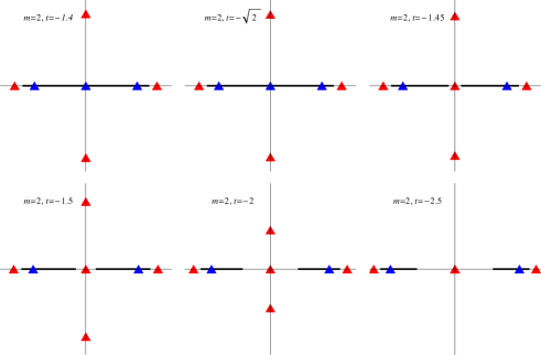
so that the four bright images $x^{(1)}_{\pm}$, $iy^{(1)}_{\pm}$ which arise in the one-cut case disappear at $t=-\sqrt{2}$. Furthermore, the dim images $x^{(d)}_{\pm}$ of the one-cut case stay at $\pm a$ for $t<-\sqrt{2}$. As in the previous case, the dim image at $x^{(0)}=0$ in the one-cut case becomes bright in the two-cut phase.

Finally, for $m\in(0,\frac{1}{\sqrt{2}})$ we have that according to (91) the images of $w=0$ for $t\in(-\sqrt{2},t_{c})$ are $x^{(0)}=0$ (dim) and $iy^{(1)}_{\pm}$ (bright). Again

$$\lim_{t\rightarrow-\sqrt{2}^{+}}iy^{(1)}_{\pm}=0,$$

and these images disappear in the two-cut phase. Also as in the previous cases the dim image at $x^{(0)}=0$ becomes bright. These features of the phase transition are shown in Fig. 11.

Figure 11: Images for $w=0$ in the phase transition of the quartic model. The first figure corresponds to $t=-1.4$ just before the phase transition, we can observe an Einstein cross of images and a couple of dim images. Once the phase transition has occurred at $t=-\sqrt{2}$ (third to the sixth figures) the dim image at the origin has become bright. Moreover, the two bright images on the imaginary axis move towards the origin where they disappear at $t=-2.25$.

Concluding remarks

In this paper we have presented several results on the possible applications of the eigenvalue distributions of random matrix models to gravitational lensing. We finish our discussion by raising several open problems.

From (23) it is clear that for a lensing model corresponding to a unitary ensemble with potential $V(x)$ of degree $2p>2$ the number of dim images cannot exceed $2p-1$ and that this bound is sharp. On the other hand, from (23) and taking (11) into account, Bezout theorem leads to the upper bound $4p^{2}$ for the number of bright images. Although this bound is sharp for the Gaussian model it would be interesting to improve it for the general case.

The present paper focuses on lensing models based on eigenvalue distributions of unitary ensembles of random matrices. Nevertheless, lensing models with similar properties can be generated from more general ensembles of random matrices [23],[24],[25] in which the eigenvalues are constrained to lie on appropriate curves. It remains to know the interpretation of the associated lensing models.

As it is well known [26] the eigenvalue distributions of random matrices of large size are closely connected to asymptotic distributions of zeros of associated families of orthogonal polynomials. Thus it is possible to formulate the analysis of this paper using zero distributions of orthogonal polynomials instead of eigenvalue distributions of random Hermitian matrices. More generally, since the main properties of these mass distributions derive from the fact that they minimize the energy functional, we may generalize our analysis to continuous critical measures in the sense of Martínez-Finkelstein and Rakhmanov [27], which are saddle points for energy functionals.

Appendix A: Eigenvalue distributions as mother bodies on elliptic domains

We next analyze the two examples of mother bodies for measures supported on elliptic domains which appear in this work.

Let $D$ be the elliptic domain

$$D=\{(x,y)\in\mathbb{R}^{2},\,\frac{x^{2}}{\alpha^{2}}+\frac{y^{2}}{\beta^{2}}<1,\,\alpha>\beta,\beta>0\}.$$ (110)

In our next calculation we describe the ellipse $\delta D$ in terms of the equation

$$\overline{z}=S(z),$$ (111)

where $S(z)$ is the Schwarz function of the ellipse [20]

$$S(z)=\frac{\alpha^{2}+\beta^{2}}{a^{2}}z-i\frac{2\alpha\beta}{a^{2}}\sqrt{a^{2}-z^{2}},\quad(a^{2}:=\alpha^{2}-\beta^{2}).$$ (112)

We also use the generalized Cauchy formula

$$\int_{D}\frac{\overline{\partial}f(\zeta,\overline{\zeta})}{z-\zeta}\,d^{2}\zeta=\pi\,n(\delta D,z)\,f(z,\bar{z})+\frac{1}{2i}\int_{\delta D}\frac{f(\zeta,\overline{\zeta})}{z-\zeta}\,d\zeta,\quad z\in\mathbb{C}\setminus{\delta D},$$ (113)

for a smooth function $f(z,\bar{z})$ on $\overline{D}$, where $n(\delta D,z)$ is the index of $z$ with respect to $\delta D$, $\overline{\partial}=\partial/\partial\overline{z}$ and $d^{2}\zeta$ stands for the Lebesgue measure in the plane.

The Gaussian model

Let $\mu_{D}$ be the measure defined by a uniform mass density $d\mu_{D}=dx\,dy$ on $D$. Then from (111) and (113) it follows that its Cauchy transform satisfies

$$\omega(z)=\int_{D}\frac{d^{2}\zeta}{z-\zeta}=\frac{1}{2i}\int_{\delta D}\frac{S(\zeta)}{z-\zeta}d\zeta,\,\,z\in\mathbb{C}\setminus\overline{D}.$$ (114)

If we deform $\delta D$ into the interval $[-a,a]$ and use the expression (112) of $S(z)$ we obtain

$$\omega(z)=\frac{2\alpha\beta}{a^{2}}\int_{-a}^{a}\frac{\sqrt{a^{2}-x^{2}}}{z-x}\,dx,\quad z\in\mathbb{C}\setminus\overline{D}.$$ (115)

The last integral is the Cauchy transform of the measure

$$d\mu_{G}(x)=\frac{2\alpha\beta}{a^{2}}\sqrt{a^{2}-x^{2}}\,dx,\quad-a\leq x\leq a,$$ (116)

which coincides with the mass distribution of the Gaussian model of total mass $m=\pi\alpha\beta$. Consequently, $\mu_{G}$ is a mother body measure for $\mu_{D}$. In fact it can be proved [9] that it is the unique mother body for $\mu$.

From the generalized Cauchy formula, the Cauchy transform of $\mu_{D}$ on $\mathbb{C}\setminus\delta D$ can be calculated [21] in the form

$$\int_{D}\frac{d^{2}\zeta}{z-\zeta}=\left\{\begin{array}[]{ll}\displaystyle\pi\overline{z}+\frac{1}{2i}\int_{\delta D}\frac{\overline{\zeta}}{z-\zeta}d\zeta,\quad z\in D,\\ \\ \displaystyle\frac{1}{2i}\int_{\delta D}\frac{\overline{\zeta}}{z-\zeta}d\zeta,\quad z\in\mathbb{C}\setminus\overline{D},\end{array}\right.$$ (117)

so that taking (112) into account we obtain

$$\omega(z)=\left\{\begin{array}[]{ll}\displaystyle\pi\overline{z}-\pi\frac{(\alpha-\beta)^{2}}{a^{2}}z,\quad z\in D,\\ \\ \displaystyle\frac{2\pi\alpha\beta}{a^{2}}\Big{(}z-\sqrt{z^{2}-a^{2}}\Big{)},\quad z\in\mathbb{C}\setminus\overline{D}.\end{array}\right.$$ (118)

The quartic potential model

We now consider the mass distribution of the quartic potential model with mass $m$ in the one-cut case (75)

$$d\mu_{Q}(x)=\frac{m}{\pi}(x^{2}+c)\sqrt{a^{2}-x^{2}}\,dx,\quad-a\leq x\leq a,$$ (119)

where the parameters $a$ and $c$ are given by (74). Let $D$ be an elliptic domain (36) with $\alpha^{2}-\beta^{2}=a^{2}$, and let us look for a measure $d\mu=\rho(z,\overline{z})d^{2}z$ on $D$ defining the same Cauchy transform as $d\mu_{Q}$ outside $D$. Assume a density of the form $\rho=-i\overline{\partial}f$ where $f=f(z,\overline{z})$ is a polynomial such that its restriction to $\delta D$ is given by

$$f(z,\overline{z})=\frac{m}{\pi}(z^{2}+c)\sqrt{a^{2}-z^{2}}+g(z),\quad\forall z\in\delta D,$$ (120)

where $g(z)$ is some polynomial in $z$. Then, from (113) and deforming $\delta D$ into the interfocal interval $[-a,a]$ we have that the function $f$ must satisfy

$$-i\int_{D}\frac{\overline{\partial}f(\zeta,\overline{\zeta})}{z-\zeta}d^{2}\zeta=\int_{-a}^{a}\frac{d\mu_{Q}(x)}{z-x},\quad z\in\mathbb{C}\setminus\overline{D}.$$ (121)

Taking into account that the expression (112) of the Schwarz function for the ellipse can be written as $S(z)=A_{1}z+iA_{2}\sqrt{a^{2}-z^{2}}$ where

$$A_{1}=\frac{\alpha^{2}+\beta^{2}}{a^{2}},\quad A_{2}=-2\frac{\alpha\beta}{a^{2}},\quad a^{2}=\alpha^{2}-\beta^{2},$$ (122)

it is straightforward to see that a polynomial of the form

$$f(z,\overline{z})=\frac{m}{i\pi A_{2}}(c_{1}\overline{z}^{3}+c_{2}z^{2}\overline{z}+c_{3}\overline{z}),$$ (123)

verifies (120) if

$$(3A_{1}^{2}+A_{2}^{2})c_{1}+c_{2}=1,\quad c_{3}-a^{2}A_{2}^{2}c_{1}=c.$$ (124)

Moreover, (123) implies

$$-i\overline{\partial}f(z,\overline{z})=\frac{m}{\pi|A_{2}|}(3c_{1}\overline{z}^{2}+c_{2}z^{2}+c_{3}),$$ (125)

so that $-i\overline{\partial}f$ is a real-valued function if

$$c_{2}=3c_{1}.$$ (126)

Thus from (124) and (126) we deduce that a polynomial of the form (123) satisfies (120) and determines a real-valued expression for $-i\overline{\partial}f$ provided

$$c_{1}=\frac{1}{3A_{1}^{2}+A_{2}^{2}+3},\quad c_{2}=\frac{3}{3A_{1}^{2}+A_{2}^{2}+3},\quad c_{3}=c+\frac{a^{2}A_{2}^{2}}{3A_{1}^{2}+A_{2}^{2}+3}.$$ (127)

In this case we have

$$-i\overline{\partial}f(\zeta,\overline{\zeta})=\frac{m}{\pi|A_{2}|}\Big{(}2c_{2}(x^{2}-y^{2})+c_{3}\Big{)},$$ (128)

so that for an elliptic region $D$ (36) inside the open set

$$y^{2}<x^{2}+\frac{c_{3}}{2c_{2}},$$ (129)

it follows that $-i\overline{\partial}f$ is positive on $D$. Then $d\mu_{D}=-i\overline{\partial}f(z,\overline{z})d^{2}z$ determines a measure supported on $D$. Moreover, from (121) we have that the Cauchy transforms of $\mu_{Q}$ and $\mu_{D}$ coincide on $\mathbb{C}\setminus\overline{D}$, and therefore it implies that $\mu_{Q}$ is a mother body measure for $\mu_{D}$.

It is easy to see that a sufficient condition for $D$ to be contained inside the region (129) is

$$\beta^{2}<\frac{a^{2}}{6}A_{2}^{2}=\frac{2}{3}\frac{\alpha^{2}\beta^{2}}{\alpha^{2}-\beta^{2}},$$ (130)

or, equivalently, $\alpha/\sqrt{3}<\beta<\alpha$.

References

• [1] Schneider P, Helers J and Falco E 1992 Gravitational Lenses (Springer Verlag)
• [2] Narayan R and Bartelmann M 1996 Lectures on gravitational lensing Proceedings of the 1995 Jerusalem Winter School ed Dekel A and Ostriker J P (Cambridge University Press)
• [3] Einstein A 1936 Science 84
• [4] Straumann N 1997 Helvetica Physica Acta 70 894–908
• [5] Bleher P, Homma Y, Ji L and Roeder R K W 2014 Internat. Math. Res. Notices 8 2245–2264
• [6] Schneider P and Weiss A 1986 Astronomy and Astrophysics 164 237–259
• [7] Zidarov D 1968 On Solution of Some Inverse Problems for Potential Fields and its Application to Questions in Geophysics (Sofia: Publ. House of Bulg. Acad. of Sci. (Russian))
• [8] Gustafsson B 1998 SIAM Journal on Mathematical Analysis 29 1106
• [9] Sabina T V, Sternin B Y and Shatalov V E 2005 Appl. Anal. 84 649
• [10] Bogvad R and Shapiro B 2016 L’Enseignement Mathematique 62 117–142
• [11] Mehta M L 1991 Random Matrices (New York: Academic Press)
• [12] Di Francesco P, Ginsparg P and Zinn-Justin J 1995 Phys. Rep. 254 1–133
• [13] Bleher P 2008 Lectures on random matrix models. The Riemann-Hilbert approach (Amsterdam: North Holland)
• [14] Kautsch S, Grebel E K, Barazza F D and III J S G 2006 Astronomy and Astrophysics 445 765
• [15] Álvarez G, Martínez Alonso L and Medina E 2010 J. Stat. Mech. Theory Exp. 03023
• [16] Martínez-Finkelshtein A, Orive R and Rakhmanov E A 2015 Commun. Math. Phys. 333 1109–1173
• [17] Henrici P 1993 Applied and Computational Complex Analysis vol 3 (John wiley and sons)
• [18] Ablowitz M J and Fokas A S 2003 Complex variables: Introduction and applications second edition ed (Cambridge University Press)
• [19] Sjodin T 2006 Complex Variables and Elliptic Equations 51 357
• [20] Shapiro H S 1992 The Schwarz Function and its Generalization to Higher Dimensions (Univ. of Arkansas Lect. Notes Math. Vol. 9, Wiley N.Y.)
• [21] Fassnacht C, Keeton C and Khavinson D 2009 Gravitational lensing by elliptic galaxies, and the Schwarz function. Analysis and Mathematical Physics Trends in Mathematics. (Birkhuser, Basel)
• [22] Bleher P and Its A 2003 Commun. Pure Appl. Math. 56 433–516
• [23] Álvarez G, Martínez Alonso L and Medina E 2013 J. Stat. Mech. Theory Exp. 06 P06006
• [24] Álvarez G, Martínez Alonso L and Medina E 2015 Ann. Phys. 361 440–460
• [25] Álvarez G, Martínez Alonso L and Medina E 2017 J. Phys. A: Math. and Theor. 50 125203
• [26] Deift P 1999 Orthogonal Polynomials and Random Matrices: A Riemann–Hilbert approach (Providence: American Mathematical Society)
• [27] Martínez-Finkelshtein A and Rakhmanov E A 2011 Commun. Math. Phys. 302 53–111