Renormalization group analysis of dipolar Heisenberg model on square lattice

Abstract

We present a detailed functional renormalization group analysis of spin-1/2 dipolar Heisenberg model on square lattice. This model is similar to the well known $J_{1}$-$J_{2}$ model and describes the pseudospin degrees of freedom of polar molecules confined in deep optical lattice with long-range anisotropic dipole-dipole interactions. Previous study of this model based on tensor network ansatz indicates a paramagnetic ground state for certain dipole tilting angles which can be tuned in experiments to control the exchange couplings. The tensor ansatz formulated on a small cluster unit cell is inadequate to describe the spiral order, and therefore the phase diagram at high azimuthal tilting angles remains undetermined. Here we obtain the full phase diagram of the model from numerical pseudofermion functional renormalization group calculations. We show that an extended quantum paramagnetic phase is realized between the Néel and stripe/spiral phase. In this region, the spin susceptibility flows smoothly down to the lowest numerical renormalization group scales with no sign of divergence or breakdown of the flow, in sharp contrast to the flow towards the long-range ordered phases. Our results provide further evidence that the dipolar Heisenberg model is a fertile ground for quantum spin liquids.

I Introduction

A paradigmatic model for frustrated quantum magnetism is the $J_{1}$-$J_{2}$ model on square lattice. It is defined as a spin-1/2 Heisenberg model with antiferromagnetic nearest neighbor ($J_{1}$) and next-nearest neighbor ($J_{2}$) exchange couplings, described by the Hamiltonian

$$H_{J_{1}J_{2}}=J_{1}\sum_{\langle ij\rangle}\mathbf{S}_{i}\cdot\mathbf{S}_{j}+J_{2}\sum_{\langle\langle ij\rangle\rangle}\mathbf{S}_{i}\cdot\mathbf{S}_{j}.$$ (1)

Here the first (second) sum is over the nearest (next nearest) neighbors and $\mathbf{S}_{i}=(S_{i}^{x},S_{i}^{y},S_{i}^{z})$ are the usual spin-1/2 operators at site $i$. Although the limits of small and large $J_{2}/J_{1}$ are well understood to have long-range Néel and columnar orders respectively, the ground state near the maximally frustrated regime $J_{2}\sim 0.5J_{1}$ is still controversial (see Refs. Richter and Schulenburg, 2009; Jiang et al., 2012; Hu et al., 2013; Wang et al., 2013; Gong et al., 2014; Wang et al., 2016 and references therein). There is strong evidence that it is likely a quantum spin liquid which does not have any conventional magnetic long range order and does not break the symmetry of the Hamiltonian. Quantum spin liquids manifest a series of novel properties such as topological order and excitations with fractional statistics Savary and Balents (2016); Lee (2014); Zhou et al. (2017). They are of great interest to strongly correlated electron systems including copper oxide superconductors Anderson (1987) and frustrated quantum magnets Savary and Balents (2016); Lee (2014); Zhou et al. (2017). An ensuing theoretical challenge is to identify realistic physical models that can be realized cleanly in experiments and find the parameter regions in the phase diagram where a spin liquid arises.

Recent work examined the phase diagram of dipolar Heisenberg model on square lattice and found evidence for a possible spin liquid phase Zou et al. (2017). The dipolar Heisenberg model can be viewed as a close cousin of $H_{J_{1}J_{2}}$ but with a larger parameter space and important distinctions. Its Hamiltonian is given by

$$H_{\hat{d}}=\sum_{i_{1}\neq i_{2}}J_{\hat{d}}(i_{1},i_{2})\mathbf{S}_{i_{1}}\cdot\mathbf{S}_{i_{2}},$$ (2)

where the summation is over all pairs of sites, labelled by the site index $i_{1}$ and $i_{2}$, within the two-dimensional square lattice on the $xy$ plane (Fig. 1). This all-to-all coupling differs from the $J_{1}$-$J_{2}$ model. The spin exchange has the following dipolar interaction form

$$J_{\hat{d}}(i_{1},i_{2})=J_{0}[1-3(\hat{r}_{i_{1}i_{2}}\cdot\hat{d})^{2}]/r_{i_{1}i_{2}}^{3}$$ (3)

where $\mathbf{r}_{i_{1}i_{2}}=\mathbf{r}_{i_{1}}-\mathbf{r}_{i_{2}}$ for spins at sites $i_{1}$ and $i_{2}$. We take the lattice constant to be unity and the energy units such that $J_{0}=1$. The unit vector $\hat{d}$ is a tuning parameter of the model (controlled by an external field), and it is conveniently parametrized by the polar angle $\theta$ and azimuthal angle $\phi$ as shown in Fig. 1,

$$\hat{d}=(\sin\theta\cos\phi,\sin\theta\sin\phi,\cos\theta).$$ (4)

Note that the exchange $J_{\hat{d}}(i_{1},i_{2})$ is not only long-ranged but also anisotropic, i.e. both its magnitude and sign of depend on the relative orientation of $\hat{d}$ and $\hat{r}_{i_{1}i_{2}}$. For example, the exchange between two nearest neighbor spins along the $x$ direction may differ from that along the $y$ direction, as $\hat{d}$ is tilted from the $z$-axis. By tuning $\hat{d}$, the system may be brought to a regime that is more frustrated than the $J_{1}$-$J_{2}$ model.

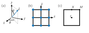
Figure 1: (Color online) Geometry of the dipolar Heisenberg model on square lattice. There is one polar molecule localized on each site of the square lattice within the $xy$ plane (b). Each molecule carries pseudo-spin 1/2. Their dipole moments are aligned along a common direction $\hat{d}$ specified by the polar angle $\theta$ and azimuthal angle $\phi$ (a). The Brillouin zone and selected high symmetry points are shown in (c).

The dipolar Heisenberg model may appear foreign and artificial from a solid state perspective. However, it arises naturally in ultracold quantum gases of magnetic atoms and polar molecules. For example, as discussed in details in Refs. Yao et al., 2015; Zou et al., 2017; Hazzard et al., 2014; Gorshkov et al., 2011, the pseudo-spin 1/2 describes two rotational states of the polar molecules such as KRb confined in a deep optical lattice, the spin exchange is mediated by the dipole-dipole interaction between the molecules, Eq. (3), and $\hat{d}$ is the direction of all the dipoles along an external electric field. Experiments have successfully realized the dipolar Heisenberg model on cubic optical lattice and measured its spin dynamics Yan et al. (2013); Bohn et al. (2017). We note that similar spin models with long range interactions can also be realized using cold atoms with large magnetic moments de Paz et al. (2013), atoms in the highly excited Rydberg states Schauß et al. (2012); Labuhn et al. (2016), and trapped ionsBritton et al. (2012); Islam et al. (2013).

Previously, Zou, Liu and one of us solved $H_{\hat{d}}$ on square lattice by using the tensor network ansatz and keeping only the nearest and next nearest exchange couplings Zou et al. (2017). They found evidence for a quantum paramagnetic phase, likely a spin liquid, sandwiched between the Néel and stripe phase. The ansatz employed an $L\times L$ unit cell with periodic boundary conditions. It was unable to go beyond $\phi\sim 20^{\circ}$, because the small cluster cannot accommodate the incommensurate spiral order which becomes relevant at these higher $\phi$ values. Thus, a full phase diagram of $H_{\hat{d}}$ from tensor networks is still lacking. To get a better understanding of the model, an independent method is needed. First, the method should be able to take into account the long range interactions faithfully and avoid severe truncations in the interaction range. Second, it should work directly with infinite lattice in the thermodynamic limit to accurately describe the spiral oder to predict the phase diagram for all values of $\theta$ and $\phi$. Third, it should go beyond the leading order spin wave theory Zou et al. (2017) or random phase approximation by treating all instabilities on same footing without bias.

In this paper, we adopt a method that satisfy these three requirements above. We obtain the zero temperature (ground state) phase diagram of $H_{\hat{d}}$ using the pseudo-fermion functional renormalization group analysis. We show that the dipolar Heisenberg model shows, besides the Néel, stripe and spiral phases, an extended quantum paramagnetic region where long range order is suppressed from $\phi=0^{\circ}$ all the way up to $\phi=45^{\circ}$. This observation is in broad agreement with previous results from different methods. It is also in line with recent theoretical evidence of spin liquid phase for the dipolar Heisenberg model on the triangular lattice Yao et al. (2015); Keles and Zhao (2018).

The rest of the paper is organized as follows: In Sec. II we present details of the pseudo-fermion functional renormalization group. In Sec. II.1, we outline the renormalization flow equations for the single particle self-energy and two particle vertex in a compact form. In Sec. II.2, we introduce the necessary parametrizations of the two particle vertex that exploits the symmetries of our problem to make the numerical solution feasible. In Sec. II.3, we provide details of our numerical implementation. In Sec. III, we present our main results on the dipolar Heisenberg model model including the phase diagram and the FRG flows for representative points in each phase. The long range ordered phases and the quantum paramagnetic phase are discussed in separate subsections. Finally, we summarize our main observations in Sec. IV and discuss their experimental implications.

II Pseudo-fermion Functional renormalization group

To tackle the many-body spin problem of $H_{\hat{d}}$ in Eq. (2), we first recast it in a fermionic representation by using

$$\mathbf{S}_{i}=\frac{1}{2}\boldsymbol{\sigma}_{\alpha^{\prime}\alpha}\psi^{\dagger}_{\alpha^{\prime}i}\psi_{\alpha i}$$ (5)

similar to the parton construction used in the study of frustrated quantum magnets and sometimes referred to as the Abrikosov fermion representation. Here $\psi$’s are anti-commuting fermion field operators and $\sigma$’s are the usual spin-1/2 Pauli matrices. After the substitution, the Hamiltonian $H_{\hat{d}}$ becomes

$$H[\bar{\psi},\psi]=\sum_{i_{1}i_{2}}\frac{J_{i_{1}i_{2}}}{4}\boldsymbol{\sigma}_{\alpha_{1}^{\prime}\alpha_{1}}\cdot\boldsymbol{\sigma}_{\alpha_{2}^{\prime}\alpha_{2}}\psi^{\dagger}_{\alpha_{1}^{\prime}i_{1}}\psi^{\dagger}_{\alpha_{2}^{\prime}i_{2}}\psi_{\alpha_{2}i_{2}}\psi_{\alpha_{1}i_{1}}.$$ (6)

We will drop the subscript $\hat{d}$ for $H$ in the rest of the paper for brevity. This Hamiltonian for fermions has quartic spin-dependent interactions but no hopping between sites. Thus the bare single-particle Green function is only frequency dependent (the chemical potential is kept at zero throughout the calculation)

$$G^{(0)}(\omega)=\frac{1}{i\omega}$$ (7)

which comes from imaginary time derivative term in the action $S[\bar{\psi},\psi]=\bar{\psi}\partial_{\tau}\psi+H[\bar{\psi},\psi]$. The translation of the spin problem to a fermion problem enables one to use the well-established many-body techniques for correlated electrons to understand the ground state of the system. Note, however, that the fermion problem Eq. (6) is very peculiar: the interaction energy is much larger (in fact infinitely larger) than the kinetic energy. For this reason, we resort to functional renormalization group which is capable of describing such strongly interacting models Metzner et al. (2012); Kopietz et al. (2010).

Functional renormalization group (FRG) is an elegant theoretical framework that implements the Wilsonian scale transformation in a systematic way to integrate out the high energy degrees of freedom and obtain a low energy effective field theory. There are several alternative functional renormalization techniques suitable for the Hamiltonian in Eq. (6). Here, our main goal is to provide an impartial diagnosis of competing phases and the many-body instabilities at low energies. To this end, we employ a purely fermionic FRG scheme without auxiliary Hubbard-Stratanovich fields. This approach is known as pseudo-fermion functional renormalization group (pf-FRG) Reuther and Wölfle (2010) and it is proven successful in identifying spin liquid behavior in a variety of models Reuther and Wölfle (2010); Reuther and Thomale (2011); Reuther et al. (2011, 2014); Buessen and Trebst (2016); Iqbal et al. (2016).

II.1 Flow Equations

The starting point of pf-FRG is the fermionic renormalization flow equation derived from vertex expansion up to one loop order:

$$\frac{d}{d\Lambda}\Sigma(\omega_{1}) =-\sum_{2}\Gamma_{1,2;1,2}S(\omega_{2}),$$ (8)

$$\frac{d}{d\Lambda}\Gamma_{1^{\prime},2^{\prime};1,2} =\sum_{3,4}\Pi(\omega_{3},\omega_{4})\biggr{[}\frac{1}{2}\Gamma_{1^{\prime},2^{\prime};3,4}\Gamma_{3,4;1,2}$$

$$-\Gamma_{1^{\prime},4;1,3}\Gamma_{3,2^{\prime};4,2}+\Gamma_{2^{\prime},4;1,3}\Gamma_{3,1^{\prime};4,2}\biggr{]},$$ (9)

where we leave scale ($\Lambda$) dependence implicit in the self energy $\Sigma$, the two particle vertex $\Gamma$, the full propagator $G$, and the single-scale propagator $S$ for brevity. The subscripts are shorthand notation, for example,

$$\Gamma_{1^{\prime},2^{\prime};1,2}\equiv\Gamma(i_{1}^{\prime},\alpha_{1}^{\prime},\omega_{1}^{\prime},i_{2}^{\prime},\alpha_{2}^{\prime},\omega_{2}^{\prime};i_{1},\alpha_{1},\omega_{1},i_{2},\alpha_{2},\omega_{2})$$

with site index $i$, spin $\alpha$, and frequency $\omega$ (we only consider zero temperature so the Matsubara frequency becomes continuous variable). The summation denotes integration over continuous frequencies and summation over lattice sites and spin. The two scale-dependent propagators defined by $G(i^{\prime},\omega^{\prime},\alpha^{\prime};i,\omega,\alpha)=\delta_{i^{\prime}i}\delta_{\omega,\omega^{\prime}}\delta_{\alpha^{\prime},\alpha}G(\omega)$ and $S(i^{\prime},\omega^{\prime},\alpha^{\prime};i,\omega,\alpha)=\delta_{i^{\prime}i}\delta_{\omega,\omega^{\prime}}\delta_{\alpha^{\prime},\alpha}S(\omega)$ are diagonal in site, spin and frequency space at all stages of renormalization where

$$G(\omega)=\frac{\Theta(|\omega|-\Lambda)}{i\omega+\Sigma(\omega)},\quad S(\omega)=\frac{\delta(|\omega|-\Lambda)}{i\omega+\Sigma(\omega)},$$ (10)

and $\Sigma(\omega)$ is the self-energy. By using a diagrammatic expression for the vertex

$$\Gamma_{1^{\prime},2^{\prime},1,2}=\leavevmode\hbox to34.01pt{\vbox to25.18pt{\text{[drawing]}}},\\ 1 2 1^{\prime} 2^{\prime} 1 2 1^{\prime} 2^{\prime}$$

Eq. (9) can be represented diagrammatically by the familiar particle-particle, particle-hole and exchange channels as shown by the following one-loop diagrams:

$$\leavevmode\hbox to71.85pt{\vbox to34.97pt{\text{[drawing]}}}+\leavevmode\hbox to72.62pt{\vbox to34.97pt{\text{[drawing]}}}+\leavevmode\hbox to72.62pt{\vbox to34.97pt{\text{[drawing]}}} 1 2 1^{\prime} 2^{\prime} 3 4 1 1^{\prime} 2 2^{\prime} 3 4 1 2^{\prime} 2 1^{\prime} 3 4 1 2 1^{\prime} 2^{\prime} 3 4 1 1^{\prime} 2 2^{\prime} 3 4 1 2^{\prime} 2 1^{\prime} 3 4$$

Different from the usual practice of FRG applied to correlated electrons Kopietz et al. (2010), pf-FRG uses a modified expression for the product of Green functions (polarization bubbles) by using the following full derivative

$$\Pi(\omega_{3},\omega_{4})=-\frac{d}{d\Lambda}\left[G(\omega_{3})G(\omega_{4})\right].$$ (11)

which includes terms beyond one-loop expansion Katanin (2004).

The expressions given in Eq. (8) and (9) forms a non-linear integro-differential system of equations, with the initial condition defined by the bare Hamiltonian $H_{\hat{d}}$ at the ultraviolet (UV) scale ($\Lambda_{\mathrm{UV}}\rightarrow\infty$) such that

$$\Sigma(\omega)\big{|}_{\Lambda=\Lambda_{\mathrm{UV}}} =0,$$ (12)

$$\Gamma_{1,2;1^{\prime},2^{\prime}}\big{|}_{\Lambda=\Lambda_{\mathrm{UV}}} =\mathcal{\hat{A}}\frac{1}{4}\sigma^{\mu}_{\alpha_{1}\alpha_{1}^{\prime}}\sigma^{\mu}_{\alpha_{2}\alpha_{2}^{\prime}}J_{i_{1},i_{2}}\delta_{i_{1}i_{1}^{\prime}}\delta_{i_{2}i_{2}^{\prime}}$$

where $\mathcal{\hat{A}}$ is the antisymmetrization operator. The flow equations for the two-particle vertex and the single particle self-energy describe ordering tendencies as the RG scale $\Lambda$ is systematically lowered from $\Lambda_{\mathrm{UV}}$.

II.2 Parametrization of the Vertex

To reduce the computational cost, we use the symmetries of the system such as spin $SU(2)$ invariance, translational invariance, and the lattice point group symmetry. These symmetries can be taken into account in an efficient way by using suitable parametrizations of the two particle vertex. For example, we perform the lattice parametrization by using

$$\Gamma_{1^{\prime},2^{\prime};1,2}=\mathcal{\hat{A}}\Gamma_{12}^{1^{\prime},2^{\prime},1,2}\delta_{i_{1}^{\prime}i_{1}}\delta_{i_{2}^{\prime}i_{2}}.$$ (13)

Here we have shortened the notation such that the lower indices stand for sites $i$ and the upper indices stand for the frequency and spin $(\omega,\alpha)$ as follows

$$\mathcal{O}_{12} \rightarrow\mathcal{O}(i_{1},i_{2})$$

$$\mathcal{O}^{1^{\prime},2^{\prime},1,2} \rightarrow\mathcal{O}(\alpha_{1}^{\prime},\omega_{1}^{\prime},\alpha_{2}^{\prime},\omega_{2}^{\prime},\alpha_{1},\omega_{1},\alpha_{2},\omega_{2}).$$ (14)

Note that full vertex $\Gamma_{1^{\prime},2;,1,2}$ is distinguished from the site-parametrized vertex $\Gamma_{12}^{1^{\prime},2^{\prime},1,2}$ by its arguments. The parametrization Eq. (13) can be expressed diagrammatically

$$\leavevmode\hbox to33.24pt{\vbox to24.4pt{\text{[drawing]}}}=\delta_{i_{1}^{\prime}i_{1}}\delta_{i_{2}^{\prime}i_{2}}\leavevmode\hbox to42.26pt{\vbox to35.79pt{\text{[drawing]}}}-\delta_{i_{1}^{\prime}i_{2}}\delta_{i_{2}^{\prime}i_{1}}\leavevmode\hbox to42.26pt{\vbox to35.79pt{\text{[drawing]}}} 1 2 1 2 i_{1} i_{2} 1 2 1^{\prime} 2^{\prime} i_{1} i_{2} 1 2 2^{\prime} 1^{\prime} 1 2 1 2 i_{1} i_{2} 1 2 1^{\prime} 2^{\prime} i_{1} i_{2} 1 2 2^{\prime} 1^{\prime}$$

where the site parametrized vertex is depicted by a zigzag line. After substitution of Eq. (13) in the flow equation (9) and equating the terms associated with $\delta_{i_{1}^{\prime}i_{1}}\delta_{i_{2}^{\prime}i_{2}}$ and $\delta_{i_{1}^{\prime}i_{2}}\delta_{i_{2}^{\prime}i_{1}}$ separately we find

$$\frac{d}{d\Lambda}\Gamma_{12}^{1^{\prime}2^{\prime}12}=\sum_{\omega_{3}\alpha_{3},\omega_{4}\alpha_{4}}\Pi(\omega_{3},\omega_{4})\biggr{[}\underbrace{\Gamma_{12}^{1^{\prime}2^{\prime}34}\Gamma_{12}^{3412}}_{\leavevmode\hbox to45.92pt{\vbox to23.56pt{\text{[drawing]}}}}-\underbrace{\sum_{i_{3}}\Gamma_{13}^{1^{\prime}413}\Gamma_{32}^{32^{\prime}42}}_{\leavevmode\hbox to45.92pt{\vbox to23.56pt{\text{[drawing]}}}}+\underbrace{\Gamma_{12}^{1^{\prime}413}\Gamma_{22}^{32^{\prime}24}}_{\leavevmode\hbox to45.92pt{\vbox to23.56pt{\text{[drawing]}}}}+\underbrace{\Gamma_{11}^{1^{\prime}431}\Gamma_{12}^{32^{\prime}42}}_{\leavevmode\hbox to45.92pt{\vbox to24.42pt{\text{[drawing]}}}}+\underbrace{\Gamma_{12}^{42^{\prime}13}\Gamma_{12}^{1^{\prime}342}}_{\leavevmode\hbox to45.92pt{\vbox to23.79pt{\text{[drawing]}}}}\biggr{]}$$ (15)

where the diagrammatic expression of each term is presented below an underbrace. These five diagrams are well known in many-body theory: the first term is the particle-particle ladder whereas the last diagram is the particle-hole ladder. The third and fourth diagrams are vertex corrections. The second diagram is the RPA bubble. A key strength of the pf-FRG approach is that the parametrization of the two particle vertex Eq. (13) along with the full propagators Eq. (10) enforces exactly one fermion per site throughout the flow. This ensures that Eq. (5) is a faithful representation of the original spin problem (empty or double occupation of any site is strictly forbidden). The preservation of fermion number constraint within pf-FRG has been numerically demonstrated in Ref. Buessen et al., 2018a (see also Ref. Reuther and Wölfle, 2010 for more details).

Finally, we use the following spin parametrization for systems with $SU(2)$ symmetry

$$\Gamma_{12}^{1^{\prime}2^{\prime}12} =\Gamma_{i_{1}i_{2}}^{\mathrm{spin}}(\omega_{1}^{\prime},\omega_{2}^{\prime},\omega_{1},\omega_{2})\boldsymbol{\sigma}_{\alpha_{1}^{\prime}\alpha_{1}}\cdot\boldsymbol{\sigma}_{\alpha_{2}^{\prime}\alpha_{2}}$$

$$+\Gamma_{i_{1}i_{2}}^{\mathrm{dens}}(\omega_{1}^{\prime},\omega_{2}^{\prime},\omega_{1},\omega_{2})\delta_{\alpha_{1}^{\prime}\alpha_{1}}\delta_{\alpha_{2}^{\prime}\alpha_{2}}.$$ (16)

This leads to two distinct sets of coupled flow equations for $\Gamma^{\mathrm{spin}}$ in the spin channel and $\Gamma^{\mathrm{dens}}$ in the density channel. The resulting equations are rather lengthy and can be found in Ref. Reuther and Wölfle, 2010. The vertex functions are expressed in terms of Mandelstam variables $s=\omega_{1}+\omega_{2}=\omega_{1}^{\prime}+\omega_{2}^{\prime}$, $t=\omega_{1}-\omega_{3}$, $u=\omega_{1}-\omega_{4}$ by a change of variable. These variables efficiently encode the symmetries in frequency space such as frequency conservation $\omega_{1}+\omega_{2}=\omega_{1}^{\prime}+\omega_{2}^{\prime}$. We also exploit the reflection symmetry with respect to the plane containing the dipole direction $\hat{d}$ and perpendicular to the square lattice. Note that the $C_{4}$ rotational symmetry is broken once the dipoles are tilted, $\theta\neq 0$.

II.3 Numerical Implementation

Translational invariance implies that the vertex functions $\Gamma_{i_{1}i_{2}}$ only depend on the distance between sites $i_{1}$ and $i_{2}$. In our numerics, we use the translational invariance to fix $i_{1}$ as a reference site and consider all $\Gamma_{i_{1}i_{2}}^{\mathrm{spin}}$ and $\Gamma_{i_{1}i_{2}}^{\mathrm{dens}}$ with $i_{2}$ within an $N_{L}\times N_{L}$ square region centered at $i_{1}$. Formally this scheme corresponds to an infinite system with finite truncation of interaction range. (In the pf-FRG literature, this is sometimes referred as “the cluster size” for brevity.) The frequency $\omega$ is discretized and lives on a logarithmic frequency grid of $N_{\omega}$ points from a very large ultraviolet scale $\Lambda_{\mathrm{UV}}$, down to a very small infrared scale $\Lambda_{\mathrm{IR}}$. Since the only energy scale of the problem is the dipolar exchange $J_{0}=1$, the small and large energy cutoffs should satisfy $\Lambda_{\mathrm{UV}}\gg 1$ and $\Lambda_{\mathrm{IR}}\ll 1$, respectively. We slowly reduce the RG scale $\Lambda$ all the way from the ultraviolet to the infrared with four steps between two consecutive frequencies on the grid. This gives $N_{\Lambda}=4N_{\omega}$ renormalization steps in total. We solve the first order coupled flow equations (8)-(9) with the initial condition (12) for the dipolar Heisenberg model (2) on the multidimensional grid of lattice sites and frequencies described above using the fourth order Runge-Kutta algorithm. The overall computational cost of the numerical solution scales with $N_{\Lambda}\cdot N_{L}^{2}\cdot N_{\omega}^{4}$. We perform simulations for lattice sizes up to $N_{L}=11$ and $N_{\omega}=64$ frequencies and for $N_{\Lambda}$ that takes up to 8 renormalization steps between neighboring frequencies. We checked that increasing these parameters does not change our results significantly for several selected points in the phase diagram. Our code is written in Python to run on Graphical Processing Units (GPU) with massive parallelism implemented by using the open source Numba compiler. As an example, for the system sizes mentioned above, a single simulation for a given set of parameters takes about 4.5 hours in a state-of-the-art GPU such as NVIDIA TITAN Xp with 3840 cuda cores.

Typically, there are about 20-30 million running couplings ($\Gamma$’s) being monitored during each step of the FRG flow. Analysis of such a large collection of coupling constants is facilitated by the calculation of certain two particle correlation functions. At each RG scale, the single-particle self-energy and the two-particle interaction vertex can be used to obtain the static spin susceptibility in real space using

$$\chi_{i_{1},i_{2}} = \int_{0}^{\infty}d\tau\langle TS_{i_{1}}(\tau)S_{i_{2}}(0)\rangle$$

$$= \leavevmode\hbox to163.38pt{\vbox to24.41pt{\text{[drawing]}}}, + +$$

where “” is the diagrammatic representation for the Pauli matrix $\sigma$, related to the spin at site $i$ by $S_{i}=1/2\sigma_{\alpha^{\prime}\alpha}\psi^{\dagger}_{\alpha^{\prime}i}\psi_{\alpha i}$. After Fourier transforming to the momentum space, the spin susceptibility $\chi(\mathbf{p})$ gives clues to the leading ordering instabilities, if any, as the renormalization flow approaches the infrared scale. For example, the locations of the susceptibility maxima $\chi_{\mathrm{max}}$ in the Brillouin zone determine the ordering wave vector for the incipient long range order. Typically $\chi_{\mathrm{max}}$ displays a Curie-Weiss-like behavior at large RG scales $\Lambda\gg 1$. The effects of quantum correlations start to emerge around $\Lambda\approx 1$. If there is an instability toward long ranged order, below a critical scale $\Lambda_{c}<1$, the susceptibility shows rapid increase until the flow breaks down and is replaced with unphysical jumps. On the other hand, the susceptibility may continuously flow to lowest numerical renormalization scale $\Lambda\rightarrow\Lambda_{\mathrm{IR}}$. This points to a quantum paramagnetic phase such as a spin liquid. Examples of these different flow behaviors will be given below.

III Phase diagram from FRG

Before discussing the full FRG results, we first review the classical limit of the dipolar Heisenberg model on square lattice, previously discussed in Ref. Zou et al., 2017. The classical phase diagram contains three phases schematically shown in Fig. 2. The Néel order is stabilized for small values of $\theta$. It gives way to the stripe order at large $\theta$ if $\phi$ is not too large. For large $\phi$ close to $45^{\circ}$ and large $\theta$, the system is in the spiral phase. FRG provides an elegant way to obtain the classical phase diagram via the solution of the flow equations by ignoring all frequency dependences. This method has been shown to be consistent with random phase approximation and Luttinger-Tisza method Baez and Reuther (2017). It also serves as a useful benchmark for FRG. Specifically, we start from the UV scale with the initial condition Eq. (12) and numerically monitor the flows of the frequency-independent vertices under the sliding renormalization scale $\Lambda$. When the absolute maximum of the vertex reaches a large cutoff value, a divergence is detected and we stop the flow. The scale at which this cutoff value is reached gives us the critical ordering scale $\Lambda_{c}$, which can be interpreted roughly as an estimation of the critical temperature. The corresponding classical order is found by Fourier transforming the susceptibility and examining the location of its peaks.

The resulting critical scales are shown in false color in the top row of Fig. 3. Here the color yellow (blue) indicates high (low) values of the critical scale $\Lambda_{c}$. The contour lines give a rough guide for the phase boundaries (not shown explicitly to avoid clutter). The three classical phases show up as three plateaus of $\Lambda_{c}$ in the parameter space of the $\theta-\phi$ plane. For the antiferromagnetic Néel order at small dipolar tilting $\theta$, the susceptibility shows four maxima at the corners of the Brillouin zone (the $M$-point, see Fig. 1). As $\theta$ is increased, peaks at the corners of the Brillouin zone start to extend and eventually merge at the $X$-point. For larger $\theta$, the susceptibility peak moves to the $X$-point, indicating the stripe order. With $\theta$ fixed but increasing the azimuthal angle $\phi$ beyond a critical value, the peaks at the $X$ points start moving towards the $\Gamma$ point, the center of the Brillouin zone, indicating the spiral order. From Fig. 3, we see that the stripe order typically has large critical scales whereas $\Lambda_{c}$ is suppressed close to the Néel-stripe phase boundary. The suppression is most severe near a region around $\theta\sim\phi\sim 45^{\circ}$. In the next subsection, we analyze the FRG flow equations with full frequency dependence. Special attention will be given to regions where the long range orders are suppressed.

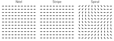
Figure 2: Spin configurations for the Néel, stripe and spiral order. These are the three competing classical long-range orders for the dipolar Heisenberg model on square lattice.

III.1 Three long-range ordered phases

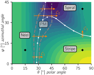
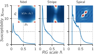
Figure 3: (Color online) Phase diagram of dipolar Heisenberg model on square lattice as function of dipole tilting angles $\theta$ and $\phi$. Three long-range orders are Néel, stripe and spiral phases. Color contours are critical RG scales of obtained from frequency independent FRG. For three selected points (black diamonds) in the phase diagram, the flows of maximum susceptibility are shown in the lower panel. The corresponding susceptibility profiles throughout the Brillouin zone at a small RG scale are shown as the insets of the lower panel. The orange arrows denoted by $\mathcal{C}_{1}$, $\mathcal{C}_{2}$ and $\mathcal{C}_{3}$ are cuts near the phase boundaries. The dashed lines indicate the estimated boundary of a quantum paramagnetic (PM) phase.

The main results of our full FRG calculations are summarized in Fig. 3. We systematically perform multiple cuts through the $\theta-\phi$ plane and examined the spin susceptibility profiles in the momentum space in conjunction with the renormalization flow of $\chi_{\mathrm{max}}$ to determine the many-body ground state. The resulting phase boundaries are shown in Fig. 3 with white lines, overlaid on top of the false color $\Lambda_{c}$ obtained from frequency independent FRG discussed above. The lower panel shows the RG flows of $\chi_{\mathrm{max}}$ for a selected point from each phase. The insets show the corresponding susceptibility profiles within the Brillouin zone. The region between the grey dashed lines in the vicinity of the phase boundaries is another phase and it will be described separately in the next subsection.

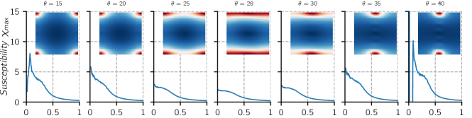
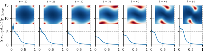
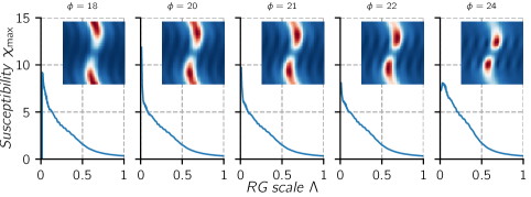
Figure 4: (Color online) Renormalization group flows of maximum susceptibility $\chi_{\mathrm{max}}$ along three cuts in the vicinity of the phase boundaries. Top row is the $\mathcal{C}_{1}$ cut from the Néel phase to stripe phase, middle row is the $\mathcal{C}_{2}$ cut from the Néel phase to spiral phase and the bottom row is the $\mathcal{C}_{3}$ cut from the stripe to spiral phase. Insets show the susceptibility profiles near the end of each flow. Within an extended window of angle $\theta$ (top and middle row), the susceptibility flows smoothly down to $\Lambda\rightarrow 0$ and shows no sign of divergence or breakdown. This points to a paramagnetic ground state.

The full FRG predicts three long range ordered phases. We can understand each phase by selecting a representative point (the black diamonds in Fig. 3) in the phase diagram and inspecting its numerical FRG data. Let us start with $\theta=15^{\circ}$ and $\phi=10^{\circ}$, a point deep inside the Néel phase. The spin susceptibility profile $\chi(\mathbf{p})$ over the full Brillouin zone at a small RG scale $\Lambda\approx 0.4$ (shown in the inset of lower panel) clearly indicates the leading spin correlations are of Néel type because of the peaks at the corners of the Brillouin zone. However, the peak position by itself is not sufficient to identify the presence of a complete instability. The susceptibility data as a function of the RG scale should also be inspected. To this end, we focus on $\chi_{\mathrm{max}}$ at the peak position, the $M$-point. Its renormalization flow is shown in the lower panel of Fig. 3. Here, as $\Lambda$ is gradually reduced, we first observe an upturn followed a shoulder with tiny oscillations around $\Lambda\sim 0.2-0.3$. These oscillations are due to the discretization in the frequency grid. They are well controlled, and can be reduced by using a finer grid. Upon further decreasing $\Lambda$, a steep increase of the susceptibility is observed indicating a divergence being developed. Shortly afterward, however, the continuous flow breaks down and is replaced by unphysical, discontinuous evolution of $\chi$ (not shown for lower values of $\Lambda$). The breakdown of smooth pf-FRG flow is in a large part due to the finite truncation $N_{L}$ of the effective interaction range in our numerical implementation. The truncation regulates the divergence and eventually leads to unphysical flows at low $\Lambda$. A faithful description of the divergence would require diverging correlation length, i.e. ever increasing $N_{L}$. Even though a true divergence is hard to reach in finite $N_{L}$ implementation of pf-FRG, one can make sure the flow indeed suggests long range order by systematically varying $N_{L}$. In practice, the breakdown of the continuous flow is a clear indication of incipient long range order in pf-FRG provided that $N_{L}$ is sufficiently large (see Ref. Reuther and Wölfle, 2010 and Ref. Keles and Zhao, 2018 for a detailed discussion).

Similar results are shown in Fig. 3 for two points deep inside the stripe and spiral phases respectively. For the stripe phase at $\theta=80^{\circ}$, $\phi=10^{\circ}$, the susceptibility peak is at the $X$-point signaling the alternating layered structure shown in the middle panel of Fig. 2. The spiral phase at $\theta=80^{\circ}$, $\phi=40^{\circ}$ has an ordering wave vector corresponding to the incommensurate spin texture as shown in the right panel of Fig. 2. Note that the susceptibilities flow up to much larger values in the stripe and spiral phases in compared to the Néel phase, since the selected points in these phases are further away from the phase boundary.

We can determine the boundary between these long range ordered phases by tracking the peak positions of the susceptibility. Because the peak becomes broadened near the phase boundaries, it is much easier to monitor the degeneracy of $\chi_{\mathrm{max}}$ and define the phase boundary as where it is most degenerate, i.e., the peak is most smeared and extended. This yields the dotted and solid white lines in Fig. 3. One can check these lines are exactly where the peak position changes qualitatively, for example, from peak at $M$ (Néel order) to peak at $X$ (stripe order). The solid white line gives an accurate phase boundary between the stripe and the spiral phase. On the other hand, we emphasize that the dotted white line separating the Néel and stripe/spiral phase is not the physical phase boundary. In the next subsection, we show that an extended quantum paramagnetic phase is sandwiched between these phases.

III.2 A robust quantum paramagnetic region

Now we show that within a rather broad region near the Néel-stripe and the Néel-spiral phase boundary, enclosed by the dashed lines in Fig. 3, long range order is suppressed, and the spin susceptibility flows smoothly and continuously down to the lowest RG scale $\Lambda_{\mathrm{IR}}$ without any indication of a divergence being developed. Thus the ground state within this region is a quantum paramagnet according to the FRG. The quantum paramagnetic region spans a width of about $5^{\circ}$ to $15^{\circ}$ in the $\theta$ direction, and persists to all $\phi$ values.

To demonstrate the paramagnetic behavior in the vicinity of the phase boundary, we take several cuts indicated by the orange arrows in Fig. 3. The detailed FRG flows are shown in Fig. 4 for three typical cuts labeled by $\mathcal{C}_{1}$ to $\mathcal{C}_{3}$. Among these, $\mathcal{C}_{1}$ is a cut from the Néel phase going into the stripe phase at $\phi=5^{\circ}$, $\mathcal{C}_{2}$ is a cut from the Néel phase to the spiral phase at $\phi=35^{\circ}$, and $\mathcal{C}_{3}$ is a cut from the stripe to the spiral phase with fixed $\theta=80^{\circ}$ but increasing $\phi$. Along the $\mathcal{C}_{1}$ cut (top row of Fig. 4), the flow pattern in the beginning (e.g. $\theta=15^{\circ}$) clearly indicates a long range Néel order. As we increase the dipolar tilting $\theta$, the sharp peaks at $M$ become broadened and extend towards each other along the $MX$ line. At the same time, the development of divergence in the maximum susceptibility $\chi_{\mathrm{max}}$ at low $\Lambda$ is gradually weakened. At $\theta=28^{\circ}$, the peak at $M$ is no longer visible. The spin susceptibility reaches maximum along the entire line connecting $M$ and $X$. Here, the RG flow of $\chi_{\mathrm{max}}$ remains remarkably smooth down to lowest numerical RG scale without any sign of instability, see the top row, middle panel of Fig. 4. With further increase in $\theta$, the susceptibility develops a new peak at $X$, and the flow of $\chi_{\mathrm{max}}$ becomes divergent at low $\Lambda$ again, signaling the stripe order. The width of the quantum paramagnetic region is estimated to be about $5^{\circ}$ for the $\mathcal{C}_{1}$ cut. The rough boundary of the paramagnetic region is indicated by the orange square bracket markers in Fig. 3.

The $\mathcal{C}_{2}$ cut (the middle row of Fig. 4) also reveals a similar quantum paramagnetic region. But this time, the region is significantly larger, within a window about $15^{\circ}$ wide (see the orange bracket in Fig. 3). Another cut above $\mathcal{C}_{2}$ indicates that the paramagnetic region narrows down at larger $\phi$ values. So the maximum quantum paramagnetic region is located where all three phases meet, around the $\mathcal{C}_{2}$ cut.

We also checked whether any quantum paramagnetic behavior persists near the stripe to spiral phase boundary. The $\mathcal{C}_{3}$ cut (bottom row of Fig. 4) reveals that the susceptibility flow in this region is markedly different compared to the $\mathcal{C}_{1}$ and $\mathcal{C}_{2}$ cuts. The flows indeed become smooth down to $\Lambda_{\mathrm{IR}}$ in a very narrow window of about $2^{\circ}$ in $\phi$, but they are not qualitatively different from nearby points along the cut. In particular, there is no clear suppression of susceptibility as observed in $\mathcal{C}_{1}$ and $\mathcal{C}_{2}$ cuts. Therefore, along along the $\mathcal{C}_{3}$ cut, a direct transition from stripe order to spiral order is observed, with no clear evidence for an intermediate paramagnetic phase with appreciable width.

III.3 Comparison with other methods

The same model $H_{\hat{d}}$ has been investigated previously using tensor network ansatz in Ref. Zou et al., 2017, where a quantum paramagnetic phase with a width of about 1 to 2 degrees was found for $\phi$ from $0^{\circ}$ up to $20^{\circ}$. Beyond $\phi\sim 20^{\circ}$, the tensor network algorithm becomes inaccurate due to the small cluster size which is incompatible with the spiral order. For this reason the phase boundary for $\phi>20^{\circ}$ is not known from the tensor algorithm. The dipolar Heisenberg model was also solved by spin wave analysis and Schwinger boson mean field (SBMF) theory in Ref. Zou et al., 2017. Both methods predicted a spin liquid region between the Néel and stripe phase for $\phi$ up to $\sim 35^{\circ}$, but the exact shape and position of the spin liquid phase are different. For example, SBMF yields a wider liquid region (the method is known to have the tendency of overestimating disordered phases). Finally we emphasize that in Ref. Zou et al., 2017, the exchange couplings $J_{ij}$ are truncated, i.e., only the nearest and next-nearest neighbor exchanges are retained.

The FRG approach adopted here is very different from these previous methods. For example, it does not work directly with variational wave functions or order parameter fields, and focuses instead on the correlation functions under the RG flow. Despite the difference, FRG also predicts a quantum paramagnetic region separating the Néel order and the stripe order, in broad agreement with Ref. Zou et al., 2017. Taken together, these numerical evidences consistently point to a quantum paramagnetic phase in the dipolar Heisenberg model on square lattice. The width of the paramagnetic region predicted from FRG is larger than that from tensor networks. We believe this is mainly due to that fact that longer range exchanges are kept in FRG, i.e. $J_{ij}$ for $|i-j|\leq N_{L}\gg 1$, which lead to stronger frustration and a more robust paramagnetic ground state compared to the $J_{1}$-$J_{2}$ model. It is also interesting to compare FRG with the modified spin wave theory which contains the leading terms in the $1/S$ expansion, as well as SBMF which can be related to the large $N$ limit of $Sp(N)$ spin models. The perturbative diagrammatic expansions in the three methods are rather different. The detailed analysis of FRG for spin-$S$ and $SU(N)$ spin models can be found in Refs. Baez and Reuther, 2017; Buessen et al., 2018b.

The new insight from our FRG calculation is that the paramagnetic region will persist to higher $\phi$ values, all the way to $\phi=45^{\circ}$. FRG works with infinite lattice and a large cutoff $N_{L}$ of the effective interaction range, and therefore is much better equipped to describe the spiral order. Near the classical Néel-spiral phase boundary, both orders are very weak with the critical temperature $T_{c}$ significantly suppressed (see for example the dark region in the top row of Fig. 3). They are melted by quantum fluctuations to form a quantum paramagnetic ground state. It is challenging to precisely determine the phase boundary between the paramagnetic phase and the long range order phases in pf-FRG. The dashed lines in Fig. 3 are results of a conservative estimation, and the quantum paramagnetic phase may actually occupy a larger region in the phase diagram. We hope our results can stimulate further work with large scale numerics and different methods to shed more light on this intriguing region.

IV Conclusion

Our main result is that a quantum paramagnetic phase occupies an extended region in the phase diagram of $H_{\hat{d}}$ on square lattice thanks to the long-range anisotropic dipolar exchange. Recall that in the $J_{1}$-$J_{2}$ model, finite $J_{2}$ leads to exchange frustration, and magnetic order is suppressed for $J_{2}/J_{1}\sim 0.5$. Here longer range exchange couplings tend to amplify the frustration. And tilting the dipoles alone is sufficient to achieve the frustration needed for a quantum paramagnetic phase. Dipole tilting also break the four-fold rotational symmetry of $H_{\hat{d}}$ to favor the spiral order at large $\theta$ and $\phi$. The paramagnetic phase is most robust (i.e. has the largest expanse in parameter space) in regions where all three long orders meet and compete, near the $\mathcal{C}_{3}$ cut in Fig. 3. The melting of magnetic orders as a consequence of dipolar exchange coupling is a general phenomenon. It has also been demonstrated for $H_{\hat{d}}$ on the triangular lattice Yao et al. (2015); Keles and Zhao (2018) and kagome lattice Yao et al. (2015).

In conclusion, we have demonstrated via numerical functional renormalization group that the spin-1/2 dipolar Heisenberg model is an excellent candidate for studying frustrated magnetism and searching for quantum spin liquids. Such spin models with long range dipolar exchange has already been realized in experiments with ultracold KRb molecules in deep optical lattices, and the spin dynamics has been measured by microwave spectroscopy Yan et al. (2013). We hope further progress in cooling the molecular gases Wu et al. (2012) and obtaining lattice fillings close to unity Moses et al. (2015) can enable direct observation and measurement of the phase diagram of the dipolar Heisenberg model.