A new solar neutrino channel for grand-unification monopole searches

Abstract

We identify a previously untapped discovery channel for grand-unification monopoles, arising from their ability to catalyse the direct decay of protons into monoenergetic 459 MeV antineutrinos within the Sun. Previous analyses omit this possibility as it necessarily involves an electroweak suppression factor, and instead search for the unsuppressed 20-50 MeV neutrinos produced via two-stage proton decays. By accounting for the relative difference in interaction cross section and experimental background at typical neutrino detection experiments, we demonstrate that this new channel in fact possesses greater discovery potential. As a case in point, using 5326 live days of Super-Kamiokande exposure we find that $2\;\sigma$ ($3\;\sigma$) deviations in the 20-50 MeV channel are amplified to $3\;\sigma$ ($4.6\;\sigma$) deviations in the 459 MeV case. Exploiting correlations between these two channels may also offer even greater statistical power.

I Introduction

Arising naturally from the spontaneous breaking of non-Abelian symmetries, magnetic monopoles are arguably one of the most plausible facets of physics beyond the Standard Model. In particular, if the hypothesis of a grand unification of physical forces is indeed correct, then such phenomena are perhaps unavoidable.

Of course, despite their theoretical ubiquity magnetic monopoles also appear to be in short supply in our visible universe. Several decades of experimentation have yielded only a series of ever-tightening constraints Burdin et al. (2015), albeit with a few tantalising events which were later ruled out as monopole candidates Price et al. (1975); Cabrera (1982). Further efforts are ongoing, in particular at the MOEDAL experiment at the LHC Acharya et al. (2014).

Given the relatively inaccessible scale of grand unification to present-day particle physics, it is notable that remnant magnetic monopoles may conceivably provide the most accessible experimental signature available to our low-energy world. Another primary motivation for these efforts also lies in the success of the inflationary paradigm Ade et al. (2016), which suggests that any observation of superheavy magnetic monopoles is exceedingly unlikely. If found any topological relics of this nature would pose a very serious problem for inflationary theory, adding weight to their already huge experimental significance.

Furthermore, given their unusual properties it is also expected that even a single monopole can leave a highly distinctive signature, aiding any discovery efforts Pinfold et al. (2009). Indeed, of the possible monopole search strategies available to experimentalists, perhaps the most intriguing relies upon one particularly exotic property they possess. As originally established by Callan and Rubakov Callan (1982); Rubakov (1982), certain types of magnetic monopole are able to directly catalyse the decay of protons into positrons, without relying on superheavy gauge bosons or other intermediate states.

Since this leads to a cross-section lacking any of the usual supression factors, it is expected that these processes can occur at the rather rapid rates characteristic of the strong interaction. Furthermore, given the amount of energy liberated in such an event, it is then expected that it may have particularly noticeable effects in environments where we expect magnetic monopoles to accumulate, such as stellar interiors.

Naturally, there have been a number of studies oriented around these phenomena, in neutron stars Kolb et al. (1982), white dwarfs Freese and Krasteva (1999) and indeed our own Sun Arafune and Fukugita (1983). Further searches have also been performed looking for nucleon decays arising from the passage of magnetic monopoles through detector arrays Ambrosio et al. (2002); Aartsen et al. (2014, 2016).

However, as we will demonstrate in the following there has been also a subtle omission in the theoretical underpinning of some of these efforts, which has yet to be exploited. More specifically, whilst the resultant neutrinos offer a particularly useful hallmark of typical proton-decay processes, especially those occurring inside the Sun, existing searches focus entirely on two-stage processes such as $p\to\mu^{+}+K\to e^{+}+\nu_{e}+\overline{\nu}_{\mu}+X$. The resulting neutrino flux is mostly from $\pi^{+}$ Decay At Rest (DAR), which carries a characteristic energy ranging from $0$ to $52.8$ MeV, and peaking at $\sim 35\;\mathrm{MeV}$ Arafune and Fukugita (1983). It is also well known that protons cannot directly decay to neutrinos via GUT monopoles carrying only $SU(3)\otimes U(1)$ charge. That is to say, processes such as $p\to\pi^{+}+\overline{\nu}_{e}$ are apparently forbidden Ellis et al. (1982); Bais et al. (1983).

However, we note that at sufficiently short distances $SU(3)\otimes U(1)$ will be resolved to the (continuous) Standard Model group, $SU(3)\otimes SU(2)\otimes U(1)$. In this limit, the restrictions on processes like $p\to\pi^{+}+\overline{\nu}_{e}$ are no longer necessarily valid. Furthermore, even accounting for the electroweak suppression factor involved, the highly monoenergetic nature of the resulting antineutrino could in fact offer better discovery potential than is available via two-stage processes. Indeed, in this article we demonstrate precisely this via the following.

1. Grand-unification monopoles can catalyse the direct decay $p\to\overline{\nu}_{e}+\pi^{+}$, leading to an electroweak-suppressed monoenergetic 459 MeV antineutrino flux originating from the Sun.

2. Due to the reduced atmospheric neutrino background and increased interaction cross section at higher energies, the resulting significance of this signal at typical neutrino detection experiments can exceed that of the previously-explored low energy neutrino flux arising from unsuppressed monopole-induced proton decay.

The rest of this article is organised as follows. We briefly outline monopole catalysed proton decay processes in Section II, including the well-explored $p\rightarrow\mu^{+}+K$ process and our proposed $p\rightarrow\bar{\nu}_{e}+\pi^{+}$ process. We also estimate the solar monopole abundance as a preparation for the calculation of the neutrino flux. In Section III, we calculate the neutrino flux due to the two-stage proton decay (low energy) and the direct decay (459 MeV) signals. We also calculate the atmospheric neutrino flux based on Honda et al. (2015), in preparation for background estimation. In Section IV, we take Super-Kamiokande as an example and compute results for the three detection channels, namely scattering from electrons, protons, and oxygen nuclei. For the neutrino-nuclei cross section, we use the Fermi gas model only for the 459 MeV neutrinos, neglecting the low energy neutrino-oxygen scattering in line with Ref. Ueno et al. (2012). We also perform an energy cut to suppress the atmospheric neutrino background while keeping most of the signal events. In Section V, we compare the statistical significance of the two channels, and demonstrate that the new, high-energy channel possesses better discovery potential. In closing we briefly summarise our result, and indicate directions for future research.

II Monopole-induced proton decay

II.1 The Callan-Rubakov effect

As previously noted, one of the more interesting facets of monopole physics is the possibility of unsuppressed ‘exotic’ processes occurring, including those which may violate ordinarily conserved global symmetries. In practice there are several mutually compatible interpretations of how these phenomena can occur.

In one picture, we may imagine the monopole as being surrounded by a cloud of fermion condensate, polarising the vacuum. This is explicitly supported by the computation of matrix elements in a monopole background, giving $\langle\overline{\psi}_{L}\psi_{R}\rangle\sim 1/r^{3}$, where $r$ is the radial distance from the monopole core Rubakov (1982). Since monopoles couple with the inverse of the usual electromagnetic coupling, strong coupling phenomena of this nature should of course not be surprising. Incoming fermions are then able to scatter from this vacuum polarization, leading to processes $\psi_{L}+M\to\psi_{R}+M$.

Alternatively, toy models suggest that the dyon mode of the monopole may play a crucial role Polchinski (1984). Therein, charged fermions passing through the core of the monopole are absorbed, exciting the dyon mode. This excitation is unstable and so will subsequently decay into lighter charged fermions, allowing global symmetries to be violated.

A third, and far more heuristic perspective is to note that under S-duality, monopoles and superheavy gauge bosons are exchanged Montonen and Olive (1977). Disregarding the fact that this duality is likely inapplicable to the real world due to an absence of sufficient supersymmetry, this suggests that the usual process of proton decay via $X$ or $Y$ bosons may have a dual description in terms of proton scattering from a magnetic monopole, leading to the same conclusions.

In any case, we can keep in mind the diagrammatic logic of figure 1, where the monopole effectively supplies a baryon-number violating four-fermion vertex.

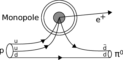
Figure 1: Heuristic diagram of monopole-induced proton decay. The monopole provides an effective baryon-number violating four-fermion vertex, allowing nucleons to decay. Figure reproduced from Aartsen et al. (2014).

For our purposes we will focus on the monopoles which arise in GUTs (Grand Unified Theories), and in particular the (equivalent) minimally-charged monopoles which occur in $SU(5)$ or $SO(10)$ theories. We note that in some models, such as Pati-Salam Chamseddine et al. (2013); Aydemir et al. (2016), there is no monopole catalysis of proton decay, and in others, such as flipped $SU(5)$, there are no monopoles whatsoever Dawson and Schellekens (1983).

Once this symmetry is fully broken down to the Standard Model gauge group, there will be monopoles left over from each symmetry breaking phase transition. We can specify each monopole up to gauge equivalence via the orientation it possesses within $SU(5)$, or more specifically by the embedding of the $SU(2)$ subgroup it defines. For $SU(3)\otimes SU(2)\otimes U(1)$ there are two choices for minimal monopoles, up to colour equivalence, given by the diag$(0,0,1,-1,0)$ and diag$(0,0,1,0,-1)$ embeddings Liu and Vachaspati (1997).

As we expect monopoles such as these accumulate within highly massive, long-lived objects such as our own Sun, the resultant high-energy neutrino flux from proton decay then offers a unique channel to infer their presence, and thereby test the grand-unification hypothesis.

II.2 Monopole-sourced two-stage solar neutrino production

In Refs. Dokos and Tomaras (1980); Lazarides and Shafi (1980); Bais et al. (1983), it is shown that monopoles that carry magnetic $U(1)$ charge $2\pi\;\mathrm{diag}(1/3,1/3,1/3,-1,0)$ and magnetic $SU(3)$ charge $2\pi\;\mathrm{diag}(-1/3,-1/3,2/3,0,0)$ can exist in the embedding of $SU(3)\otimes U(1)\subset SU(5)$. The magnetic $SU(5)$ charge before and after electroweak symmetry breaking is then $2\pi\;\mathrm{diag}(0,0,1,-1,0)$. It is straightforward to see that these monopoles carrying strictly $SU(3)\otimes U(1)$ charge cannot offer direct decay modes to a neutrino, since neutrinos have no electromagnetic or colour charge and are as such decoupled. To find the selection rules for processes allowed by these monopoles, we must construct the fermion doublets selected from the GUT multiplets via the ‘monopole’ $SU(2)$ subgroup. As demonstrated in Bais et al. (1983), neglecting phases these are

$$\begin{pmatrix}\overline{u}_{b}\\ u_{r}\end{pmatrix}_{L}\,,\quad\begin{pmatrix}d_{g}\\ e^{+}\end{pmatrix}_{L}\,,$$ (1)

and their conjugates. In line with the comments of the previous section, it is straightforward to recognise these as corresponding to the decay modes of an $SU(5)$ $X$ boson.

By contracting these doublets we can then construct the allowed operators in the monopole background, such as $(\overline{u}_{r}u_{b})(\overline{e}d_{g})$+h.c., which still conserve electric charge and $B-L$ quantum number. Computing these in a monopole background, we find no mass suppression factors, nor coupling constant dependence. As such, the corresponding proton decay cross section is expected to be purely geometric, and so dictated largely by the size of the proton Rubakov (1982).

Following Bais et al. (1983), we can then use these points to estimate the branching fraction of proton decays which produce neutrinos. The primary decay channel is $p\to e^{+}+\pi^{0}$, relative to which the dominant neutrino producing decay is $p\to\mu^{+}+K$ . Since these processes occur at geometric rates, it was argued therein that

$$\Gamma\left(p\to e^{+}\pi\right):\Gamma\left(p\to\mu^{+}K\right)\simeq 1:(m_{d}/m_{s})^{2}\,,$$ (2)

the overall scale of any individual catalysed process being set broadly by the Compton wavelengths of the particles involved. This ratio depends sensitively on the choice of quark masses, in that if we take their values from short-distance current algebra then $(m_{d}/m_{s})^{2}\sim 1/400$, whilst from their constituent masses $(m_{d}/m_{s})^{2}\sim 1/2$.

As with instantons, anomalous monopole-induced processes are tied to the presence of fermion zero modes. Indeed, we can identify the analog of the resulting ‘t Hooft vertex in Fig. 1. It is the bare mass appearing in the Lagrangian which is relevant for these zero modes, since they are defined at the level of the equations of motion. As in the instanton case this is then the mass appearing in their corresponding fermion determinants, and hence controlling the overall rate of these anomalous processes. Therefore, we use the short-distance current algebra mass in the rest of this article. Conversely, constituent masses are generally understood to arise from the large binding energy associated to the non-perturbative ‘gluing’ of free quarks into colour-neutral objects. In this context, they can only be expected to appear at higher orders in perturbation theory.

As with ordinary GUT proton decay, there is also a kinematic suppression to be accounted for. In this instance, assuming it is unchanged from the monopole-free context, this gives an additional factor of $\sim 1/2$. The resultant neutrino signal, peaked around 35 MeV Arafune and Fukugita (1983), then forms the basis for the most stringent present-day constraints on proton-decay induced solar neutrinos, by virtue of the Super-Kamiokande experiment Ueno et al. (2012).

II.3 Direct $\nu$-producing proton decay modes

It is firstly notable that in the context of proton decay within GUT theories there are a number of possible channels, some of which include direct decay of proton to a neutrino. Indeed, as explored in Sakai and Yanagida (1982) there are GUTs for which the dominant ‘ordinary’ decay mode is $p\to K^{+}+\nu$, rather than $p\to e^{+}+\pi^{0}$. Whilst this may not be possible directly in the monopole context, due to the relative rigidity of the Callan-Rubakov formalism, it is nonetheless suggestive that alternative channels of monopole-induced direct decays to neutrinos should be explored.

Let us then consider the minimal GUT monopoles lying in the embedding $SU(3)\otimes SU(2)\otimes U(1)\subset SU(5)$. There exist monopoles with the following magnetic charge.

$$U(1):\indent g_{1}h_{Y} =2\pi\;\mathrm{diag}\left(\frac{1}{3},\frac{1}{3},\frac{1}{3},-\frac{1}{2},-\frac{1}{2}\right),$$ (3)

$$SU(2):\indent g_{2}\sigma_{3} =2\pi\;\mathrm{diag}\left(0,0,0,\frac{1}{2},-\frac{1}{2}\right),$$ (4)

$$SU(3):\indent g_{3}\tau_{8} =2\pi\;\mathrm{diag}\left(-\frac{1}{3},-\frac{1}{3},\frac{2}{3},0,0\right),$$ (5)

where $g_{1},g_{2},g_{3}$ are the coupling constants of each gauge subgroup, $h_{Y}$ is the $U(1)$ hypercharge generator, and $\sigma_{3}(\tau_{8})$ is the (last) diagonal element of the Pauli (Gell-mann) matrices, respectively. The $SU(5)$ magnetic charge then reads $2\pi\;\mathrm{diag}(0,0,1,0,-1)$. We can again construct the doublets

$$\begin{pmatrix}e^{+}\\ u_{g}\end{pmatrix}_{L}\,,\quad\begin{pmatrix}\overline{d}_{r}\\ u_{b}\end{pmatrix}_{L}\,,\quad\begin{pmatrix}\overline{\nu}_{e}\\ d_{g}\end{pmatrix}_{L}\,,$$ (6)

and their conjugates, by acting on the $\overline{\textbf{5}}$ and 10 multiplets with the ‘monopole’ $SU(2)$ generator. It is straightforward to recognize the result as corresponding to the decay modes of an $SU(5)$ $Y$ boson.

Contracting as before we then find the effective four-fermion operator $(\overline{d}_{r}u_{b})(\overline{\nu}_{e}d_{g})+h.c.$, which allows $p\to\overline{\nu}_{e}+\pi^{+}$. Since this is a simple two-body decay, the resultant neutrino energy should be $\mathcal{O}(500)$ MeV. As a single stage decay involving only first generation fermions, it will also be the dominant neutrino production channel for $SU(3)\otimes SU(2)\otimes U(1)$ monopoles. Typically it should carry a 50% branching fraction, along with $p\to e^{+}+\pi^{0}$. The process $p\to\overline{\nu}_{\mu}+K^{+}$ is also possible, but again with a relative suppression factor of $(m_{d}/m_{s})^{2}$.

Since this process relies upon the electroweak component of the magnetic field, once electroweak symmetry is broken we can expect a characteristic suppression factor of $(m_{p}/m_{W})^{2}$ to enter, since the scale of ‘ordinary’ $SU(3)\otimes U(1)$ monopole-induced proton decay is expected to be set by the size of the proton. The resulting branching fraction for direct decays to neutrinos then becomes $\sim 10^{-4}$.

Although we can expect monopoles corresponding to both diag$(0,0,1,-1,0)$ and diag$(0,0,1,0,-1)$ embeddings to be produced around the GUT phase transition with roughly equal probability, a natural concern at this point is the stability of these latter relics under the electroweak phase transition. Indeed, it is suggested in Lazarides and Shafi (1980) that electroweak strings could form connecting these monopoles and their antimonopoles, leading to their rapid coannihilation. However, as argued in Gardner and Harvey (1984) it is also known that $\pi_{1}(SU(2)\otimes U(1)_{Y}/U(1))=0$, and so this does not seem mathematically plausible.

Another possibility is that these monopoles are ‘converted’ somehow during this phase transition into the $(0,0,1,-1,0)$ monopoles, and are hence absent at the present day Liu and Vachaspati (1997). However, there is no known mechanism to achieve this, and since these monopoles carry differing fractional electric charges such a process would naively appear to violate charge conservation.

A third possibility, discussed in Gardner and Harvey (1984); Vachaspati (1996), is just that the magnetic electroweak charge carried by these monopoles is screened below the electroweak scale. This is of course in line with the known screening of magnetic QCD charge below $\Lambda_{QCD}$. As then perhaps the most physically plausible of the three options, we will assume that this effect is in operation and proceed accordingly.

Since the only overall suppression we then expect is related to the scale at which the $SU(3)\otimes SU(2)\otimes U(1)$ structure of the monopole becomes apparent, the relative suppression factor for direct vs indirect decays to neutrinos should be $(m_{p}/m_{W})^{2}(m_{s}/m_{d})^{2}$. Using the short-distance current algebra values for the quark masses, this then suggests the relative rate of direct to indirect decays to neutrinos should be roughly $1/16$. As we will see in the next section, the relative reduction in neutrino backgrounds and increase in interaction cross section at 459 vs 35 MeV can be more than sufficient to overcome this deficit experimentally.

II.4 Monopole abundance in the Sun

To compute the expected high-energy neutrino flux at Earth-based detectors, we firstly need to account for the astrophysical monopole abundance. The primary constraint in that regard for $10^{16}$ GeV GUT monopoles comes from the Parker bound, which is based on the survival of galactic magnetic fields Parker (1970). This gives the galactic monopole flux constraint

$$F_{M}\lesssim 10^{-16}\mathrm{cm}{}^{-2}\mathrm{s}{}^{-1}\mathrm{sr}{}^{-1}\,.$$ (7)

We define the fraction of $F_{M}$ to the above bound as $\phi_{M}$. Stricter bounds are available from the catalysis of nucleon decays inside neutron stars, however these depend somewhat on the unknown physics of neutron star interiors Kolb et al. (1982). Furthermore, it has been suggested that coannihilation processes may in fact reduce these limits to the level of the Parker bound anyway Kuzmin and Rubakov (1983).

From the age and size of the Sun, we can then estimate the total number of captured monopoles over the solar lifetime. In general we need to account for the infalling velocity and corresponding energy loss inside the Sun to determine the fraction of monopoles captured. In Ref. Frieman et al. (1988) it is estimated that this ‘capture fraction’ of $10^{16}$ GeV GUT monopoles is approximately one, and the number of monopoles captured in the Sun is approximately $N_{M}\sim 10^{25}\phi_{M}$.

On they other hand, there exists the possibility that the total monopole number may be diminished by coannihilation processes. In this case, one estimates the number of captured monopoles being $N_{M}\sim 10^{17}(\phi_{M})^{1/3}$ Frieman et al. (1988). A considerable source of uncertainty here is related to the unknown nature of the magnetic field in the stellar interior, which could separate monopoles and antimonopoles, and thus prevent annihilation. Furthermore, if these processes do occur, the timescale associated to the annihilation process is largely unknown. In principle the monopole-antimonopole annihilation cross section should be set by the GUT scale, and their coannihilation may occur at rates which are negligible for our purposes .

In any case, we primarily aim to demonstrate that the 459 MeV monoenergetic antineutrino flux offers better discovery potential than the indirect decays previously explored in Ueno et al. (2012). Since coannihilation will affect both direct and indirect processes equally, it is not a relevant consideration for our purposes. Therefore, instead of a thorough and detailed classification of monopole physics, we take a phenomenological ‘bottom-up’ approach and neglect the coannihilation of monopoles for the rest of the analysis, along the same lines as Ref. Arafune and Fukugita (1983).

III Neutrino Flux

In this section we calculate the neutrino flux for both high and low energy signals, and the background, which mainly consists of atmospheric neutrinos. In order to estimate the number of events accurately, we take into account the neutrino oscillation effect in their propagation from the Sun to the Earth.

III.1 Signal Flux

III.1.1 459 MeV Neutrino

The energy production rate from nucleon decay is firstly

$$\frac{d\epsilon}{dt}=N_{M}\sigma\rho\beta c\,,$$ (8)

where $\rho$ is the average nucleon density, $\beta c$ is the thermal nucleon velocity at $T\sim 10^{7}\;\mathrm{K}\sim\mathcal{O}(\mathrm{keV})$, and $\sigma$ is the monopole-nucleon cross-section. It can be expressed as $\sigma=\sigma_{0}F(\beta)/\beta$, where $\sigma_{0}$ is a hadronic cross-section, and $F(\beta)$ is a nuclear form factor Arafune and Fukugita (1983). For hydrogen nuclei, $F(\beta)\simeq 0.17/\beta$. The neutrino emission rate and flux on Earth is then

$$F_{\overline{\nu}}\simeq\frac{1}{4\pi R^{2}}\frac{dN_{\overline{\nu}}}{dt}\,,\qquad\frac{dN_{\overline{\nu}}}{dt}=\frac{BR_{p\to\overline{\nu}}}{m_{p}c^{2}}\frac{d\epsilon}{dt}\,,$$ (9)

where $BR_{p\to\overline{\nu}}$ is the corresponding branching ratio and $R$ the average Earth-Sun distance. Since the $\mathcal{O}$(keV) thermal broadening can be largely neglected, we expect a monochromatic antineutrino flux

$$F_{\overline{\nu}}\sim\, 1.4\times 10^{4}\left(\frac{\sigma_{0}}{0.1\mathrm{mb}}\right)\left(\frac{\beta}{10^{-3}}\right)\left(\frac{BR_{p\to\overline{\nu}}}{10^{-4}}\right)\left(\frac{N_{M}}{10^{25}}\right)\,\mathrm{cm}{}^{-2}\mathrm{s}{}^{-1}\mathrm{sr}{}^{-1}\,,$$ (10)

of characteristic energy

$$E_{\overline{\nu}}=(m_{p}^{2}-m_{\pi^{+}}^{2})/2m_{p}=458.755\;\mathrm{MeV}\,.$$ (11)

Since different neutrino flavours interact differently, we need to account for the oscillation effects in their propagation from the Sun to the Earth.

$$P(\nu_{\alpha}\rightarrow\nu_{\alpha}) =1-4|U_{\alpha 2}|^{2}(1-|U_{\alpha 2}|^{2})\sin^{2}\frac{\Delta_{21}}{2}-4|U_{\alpha 3}|^{2}(1-|U_{\alpha 3}|^{2})\sin^{2}\frac{\Delta_{31}}{2}$$ (12)

$$\indent+2|U_{\alpha 2}|^{2}|U_{\alpha 3}|^{2}\left(4\sin^{2}\frac{\Delta_{21}}{2}\sin^{2}\frac{\Delta_{31}}{2}+\sin\Delta_{21}\sin\Delta_{31}\right)\,,$$ (13)

$$P(\nu_{\alpha}\rightarrow\nu_{\beta}) =4|U_{\alpha 2}|^{2}|U_{\beta 2}|^{2}\sin^{2}\frac{\Delta_{21}}{2}+4|U_{\alpha 3}|^{2}|U_{\beta 3}|^{2}\sin^{2}\frac{\Delta_{31}}{2}$$ (14)

$$~{}~{}+2\Re(U_{\alpha 3}^{*}U_{\beta 3}U_{\alpha 2}U_{\beta 2}^{*})\left(4\sin^{2}\frac{\Delta_{21}}{2}\sin^{2}\frac{\Delta_{31}}{2}+\sin\Delta_{21}\sin\Delta_{31}\right)$$ (15)

$$~{}~{}+4J_{(\alpha,\beta)}\left(\sigma^{2}\frac{\Delta_{21}}{2}\sin\Delta_{31}-\sin^{2}\frac{\Delta_{31}}{2}\sin\Delta_{21}\right),$$ (16)

where we use the same notation as Ref. Agarwalla et al. (2014), $\Delta_{ij}\equiv\delta m_{ij}^{2}L/2E=2.534\left(\frac{\delta m_{ij}^{2}}{\mathrm{eV}^{2}}\right)\left(\frac{\mathrm{GeV}}{E}\right)\left(\frac{L}{\mathrm{km}}\right)$, $J_{(\alpha,\beta)}$ is the Jarlskog invariant, $J_{(\alpha,\beta)}=\Im(U_{\alpha 1}^{*}U_{\beta 1}U_{\alpha 2}U^{*}_{\beta 2}$). Neglecting matter effects between the Earth and the Sun and using the average Earth-Sun distance $1.496\times 10^{8}\;\mathrm{km}$, the $\bar{\nu}_{\mu}\rightarrow\bar{\nu}_{e}$ appearance and $\bar{\nu}_{e}\rightarrow\bar{\nu}_{e}$ survival probability is

$$P(\bar{\nu}_{e}\rightarrow\bar{\nu}_{e}) \approx 0.38\,,$$ (17)

$$P(\bar{\nu}_{\mu}\rightarrow\bar{\nu}_{e}) \approx 0.47\,,$$ (18)

where we take $\delta_{CP}=0$. This gives us

$$F_{\overline{\nu}_{e}}\approx\, 5.3\times 10^{3}\left(\frac{\sigma_{0}}{0.1\mathrm{mb}}\right)\left(\frac{\beta}{10^{-3}}\right)\left(\frac{BR_{p\to\overline{\nu}}}{10^{-4}}\right)\left(\frac{N_{M}}{10^{25}}\right)\,\mathrm{cm}{}^{-2}\mathrm{s}{}^{-1}\mathrm{sr}{}^{-1}\,,$$ (19)

$$F_{\overline{\nu}_{\mu}}\approx\, 6.6\times 10^{3}\left(\frac{\sigma_{0}}{0.1\mathrm{mb}}\right)\left(\frac{\beta}{10^{-3}}\right)\left(\frac{BR_{p\to\overline{\nu}}}{10^{-4}}\right)\left(\frac{N_{M}}{10^{25}}\right)\,\mathrm{cm}{}^{-2}\mathrm{s}{}^{-1}\mathrm{sr}{}^{-1}\,,$$ (20)

III.1.2 Low Energy Neutrinos

Now let us estimate the low energy neutrino flux. At low energy, the neutrino source is from the kaon and muon produced in $p\rightarrow K^{0}+\mu^{+}$. The relevant decay chains of $K^{0}(K_{S},K_{L})$ are

$$K_{S} \rightarrow\pi^{+}\pi^{-}\,, (69.20\%)$$ (21)

$$K_{L} \rightarrow\pi^{\pm}e^{\mp}\overset{(-)}{\nu_{e}}\,, (40.55\%)$$ (22)

$$K_{L} \rightarrow\pi^{\pm}\mu^{\mp}\overset{(-)}{\;\nu_{\mu}}\,, (27.04\%)$$ (23)

$$K_{L} \rightarrow\pi^{+}\pi^{-}\pi^{0}\,. (12.54\%)$$ (24)

The $\pi^{-}$ are immediately absorbed by the nuclei in the Sun while the $\pi^{+}$ and $\mu^{+}$ go through the following decay process.

$$\indent\pi^{+}\rightarrow\mu^{+}+\nu_{\mu}\,, (99.99\%)$$ (25)

$$\indent\mu^{+}\rightarrow e^{+}+\bar{\nu}_{\mu}+\bar{\nu}_{e}\,. (\approx 100\%)$$ (26)

There are then three separate fluxes we need to consider; the neutrinos directly from $K^{0}$ decay, the neutrinos from $\pi^{+}$ decay, and the neutrinos from $\mu^{\pm}$ decay. The neutrino spectra from kaons and muons are shown in Fig. 2, while the neutrinos from $\pi^{+}$ are monoenergetic at $29.8$ MeV. The normalisation for these neutrinos are listed as follows.

$$F_{\bar{\nu}_{e}}^{K}=F_{\nu_{e}}^{K} =1.62\times 1.4\times 10^{4}\;\mathrm{cm}^{-2}\mathrm{s}^{-1}\mathrm{sr}^{-1},$$ (27)

$$F_{\bar{\nu}_{\mu}}^{K}=F_{\nu_{\mu}}^{K} =1.08\times 1.4\times 10^{4}\;\mathrm{cm}^{-2}\mathrm{s}^{-1}\mathrm{sr}^{-1},$$ (28)

$$F_{\bar{\nu}_{e}}^{\mu^{-}}=F_{\nu_{\mu}}^{\mu^{-}} =1.08\times 1.4\times 10^{4}\;\mathrm{cm}^{-2}\mathrm{s}^{-1}\mathrm{sr}^{-1},$$ (29)

$$F_{\nu_{\mu}}^{\pi^{+}} =9.24\times 1.4\times 10^{4}\;\mathrm{cm}^{-2}\mathrm{s}^{-1}\mathrm{sr}^{-1},$$ (30)

$$F_{\bar{\nu}_{\mu}}^{\mu^{+}}=F_{\nu_{e}}^{\mu^{+}} =11.41\times 1.4\times 10^{4}\;\mathrm{cm}^{-2}\mathrm{s}^{-1}\mathrm{sr}^{-1},$$ (31)

where we saturate the Parker bound, as the neutrino flux scales linearly with the monopole flux. It is observed that the kaon neutrino spectrum ranges from zero to $\sim$ 200 MeV, and peaks at high energy. This means that below 50 MeV the effect is negligible (about 1/10 compared to the pion/muon neutrinos), and the flux is not energetic enough to swamp our 459 MeV neutrino signal. Therefore it doesn’t affect either our high or low energy neutrino analysis, and so the low energy neutrino signal mostly consists of $\pi^{+}$ DAR flux. Next we take into account the neutrino oscillation probability.

$$P(\bar{\nu}_{\mu}\rightarrow\bar{\nu}_{e}) =\frac{1}{E_{\nu,max}}\int_{0}^{E_{\nu,max}}P_{e\mu}(E_{\nu})\Phi(E_{\nu})\;dE_{\nu}\,,$$ (32)

$$=\frac{1}{E_{\nu,max}}\int_{0}^{E_{\nu,max}}P_{e\mu}(E_{\nu})\;dE_{\nu}\times\int_{0}^{E_{\nu,max}}\Phi(E_{\nu})\;dE_{\nu}\approx 0.27\,,$$ (33)

$$P(\bar{\nu}_{e}\rightarrow\bar{\nu}_{e}) \approx 0.55\,,$$ (34)

$$P(\nu_{\mu}\rightarrow\nu_{\mu}) \approx 0.36\,,$$ (35)

where $\Phi(E_{\nu})$ is the neutrino flux normalised to one, and the decomposition is valid because at this energy scale the neutrinos are highly oscillatory. This yields

$$F_{\overline{\nu}_{e}}\approx\, 5.1\times 10^{4}\left(\frac{\sigma_{0}}{0.1\mathrm{mb}}\right)\left(\frac{\beta}{10^{-3}}\right)\left(\frac{BR_{p\to\overline{\nu}}}{10^{-4}}\right)\left(\frac{N_{M}}{10^{25}}\right)\,\mathrm{cm}{}^{-2}\mathrm{s}{}^{-1}\mathrm{sr}{}^{-1}\,,$$ (36)

$$F_{\nu_{e}}\approx\, 9.2\times 10^{4}\left(\frac{\sigma_{0}}{0.1\mathrm{mb}}\right)\left(\frac{\beta}{10^{-3}}\right)\left(\frac{BR_{p\to\overline{\nu}}}{10^{-4}}\right)\left(\frac{N_{M}}{10^{25}}\right)\,\mathrm{cm}{}^{-2}\mathrm{s}{}^{-1}\mathrm{sr}{}^{-1}\,,$$ (37)

$$F_{\overline{\nu}_{\mu}}\approx\, 6.2\times 10^{4}\left(\frac{\sigma_{0}}{0.1\mathrm{mb}}\right)\left(\frac{\beta}{10^{-3}}\right)\left(\frac{BR_{p\to\overline{\nu}}}{10^{-4}}\right)\left(\frac{N_{M}}{10^{25}}\right)\,\mathrm{cm}{}^{-2}\mathrm{s}{}^{-1}\mathrm{sr}{}^{-1}\,,$$ (38)

$$F_{\nu_{\mu}}\approx\, 4.9\times 10^{4}\left(\frac{\sigma_{0}}{0.1\mathrm{mb}}\right)\left(\frac{\beta}{10^{-3}}\right)\left(\frac{BR_{p\to\overline{\nu}}}{10^{-4}}\right)\left(\frac{N_{M}}{10^{25}}\right)\,\mathrm{cm}{}^{-2}\mathrm{s}{}^{-1}\mathrm{sr}{}^{-1}\,.$$ (39)

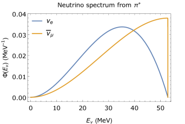
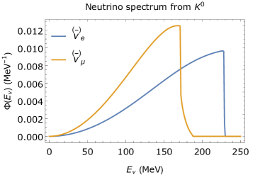
Figure 2: Neutrino spectrum from $\pi^{+}$ decay.

III.2 Background Flux

III.2.1 Solar Neutrino Flux

The solar neutrino flux around the Earth is estimated Haxton et al. (2013); Antonelli et al. (2013) to be about $\Phi_{\nu\odot}\sim 6.5\times 10^{11}\;\mathrm{cm}^{-2}\mathrm{s}^{-1}$. The energy range of such neutrinos is predicted by the Standard Solar Model (SSM) to be $E_{\nu\odot}\lesssim 10\;\mathrm{MeV}$, which is in a very different energy range to that under consideration. As such, the solar neutrino background is for our purposes negligible.

III.2.2 Atmospheric Neutrino Flux

The atmospheric neutrino flux can be modeled theoretically, such as in FLUKA Battistoni et al. (2005, 2003), Bartol Barr et al. (2004), and HKKM Honda et al. (2007, 2011, 2015). It is shown in Ref. Richard et al. (2016) that all three models are consistent with the Super-Kamiokande measurement. Therefore, we extract the value in Refs. Honda et al. (2015) to estimate the atmospheric neutrino background

$$\Phi_{\bar{\nu}_{e}+\nu_{e}} \approx 2.8\times 10^{-3}\left(\frac{R_{E}}{10\%}\right)\;\mathrm{cm}^{-2}\mathrm{s}^{-1}\mathrm{sr}^{-1}\,,$$ (40)

$$\Phi_{\bar{\nu}_{\mu}+\nu_{\mu}} \approx 6.2\times 10^{-3}\left(\frac{R_{E}}{10\%}\right)\;\mathrm{cm}^{-2}\mathrm{s}^{-1}\mathrm{sr}^{-1}\,,$$ (41)

where $R_{E}$ is the reconstructed energy resolution of the incident neutrino at the detector, which determines the bin width. For Super-Kamiokande Richard et al. (2016), the neutrino bin width is smaller at low energy (sub-GeV) and bigger at high energy (multi-GeV). For the angular resolution, the Sun’s angular span is about $6.8\times 10^{-5}\;\mathrm{sr}$, which is smaller than the angular resolution of most detectors, and so improved directional information could be useful for suppressing the atmospheric neutrino background even further.

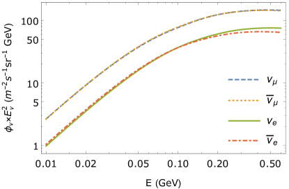
Figure 3: Atmosphere neutrino flux modeled in Honda et al. (2015). The blue (dashed), orange (dotted), green (solid), red (dash-dotted) correspond to $\nu_{\mu}$, $\bar{\nu}_{\mu}$, $\nu_{e}$, $\bar{\nu}_{e}$ respectively.

IV Detection Cross Section

In this section, we take into account the spectrum of the neutrino flux, and use Super-Kamiokande as a benchmark to calculate the cross section for a water Cherenkov detector. In a setup similar to Super-Kamiokande the target particles are electrons, protons, and oxygen nuclei. Neutrinos interact with them via both neutral current (NC) and charged current (CC) interactions. In Ref. Ueno et al. (2012), only interactions with electrons and protons are used for the low energy neutrinos, and so following their analysis we then suppose the charged current channel below $50\;\mathrm{MeV}$ is not clean enough and thus cannot be used for detection. In addition, we assume that these interactions can be excluded experimentally, and so do not provide an additional source of background either. We discuss the three interaction channels one by one.

IV.1 Interactions with Electrons

Even though this is the cleanest channel, as we will see next, the cross section is also the smallest of the three channels. The relevant interactions are elastic scattering (ES) processes, as the inverse muon decay channel has a threshold energy of $10.92\,\mathrm{GeV}\;$. In the Standard Model, the interaction between neutrino flavour $\alpha$ ($\alpha=e,\mu,\tau$) and the electron is described at low energies by the effective four fermion interaction

$$\mathcal{L}_{\mathrm{SM}}\;=\;-2\sqrt{2}\,G_{F}(\bar{\nu}_{\alpha}\gamma^{\mu}P_{L}\nu_{\alpha})\Bigl{[}\,g_{\alpha L}(\bar{e}\gamma_{\mu}P_{L}e)+g_{\alpha R}(\bar{e}\gamma_{\mu}P_{R}e)\,\Bigr{]}\,.$$ (42)

The coupling constants at tree level are given by $g_{\alpha R}=\sin^{2}\theta_{W}$ and $g_{\alpha L}=\sin^{2}\theta_{W}\pm\frac{1}{2}$, where the lower sign applies for $\alpha=\mu$ and $\tau$ (from $Z$ exchange only) and the upper sign applies for $\alpha=e$ (from both $Z$ and $W$ exchange). For antineutrinos, the values of $g_{\alpha L}$ and $g_{\alpha R}$ will be reversed. The differential cross section for neutrino-electron elastic scattering (ES) due to this interaction is given by

$$\frac{d{\sigma}_{\nu_{\alpha}}(E_{\nu_{\alpha}},T_{e})}{dT_{e}}=\frac{2G^{2}_{F}m_{e}}{\pi}\left[{g}^{2}_{\alpha L}+{g}^{2}_{\alpha R}\left(1-\dfrac{T_{e}}{E_{\nu_{\alpha}}}\right)^{2}-{g}_{\alpha L}{g}_{\alpha R}\dfrac{m_{e}T_{e}}{E_{\nu_{\alpha}}^{2}}\right]\,,$$ (43)

where, $m_{e}$ is the electron mass, $E_{\nu_{\alpha}}$ is the initial energy of neutrino flavour $\alpha$, and $T_{e}$ is the kinetic energy of the recoil electron, which has the range

$$0\;\leq\;T_{e}\;\leq\;T_{\max}(E_{\nu_{\alpha}})\;=\;\dfrac{E_{\nu_{\alpha}}}{1+m_{e}/2E_{\nu_{\alpha}}}\,.$$ (44)

IV.1.1 Low Energy Signal

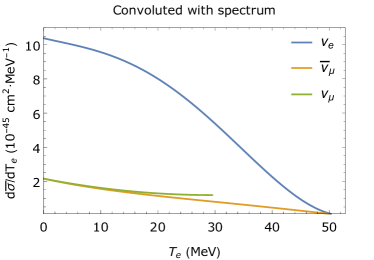
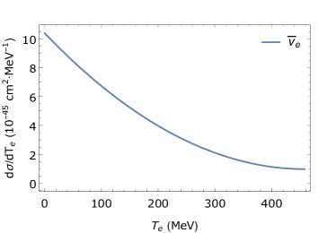
Figure 4: Left: convolution of neutrino spectrum from $\pi^{+}$ decay with differential cross section $d\sigma/dT_{e}$, where $T_{e}$ is the kinetic energy of the recoiling electrons. Right: the electron scattering cross section for $459\;\mathrm{MeV}$ antineutrinos.

We convolute the differential cross section $d\sigma/dT_{e}$ with the above spectrum, where $T_{e}$ is the electron’s recoil energy and

$$\frac{d\tilde{\sigma}}{dT_{e}} =\int_{E_{\nu},min}^{E_{\nu},max}\frac{d\sigma}{dT_{e}}(E_{\nu})\Phi(E_{\nu})dE_{\nu}\,,$$ (45)

as shown in Fig. 4. Following Ref. Ueno et al. (2012), an energy cut with respect to the recoiling electron ($T_{e}>20$ MeV) is performed to suppress the atmospheric neutrino background. The total cross section before and after the cut is

$$\sigma_{\nu_{e}}^{\mathrm{no\;cut}} =3.05\times 10^{-43}\;\mathrm{cm^{2}}\,,$$ (46)

$$\sigma_{\bar{\nu}_{\mu}}^{\mathrm{no\;cut}} =5.08\times 10^{-44}\;\mathrm{cm^{2}}\,,$$ (47)

$$\sigma_{\nu_{e}}^{\mathrm{no\;cut}} =4.48\times 10^{-44}\;\mathrm{cm^{2}}\,,$$ (48)

$$\sigma_{\nu_{e}} =1.16\times 10^{-43}\;\mathrm{cm^{2}}\,,$$ (49)

$$\sigma_{\bar{\nu}_{\mu}} =1.90\times 10^{-44}\;\mathrm{cm^{2}}\,,$$ (50)

$$\sigma_{\nu_{e}} =1.17\times 10^{-44}\;\mathrm{cm^{2}}\,.$$ (51)

Using the 5326 live days of Super-Kamiokande data Abe et al. (2017), we estimate the number of events for each flavour to be, after the energy cut

$$N_{\nu_{e}}\approx 4\,,\quad N_{\bar{\nu}_{\mu}}\approx 1\,,\quad N_{\nu_{\mu}}\approx 0\,.$$ (52)

IV.1.2 High Energy Signal

The differential cross section at high energy is shown in Fig. 4. The total cross section before and after the $20$ MeV cut is

$$\sigma_{\bar{\nu}_{e}}^{\mathrm{no\;cut}} =1.89\times 10^{-42}\;\mathrm{cm^{2}}\,,$$ (53)

$$\sigma_{\bar{\nu}_{e}} =1.69\times 10^{-42}\;\mathrm{cm^{2}}\,.$$ (54)

The number of events is

$$N_{\bar{\nu}e} \approx 5\,.$$ (55)

It is observed, due to the small cross section, that even when we saturate the Parker bound the number of events from electron interaction is very low. We will next calculate the signal and background from scattering events with protons and oxygen nuclei.

IV.2 Interactions with Protons

Neither the low energy neutrinos from pion decay or the 459 MeV neutrinos are energetic enough to cause Cherenkov radiation of the recoil protons. Therefore, the relevant channel is the inverse beta (muon) decay process, where

$$\bar{\nu}_{e}+p\rightarrow e^{+}+n\,,$$ (56)

$$\bar{\nu}_{\mu}+p\rightarrow\mu^{+}+n\,,$$ (57)

and the neutrons emit a 2.2 MeV $\gamma$ when they combine with protons later. This can be distinguished from the electron scattering events since neutron tagging became possible after the 2008 Super-Kamiokande IV upgrade Zhang et al. (2015). However, we do not base our analysis on this new neutron tagging technology.

The inverse muon decay process threshold is

$$E_{\bar{\nu}_{e},thres} =\frac{(E_{n}+E_{e})^{2}-m_{p}^{2}}{2m_{p}}=1.8\;\mathrm{MeV}\,,$$ (58)

$$E_{\bar{\nu}_{\mu},thres} =\frac{(E_{n}+E_{\mu})^{2}-m_{p}^{2}}{2m_{p}}=113.1\;\mathrm{MeV}\,.$$ (59)

Therefore, inverse muon decay is only relevant for the 459 MeV neutrinos and absent for low energy neutrinos. The cross section can be calculated numerically, or approximated analytically Strumia and Vissani (2003). We follow Ref. Strumia and Vissani (2003) and use the analytic expression for this analysis. The total cross section is reproduced and shown in Fig. 5.

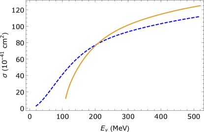
Figure 5: Total cross section of $\bar{\nu}_{e}+p\rightarrow e^{+}+n$ (blue dashed) and $\bar{\nu}_{\mu}+p\rightarrow\mu^{+}+n$ (orange solid), using the findings of Ref. Strumia and Vissani (2003).

IV.2.1 Low Energy Events

Integrating the formula in Ref. Strumia and Vissani (2003) with the neutrino spectrum in Fig. 4, we show the convoluted differential cross section in the left panel of Fig. 6.

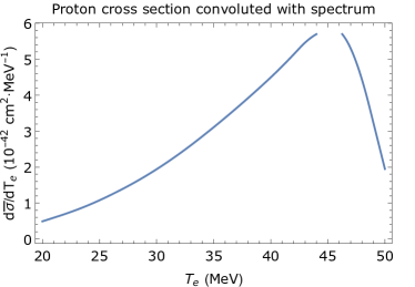
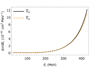
Figure 6: Left: convoluted cross section of low energy $\bar{\nu}_{e}p$ scattering. Right: Cross section of high energy antineutrino scattering from a proton target. The horizontal axis is the energy of the (electron or muon) recoil lepton.

After the energy cut, the total cross section is

$$\sigma_{\bar{\nu}_{e}} =9.21\times 10^{-41}\;\mathrm{cm}^{2}\,.$$ (60)

It is observed that from $\pi^{+}$ decay no $\bar{\nu}_{e}$ is directly produced. As $\bar{\nu}_{\mu}$ propagate to Earth, they oscillate to $\bar{\nu}_{e}$, as detailed in Section III.1. Using the 5326 live days of Super-Kamiokande data Abe et al. (2017), we estimate the number of events for $\bar{\nu}_{e}$ to be

$$N_{\bar{\nu}_{e}}\approx 194\,.$$ (61)

IV.2.2 High Energy Events

The differential cross section of 459 MeV antineutrino scattering is shown in the right panel of Fig. 6. Using the formula from Ref. Strumia and Vissani (2003), the total cross section is estimated to be

$$\sigma_{\bar{\nu}_{e}p}=1.08\times 10^{-39}\;\mathrm{cm^{2}}\,,\quad\sigma_{\bar{\nu}_{\mu}p}=1.20\times 10^{-39}\;\mathrm{cm^{2}}\,.$$ (62)

The number of events is

$$N_{\bar{\nu}_{e}}=235\,,\quad N_{\bar{\nu}_{\mu}}=324\,.$$ (63)

IV.2.3 Background Events

The neutrino/proton differential cross section convoluted with atmospheric neutrinos is shown in Fig. 7.

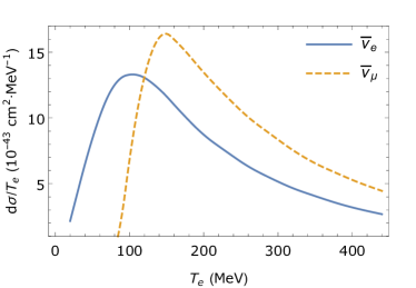
Figure 7: Differential cross section of antineutrino proton scattering, convoluted with background flux.

From 20 to 50 MeV, the number of background events is

$$N_{\bar{\nu}_{e}} =17\,.$$ (64)

At high energy, the number of background events is

$$N_{\bar{\nu}_{e}}=279\,,\quad N_{\bar{\nu}_{\mu}}=465\,.$$ (65)

We observe that the signal peaks at high energy, while the background peaks at below 200 MeV. Therefore, we can perform an energy cut to suppress the background. With for example a 300 MeV cut, the number of events for signal and background reads

$$N_{\bar{\nu}_{e}}^{signal}=220\,,\quad N_{\bar{\nu}_{\mu}}^{signal}=305\,,\quad N^{atm}_{\bar{\nu}_{e}}=49\,,\quad N^{atm}_{\bar{\nu}_{\mu}}=122\,,$$ (66)

from which we can see the background is suppressed by $\sim 80\%$, with less than $\sim 10\%$ signal cross section sacrificed. In the next section, we will show a more rigorous cut that optimises the statistical significance.

IV.3 Interactions with Oxygen

As noted in Ankowski et al. (2013, 2015), in the energy range of a few hundred MeV the single nucleon knock-out neutral current quasi-elastic (NCQE) scattering is significant. Predictions from various models are compared and shown in Fig. 1 there, where cross sections for antineutrinos knocking out a single neutron and a single proton are both around $3\times 10^{-39}\;\mathrm{cm}^{2}$. However, as there is no charged lepton emission, we do not use these processes for detection purposes.

Charged current quasi-elastic (CCQE) scattering takes place via the following processes

$$\bar{\nu}_{e}+{}^{16}\mathrm{O}\rightarrow e^{+}+{}^{16}\mathrm{N},$$ (67)

$$\bar{\nu}_{\mu}+{}^{16}\mathrm{O}\rightarrow\mu^{+}+{}^{16}\mathrm{N},$$ (68)

$$\nu_{e}+{}^{16}\mathrm{O}\rightarrow e^{-}+{}^{16}\mathrm{F},$$ (69)

$$\nu_{\mu}+{}^{16}\mathrm{O}\rightarrow\mu^{-}+{}^{16}\mathrm{F}.$$ (70)

We use the Monte Carlo software NuWro Golan et al. (2012) to calculate the $(\nu,{}^{16}O)$ cross section with $459\;\mathrm{MeV}$ $\bar{\nu}$ and the atmospheric neutrino flux, shown in Fig. 8. Again, the cross section of atmospheric neutrinos is the result of the convolution

$$\frac{d\tilde{\sigma}}{dT_{\ell}} =\int_{E_{\nu,min}}^{\infty}\frac{d\sigma}{dT_{\ell}}(E_{\nu},T_{\ell})\Phi(E_{\nu})\;dE_{\nu}\,,$$ (71)

where $E_{\nu,min}$ is the minimum energy required by the kinematics of the process, given a recoil lepton energy $T_{\ell}$. It is observed that the convoluted cross section of atmospheric neutrinos peaks at $\sim 200\;\mathrm{MeV}$. Similar to proton scattering, this can be understood as the result of two competing factors: when the neutrino energy increases, the neutrino-nucleus cross section increases, however the atmospheric neutrino flux also decreases, as shown in Fig. 3. This balance guarantees the separation of our signal and background.

IV.3.1 High Energy Events

The cross section and number of events for 459 MeV antineutrino scattering from oxygen are

$$\sigma_{\bar{\nu}_{e}{}^{16}O} =1.41\times 10^{-38}\;\mathrm{cm}^{2}\,,\qquad N_{\bar{\nu}_{e}{}^{16}O}\approx 1538\,,$$ (72)

$$\sigma_{\bar{\nu}_{\mu}{}^{16}O} =1.26\times 10^{-38}\;\mathrm{cm}^{2}\,,\qquad N_{\bar{\nu}_{\mu}{}^{16}O}\approx 1699\,.$$ (73)

IV.3.2 Background Events

The cross section above 100 MeV and corresponding number of 459 MeV neutrino scattering events with oxygen are

$$\sigma_{\bar{\nu}_{e}{}^{16}O} =2.94\times 10^{-39}\;\mathrm{cm}^{2}\qquad N_{\bar{\nu}_{e}{}^{16}O}\approx 885\,,$$ (74)

$$\sigma_{\nu_{e}{}^{16}O} =1.39\times 10^{-38}\;\mathrm{cm}^{2}\qquad N_{\nu_{e}{}^{16}O}\approx 4188\,,$$ (75)

$$\sigma_{\bar{\nu}_{\mu}{}^{16}O} =5.04\times 10^{-39}\;\mathrm{cm}^{2}\qquad N_{\bar{\nu}_{\mu}{}^{16}O}\approx 1518\,,$$ (76)

$$\sigma_{\nu_{\mu}{}^{16}O} =2.20\times 10^{-38}\;\mathrm{cm}^{2}\qquad N_{\nu_{\mu}{}^{16}O}\approx 6616\,.$$ (77)

Again, if we perform a 300 MeV energy cut, the signal and background are reduced to

$$N^{signal}_{\bar{\nu}_{e}{}^{16}O}\approx 1143\,,\qquad N^{atm}_{\bar{\nu}_{e}{}^{16}O} \approx 330\,,$$ (78)

$$N^{atm}_{\nu_{e}{}^{16}O} \approx 1457\,,$$ (79)

$$N^{signal}_{\bar{\nu}_{\mu}{}^{16}O}\approx 1351\,,\qquad N^{atm}_{\bar{\nu}_{\mu}{}^{16}O} \approx 638\,,$$ (80)

$$N^{atm}_{\nu_{\mu}{}^{16}O} \approx 2606\,.$$ (81)

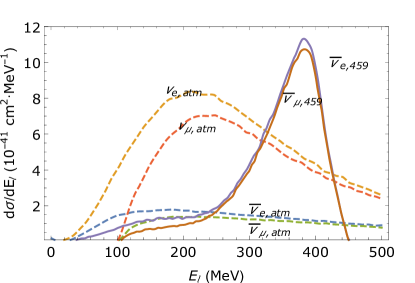
Figure 8: The differential cross section with ${}^{16}O$ of the $459\;\mathrm{MeV}$ monoenergetic antineutrino signal (solid) and the atmospheric neutrino background (dashed). It is observed that the recoiling electrons from atmospheric neutrinos peak at around 200 MeV, whilst those from our 459 MeV antineutrinos peak at around 400 MeV.

V Significance

In this section, we discuss the significance of both the high and low energy channels. In Ref.Ueno et al. (2012), low-energy solar neutrinos are used to bound the monopole flux $\phi_{M}$ to be

$$\phi_{M}\lesssim 6.3\times 10^{-8}\,,$$ (82)

at $90\%$ confidence level. Instead of going through a similar analysis with real data, we will compare the relative signal significance of the high and low energy channels for some fiducial values of $\phi_{M}$, to demonstrate that the 459 MeV antineutrinos ultimately offer better discovery potential. We construct the $\chi$-square via

$$\chi^{2} =\frac{(N_{exp}-N_{th})^{2}}{\sigma^{2}}=\frac{N^{2}_{\nu m}(\phi_{M})}{N_{atm}}\,,$$ (83)

where $N_{\nu m}$ is the number of neutrinos from monopole catalysed processes. We assume $N_{exp}=N_{atm}$, $N_{th}(\phi_{M})=N_{\nu m}(\phi_{M})+N_{atm}$, and that the statistical error dominates over systematic error. We only use the total number of events for the comparison and do not make use of the binning of the data in real experiments, as that shape information enhances the two channels equally. By letting $N_{\nu m}$ be the number of low or high energy neutrinos, we can find the signal significance of the two channels.

As is shown in previous sections, the cross sections of 459 MeV antineutrinos scattering off protons and oxygen nuclei peak at a lepton recoil energy different to that of the atmospheric neutrino background. To maximise the significance of the 459 MeV neutrino signal, we then float the energy cut position to maximise the $\chi^{2}$. In Fig. 9 we show the significance of the 459 MeV antineutrino signal, with a monopole flux that give a one $\sigma$ excess in the low energy neutrino channel. We observe the optimal cut position is at $E=364\;\mathrm{MeV}$.

Table 1: The signal (left) and background (right), with electron, proton, and oxygen target, for both channels. Please note that since Super-Kamiokande does not distinguish $\nu$ from $\bar{\nu}$, the background comprises both neutrinos and antineutrinos.

With this optimal energy cut, the number of events for both channels and the background are summarised in Table 1. We compare the statistical significance of the two channels and show the result in Fig. 9. It is observed that for example a $2\;\sigma$ deviation in the low energy channel will be amplified to $3\;\sigma$ in the 459 MeV channel, and a $3\;\sigma$ effect will be amplified to more than $4.6\;\sigma$. We also note that this is without combining the two channels and making use of their correlation, which is likely to enhance the result further.

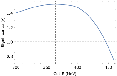
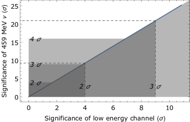
Figure 9: The statistical significance of 459 MeV antineutrino channel, with that of the low energy neutrino channel fixed at one standard deviation (left), and the comparison of the statistical significance of the two channels, given a fiducial monopole flux (right).

VI Discussion

As one of the most plausible aspects of physics beyond the Standard Model, magnetic monopoles have woven a persistent thread throughout particle physics for several decades. Whilst any hint of their discovery would be a sensation in that arena alone, it would also pose a very serious problem for inflationary theory, creating a very attractive experimental target. Thankfully their exotic properties also allow for a range of relatively unambiguous experimental signatures, aiding any discovery efforts.

To this end we have examined a previously untapped discovery channel, based on the monoenergetic 459 MeV antineutrinos produced via monopole-induced proton decay occurring inside the Sun. We do note that this process relies upon the survival of the GUT monopoles carrying electroweak magnetic charge to the present day, but under the plausible assumption of a straightforward screening mechanism for these electroweak effects, this is unproblematic. This channel was neglected in previous analyses due to the associated electroweak suppression factor, in favour of the unsuppressed 20 - 50 MeV neutrinos produced indirectly via monopole-induced proton decay to neutral mesons.

Due to the reduced experimental background and increased interaction cross section enjoyed by these high energy neutrinos, we have however demonstrated that they in fact can offer superior discovery potential. In particular, using 5326 live days of Super-Kamiokande exposure we found that $2\;\sigma$ ($3\;\sigma$) deviations in the 20-50 MeV channel correspond to $3\;\sigma$ ($4.6\;\sigma$) deviations in the 459 MeV case.

These effects could likely be further enhanced by leveraging the correlation between the two channels. Liquid scintillation neutrino detectors, such as the Deep Underground Neutrino Experiment (DUNE), may also offer some distinct advantages in detecting signals of this nature and thus even greater discovery potential Kumar and Sandick (2015); Rott et al. (2015, 2017).

Acknowledgments We would like to thank Lorenzo Calibbi, Shaomin Chen, Pilar Coloma, Tomasz Golan, Vishvas Pandey for useful communications. NH is supported by a CAS President’s International Fellowship. TL acknowledges the Projects 11475238, 11647601, and 11747601 supported by the National Natural Science Foundation of China, and by the Key Research Program of Frontier Science, CAS. CS is supported in part by the International Postdoctoral Fellowship funded by China Postdoctoral Science Foundation, and is grateful for the hospitality and partial support of the Department of Physics and Astronomy at Dartmouth College where this work was undertaken.

References

- Burdin et al. (2015) S. Burdin, M. Fairbairn, P. Mermod, D. Milstead, J. Pinfold, T. Sloan, and W. Taylor, Phys. Rept. 582, 1 (2015), eprint 1410.1374.
- Price et al. (1975) P. B. Price, E. K. Shirk, W. Z. Osborne, and L. S. Pinsky, Phys. Rev. Lett. 35, 487 (1975).
- Cabrera (1982) B. Cabrera, Phys. Rev. Lett. 48, 1378 (1982).
- Acharya et al. (2014) B. Acharya et al. (MoEDAL), Int. J. Mod. Phys. A29, 1430050 (2014), eprint 1405.7662.
- Ade et al. (2016) P. A. R. Ade et al. (Planck), Astron. Astrophys. 594, A20 (2016), eprint 1502.02114.
- Pinfold et al. (2009) J. Pinfold et al. (MoEDAL) (2009).
- Callan (1982) C. G. Callan, Jr., Phys. Rev. D26, 2058 (1982).
- Rubakov (1982) V. A. Rubakov, Nucl. Phys. B203, 311 (1982).
- Kolb et al. (1982) E. W. Kolb, S. A. Colgate, and J. A. Harvey, Phys. Rev. Lett. 49, 1373 (1982).
- Freese and Krasteva (1999) K. Freese and E. Krasteva, Phys. Rev. D59, 063007 (1999), eprint astro-ph/9804148.
- Arafune and Fukugita (1983) J. Arafune and M. Fukugita, Phys. Lett. 133B, 380 (1983).
- Ambrosio et al. (2002) M. Ambrosio et al. (MACRO), Eur. Phys. J. C25, 511 (2002), eprint hep-ex/0207020.
- Aartsen et al. (2014) M. G. Aartsen et al. (IceCube), Eur. Phys. J. C74, 2938 (2014), eprint 1402.3460.
- Aartsen et al. (2016) M. G. Aartsen et al. (IceCube), Eur. Phys. J. C76, 133 (2016), eprint 1511.01350.
- Ellis et al. (1982) J. R. Ellis, D. V. Nanopoulos, and K. A. Olive, Phys. Lett. 116B, 127 (1982).
- Bais et al. (1983) F. A. Bais, J. R. Ellis, D. V. Nanopoulos, and K. A. Olive, Nucl. Phys. B219, 189 (1983).
- Honda et al. (2015) M. Honda, M. Sajjad Athar, T. Kajita, K. Kasahara, and S. Midorikawa, Phys. Rev. D92, 023004 (2015), eprint 1502.03916.
- Ueno et al. (2012) K. Ueno et al. (Super-Kamiokande), Astropart. Phys. 36, 131 (2012), eprint 1203.0940.
- Polchinski (1984) J. Polchinski, Nucl. Phys. B242, 345 (1984).
- Montonen and Olive (1977) C. Montonen and D. I. Olive, Phys. Lett. 72B, 117 (1977).
- Chamseddine et al. (2013) A. H. Chamseddine, A. Connes, and W. D. van Suijlekom, JHEP 11, 132 (2013), eprint 1304.8050.
- Aydemir et al. (2016) U. Aydemir, D. Minic, C. Sun, and T. Takeuchi, Int. J. Mod. Phys. A31, 1550223 (2016), eprint 1509.01606.
- Dawson and Schellekens (1983) S. Dawson and A. N. Schellekens, Phys. Rev. D27, 2119 (1983).
- Liu and Vachaspati (1997) H. Liu and T. Vachaspati, Phys. Rev. D56, 1300 (1997), eprint hep-th/9604138.
- Dokos and Tomaras (1980) C. P. Dokos and T. N. Tomaras, Phys. Rev. D21, 2940 (1980).
- Lazarides and Shafi (1980) G. Lazarides and Q. Shafi, Phys. Lett. 94B, 149 (1980).
- Sakai and Yanagida (1982) N. Sakai and T. Yanagida, Nucl. Phys. B197, 533 (1982).
- Gardner and Harvey (1984) C. L. Gardner and J. A. Harvey, Phys. Rev. Lett. 52, 879 (1984).
- Vachaspati (1996) T. Vachaspati, Phys. Rev. Lett. 76, 188 (1996), eprint hep-ph/9509271.
- Parker (1970) E. N. Parker, Astrophys. J. 160, 383 (1970).
- Kuzmin and Rubakov (1983) V. A. Kuzmin and V. A. Rubakov, Phys. Lett. 125B, 372 (1983).
- Frieman et al. (1988) J. A. Frieman, K. Freese, and M. S. Turner, Astrophys. J. 335, 844 (1988).
- Hill (1983) C. T. Hill, Nucl. Phys. B224, 469 (1983).
- Agarwalla et al. (2014) S. K. Agarwalla, Y. Kao, and T. Takeuchi, JHEP 04, 047 (2014), eprint 1302.6773.
- Haxton et al. (2013) W. C. Haxton, R. G. Hamish Robertson, and A. M. Serenelli, Ann. Rev. Astron. Astrophys. 51, 21 (2013), eprint 1208.5723.
- Antonelli et al. (2013) V. Antonelli, L. Miramonti, C. Pena Garay, and A. Serenelli, Adv. High Energy Phys. 2013, 351926 (2013), eprint 1208.1356.
- Battistoni et al. (2005) G. Battistoni, A. Ferrari, T. Montaruli, and P. Sala, Astroparticle Physics 23, 526 (2005).
- Battistoni et al. (2003) G. Battistoni, A. Ferrari, T. Montaruli, and P. R. Sala, Astropart. Phys. 19, 269 (2003), [Erratum: Astropart. Phys.19,291(2003)], eprint hep-ph/0207035.
- Barr et al. (2004) G. D. Barr, T. K. Gaisser, P. Lipari, S. Robbins, and T. Stanev, Phys. Rev. D70, 023006 (2004), eprint astro-ph/0403630.
- Honda et al. (2007) M. Honda, T. Kajita, K. Kasahara, S. Midorikawa, and T. Sanuki, Phys. Rev. D75, 043006 (2007), eprint astro-ph/0611418.
- Honda et al. (2011) M. Honda, T. Kajita, K. Kasahara, and S. Midorikawa, Phys. Rev. D83, 123001 (2011), eprint 1102.2688.
- Richard et al. (2016) E. Richard et al. (Super-Kamiokande), Phys. Rev. D94, 052001 (2016), eprint 1510.08127.
- Abe et al. (2017) K. Abe et al. (Super-Kamiokande) (2017), eprint 1710.09126.
- Zhang et al. (2015) H. Zhang et al. (Super-Kamiokande), Astropart. Phys. 60, 41 (2015), eprint 1311.3738.
- Strumia and Vissani (2003) A. Strumia and F. Vissani, Phys. Lett. B564, 42 (2003), eprint astro-ph/0302055.
- Ankowski et al. (2013) A. M. Ankowski, O. Benhar, T. Mori, R. Yamaguchi, and M. Sakuda, J. Phys. Conf. Ser. 408, 012055 (2013), eprint 1202.0227.
- Ankowski et al. (2015) A. M. Ankowski, M. B. Barbaro, O. Benhar, J. A. Caballero, C. Giusti, R. González-Jiménez, G. D. Megias, and A. Meucci, Phys. Rev. C92, 025501 (2015), eprint 1506.02673.
- Golan et al. (2012) T. Golan, C. Juszczak, and J. T. Sobczyk, Phys. Rev. C86, 015505 (2012), eprint 1202.4197.
- Kumar and Sandick (2015) J. Kumar and P. Sandick, JCAP 1506, 035 (2015), eprint 1502.02091.
- Rott et al. (2015) C. Rott, S. In, J. Kumar, and D. Yaylali, JCAP 1511, 039 (2015), eprint 1510.00170.
- Rott et al. (2017) C. Rott, S. In, J. Kumar, and D. Yaylali, JCAP 1701, 016 (2017), eprint 1609.04876.