Fundamental limits to quantum channel discrimination

Abstract

What is the ultimate performance for discriminating two arbitrary quantum channels acting on a finite-dimensional Hilbert space? Here we address this basic question by deriving a general and fundamental lower bound. More precisely, we investigate the symmetric discrimination of two arbitrary qudit channels by means of the most general protocols based on adaptive (feedback-assisted) quantum operations. In this general scenario, we first show how port-based teleportation can be used to simplify these adaptive protocols into a much simpler non-adaptive form, designing a new type of teleportation stretching. Then, we prove that the minimum error probability affecting the channel discrimination cannot beat a bound determined by the Choi matrices of the channels, establishing a general, yet computable formula for quantum hypothesis testing. As a consequence of this bound, we derive ultimate limits and no-go theorems for adaptive quantum illumination and single-photon quantum optical resolution. Finally, we show how the methodology can also be applied to other tasks, such as quantum metrology, quantum communication and secret key generation.

I Introduction

Quantum hypothesis testing QHT1 is a central area in quantum information theory Watrous ; HolevoBOOK , with many studies for both discrete variable (DV) NiCh and continuous variable (CV) systems RMP . A number of tools QCB1 ; QCB2 ; QCB3 ; QHB1 ; QHB2 have been developed for its basic formulation, known as quantum state discrimination. In particular, since the seminal work of Helstrom in the 70s QHT1 , we know how to bound the error probability affecting the symmetric discrimination of two arbitrary quantum states. Remarkably, after about 40 years, a similar bound is still missing for the discrimination of two arbitrary quantum channels. There is a precise motivation for that: The main problem in quantum channel discrimination (QCD) QCD1 ; QCD2 ; QCD3 ; QCD4 ; QCD6 is that the strategies involve an optimization over the input states and the output measurements, and this process may be adaptive in the most general case, so that feedback from the output can be used to update the input.

Not only the ultimate performance of adaptive QCD is still unknown due to the difficulty of handling feedback-assistance, but it is also known that adaptiveness needs to be considered in QCD. In fact, apart from the cases where two channels are classical HayaCLASS , jointly programmable or teleportation-covariant PirCo ; ReviewMETRO , feedback may greatly improve the discrimination. For instance, Ref. Harrow  presented two channels which can be perfectly distinguished by using feedback in just two adaptive uses, while they cannot be perfectly discriminated by any number of uses of a block (non-adaptive) protocol, where the channels are probed in an identical and independent fashion. This suggests that the best discrimination performance is not directly related to the diamond distance Diamond , when computed over multiple copies of the quantum channels.

In this work we finally fill this fundamental gap by deriving a universal computable lower bound for the error probability affecting the discrimination of two arbitrary quantum channels. To derive this bound we adopt a technique which reduces an adaptive protocol over an arbitrary finite-dimensional quantum channel into a block protocol over multiple copies of the channel’s Choi matrix. This is obtained by using port-based teleportation (PBT) PBT ; PBT1 ; PBT2 ; Brau for channel simulation and suitably generalizing the technique of teleportation stretching PLOB ; TQC ; Uniform . This reduction is shown for adaptive protocols with any task (not just QCD). When applied to QCD, it allows us to bound the ultimate error probability by using the Choi matrices of the channels.

As a direct application, we bound the ultimate adaptive performance of quantum illumination Qill0 ; Qill1 ; Qill2 ; Qill3 ; Qill4 ; Qill6 ; Qill7 ; Qill8 and the ultimate adaptive resolution of any single-photon diffraction-limited optical system, setting corresponding no-go theorems for these applications. We then apply our result to adaptive quantum metrology showing an ultimate bound which has an asymptotic Heisenberg scaling. As an example, we also study the adaptive discrimination of amplitude damping channels, which are the most difficult channels to be simulated. Finally, other implications are for the two-way assisted capacities of quantum and private communications.

II Results

II.1 Adaptive protocols

Let us formulate the most general adaptive protocol over an arbitrary quantum channel $\mathcal{E}$ defined between Hilbert spaces of dimension $d$ (more generally, this can be taken as the dimension of the input space). We first provide a general description and then we specify the protocol to the task of QCD. A general adaptive protocol involves an unconstrained number of quantum systems which may be subject to completely arbitrary quantum operations (QOs). More precisely, we may organize the quantum systems into an input register $\mathbf{a}$ and an output register $\mathbf{b}$, which are prepared in an initial state $\rho_{0}$ by applying a QO $\Lambda_{0}$ to some fundamental state of $\mathbf{a}$ and $\mathbf{b}$. Then, a system $a_{1}$ is picked from the register $\mathbf{a}$ and sent through the channel $\mathcal{E}$. The corresponding output $b_{1}$ is merged with the output register $b_{1}\mathbf{b\rightarrow b}$. This is followed by another QO $\Lambda_{1}$ applied to $\mathbf{a}$ and $\mathbf{b}$. Then, we send a second system $a_{2}\in\mathbf{a}$ through $\mathcal{E}$ with the output $b_{2}$ being merged again $b_{2}\mathbf{b\rightarrow b}$ and so on. After $n$ uses, the registers will be in a state $\rho_{n}$ which depends on $\mathcal{E}$ and the sequence of QOs $\{\Lambda_{0},\Lambda_{1},\ldots,\Lambda_{n}\}$ defining the adaptive protocol $\mathcal{P}_{n}$ with output state $\rho_{n}$ (see Fig. 1).

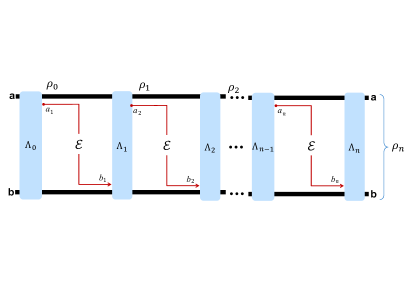
Figure 1: General structure of an adaptive quantum protocol, where channel uses $\mathcal{E}$ are interleaved by QOs $\Lambda$’s. See text for more details.

In a protocol of quantum communication, the registers belong to remote users and, in absence of entanglement-assistance, the QOs are local operations (LOs) assisted by two-way classical communication (CC), also known as adaptive LOCCs. The output is generated in such a way to approximate some target state PLOB . In a protocol of quantum channel estimation, the channel is labelled by a continuous parameter $\mathcal{E}=\mathcal{E}_{\theta}$ and the QOs include the use of entanglement across the registers. The output state will encode the unknown parameter $\rho_{n}=\rho_{n}(\theta)$, which is detected and the outcome processed into an optimal estimator PirCo . Here, in a protocol of binary and symmetric QCD, the channel is labelled by a binary digit, i.e., $\mathcal{E}=\mathcal{E}_{u}$ where $u\in\{0,1\}$ has equal priors. The QOs are generally entangled and they generate an output state encoding the information bit, i.e., $\rho_{n}=\rho_{n}(u)$.

The output state $\rho_{n}(u)$ of an adaptive discrimination protocol $\mathcal{P}_{n}$ is finally detected by an optimal positive-operator valued measure (POVM). For binary discrimination, this is the Helstrom POVM, which leads to the conditional error probability

$$p(\mathcal{E}_{0}\neq\mathcal{E}_{1}|\mathcal{P}_{n})=\frac{1-D\left[\rho_{n}(0),\rho_{n}(1)\right]}{2},$$ (1)

where $D(\rho,\sigma):=||\rho-\sigma||/2$ is the trace distance NiCh . The optimization over all discrimination protocols $\mathcal{P}_{n}$ defines the minimum error probability affecting the $n$-use adaptive discrimination of $\mathcal{E}_{0}$ and $\mathcal{E}_{1}$, i.e., we may write

$$p_{n}(\mathcal{E}_{0}\neq\mathcal{E}_{1}):=\inf_{\mathcal{P}_{n}}~{}p(\mathcal{E}_{0}\neq\mathcal{E}_{1}|\mathcal{P}_{n}).$$ (2)

This is generally less than the $n$-copy diamond distance between the two channels $\mathcal{E}_{0}^{\otimes n}$ and $\mathcal{E}_{1}^{\otimes n}$

$$p_{n}(\mathcal{E}_{0}\neq\mathcal{E}_{1})\leq\frac{1-\frac{1}{2}||\mathcal{E}_{0}^{\otimes n}-\mathcal{E}_{1}^{\otimes n}||_{\diamond}}{2},$$ (3)

where Watrous

$$||\mathcal{E}_{0}^{\otimes n}-\mathcal{E}_{1}^{\otimes n}||_{\diamond}:=\sup_{\rho_{ar}}||\mathcal{E}_{0}^{\otimes n}\otimes\mathcal{I}(\rho_{ar})-\mathcal{E}_{1}^{\otimes n}\otimes\mathcal{I}(\rho_{ar})||,$$ (4)

with $\mathcal{I}$ being an identity map acting on a reference system $r$. The upper bound in Eq. (3) is achieved by a non-adaptive protocol, where an (optimal) input state $\rho_{ar}$ is prepared and its $a$-parts transmitted through $\mathcal{E}_{u}^{\otimes n}$. Note that Eq. (3) is very difficult to compute, which is why we usually compute larger but simpler single-letter upper bounds such as

$$p_{n}(\mathcal{E}_{0}\neq\mathcal{E}_{1})\leq\frac{F(\rho_{\mathcal{E}_{0}},\rho_{\mathcal{E}_{1}})^{n}}{2},$$ (5)

where $F$ is the fidelity between the Choi matrices, $\rho_{\mathcal{E}_{0}}$ and $\rho_{\mathcal{E}_{1}}$, of the two channels.

Our question is: Can we complete Eq. (3) with a corresponding lower bound? Up to today this has been only proven for jointly-programmable channels, i.e., channels $\mathcal{E}_{0}$ and $\mathcal{E}_{1}$ admitting a simulation $\mathcal{E}_{u}(\rho)=\mathcal{S}(\rho\otimes\pi_{u})$ with a trace-preserving QO $\mathcal{S}$ and different program states $\pi_{0}$ and $\pi_{1}$. In this case, we have $p_{n}\geq[1-D(\pi_{0}^{\otimes n},\pi_{1}^{\otimes n})]/2$ PirCo . In particular, this is true if the channels are jointly teleportation-covariant, so that $\mathcal{S}$ becomes teleportation and the program state is a Choi matrix $\rho_{\mathcal{E}_{u}}$. For these channels, Ref. PirCo found that Eq. (3) holds with an equality and we may write $||\mathcal{E}_{0}^{\otimes n}-\mathcal{E}_{1}^{\otimes n}||_{\diamond}=||\rho_{\mathcal{E}_{0}}^{\otimes n}-\rho_{\mathcal{E}_{1}}^{\otimes n}||$. More precisely, the question to ask is therefore the following: Can we establish a universal lower bound for $p_{n}(\mathcal{E}_{0}\neq\mathcal{E}_{1})$ which is valid for arbitrary channels? As we show here, this is possible by resorting to a more general (multi-program) simulation of the channels, i.e., of the type $\mathcal{S}(\rho\otimes\pi_{u}^{\otimes M})$.

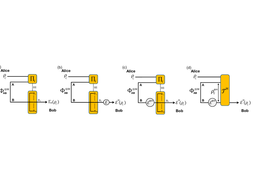
Figure 2: From port-based teleportation (PBT) to Choi-simulation of a quantum channel (see also Ref. PBT ). (a) Schematic representation of the PBT protocol. Alice and Bob share an $M\times M$ qudit state which is given by $M$ maximally-entangled states $\Phi_{\mathbf{AB}}^{\otimes M}$. To teleport an input qubit state $\rho_{C}$, Alice applies a suitable POVM $\{\Pi_{i}\}$ to the input qubit $C$ and her $\mathbf{A}$ qubits. The outcome $i$ is communicated to Bob, who selects the $i$-th among his $\mathbf{B}$ qubits (tracing all the others). The performance does not depend on the specific “port” $i$ selected and the average output state is given by $\Gamma_{M}(\rho_{C})$ where $\Gamma_{M}$ is the PBT channel. The latter reduces to the identity channel in the limit of many ports $M\rightarrow\infty$. (b) Suppose that Bob applies a quantum channel $\mathcal{E}$ on his teleported output. This produces the output state $\mathcal{E}^{M}(\rho_{C})$ of Eq. (12). For large $M$, one has $\mathcal{E}^{M}\rightarrow\mathcal{E}$ in diamond norm. (c) Equivalently, Bob can apply $\mathcal{E}^{\otimes M}$ to all his qubits $\mathbf{B}$ in advance to the CC from Alice. After selection of the port, this will result in the same output as before. (d) Now note that Alice’s LO and Bob’s port selection form a global LOCC $\mathcal{T}^{M}$ (trace-preserving by averaging over the outcomes). This is applied to a tensor-product state $\rho_{\mathcal{E}}^{\otimes M}$ where $\rho_{\mathcal{E}}$ is the Choi matrix of the original channel $\mathcal{E}$. Thus the approximate channel $\mathcal{E}^{M}$ is simulated by applying $\mathcal{T}^{M}$ to $\rho_{C}\otimes\rho_{\mathcal{E}}^{\otimes M}$ as in Eq. (13).

II.2 PBT and simulation of the identity

Let us describe the protocol of PBT with qudits of arbitrary dimension $d\geq 2$. More technical details can be found in the original proposals PBT1 ; PBT2 . The parties exploit two ensembles of $M\geq 2$ qudits, i.e., Alice has $\mathbf{A}:=\{A_{1},\ldots,A_{M}\}$ and Bob has $\mathbf{B}:=\{B_{1},\ldots,B_{M}\}$ representing the output “ports”. The generic $i$th pair $(A_{i},B_{i})$ is prepared in a maximally-entangled state, so that we have the global state

$$\Phi_{\mathbf{AB}}^{\otimes M}=\bigotimes_{i=1}^{M}|\Phi\rangle_{i}\langle\Phi|,~{}~{}|\Phi\rangle_{i}:=d^{-1/2}\sum_{k}\left|k\right\rangle_{A_{i}}\otimes\left|k\right\rangle_{B_{i}}.$$ (6)

To teleport the state of a qudit $C$, Alice performs a joint measurement on $C$ and her ensemble $\mathbf{A}$. This is a POVM $\{\Pi_{C\mathbf{A}}^{i}\}_{i=1}^{M}$ with $M$ possible outcomes (see Refs. PBT1 ; PBT2 for the details). In the standard protocol considered here, this POVM is a square root measurement (known to be optimal in the qubit case). Once Alice communicates the outcome $i$ to Bob, he discards all the ports but the $i$th one, which contains the teleported state (see Fig. 2a).

The measurement outcomes are equiprobable and independent of the input, and the output state is invariant under permutation of the ports (this can be understood by the fact that the scheme is invariant under permutation of the Bell states and, therefore, of the ports). Averaging over the outcomes, we define the teleported state $\rho_{B}^{M}=\Gamma_{M}(\rho_{C})$, where $\Gamma_{M}$ is the corresponding PBT channel. Explicitly, this channel takes the form

$$\Gamma_{M}(\rho_{C})=\sum_{i=1}^{M}\mathrm{Tr}_{\mathbf{A}\bar{B_{i}}C}[\Pi_{C\mathbf{A}}^{i}\left(\rho_{C}\otimes\Phi_{\mathbf{AB}}^{\otimes M}\right)],$$ (7)

where $\text{Tr}_{\bar{B_{i}}}$ denotes the trace over all ports $\mathbf{B}$ but $B_{i}$.

As shown in Ref. PBT1 , the standard protocol gives a depolarizing channel NiCh whose probability $\xi_{M}$ decreases to zero for increasing number of ports $M$. Therefore, in the limit of many ports $M\gg 1$, the $M$-port PBT channel $\Gamma_{M}$ tends to an identity channel $\mathcal{I}$, so that Bob’s output becomes a perfect replica of Alice’s input. Here we prove a stronger result in terms of channel uniform convergence TQC ; Uniform . In fact, for any $M$, we show that the simulation error, expressed in terms of the diamond distance between $\Gamma_{M}$ and $\mathcal{I}$, is one-to-one with the entanglement fidelity of the PBT channel $\Gamma_{M}$. In turn, this result allows us to write a simple upper bound for this error. Moreover, we can fully characterize the simulation error with an exact analytical expression for qubits (see Methods for the proof, with further details being given in Supplementary Section I).

Lemma 1

In arbitrary (finite) dimension $d$, the diamond distance between the $M$-port PBT channel $\Gamma_{M}$ and the identity channel $\mathcal{I}$ satisfies

$$\delta_{M}:=||\mathcal{I}-\Gamma_{M}||_{\diamond}=2[1-f_{e}(\Gamma_{M})],$$ (8)

where $f_{e}(\Gamma_{M}):=\langle\Phi|[\mathcal{I}\otimes\Gamma_{M}(|\Phi\rangle\langle\Phi|)]|\Phi\rangle$ is the entanglement fidelity of $\Gamma_{M}$. This gives the upper bound

$$\delta_{M}\leq 2d(d-1)M^{-1}~{}.$$ (9)

More precisely, we can write the exact result

$$\delta_{M}=\frac{2\left(d^{2}-1\right)}{d^{2}}\xi_{M},$$ (10)

where $\xi_{M}$ is the depolarizing probability of the PBT channel $\Gamma_{M}$. For qubits ($d=2$), the “PBT number” $\xi_{M}$ has the closed analytical expression

$$\xi_{M} =\frac{1}{3}\frac{M+2}{2^{M-1}}+\frac{1}{3}\sum_{s=s_{min}}^{(M-1)/2}\frac{s(s+1)}{2^{M-4}}\binom{M}{\frac{M-1}{2}-s}\times$$

$$\frac{\left(M+2\right)-\sqrt{\left(M+2\right)^{2}-\left(2s+1\right)^{2}}}{\left(M+2\right)^{2}-\left(2s+1\right)^{2}},$$ (11)

where $s_{min}=1/2$ for even $M$ and $0$ for odd $M$.

II.3 General channel simulation via PBT

Let us discuss how PBT can be used for channel simulation. This was first shown in Ref. PBT  where PBT was introduced as a possible design for a programmable quantum gate array Array . As depicted in Fig. 2b, suppose that Bob applies an arbitrary channel $\mathcal{E}$ to the teleported output, so that Alice’s input $\rho_{C}$ is subject to the approximate channel

$$\mathcal{E}^{M}(\rho_{C}):=\mathcal{E}\circ\Gamma_{M}(\rho_{C}).$$ (12)

Note that the port selection commutes with $\mathcal{E}$, because the POVM acts on a different Hilbert space PBT . Therefore, Bob can equivalently apply $\mathcal{E}$ to each port before Alice’s CC, i.e., apply $\mathcal{E}^{\otimes M}$ to his $\mathbf{B}$ qudits before selecting the output port, as shown in Fig. 2c. This leads to the following simulation for the approximate channel

$$\mathcal{E}^{M}(\rho_{C})=\mathcal{T}^{M}(\rho_{C}\otimes\rho_{\mathcal{E}}^{\otimes M})~{},$$ (13)

where $\mathcal{T}^{M}$ is a trace-preserving LOCC and $\rho_{\mathcal{E}}$ is the channel’s Choi matrix (see Fig. 2d). By construction, the simulation LOCC $\mathcal{T}^{M}$ is universal, i.e., it does not depend on the channel $\mathcal{E}$. This means that, at fixed $M$, the channel $\mathcal{E}^{M}$ is fully determined by the program state $\rho_{\mathcal{E}}$. One can bound the accuracy of the simulation. From Eq. (12) and the monotonicity of the diamond norm, we get

$$||\mathcal{E}-\mathcal{E}^{M}||_{\diamond}\leq\delta_{M},$$ (14)

where $\delta_{M}$ is the simulation error in Eq. (9), with the dimension $d$ being the one of the input Hilbert space. It is worth to remark that, while the simulation in Eq. (13) relies on a number of copies of the channel’s Choi matrix, it can be applied to an arbitrary quantum channel $\mathcal{E}$ without the condition of teleportation covariance PLOB .

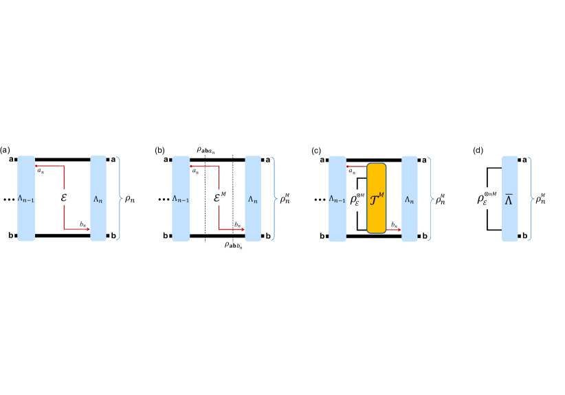
Figure 3: Port-based teleportation stretching of a generic adaptive protocol over a quantum channel $\mathcal{E}$. This channel is fixed in quantum/private communication, while it is unknown and parametrized in estimation/discrimination problems. (a) We show the last transmission $a_{n}\rightarrow b_{n}$ through $\mathcal{E}$, which occurs between two adaptive QOs $\Lambda_{n-1}$ and $\Lambda_{n}$. This last step produces the output state $\rho_{n}$. (b) In each transmission, we replace $\mathcal{E}$ with its $M$-port simulation $\mathcal{E}^{M}$ so that the output of the protocol becomes $\rho_{n}^{M}$ which approximates $\rho_{n}$ for large $M$. Note that, in the last transmission, the register state $\rho_{\mathbf{ab}a_{n}}$ undergoes the transformation $\rho_{\mathbf{ab}b_{n}}=\mathcal{I}_{\mathbf{ab}}\otimes\mathcal{E}^{M}(\rho_{\mathbf{ab}a_{n}})$. (c) Each propagation through $\mathcal{E}^{M}$ is replaced by its PBT simulation. For the last transmission, this means that $\rho_{\mathbf{ab}b_{n}}=\mathcal{I}_{\mathbf{ab}}\otimes\mathcal{T}^{M}(\rho_{\mathbf{ab}a_{n}}\otimes\rho_{\mathcal{E}}^{\otimes M})$ where $\mathcal{T}^{M}$ is the LOCC of the PBT and $\rho_{\mathcal{E}}$ is the Choi matrix of the original channel. (d) All the adaptive QOs $\Lambda_{i}$ and the simulation LOCCs $\mathcal{T}^{M}$ are collapsed into a single (trace-preserving) QO $\bar{\Lambda}$. Correspondingly, $n$ instances of $\rho_{\mathcal{E}}^{\otimes M}$ are collected. As a result, the approximate output $\rho_{n}^{M}$ is given by $\bar{\Lambda}$ applied to the tensor-product state $\rho_{\mathcal{E}}^{\otimes nM}$ as in Eq. (16).

II.4 PBT stretching of an adaptive protocol

Channel simulation is a preliminary tool for the following technique of teleportation stretching, where an arbitrary adaptive protocol is reduced into a simpler block version. There are two main steps. First of all, we need to replace each channel $\mathcal{E}$ with its $M$-port approximation $\mathcal{E}^{M}$ while controlling the propagation of the simulation error $\delta_{M}$ from the channel to the output state. This step is crucial also in simulations via standard teleportation TQC ; ReviewMETRO (see also Refs. networkPIRS ; Multipoint ; finiteStretching ; nonPauli ; HWchannels ). Second, we need to “stretch” the protocol PLOB by replacing the various instances of the approximate channel $\mathcal{E}^{M}$ with a collection of Choi matrices $\rho_{\mathcal{E}}^{\otimes M}$ and then suitably re-organizing all the remaining QOs. Here we describe the technique for a generic task, before specifying it to QCD.

Given an adaptive protocol $\mathcal{P}_{n}$ over a channel $\mathcal{E}$ with output $\rho_{n}$, consider the same protocol over the simulated channel $\mathcal{E}^{M}$, so that we get the different output $\rho_{n}^{M}$. Using a “peeling” argument (see Methods), we bound the output error in terms of the channel simulation error

$$||\rho_{n}-\rho_{n}^{M}||\leq n||\mathcal{E}-\mathcal{E}^{M}||_{\diamond}\leq n\delta_{M}.$$ (15)

Once understood that the output state can be closely approximated, let us simplify the adaptive protocol over $\mathcal{E}^{M}$. Using the simulation in Eq. (13), we may replace each channel $\mathcal{E}^{M}$ with the resource state $\rho_{\mathcal{E}}^{\otimes M}$, iterate the process for all $n$ uses, and collapse all the simulation LOCCs and QOs as shown in Fig. 3. As a result, we may write the multi-copy Choi decomposition

$$\rho_{n}^{M}=\bar{\Lambda}(\rho_{\mathcal{E}}^{\otimes nM})~{},$$ (16)

for a trace-preserving QO $\bar{\Lambda}$. Now, we can combine the two ingredients of Eqs. (15) and (16), into the following.

Lemma 2 (PBT stretching)

Consider an adaptive quantum protocol (with arbitrary task) over an arbitrary $d$-dimensional quantum channel $\mathcal{E}$ (which may be unknown and parametrized). After $n$ uses, the output $\rho_{n}$ of the protocol can be decomposed as follows

$$||\rho_{n}-\bar{\Lambda}(\rho_{\mathcal{E}}^{\otimes nM})||\leq n\delta_{M},$$ (17)

where $\bar{\Lambda}$ is a trace-preserving QO, $\rho_{\mathcal{E}}$ is the Choi matrix of $\mathcal{E}$, and $\delta_{M}$ is the $M$-port simulation error in Eq. (9).

When we apply the lemma to protocols of quantum or private communication, where the QOs $\Lambda_{i}$ are LOCCs, then we may write Eq. (17) with $\bar{\Lambda}$ being a LOCC. In protocols of channel estimation or discrimination, where $\mathcal{E}$ is parametrized, we may write Eq. (17) with $\rho_{\mathcal{E}}$ storing the parameter of the channel. In particular, for QCD we have $\{\mathcal{E}_{u}\}_{u=0,1}$ and the output $\rho_{n}(u)$ of the adaptive protocol $\mathcal{P}_{n}$ can be decomposed as follows

$$||\rho_{n}(u)-\bar{\Lambda}(\rho_{\mathcal{E}_{u}}^{\otimes nM})||\leq n\delta_{M}.$$ (18)

II.5 Ultimate bound for channel discrimination

We are now ready to show the lower bound for minimum error probability $p_{n}(\mathcal{E}_{0}\neq\mathcal{E}_{1})$ in Eq. (3). Consider an arbitrary protocol $\mathcal{P}_{n}$, for which we may write Eq. (1). Combining Lemma 2 with the triangle inequality leads to

$$||\rho_{n}(0)-\rho_{n}(1)|| \leq 2n\delta_{M}+||\bar{\Lambda}(\rho_{\mathcal{E}_{0}}^{\otimes nM})-\bar{\Lambda}(\rho_{\mathcal{E}_{1}}^{\otimes nM})||$$

$$\leq 2n\delta_{M}+||\rho_{\mathcal{E}_{0}}^{\otimes nM}-\rho_{\mathcal{E}_{1}}^{\otimes nM}||,$$ (19)

where we also use the monotonicity of the trace distance under channels. Because $\bar{\Lambda}$ is lost, the bound does no longer depend on the details of the protocol $\mathcal{P}_{n}$, which means that it applies to all adaptive protocols. Thus, using Eq. (19) in Eqs. (1) and (2), we get the following.

Theorem 3

Consider the adaptive discrimination of two channels $\{\mathcal{E}_{u}\}_{u=0,1}$ in dimension $d$. After $n$ probings, the minimum error probability satisfies the bound

$$p_{n}(\mathcal{E}_{0}\neq\mathcal{E}_{1})\geq B:=\frac{1-n\delta_{M}-D(\rho_{\mathcal{E}_{0}}^{\otimes nM},\rho_{\mathcal{E}_{1}}^{\otimes nM})}{2},$$ (20)

where $M$ may be chosen to maximize the right hand side.

Not only this is the first universal bound for adaptive QCD, but also its analytical form is rather surprising. In fact, its tighest value is given by an optimal (finite) number of ports $M$ for the underlying protocol of PBT.

Let us bound the trace distance in Eq. (20) as

$$D^{2}\leq 1-F^{2nM},~{}F:=\mathrm{Tr}\sqrt{\sqrt{\rho_{\mathcal{E}_{0}}}\rho_{\mathcal{E}_{1}}\sqrt{\rho_{\mathcal{E}_{0}}}},$$ (21)

where $F$ is the fidelity between the Choi matrices of the channels. This comes from the Fuchs-van de Graaf relations Fuchs and the multiplicativity of the fidelity over tensor products. Other bounds that can be written are

$$D\leq nM\left\|\rho_{\mathcal{E}_{0}}-\rho_{\mathcal{E}_{1}}\right\|,$$ (22)

from the subadditivity of the trace distance, and

$$D\leq\sqrt{nM(\ln\sqrt{2})\min\{S(\rho_{\mathcal{E}_{0}}||\rho_{\mathcal{E}_{1}}),S(\rho_{\mathcal{E}_{1}}||\rho_{\mathcal{E}_{0}})\}},$$ (23)

from the Pinsker inequality Pin1 ; Pin2 , where $S(\rho||\sigma)=\mathrm{Tr}[\rho(\log_{2}\rho-\log_{2}\sigma)]$ is the relative entropy NiCh .

If we exploit Eqs. (9) and (21) in Eq. (20), we may write the following simplified bound

$$B\geq\frac{1}{2}-\frac{\sqrt{1-F^{2nM}}}{2}-\frac{d(d-1)n}{M}\,.$$ (24)

In the previous formula there are terms with opposite monotonicity in $M$, so that the maximum value of the bound $B$ is achieved at some intermediate value of $M$. Setting $M=xd(d-1)n$ for some $x>2$, we get

$$B\geq\frac{1}{2}-\frac{1}{x}-\frac{1}{2}\sqrt{1-F^{2xd(d-1)n^{2}}}.$$ (25)

One good choice is therefore $M=4d(d-1)n$, so that

$$B\geq(1-2\sqrt{1-F^{8d(d-1)n^{2}}})/4.$$ (26)

In particular, consider two infinitesimally-close channels, so that $F\simeq 1-\epsilon$ where $\epsilon\simeq 0$ is the infidelity. By expanding in $\epsilon$ for any finite $n$, we may write

$$B\geq\frac{1}{4}-n\sqrt{2d(d-1)\epsilon}\simeq\frac{\exp(-4n\sqrt{2d(d-1)\epsilon})}{4}.$$ (27)

For instance, in the case of qubits this becomes $[\exp(-8n\sqrt{\epsilon})]/4$, to be compared with the upper bound $[\exp(-2n\epsilon)]/2$ computed from Eq. (5). Discriminating between two close quantum channels is a problem in many physical scenarios. For instance, this is typical in quantum optical resolution Tsang15 ; Lupo16 ; Tsang2 (discussed below), quantum illumination Qill0 ; Qill1 ; Qill2 ; Qill3 ; Qill4 ; Qill5 ; Qill6 ; Qill7 ; dd3 ; Qill8 (discussed below), ideal quantum reading Qread ; QreadCAP ; Arno12 ; ArnoIJQI ; GaeENTROPY , quantum metrology Sam1 ; Sam2 ; Paris ; Giova ; ReviewNEW (discussed below), and also tests of quantum field theories in non-inertial frames Doukas , e.g., for detecting effects such as the Unruh or the Hawking radiation.

II.6 Limits of single-photon quantum optical resolution

Consider a microscope-type problem where we aim at locating a point in two possible positions, either $s/2$ or $-s/2$, where the separation $s$ is very small. Assume we are limited to use probe states with at most one photon and an output finite-aperture optical system (this makes the optical process to be a qubit-to-qutrit channel, so that the input dimension is $d=2$). Apart from this, we are allowed to use an arbitrary large quantum computer and arbitrary QOs to manipulate its registers. We may apply Eq. (27) with $\epsilon\simeq\eta s^{2}/16$, where $\eta$ is a diffraction-related loss parameter. In this way, we find that the error probability affecting the discrimination of the two positions is approximately bounded by $B\gtrsim\frac{1}{4}\exp(-2ns\sqrt{\eta})$. This bound establishes a no-go for perfect quantum optical resolution. See Supplementary Section II for more mathematical details on this specific application.

II.7 Limits of adaptive quantum illumination

Consider the protocol of quantum illumination in the DV setting Qill0 . Here the problem is to discriminate the presence or not of a target with low reflectivity $\eta\simeq 0$ in a thermal background which has $b\ll 1$ mean thermal photons per optical mode. One assumes that $d$ modes are used in each probing of the target and each of them contains at most one photon. This means that the Hilbert space is $(d+1)$-dimensional with basis $\{\left|0\right\rangle,\left|1\right\rangle,\ldots,\left|d\right\rangle\}$, where $\left|i\right\rangle:=\left|0\cdots 010\cdots 0\right\rangle$ has one photon in the $i$th mode. If the target is absent ($u=0$), the receiver detects thermal noise; if the target is present ($u=1$), the receiver measures a mixture of signal and thermal noise.

In the most general (adaptive) version of the protocol, the receiver belongs to a large quantum computer where the $(d+1)$-dimensional signal qudits are picked from an input register, sent to target, and their reflection stored in an output register, with adaptive QOs performed between each probing. After $n$ probings, the state of the registers $\rho_{n}(u)$ is optimally detected. Assuming the typical regime of quantum illumination Qill0 , we find that the error probability affecting target detection is approximately bounded by $B\gtrsim\frac{1}{4}\exp(-4nd\sqrt{\eta})$. This bound establishes a no-go for exponential improvement in quantum illumination. Entanglement and adaptiveness can at most improve the error exponent with respect to separable probes, for which the error probability is $\lesssim\frac{1}{2}\exp[-n\eta/(8d)]$. See also Supplementary Section III.

II.8 Limits of adaptive quantum metrology

Consider the adaptive estimation of a continuous parameter $\theta$ encoded in a quantum channel $\mathcal{E}_{\theta}$. After $n$ probings, we have a $\theta$-dependent output state $\rho_{n}(\theta)$ generated by an adaptive quantum estimation protocol $\mathcal{P}_{n}$. This output state is then measured by a POVM $\mathcal{M}$ providing an optimal unbiased estimator $\tilde{\theta}$ of parameter $\theta$. The minimum error variance Var$(\tilde{\theta}):=\langle(\tilde{\theta}-\theta)^{2}\rangle$ must satisfy the quantum Cramer-Rao bound Var$(\tilde{\theta})\geq 1/$QFI${}_{\theta}(\mathcal{P}_{n})$, where QFI${}_{\theta}(\mathcal{P}_{n})$ is the quantum Fisher information Sam1 associated with $\mathcal{P}_{n}$. The ultimate precision of adaptive quantum metrology is given by the optimization over all protocols

$$\overline{\text{{QFI}}}_{\theta}^{n}:=\sup_{\mathcal{P}_{n}}\text{{QFI}}_{\theta}(\mathcal{P}_{n}).$$ (28)

This quantity can be simplified by PBT stretching. In fact, for any input state $\rho_{C}$, we may write the simulation $\mathcal{E}_{\theta}^{M}(\rho_{C})=\mathcal{T}^{M}(\rho_{C}\otimes\rho_{\mathcal{E}_{\theta}}^{\otimes M})$ which is an immediate extension of Eq. (13). In this way, the output state can be decomposed following Lemma 2, i.e., we may write $||\rho_{n}(\theta)-\bar{\Lambda}(\rho_{\mathcal{E}_{\theta}}^{\otimes nM})||\leq n\delta_{M}$. Exploiting the latter inequality for large $n$, we find that the ultimate bound of adaptive quantum metrology takes the form

$$\overline{\text{{QFI}}}_{\theta}^{n}\lesssim n^{2}\mathrm{QFI}(\rho_{\mathcal{E}_{\theta}}),$$ (29)

where $\mathrm{QFI}(\rho_{\mathcal{E}_{\theta}})$ is computed on the channel’s Choi matrix. In particular, we see that PBT allows us to write a simple bound in terms of the Choi matrix and implies a general no-go theorem for super-Heisenberg scaling in quantum metrology. See Supplementary Section IV for a detailed proof of Eq. (29).

II.9 Tightening the main formula

Let us note that the formula in Theorem 3 is expressed in terms of the universal error $\delta_{M}$ coming from the PBT simulation of the identity channel (Lemma 1). There are situations where the diamond distance $\Delta_{M}:=||\mathcal{E}-\mathcal{E}^{M}||_{\diamond}$ between a quantum channel $\mathcal{E}$ and its $M$-port simulation $\mathcal{E}^{M}$ is exactly computable. In these cases, we can certainly formulate a tighter version of Eq. (20) where $\delta_{M}$ is suitably replaced. In fact, from the peeling argument, we have $||\rho_{n}-\rho_{n}^{M}||\leq n\Delta_{M}$, so that a tighter version of Eq. (17) is simply $||\rho_{n}-\bar{\Lambda}(\rho_{\mathcal{E}}^{\otimes nM})||\leq n\Delta_{M}$. Then, for the two possible outputs $\rho_{n}(0)$ and $\rho_{n}(1)$ of an adaptive discrimination protocol over $\mathcal{E}_{0}$ and $\mathcal{E}_{1}$, we can replace Eq. (19) with

$$||\rho_{n}(0)-\rho_{n}(1)||\leq 2n\bar{\Delta}_{M}+||\rho_{\mathcal{E}_{0}}^{\otimes nM}-\rho_{\mathcal{E}_{1}}^{\otimes nM}||,$$ (30)

where $\bar{\Delta}_{M}:=(||\mathcal{E}_{0}-\mathcal{E}_{0}^{M}||_{\diamond}+||\mathcal{E}_{1}-\mathcal{E}_{1}^{M}||_{\diamond})/2$. It is now easy to check that Eq. (20) becomes the following

$$p_{n}(\mathcal{E}_{0}\neq\mathcal{E}_{1})\geq\frac{1-n\bar{\Delta}_{M}-D(\rho_{\mathcal{E}_{0}}^{\otimes nM},\rho_{\mathcal{E}_{1}}^{\otimes nM})}{2}.$$ (31)

In the following section, we show that $\bar{\Delta}_{M}$, and therefore the bound in Eq. (31), can be computed for the discrimination of amplitude damping channels.

II.10 Discrimination of amplitude damping channels

As an additional example of application of the bound, consider the discrimination between amplitude damping channels. These channels are not teleportation covariant, so that the results from Ref. PirCo do not apply and no bound is known on the error probability for their adaptive discrimination. Recall that an amplitude damping channel $\mathcal{E}_{p}$ transforms an input state $\rho$ as follows

$$\mathcal{E}_{p}(\rho)={\textstyle\sum\nolimits_{i=0,1}}K_{i}\rho K_{i}^{\dagger},$$ (32)

with Kraus operators

$$K_{0}:=\left|0\right\rangle\left\langle 0\right|+\sqrt{1-p}\left|1\right\rangle\left\langle 1\right|,~{}K_{1}:=\sqrt{p}\left|0\right\rangle\left\langle 1\right|,$$ (33)

where $\{\left|0\right\rangle,\left|1\right\rangle\}$ is the computational basis and $p$ is the damping probability or rate.

Given two amplitude damping channels, $\mathcal{E}_{p_{0}}$ and $\mathcal{E}_{p_{1}}$, first assume a discrimination protocol where these channels are probed by $n$ maximally-entangled states and the outputs are optimally measured. The optimal error probability for this (non-adaptive) block protocol is given by $p_{n}^{\text{block}}=[1-D(\rho_{\mathcal{E}_{p_{0}}}^{\otimes n},\rho_{\mathcal{E}_{p_{1}}}^{\otimes n})]/2$ and satisfies

$$\frac{1-\sqrt{1-F(p_{0},p_{1})^{2n}}}{2}\leq p_{n}^{\text{block}}\leq\frac{F(p_{0},p_{1})^{n}}{2},$$ (34)

where $F(p_{0},p_{1}):=F(\rho_{\mathcal{E}_{p_{0}}},\rho_{\mathcal{E}_{p_{1}}})$ is the fidelity between the Choi matrices. In particular, we explicitly compute

$$F=\frac{1+\sqrt{(1-p_{0})(1-p_{1})}+\sqrt{p_{0}p_{1}}}{2}.$$ (35)

It is clear that $p_{n}^{\text{block}}$ in Eq. (34) is an upper bound to ultimate (adaptive) error probability $p_{n}(\mathcal{E}_{p_{0}}\neq\mathcal{E}_{p_{1}})$ for the discrimination of the two channels.

To lowerbound the ultimate probability we employ Eq. (31). In fact, for the $M$-port simulation $\mathcal{E}_{p}^{M}$ of $\mathcal{E}_{p}$, we compute

$$\Delta_{M}(p)=||\mathcal{E}_{p}-\mathcal{E}_{p}^{M}||_{\diamond}=\xi_{M}\left(\frac{1-p}{2}+\sqrt{1-p}\right),$$ (36)

where $\xi_{M}$ are the PBT numbers defined in Eq. (11). For any two amplitude damping channels, $\mathcal{E}_{p_{0}}$ and $\mathcal{E}_{p_{1}}$, we can then compute $\bar{\Delta}_{M}(p_{0},p_{1})$ and use Eq. (31) to bound $p_{n}(\mathcal{E}_{p_{0}}\neq\mathcal{E}_{p_{1}})$. More precisely, we can also exploit Eq. (21) and write the computable lower bound

$$p_{n}(\mathcal{E}_{p_{0}}\neq\mathcal{E}_{p_{1}})\geq\frac{1-n\bar{\Delta}_{M}(p_{0},p_{1})-\sqrt{1-F(p_{0},p_{1})^{2nM}}}{2}.$$ (37)

In Fig. 4 we show an example of discrimination between two amplitude damping channels. In particular, we show how large is the gap between the upper bound $p_{n}^{\text{block}}$ of Eq. (34) and the lower bound in Eq. (37) suitably optimized over the number of ports $M$. It is an open question to find exactly $p_{n}(\mathcal{E}_{p_{0}}\neq\mathcal{E}_{p_{1}})$. At this stage, we do not know if this result may achieved by tightening the upper bound or the lower bound.

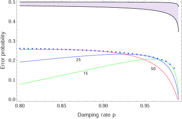
Figure 4: Error probability in the discrimination of two amplitude damping channels, one with damping rate $p\geq 0.8$ and the other with rate $p+1\%$. We assume $n=20$ probings of the unknown channel. The upper dark region identifies the region where the error probability $p_{n}^{\text{block}}$ of Eq. (34) lies. The adaptive error probability $p_{n}(\mathcal{E}_{p_{0}}\neq\mathcal{E}_{p_{1}})$ lies below this dark region and above the dotted points, which represent our lower bound of Eq. (37) optimized over the number of ports $M$. For comparison, we also plot the lower bound for specific $M$.

III Discussion

In this work we have established a general and fundamental lower bound for the error probability affecting the adaptive discrimination of two arbitrary quantum channels acting on a finite-dimensional Hilbert space. This bound is conveniently expressed in terms of the Choi matrices of the channels involved, so that it is very easy to compute. It also applies to many scenarios, including adaptive protocols for quantum-enhance optical resolution and quantum illumination. In order to derive our result, we have employed port-based teleportation as a tool for channel simulation, and developed a methodology which simplifies adaptive protocols performed over an arbitrary finite-dimensional channel. This technique can be applied to many other scenarios. For instance, in quantum metrology we are able to prove that adaptive protocols of quantum channel estimation are limited by a bound simply expressed in terms of the Choi matrix of the channel and following the Heisenberg scaling in the number of probings. Not only this shows that our bound is asymptotically tight but also draws an unexpected connection between port-based teleportation and quantum metrology. Further potential applications are in quantum and private communications, which are briefly discussed in our Supplementary Section V.

IV Methods

IV.1 Simulation error in diamond norm (proof of Lemma 1)

It is easy to check that the channel $\Gamma_{M}$ associated with the qudit PBT protocol of Ref. PBT is covariant under unitary transformations, i.e.,

$$\Gamma_{M}(U\rho U^{{\dagger}})=U\Gamma_{M}(\rho)U^{{\dagger}},$$ (38)

for any input state $\rho$ and unitary operator $U$. As discussed in Ref. Majenz , for a channel with such a symmetry, the diamond distance with the identity map is saturated by a maximally entangled state, i.e.,

$$\|\mathcal{I}-\Gamma_{M}\|_{\diamond}=\||\Phi\rangle\langle\Phi|-\mathcal{I}\otimes\Gamma_{M}\left(|\Phi\rangle\langle\Phi|\right)\|\,,$$ (39)

where $|\Phi\rangle=d^{-1/2}\sum_{k=1}^{d}|k\rangle|k\rangle$. Here we first show that

$$\||\Phi\rangle\langle\Phi|-\mathcal{I}\otimes\Gamma_{M}\left(|\Phi\rangle\langle\Phi|\right)\|=2[1-f_{e}(\Gamma_{M})]~{}.$$ (40)

In fact, note that the map $\Lambda_{M}=\mathcal{I}\otimes\Gamma_{M}$ is covariant under twirling unitaries of the form $U\otimes U^{\ast}$, i.e.,

$$\Lambda_{M}\left[(U\otimes U^{\ast})\rho(U\otimes U^{\ast})^{{\dagger}}\right]$$

$$=(U\otimes U^{\ast})\Lambda_{M}(\rho)(U\otimes U^{\ast})^{{\dagger}},$$ (41)

for any input state $\rho$ and unitary operator $U$. This implies that the state $\Lambda_{M}(|\Phi\rangle\langle\Phi|)$ is invariant under twirling unitaries, i.e.,

$$(U\otimes U^{\ast})\Lambda_{M}(|\Phi\rangle\langle\Phi|)(U\otimes U^{\ast})^{{\dagger}}=\Lambda_{M}(|\Phi\rangle\langle\Phi|)~{}.$$ (42)

This is therefore an isotropic state of the form

$$\Lambda_{M}(|\Phi\rangle\langle\Phi|)=(1-p)|\Phi\rangle\langle\Phi|+\frac{p}{d^{2}}\mathbb{I},$$ (43)

where $\mathbb{I}$ is the two-qudit identity operator.

We may rewrite this state as follows

$$\Lambda_{M}(|\Phi\rangle\langle\Phi|)=F|\Phi\rangle\langle\Phi|+(1-F)\rho^{\perp},$$ (44)

where $\rho^{\perp}$ is state with support in the orthogonal complement of $\Phi$, and $F$ is the singlet fraction

$$F:=\langle\Phi|\Lambda_{M}(|\Phi\rangle\langle\Phi|)|\Phi\rangle=1-p+pd^{-2}.$$ (45)

Thanks to the decomposition in Eq. (44) and using basic properties of the trace norm NiCh , we may then write

$$\||\Phi\rangle\langle\Phi|-\Lambda_{M}\left(|\Phi\rangle\langle\Phi|\right)\|$$

$$=\|(1-F)|\Phi\rangle\langle\Phi|-(1-F)\rho^{\perp}\|$$

$$=(1-F)\||\Phi\rangle\langle\Phi|\|+(1-F)\|\rho^{\perp}\|$$

$$=2(1-F)$$

$$=2[1-f_{e}(\Gamma_{M})],$$ (46)

where the last step exploits the fact that the singlet fraction $F$ is the channel’s entanglement fidelity $f_{e}(\Gamma_{M})$. This completes the proof of Eq. (40).

Therefore, combining Eqs. (39) and (40), we obtain

$$\|\mathcal{I}-\Gamma_{M}\|_{\diamond}=2[1-f_{e}(\Gamma_{M})],$$ (47)

which is Eq. (8) of the main text. Then, we know that the entanglement fidelity of $\Gamma_{M}$ is bounded as PBT

$$f_{e}(\Gamma_{M})\geq 1-d(d-1)M^{-1}.$$ (48)

Therefore, using Eq. (48) in Eq. (47), we derive the following upper bound

$$\|\mathcal{I}-\Gamma_{M}\|_{\diamond}\leq 2d(d-1)M^{-1},$$ (49)

which is Eq. (9) of the main text.

Let us now prove Eq. (10). It is known PBT1 that implementing the standard PBT protocol over the resource state of Eq. (6) leads to a PBT channel $\Gamma_{M}$ which is a qudit depolarizing channel. Its isotropic Choi matrix $\rho_{\Gamma_{M}}$, given in Eq. (43), can be written in the form

$$\rho_{\Gamma_{M}}=\left(1-\frac{d^{2}-1}{d^{2}}\xi_{M}\right)|\Phi\rangle^{0}\langle\Phi|+\sum_{i=1}^{d^{2}-1}\frac{\xi_{M}}{d^{2}}|\Phi\rangle^{i}\langle\Phi|,$$ (50)

where $\xi_{M}$ is the probability $p$ of depolarizing, $|\Phi\rangle^{0}\langle\Phi|$ is the projector onto the initial maximally-entangled state of two qudits (one system of which was sent through the channel), and $|\Phi\rangle^{i}\langle\Phi|$ are the projectors onto the other $d^{2}-1$ maximally-entangled states of two qudits (generalized Bell states). Since the Choi matrix of the identity channel is $\rho_{\mathcal{I}}=|\Phi\rangle^{0}\langle\Phi|$, it is easy to compute

$$\left|\rho_{\mathcal{I}}-\rho_{\Gamma_{M}}\right| :=\sqrt{\left(\rho_{\mathcal{I}}-\rho_{\Gamma_{M}}\right)\left(\rho_{\mathcal{I}}-\rho_{\Gamma_{M}}\right)^{{\dagger}}}$$

$$=\frac{d^{2}-1}{d^{2}}\xi_{M}|\Phi\rangle^{0}\langle\Phi|+\sum_{i=1}^{d^{2}-1}\frac{\xi_{M}}{d^{2}}|\Phi\rangle^{i}\langle\Phi|.$$ (51)

From the previous equation, we derive

$$\mathrm{Tr}_{2}\left|\rho_{\mathcal{I}}-\rho_{\Gamma_{M}}\right|=\frac{2\left(d^{2}-1\right)}{d^{3}}\xi_{M}\sum_{j=0}^{d-1}|j\rangle\langle j|,$$ (52)

where we have used $\mathrm{Tr}_{2}|\Phi\rangle^{i}\langle\Phi|=d^{-1}\sum_{j=0}^{d-1}|j\rangle\langle j|$ in the qudit computational basis $\{|j\rangle\}$ and we have summed over the $d^{2}$ generalized Bell states. It is clear that Eq. (52) is a diagonal matrix with equal non-zero elements, i.e., it is a scalar. As a result, we can apply Proposition 1 of Ref. nechita over the Hermitian operator $\rho_{\mathcal{I}}-\rho_{\Gamma_{M}}$, and write

$$\|\mathcal{I}-\Gamma_{M}\|_{\diamond}=\|\rho_{\mathcal{I}}-\rho_{\Gamma_{M}}\|$$

$$=\mathrm{Tr}\left|\rho_{\mathcal{I}}-\rho_{\Gamma_{M}}\right|=\frac{2\left(d^{2}-1\right)}{d^{2}}\xi_{M}~{}.$$ (53)

The final step of the proof is to compute the explicit expression of $\xi_{M}$ for qubits, which is the formula given in Eq. (11). Because this derivation is technically involved, it is reported in Supplementary Section I.

IV.2 Propagation of the simulation error

For the sake of completeness, we provide the proof of the first inequality in Eq. (15) (this kind of proof already appeared in Refs. PLOB ; TQC ). Consider the adaptive protocol described in the main text. For the $n$-use output state we may compactly write

$$\rho_{n}=\Lambda_{n}\circ\mathcal{E}\circ\Lambda_{n-1}\circ\cdots\circ\mathcal{E}\circ\Lambda_{1}\circ\mathcal{E}(\rho_{0}),$$ (54)

where $\Lambda$’s are adaptive QOs and $\mathcal{E}$ is the channel applied to the transmitted signal system. Then, $\rho_{0}$ is the preparation state of the registers, obtained by applying the first QO$\ \Lambda_{0}$ to some fundamental state. Similarly, for the $M$-port simulation of the protocol, we may write

$$\rho_{n}^{M}=\Lambda_{n}\circ\mathcal{E}^{M}\circ\Lambda_{n-1}\circ\cdots\circ\mathcal{E}^{M}\circ\Lambda_{1}\circ\mathcal{E}^{M}(\rho_{0}),$$ (55)

where $\mathcal{E}^{M}$ is in the place of $\mathcal{E}$.

Consider now two instances ($n=2$) of the adaptive protocol. We may bound the trace distance between $\rho_{2}$ and $\rho_{2}^{M}$ using a “peeling” argument PirCo ; PLOB ; TQC ; Uniform ; ReviewMETRO

$$\left\|\rho_{2}-\rho_{2}^{M}\right\| =\left\|\Lambda_{2}\circ\mathcal{E}\circ\Lambda_{1}\circ\mathcal{E}(\rho_{0})\right.$$

$$-\Lambda_{2}\circ\mathcal{E}^{M}\circ\Lambda_{1}\circ\mathcal{E}^{M}(\rho_{0})||$$

$$\overset{{\tiny(1)}}{\leq}||\mathcal{E}\circ\Lambda_{1}\circ\mathcal{E}(\rho_{0})-\mathcal{E}^{M}\circ\Lambda_{1}\circ\mathcal{E}^{M}(\rho_{0})||$$

$$\overset{{\tiny(2)}}{\leq}||\mathcal{E}\circ\Lambda_{1}\circ\mathcal{E}(\rho_{0})-\mathcal{E}\circ\Lambda_{1}\circ\mathcal{E}^{M}(\rho_{0})||$$

$$+||\mathcal{E}^{M}\circ\Lambda_{1}\circ\mathcal{E}(\rho_{0})-\mathcal{E}^{M}\circ\Lambda_{1}\circ\mathcal{E}^{M}(\rho_{0})||$$

$$\overset{{\tiny(3)}}{\leq}||\mathcal{E}(\rho_{0})-\mathcal{E}^{M}(\rho_{0})||$$

$$+||\mathcal{E}[\Lambda_{1}\circ\mathcal{E}^{M}(\rho_{0})]-\mathcal{E}^{M}[\Lambda_{1}\circ\mathcal{E}^{M}(\rho_{0})]||$$

$$\overset{{\tiny(4)}}{\leq}2||\mathcal{E}-\mathcal{E}^{M}||_{\diamond}~{}.$$ (56)

In $(1)$ we use the monotonicity of the trace distance under completely-positive trace-preserving (CPTP) maps (i.e., quantum channels); in $(2)$ we employ the triangle inequality; in $(3)$ we use the monotonicity with respect to the the CPTP map $\mathcal{E}\circ\Lambda_{1}$ whereas in $(4)$ we exploit the fact that the diamond norm is an upper bound for the trace norm computed on any input state. Generalizing the result of Eq. (56) to arbitrary $n$, we achieve the first inequality in Eq. (15). Note that the previous reasoning also applies to a classically-parametrized channel $\mathcal{E}_{u}$.

IV.3 PBT simulation of amplitude damping channels

Here we show the result in Eq. (36) for $\Delta_{M}(p)=||\mathcal{E}_{p}-\mathcal{E}_{p}^{M}||_{\diamond}$, which is the error associated with the $M$-port simulation of an arbitrary amplitude damping channel $\mathcal{E}_{p}$. From Ref. PBT1 , we know that the PBT channel $\Gamma^{M}$ is a depolarizing channel. In the qubit computational basis $\{\left|i,j\right\rangle\}_{i,j=0,1}$, it has the following Choi matrix

$$\rho_{\Gamma^{M}}=\begin{pmatrix}\frac{1}{2}-\frac{\xi_{M}}{4}&0&0&\frac{1}{2}-\frac{\xi_{M}}{2}\\ 0&\frac{\xi_{M}}{4}&0&0\\ 0&0&\frac{\xi_{M}}{4}&0\\ \frac{1}{2}-\frac{\xi_{M}}{2}&0&0&\frac{1}{2}-\frac{\xi_{M}}{4}\end{pmatrix},$$ (57)

where $\xi_{M}$ are the PBT numbers of Eq. (11). Note that these take decreasing positive values, for instance

$$\xi_{2} =\frac{6-\sqrt{3}}{6}\simeq 0.71,$$

$$\xi_{3} =1/2,$$

$$\xi_{4} =\frac{13-2\sqrt{2}-2\sqrt{5}}{16},$$

$$\xi_{5} =\frac{35-4\sqrt{6}-4\sqrt{10}}{48},$$

$$\xi_{6} =\frac{70-15\sqrt{3}-5\sqrt{7}-3\sqrt{15}}{96}\simeq 0.2.$$ (58)

By applying the Kraus operators $K_{0}$ and $K_{1}$ of $\mathcal{E}_{p}$ locally to $\rho_{\Gamma^{M}}$ we obtain the Choi matrix of the $M$-port simulation $\mathcal{E}_{p}^{M}$, which is

$$\rho_{\mathcal{E}_{p}^{M}}=\begin{pmatrix}x&0&0&y\\ 0&\left(1-p\right)\xi_{M}&0&0\\ 0&0&w&0\\ y&0&0&z\end{pmatrix},$$ (59)

where $x:=\frac{1}{2}-\left(1-p\right)\frac{\xi_{M}}{4}$, $y:=\sqrt{1-p}\left(\frac{1}{2}-\frac{\xi_{M}}{2}\right)$, $z:=\left(\frac{1}{2}-\frac{\xi_{M}}{4}\right)\left(1-p\right)$, and $w:=\left(\frac{1}{2}-\frac{\xi_{M}}{4}\right)p+\frac{\xi_{M}}{4}$. This has to be compared with the Choi matrix of $\mathcal{E}_{p}$, which is

$$\rho_{\mathcal{E}_{p}}=\begin{pmatrix}\frac{1}{2}&0&0&\frac{\sqrt{1-p}}{2}\\ 0&0&0&0\\ 0&0&\frac{p}{2}&0\\ \frac{\sqrt{1-p}}{2}&0&0&\frac{1-p}{2}\end{pmatrix}.$$ (60)

Now, consider the Hermitian matrix $J=\rho_{\mathcal{E}_{p}^{M}}-\rho_{\mathcal{E}_{p}}$. If the matrix $\phi=\mathrm{Tr}_{2}\sqrt{J^{{\dagger}}J}=\mathrm{Tr}_{2}\sqrt{JJ^{{\dagger}}}$ is scalar (i.e., both of its eigenvalues are equal), then the trace distance between the Choi matrices $||J||$ is equal to the diamond distance between the channels $\Delta_{M}(p)$ (nechita, , Proposition 1). After simple algebra we indeed find

$$\phi=\frac{\xi_{M}}{8}\left[2(1-p)+a_{-}+a_{+}\right]\begin{pmatrix}1&0\\ 0&1\end{pmatrix},$$ (61)

where $a_{\pm}=\sqrt{1-p}\sqrt{5\pm 4\sqrt{1-p}-p}$. Because $\phi$ is scalar, the condition above is met and the expression of $\Delta_{M}(p)$ is twice the (degenerate) eigenvalue of $\phi$, i.e.,

$$\Delta_{M}(p)=\frac{\xi_{M}}{4}\left[2(1-p)+a_{-}+a_{+}\right],$$ (62)

which simplifies to Eq. (36).

Aknowledgements

This work has been supported by the EPSRC via the ‘UK Quantum Communications Hub’ (EP/M013472/1) and by the European Commission via ‘Continuous Variable Quantum Communications’ (CiViQ, Project ID: 820466). The authors would like to thank Satoshi Ishizaka, Sam Braunstein, Seth Lloyd, Gaetana Spedalieri, and Zhi-Wei Wang for feedback.

Supplementary Information

I Depolarizing probability for qubit PBT

Here we show the formula for the PBT numbers $\xi_{M}$ given in Eq. (11) of the main text. Define the states

$$|\phi^{-}\rangle =\left(|01\rangle-|10\rangle\right)/\sqrt{2},$$ (63)

$$\sigma^{i} =\frac{1}{2^{M-1}}|\phi^{-}\rangle\langle\phi^{-}|_{A_{i}C}\otimes\mathbb{I}_{\mathbf{\bar{A}}}^{M-1},$$ (64)

$$\rho =\sum_{i=1}^{M}\sigma^{i},$$ (65)

where $\mathbb{I}_{\mathbf{\bar{A}}}^{M-1}$ is the $2^{M-1}$-dimensional identity operator acting on the $M-1$ qubits $\mathbf{\bar{A}}=\mathbf{A}\backslash A_{i}$ (similarly, we denote $\mathbf{\bar{B}}=\mathbf{B}\backslash B_{i}$). Then, in qubit-based PBT with $M$ ports, one uses a POVM with operators

$$\Pi_{C\mathbf{A}}^{i}=\rho^{-\frac{1}{2}}\sigma^{i}\rho^{-\frac{1}{2}}+M^{-1}\left(\mathbb{I}^{M+1}-\rho^{-\frac{1}{2}}\rho\rho^{-\frac{1}{2}}\right),$$ (66)

where $\mathbb{I}^{M+1}$ is the $2^{M+1}$-dimensional identity operator acting on the input qubit $C$ and Alice’s resource qubits $\mathbf{A}$, while $\rho^{-\frac{1}{2}}$ is taken over the support of $\rho$ PBT1s .

Since the resource state

$$\Phi_{\mathbf{AB}}^{\otimes M}=\bigotimes_{i=1}^{M}|\phi^{-}\rangle_{i}\langle\phi^{-}|$$ (67)

is symmetric under exchange of labels, we can calculate $\xi_{M}$ assuming that the qubit is teleported to the first port, and hence we only need to consider $\Pi_{C\mathbf{A}}^{1}$. The PBT channel $\Gamma_{M}$ from qubit $C$ to qubit $B_{1}$ is a depolarizing channel with isotropic Choi matrix

$$(\rho_{\Gamma_{M}})_{DB_{1}}=\begin{pmatrix}\frac{1}{2}-\frac{\xi_{M}}{4}&0&0&\frac{1}{2}-\frac{\xi_{M}}{2}\\ 0&\frac{\xi_{M}}{4}&0&0\\ 0&0&\frac{\xi_{M}}{4}&0\\ \frac{1}{2}-\frac{\xi_{M}}{2}&0&0&\frac{1}{2}-\frac{\xi_{M}}{4}\end{pmatrix},$$ (68)

where $\xi_{M}$ is the probability of depolarizing and $D$ is the ancillary system not passing through the PBT channel. Note that we can equivalently use a POVM $\{\Pi_{C\mathbf{A}}^{i}\}$ and a resource state $\Phi_{\mathbf{AB}}^{\otimes M}$ where we replace

$$|\phi^{-}\rangle\rightarrow|\Phi\rangle=\left(|00\rangle+|11\rangle\right)/\sqrt{2}.$$ (69)

In order to find $\xi_{M}$, it suffices to find any one of the non-zero elements in the output Choi matrix. Selecting the coefficient of $|01\rangle_{DB_{1}}\langle 01|$, our expression is

$$\frac{\xi_{M}}{4M} =\langle 01|\mathrm{Tr}_{\mathbf{A\bar{B}}C}\left[\sqrt{\Pi^{1}}\Phi_{\mathbf{AB}}^{\otimes M}|\Phi\rangle_{CD}\langle\Phi|\sqrt{\Pi^{1}}\right]|01\rangle$$ (70)

$$=\mathrm{Tr}\left[\Pi_{C\mathbf{A}}^{1}\Phi_{\mathbf{AB}}^{\otimes M}|\Phi\rangle_{CD}\langle\Phi||01\rangle_{DB_{1}}\langle 01|\right]$$ (71)

$$=\tfrac{1}{2}\mathrm{Tr}\left[\Pi_{C\mathbf{A}}^{1}\langle 1|_{B_{1}}\mathrm{Tr}_{\mathbf{\bar{B}}}(\Phi_{\mathbf{AB}}^{\otimes M})|1\rangle_{B_{1}}\otimes|0\rangle_{C}\langle 0|\right],$$ (72)

where the factor of $M$ comes from the fact we have $M$ possible outcomes and where the third line is due to $|\Phi\rangle_{CD}$. Considering the structure of $\Phi_{\mathbf{AB}}^{\otimes M}$, we can write

$$\xi_{M}=\frac{M}{2^{M-1}}\mathrm{Tr}\left[\Pi_{C\mathbf{A}}^{1}\left(\mathbb{I}_{\mathbf{\bar{A}}}^{M-1}\otimes|00\rangle_{A_{1}C}\langle 00|\right)\right].$$ (73)

Ref. PBT1s showed that, by using a spinorial basis, the eigenvectors and eigenvalues of $\rho$ can be expressed in a simple form. Defining the basis vectors $\{|\Phi^{M}(j,m,\alpha)\rangle\}$, where $j$ is the total spin, $m$ is the spin component in the z-basis and $\alpha$ is a degeneracy value, they constructed the eigenvectors of $\rho$ as

$$|\Psi(\lambda_{j}^{\mp},m,\alpha)\rangle=$$ (74)

$$|\Phi^{M}(j,m+\frac{1}{2},\alpha)\rangle_{\mathbf{A}}|0\rangle_{C}\left\langle j,m+\frac{1}{2},\frac{1}{2},-\frac{1}{2}\middle|j\pm\frac{1}{2},m\right\rangle$$

$$+|\Phi^{M}(j,m-\frac{1}{2},\alpha)\rangle_{\mathbf{A}}|1\rangle_{C}\left\langle j,m-\frac{1}{2},\frac{1}{2},\frac{1}{2}\middle|j\pm\frac{1}{2},m\right\rangle,$$

where the terms in the large, triangular brackets are the Clebsch-Gordan coefficients. They found that these eigenvectors correspond to the eigenvalues

$$\lambda_{j}^{-}=\frac{1}{2}\left(\frac{M}{2}-j\right),~{}\lambda_{j}^{+}=\frac{1}{2}\left(\frac{M}{2}+j+1\right).$$ (75)

(Our expressions differ from those in Ref. PBT1s by a factor of $2^{M+1}$ due to including this factor in the definition of the $\sigma^{i}$). Then, Ref. PBT1s expressed the state $\rho$ as

$$\rho =\sum_{s,m,\alpha}\lambda_{j}^{-}|\Psi(\lambda_{s-\frac{1}{2}}^{-},m,\alpha)\rangle\langle\Psi(\lambda_{s-\frac{1}{2}}^{-},m,\alpha)|$$

$$+\lambda_{j}^{+}|\Psi(\lambda_{s+\frac{1}{2}}^{+},m,\alpha)\rangle\langle\Psi(\lambda_{s+\frac{1}{2}}^{+},m,\alpha)|.$$ (76)

Note that the basis vectors on an $M$-spin system, $\{|\Phi^{M}(j,m,\alpha)\rangle\}$, can be divided into two types based on how they are constructed from the basis vectors on an $(M-1)$-spin system, $\{|\Phi^{M-1}(j,m,\alpha)\rangle\}$. Specifically

$$|\Phi_{I}^{M}(j,m)\rangle=$$ (77)

$$|\Phi^{M-1}(j+\frac{1}{2},m+\frac{1}{2})\rangle|0\rangle\left\langle j+\frac{1}{2},m+\frac{1}{2},\frac{1}{2},-\frac{1}{2}\middle|j,m\right\rangle$$

$$+|\Phi^{M-1}(j+\frac{1}{2},m-\frac{1}{2})\rangle|1\rangle\left\langle j+\frac{1}{2},m-\frac{1}{2},\frac{1}{2},\frac{1}{2}\middle|j,m\right\rangle,$$

and

$$|\Phi_{II}^{M}(j,m)\rangle=$$ (78)

$$|\Phi^{M-1}(j-\frac{1}{2},m+\frac{1}{2})\rangle|0\rangle\left\langle j-\frac{1}{2},m+\frac{1}{2},\frac{1}{2},-\frac{1}{2}\middle|j,m\right\rangle$$

$$+|\Phi^{M-1}(j-\frac{1}{2},m-\frac{1}{2})\rangle|1\rangle\left\langle j-\frac{1}{2},m-\frac{1}{2},\frac{1}{2},\frac{1}{2}\middle|j,m\right\rangle,$$

where we have omitted the label $\alpha$, but both component vectors are assumed to have the same degeneracy value. We also divide the eigenvectors $\{|\Psi(\lambda_{j}^{\mp},m,\alpha)\rangle\}$ into types $I$ and $II$, based on whether they are constructed from the vectors $\{|\Phi_{I}^{M}(j,m,\alpha)\rangle\}$ or $\{|\Phi_{II}^{M}(j,m,\alpha)\rangle\}$. Ref. PBT1s also used the explicit forms of the Clebsch-Gordon coefficients to calculate the expressions

$$\langle\phi^{-}|_{A_{1}C}|\Psi_{I}(\lambda_{s}^{-}-\frac{1}{2},m,\alpha)\rangle_{\mathbf{A}C}=$$

$$\sqrt{\frac{s}{2s+1}}|\Phi^{M-1}(s,m,\alpha)\rangle_{\mathbf{\bar{A}}}$$ (79)

$$\langle\phi^{-}|_{A_{1}C}|\Psi_{I}(\lambda_{s}^{+}+\frac{1}{2},m,\alpha)\rangle_{\mathbf{A}C}=0,$$ (80)

$$\langle\phi^{-}|_{A_{1}C}|\Psi_{II}(\lambda_{s}^{-}-\frac{1}{2},m,\alpha)\rangle_{\mathbf{A}C}=0,$$ (81)

$$\langle\phi^{-}|_{A_{1}C}|\Psi_{II}(\lambda_{s}^{+}+\frac{1}{2},m,\alpha)\rangle_{\mathbf{A}C}=$$

$$-\sqrt{\frac{s+1}{2s+1}}|\Phi^{M-1}(s,m,\alpha)\rangle_{\mathbf{\bar{A}}}.$$ (82)

We can express $\sigma^{1}$as

$$\sigma^{1}=|\phi^{-}\rangle_{A_{1}C}\langle\phi^{-}|\otimes$$

$$\sum_{j=j_{min}}^{\frac{M-1}{2}}\sum_{m=-j}^{j}\sum_{\alpha}|\Phi^{M-1}(j,m,\alpha)\rangle_{\mathbf{\bar{A}}}\langle\Phi^{M-1}(j,m,\alpha)|$$ (83)

where the term over the $\mathbf{\bar{A}}$ qubits is the identity. We now separate out the contributions from the two terms of $\Pi^{1}$, writing

$$\Pi^{1} =\pi_{0}+\pi_{1},$$ (84)

$$\pi_{0} =M^{-1}\left(\mathbb{I}^{M+1}-\rho^{-\frac{1}{2}}\rho\rho^{-\frac{1}{2}}\right),$$ (85)

$$\pi_{1} =\rho^{-\frac{1}{2}}\sigma^{1}\rho^{-\frac{1}{2}}.$$ (86)

Here $\pi_{0}$ is simply $M^{-1}$ times the identity over the vector space that does not lie in the support of $\rho$, and corresponds to those eigenvectors of $\rho$ with eigenvalue 0, namely $\{|\Psi_{II}(\lambda_{\frac{M}{2}}^{-},m)\rangle\}$ (omitting the label $\alpha$, since the degeneracy is $1$ for this choice of $j$). Consequently, we may write

$$\pi_{0}=M^{-1}\sum_{m=-\frac{M+1}{2}}^{\frac{M+1}{2}}|\Psi_{II}(\lambda_{\frac{M}{2}}^{-},m)\rangle\langle\Psi_{II}(\lambda_{\frac{M}{2}}^{-},m)|.$$ (87)

Combining the expressions for $\rho$ and $\sigma^{1}$ in Eqs. (76) and (83) and the expressions in Eqs. (79)-(82), we can write

$$\pi_{1} =\sum_{s=s_{min}}^{(M-1)/2}\sum_{m=-s}^{s}\sum_{\alpha}$$ (88)

$$\left[(\lambda_{s-\frac{1}{2}}^{-})^{-1}\frac{s}{2s+1}|\Psi_{I}(\lambda_{s-\frac{1}{2}}^{-},m,\alpha)\rangle\langle\Psi_{I}(\lambda_{s-\frac{1}{2}}^{-},m,\alpha)|\right.$$

$$-(\lambda_{s-\frac{1}{2}}^{-}\lambda_{s+\frac{1}{2}}^{+})^{-\frac{1}{2}}\frac{\sqrt{s(s+1)}}{2s+1}$$

$$\left(|\Psi_{I}(\lambda_{s-\frac{1}{2}}^{-},m,\alpha)\rangle\langle\Psi_{II}(\lambda_{s+\frac{1}{2}}^{+},m,\alpha)|+\right.$$

$$\left.|\Psi_{II}(\lambda_{s+\frac{1}{2}}^{+},m,\alpha)\rangle\langle\Psi_{I}(\lambda_{s-\frac{1}{2}}^{-},m,\alpha)|\right)+$$

$$\left.(\lambda_{s+\frac{1}{2}}^{+})^{-1}\frac{s+1}{2s+1}|\Psi_{II}(\lambda_{s+\frac{1}{2}}^{+},m,\alpha)\rangle\langle\Psi_{II}(\lambda_{s+\frac{1}{2}}^{+},m,\alpha)|\right],$$

where $s_{min}=1/2$ for even $M$, and $0$ for odd $M$.

By calculating the Clebsch-Gordan coefficients, we find

$$\langle\Psi_{I}(\lambda_{s-\frac{1}{2}}^{-},m)|(\mathbb{I}^{M-1}\otimes|00\rangle\langle 00|)|\Psi_{I}(\lambda_{s-\frac{1}{2}}^{-},m)\rangle=$$

$$\frac{(s-m)(s+m+1)}{2s(2s+1)},$$ (89)

$$\langle\Psi_{II}(\lambda_{s+\frac{1}{2}}^{+},m)|(\mathbb{I}^{M-1}\otimes|00\rangle\langle 00|)|\Psi_{II}(\lambda_{s+\frac{1}{2}}^{+},m)\rangle=$$

$$\frac{(s-m)(s+m+1)}{2(s+1)(2s+1)},$$ (90)

$$\langle\Psi_{I}(\lambda_{s-\frac{1}{2}}^{-},m)|(\mathbb{I}^{M-1}\otimes|00\rangle\langle 00|)|\Psi_{II}(\lambda_{s+\frac{1}{2}}^{+},m)\rangle=$$

$$\frac{(s-m)(s+m+1)}{2(2s+1)\sqrt{s(s+1)}},$$ (91)

$$\langle\Psi_{II}(\lambda_{\frac{M}{2}}^{-},m)|(\mathbb{I}^{M-1}\otimes|00\rangle\langle 00|)|\Psi_{II}(\lambda_{\frac{M}{2}}^{-},m)\rangle=$$

$$\frac{M-1-2m}{2M}\left(\frac{1}{2}-\frac{m}{M+1}\right).$$ (92)

Using Eq. (92) and summing over $m$, we find

$$\frac{M}{2^{M-1}}\mathrm{Tr}\left[\pi_{0}\left(\mathbb{I}_{\mathbf{\bar{A}}}^{M-1}\otimes|01\rangle_{A_{1}C}\langle 01|\right)\right]=\frac{1}{3}\frac{M+2}{2^{M-1}}.$$ (93)

Using Eqs. (89)-(91), we find

$$\frac{M}{2^{M-1}}\mathrm{Tr}\left[\pi_{1}\left(\mathbb{I}_{\mathbf{\bar{A}}}^{M-1}\otimes|01\rangle_{A_{1}C}\langle 01|\right)\right]=$$

$$\frac{M}{2^{M-1}}\sum_{s=s_{min}}^{(M-1)/2}\sum_{m=-s}^{s}\sum_{\alpha}\frac{(s-m)(s+m+1)}{2(2s+1)^{2}}$$

$$\times\left[(\lambda_{s-\frac{1}{2}}^{-})^{-1}-2(\lambda_{s-\frac{1}{2}}^{-}\lambda_{s+\frac{1}{2}}^{+})^{-\frac{1}{2}}+(\lambda_{s+\frac{1}{2}}^{+})^{-1}\right].$$ (94)

We can simplify the term on the RHS, using

$$\left[(\lambda_{s-\frac{1}{2}}^{-})^{-1}-2(\lambda_{s-\frac{1}{2}}^{-}\lambda_{s+\frac{1}{2}}^{+})^{-\frac{1}{2}}+(\lambda_{s+\frac{1}{2}}^{+})^{-1}\right]$$

$$=\left[(\lambda_{s-\frac{1}{2}}^{-})^{-\frac{1}{2}}-(\lambda_{s+\frac{1}{2}}^{+})^{-\frac{1}{2}}\right]^{2}.$$ (95)

The degeneracy g$[s]$ for a given $s$-value is given by

$$\mathrm{g}[s]=\frac{(2s+1)(M-1)!}{\left(\frac{M-1}{2}-s\right)!\left(\frac{M+1}{2}+s\right)!},$$ (96)

and substituting this into Eq. (94), we get

$$\frac{M}{2^{M-1}}\mathrm{Tr}\left[\pi_{1}\left(\mathbb{I}_{\mathbf{\bar{A}}}^{M-1}\otimes|01\rangle_{A_{1}C}\langle 01|\right)\right]=$$

$$\sum_{s=s_{min}}^{(M-1)/2}\sum_{m=-s}^{s}\frac{(s-m)(s+m+1)}{2^{M}(2s+1)}\binom{M}{\frac{M-1}{2}-s}$$

$$\times 8\frac{\left(M+2\right)-\sqrt{\left(M+2\right)^{2}-\left(2s+1\right)^{2}}}{\left(M+2\right)^{2}-\left(2s+1\right)^{2}},$$ (97)

where we have substituted in the expressions from Eq. (75). Summing over $m$, we get

$$\frac{M}{2^{M-1}}\mathrm{Tr}\left[\pi_{1}\left(\mathbb{I}_{\mathbf{\bar{A}}}^{M-1}\otimes|01\rangle_{A_{1}C}\langle 01|\right)\right]=$$

$$\sum_{s=s_{min}}^{(M-1)/2}\frac{1}{3}\frac{s(s+1)}{2^{M-4}}\binom{M}{\frac{M-1}{2}-s}$$

$$\times\frac{\left(M+2\right)-\sqrt{\left(M+2\right)^{2}-\left(2s+1\right)^{2}}}{\left(M+2\right)^{2}-\left(2s+1\right)^{2}}.$$ (98)

Therefore, by combining Eqs. (93) and (98), we finally get the expression of $\xi_{M}$ given in Eq. (11) of the main text. We can numerically verify that $\xi_{M}$ scales as $M^{-1}$ for large $M$.

One may check that Eq. (11) of the main text can equivalently be obtained by combining Eq. (47) of our Methods section (i.e., Eq. (8) of our Lemma 1) together with the expression of the entanglement fidelity for qubit-based PBT which is given in Eq. (29) of Ref. PBT1s . For completeness we report this algebraic check here.

We start from the expression of $\xi_{M}$ given in Eq. (11) of the main text. By substituting this expression in Eq. (10) of the main text for $d=2$, we get

$$\begin{split}\delta_{M}&=\frac{3}{2}\xi_{M}\\ &=\frac{M+2}{2^{M}}+\sum_{s=s_{min}}^{(M-1)/2}\frac{s(s+1)}{2^{M-3}}\binom{M}{\frac{M-1}{2}-s}\times\\ &\frac{\left(M+2\right)-\sqrt{\left(M+2\right)^{2}-\left(2s+1\right)^{2}}}{\left(M+2\right)^{2}-\left(2s+1\right)^{2}}.\end{split}$$ (99)

We now use the fact that each term in the sum would be the same if we set $s$ to $-(s+1)$, and write

$$\begin{split}\delta_{M}&=\frac{M+2}{2^{M}}+\sum_{s=-(M+1)/2}^{(M-1)/2}\frac{s(s+1)}{2^{M-2}}\binom{M}{\frac{M-1}{2}-s}\times\\ &\frac{\left(M+2\right)-\sqrt{\left(M+2\right)^{2}-\left(2s+1\right)^{2}}}{\left(M+2\right)^{2}-\left(2s+1\right)^{2}}.\end{split}$$ (100)

Then, we carry out a change of variables, substituting in $k=\frac{M-1}{2}-s$, and get

$$\begin{split}\delta_{M}&=\frac{M+2}{2^{M}}+\sum_{k=0}^{M}\frac{(M-2k-1)(M-2k+1)}{2^{M}}\binom{M}{k}\times\\ &\frac{\left(M+2\right)-\sqrt{\left(M+2\right)^{2}-\left(M-2k\right)^{2}}}{\left(M+2\right)^{2}-\left(M-2k\right)^{2}}.\end{split}$$ (101)

Using

$$(M+2)^{2}-(M-2k)^{2}=4(M-k+1)(k+1),$$ (102)

we write

$$\begin{split}\delta_{M}&=\frac{M+2}{2^{M}}+\sum_{k=0}^{M}\frac{(M-2k)^{2}-1}{2^{M+2}}\binom{M}{k}\times\\ &\frac{(M+2)-2\sqrt{(M-k+1)(k+1)}}{(M-k+1)(k+1)}.\end{split}$$ (103)

We now use the expression for the entanglement fidelity of qubit PBT given in PBT1s , i.e.,

$$f_{e}=\frac{1}{2^{M+3}}\sum_{k=0}^{M}\left(\frac{M-2k-1}{\sqrt{k+1}}+\frac{M-2k+1}{\sqrt{M-k+1}}\right)^{2}\binom{M}{k}.$$ (104)

Combining this with Eq. (103) and expanding the term in brackets, we can write

$$\begin{split}&f_{e}+\frac{\delta_{M}}{2}=\frac{M+2}{2^{M+1}}+\sum_{k=0}^{M}\frac{2^{-(M+3)}}{(M-k+1)(k+1)}\binom{M}{k}\times\\ &\left[\left((M-2k)^{2}-1\right)\left((M+2)-2\sqrt{(M-k+1)(k+1)}\right)\right.\\ &\left.+\left(M+2+M(M-2k)^{2}+2\left((M-2k)^{2}-1\right)\times\right.\right.\\ &\left.\left.\sqrt{(M-k+1)(k+1)}\right)\right].\end{split}$$ (105)

Algebraically simplifying the term in the square brackets, we get

$$f_{e}+\frac{\delta_{M}}{2}=\frac{M+2}{2^{M+1}}+\sum_{k=0}^{M}\frac{(M-2k)^{2}}{2^{M+2}(M+2)}\binom{M+2}{k+1},$$ (106)

and changing variables again, substituting in $x=k+1$, we can write

$$f_{e}+\frac{\delta_{M}}{2} =\sum_{x=0}^{M+2}\frac{(M+2-2x)^{2}}{2^{M+2}(M+2)}\binom{M+2}{x},$$ (107)

where we have split the term outside the sum into the contributions for the $x=0$ and $x=M+2$ cases. We now use the known sums of binomial coefficients,

$$\begin{split}&\sum_{x=0}^{n}\binom{n}{x}=2^{n},~{}~{}~{}\sum_{x=0}^{n}x\binom{n}{x}=n2^{n-1},\\ &\sum_{x=0}^{n}x^{2}\binom{n}{x}=(n+n^{2})2^{n-2},\end{split}$$ (108)

and split the sum in Eq. (107) into contributions from $(M+2)^{2}$, $(2x)(M+2)$ and $(2x)^{2}$, getting

$$\begin{split}f_{e}+\frac{\delta_{M}}{2}&=\frac{2^{-(M+2)}}{M+2}\left(2^{M+2}(M+2)^{2}-2^{M+3}(M+2)^{2}\right.\\ &\left.+2^{M+2}\left((M+2)+(M+2)^{2}\right)\right),\end{split}$$ (109)

which cancels to give $f_{e}+\frac{\delta_{M}}{2}=1$, in agreement with $\delta_{M}=2(1-f_{e})$. This check is equivalent to say that, by using Eq. (104) together with Eq. (8) of the main text, we can equivalently obtain Eq. (11) of the main text (specifically for qubits).

II Ultimate single-photon quantum optical resolution

Consider the problem of discriminating between the following situations:

(1)

A point-like source emitting light from position $x=s/2$;

(2)

A point-like source emitting light from the shifted position $x=-s/2$.

The discrimination is achieved by measuring the image created by a focusing optical system. More precisely, we consider a linear imaging system in the paraxial approximation that is used to image point-like sources. This is characterized by the Fresnel number

$$\mathcal{F}=\frac{\ell}{x_{R}}\,,$$ (110)

where $\ell$ is the size of the object, and

$$x_{R}=\frac{\lambda}{N_{A}}$$ (111)

is the Rayleigh length. Here $\lambda$ is the wavelength and $N_{A}=R/D$ is the numerical aperture, where $R$ is the radius of the pupil and $D$ is the distance from the object. In the far-field regime, light is attenuated by a loss parameter $\eta\simeq\mathcal{F}$ Shap ; m1 ; m2 . In particular, because we consider point-like sources, we are in the regime $\eta\ll 1$.

First we need to model the imaging system as a quantum channel acting on the input state represented by the light emitted by the source. The two cases are described by the following Heisenberg-picture transformations on the input annihilation operator $a$

$$(1) :~{}a\rightarrow\sqrt{\eta}b_{1}+\sqrt{1-\eta}v_{1},$$ (112)

$$(2) :~{}a\rightarrow\sqrt{\eta}b_{2}+\sqrt{1-\eta}v_{2},$$ (113)

where $b_{1,2}$ are the output operators (encoding the position of the source) and $v_{1,2}$ are associated with a vacuum environment. The modes $b_{1}$, $b_{2}$ are defined on the image plane and have the form

$$b_{j}=\int dx\,\psi_{j}(x)\,a(x)\,,$$ (114)

where $a(x),a(x)^{{\dagger}}$ is a continuous family of canonical operators $[a(x),a(y)^{{\dagger}}]=\delta(x-y)$ defined on the image plane (for simplicity, we assume unit magnification factor). In general the image modes $b_{1}$, $b_{2}$ do satisfy the (non-canonical) commutation relations

$$[b_{1},b_{2}^{{\dagger}}]=\int dx\,\psi_{1}(x)\psi_{2}^{\ast}(x)\,,$$ (115)

where $\psi_{j}$ is the point-spread function associated to the source being in poisiton $j$. Then, by setting $\delta=\mathrm{Re}\int dx\,\psi_{1}(x)\psi_{2}^{\ast}(x)$, we can define the effective image operators

$$b_{\pm}:=(b_{1}\pm b_{2})/\sqrt{2(1\pm\delta)}.$$ (116)

The fact that $\delta\neq 0$ means that the two image fields overlap and the sources cannot be perfectly distinguished. This is a manifestation of diffraction through the finite objective of the optical imaging system.

As a result, we can write the action of the channels as

$$(1) :~{}a\rightarrow\sqrt{\eta_{+}}b_{+}+\sqrt{\eta_{-}}b_{-}+\sqrt{1-\eta}v_{1},$$ (117)

$$(2) :~{}a\rightarrow\sqrt{\eta_{+}}b_{+}-\sqrt{\eta_{-}}b_{-}+\sqrt{1-\eta}v_{2},$$ (118)

where $\eta_{\pm}:=(1\pm\delta)\eta/2$. For simplicity, consider a single-photon state at the input. We then have

$$(1):~{}|1\rangle \rightarrow\eta|\psi_{+}\rangle\langle\psi_{+}|+(1-\eta)|0\rangle\langle 0|\,,$$ (119)

$$(2):~{}|1\rangle \rightarrow\eta|\psi_{-}\rangle\langle\psi_{-}|+(1-\eta)|0\rangle\langle 0|\,,$$ (120)

where

$$|\psi_{\pm}\rangle=\frac{\sqrt{\eta_{+}}|1\rangle_{+}-\sqrt{\eta_{-}}|1\rangle_{-}}{\sqrt{\eta}}~{}.$$ (121)

More generally, the action of the channels on a generic pure input state is given by

$$(1):~{}\alpha|0\rangle+\beta|1\rangle \rightarrow\left(|\alpha|^{2}+\eta|\beta|^{2}\right)\times$$ (122)

$$|\psi_{+}(\alpha,\beta)\rangle\langle\psi_{+}(\alpha,\beta)|+(1-\eta)|\beta|^{2}|0\rangle\langle 0|,$$

$$(2):~{}\alpha|0\rangle+\beta|1\rangle \rightarrow\left(|\alpha|^{2}+\eta|\beta|^{2}\right)\times$$ (123)

$$|\psi_{-}(\alpha,\beta)\rangle\langle\psi_{-}(\alpha,\beta)|+(1-\eta)|\beta|^{2}|0\rangle\langle 0|,$$

where

$$|\psi_{\pm}(\alpha,\beta)\rangle=\frac{\alpha|0\rangle+\beta\sqrt{\eta_{+}}|1\rangle_{+}\pm\beta\sqrt{\eta_{-}}|1\rangle_{-}}{\sqrt{|\alpha|^{2}+\eta|\beta|^{2}}}~{}.$$ (124)

As we can see from Eqs. (122) and (123), if we apply a Pauli operator $X$ NiChs to the input state $\alpha|0\rangle+\beta|1\rangle$, we have a swap between $\alpha$ and $\beta$. This leads to an output state with a different eigenspectrum, so that it cannot be obtained by applying a unitary. This means that the quantum channels are not teleportation-covariant.

By limiting ourselves to the space of either no photon or one photon $\mathcal{H}_{2}=\mathrm{span}\{|0\rangle,|1\rangle\}$, the the input space of the channels is a qubit, and their output is a qutrit, so that the dimension of the input Hilbert space is $d=2$. Apart from restricting the input space to qubits, we assume the most general adaptive strategy allowed by quantum mechanics, so that the quantum state of the source may be optimized as a consequence of the output (as generally happens in the adaptive protocol discussed in the main text). In order to compute the ultimate performance, we need to compute the quantum fidelity between the Choi matrices of the two channels in Eqs. (117) and (118) suitably truncated to $\mathcal{H}_{2}$.

Consider then the maximally entangled state $|\Phi_{2}\rangle=(|0\rangle|1\rangle+|1\rangle|0\rangle)/\sqrt{2}$. The Choi matrices associated with the two truncated channels are equal to

$$\rho_{(1)} =\frac{1+\eta}{2}|\Psi_{+}\rangle\langle\Psi_{+}|+\frac{1-\eta}{2}|0\rangle\langle 0|\,,$$ (125)

$$\rho_{(2)} =\frac{1+\eta}{2}|\Psi_{-}\rangle\langle\Psi_{-}|+\frac{1-\eta}{2}|0\rangle\langle 0|\,,$$ (126)

where

$$|\Psi_{\pm}\rangle=\frac{|0\rangle|1\rangle+\sqrt{\eta_{+}}|1\rangle_{+}|0\rangle\pm\sqrt{\eta_{-}}|1\rangle_{-}|0\rangle}{\sqrt{1+\eta}}.$$ (127)

Notice that $\langle\Psi_{+}|\Psi_{-}\rangle=(1+\delta\eta)/(1+\eta)$ where $\delta\eta:=\eta_{+}-\eta_{-}$. Therefore we obtain the fidelity

$$F(\rho_{(1)},\rho_{(2)}) =\mathrm{Tr}\sqrt{\sqrt{\rho_{(1)}}\,\rho_{(2)}\,\sqrt{\rho_{(1)}}}$$ (128)

$$=\frac{1+\eta}{2}\left|\frac{1+\delta\eta}{1+\eta}\right|+\frac{1-\eta}{2}=\frac{1-\eta+|1+\delta\eta|}{2}.$$

Assuming that $\delta$ is real, this becomes

$$F[\rho_{(1)},\rho_{(2)}]=1-\frac{\eta(1-\delta)}{2},$$ (129)

which allows us to identify $\epsilon=\eta(1-\delta)/2$. A common way to model diffraction is to consider a Gaussian point-spread function, i.e.

$$\psi_{j}(s)\simeq e^{-(x-x_{j})^{2}/4},$$ (130)

where $x_{j}$ is the center of the $j$th emitter, and the variance of the Gaussian is $1$ in units of Rayleigh length. Under this Gaussian model one obtains Tsang15s ; Lupo16s

$$\delta\simeq e^{-s^{2}/8},$$ (131)

where $s$ is the separation in unit of wavelength. Therefore

$$\epsilon\simeq\frac{\eta(1-e^{-s^{2}/8})}{2}\simeq\frac{\eta s^{2}}{16}.$$ (132)

By replacing this quantity in Eq. (27) of the main text with $d=2$ we obtain the lower bound

$$B\gtrsim\frac{1}{4}\exp{\left(-2ns\sqrt{\eta}\right)}~{}.$$ (133)

III Ultimate limit of adaptive quantum illumination

III.1 Standard (non-adaptive) protocol

In quantum illumination Qill0s ; Qill1s ; Qill2s ; Qill3s , we aim at determining whether a low-reflectivity object is present or not in a region with thermal noise. We therefore prepare a signal system $s$ and an idler system $i$ in a joint entangled state $\rho_{si}$. The signal system is sent to probe the target while the idler system is retained for its measurement together with the potential signal reflection from the target. If the object is absent, the “reflected” system is just thermal background noise. If the object is present, then this is composed of the actual reflection of the signal from the target plus thermal background noise. This object can be modelled by a beam splitter, with very small transmissivity $\eta\ll 1$, which combines the each incoming optical mode (signal system) with a thermal mode with $b$ mean number of photons.

In the discrete-variable version of quantum illumination Qill0s , the signal system is prepared in an ensemble of $d$ optical modes, with $1$ photon in one of the modes and vacuum in the others. This is the number of modes which are distinguished by the detector in each detection process. If we introduce the following $d-$dimensional computational basis

$$\left|1\right\rangle :=\overset{d}{\overbrace{\left|00\ldots 01\right\rangle}},$$ (134)

$$\left|2\right\rangle :=\left|00\ldots 10\right\rangle,$$ (135)

$$\vdots$$

$$\left|d-1\right\rangle :=\left|01\ldots 00\right\rangle,$$ (136)

$$\left|d\right\rangle :=\left|10\ldots 00\right\rangle,$$ (137)

then the entangled signal-idler state can be written as

$$\psi_{si}=|\psi\rangle_{si}\left\langle\psi\right|,~{}~{}|\psi\rangle_{si}=d^{-1/2}\sum_{k=1}^{d}|kk\rangle_{si}~{}.$$ (138)

Let us define the $d$-dimensional identity operator $\mathbb{I}^{d}:=\sum_{k=1}^{d}|k\rangle\left\langle k\right|$ which projects onto the subspace spanned by the $1$-photon states, and the $(d+1)$-dimensional identity operator $\mathbb{I}^{d+1}:=\sum_{k=0}^{d}|k\rangle\left\langle k\right|$ which also includes the vacuum state $\left|0\right\rangle:=\left|00\ldots 00\right\rangle$. Then, we have the reduced idler state

$$\psi_{i}:=\mathrm{Tr}_{s}(\psi_{si})=d^{-1}\mathbb{I}_{i}^{d},$$ (139)

and we define the thermal state of the environment as Qill0s

$$\rho^{\text{th}}(b):=(1-db)|0\rangle\langle 0|+b\mathbb{I}^{d},$$ (140)

where $b$ is the mean number of thermal photons per mode. Here $b\ll 1$ and $db\ll 1$, where $db$ is the mean number of thermal photons in each detection event.

The output $(d+1)\times d$ state of the reflected signal and retained idler is given by

$$\begin{array}[c]{rl}\text{Target absent:}&~{}\sigma=\rho^{\text{th}}(b)\otimes d^{-1}\mathbb{I}_{i}^{d},\\ \text{Target present:}&~{}\rho=(1-\eta)\sigma+\eta\psi_{si}.\end{array}$$ (141)

If the target is probed $n$ times, then we may use the QCB to bound $Q$ the error probability $p_{\text{err}}$ in the discrimination of $\rho$ and $\sigma$. In the regime of signal-to-noise-ratio $\eta d/b\lesssim 1$, one finds Qill0s

$$Q=1-\frac{\eta^{2}d}{8b}+\mathcal{O}(b^{2},\eta b)~{},$$ (142)

which tightens the QCB by a factor $d$ with respect to the unentangled case where $Q\approx 1-\eta^{2}/(8b)$. From Eq. (142), we may write the following bound for the error probability of target detection after $n$ probings Qill0s

$$p_{n}(\sigma\neq\rho)\leq\frac{1}{2}\exp\left(-\frac{\eta^{2}dn}{8b}\right).$$ (143)

In particular, for $\eta d/b\simeq 1$, this can be written as

$$p_{n}(\sigma\neq\rho)\leq\frac{1}{2}\exp\left(-\frac{\eta n}{8}\right).$$ (144)

Note that, for the unentangled case, in the same regime $\eta/b\simeq 1/d$ we may write $p_{n}\leq\frac{1}{2}\exp[-n\eta/(8d)]$.

III.2 Adaptive protocol

The adaptive formulation of the discrete variable protocol of quantum illumination assumes an unlimited quantum computer with two register $\mathbf{a}$ and $\mathbf{b}$, prepared in an arbitrary joint quantum state. In each probing, a system $a$ is picked from the input register $\mathbf{a}$ and sent to the target. Its reflection $a^{\prime}$ is stored in the output register $\mathbf{b}$. A adaptive quantum operation (QO) is applied to both the update registers before the next transmission and so on. Therefore any probing is interleaved by the application of adaptive QOs $\Lambda$’s to the registers, defining the adaptive protocol $\mathcal{P}_{n}$ (see also the main text for this description). After $n$ probings, the state of the registers is $\rho_{n}(u)$ where $u=0,1$ is a bit encoding the absence or presence of the target. This state is optimally measured by an Helstrom POVM. By optimizing over all protocol $\mathcal{P}_{n}$, we define the minimum error probability $p_{n}$ for adaptive quantum illumination.

Following the constraints and typical regime of DV quantum illumination, we assume that the signal systems are $(d+1)$-dimensional qudits described by a basis $\{\left|0\right\rangle,\left|1\right\rangle,\ldots,\left|d\right\rangle\}$, where $\left|i\right\rangle:=\left|0\cdots 010\cdots 0\right\rangle$ has one photon in the $i$th mode. For this reason, the two possible quantum illumination channels, $\mathcal{E}_{0}$ and $\mathcal{E}_{1}$, are $(d+1)$-dimensional channels. In particular, consider as their input the maximally-entangled state

$$\Psi_{si}=\frac{1}{d+1}\sum_{k,j=0}^{d}|kk\rangle_{si}\langle jj|,$$ (145)

which is similar to $\psi_{si}$ in Eq. (138) but also includes the vacuum state. Then, we may write the following two $(d+1)\times(d+1)$ dimensional Choi matrices

$$\begin{array}[c]{rl}\text{Target absent:}&~{}\sigma:=\rho_{\mathcal{E}_{0}}=\rho^{\text{th}}(b)\otimes(d+1)^{-1}\mathbb{I}_{i}^{d+1},\\ \text{Target present:}&~{}\rho:=\rho_{\mathcal{E}_{1}}=(1-\eta)\sigma+\eta\Psi_{si}.\end{array}$$ (146)

It is clear that $\mathcal{E}_{0}$ and $\mathcal{E}_{1}$ are not jointly teleportation-covariant due to the fact that they have different transmissivities ($\eta_{0}=0$ and $\eta_{1}=\eta$).

To bound $p_{n}$ we apply Theorem 3 of the main text and, more specifically, Eq. (27) of the main text, because $\eta\ll 1$ and, therefore, the fidelity between the Choi matrices can be expanded as $F(\sigma,\rho)\simeq 1-\epsilon$. Thus, let us start by computing this fidelity. Let us set $x=\sqrt{1-bd}$ and note that we may write

$$\sqrt{\sigma}=(x|0\rangle_{s}\langle 0|+\sqrt{b}\mathbb{I}_{s}^{d})\otimes(d+1)^{-1/2}\mathbb{I}_{i}^{d+1}.$$ (147)

Then, we may compute

$$\Omega^{2} :=\sqrt{\sigma}\rho\sqrt{\sigma}$$

$$=\frac{1}{(d+1)^{2}}\left\{(1-\eta)\left[x^{4}|0\rangle_{s}\langle 0|+b^{2}\mathbb{I}_{s}^{d}\right]\otimes\mathbb{I}_{i}^{d+1}\right.$$

$$+\eta\left[x^{2}|00\rangle_{si}\langle 00|+\sqrt{b}x\sum_{k=1}^{d}\left(|00\rangle_{si}\langle kk|+|kk\rangle_{si}\langle 00|\right)\right.$$

$$\left.\left.+b\sum_{j,k=1}^{d}|kk\rangle_{si}\langle jj|\right]\right\}.$$ (148)

One can check that $\Omega^{2}$ has $d^{2}$ degenerate eigenvalues equal to $b^{2}(d+1)^{-2}$, $d$ degenerate eigenvalues equal to $(1-\eta)x^{4}(d+1)^{-2}$, and other $d+1$ eigenvalues $\{\lambda_{i}\}$ given by the diagonalization of the matrix $(d+1)^{-2}\mathbf{M}$ where

$$\mathbf{M}=\left(\begin{array}[c]{ccccc}(1-\eta)x^{4}+\eta x^{2}&\eta x\sqrt{b}&\eta x\sqrt{b}&\cdots&\eta x\sqrt{b}\\ \eta x\sqrt{b}&b(b+\eta)&\eta b&\cdots&\eta b\\ \eta x\sqrt{b}&\eta b&b(b+\eta)&\ddots&\vdots\\ \vdots&\vdots&\ddots&\ddots&\eta b\\ \eta x\sqrt{b}&\eta b&\cdots&\eta b&b(b+\eta)\end{array}\right).$$ (149)

Once we find the eigenvalues of $\Omega^{2}$ we take their square root so as to compute those of $\Omega$. Finally, their sum provides $\mathrm{Tr}\Omega=F(\sigma,\rho)$. We are interested in the regime of low thermal noise $b\ll 1$ and low reflectivity $\eta\ll 1$. There, we may expand at the leading orders in $\eta$ and $b$ to get

$$F(\sigma,\rho)=1-\frac{\eta d+2b-2\sqrt{\eta db}}{2(d+1)}+\mathcal{O}(\eta^{2},\eta^{3/2}b^{1/2},\eta b,b^{3/2}).$$ (150)

In the typical signal-to-noise-ratio $\eta d/b\simeq 1$ of quantum illumination Qill0s , we may directly re-write Eq. (150) as $F(\sigma,\rho)\simeq 1-\epsilon$, where

$$\epsilon:=\frac{\eta d+2b-2\sqrt{d\eta b}}{2(d+1)}\simeq\frac{d\eta}{2(d+1)}<\eta/2,$$ (151)

up to orders $\mathcal{O}(\eta^{2},\sqrt{\eta b},b)$. By replacing the latter in Eq. (27) of the main text (and assuming the correct dimension $d\rightarrow d+1$), we get the following lower bound for the minimum error probability $p_{n}$ of adaptive quantum illumination

$$p_{n}\geq\frac{1}{4}\exp(-4nd\sqrt{\eta}).$$ (152)

IV Adaptive quantum channel estimation

IV.1 Adaptive protocols for parameter estimation

As also described in the main text, consider an adaptive protocol of quantum channel estimation. We want to estimate a continuous parameter $\theta$ encoded in a quantum channel $\mathcal{E}_{\theta}$ by means of the most general protocols allowed by quantum mechanics, i.e., based on adaptive QOs as described in the main text. After $n$ probings, there is a $\theta$-dependent output state $\rho_{n}(\theta)$ which is generated by the sequence of QOs $\{\Lambda_{0},\Lambda_{1},\ldots,\Lambda_{n}\}$ characterizing the adaptive protocol $\mathcal{P}_{n}$. Finally, the output state is measured by a POVM $\mathcal{M}$ providing an optimal unbiased estimator $\tilde{\theta}$ of parameter $\theta$. The minimum error variance Var$(\tilde{\theta}):=\langle(\tilde{\theta}-\theta)^{2}\rangle$ must satisfy the quantum Cramer-Rao bound (QCRB) Sam1s Var$(\tilde{\theta})\geq 1/$QFI${}_{\theta}(\mathcal{P}_{n})$, where QFI${}_{\theta}(\mathcal{P}_{n})$ is the quantum Fisher information (QFI) associated with $n$ adaptive uses.

Note that the QFI can be computed as

$$\mathrm{QFI}_{\theta}(\mathcal{P}_{n})=\frac{4d_{B}^{2}[\rho_{n}(\theta),\rho_{n}(\theta+d\theta)]}{d\theta^{2}},$$ (153)

where $d_{B}(\rho,\sigma):=\sqrt{2[1-F(\rho,\sigma)]}$ is the Bures distance, with $F(\rho,\sigma)$ being the Bures fidelity of $\rho$ and $\sigma$. The ultimate precision of adaptive quantum metrology is given by optimizing the QFI over all adaptive protocols, i.e.,

$$\overline{\text{{QFI}}}_{\theta}^{n}:=\sup_{\mathcal{P}}\mathrm{QFI}_{\theta}(\mathcal{P}_{n}).$$ (154)

Contrarily to the cases of sequential or parallel strategies, the ultimate performance of adaptive quantum metrology is poorly studied, with limited results for DV programmable channels, and mainly stated for DV and CV teleportation-covariant channels, such as Pauli or Gaussian channels PirCos .

IV.2 PBT stretching of adaptive quantum metrology

As shown in Ref. PirCos , the adaptive estimation of a noise parameter $\theta$ encoded in a teleportation-covariant channel (i.e., such that the parametrized class of channels $\mathcal{E}_{\theta}$ is jointly-teleportation covariant) is limited to the standard quantum limit (SQL). More generally, as discussed in Ref. ReviewMETROs , the adaptive estimation of a parameter in a quantum channel cannot beat the SQL if the channel has a single-copy simulation, i.e., of the type

$$\mathcal{E}_{\theta}(\rho)=\mathcal{S}(\rho\otimes\pi_{\theta}),$$ (155)

where $\mathcal{S}$ is a (parameter-independent) trace-preserving QO and $\pi_{\theta}$ is a program state (depending on the parameter). To beat the SQL, the channel should not admit a simulation as in Eq. (155) but a multi-copy version

$$\mathcal{E}_{\theta}(\rho)=\mathcal{S}(\rho\otimes\pi_{\theta}^{\otimes M}),$$ (156)

for some $M>1$. This is approximately the type of simulation that we can achieve by using PBT.

First of all, we may replace the channel $\mathcal{E}_{\theta}$ with its $M$-port approximation $\mathcal{E}_{\theta}^{M}:=\mathcal{E}_{\theta}\circ\Gamma_{M}$, where $\Gamma_{M}$ is the $M$-port PBT channel. Using Lemma 1 of the main text, the simulation error may be bounded as

$$||\mathcal{E}_{\theta}-\mathcal{E}_{\theta}^{M}||_{\diamond}\leq\delta_{M}:=||\mathcal{I}-\Gamma_{M}||_{\diamond}\leq 2\beta M^{-1},$$ (157)

where we set $\beta:=d(d-1)$. By repeating the steps shown in Fig. 2 of the main text, we may write the metrological equivalent of Eq. (13). In other words, for any input state $\rho_{C}$, we may write the simulation

$$\mathcal{E}_{\theta}^{M}(\rho_{C})=\mathcal{T}^{M}(\rho_{C}\otimes\rho_{\mathcal{E}_{\theta}}^{\otimes M}),$$ (158)

where $\mathcal{T}^{M}$ is a trace-preserving LOCC and $\rho_{\mathcal{E}_{\theta}}$ is the Choi matrix of $\mathcal{E}_{\theta}$. Then, we may also repeat the PBT stretching in Fig. 3 of the main text. In this way, the $n$-use output state $\rho_{n}=\rho_{n}(\theta)$ of an adaptive parameter estimation protocol can be decomposed as in Lemma 2 of the main text, i.e.,

$$||\rho_{n}(\theta)-\bar{\Lambda}(\rho_{\mathcal{E}_{\theta}}^{\otimes nM})||\leq n\delta_{M}.$$ (159)

IV.3 PBT implies the Heisenberg scaling

Using the decomposition in Eq. (159), we may write a bound for the optimal quantum Fisher information in Eq. (154). For large $n$, we obtain the Heisenberg scaling

$$\overline{\text{{QFI}}}_{\theta}^{n}\lesssim n^{2}\mathrm{QFI}(\rho_{\mathcal{E}_{\theta}}),$$ (160)

where

$$\mathrm{QFI}(\rho_{\mathcal{E}_{\theta}})=\frac{4d_{B}^{2}(\rho_{\mathcal{E}_{\theta}},\rho_{\mathcal{E}_{\theta+d\theta}})}{d\theta^{2}}.$$ (161)

In order to show Eq. (160), consider the function

$$q_{n}(\theta,\delta)=2\frac{d_{B}[\rho_{n}(\theta),\rho_{n}(\theta+\delta)]}{\delta}.$$ (162)

We set $u_{\theta}:=\bar{\Lambda}(\rho_{\mathcal{E}_{\theta}}^{\otimes nM})$ and apply twice the triangular inequality, so that we may write

$$d_{B}[\rho_{n}(\theta),\rho_{n}(\theta+\delta)] \leq d_{B}[\rho_{n}(\theta),u_{\theta}]+$$ (163)

$$d_{B}[u_{\theta},u_{\theta+\delta}]+d_{B}[u_{\theta+\delta},\rho_{n}(\theta+\delta)].$$

Bounding the Bures distance with the trace distance, we get

$$d_{B}^{2}[\rho_{n}(\theta),u_{\theta}]\leq\frac{\left\|\rho_{n}(\theta)-u_{\theta}\right\|}{2}\leq\frac{n\delta_{M}}{2}\leq\frac{\beta n}{M}.$$ (164)

Using Eqs. (163) and (164), we may write

$$q_{n}(\theta,\delta)\leq 2\frac{d_{B}[u_{\theta},u_{\theta+\delta}]}{\delta}+\frac{4}{\delta}\sqrt{\frac{\beta n}{M}}.$$ (165)

We may bound $d_{B}$ in Eq. (165) as follows

$$d_{B}[u_{\theta},u_{\theta+\delta}]\overset{(1)}{\leq}d_{B}[\rho_{\mathcal{E}_{\theta}}^{\otimes nM},\rho_{\mathcal{E}_{\theta+\delta}}^{\otimes nM}]$$

$$\overset{(2)}{=}\sqrt{2[1-F(\rho_{\mathcal{E}_{\theta}}^{\otimes nM},\rho_{\mathcal{E}_{\theta+\delta}}^{\otimes nM})]}$$

$$\overset{(3)}{=}\sqrt{2(1-F^{nM})}\overset{(4)}{\leq}\sqrt{2nM(1-F)}$$

$$\overset{(2)}{=}\sqrt{nM}d_{B}[\rho_{\mathcal{E}_{\theta}},\rho_{\mathcal{E}_{\theta+\delta}}],$$ (166)

where: (1) we use the monotonicity of the Bures distance under the CPTP map $\bar{\Lambda}$, (2) we use the standard relation between Bures distance and fidelity, (3) we set $F:=F(\rho_{\mathcal{E}_{\theta}},\rho_{\mathcal{E}_{\theta+\delta}})$ and exploit the multiplicativity of the fidelity over tensor products, and (4) we use the inequality $F^{n}\geq 1-n+nF$. Therefore, from Eq. (165), we may derive the inequality

$$q_{n}(\theta,\delta)\leq 2\sqrt{nM}\frac{d_{B}[\rho_{\mathcal{E}_{\theta}},\rho_{\mathcal{E}_{\theta+\delta}}]}{\delta}+\frac{4}{\delta}\sqrt{\frac{\beta n}{M}}.$$ (167)

Now notice that

$$\lim_{\delta\rightarrow 0}2\frac{d_{B}[\rho_{\mathcal{E}_{\theta}},\rho_{\mathcal{E}_{\theta+\delta}}]}{\delta}=\sqrt{\mathrm{QFI}(\rho_{\mathcal{E}_{\theta}})}.$$ (168)

This means that for any $\epsilon>0$, there is $\delta<\delta_{\epsilon}$ such that

$$q_{n}(\theta,\delta)\leq\sqrt{nM}\left[\sqrt{\mathrm{QFI}(\rho_{\mathcal{E}_{\theta}})}+\epsilon\right]+\frac{4}{\delta}\sqrt{\frac{\beta n}{M}}.$$ (169)

Setting $M=n^{1+z}$ (for any $z>0$) implies

$$q_{n}(\theta,\delta) \leq\kappa_{n}(\theta,\delta|\epsilon,z)$$ (170)

$$:=\sqrt{n^{2+z}}\left[\sqrt{\mathrm{QFI}(\rho_{\mathcal{E}_{\theta}})}+\epsilon\right]+\frac{4}{\delta}\sqrt{\frac{\beta}{n^{z}}}.$$

Note that, by definition, $\mathrm{QFI}_{\theta}(\mathcal{P}_{n}):=\lim_{\delta\rightarrow 0}q_{n}(\theta,\delta)^{2}$. Then, assume that the limit

$$\lim_{n\rightarrow\infty}\lim_{\delta\rightarrow 0}\frac{q_{n}(\theta,\delta)^{2}}{n^{2+z}}$$ (171)

exists for any $z>0$. Then, using Eq. (170), which is valid for any $n$ and $\delta$, we may write

$$\lim_{n\rightarrow\infty}\lim_{\delta\rightarrow 0}\frac{q_{n}(\theta,\delta)}{\sqrt{n^{2+z}}} \leq\underset{n\rightarrow\infty,~{}\delta\rightarrow 0}{\lim\inf}\frac{\kappa_{n}(\theta,\delta|\epsilon,z)}{\sqrt{n^{2+z}}}$$

$$\leq\sqrt{\mathrm{QFI}(\rho_{\mathcal{E}_{\theta}})}+\epsilon.$$ (172)

The previous inequality leads to

$$\lim_{n\rightarrow\infty}\frac{\mathrm{QFI}_{\theta}(\mathcal{P}_{n})}{n^{2+z}}\leq\left[\sqrt{\mathrm{QFI}(\rho_{\mathcal{E}_{\theta}})}+\epsilon\right]^{2},$$ (173)

for any $\epsilon,z>0$. Now, sending $\epsilon$ and $z$ to zero gives the following scaling for large $n$

$$\mathrm{QFI}_{\theta}(\mathcal{P}_{n})\lesssim n^{2}\mathrm{QFI}(\rho_{\mathcal{E}_{\theta}})~{}.$$ (174)

Since this upper bound holds for any protocol $\mathcal{P}_{n}$ (because $\bar{\Lambda}$ disappears), then the asymptotic scaling in Eq. (174) may be extended to $\overline{\text{{QFI}}}_{\theta}^{n}$ as in Eq. (160). In conclusion we have obtained un upper bound for the quantum Fisher information corresponding to the Heisenberg (quadratic) scaling in the number of uses.

V Converse bounds for adaptive private communication

V.1 Adaptive protocols for quantum/private communication

Let us assume that the adaptive protocol described in the main text has the task of secret key generation, i.e., to establish a secret key between the register $\mathbf{a}$, owned by Alice, and the register $\mathbf{b}$, owned by Bob. This protocol employs adaptive LOCCs $\Lambda_{i}$ interleaved with the transmissions over a $d$-dimensional quantum channel $\mathcal{E}$. (In this analysis we assume input and output Hilbert spaces with the same dimension $d$; if the spaces have different dimensions, we may always pad the one with the lower dimension and formally enlarge the channel to include the extra dimensions.) After $n$ adaptive uses of the channel, the output state $\rho_{n}$ of the registers is epsilon-close to a target private state TQCs $\phi_{n}$ with $nR_{n}^{\epsilon}$ private bits, i.e., $\left\|\rho_{n}-\phi_{n}\right\|\leq\epsilon$. By taking the limit for large $n$, small $\epsilon$ (weak converse), and optimizing over all asymptotic key-generation adaptive protocols $\mathcal{P}$, we define the secret key capacity of the channel $\mathcal{E}$

$$K(\mathcal{E}):=\sup_{\mathcal{P}}\lim_{\epsilon,n}R_{n}^{\epsilon}~{}.$$ (175)

It is known that this capacity is greater than other two-way assisted capacities. In fact, we have TQCs

$$Q_{2}(\mathcal{E})=D_{2}(\mathcal{E})\leq P_{2}(\mathcal{E})\leq K(\mathcal{E}),$$ (176)

where $Q_{2}$ is the two-way assisted quantum capacity (qubits per channel use), $D_{2}$ is the two-way assisted entanglement distribution capacity (ebits per channel use), and $P_{2}$ is the two-way assisted private capacity (private bits per channel use). We now investigate upper bounds for $K(\mathcal{E})$ which are derived by combining PBT stretching with various entanglement measures, therefore extending one of the main insights of Ref. PLOBs .

V.2 PBT stretching of private communication and single-letter upper bounds

Consider the $M$-port approximation $\mathcal{E}^{M}$ of $\mathcal{E}$, as achieved by the PBT simulation with error $\delta_{M}$. Correspondingly, we have an $M$-port approximate output state $\rho_{n}^{M}$ such that $\left\|\rho_{n}-\rho_{n}^{M}\right\|\leq n\delta_{M}$ as in Eq. (15) of the main text. Then, we may stretch an adaptive $n$-use protocol $\mathcal{P}_{n}$ over $\mathcal{E}^{M}$ and write $\rho_{n}^{M}=\bar{\Lambda}(\rho_{\mathcal{E}}^{\otimes nM})$ for a trace-preserving LOCC $\bar{\Lambda}$. Using the triangle inequality, we may write

$$\left\|\rho_{n}^{M}-\phi_{n}\right\| \leq\left\|\rho_{n}^{M}-\rho_{n}\right\|+\left\|\rho_{n}-\phi_{n}\right\|$$

$$\leq n\delta_{M}+\epsilon:=\gamma.$$ (177)

Now consider an entanglement measure $E$ with the properties listed in Ref. (TQCs, , Sec. VIII). For instance, $E$ may be the relative entropy of entanglement $E_{\text{R}}$ (REE) REE1 ; REE2 ; REE3 or the squashed entanglement $E_{\text{SE}}$ (SE). In particular, these measures satisfy a suitable continuity property. For $d$-dimensional states $\rho$ and $\sigma$ such that $\left\|\rho-\sigma\right\|\leq\gamma$, we may write the Fannes-type inequality

$$\left|E(\rho)-E(\sigma)\right|\leq g(\gamma)\log_{2}d+h(\gamma),$$ (178)

where $g$, $h$ are regular functions going to zero in $\epsilon^{\prime}$. For the REE and the SE, these functions are TQCs

REE $$\text{:~{}~{}}g(\gamma)=4\gamma,~{}h(\epsilon)=2H_{2}(\gamma),$$ (179)

SE $$\text{:~{}~{}}g(\gamma)=16\sqrt{\gamma},~{}h(\gamma)=2H_{2}(2\sqrt{\gamma}),$$ (180)

where $H_{2}$ is the binary Shannon entropy.

By applying Eq. (178) to Eq. (177), we get

$$\left|E(\rho_{n}^{M})-E(\phi_{n})\right|\leq g(\gamma)\log_{2}d+h(\gamma),$$ (181)

where $E(\phi_{n})\geq nR_{n}^{\epsilon}$ (normalization) and

$$E(\rho_{n}^{M})=E[\bar{\Lambda}(\rho_{\mathcal{E}}^{\otimes nM})]\leq nM~{}E(\rho_{\mathcal{E}}),$$ (182)

which exploits the monotonicity of $E$ under trace-preserving LOCCs and the subadditivity over tensor-product states TQCs . Therefore, we may write

$$R_{n}^{\epsilon}\leq M~{}E(\rho_{\mathcal{E}})+\frac{g(n\delta_{M}+\epsilon)\log_{2}d+h(n\delta_{M}+\epsilon)}{n}.$$ (183)

Note that for a private state, we may write $\log_{2}d\leq cn$ for some constant $c$ TQCs . Thus, for any adaptive key generation protocol $\mathcal{P}_{n}$ over a $d$-dimensional quantum channel $\mathcal{E}$, the maximum $\epsilon$-secure key rate that can be generated after $n$ uses is bounded as in Eq. (183) where $E$ is an entanglement measure (as the REE or the SE), $M$ is the number of ports, and $\delta_{M}$ is the error of the $M$-port PBT defined in Lemma 1 of the main text.

We can find alternate bound by extending the definition of channel’s REE PLOBs to a tripartite version. Consider three finite-dimensional systems $a^{\prime}$, $a$ and $b^{\prime}$, and a quantum channel $\mathcal{E}=\mathcal{E}_{a\rightarrow b}$ from $a$ to the output system $b$. Consider a generic input state $\rho_{a^{\prime}ab^{\prime}}$ transformed into an output state $\omega_{{}_{a^{\prime}bb^{\prime}}}:=\mathcal{E}_{a\rightarrow b}(\rho_{a^{\prime}ab^{\prime}})$ by the action of this channel. Then, one can define a tripartite version of channel’s REE as

$$\tilde{E}_{\text{R}}(\mathcal{E}):=\sup_{\rho_{a^{\prime}ab^{\prime}}}E_{\text{R}}(a^{\prime}|bb^{\prime})_{\omega}-E_{\text{R}}(a^{\prime}a|b)_{\rho},$$ (184)

which satisfies $K(\mathcal{E})\leq\tilde{E}_{\text{R}}(\mathcal{E})$ Kaur . Moreover, if two channels are close in diamond norm $\|\mathcal{E}-\mathcal{E}^{\prime}\|_{\diamond}\leq 2\epsilon$, then one may also write the continuity property Kaur

$$|\tilde{E}_{\text{R}}(\mathcal{E})-\tilde{E}_{\text{R}}(\mathcal{E}^{\prime})|\leq 2\epsilon\log_{2}{d}+f(\epsilon),$$ (185)

$$f(\epsilon):=(1+\epsilon)\log_{2}{(1+\epsilon)}-\epsilon\log_{2}{\epsilon,}$$ (186)

where $d$ is the dimension of the Hilbert space. Finally, as a straightforward application of one of the tools established in Ref. PLOBs , i.e., the LOCC simulation of a quantum channel $\mathcal{E}$ via a resource state $\sigma$ TQCs , one may write the data-processing upper bound $\tilde{E}_{\text{R}}(\mathcal{E})\leq E_{\text{R}}(\sigma)$.

In our channel simulation via PBT, we have a multi-copy resource state $\sigma=\rho_{\mathcal{E}}^{\otimes M}$ for the $M$-port approximation $\mathcal{E}^{M}$ of the $d$-dimensional channel $\mathcal{E}$. This means that we may write

$$\tilde{E}_{\text{R}}(\mathcal{E}^{M})\leq E_{\text{R}}(\rho_{\mathcal{E}}^{\otimes M})\leq ME_{\text{R}}(\rho_{\mathcal{E}}).$$ (187)

Then, because we have

$$||\mathcal{E}-\mathcal{E}^{M}||_{\diamond}\leq||\mathcal{I}-\Gamma_{M}||_{\diamond}:=\delta_{M}\leq 2d(d-1)M^{-1},$$ (188)

from Eq. (185) we may derive

$$\tilde{E}_{\text{R}}(\mathcal{E})\leq E_{\text{R}}(\rho_{\mathcal{E}}^{\otimes M})+\delta_{M}\log_{2}{d}+f(\delta_{M}/2).$$ (189)

As a result, we may write the upper bound

$$K(\mathcal{E}) \leq E_{\text{R}}(\rho_{\mathcal{E}}^{\otimes M})+\delta_{M}\log_{2}{d}+f(\delta_{M}/2)$$

$$\leq ME_{\text{R}}(\rho_{\mathcal{E}})+\frac{2d(d-1)}{M}\log_{2}{d}+f\left[\frac{d(d-1)}{M}\right]$$

$$:=K_{\text{UB}}^{M}(\mathcal{E}).$$ (190)

The tightest upper bound is obtained by minimizing $K_{\text{UB}}^{M}(\mathcal{E})$ over $M$, which is typically a finite value.

Let us apply the bound to channels that are nearly entanglement-breaking, so that $E_{\text{R}}(\rho_{\mathcal{E}})\ll 1$. In this case, we expect that the optimal value of $M$ is large. It is easy to see that a sub-optimal choice for $M$ is given by

$$\tilde{M}=\sqrt{\frac{2d(d-1)\log_{2}{d}}{E_{\text{R}}(\rho_{\mathcal{E}})}}\,,$$ (191)

which provides the upper bound

$$K(\mathcal{E}) \leq 2\sqrt{2d(d-1)\log_{2}{d}}\sqrt{E_{\text{R}}(\rho_{\mathcal{E}})}$$

$$+f\left[\sqrt{\frac{d(d-1)E_{\text{R}}(\rho_{\mathcal{E}})}{2\log_{2}{d}}}\right]\,.$$ (192)

The bound in Eq. (192) is particularly interesting for almost entanglement-breaking channels, such that $E_{\text{R}}(\rho_{\mathcal{E}})\lesssim(\log_{2}d)/[8d(d-1)]$.

References

- (1) Helstrom, C. W. Quantum Detection and Estimation Theory (New York: Academic, 1976).
- (2) Watrous, J. The theory of quantum information (Cambridge Univ. Press, Cambridge, 2018).
- (3) Holevo, A. Quantum Systems, Channels, Information: A Mathematical Introduction (De Gruyter, Berlin, 2012).
- (4) Nielsen, M. A. & Chuang, I. L. Quantum computation and quantum information (Cambridge Univ. Press, Cambridge, 2000).
- (5) Weedbrook, C. et al. Gaussian quantum information. Rev. Mod. Phys. 84, 621 (2012).
- (6) Audenaert, K. M. R. et al. Discriminating States: The Quantum Chernoff Bound. Phys. Rev. Lett. 98, 160501 (2007).
- (7) Calsamiglia, J., Munoz-Tapia, R., Masanes, L., Acin, A. & Bagan, E. The quantum Chernoff bound as a measure of distinguishability between density matrices: application to qubit and Gaussian states. Phys. Rev. A 77, 032311 (2008).
- (8) Pirandola, S. & Lloyd, S. Computable bounds for the discrimination of Gaussian states. Phys. Rev. A 78, 012331 (2008).
- (9) Audenaert, K. M. R., Nussbaum, M., Szkola, A. & Verstraete, F. Asymptotic Error Rates in Quantum Hypothesis Testing. Commun. Math. Phys. 279, 251 (2008).
- (10) Spedalieri, G. & Braunstein, S. L. Asymmetric quantum hypothesis testing with Gaussian states. Phys. Rev. A 90, 052307 (2014).
- (11) Acin, A. Statistical distinguishability between unitary operations. Phys. Rev. Lett. 87, 177901 (2001).
- (12) Sacchi, M. Entanglement can enhance the distinguishability of entanglement-breaking channels. Phys. Rev. A 72, 014305 (2005).
- (13) Wang, G. & Ying, M. Unambiguous discrimination among quantum operations. Phys. Rev. A 73, 042301 (2006).
- (14) Childs, A., Preskill, J. & Renes, J. Quantum information and precision measurement. J. Mod. Opt. 47, 155 (2000).
- (15) Invernizzi, C., Paris, M. G. A. & Pirandola, S. Optimal detection of losses by thermal probes. Phys. Rev. A 84, 022334 (2011).
- (16) Hayashi, M. Discrimination of two channels by adaptive methods and its application to quantum system. IEEE Trans. Inf. Theory 55, 3807 (2009).
- (17) Pirandola, S. & Lupo, C. Ultimate precision of adaptive noise estimation. Phys. Rev. Lett. 118, 100502 (2017).
- (18) Pirandola, S., Bardhan, B. R., Gehring, T., Weedbrook, C. & Lloyd, S. Advances in Photonic Quantum Sensing. Nat. Photon. 12, 724-733 (2018).
- (19) Harrow, A. W., Hassidim, A., Leung, D. W. & Watrous, J. Adaptive versus non-adaptive strategies for quantum channel discrimination. Phys. Rev. A 81, 032339 (2010).
- (20) Paulsen, V. I. Completely Bounded Maps and Operator Algebras (Cambridge Univ. Press, Cambridge, 2002).
- (21) Ishizaka, S. & Hiroshima, T. Asymptotic teleportation scheme as a universal programmable quantum processor. Phys. Rev. Lett. 101, 240501 (2008).
- (22) Ishizaka, S. & Hiroshima, T. Quantum teleportation scheme by selecting one of multiple output ports. Phys. Rev. A 79, 042306 (2009).
- (23) Ishizaka, S. Some remarks on port-based teleportation. Preprint at https://arxiv.org/abs/1506.01555 (2015).
- (24) Wang, Z.-W. & Braunstein, S. L. Higher-dimensional performance of port-based teleportation. Sci. Rep. 6, 33004 (2016).
- (25) Pirandola, S., Laurenza, R., Ottaviani, C. & Banchi, L. Fundamental limits of repeaterless quantum communications. Nat. Commun. 8, 15043 (2017). See also preprint at https://arxiv.org/abs/1510.08863 (2015).
- (26) Pirandola, S., Braunstein, S. L., Laurenza, R., Ottaviani, C., Cope, T. P. W., Spedalieri, G. & Banchi, L. Theory of channel simulation and bounds for private communication Quantum Sci. Technol. 3, 035009 (2018).
- (27) Pirandola, S., Laurenza, R. & Braunstein, S. L. Teleportation simulation of bosonic Gaussian channels: Strong and uniform convergence. Eur. Phys. J. D 72, 162 (2018).
- (28) Lloyd, S. Enhanced sensitivity of photodetection via quantum illumination. Science 321, 1463 (2008).
- (29) Tan, S.-H. et al. Quantum illumination with Gaussian states. Phys. Rev. Lett. 101, 253601 (2008).
- (30) Shapiro, J. H. & Lloyd, S. Quantum illumination versus coherent-state target detection. New J. Phys. 11, 063045 (2009).
- (31) Zhang, Z., Tengner, M., Zhong, T., Wong, F. N. C. & Shapiro, J. H. Entanglement’s benefit survives an entanglement-breaking channel. Phys. Rev. Lett. 111, 010501 (2013).
- (32) Lopaeva, E. D., Ruo Berchera, I., Degiovanni, I. P., Olivares, S., Brida, G. & Genovese, M. Experimental realization of quantum illumination. Phys. Rev. Lett. 110, 153603 (2013).
- (33) Zhang, Z., Mouradian, S., Wong, F. N. C. & Shapiro, J. H. Entanglement-enhanced sensing in a lossy and noisy environment. Phys. Rev. Lett. 114, 110506 (2015).
- (34) Barzanjeh, S. et al. Microwave quantum illumination. Phys. Rev. Lett. 114, 080503 (2015).
- (35) Weedbrook, C., Pirandola, S., Thompson, J., Vedral, V. & Gu, M. How discord underlies the noise resilience of quantum illumination. New J. Phys. 18, 043027 (2016).
- (36) Nielsen, M. A. & Chuang, I. L. Programmable quantum gate arrays. Phys. Rev. Lett. 79, 321 (1997).
- (37) Pirandola, S. End-to-end capacities of a quantum communication network. Commun. Phys. 2, 51 (2019). See also preprint at https://arxiv.org/abs/1601.00966 (2016).
- (38) Laurenza, R. & Pirandola, S. General bounds for sender-receiver capacities in multipoint quantum communications. Phys. Rev. A 96, 032318 (2017).
- (39) Laurenza, R., Braunstein, S. L. & Pirandola, S. Finite-resource teleportation stretching for continuous-variable systems. Sci. Rep. 8, 15267 (2018). See also preprint at https://arxiv.org/abs/1706.06065 (2017).
- (40) Cope, T. P. W., Hetzel, L., Banchi, L. & Pirandola, S. Simulation of non-Pauli channels. Phys. Rev. A 96, 022323 (2017).
- (41) Cope, T. P. W. & Pirandola, S. Adaptive estimation and discrimination of Holevo-Werner channels. Quantum Meas. Quantum Metrol. 4, 44-52 (2017).
- (42) Fuchs, C. A. & van de Graaf, J. Cryptographic distinguishability measures for quantum mechanical states. IEEE Trans. Inf. Theory 45, 1216 (1999).
- (43) Pinsker, M. S. Information and Information Stability of Random Variables and Processes (San Francisco, Holden Day, 1964).
- (44) Carlen, E. A. & Lieb, E. H. Bounds for entanglement via an extension of strong subadditivity of entropy. Lett. Math. Phys. 101, 1-11 (2012).
- (45) Tsang, M., Nair, R. & Lu, X.-M. Quantum theory of superresolution for two incoherent optical point sources. Phys. Rev. X 6, 031033 (2016).
- (46) Lupo, C. & Pirandola, S. Ultimate precision bound of quantum and subwavelength imaging. Phys. Rev. Lett. 117, 190802 (2016).
- (47) Nair, R. & Tsang, M. Far-Field Superresolution of thermal electromagnetic sources at the quantum limit. Phys. Rev. Lett. 117, 190801 (2016).
- (48) Cooney, T., Mosonyi, M. & Wilde, M. M. Strong converse exponents for a quantum channel discrimination problem and quantum-feedback-assisted communication. Comm. Math. Phys. 344, 797-829 (2016).
- (49) De Palma, G. & Borregaard, J. The minimum error probability of quantum illumination. Phys. Rev. A 98, 012101 (2018).
- (50) Pirandola, S. Quantum reading of a classical digital memory. Phys. Rev. Lett. 106, 090504 (2011).
- (51) Pirandola, S., Lupo, C., Giovannetti, V., Mancini, S. & Braunstein, S. L. Quantum reading capacity. New J. Phys. 13, 113012 (2011).
- (52) Dall’Arno, M., Bisio, A., D’Ariano, G. M., Miková, M., Ježek, M. & Dušek, M. Experimental implementation of unambiguous quantum reading. Phys. Rev. A 85, 012308 (2012).
- (53) Dall’Arno, M., Bisio, A. & D’Ariano, G. M. Ideal quantum reading of optical memories. Int. J. Quant. Inf. 10, 1241010 (2012).
- (54) Spedalieri, G. Cryptographic aspects of quantum reading. Entropy 17, 2218-2227 (2015).
- (55) Braunstein, S. L. & Caves, C. M. Statistical distance and the geometry of quantum states. Phys. Rev. Lett. 72, 3439 (1994).
- (56) Braunstein, S. L., Caves, C. M. & Milburn, G. J. Generalized uncertainty relations: theory, examples, and Lorentz invariance. Ann. Phys. 247, 135-173 (1996).
- (57) Paris, M. G. A. Quantum estimation for quantum technology. Int. J. Quant. Inf. 7, 125-137 (2009).
- (58) Giovannetti, V., Lloyd, S. & Maccone, L. Advances in quantum metrology. Nature Photon. 5, 222 (2011).
- (59) Braun, D. et al. Quantum enhanced measurements without entanglement. Rev. Mod. Phys. 90, 035006 (2018).
- (60) Doukas, J., Adesso, G., Pirandola, S. & Dragan, A. Discriminating quantum field theories in non-inertial frames. Class. Quantum Grav. 32, 035013 (2015).
- (61) Majenz, C. Entropy in Quantum Information Theory, Communication and Cryptography (PhD thesis, University of Copenhagen, 2017).
- (62) Nechita, I. et al. Almost all quantum channels are equidistant. J. of Math. Phys. 59, 052201 (2018).

References

- (1) Ishizaka, S. & Hiroshima, T. Quantum teleportation scheme by selecting one of multiple output ports. Phys. Rev. A 79, 042306 (2009).
- (2) Shapiro, J. H. The quantum theory of optical communications. IEEE J. Sel. Top. Quantum Electron. 15, 1547-1569 (2009).
- (3) Lupo, C., Giovannetti, V., Pirandola, S., Mancini, S. & Lloyd, S. Enhanced quantum communication via optical refocusing. Phys. Rev. A 84, 010303(R) (2011).
- (4) Lupo, C., Giovannetti, V., Pirandola, S., Mancini, S. & Lloyd, S. Capacities of linear quantum optical systems. Phys. Rev. A 85, 062314 (2012).
- (5) Nielsen, M. A. & Chuang I. L. Quantum computation and quantum information (Cambridge University Press, Cambridge, 2000).
- (6) Tsang, M., Nair, R & Lu, X.-M. Quantum Theory of Superresolution for Two Incoherent Optical Point Sources. Phys. Rev. X 6, 031033 (2016).
- (7) Lupo, C. & Pirandola, S. Ultimate Precision Bound of Quantum and Subwavelength Imaging. Phys. Rev. Lett. 117, 190802 (2016).
- (8) Lloyd, S. Enhanced sensitivity of photodetection via quantum illumination. Science 321, 1463 (2008).
- (9) Tan, S.-H. et al. Quantum illumination with Gaussian states. Phys. Rev. Lett. 101, 253601 (2008).
- (10) Barzanjeh, S et al. Microwave quantum illumination. Phys. Rev. Lett. 114, 080503 (2015).
- (11) Weedbrook, C., Pirandola, S., Thompson, J., Vedral, V. & Gu, M. How discord underlies the noise resilience of quantum illumination. New J. Phys. 18, 043027 (2016).
- (12) Braunstein, S. L. & Caves, C. M. Statistical distance and the geometry of quantum states. Phys. Rev. Lett. 72, 3439 (1994).
- (13) Pirandola, S. & Lupo, C. Ultimate precision of adaptive noise estimation. Phys. Rev. Lett. 118, 100502 (2017).
- (14) Laurenza, R., Lupo, C., Spedalieri, G., Braunstein, S. L. & Pirandola, S. Channel simulation in quantum metrology. Quantum Meas. Quantum Metrol. 5, 1-12 (2018).
- (15) Pirandola, S., Braunstein, S. L., Laurenza, R., Ottaviani, C., Cope, T. P. W., Spedalieri, G. & Banchi, L. Theory of channel simulation and bounds for private communication Quantum Sci. Technol. 3, 035009 (2018).
- (16) Pirandola, S., Laurenza, R., Ottaviani, C. & Banchi, L. Fundamental limits of repeaterless quantum communications. Nat. Commun. 8, 15043 (2017). See also preprint at https://arxiv.org/abs/1510.08863 (2015).
- (17) Vedral, V. The role of relative entropy in quantum information theory. Rev. Mod. Phys. 74, 197 (2002).
- (18) Vedral, V., Plenio, M. B., Rippin, M. A. & Knight, P. L. Quantifying entanglement. Phys. Rev. Lett. 78, 2275-2279 (1997).
- (19) Vedral, V. & Plenio, M. B. Entanglement measures and purification procedures. Phys. Rev. A 57, 1619 (1998).
- (20) Kaur, E. & Wilde, M. M. Amortized entanglement of a quantum channel and approximately teleportation-simulable channels. J. of Phys. A 51, 035303 (2018).