Sketching for Principal Component Regression

Abstract

Principal component regression (PCR) is a useful method for regularizing least squares approximations. Although conceptually simple, straightforward implementations of PCR have high computational costs and so are inappropriate for large scale problems. In this paper, we propose efficient algorithms for computing approximate PCR solutions that are, on one hand, high quality approximations to the true PCR solutions (when viewed as minimizer of a constrained optimization problem), and on the other hand entertain rigorous risk bounds (when viewed as statistical estimators). In particular, we propose an input sparsity time algorithms for approximate PCR. We also consider computing an approximate PCR in the streaming model, and kernel PCR. Empirical results demonstrate the excellent performance of our proposed methods.

1 Introduction

Least squares approximations of the form

$$\min_{{\mathbf{x}}\in\mathbb{R}^{d}}\|{\bm{\mathrm{A}}}{\mathbf{x}}-{\mathbf{b}}\|_{2}$$

are fundamental building blocks in computational science and statistical data analysis, with applications ranging from statistical data analysis to inverse problems. However, it is well appreciated, especially in the aforementioned application areas, that regularization is often the key to achieving the best results.

One of the basic methods for regularizing least squares approximations is principal component regression (PCR) [23, 27, 2]. Given a data matrix ${\bm{\mathrm{A}}}$, a right hand side ${\mathbf{b}}$ and a target rank $k$, PCR is computed by first computing the coefficients ${\bm{\mathrm{V}}}_{{\bm{\mathrm{A}}},k}$ corresponding to the top $k$ principal components of ${\bm{\mathrm{A}}}$ (i.e., to dominant right invariant subspace of ${\bm{\mathrm{A}}}$), then regressing on ${\bm{\mathrm{A}}}{\bm{\mathrm{V}}}_{{\bm{\mathrm{A}}},k}$ and ${\mathbf{b}}$, and finally projecting the solution back to the original space. In short, the PCR estimator is ${\mathbf{x}}_{k}={\bm{\mathrm{V}}}_{{\bm{\mathrm{A}}},k}({\bm{\mathrm{A}}}{\bm{\mathrm{V}}}_{{\bm{\mathrm{A}}},k})^{\textsc{+}}{\mathbf{b}}$ and regularization is achieved via PCA based dimensionality reduction. While there is some criticism of PCR in the statistical literature [2, 24], it is nevertheless a valuable tool in the toolbox of practitioners.

Up until recent breakthroughs on fast methods for least squares approximations, there was little penalty in terms of computational complexity when switching from ordinary least squares (OLS) to PCR. Indeed, the complexity of SVD based computation of the dominant invariant subspace is $O(nd\min(n,d))$, and this matches the asymptotic complexity of straightforward computation of the OLS solution (i.e., via direct methods). However, recent progress on fast sketching based algorithms for linear regression [17, 36, 31, 12, 44] has created a gap: exact computation of the principal components still requires SVD so the overall complexity is still $O(nd\min(n,d))$, even though the OLS stage is faster. The gap is not insubstantial: when learning with large scale data (either large $n$, or large $d$), $O(nd\min(n,d))$ is often infeasible, but modern sketching based linear regression methods are.

1.1 Contributions

In this paper, we study the use of dimensionality reduction prior to computing PCR (so we can compute PCR on a smaller input matrix). In particular, for a data matrix ${\bm{\mathrm{A}}}$, we relate the PCR solution of ${\bm{\mathrm{A}}}{\bm{\mathrm{R}}}$, where ${\bm{\mathrm{R}}}$ is any dimensionality reduction matrix, to the PCR solution of ${\bm{\mathrm{A}}}$. To do so, we study the notion of approximate PCR both from an optimization perspective and from a statistical perspective, and provide conditions on ${\bm{\mathrm{R}}}$ that guarantee that after projecting the solution back to the full space (by multiplying by ${\bm{\mathrm{R}}}^{\textsc{T}}$) we have an approximate PCR solution with rigorous statistical risk bounds. These results are described in Section 3.

We then leverage the aforementioned results to design fast, sketching based, algorithms for approximate PCR. We propose algorithms specialized for the several cases (in the following, $n$ is number of data points, $d$ is dimension of the data): large $n$ (using left sketching), large $d$ (using right sketching), and both $n$ and $d$ large (using two-sided sketching). Furthermore, we propose an input-sparsity time algorithm for approximate PCR. These results are described in Section 4.

We also consider computing approximate PCR in the streaming model, providing the first algorithm for computing approximate PCR in a stream. We also provide a fast algorithm for approximate Kernel PCR (polynomial kernel only). These results are described in Section 5.

Finally, empirical results (Section 6) clearly demonstrate the ability of our proposed algorithms to compute approximate PCR solution, the correctness of our theoretical analysis, and the advantages of using our techniques instead of simpler techniques like compressed least squares.

In general, unlike previous works on randomized methods for PCR (which we discuss in the next subsection), we analyze the use of sketching for PCR from a sketch-and-solve approach. We discuss the various advantages and disadvantages of the sketch-and-solve approach in comparison to iterative based approaches, in the next subsection.

1.2 Related Work

Recently matrix sketching, such as the use of random projections, has emerged as a powerful technique for accelerating and scaling many important statistical learning techniques. See recent surveys by Woodruff [44] and Mahoney et al. [46] for an extensive exposition on this subject. So far, there has been limited research on the use of matrix sketching in the context of principal component regression.

One natural strategy for leveraging sketching in the context of PCR is to use approximate principal components. Approximate principal components can be computed using fast sketching based algorithm for approximate PCA (also known as ’randomized SVD’) [21, 44]. This was recently explored by Boutsidis and Magdon-Ismail [7]. The authors show that the if the number of subspace iterations is sufficiently large, one obtain a bound on the sub-optimality of the approximate solution and on the error of the solution vector. We too bound the sub-optimality of our solutions, but instead of bounding the error of the solution vector, we bound their distance to the right dominant subspace, or bound the distance of the projection to the left dominant subspace.

Frostig et al. leverage fast randomized algorithms for ridge regression to design iterative algorithms for principal component regression and principal component projection [18]. Forstig et al.’s results were later improved by Allen-Zhu and Li [1]. Both of the aforementioned methods use iterations, while our work explores the use of a sketch-and-solve approach. While it is true that better accuracies can be achieved using iterative methods with sketching based accelerators [36, 5, 31, 20, 3], there are some advantages in using a sketch-and-solve approach. In particular, sketch-and-solve algorithms are typically faster. However this comes at the cost: sketch-and-solve algorithms typically provide cruder approximations. Nevertheless, it is not uncommon for these cruder approximations to be sufficient in machine learning applications. Another advantage of the sketch-and-solve approach is that it is more amenable to streaming and kernelization; we consider both in this paper.

Closely related to our work is recent work on Compressed Least Squares (CLS) [30, 25, 37, 38, 42]. In particular, our statistical analysis (section 3.2) is inspired by recent statistical analysis of CLS [37, 38, 25]. Additionally, CLS is sometimes considered as a computationally attractive alternative to PCR [38, 42]. While CLS certainly uses matrix sketching to compress the matrix, it also uses the compression to regularize the problem. The mix between compression for scalability and compression for regularization reduces the ability to fine tune the method to the needs at hand, and thus obtain the best possible results. In contrast, our methods uses sketching primarily to approximate the principal components and as such serves as a means for scalability only. We propose methods that are computationally as attractive as CLS, and are more faithful to the behavior of PCR (in fact, CLS is a special case of one of our proposed algorithms). These advantages over CLS are also evident in the experimental results reported in Section 6.

Principal component regression is a form of least squares regression with convex constraints (once the dominant subspace has been found). Pilanchi and Wainwright recently explored the effect of regularization on the sketch size for least squares regression [34, 35]. In the aforementioned papers, sketching is applied only to the objective, while the constraint is enforced exactly. This is unsatisfactory in the context of PCR since for PCR the constraints are gleaned from the input, and enforcing them is as expensive as solving the problem exactly. In contrast, our method uses sketching not only to compress the objective function, but also to approximate the constraint set.

Ridge regression (also known as Tikhonov regularization) is another popular and well studied method for regularizing least squares solutions. It also closely related to PCR in the sense that the ridge term can be viewed as a soft damping of the singular values. Recently several sketching-based algorithms have been suggested to accelerate the solution of ridge regression [9, 4, 43, 10].

2 Preliminaries

2.1 Notation and Basic Definitions

We denote scalars using Greek letters or using $x,y,\dots$. Vectors are denoted by ${\mathbf{x}},{\mathbf{y}},\dots$ and matrices by ${\bm{\mathrm{A}}},{\bm{\mathrm{B}}},\dots$. The $s\times s$ identity matrix is denoted ${\bm{\mathrm{I}}}_{s}$. We use the convention that vectors are column-vectors. ${\bf nnz}\left({\bm{\mathrm{A}}}\right)$ denotes the number of non-zeros in ${\bm{\mathrm{A}}}$. The notation $\alpha=(1\pm\gamma)\beta$ means that $(1-\gamma)\beta\leq\alpha\leq(1+\gamma)\beta$, and the notation $\alpha=\beta\pm\gamma$ means that $|\alpha-\beta|\leq\gamma$.

Given a matrix ${\bm{\mathrm{X}}}\in\mathbb{R}^{m\times n}$, let ${\bm{\mathrm{X}}}={\bm{\mathrm{U}}}_{{\bm{\mathrm{X}}}}\Sigma_{{\bm{\mathrm{X}}}}{\bm{\mathrm{V}}}_{{\bm{\mathrm{X}}}}^{\textsc{T}}$ be a thin SVD of ${\bm{\mathrm{X}}}$, i.e. ${\bm{\mathrm{U}}}_{{\bm{\mathrm{X}}}}\in\mathbb{R}^{m\times\min(m,n)}$ is a matrix with orthonormal columns, $\Sigma_{{\bm{\mathrm{X}}}}\in\mathbb{R}^{\min(m,n)\times\min(m,n)}$ is a diagonal matrix with the non-negative singular values on the diagonal, and ${\bm{\mathrm{V}}}_{{\bm{\mathrm{X}}}}\in\mathbb{R}^{n\times\min(m,n)}$ is a matrix with orthonormal columns. The thin SVD decomposition is not necessarily unique, so when we use this notation we mean that the statement is correct for any such decomposition. A thin SVD decomposition can be computed in $O(mn\min(m,n))$. We denote the singular values of ${\bm{\mathrm{X}}}$ by $\sigma_{\max}({\bm{\mathrm{X}}})=\sigma_{1}({\bm{\mathrm{X}}})\geq\dots\geq\sigma_{\min(m,n)}({\bm{\mathrm{X}}})=\sigma_{\min}({\bm{\mathrm{X}}})$, omitting the matrix from the notation if the relevant matrix is clear from the context. For $k\leq\min(m,n)$, we use ${\bm{\mathrm{U}}}_{{\bm{\mathrm{X}}},k}$ (respectively ${\bm{\mathrm{V}}}_{{\bm{\mathrm{X}}},k})$ to denote the matrix consisting of the first $k$ columns of ${\bm{\mathrm{U}}}_{{\bm{\mathrm{X}}}}$ (respectively ${\bm{\mathrm{V}}}_{{\bm{\mathrm{X}}}}$), and use $\Sigma_{{\bm{\mathrm{X}}},k}$ to denote the leading $k\times k$ minor of $\Sigma_{{\bm{\mathrm{X}}}}$. We use ${\bm{\mathrm{U}}}_{{\bm{\mathrm{X}}},k+}$ (respectively ${\bm{\mathrm{V}}}_{{\bm{\mathrm{X}}},k+})$ to denote the matrix consisting of the last $\min(m,n)-k$ columns of ${\bm{\mathrm{U}}}_{{\bm{\mathrm{X}}}}$ (respectively ${\bm{\mathrm{V}}}_{{\bm{\mathrm{X}}}}$), and use $\Sigma_{{\bm{\mathrm{X}}},k+}$ to denote the lower-right $(\min(m,n)-k)\times(\min(m,n)-k)$ block of $\Sigma_{{\bm{\mathrm{X}}}}$. In other words,

$${\bm{\mathrm{U}}}_{{\bm{\mathrm{X}}}}=\left[\begin{array}[]{cc}{\bm{\mathrm{U}}}_{{\bm{\mathrm{X}}},k}&{\bm{\mathrm{U}}}_{{\bm{\mathrm{X}}},k+}\end{array}\right]\quad\Sigma_{{\bm{\mathrm{X}}}}=\left[\begin{array}[]{cc}\Sigma_{{\bm{\mathrm{X}}},k}&0\\ 0&\Sigma_{{\bm{\mathrm{X}}},k+}\end{array}\right]\quad{\bm{\mathrm{V}}}_{{\bm{\mathrm{X}}}}=\left[\begin{array}[]{cc}{\bm{\mathrm{V}}}_{{\bm{\mathrm{X}}},k}&{\bm{\mathrm{V}}}_{{\bm{\mathrm{X}}},k+}\end{array}\right].$$

The Moore-Penrose pseudo-inverse of ${\bm{\mathrm{X}}}$ is ${\bm{\mathrm{X}}}^{\textsc{+}}\coloneqq{\bm{\mathrm{V}}}_{{\bm{\mathrm{X}}}}\Sigma_{{\bm{\mathrm{X}}}}^{\textsc{+}}{\bm{\mathrm{U}}}_{{\bm{\mathrm{X}}}}^{\textsc{T}}$ where $\Sigma_{{\bm{\mathrm{X}}}}^{\textsc{+}}={\bf diag}\left(\sigma_{1}({\bm{\mathrm{X}}})^{\textsc{+}},\dots,\sigma_{\min(m,n)}({\bm{\mathrm{X}}})^{\textsc{+}}\right)$ with $a^{+}=a^{-1}$ when $a\neq 0$ and $0$ otherwise.

The stable rank of a matrix ${\bm{\mathrm{X}}}$ is ${\bf sr}\left({\bm{\mathrm{X}}}\right)\coloneqq\|{\bm{\mathrm{X}}}\|_{F}^{2}/\|{\bm{\mathrm{X}}}\|_{2}^{2}$. The $k$-th relative gap of a matrix ${\bm{\mathrm{X}}}$ is

$${\bf gap}_{k}\left({\bm{\mathrm{X}}}\right)=\frac{\sigma_{k}^{2}-\sigma_{k+1}^{2}}{\sigma_{1}^{2}}\,.$$

For a subspace ${\cal U}$, we use ${\bm{\mathrm{P}}}_{{\cal U}}$ to denote the orthogonal projection matrix onto ${\cal U}$, and ${\bm{\mathrm{P}}}_{{\bm{\mathrm{X}}}}$ for the projection matrix on the column space of ${\bm{\mathrm{X}}}$ (i.e. ${\bm{\mathrm{P}}}_{{\bm{\mathrm{X}}}}={\bm{\mathrm{P}}}_{{\bf range}\left({\bm{\mathrm{X}}}\right)}$). We have ${\bm{\mathrm{P}}}_{{\bm{\mathrm{X}}}}={\bm{\mathrm{X}}}{\bm{\mathrm{X}}}^{\textsc{+}}$. The complementary projection matrix is ${\bm{\mathrm{P}}}_{{\bm{\mathrm{X}}}}^{\perp}={\bm{\mathrm{I}}}-{\bm{\mathrm{P}}}_{{\bm{\mathrm{X}}}}$. A useful property of projection matrices is that if ${\cal S}\subseteq{\cal T}$ then ${\bm{\mathrm{P}}}_{{\cal S}}{\bm{\mathrm{P}}}_{{\cal T}}={\bm{\mathrm{P}}}_{{\cal T}}{\bm{\mathrm{P}}}_{{\cal S}}={\bm{\mathrm{P}}}_{{\cal S}}$. Furthermore, we note the following result.

Theorem 1 (Theorem 2.3 in [40]).

For any ${\bm{\mathrm{A}}}$ and ${\bm{\mathrm{B}}}$ with the same number of rows, the following statements hold:

1. If ${\bf rank}\left({\bm{\mathrm{A}}}\right)={\bf rank}\left({\bm{\mathrm{B}}}\right)$, then the singular values of ${\bm{\mathrm{P}}}_{{\bm{\mathrm{A}}}}{\bm{\mathrm{P}}}_{{\bm{\mathrm{B}}}}^{\perp}$ and ${\bm{\mathrm{P}}}_{{\bm{\mathrm{B}}}}{\bm{\mathrm{P}}}_{{\bm{\mathrm{A}}}}^{\perp}$ are the same, so

   $$\|{\bm{\mathrm{P}}}_{{\bm{\mathrm{A}}}}{\bm{\mathrm{P}}}_{{\bm{\mathrm{B}}}}^{\perp}\|_{2}=\|{\bm{\mathrm{P}}}_{{\bm{\mathrm{B}}}}{\bm{\mathrm{P}}}_{{\bm{\mathrm{A}}}}^{\perp}\|_{2}$$

2. Moreover the nonzero singular values $\sigma$ of ${\bm{\mathrm{P}}}_{{\bm{\mathrm{A}}}}{\bm{\mathrm{P}}}_{{\bm{\mathrm{B}}}}^{\perp}$ correspond to pairs $\pm\sigma$ of eigenvalues of ${\bm{\mathrm{P}}}_{{\bm{\mathrm{B}}}}-{\bm{\mathrm{P}}}_{{\bm{\mathrm{A}}}}$, so

   $$\|{\bm{\mathrm{P}}}_{{\bm{\mathrm{B}}}}-{\bm{\mathrm{P}}}_{{\bm{\mathrm{A}}}}\|_{2}=\|{\bm{\mathrm{P}}}_{{\bm{\mathrm{A}}}}{\bm{\mathrm{P}}}_{{\bm{\mathrm{B}}}}^{\perp}\|_{2}$$

3. If $\|{\bm{\mathrm{P}}}_{{\bm{\mathrm{B}}}}-{\bm{\mathrm{P}}}_{{\bm{\mathrm{A}}}}\|_{2}<1$, then ${\bf rank}\left({\bm{\mathrm{A}}}\right)={\bf rank}\left({\bm{\mathrm{B}}}\right)$.

2.2 Principal Component Regression and Principal Component Projection

In the Principal Component Regression (PCR) problem, we are given an input $n\textrm{-by-}d$ data matrix ${\bm{\mathrm{A}}}$, a right hand side ${\mathbf{b}}\in\mathbb{R}^{n}$, and a rank parameter $k$ which is smaller or equal to the rank of ${\bm{\mathrm{A}}}$. Furthermore, we assume that there is an non-zero eigengap at $k$: $\sigma_{k}>\sigma_{k+1}$. The goal is to find the PCR solution, ${\mathbf{x}}_{k}$, defined as

$${\mathbf{x}}_{k}\coloneqq\arg\min_{{\mathbf{x}}\in{\bf range}\left({\bm{\mathrm{V}}}_{{\bm{\mathrm{A}}},k}\right)}\|{\bm{\mathrm{A}}}{\mathbf{x}}-{\mathbf{b}}\|_{2}.$$ (1)

It is easy to verify that ${\mathbf{x}}_{k}={\bm{\mathrm{V}}}_{{\bm{\mathrm{A}}},k}({\bm{\mathrm{A}}}{\bm{\mathrm{V}}}_{{\bm{\mathrm{A}}},k})^{\textsc{+}}{\mathbf{b}}={\bm{\mathrm{V}}}_{{\bm{\mathrm{A}}},k}\Sigma_{{\bm{\mathrm{A}}},k}^{-1}{\bm{\mathrm{U}}}_{{\bm{\mathrm{A}}},k}^{\textsc{T}}{\mathbf{b}}$. The Principal Component Projection (PCP) of ${\mathbf{b}}$ is ${\mathbf{b}}_{k}\coloneqq{\bm{\mathrm{A}}}{\mathbf{x}}_{k}={\bm{\mathrm{P}}}_{{\bm{\mathrm{U}}}_{{\bm{\mathrm{A}}},k}}{\mathbf{b}}$.

Straightforward computation of ${\mathbf{x}}_{k}$ and ${\mathbf{b}}_{k}$ via the SVD takes $O(nd\min(n,d))$ operations. We are primarily interested in finding faster algorithms that compute an approximate PCR or PCP solution (we formalize the terms ’approximate PCP/PCR’ in Section 3). Throughout the paper, we use ${\bm{\mathrm{A}}},{\mathbf{b}},$ and $k$ as the arguments of the PCR/PCP problem to be solved.

2.3 Matrix Perturbations and Distance Between Subspaces

Our analysis uses matrix perturbation theory extensively. We now describe the basics of this theory and the results we use.

The principal angles $\theta_{j}\in[0,\pi/2]$ between two subspaces ${\cal U}$ and ${\cal W}$ are recursively defined by the identity

$$\cos(\theta_{j})=\max_{{\mathbf{u}}\in{\cal U}}\max_{{\mathbf{w}}\in{\cal W}}{\mathbf{u}}^{\textsc{T}}{\mathbf{w}}\,\text{s.t.}\,\|{\mathbf{u}}\|_{2}=1,\|{\mathbf{w}}\|_{2}=1,\forall i<j.{\mathbf{u}}_{i}^{\textsc{T}}{\mathbf{u}}=0,{\mathbf{w}}_{i}^{\textsc{T}}{\mathbf{w}}=0\,.$$

We use ${\mathbf{u}}_{j}$ and ${\mathbf{w}}_{j}$ to denote the vectors for which $\cos(\theta_{j})={\mathbf{u}}_{j}^{\textsc{T}}{\mathbf{w}}_{j}$. Let $\Theta({\cal{\cal U}},{\cal W})$ denote the $d\times d$ diagonal matrix whose $j$th diagonal entry is the $j$th principal angle, and as usual we allow writing matrices instead of subspaces as short-hand for the column space of the matrix. Henceforth, when we write a function on $\Theta(\cdot,\cdot)$, i.e. $\sin(\Theta({\bm{\mathrm{U}}},\text{${\bm{\mathrm{W}}}$}$)), we mean evaluating the function entrywise on the diagonal only. It is well known  [19, section 6.4.3] that if ${\bm{\mathrm{U}}}$ (respectively ${\bm{\mathrm{W}}}$) is a matrix with orthonormal columns whose column space is equal to ${\cal U}$ (respectively ${\cal W}$) then

$$\sigma_{j}({\bm{\mathrm{U}}}^{\textsc{T}}{\bm{\mathrm{W}}})=\cos(\theta_{j}).$$

The following lemma connects the tangent of the principal angles to the spectral norm of an appropriate matrix.

Lemma 2 (Lemma 4.3 in [16]).

Let ${\bm{\mathrm{Q}}}\in\mathbb{R}^{n\times s}$ have orthonormal columns, and let ${\bm{\mathrm{W}}}=(\begin{array}[]{cc}{\bm{\mathrm{W}}}_{k}&{\bm{\mathrm{W}}}_{k+}\end{array})\in\mathbb{R}^{n\times n}$ be an orthogonal matrix where ${\bm{\mathrm{W}}}_{k}\in\mathbb{R}^{n\times k}$ with $k\leq s$. If ${\bf rank}\left({\bm{\mathrm{W}}}_{k}^{\textsc{T}}{\bm{\mathrm{Q}}}\right)=k$ then

$$\|\tan\Theta({\bm{\mathrm{Q}}},{\bm{\mathrm{W}}}_{k})\|_{2}=\|({\bm{\mathrm{W}}}_{k+}^{\textsc{T}}{\bm{\mathrm{Q}}})({\bm{\mathrm{W}}}_{k}^{\textsc{T}}{\bm{\mathrm{Q}}})\|_{2}\,.$$

Matrix perturbation theory studies how a perturbation of a matrix translate to perturbations of the matrix’s eignevalues and eigenspaces. In order to bound the perturbation of an eigenspace, one needs some notion of distance between two subspaces. One common distance metric between two subspaces is

$$d_{2}({\cal U},{\cal W})\coloneqq\|{\bm{\mathrm{P}}}_{{\cal U}}-{\bm{\mathrm{P}}}_{{\cal W}}\|_{2}\,.$$ (2)

If ${\bm{\mathrm{U}}}$ and ${\bm{\mathrm{V}}}$ have the same number of columns, and both have orthonormal columns, then

$$d_{2}({\bm{\mathrm{U}}},{\bm{\mathrm{V}}})=\sqrt{1-\sigma_{\min}({\bm{\mathrm{U}}}^{\textsc{T}}{\bm{\mathrm{V}}})^{2}}=\sin(\theta_{\max})=\|\sin\Theta({\bm{\mathrm{U}}},{\bm{\mathrm{V}}})\|_{2}$$

where $\theta_{\max}$ is the maximum principal angle between ${\bf range}\left({\bm{\mathrm{U}}}\right)$ and ${\bf range}\left({\bm{\mathrm{V}}}\right)$ [19, section 6.4.3].

A classical result that bounds the distance between the dominant subspaces of two symmetric matrices in terms of the spectral norm of difference between the two matrices is the Davis-Kahan $\sin(\Theta)$ theorem [15, Section 2]. We need the following corollary of this theorem:

Theorem 3 (Corollary of Davis-Kahan $\sin\Theta$ Theorem [15]).

Let ${\bm{\mathrm{A}}},\tilde{{\bm{\mathrm{A}}}}\in\mathbb{R}^{n\times n}$ be two symmetric matrices, both of rank at least $k$. Suppose that $\lambda_{k}>\tilde{\lambda}_{k+1}$ where $\lambda_{1}\geq\dots\geq\lambda_{n}$ and $\tilde{\lambda}_{1}\geq\dots\geq\tilde{\lambda}_{n}$ are the eigenvalues of ${\bm{\mathrm{A}}}$ and $\tilde{{\bm{\mathrm{A}}}}$. We have

$$d_{2}({\bm{\mathrm{V}}}_{{\bm{\mathrm{A}}},k},{\bm{\mathrm{V}}}_{\tilde{{\bm{\mathrm{A}}}},k})\leq\frac{\|{\bm{\mathrm{A}}}-\tilde{{\bm{\mathrm{A}}}}\|_{2}}{\lambda_{k}-\tilde{\lambda}_{k+1}}\,.$$

Proof.

We use the following variant of the $\sin\Theta$ Theorem (see [41, Theorem 2.16]): suppose a symmetric matrix ${\bm{\mathrm{B}}}$ has a spectral representation

$${\bm{\mathrm{B}}}={\bm{\mathrm{X}}}{\bm{\mathrm{L}}}{\bm{\mathrm{X}}}^{\textsc{T}}+{\bm{\mathrm{Y}}}{\bm{\mathrm{M}}}{\bm{\mathrm{Y}}}^{\textsc{T}}$$

where $\left[{\bm{\mathrm{X}}}\,{\bm{\mathrm{Y}}}\right]$ is square orthonormal. Let the orthonormal matrix ${\bm{\mathrm{Z}}}$ be of the same dimensions as ${\bm{\mathrm{X}}}$ and suppose that

$${\bm{\mathrm{R}}}={\bm{\mathrm{B}}}{\bm{\mathrm{Z}}}-{\bm{\mathrm{Z}}}{\bm{\mathrm{N}}}$$

where ${\bm{\mathrm{N}}}$ is symmetric. Furthermore, suppose that the spectrum of ${\bm{\mathrm{N}}}$ is contained in some interval $[\alpha,\beta]$ and that for some $\delta>0$ the spectrum of ${\bm{\mathrm{M}}}$ lies outside of $[\alpha-\delta,\beta+\delta]$. Then,

$$\|\sin\Theta({\bm{\mathrm{X}}},{\bm{\mathrm{Z}}})\|_{2}\leq\frac{\|{\bm{\mathrm{R}}}\|_{2}}{\delta}\,.$$

We prove Theorem 3 by applying the aforementioned variant of the $\sin\Theta$ Theorem with: ${\bm{\mathrm{B}}}=\tilde{{\bm{\mathrm{A}}}}$, ${\bm{\mathrm{X}}}={\bm{\mathrm{V}}}_{\tilde{{\bm{\mathrm{A}}}},k}$, ${\bm{\mathrm{Y}}}={\bm{\mathrm{V}}}_{\tilde{{\bm{\mathrm{A}}}},k+}$, ${\bm{\mathrm{L}}}={\bf diag}\left(\tilde{\lambda}_{1},\dots,\tilde{\lambda}_{k}\right)$, ${\bm{\mathrm{M}}}={\bf diag}\left(\tilde{\lambda}_{k+1},\dots,\tilde{\lambda}_{n}\right),$ ${\bm{\mathrm{Z}}}={\bm{\mathrm{V}}}_{{\bm{\mathrm{A}}},k}$, ${\bm{\mathrm{N}}}={\bf diag}\left(\lambda_{1},\dots,\lambda_{k}\right)$, and $\delta=\lambda_{k}-\tilde{\lambda}_{k+1}$ . It is easy to verify that the conditions of the $\sin\Theta$ Theorem hold, so

$$\|\sin\Theta({\bm{\mathrm{V}}}_{{\bm{\mathrm{A}}},k},{\bm{\mathrm{V}}}_{\tilde{{\bm{\mathrm{A}}}},k})\|_{2}\leq\frac{\|{\bm{\mathrm{R}}}\|_{2}}{\lambda_{k}-\tilde{\lambda}_{k+1}}$$

where ${\bm{\mathrm{R}}}=\tilde{{\bm{\mathrm{A}}}}{\bm{\mathrm{V}}}_{{\bm{\mathrm{A}}},k}-{\bm{\mathrm{V}}}_{{\bm{\mathrm{A}}},k}{\bm{\mathrm{N}}}$. We have ${\bm{\mathrm{A}}}{\bm{\mathrm{V}}}_{{\bm{\mathrm{A}}},k}={\bm{\mathrm{V}}}_{{\bm{\mathrm{A}}},k}{\bm{\mathrm{N}}}$ so $\|{\bm{\mathrm{R}}}\|_{2}=\|(\tilde{{\bm{\mathrm{A}}}}-{\bm{\mathrm{A}}}){\bm{\mathrm{V}}}_{{\bm{\mathrm{A}}},k}\|_{2}\leq\|\tilde{{\bm{\mathrm{A}}}}-{\bm{\mathrm{A}}}\|_{2}$. Combining this inequality with the previous one and noting that $d_{2}({\bm{\mathrm{V}}}_{{\bm{\mathrm{A}}},k},{\bm{\mathrm{V}}}_{\tilde{{\bm{\mathrm{A}}}},k})=\|\sin\Theta({\bm{\mathrm{V}}}_{{\bm{\mathrm{A}}},k},{\bm{\mathrm{V}}}_{\tilde{{\bm{\mathrm{A}}}},k})\|_{2}$ completes the proof. ∎

Under the conditions of Theorem 3, since ${\bm{\mathrm{A}}}$ and $\tilde{{\bm{\mathrm{A}}}}$ are symmetric matrices, Weyl’s inequality implies that

$$d_{2}({\bm{\mathrm{V}}}_{{\bm{\mathrm{A}}},k},{\bm{\mathrm{V}}}_{\tilde{{\bm{\mathrm{A}}}},k})\leq\frac{\|{\bm{\mathrm{A}}}-\tilde{{\bm{\mathrm{A}}}}\|_{2}}{\lambda_{k}-\lambda_{k+1}-\|{\bm{\mathrm{A}}}-\tilde{{\bm{\mathrm{A}}}}\|_{2}}\,$$

as long as $\|{\bm{\mathrm{A}}}-\tilde{{\bm{\mathrm{A}}}}\|_{2}<\lambda_{k}-\lambda_{k+1}$. Thus, if $\|{\bm{\mathrm{A}}}-\tilde{{\bm{\mathrm{A}}}}\|_{2}\ll\lambda_{k}-\lambda_{k+1}$ then we can compute an approximation to the $k$-dimensional dominant subspace of ${\bm{\mathrm{A}}}$ by computing the $k$-dimensional dominant subspace of $\tilde{{\bm{\mathrm{A}}}}$.

3 PCR with Dimensionality Reduction

Our goal is to design algorithms which compute an approximate solution to the PCR or PCP problem. Our strategy for designing such algorithms is to reduce the dimensions of ${\bm{\mathrm{A}}}$ prior to computing the PCR/PCP solution. Specifically, let ${\bm{\mathrm{R}}}\in\mathbb{R}^{d\times t}$ be some matrix where $t\leq d$, and define

$${\mathbf{x}}_{{\bm{\mathrm{R}}},k}:={\bm{\mathrm{R}}}{\bm{\mathrm{V}}}_{{\bm{\mathrm{A}}}{\bm{\mathrm{R}}},k}({\bm{\mathrm{A}}}{\bm{\mathrm{R}}}{\bm{\mathrm{V}}}_{{\bm{\mathrm{A}}}{\bm{\mathrm{R}}},k})^{+}{\mathbf{b}}\,.$$ (3)

The rationale in Eq. (3) is as follows. First, ${\bm{\mathrm{A}}}$ is compressed by computing ${\bm{\mathrm{A}}}{\bm{\mathrm{R}}}$ (this is the dimensionality reduction step). Then we compute the rank $k$ PCR solution of ${\bm{\mathrm{A}}}{\bm{\mathrm{R}}}$ and ${\mathbf{b}}$; this is $({\bm{\mathrm{A}}}{\bm{\mathrm{R}}}{\bm{\mathrm{V}}}_{{\bm{\mathrm{A}}}{\bm{\mathrm{R}}},k})^{+}{\mathbf{b}}$. Finally, the solution is projected back to the original space by multiplying by ${\bm{\mathrm{R}}}{\bm{\mathrm{V}}}_{{\bm{\mathrm{A}}}{\bm{\mathrm{R}}},k}$. Obviously, given ${\bm{\mathrm{R}}}$ we can compute ${\mathbf{x}}_{{\bm{\mathrm{R}}},k}$ in $O(ndt)$ (and even faster, if ${\bm{\mathrm{A}}}$ is sparse), so if $t\ll\min(n,d)$ there is a potential for significant gain in terms of computational complexity provided it is possible to compute ${\bm{\mathrm{R}}}$ efficiently as well. Furthermore, if we design ${\bm{\mathrm{R}}}$ to have some special structure that allows us to compute ${\bm{\mathrm{A}}}{\bm{\mathrm{R}}}$ in $O(nt^{2})$ time, the overall complexity would reduce to $O(nt^{2})$.

Of course, ${\mathbf{x}}_{{\bm{\mathrm{R}}},k}$ is not the PCR solution ${\mathbf{x}}_{k}$ (unless ${\bm{\mathrm{R}}}={\bm{\mathrm{V}}}_{{\bm{\mathrm{A}}},k}$). This suggests the following mathematical question (which, in turn, leads to an algorithmic question): under which conditions on ${\bm{\mathrm{R}}}$ is ${\mathbf{x}}_{{\bm{\mathrm{R}}},k}$ a good approximation to the PCR solution ${\mathbf{x}}_{k}$? In this section, we derive general conditions on ${\bm{\mathrm{R}}}$ that ensure deterministically that ${\mathbf{x}}_{{\bm{\mathrm{R}}},k}$ is in some sense (which we formalize later in this section) a good approximation of ${\mathbf{x}}_{k}$. The results in this section are non algorithmic and independent of the method in which ${\bm{\mathrm{R}}}$ is computed. In the next section we address the algorithmic question: how can we compute such ${\bm{\mathrm{R}}}$ matrices efficiently?

We approach the mathematical question from two different perspectives: an optimization perspective and a statistical perspective. In the optimization perspective, we consider PCR/PCP as an optimization problem (Eq. (1)), and ask whether the value of the objective function of ${\mathbf{x}}_{{\bm{\mathrm{R}}},k}$ is close to optimal value of the objective function, while upholding the constraints approximately (see Definition 4). In the statistical perspective, we treat ${\mathbf{x}}_{k}$ and ${\mathbf{x}}_{{\bm{\mathrm{R}}},k}$ as statistical estimators, and compare their excess risk under a fixed-design model. Interestingly, the conditions we derive for ${\bm{\mathrm{R}}}$ are the same for both perspectives.

Before proceeding, we remark that an important special case of (3) is when ${\bm{\mathrm{R}}}$ has exactly $k$ columns. In that case, for brevity, we omit the subscript $k$ from ${\mathbf{x}}_{{\bm{\mathrm{R}}},k}$ and notice that

$${\mathbf{x}}_{{\bm{\mathrm{R}}}}={\bm{\mathrm{R}}}({\bm{\mathrm{A}}}{\bm{\mathrm{R}}})^{+}{\mathbf{b}}\,.$$ (4)

Eq. (4) is valid even if ${\bm{\mathrm{R}}}$ has more than $k$ columns and/or the columns are not orthonormal. Thus, an established technique in the literature, frequently referred to as Compressed Least Squares (CLS) [30, 25, 37, 38, 42], is to generate a random ${\bm{\mathrm{R}}}$ and compute ${\mathbf{x}}_{{\bm{\mathrm{R}}}}$. To avoid confusion, we stress the difference between (3) and (4): in (3) we compute a PCR solution on the compressed matrix ${\bm{\mathrm{A}}}{\bm{\mathrm{R}}}$, while in (4) ordinary least squares is used. These two strategies coincide when ${\bm{\mathrm{R}}}$ has $k$ columns. In this paper, we focus on Eq. (3) and consider Eq. (4) only when it is a special case of Eq. (3) (when ${\bm{\mathrm{R}}}$ has exactly $k$ columns). For an analysis of CLS from a statistical perspective, see recent work by Slawski [38].

3.1 Optimization Perspective

The PCR solution can be written as the solution of a constrained least squares problem:

$${\mathbf{x}}_{k}=\arg\min_{\begin{array}[]{c}\|{\bm{\mathrm{V}}}_{{\bm{\mathrm{A}}},k+}^{\textsc{T}}{\mathbf{x}}\|_{2}=0\\ {\mathbf{x}}\in{\bf range}\left({\bm{\mathrm{A}}}^{\textsc{T}}\right)\end{array}}\|{\bm{\mathrm{A}}}{\mathbf{x}}-{\mathbf{b}}\|_{2}.$$

In order to analyze a candidate solution $\tilde{{\mathbf{x}}}$ from an optimization perspective, we need to decide how to treat the constraints. One option is to require a candidate $\tilde{{\mathbf{x}}}$ to be inside the feasible set. Indeed, Pilanci and Wainwright recently considered sketching based methods for constrained least squares regression [34]. However, there is no evident way to impose ${\bm{\mathrm{V}}}_{{\bm{\mathrm{A}}},k+}^{{\bm{\mathrm{T}}}}{\mathbf{x}}=0$ without actually computing ${\bm{\mathrm{V}}}_{{\bm{\mathrm{A}}},k+}$, which is as expensive as computing ${\bm{\mathrm{V}}}_{{\bm{\mathrm{A}}},k}$. Thus, if we require an approximate solution to be inside the feasible set, we might as well compute the exact PCR solution. Thus, in our notion of approximate PCR, we relax the constraints and require only that the approximate solution is close to meeting the constraint, i.e. we seek a solution for which $\|{\bm{\mathrm{A}}}\tilde{{\mathbf{x}}}-{\mathbf{b}}\|_{2}$ is close to $\|{\bm{\mathrm{A}}}{\mathbf{x}}_{k}-{\mathbf{b}}\|_{2}$ and $\|{\bm{\mathrm{V}}}_{{\bm{\mathrm{A}}},k+}^{\textsc{T}}\tilde{{\mathbf{x}}}\|_{2}$ is small.

Similarly, the if ${\bm{\mathrm{A}}}$ has full rank the PCP solution can written as the solution of a constrained least squares problem:

$${\mathbf{b}}_{k}=\arg\min_{\begin{array}[]{c}\|{\bm{\mathrm{U}}}_{{\bm{\mathrm{A}}},k+}^{\textsc{T}}\tilde{{\mathbf{b}}}\|_{2}=0\\ \tilde{{\mathbf{b}}}\in{\bf range}\left({\bm{\mathrm{A}}}\right)\end{array}}\|\tilde{{\mathbf{b}}}-{\mathbf{b}}\|_{2}$$

Again, our notion of approximate PCP relaxes the constraint.

The discussion above motivates the following definition of approximate PCR/PCP.

Definition 4 (Approximate PCR and PCP).

An estimator $\tilde{{\mathbf{x}}}$ is an $(\epsilon,\upsilon)$-approximate PCR of rank $k$ if

$$\|{\bm{\mathrm{A}}}\tilde{{\mathbf{x}}}-{\mathbf{b}}\|_{2}=\|{\bm{\mathrm{A}}}{\mathbf{x}}_{k}-{\mathbf{b}}\|_{2}\pm\epsilon\|{\mathbf{b}}\|_{2}$$

and $\|{\bm{\mathrm{V}}}_{{\bm{\mathrm{A}}},k+}^{\textsc{T}}\tilde{{\mathbf{x}}}\|_{2}\leq\upsilon\|{\mathbf{b}}\|_{2}$. An estimator $\tilde{{\mathbf{b}}}$ is an ($\epsilon,\upsilon)$-approximate PCP of rank $k$ if

$$\|\tilde{{\mathbf{b}}}-{\mathbf{b}}\|_{2}=\|{\mathbf{b}}_{k}-{\mathbf{b}}\|_{2}\pm\epsilon\|{\mathbf{b}}\|_{2}$$

and $\|{\bm{\mathrm{U}}}_{{\bm{\mathrm{A}}},k+}^{\textsc{T}}\tilde{{\mathbf{b}}}\|_{2}\leq\upsilon\|{\mathbf{b}}\|_{2}$.

Before proceeding, a few remarks are in order.

1. Imposing no constraints on $\tilde{{\mathbf{x}}}$ (or $\tilde{{\mathbf{b}}}$) does not make sense: we can always form or approximate the ordinary least squares solution and it will demonstrate a smaller objective value. Indeed, the main motivation for using PCR to impose some form of regularization, so it is crucial the definition of approximate PCR/PCP have some form of regularization built-in.

2. We require only additive error on the objective function, while relative error bounds are usually viewed as more desirable. For approximate PCR, requiring relative error bounds is likely unrealistic: since it is possible that ${\mathbf{b}}={\bm{\mathrm{A}}}{\mathbf{x}}_{k}$, any algorithm that provides a relative error bound must search inside a space that contains ${\bf range}\left({\bm{\mathrm{V}}}_{{\bm{\mathrm{A}}},k}\right)$. This is a strong restriction (and plausibly one that actually requires computing ${\bm{\mathrm{V}}}_{{\bm{\mathrm{A}}},k}$ ).

3. Approximate PCR implies approximate PCP: if $\tilde{{\mathbf{x}}}$ is an $(\epsilon,\nu)$-approximate PCR then ${\bm{\mathrm{A}}}\tilde{{\mathbf{x}}}$ is an $(\epsilon,\sigma_{k+1}\nu)$-approximate PCP.

4. Our notion of approximate PCP is somewhat similar to the notion of approximate PCP proposed recently by Allen-Zhu and Li [1].

5. Yet another notion of approximate PCR appears in [7, Theorem 5]. They too, consider an additive error on objective function, but instead of considering the distance to the dominant subspace they bound the distance of the approximate solution to the true solution. We remark that a bound on $\|{\mathbf{x}}_{k}-\tilde{{\mathbf{x}}}\|_{2}$ trivially implies a bound on $\|{\bm{\mathrm{V}}}_{{\bm{\mathrm{A}}},k+}^{\textsc{T}}\tilde{{\mathbf{x}}}\|_{2}$.

6. Arguably, it would have been preferable to require the approximate PCR solution $\tilde{{\mathbf{x}}}$ to be such that $\|{\mathbf{x}}_{k}-\tilde{{\mathbf{x}}}\|_{2}$ is small (relative to $\|{\mathbf{x}}_{k}\|_{2}$). However, be believe that providing such guarantees with reasonable sketch sizes requires iterations. In this paper, we focus predominately on algorithms that do not require iterations (the only exception being the input sparsity algorithm in subsection 4.3).

We are now ready to state general conditions on ${\bm{\mathrm{R}}}$ that ensure deterministically that ${\mathbf{x}}_{{\bm{\mathrm{R}}}}$ is an approximate PCR, and conditions on ${\bm{\mathrm{R}}}$ that ensure deterministically that ${\bm{\mathrm{A}}}{\mathbf{x}}_{{\bm{\mathrm{R}}},k}$ is an approximate PCP.

Theorem 5.

Suppose that ${\bm{\mathrm{R}}}\in\mathbb{R}^{d\times s}$ where $s\geq k$. Assume that $\nu\in(0,1)$.

1. If $d_{2}\left({\bm{\mathrm{U}}}_{{\bm{\mathrm{A}}}{\bm{\mathrm{R}}},k},{\bm{\mathrm{U}}}_{{\bm{\mathrm{A}}},k}\right)\leq\nu$ then ${\bm{\mathrm{A}}}{\mathbf{x}}_{{\bm{\mathrm{R}}},k}$ is an $(\nu,\nu)$-approximate PCP.

2. If $s=k$, ${\bm{\mathrm{R}}}$ has orthonormal columns (i.e., ${\bm{\mathrm{R}}}^{\textsc{T}}{\bm{\mathrm{R}}}={\bm{\mathrm{I}}}_{k})$ and $d_{2}\left({\bm{\mathrm{R}}},{\bm{\mathrm{V}}}_{{\bm{\mathrm{A}}},k}\right)\leq\nu(1+\nu^{2})^{-1/2}$ then ${\mathbf{x}}_{{\bm{\mathrm{R}}}}$ is an $\left(\frac{\sigma_{k+1}}{\sigma_{k}}\nu,\frac{\nu}{\left(\sqrt{1-\nu^{2}}-\nu\right)\sigma_{k}}\right)$-approximate PCR.

Before proving this theorem, we state a theorem which is a corollary of a more general result proved recently by Drineas et al. [16], and then proceed to proving a couple of auxiliary lemmas.

Theorem 6 (Corollary of Theorem 2.1 in [16]).

Let ${\bm{\mathrm{A}}}$ be an $m\times n$ matrix with singular value decomposition ${\bm{\mathrm{A}}}={\bm{\mathrm{U}}}_{{\bm{\mathrm{A}}}}{\bm{\mathrm{\Sigma}}}_{{\bm{\mathrm{A}}}}{\bm{\mathrm{V}}}_{{\bm{\mathrm{A}}}}^{{\bm{\mathrm{T}}}}$ . Let $k\geq 0$ and let ${\bm{\mathrm{R}}}\in\mathbb{R}^{d\times k}$ be any matrix such that ${\bm{\mathrm{V}}}_{{\bm{\mathrm{A}}},k}^{{\bm{\mathrm{T}}}}{\bm{\mathrm{R}}}$ has full rank. Then,

$$\|\sin\Theta({\bm{\mathrm{A}}}{\bm{\mathrm{R}}},{\bm{\mathrm{U}}}_{{\bm{\mathrm{A}}},k})\|_{2}\leq\|{\bm{\mathrm{\Sigma}}}_{{\bm{\mathrm{A}}},k+}\|_{2}\cdot\|{\bm{\mathrm{\Sigma}}}_{{\bm{\mathrm{A}}},k}^{-1}\|_{2}\cdot\|\tan\Theta({\bm{\mathrm{R}}},{\bm{\mathrm{V}}}_{{\bm{\mathrm{A}}},k})\|_{2}$$

Lemma 7.

Assume ${\bf rank}\left({\bm{\mathrm{A}}}\right)\geq k$. If ${\bm{\mathrm{R}}}\in\mathbb{R}^{d\times k}$ has orthonormal columns and $d_{2}\left({\bm{\mathrm{R}}},{\bm{\mathrm{V}}}_{{\bm{\mathrm{A}}},k}\right)\leq\nu$ then the following bounds hold:

$$\|{\bm{\mathrm{V}}}_{{\bm{\mathrm{A}}},k+}^{\textsc{T}}{\bm{\mathrm{R}}}\|_{2}\leq\nu$$ (5)

$$\sigma_{\min}\left({\bm{\mathrm{A}}}{\bm{\mathrm{R}}}\right)\geq\sigma_{k}\left(\sqrt{1-\nu^{2}}-\nu\right)$$ (6)

Furthermore, if $\nu<1$ then ${\bf rank}\left({\bm{\mathrm{A}}}{\bm{\mathrm{R}}}\right)=k$.

Proof.

Since both ${\bm{\mathrm{V}}}_{{\bm{\mathrm{A}}},k}$ and ${\bm{\mathrm{R}}}$ have orthonormal columns, $d_{2}\left({\bm{\mathrm{R}}},{\bm{\mathrm{V}}}_{{\bm{\mathrm{A}}},k}\right)\leq\nu$ implies that the square of the singular values of ${\bm{\mathrm{V}}}_{{\bm{\mathrm{A}}},k}^{\textsc{T}}{\bm{\mathrm{R}}}$ lie inside the interval $[1-\nu^{2},1]$. The eigenvalues of ${\bm{\mathrm{R}}}^{\textsc{T}}{\bm{\mathrm{V}}}_{{\bm{\mathrm{A}}},k}{\bm{\mathrm{V}}}_{{\bm{\mathrm{A}}},k}^{\textsc{T}}{\bm{\mathrm{R}}}$ are exactly the square of the singular values of ${\bm{\mathrm{V}}}_{{\bm{\mathrm{A}}},k}^{\textsc{T}}{\bm{\mathrm{R}}}$, so the eigenvalues of ${\bm{\mathrm{I}}}_{k}-{\bm{\mathrm{R}}}^{\textsc{T}}{\bm{\mathrm{V}}}_{{\bm{\mathrm{A}}},k}{\bm{\mathrm{V}}}_{{\bm{\mathrm{A}}},k}^{\textsc{T}}{\bm{\mathrm{R}}}$ lie in $[0,\nu^{2}]$. Let ${\bm{\mathrm{Z}}}$ be any matrix with orthonormal columns that completes ${\bm{\mathrm{V}}}_{{\bm{\mathrm{A}}}}$ to a basis (i.e. ${\bm{\mathrm{V}}}_{{\bm{\mathrm{A}}}}{\bm{\mathrm{V}}}_{{\bm{\mathrm{A}}}}^{\textsc{T}}+{\bm{\mathrm{Z}}}{\bm{\mathrm{Z}}}^{\textsc{T}}={\bm{\mathrm{I}}}_{d}$) and is orthogonal to ${\bm{\mathrm{V}}}_{{\bm{\mathrm{A}}}}$ (i.e., ${\bm{\mathrm{V}}}_{{\bm{\mathrm{A}}}}^{\textsc{T}}{\bm{\mathrm{Z}}}=0$). Note that ${\bm{\mathrm{Z}}}$ can be an empty matrix if $d\leq n$. Denote ${\bm{\mathrm{V}}}_{{\bm{\mathrm{A}}},k\perp}=\left[\begin{array}[]{cc}{\bm{\mathrm{V}}}_{{\bm{\mathrm{A}}},k+}&{\bm{\mathrm{Z}}}\end{array}\right]$. We have

$$\|{\bm{\mathrm{V}}}_{{\bm{\mathrm{A}}},k\perp}^{\textsc{T}}{\bm{\mathrm{R}}}\|_{2} = \sqrt{\|{\bm{\mathrm{R}}}^{\textsc{T}}{\bm{\mathrm{V}}}_{{\bm{\mathrm{A}}},k\perp}{\bm{\mathrm{V}}}_{{\bm{\mathrm{A}}},k\perp}^{\textsc{T}}{\bm{\mathrm{R}}}\|_{2}}$$

$$= \sqrt{\|{\bm{\mathrm{I}}}_{k}-{\bm{\mathrm{R}}}^{\textsc{T}}{\bm{\mathrm{V}}}_{{\bm{\mathrm{A}}},k}{\bm{\mathrm{V}}}_{{\bm{\mathrm{A}}},k}^{\textsc{T}}{\bm{\mathrm{R}}}\|_{2}}$$

$$\leq \nu$$

where we used the fact that ${\bm{\mathrm{V}}}_{{\bm{\mathrm{A}}},k}{\bm{\mathrm{V}}}_{{\bm{\mathrm{A}}},k}^{\textsc{T}}+{\bm{\mathrm{V}}}_{{\bm{\mathrm{A}}},k\perp}{\bm{\mathrm{V}}}_{{\bm{\mathrm{A}}},k\perp}^{\textsc{T}}={\bm{\mathrm{I}}}_{d}$. We now note that ${\bm{\mathrm{V}}}_{{\bm{\mathrm{A}}},k+}^{\textsc{T}}{\bm{\mathrm{R}}}$ is a submatrix of ${\bm{\mathrm{V}}}_{{\bm{\mathrm{A}}},k\perp}^{\textsc{T}}$ so $\|{\bm{\mathrm{V}}}_{{\bm{\mathrm{A}}},k+}^{\textsc{T}}{\bm{\mathrm{R}}}\|_{2}\leq\|{\bm{\mathrm{V}}}_{{\bm{\mathrm{A}}},k\perp}^{\textsc{T}}{\bm{\mathrm{R}}}\|_{2}\leq\nu$. This establishes the first part of the theorem.

As for the second part, recall the following identities: 1) for any matrix ${\bm{\mathrm{X}}}$ and ${\bm{\mathrm{Y}}}$ of the same size: $\sigma_{\min}\left({\bm{\mathrm{X}}}\pm{\bm{\mathrm{Y}}}\right)\geq\sigma_{\min}\left({\bm{\mathrm{X}}}\right)-\sigma_{\max}\left({\bm{\mathrm{Y}}}\right)$ [22, Theorem 3.3.19], 2) if the number of rows in ${\bm{\mathrm{X}}}$ and ${\bm{\mathrm{Y}}}$ is at least as large as the number of columns, and ${\bm{\mathrm{X}}}{\bm{\mathrm{Y}}}$ is defined, then $\sigma_{\min}\left({\bm{\mathrm{X}}}{\bm{\mathrm{Y}}}\right)\geq\sigma_{\min}\left({\bm{\mathrm{X}}}\right)\sigma_{\min}\left({\bm{\mathrm{Y}}}\right)$. We have

$$\sigma_{\min}\left({\bm{\mathrm{A}}}{\bm{\mathrm{R}}}\right) = \sigma_{\min}({\bm{\mathrm{A}}}{\bm{\mathrm{V}}}_{{\bm{\mathrm{A}}},k}{\bm{\mathrm{V}}}_{{\bm{\mathrm{A}}},k}^{\textsc{T}}{\bm{\mathrm{R}}}+{\bm{\mathrm{A}}}{\bm{\mathrm{V}}}_{{\bm{\mathrm{A}}},k+}{\bm{\mathrm{V}}}_{{\bm{\mathrm{A}}},k+}^{\textsc{T}}{\bm{\mathrm{R}}})$$

$$\geq \sigma_{\min}({\bm{\mathrm{A}}}{\bm{\mathrm{V}}}_{{\bm{\mathrm{A}}},k}{\bm{\mathrm{V}}}_{{\bm{\mathrm{A}}},k}^{\textsc{T}}{\bm{\mathrm{R}}})-\sigma_{\max}({\bm{\mathrm{A}}}{\bm{\mathrm{V}}}_{{\bm{\mathrm{A}}},k+}{\bm{\mathrm{V}}}_{{\bm{\mathrm{A}}},k+}^{\textsc{T}}{\bm{\mathrm{R}}})$$

$$\geq \sigma_{\min}({\bm{\mathrm{A}}}{\bm{\mathrm{V}}}_{{\bm{\mathrm{A}}},k})\sigma_{\min}({\bm{\mathrm{V}}}_{{\bm{\mathrm{A}}},k}^{\textsc{T}}{\bm{\mathrm{R}}})-\sigma_{\max}({\bm{\mathrm{A}}}{\bm{\mathrm{V}}}_{{\bm{\mathrm{A}}},k+})\sigma_{\max}({\bm{\mathrm{V}}}_{{\bm{\mathrm{A}}},k+}^{\textsc{T}}{\bm{\mathrm{R}}})$$

$$= \sigma_{k}\sigma_{\min}({\bm{\mathrm{V}}}_{{\bm{\mathrm{A}}},k}^{\textsc{T}}{\bm{\mathrm{R}}})-\sigma_{k+1}\sigma_{\max}({\bm{\mathrm{V}}}_{{\bm{\mathrm{A}}},k+}^{\textsc{T}}{\bm{\mathrm{R}}})$$

$$\geq \sigma_{k}\sqrt{1-\nu^{2}}-\sigma_{k+1}\nu$$

$$\geq \sigma_{k}(\sqrt{1-\nu^{2}}-\nu)$$

where the first equality follows from the fact that ${\bm{\mathrm{A}}}({\bm{\mathrm{V}}}_{{\bm{\mathrm{A}}},k}{\bm{\mathrm{V}}}_{{\bm{\mathrm{A}}},k}^{\textsc{T}}+{\bm{\mathrm{V}}}_{{\bm{\mathrm{A}}},k+}{\bm{\mathrm{V}}}_{{\bm{\mathrm{A}}},k+}^{\textsc{T}})={\bm{\mathrm{A}}}$. When $\nu<1$ we have $\sigma_{\min}({\bm{\mathrm{A}}}{\bm{\mathrm{R}}})>0$, so indeed the rank of ${\bm{\mathrm{A}}}{\bm{\mathrm{R}}}$ is $k$. ∎

Lemma 8.

Assume ${\bf rank}\left({\bm{\mathrm{A}}}\right)\geq k$. Suppose that ${\bm{\mathrm{R}}}\in\mathbb{R}^{d\times k}$ has orthonormal columns, and that $d_{2}\left({\bm{\mathrm{R}}},{\bm{\mathrm{V}}}_{{\bm{\mathrm{A}}},k}\right)\leq\nu(1+\nu^{2})^{-1/2}<1$. We have

$$d_{2}({\bm{\mathrm{U}}}_{{\bm{\mathrm{A}}}{\bm{\mathrm{R}}}},{\bm{\mathrm{U}}}_{{\bm{\mathrm{A}}},k})\leq\frac{\sigma_{k+1}}{\sigma_{k}}\nu\,.$$

Proof.

Since ${\bf rank}\left({\bm{\mathrm{A}}}\right)\geq k$ and $\nu(1+\nu^{2})^{-1/2}<1$, according to Lemma 7 the matrix ${\bm{\mathrm{A}}}{\bm{\mathrm{R}}}$ has full rank. According to Theorem  1 and the fact that ${\bm{\mathrm{P}}}_{{\bm{\mathrm{A}}}{\bm{\mathrm{R}}}}$ and ${\bm{\mathrm{P}}}_{{\bm{\mathrm{U}}}_{{\bm{\mathrm{A}}},k}}$ are orthogonal projections we have

$$d_{2}\left({\bm{\mathrm{U}}}_{{\bm{\mathrm{A}}}{\bm{\mathrm{R}}}},{\bm{\mathrm{U}}}_{{\bm{\mathrm{A}}},k}\right)=d_{2}\left({\bm{\mathrm{A}}}{\bm{\mathrm{R}}},{\bm{\mathrm{U}}}_{{\bm{\mathrm{A}}},k}\right)=\|{\bm{\mathrm{P}}}_{{\bm{\mathrm{A}}}{\bm{\mathrm{R}}}}-{\bm{\mathrm{P}}}_{{\bm{\mathrm{U}}}_{{\bm{\mathrm{A}}},k}}\|_{2}=\|{\bm{\mathrm{P}}}_{{\bm{\mathrm{A}}}{\bm{\mathrm{R}}}}^{\perp}{\bm{\mathrm{P}}}_{{\bm{\mathrm{U}}}_{{\bm{\mathrm{A}}},k}}\|_{2}$$ (7)

Combining Theorem 6 and Eq. (7), we bound:

$$d_{2}\left({\bm{\mathrm{A}}}{\bm{\mathrm{R}}},{\bm{\mathrm{U}}}_{{\bm{\mathrm{A}}},k}\right) = \|{\bm{\mathrm{P}}}_{{\bm{\mathrm{A}}}{\bm{\mathrm{R}}}}^{\perp}{\bm{\mathrm{P}}}_{{\bm{\mathrm{U}}}_{{\bm{\mathrm{A}}},k}}\|_{2}$$

$$= \|({\bm{\mathrm{I}}}-{\bm{\mathrm{P}}}_{{\bm{\mathrm{A}}}{\bm{\mathrm{R}}}}){\bm{\mathrm{U}}}_{{\bm{\mathrm{A}}},k}\|_{2}$$

$$= \|\sin\Theta({\bm{\mathrm{A}}}{\bm{\mathrm{R}}},{\bm{\mathrm{U}}}_{{\bm{\mathrm{A}}},k})\|_{2}$$

$$\leq \|{\bm{\mathrm{\Sigma}}}_{{\bm{\mathrm{A}}}.k+}\|_{2}\cdot\|{\bm{\mathrm{\Sigma}}}_{{\bm{\mathrm{A}}}.k}^{-1}\|_{2}\cdot\|\tan\Theta({\bm{\mathrm{R}}},{\bm{\mathrm{V}}}_{{\bm{\mathrm{A}}},k})\|_{2}$$

$$= \frac{\sigma_{k+1}}{\sigma_{k}}\cdot\|\tan\Theta({\bm{\mathrm{R}}},{\bm{\mathrm{V}}}_{{\bm{\mathrm{A}}},k})\|_{2}$$

$$\leq \frac{\sigma_{k+1}}{\sigma_{k}}\nu$$

where the last inequality follows from the fact that $\Theta({\bm{\mathrm{R}}},{\bm{\mathrm{V}}}_{{\bm{\mathrm{A}}},k})$ is a diagonal matrix whose diagonal values are the inverse cosine of the singular values of ${\bm{\mathrm{R}}}^{\textsc{T}}{\bm{\mathrm{V}}}_{{\bm{\mathrm{A}}},k}$, and these, in turn, are all larger than $\sqrt{1-\nu^{2}(1+\nu^{2})^{-1}}.$ ∎

We are now ready to prove Theorem 5.

Proof of Theorem 5.

We need to show both the additive error bounds on the objective function, and the error bound on the constraints. We start with the additive error bounds on the objective function, both for PCP (first part of the theorem) and for PCR (second part of the theorem). We have

$${\bm{\mathrm{A}}}{\mathbf{x}}_{{\bm{\mathrm{R}}},k}={\bm{\mathrm{A}}}{\bm{\mathrm{R}}}{\bm{\mathrm{V}}}_{{\bm{\mathrm{A}}}{\bm{\mathrm{R}}},k}\left({\bm{\mathrm{A}}}{\bm{\mathrm{R}}}{\bm{\mathrm{V}}}_{{\bm{\mathrm{A}}}{\bm{\mathrm{R}}},k}\right)^{+}{\mathbf{b}}={\bm{\mathrm{P}}}_{{\bm{\mathrm{U}}}_{{\bm{\mathrm{A}}}{\bm{\mathrm{R}}},k}}{\mathbf{b}}$$

and

$${\bm{\mathrm{A}}}{\mathbf{x}}_{k}={\bm{\mathrm{A}}}{\bm{\mathrm{V}}}_{{\bm{\mathrm{A}}},k}({\bm{\mathrm{A}}}{\bm{\mathrm{V}}}_{{\bm{\mathrm{A}}},k})^{+}{\mathbf{b}}={\bm{\mathrm{P}}}_{{\bm{\mathrm{U}}}_{{\bm{\mathrm{A}}},k}}{\mathbf{b}}\,.$$

Thus,

$$\|{\bm{\mathrm{A}}}{\mathbf{x}}_{{\bm{\mathrm{R}}},k}-{\mathbf{b}}\|_{2} = \|{\bm{\mathrm{A}}}{\mathbf{x}}_{k}-{\mathbf{b}}+{\bm{\mathrm{A}}}{\mathbf{x}}_{{\bm{\mathrm{R}}},k}-{\bm{\mathrm{A}}}{\mathbf{x}}_{k}\|_{2}$$

$$= \|{\bm{\mathrm{A}}}{\mathbf{x}}_{k}-{\mathbf{b}}\|_{2}\pm\|{\bm{\mathrm{A}}}{\mathbf{x}}_{{\bm{\mathrm{R}}},k}-{\bm{\mathrm{A}}}{\mathbf{x}}_{k}\|_{2}$$

$$= \|{\bm{\mathrm{A}}}{\mathbf{x}}_{k}-{\mathbf{b}}\|_{2}\pm\|({\bm{\mathrm{P}}}_{{\bm{\mathrm{U}}}_{{\bm{\mathrm{A}}}{\bm{\mathrm{R}}},k}}-{\bm{\mathrm{P}}}_{{\bm{\mathrm{U}}}_{{\bm{\mathrm{A}}},k}}){\mathbf{b}}\|_{2}$$

$$= \|{\bm{\mathrm{A}}}{\mathbf{x}}_{k}-{\mathbf{b}}\|_{2}\pm d_{2}({\bm{\mathrm{U}}}_{{\bm{\mathrm{A}}}{\bm{\mathrm{R}}},k},{\bm{\mathrm{U}}}_{{\bm{\mathrm{A}}},k})\cdot\|{\mathbf{b}}\|_{2}$$

In the first part of the theorem, we have $d_{2}\left({\bm{\mathrm{U}}}_{{\bm{\mathrm{A}}}{\bm{\mathrm{R}}},k},{\bm{\mathrm{U}}}_{{\bm{\mathrm{A}}},k}\right)\leq\nu$, while the second part of the theorem we have ${\bm{\mathrm{U}}}_{{\bm{\mathrm{A}}}{\bm{\mathrm{R}}},k}={\bm{\mathrm{U}}}_{{\bm{\mathrm{A}}}{\bm{\mathrm{R}}}}$ (since ${\bm{\mathrm{A}}}{\bm{\mathrm{R}}}$ has $k$ columns) and Lemma 8 ensures that $d_{2}\left({\bm{\mathrm{U}}}_{{\bm{\mathrm{A}}}{\bm{\mathrm{R}}},k},{\bm{\mathrm{U}}}_{{\bm{\mathrm{A}}},k}\right)\leq\nu\sigma_{k+1}/\sigma_{k}$. Either way, the additive error bounds of the theorem are met.

We now bound the infeasibility of the approximate solution for the PCP guarantee (first part of the theorem):

$$\|{\bm{\mathrm{U}}}_{{\bm{\mathrm{A}}},k+}^{\textsc{T}}{\bm{\mathrm{A}}}{\mathbf{x}}_{{\bm{\mathrm{R}}},k}\|_{2} = \|{\bm{\mathrm{U}}}_{{\bm{\mathrm{A}}},k+}^{\textsc{T}}{\bm{\mathrm{A}}}{\mathbf{x}}_{{\bm{\mathrm{R}}},k}-{\bm{\mathrm{U}}}_{{\bm{\mathrm{A}}},k+}^{\textsc{T}}{\bm{\mathrm{A}}}{\mathbf{x}}_{k}+{\bm{\mathrm{U}}}_{{\bm{\mathrm{A}}},k+}^{\textsc{T}}{\bm{\mathrm{A}}}{\mathbf{x}}_{k}\|_{2}$$

$$\leq \|{\bm{\mathrm{U}}}_{{\bm{\mathrm{A}}},k+}^{\textsc{T}}\left({\bm{\mathrm{A}}}{\mathbf{x}}_{{\bm{\mathrm{R}}},k}-{\bm{\mathrm{A}}}{\mathbf{x}}_{k}\right)\|_{2}+\|{\bm{\mathrm{U}}}_{{\bm{\mathrm{A}}},k+}^{\textsc{T}}{\bm{\mathrm{A}}}{\mathbf{x}}_{k}\|_{2}$$

$$\leq \|{\bm{\mathrm{A}}}{\mathbf{x}}_{{\bm{\mathrm{R}}},k}-{\bm{\mathrm{A}}}{\mathbf{x}}_{k}\|_{2}$$

$$\leq d_{2}\left({\bm{\mathrm{U}}}_{{\bm{\mathrm{A}}}{\bm{\mathrm{R}}},k},{\bm{\mathrm{U}}}_{{\bm{\mathrm{A}}},k}\right)\|{\mathbf{b}}\|_{2}$$

$$\leq \nu\|{\mathbf{b}}\|_{2}$$

where we used the fact that ${\bm{\mathrm{A}}}{\mathbf{x}}_{k}\in{\bf range}\left({\bm{\mathrm{U}}}_{{\bm{\mathrm{A}}},k}\right)$ so ${\bm{\mathrm{U}}}_{{\bm{\mathrm{A}}},k+}^{\textsc{T}}{\bm{\mathrm{A}}}{\mathbf{x}}_{k}=0$.

We now bound the infeasibility of the approximate solution for the PCR guarantee (second part of the theorem):

$$\|{\bm{\mathrm{V}}}_{{\bm{\mathrm{A}}},k+}^{\textsc{T}}{\mathbf{x}}_{{\bm{\mathrm{R}}}}\|_{2} = \|{\bm{\mathrm{V}}}_{{\bm{\mathrm{A}}},k+}^{\textsc{T}}{\bm{\mathrm{R}}}({\bm{\mathrm{A}}}{\bm{\mathrm{R}}})^{+}{\mathbf{b}}\|_{2}$$

$$\leq \|{\bm{\mathrm{V}}}_{{\bm{\mathrm{A}}},k+}^{\textsc{T}}{\bm{\mathrm{R}}}\|_{2}\cdot\|({\bm{\mathrm{A}}}{\bm{\mathrm{R}}})^{+}\|_{2}\cdot\|{\mathbf{b}}\|_{2}$$

$$\leq \frac{\nu}{\left(\sqrt{1-\nu^{2}}-\nu\right)\sigma_{k}}\|{\mathbf{b}}\|_{2}$$

where we used Lemma 7 to bound $\|{\bm{\mathrm{V}}}_{{\bm{\mathrm{A}}},k+}^{\textsc{T}}{\bm{\mathrm{R}}}\|_{2}$ and $\|({\bm{\mathrm{A}}}{\bm{\mathrm{R}}})^{+}\|_{2}$. ∎

3.2 Statistical Perspective

We now consider ${\mathbf{x}}_{{\bm{\mathrm{R}}},k}$ from a statistical perspective. We use a similar framework to the one used in the literature to analyze CLS [37, 38, 42]. That is, we consider a fixed design setting in which the rows of ${\bm{\mathrm{A}}}$, ${\mathbf{a}}_{1},\dots,{\mathbf{a}}_{n}\in\mathbb{R}^{d}$, are considered as fixed, and ${\mathbf{b}}$’s entries, $b_{1},\dots,b_{n}\in\mathbb{R}$, are

$$b_{i}=f_{i}+\xi_{i}$$

where $f_{1},\dots,f_{n}$ are fixed values and the noise terms $\xi_{1},\dots,\xi_{n}$ are assumed to be independent random values with zero mean and $\sigma^{2}$ variance. We denote by ${\mathbf{f}}\in\mathbb{R}^{n}$ the vector whose $i$th entry is $f_{i}$ . The goal is to recover ${\mathbf{f}}$ from ${\mathbf{b}}$ (i.e., de-noise ${\mathbf{b}}$).

The optimal predictor ${\bm{\mathrm{A}}}{\mathbf{x}}^{\star}$ of ${\mathbf{f}}$ given ${\bm{\mathrm{A}}}$ is a minimizer of

$$\min_{{\mathbf{x}}\in\mathbb{R}^{d}}{\mathbb{E}}\left[\|{\bm{\mathrm{A}}}{\mathbf{x}}-{\mathbf{b}}\|_{2}^{2}/n\right]$$

where here, and in subsequent expressions, the expectation is with respect to the noise $\xi$ (if there are multiple minimizers, ${\mathbf{x}}^{\star}$ is the minimizer with minimum norm). It is easy to verify that ${\bm{\mathrm{A}}}{\mathbf{x}}^{\star}={\bm{\mathrm{P}}}_{{\bm{\mathrm{A}}}}{\mathbf{f}}$.

Given an estimator $\theta=\theta({\bm{\mathrm{A}}},{\mathbf{b}})$ of ${\mathbf{x}}^{\star}$ (which we assume is a random variable since ${\mathbf{b}}$ is a random varaible), its excess risk is define as

$${\cal E}(\theta)\coloneqq{\mathbb{E}}\left[\|{\bm{\mathrm{A}}}\theta-{\bm{\mathrm{A}}}{\mathbf{x}}^{\star}\|_{2}^{2}/n\right]\,.$$

The ordinary least square estimator (OLS) $\hat{{\mathbf{x}}}$ is simply a solution to $\min_{{\mathbf{x}}\in\mathbb{R}^{d}}\|{\bm{\mathrm{A}}}{\mathbf{x}}-{\mathbf{b}}\|_{2}$: $\hat{{\mathbf{x}}}\coloneqq{\bm{\mathrm{A}}}^{+}{\mathbf{b}}$. Simple calculations show that

$${\cal E}(\hat{{\mathbf{x}}})=\sigma^{2}{\bf rank}\left({\bm{\mathrm{A}}}\right)/n\,.$$

Thus, if the rank of ${\bm{\mathrm{A}}}$ is large, which is usually the case when $d\gg n$, then the excess risk might be large (and it does not asymptotically converge to $0$ if ${\bf rank}\left({\bm{\mathrm{A}}}\right)=\Omega(n)$). This motivates the use of regularization (e.g., PCR). Indeed, the excess risk of the PCR estimator ${\mathbf{x}}_{k}$ can be bounded [38]:

$${\cal E}({\mathbf{x}}_{k})\leq\frac{\|{\bm{\mathrm{V}}}_{{\bm{\mathrm{A}}}}^{\textsc{T}}{\mathbf{x}}^{\star}\|_{\infty}^{2}\cdot\sum_{i=k+1}^{\min(n,d)}\sigma_{i}^{2}}{n}+\frac{\sigma^{2}k}{n}\,.$$ (8)

In many scenarios, ${\mathbf{x}}_{k}$ has a significantly reduced excess risk in comparison to the excess risk of $\hat{{\mathbf{x}}}$ (see [38] for a discussion). This motivates the use of PCR when $d$ is large.

In this section, we analyze the excess risk of ${\mathbf{x}}_{{\bm{\mathrm{R}}},k}$ based on properties of ${\bm{\mathrm{R}}}$. The bounds are based on the following identity [38]: for any ${\bm{\mathrm{M}}}$ of appropriate size

$${\cal E}({\mathbf{x}}_{{\bm{\mathrm{M}}}})={\cal E}({\bm{\mathrm{M}}}({\bm{\mathrm{A}}}{\bm{\mathrm{M}}})^{\textsc{+}}{\mathbf{b}})=\underset{{\cal B}({\mathbf{x}}_{{\bm{\mathrm{M}}}})}{\underbrace{\frac{1}{n}\|({\bm{\mathrm{I}}}-{\bm{\mathrm{P}}}_{{\bm{\mathrm{A}}}{\bm{\mathrm{M}}}}){\bm{\mathrm{A}}}{\mathbf{x}}^{\star}\|_{2}^{2}}}+\underset{{\cal V}({\mathbf{x}}_{{\bm{\mathrm{M}}}})}{\underbrace{\sigma^{2}\frac{{\bf rank}\left({\bm{\mathrm{A}}}{\bm{\mathrm{M}}}\right)}{n}}}\,.$$ (9)

In the above, ${\cal B}({\mathbf{x}}_{{\bm{\mathrm{M}}}})$ can be viewed as a bias term, and ${\cal V}({\mathbf{x}}_{{\bm{\mathrm{M}}}})$ can be viewed as a variance term. Eq. (8) is obtained by bounding the bias term ${\cal B}({\mathbf{x}}_{k})$, although our results lead to a bound on ${\cal E}({\mathbf{x}}_{k})$ that is tighter in some cases (Corollary 11). An immediate corollary of (9) is the following bound for ${\mathbf{x}}_{{\bm{\mathrm{R}}},k}$:

$${\cal E}({\mathbf{x}}_{{\bm{\mathrm{R}}},k})=\frac{1}{n}\|({\bm{\mathrm{I}}}-{\bm{\mathrm{P}}}_{{\bm{\mathrm{A}}}{\bm{\mathrm{R}}}{\bm{\mathrm{V}}}_{{\bm{\mathrm{A}}}{\bm{\mathrm{R}}},k}}){\bm{\mathrm{A}}}{\mathbf{x}}^{\star}\|_{2}^{2}+\frac{\sigma^{2}k}{n}\,.$$ (10)

The following results addresses the case where ${\bm{\mathrm{R}}}$ has $k$ orthonormal columns. The conditions are the same as the first part of Theorem 5 (optimization perspective analysis).

Theorem 9.

Assume that ${\bf rank}\left({\bm{\mathrm{A}}}\right)\geq k$. Suppose that ${\bm{\mathrm{R}}}\in\mathbb{R}^{d\times k}$ has orthonormal columns, and that $d_{2}({\bm{\mathrm{R}}},{\bm{\mathrm{V}}}_{{\bm{\mathrm{A}}},k})\leq\nu(1+\nu^{2})^{-1/2}<1$. Then,

$${\cal E}({\mathbf{x}}_{{\bm{\mathrm{R}}}})\leq\frac{\left(1+\nu\right)\cdot\|{\mathbf{x}}^{\star}\|_{2}^{2}\cdot\sigma_{k+1}^{2}}{n}+\frac{\sigma^{2}k}{n}$$

For the proof, we need the following theorem due to Halko et al. [21].

Theorem 10 (Theorem 9.1 in [21]).

Let ${\bm{\mathrm{A}}}$ be an $m\times n$ matrix with singular value decomposition ${\bm{\mathrm{A}}}={\bm{\mathrm{U}}}_{{\bm{\mathrm{A}}}}{\bm{\mathrm{\Sigma}}}_{{\bm{\mathrm{A}}}}{\bm{\mathrm{V}}}_{{\bm{\mathrm{A}}}}^{{\bm{\mathrm{T}}}}$ .Let $k\geq 0$. Let ${\bm{\mathrm{R}}}$ be any matrix such that ${\bm{\mathrm{V}}}_{{\bm{\mathrm{A}}},k}^{{\bm{\mathrm{T}}}}{\bm{\mathrm{R}}}$ has full row rank. Then we have

$$\|({\bm{\mathrm{I}}}_{m}-{\bm{\mathrm{P}}}_{{\bm{\mathrm{A}}}{\bm{\mathrm{R}}}}){\bm{\mathrm{A}}}\|_{2}^{2}\leq\|{\bm{\mathrm{\Sigma}}}_{{\bm{\mathrm{A}}},k+}\|_{2}^{2}+\|{\bm{\mathrm{\Sigma}}}_{{\bm{\mathrm{A}}},k+}{\bm{\mathrm{V}}}_{{\bm{\mathrm{A}}},k+}^{\textsc{T}}{\bm{\mathrm{R}}}\left({\bm{\mathrm{V}}}_{{\bm{\mathrm{A}}},k}^{\textsc{T}}{\bm{\mathrm{R}}}\right)^{+}\|_{2}^{2}$$

Proof of Theorem 9.

The condition that $d_{2}({\bm{\mathrm{R}}},{\bm{\mathrm{V}}}_{{\bm{\mathrm{A}}},k})\leq\nu(1+\nu^{2})^{-1/2}<1$ ensures that ${\bm{\mathrm{V}}}_{{\bm{\mathrm{A}}},k}^{\textsc{T}}{\bm{\mathrm{R}}}$ has full rank, and that $\|\tan\Theta({\bm{\mathrm{R}}},{\bm{\mathrm{V}}}_{{\bm{\mathrm{A}}},k})\|_{2}^{2}\leq\nu$ (since $\Theta({\bm{\mathrm{R}}},{\bm{\mathrm{V}}}_{{\bm{\mathrm{A}}},k})$ is a diagonal matrix whose diagonal values are the inverse cosine of the singular values of ${\bm{\mathrm{R}}}^{\textsc{T}}{\bm{\mathrm{V}}}$, and these, in turn, are all larger than $\sqrt{1-\nu^{2}(1+\nu^{2})^{-1}}$). Thus we have,

$${\cal B}({\mathbf{x}}_{{\bm{\mathrm{R}}}}) = \frac{1}{n}\|({\bm{\mathrm{I}}}-{\bm{\mathrm{P}}}_{{\bm{\mathrm{A}}}{\bm{\mathrm{R}}}}){\bm{\mathrm{A}}}{\mathbf{x}}^{\star}\|_{2}^{2}$$

$$\leq \frac{1}{n}\|{\mathbf{x}}^{\star}\|_{2}^{2}\cdot\left(\|{\bm{\mathrm{\Sigma}}}_{{\bm{\mathrm{A}}},k+}\|_{2}^{2}+\|{\bm{\mathrm{\Sigma}}}_{{\bm{\mathrm{A}}},k+}{\bm{\mathrm{V}}}_{{\bm{\mathrm{A}}},k+}^{{\bm{\mathrm{T}}}}{\bm{\mathrm{R}}}\left({\bm{\mathrm{V}}}_{{\bm{\mathrm{A}}},k}^{{\bm{\mathrm{T}}}}{\bm{\mathrm{R}}}\right)^{+}\|_{2}^{2}\right)$$

$$\leq \frac{1}{n}\|{\mathbf{x}}^{\star}\|_{2}^{2}\left(\sigma_{k+1}^{2}+\sigma_{k+1}^{2}\|{\bm{\mathrm{V}}}_{{\bm{\mathrm{A}}},k+}^{{\bm{\mathrm{T}}}}{\bm{\mathrm{R}}}\left({\bm{\mathrm{V}}}_{{\bm{\mathrm{A}}},k}^{{\bm{\mathrm{T}}}}{\bm{\mathrm{R}}}\right)^{+}\|_{2}^{2}\right)$$

$$= \frac{1}{n}\|{\mathbf{x}}^{\star}\|_{2}^{2}\left(\sigma_{k+1}^{2}+\sigma_{k+1}^{2}\|\tan\Theta\left({\bm{\mathrm{R}}},{\bm{\mathrm{V}}}_{{\bm{\mathrm{A}}},k}\right)\|_{2}^{2}\right)$$

$$\leq \frac{\left(1+\nu\right)\cdot\|{\mathbf{x}}^{\star}\|_{2}^{2}\cdot\sigma_{k+1}^{2}}{n}$$

where in the first inequality we used Theorem 10 and for the second equality we used Lemma 2. The result now follows from the fact that ${\bf rank}\left({\bm{\mathrm{A}}}{\bm{\mathrm{R}}}\right)\leq k$. ∎

Corollary 11.

For the PCR solution ${\mathbf{x}}_{k}$ we have

$${\cal E}({\mathbf{x}}_{k})\leq\frac{\|{\mathbf{x}}^{\star}\|_{2}^{2}\cdot\sigma_{k+1}^{2}}{n}+\frac{\sigma^{2}k}{n}\,.$$

Next, we consider the general case where ${\bm{\mathrm{R}}}$ does not necessarily have orthonormal columns, and potentially has more than $k$ columns. The conditions are the same as the second part of Theorem 5 (optimization perspective).

Theorem 12.

Suppose that ${\bm{\mathrm{R}}}\in\mathbb{R}^{d\times s}$ where $s\geq k$. Assume that ${\bf rank}\left({\bm{\mathrm{A}}}{\bm{\mathrm{R}}}\right)\geq k$. If $d_{2}\left({\bm{\mathrm{U}}}_{{\bm{\mathrm{A}}}{\bm{\mathrm{R}}},k},{\bm{\mathrm{U}}}_{{\bm{\mathrm{A}}},k}\right)\leq\nu<1$ then,

$${\cal E}({\mathbf{x}}_{{\bm{\mathrm{R}}},k})\leq{\cal E}({\mathbf{x}}_{k})+\frac{(2\nu+\nu^{2})\|{\mathbf{f}}\|_{2}^{2}}{n}\,.$$

Proof.

Since ${\bm{\mathrm{A}}}{\bm{\mathrm{R}}}$ has rank at least $k$, we have ${\bm{\mathrm{P}}}_{{\bm{\mathrm{A}}}{\bm{\mathrm{R}}}{\bm{\mathrm{V}}}_{{\bm{\mathrm{A}}}{\bm{\mathrm{R}}},k}}={\bm{\mathrm{P}}}_{{\bm{\mathrm{U}}}_{{\bm{\mathrm{A}}}{\bm{\mathrm{R}}},k}}$. From (10), the fact that ${\bm{\mathrm{A}}}{\mathbf{x}}^{\star}={\bm{\mathrm{P}}}_{{\bm{\mathrm{A}}}}{\mathbf{f}}$, and ${\bm{\mathrm{P}}}_{{\bm{\mathrm{A}}}{\bm{\mathrm{R}}}{\bm{\mathrm{V}}}_{{\bm{\mathrm{A}}}{\bm{\mathrm{R}}},k}}{\bm{\mathrm{P}}}_{{\bm{\mathrm{A}}}}={\bm{\mathrm{P}}}_{{\bm{\mathrm{A}}}{\bm{\mathrm{R}}}{\bm{\mathrm{V}}}_{{\bm{\mathrm{A}}}{\bm{\mathrm{R}}},k}}$ (since the range of ${\bm{\mathrm{A}}}{\bm{\mathrm{R}}}{\bm{\mathrm{V}}}_{{\bm{\mathrm{A}}}{\bm{\mathrm{R}}},k}$ is contained in the range of ${\bm{\mathrm{A}}}$) we have

$${\cal B}({\mathbf{x}}_{{\bm{\mathrm{R}}},k}) = \frac{1}{n}\|({\bm{\mathrm{I}}}-{\bm{\mathrm{P}}}_{{\bm{\mathrm{A}}}{\bm{\mathrm{R}}}{\bm{\mathrm{V}}}_{{\bm{\mathrm{A}}}{\bm{\mathrm{R}}},k}}){\bm{\mathrm{A}}}{\mathbf{x}}^{\star}\|_{2}^{2}$$

$$= \frac{1}{n}\|({\bm{\mathrm{P}}}_{{\bm{\mathrm{A}}}}-{\bm{\mathrm{P}}}_{{\bm{\mathrm{A}}}{\bm{\mathrm{R}}}{\bm{\mathrm{V}}}_{{\bm{\mathrm{A}}}{\bm{\mathrm{R}}},k}}){\mathbf{f}}\|_{2}^{2}$$

$$= \frac{1}{n}\|({\bm{\mathrm{P}}}_{{\bm{\mathrm{A}}}}-{\bm{\mathrm{P}}}_{{\bm{\mathrm{U}}}_{{\bm{\mathrm{A}}},k}}+{\bm{\mathrm{P}}}_{{\bm{\mathrm{U}}}_{{\bm{\mathrm{A}}},k}}-{\bm{\mathrm{P}}}_{{\bm{\mathrm{A}}}{\bm{\mathrm{R}}}{\bm{\mathrm{V}}}_{{\bm{\mathrm{A}}}{\bm{\mathrm{R}}},k}}){\mathbf{f}}\|_{2}^{2}$$

$$= \frac{1}{n}\left(\|({\bm{\mathrm{P}}}_{{\bm{\mathrm{A}}}}-{\bm{\mathrm{P}}}_{{\bm{\mathrm{U}}}_{{\bm{\mathrm{A}}},k}}){\mathbf{f}}\|_{2}^{2}+\|({\bm{\mathrm{P}}}_{{\bm{\mathrm{U}}}_{{\bm{\mathrm{A}}},k}}-{\bm{\mathrm{P}}}_{{\bm{\mathrm{U}}}_{{\bm{\mathrm{A}}}{\bm{\mathrm{R}}},k}}){\mathbf{f}}\|_{2}^{2}+2({\bm{\mathrm{P}}}_{{\bm{\mathrm{A}}}}{\mathbf{f}}-{\bm{\mathrm{P}}}_{{\bm{\mathrm{U}}}_{{\bm{\mathrm{A}}},k}}{\mathbf{f}})^{\textsc{T}}({\bm{\mathrm{P}}}_{{\bm{\mathrm{U}}}_{{\bm{\mathrm{A}}},k}}{\mathbf{f}}-{\bm{\mathrm{P}}}_{{\bm{\mathrm{A}}}{\bm{\mathrm{R}}}{\bm{\mathrm{V}}}_{{\bm{\mathrm{A}}}{\bm{\mathrm{R}}},k}}{\mathbf{f}})\right)$$

$$\leq {\cal B}({\mathbf{x}}_{k})+d_{2}\left({\bm{\mathrm{U}}}_{{\bm{\mathrm{A}}}{\bm{\mathrm{R}}},k},{\bm{\mathrm{U}}}_{{\bm{\mathrm{A}}},k}\right)^{2}\frac{\|{\mathbf{f}}\|_{2}^{2}}{n}+\frac{2}{n}\left|{\mathbf{f}}^{\textsc{T}}({\bm{\mathrm{P}}}_{{\bm{\mathrm{A}}}}-{\bm{\mathrm{P}}}_{{\bm{\mathrm{U}}}_{{\bm{\mathrm{A}}},k}})^{\textsc{T}}({\bm{\mathrm{P}}}_{{\bm{\mathrm{U}}}_{{\bm{\mathrm{A}}},k}}-{\bm{\mathrm{P}}}_{{\bm{\mathrm{A}}}{\bm{\mathrm{R}}}{\bm{\mathrm{V}}}_{{\bm{\mathrm{A}}}{\bm{\mathrm{R}}},k}}){\mathbf{f}}\right|$$

For the cross-terms, we bound

$$\left|{\mathbf{f}}^{\textsc{T}}({\bm{\mathrm{P}}}_{{\bm{\mathrm{A}}}}-{\bm{\mathrm{P}}}_{{\bm{\mathrm{U}}}_{{\bm{\mathrm{A}}},k}})^{\textsc{T}}({\bm{\mathrm{P}}}_{{\bm{\mathrm{U}}}_{{\bm{\mathrm{A}}},k}}-{\bm{\mathrm{P}}}_{{\bm{\mathrm{A}}}{\bm{\mathrm{R}}}{\bm{\mathrm{V}}}_{{\bm{\mathrm{A}}}{\bm{\mathrm{R}}},k}}){\mathbf{f}}\right| = \left|{\mathbf{f}}^{\textsc{T}}\left({\bm{\mathrm{P}}}_{{\bm{\mathrm{A}}}}{\bm{\mathrm{P}}}_{{\bm{\mathrm{U}}}_{{\bm{\mathrm{A}}},k}}-{\bm{\mathrm{P}}}_{{\bm{\mathrm{A}}}}{\bm{\mathrm{P}}}_{{\bm{\mathrm{A}}}{\bm{\mathrm{R}}}{\bm{\mathrm{V}}}_{{\bm{\mathrm{A}}}{\bm{\mathrm{R}}},k}}-{\bm{\mathrm{P}}}_{{\bm{\mathrm{U}}}_{{\bm{\mathrm{A}}},k}}{\bm{\mathrm{P}}}_{{\bm{\mathrm{U}}}_{{\bm{\mathrm{A}}},k}}+{\bm{\mathrm{P}}}_{{\bm{\mathrm{U}}}_{{\bm{\mathrm{A}}},k}}{\bm{\mathrm{P}}}_{{\bm{\mathrm{A}}}{\bm{\mathrm{R}}}{\bm{\mathrm{V}}}_{{\bm{\mathrm{A}}}{\bm{\mathrm{R}}},k}}\right){\mathbf{f}}\right|$$

$$= \left|{\mathbf{f}}^{\textsc{T}}\left({\bm{\mathrm{P}}}_{{\bm{\mathrm{U}}}_{{\bm{\mathrm{A}}},k}}-{\bm{\mathrm{P}}}_{{\bm{\mathrm{U}}}_{{\bm{\mathrm{A}}}{\bm{\mathrm{R}}},k}}-{\bm{\mathrm{P}}}_{{\bm{\mathrm{U}}}_{{\bm{\mathrm{A}}},k}}+{\bm{\mathrm{P}}}_{{\bm{\mathrm{U}}}_{{\bm{\mathrm{A}}},k}}{\bm{\mathrm{P}}}_{{\bm{\mathrm{U}}}_{{\bm{\mathrm{A}}}{\bm{\mathrm{R}}},k}}\right){\mathbf{f}}\right|$$

$$= {\mathbf{f}}^{\textsc{T}}\left({\bm{\mathrm{I}}}-{\bm{\mathrm{P}}}_{{\bm{\mathrm{U}}}_{{\bm{\mathrm{A}}},k}}\right){\bm{\mathrm{P}}}_{{\bm{\mathrm{U}}}_{{\bm{\mathrm{A}}}{\bm{\mathrm{R}}},k}}{\mathbf{f}}$$

$$= {\mathbf{f}}^{\textsc{T}}{\bm{\mathrm{P}}}_{{\bm{\mathrm{U}}}_{{\bm{\mathrm{A}}},k}}^{\perp}{\bm{\mathrm{P}}}_{{\bm{\mathrm{U}}}_{{\bm{\mathrm{A}}}{\bm{\mathrm{R}}},k}}{\mathbf{f}}$$

$$\leq \|{\bm{\mathrm{P}}}_{{\bm{\mathrm{U}}}_{{\bm{\mathrm{A}}},k}}^{\perp}{\bm{\mathrm{P}}}_{{\bm{\mathrm{U}}}_{{\bm{\mathrm{A}}}{\bm{\mathrm{R}}},k}}\|_{2}\cdot\|{\mathbf{f}}\|_{2}^{2}$$

Since both ${\bm{\mathrm{U}}}_{{\bm{\mathrm{A}}}{\bm{\mathrm{R}}},k}$ and ${\bm{\mathrm{U}}}_{{\bm{\mathrm{A}}},k}$ are full rank, we have (Theorem 1)

$$\|{\bm{\mathrm{P}}}_{{\bm{\mathrm{U}}}_{{\bm{\mathrm{A}}},k}}^{\perp}{\bm{\mathrm{P}}}_{{\bm{\mathrm{U}}}_{{\bm{\mathrm{A}}}{\bm{\mathrm{R}}},k}}\|_{2}=\|{\bm{\mathrm{P}}}_{{\bm{\mathrm{U}}}_{{\bm{\mathrm{A}}},k}}-{\bm{\mathrm{P}}}_{{\bm{\mathrm{U}}}_{{\bm{\mathrm{A}}}{\bm{\mathrm{R}}},k}}\|_{2}=d_{2}\left({\bm{\mathrm{U}}}_{{\bm{\mathrm{A}}}{\bm{\mathrm{R}}},k},{\bm{\mathrm{U}}}_{{\bm{\mathrm{A}}},k}\right)$$

Thus, we find that

$${\cal B}({\mathbf{x}}_{{\bm{\mathrm{R}}},k})\leq{\cal B}({\mathbf{x}}_{k})+(2\nu+\nu^{2})\frac{\|{\mathbf{f}}\|_{2}^{2}}{n}\,.$$

We reach the bound in the theorem statement by adding the variance ${\cal V}({\mathbf{x}}_{{\bm{\mathrm{R}}},k})$, which is equal to the variance of ${\mathbf{x}}_{k}$ because the ranks are equal. ∎

Discussion.

Theorem 9 shows that if ${\bm{\mathrm{R}}}$ is a good approximation to ${\bm{\mathrm{V}}}_{{\bm{\mathrm{A}}},k}$, then there is a small relative increase to the bias term, while the variance term does not change. Since we are mainly interested in keeping the asymptotic behavior of the excess risk (as $n$ goes to infinity), a fixed $\nu$ of modest value suffices. However, for this result to hold, ${\bm{\mathrm{R}}}$ has to have exactly $k$ columns and those columns should be orthonormal. Without these restrictions, we need to resort to Theorem 12. In that theorem, we get (if the conditions are met) only an additive increase in the bias term. Thus if, for example, $\|{\mathbf{f}}\|_{2}^{2}/n\to c$ as $n\to\infty$ for some constant $c$, then $\nu$ should tend to $0$ as $n$ goes to infinity, but a constant value should suffice if $n$ is fixed.

4 Sketched PCR and PCP

In the previous section, we considered general conditions on ${\bm{\mathrm{R}}}$ which ensure that ${\mathbf{x}}_{{\bm{\mathrm{R}}},k}$ is an approximate solution to the PCR/PCP problem. In this section, we propose algorithms to generate ${\bm{\mathrm{R}}}$ for which these conditions hold. The main technique we employ is matrix sketching. The idea is to first multiply the data matrix ${\bm{\mathrm{A}}}$ by some random transformation (e.g., a random projection), and extract an approximate subspace from the compressed matrix.

4.1 Dimensionality Reduction using Sketching

The compression (multiplication by a random matrix) alluded in the previous paragraph can be applied either from the left side, or the right side, or both. In left sketching, which is more appropriate if the input matrix has many rows and a modest amount of columns, we propose to use ${\bm{\mathrm{R}}}={\bm{\mathrm{V}}}_{{\bm{\mathrm{S}}}{\bm{\mathrm{A}}},k}$ where ${\bm{\mathrm{S}}}$ is some sketching matrix (we discuss a couple of options shortly). In right sketching, which is more appropriate if the input matrix has many columns and a modest amount of rows, we propose to use ${\bm{\mathrm{R}}}={\bm{\mathrm{G}}}^{\textsc{T}}$ where ${\bm{\mathrm{G}}}$ is some sketching matrix. Two sided sketching, ${\bm{\mathrm{R}}}={\bm{\mathrm{G}}}^{\textsc{T}}{\bm{\mathrm{V}}}_{{\bm{\mathrm{S}}}{\bm{\mathrm{A}}}{\bm{\mathrm{G}}}^{\textsc{T}},k}$ , is aimed for the case that the number of columns and the number of rows are large.

The sketching matrices, ${\bm{\mathrm{S}}}$ and ${\bm{\mathrm{G}}}$, are randomized dimensionality reduction transformations. Quite a few sketching transforms have been proposed in the literature in recent years. For concreteness, we consider two specific cases, though our results hold for other sketching transformations as well (albeit some modifications in the bounds might be necessary). The first, which we refer to as ’subgaussian map’, is a random matrix in which every entry of the matrix is sampled i.i.d from some subgaussian distribution (e.g. $N(0,1)$) and the matrix is appropriately scaled (however, scaling is not necessary in our case). The second transform is a sparse embedding matrix, in which each column is sampled uniformly and independently from the set of scaled identity vectors and multiplied by a random sign. We refer to such a matrix as a CountSketch matrix [8, 44].

Both transformations described above, and a few other, have, provided enough rows are used, with high probability the following property which we refer to as approximate Gram property.

Definition 13.

Let ${\bm{\mathrm{X}}}\in\mathbb{R}^{m\times n}$ be a fixed matrix. For $\epsilon,\delta\in(0,1/2)$, a distribution ${\cal D}$ on matrices with $m$ columns has the $(\epsilon,\delta)$-approximate Gram matrix property for ${\bm{\mathrm{X}}}$ if

$$\Pr_{{\bm{\mathrm{S}}}\sim{\cal D}}\left(\|{\bm{\mathrm{X}}}^{\textsc{T}}{\bm{\mathrm{S}}}^{\textsc{T}}{\bm{\mathrm{S}}}{\bm{\mathrm{X}}}-{\bm{\mathrm{X}}}^{\textsc{T}}{\bm{\mathrm{X}}}\|_{2}\geq\epsilon\|{\bm{\mathrm{X}}}\|_{2}^{2}\right)\leq\delta\,.$$

Recent results by Cohen et al. [14] show that when ${\bm{\mathrm{S}}}$ has independent subgaussian entries, then as long as the number of rows in ${\bm{\mathrm{S}}}$ is $\Omega(({\bf sr}\left({\bm{\mathrm{X}}}\right)+\log(1/\delta))/\epsilon^{2})$ then we have $(\epsilon,\delta)$-approximate Gram property for ${\bm{\mathrm{X}}}$. If ${\bm{\mathrm{S}}}$ is a CountSketch matrix, then as long as the number of rows in ${\bm{\mathrm{S}}}$ is $\Omega({\bf sr}\left({\bm{\mathrm{X}}}\right)^{2}/(\epsilon^{2}\delta))$ then we have $(\epsilon,\delta)$-approximate Gram property for ${\bm{\mathrm{X}}}$ [14].

We first describe our results for the various modes of sketching, and then discuss algorithmic issues and computational complexity.

Theorem 14 (Left Sketching).

Let $\nu,\delta\in(0,1/2)$ and denote

$$\epsilon=\frac{\nu(1+\nu^{2})^{-1/2}}{1+\nu(1+\nu^{2})^{-1/2}}\cdot{\bf gap}_{k}\left({\bm{\mathrm{A}}}\right).$$

Suppose that ${\bm{\mathrm{S}}}$ is sampled from a distribution that provides a $(\epsilon,\delta)$-approximate Gram matrix for ${\bm{\mathrm{A}}}$. Then for ${\bm{\mathrm{R}}}={\bm{\mathrm{V}}}_{{\bm{\mathrm{S}}}{\bm{\mathrm{A}}},k}$, with probability $1-\delta$, the approximate solution ${\mathbf{x}}_{{\bm{\mathrm{R}}}}$ is a $\left(\frac{\sigma_{k+1}}{\sigma_{k}}\nu,\frac{\nu}{\left(\sqrt{1-\nu^{2}}-\nu\right)\sigma_{k}}\right)$-approximate PCR and

$${\cal E}({\mathbf{x}}_{{\bm{\mathrm{R}}}})\leq\frac{\left(1+\nu\right)\cdot\|{\mathbf{x}}^{\star}\|_{2}^{2}\cdot\sigma_{k+1}^{2}}{n}+\frac{\sigma^{2}k}{n}$$

Thus if, for example, ${\bm{\mathrm{S}}}$ is a CountSketch matrix, then the conditions are met when the number of rows in ${\bm{\mathrm{S}}}$ is

$$\Omega\left(\frac{{\bf sr}\left({\bm{\mathrm{A}}}\right)^{2}}{{\bf gap}_{k}\left({\bm{\mathrm{A}}}\right)^{2}\nu^{2}\delta}\right)$$

rows. In another example, if ${\bm{\mathrm{S}}}$ is a subgaussian map, then the conditions are met when the number of rows in ${\bm{\mathrm{S}}}$ is

$$\Omega\left(\frac{{\bf sr}\left({\bm{\mathrm{A}}}\right)+\log(1/\delta)}{{\bf gap}_{k}\left({\bm{\mathrm{A}}}\right)^{2}\nu^{2}}\right)\,.$$

Proof.

Due to Theorems 5 and 9, it suffices to show that that $d_{2}\left({\bm{\mathrm{R}}},{\bm{\mathrm{V}}}_{{\bm{\mathrm{A}}},k}\right)\leq\nu(1+\nu^{2})^{-1/2}$. Under the conditions of the theorem, with probability of at least $1-\delta$ we have $\|{\bm{\mathrm{A}}}^{\textsc{T}}{\bm{\mathrm{S}}}^{\textsc{T}}{\bm{\mathrm{S}}}{\bm{\mathrm{A}}}-{\bm{\mathrm{A}}}^{\textsc{T}}{\bm{\mathrm{A}}}\|_{2}\leq\epsilon\|{\bm{\mathrm{A}}}\|_{2}^{2}$. If that is indeed the case, ${\bm{\mathrm{A}}}^{\textsc{T}}{\bm{\mathrm{S}}}^{\textsc{T}}{\bm{\mathrm{S}}}{\bm{\mathrm{A}}}$ has rank at least $k$ since ${\bm{\mathrm{A}}}^{\textsc{T}}{\bm{\mathrm{S}}}^{\textsc{T}}{\bm{\mathrm{S}}}{\bm{\mathrm{A}}}$ and ${\bm{\mathrm{A}}}^{\textsc{T}}{\bm{\mathrm{A}}}$ are symmetric matrices and we know that $\sigma_{i}^{2}\left({\bm{\mathrm{A}}}^{\textsc{T}}{\bm{\mathrm{S}}}^{\textsc{T}}{\bm{\mathrm{S}}}{\bm{\mathrm{A}}}\right)=\sigma_{i}^{2}\left({\bm{\mathrm{A}}}^{\textsc{T}}{\bm{\mathrm{A}}}\right)\pm\|{\bm{\mathrm{A}}}^{\textsc{T}}{\bm{\mathrm{S}}}^{\textsc{T}}{\bm{\mathrm{S}}}{\bm{\mathrm{A}}}-{\bm{\mathrm{A}}}^{\textsc{T}}{\bm{\mathrm{A}}}\|_{2}$ (Weyl’s Theorem and the fact that $\sigma_{k}^{2}>\epsilon\sigma_{1}^{2}$). Furthermore, since $\nu>0$ we have $\epsilon<{\bf gap}_{k}\left({\bm{\mathrm{A}}}\right)$, and Theorem 3 implies that

$$d_{2}({\bm{\mathrm{R}}},{\bm{\mathrm{V}}}_{{\bm{\mathrm{A}}},k}) \leq \frac{\|{\bm{\mathrm{A}}}^{\textsc{T}}{\bm{\mathrm{A}}}-{\bm{\mathrm{A}}}^{\textsc{T}}{\bm{\mathrm{S}}}^{\textsc{T}}{\bm{\mathrm{S}}}{\bm{\mathrm{A}}}\|_{2}}{(\sigma_{k}^{2}-\sigma_{k+1}^{2})-\|{\bm{\mathrm{A}}}^{\textsc{T}}{\bm{\mathrm{A}}}-{\bm{\mathrm{A}}}^{\textsc{T}}{\bm{\mathrm{S}}}^{\textsc{T}}{\bm{\mathrm{S}}}{\bm{\mathrm{A}}}\|_{2}}$$

$$\leq \frac{\epsilon}{{\bf gap}_{k}\left({\bm{\mathrm{A}}}\right)-\epsilon}$$

$$\leq \nu(1+\nu^{2})^{-1/2}\,.$$

Thus, we have shown that with probability $1-\delta$ we have $d_{2}\left({\bm{\mathrm{R}}},{\bm{\mathrm{V}}}_{{\bm{\mathrm{A}}},k}\right)\leq\nu(1+\nu^{2})^{-1/2}$, as required. ∎

Theorem 15 (Right Sketching).

Let $\nu,\delta\in(0,1/2)$ and denote

$$\epsilon=\frac{\nu}{1+\nu}\cdot{\bf gap}_{k}\left({\bm{\mathrm{A}}}\right).$$

Suppose that ${\bm{\mathrm{G}}}$ is sampled from a distribution that provides a $(\epsilon,\delta)$-approximate Gram matrix for ${\bm{\mathrm{A}}}^{\textsc{T}}$. Then for ${\bm{\mathrm{R}}}={\bm{\mathrm{G}}}^{\textsc{T}}$, with probability $1-\delta$, the approximate solution ${\bm{\mathrm{A}}}{\mathbf{x}}_{{\bm{\mathrm{R}}},k}$ is an $(\nu,\nu)$-approximate PCP and

$${\cal E}({\mathbf{x}}_{{\bm{\mathrm{R}}},k})\leq{\cal E}({\mathbf{x}}_{k})+\frac{(2\nu+\nu^{2})\|{\mathbf{f}}\|_{2}^{2}}{n}$$

Thus if, for example, ${\bm{\mathrm{G}}}$ is a CountSketch matrix, then the conditions are met when the number of rows in ${\bm{\mathrm{G}}}$ is

$$\Omega\left(\frac{{\bf sr}\left({\bm{\mathrm{A}}}\right)^{2}}{{\bf gap}_{k}\left({\bm{\mathrm{A}}}\right)^{2}\nu^{2}\delta}\right)$$

rows. In another example, if ${\bm{\mathrm{G}}}$ is a subgaussian map, then the conditions are met when the number of rows in ${\bm{\mathrm{G}}}$ is

$$\Omega\left(\frac{{\bf sr}\left({\bm{\mathrm{A}}}\right)+\log(1/\delta)}{{\bf gap}_{k}\left({\bm{\mathrm{A}}}\right)^{2}\nu^{2}}\right)\,.$$

Proof.

Due to Theorem 5 it suffices to show that that $d_{2}\left({\bm{\mathrm{U}}}_{{\bm{\mathrm{A}}}{\bm{\mathrm{R}}},k},{\bm{\mathrm{U}}}_{{\bm{\mathrm{A}}},k}\right)\leq\nu$. Under the conditions of the Theorem, with probability of at least $1-\delta$ we have $\|{\bm{\mathrm{A}}}{\bm{\mathrm{G}}}^{\textsc{T}}{\bm{\mathrm{G}}}{\bm{\mathrm{A}}}^{\textsc{T}}-{\bm{\mathrm{A}}}{\bm{\mathrm{A}}}^{\textsc{T}}\|_{2}\leq\epsilon\|{\bm{\mathrm{A}}}\|_{2}^{2}$. If that is indeed the case, ${\bm{\mathrm{A}}}{\bm{\mathrm{G}}}^{\textsc{T}}{\bm{\mathrm{G}}}{\bm{\mathrm{A}}}^{\textsc{T}}$ has rank at least $k$ since ${\bm{\mathrm{A}}}{\bm{\mathrm{G}}}^{\textsc{T}}{\bm{\mathrm{G}}}{\bm{\mathrm{A}}}^{\textsc{T}}$ and ${\bm{\mathrm{A}}}{\bm{\mathrm{A}}}^{\textsc{T}}$ are symmetric matrices and we know that $\sigma_{i}^{2}\left({\bm{\mathrm{A}}}{\bm{\mathrm{G}}}^{\textsc{T}}{\bm{\mathrm{G}}}{\bm{\mathrm{A}}}^{\textsc{T}}\right)=\sigma_{i}^{2}\left({\bm{\mathrm{A}}}{\bm{\mathrm{A}}}^{\textsc{T}}\right)\pm\|{\bm{\mathrm{A}}}{\bm{\mathrm{G}}}^{\textsc{T}}{\bm{\mathrm{G}}}{\bm{\mathrm{A}}}^{\textsc{T}}-{\bm{\mathrm{A}}}{\bm{\mathrm{A}}}^{\textsc{T}}\|_{2}$ (Weyl’s Theorem and the fact that $\sigma_{k}^{2}>\epsilon\sigma_{1}^{2}$). Furthermore, since $\nu>0$ we have $\epsilon<{\bf gap}_{k}\left({\bm{\mathrm{A}}}\right)$, and Theorem 3 implies

$$d_{2}({\bm{\mathrm{U}}}_{{\bm{\mathrm{A}}}{\bm{\mathrm{R}}},k},{\bm{\mathrm{U}}}_{{\bm{\mathrm{A}}},k}) \leq \frac{\|{\bm{\mathrm{A}}}{\bm{\mathrm{G}}}^{\textsc{T}}{\bm{\mathrm{G}}}{\bm{\mathrm{A}}}^{\textsc{T}}-{\bm{\mathrm{A}}}{\bm{\mathrm{A}}}^{\textsc{T}}\|_{2}}{(\sigma_{k}^{2}-\sigma_{k+1}^{2})-\|{\bm{\mathrm{A}}}{\bm{\mathrm{G}}}^{\textsc{T}}{\bm{\mathrm{G}}}{\bm{\mathrm{A}}}^{\textsc{T}}-{\bm{\mathrm{A}}}{\bm{\mathrm{A}}}^{\textsc{T}}\|_{2}}$$

$$\leq \frac{\epsilon}{{\bf gap}_{k}\left({\bm{\mathrm{A}}}\right)-\epsilon}$$

$$\leq \nu\,.$$

Thus, we have shown that with probability $1-\delta$ we have $d_{2}\left({\bm{\mathrm{U}}}_{{\bm{\mathrm{A}}}{\bm{\mathrm{R}}},k},{\bm{\mathrm{U}}}_{{\bm{\mathrm{A}}},k}\right)\leq\nu$, as required. ∎

Theorem 16 (Two Sided Sketching).

Let $\nu,\delta\in(0,1/2)$ and denote

$$\epsilon_{2}=\frac{\nu}{2(1+\nu/2)}\cdot{\bf gap}_{k}\left({\bm{\mathrm{A}}}\right).$$

Suppose that ${\bm{\mathrm{G}}}$ is sampled from a distribution that provides a $(\epsilon_{2},\delta/2)$-approximate Gram matrix for ${\bm{\mathrm{A}}}^{\textsc{T}}$. Denote

$$\epsilon_{1}=\frac{\nu(1+\nu^{2}/4)^{-1/2}/2}{1+\nu(1+\nu^{2}/4)^{-1/2}/2}\cdot{\bf gap}_{k}\left({\bm{\mathrm{A}}}{\bm{\mathrm{G}}}^{\textsc{T}}\right)$$

and uppose that ${\bm{\mathrm{S}}}$ is sampled from a distribution that provides a $(\epsilon_{1},\delta/2)$-approximate Gram matrix for ${\bm{\mathrm{A}}}{\bm{\mathrm{G}}}^{\textsc{T}}$. Then for ${\bm{\mathrm{R}}}={\bm{\mathrm{G}}}^{\textsc{T}}{\bm{\mathrm{V}}}_{{\bm{\mathrm{S}}}{\bm{\mathrm{A}}}{\bm{\mathrm{G}}}^{\textsc{T}},k}$ with probability $1-\delta$ the approximate solution ${\bm{\mathrm{A}}}{\mathbf{x}}_{{\bm{\mathrm{R}}},k}$ is an $(\nu,\nu)$-approximate PCP and

$${\cal E}({\mathbf{x}}_{{\bm{\mathrm{R}}},k})\leq{\cal E}({\mathbf{x}}_{k})+\frac{(2\nu+\nu^{2})\|{\mathbf{f}}\|_{2}^{2}}{n}$$

Thus if, for example, ${\bm{\mathrm{S}}}$ is a CountSketch matrix and ${\bm{\mathrm{G}}}$ is a subgaussian map, then the conditions hold when the numbers of rows of ${\bm{\mathrm{S}}}$ is

$$\Omega\left(\frac{{\bf sr}\left({\bm{\mathrm{A}}}{\bm{\mathrm{G}}}^{\textsc{T}}\right)^{2}}{{\bf gap}_{k}\left({\bm{\mathrm{A}}}{\bm{\mathrm{G}}}^{\textsc{T}}\right)^{2}\nu^{2}\delta}\right)$$

and the number of rows in ${\bm{\mathrm{G}}}$ is

$$\Omega\left(\frac{{\bf sr}\left({\bm{\mathrm{A}}}\right)+\log(1/\delta)}{{\bf gap}_{k}\left({\bm{\mathrm{A}}}\right)^{2}\nu^{2}}\right)\,.$$

Proof.

Due to Theorem 5 it suffices to show that that $d_{2}\left({\bm{\mathrm{U}}}_{{\bm{\mathrm{A}}}{\bm{\mathrm{R}}},k},{\bm{\mathrm{U}}}_{{\bm{\mathrm{A}}},k}\right)\leq\nu$.

Under the conditions of the Theorem, with probability of at least $1-\delta/2$ we have $\|({\bm{\mathrm{A}}}{\bm{\mathrm{G}}}^{\textsc{T}})^{\textsc{T}}{\bm{\mathrm{S}}}^{\textsc{T}}{\bm{\mathrm{S}}}{\bm{\mathrm{A}}}{\bm{\mathrm{G}}}^{\textsc{T}}-({\bm{\mathrm{A}}}{\bm{\mathrm{G}}}^{\textsc{T}})^{\textsc{T}}{\bm{\mathrm{A}}}{\bm{\mathrm{G}}}^{\textsc{T}}\|_{2}\leq\epsilon_{1}\|{\bm{\mathrm{A}}}{\bm{\mathrm{G}}}^{\textsc{T}}\|_{2}^{2}$, and with probability of at least $1-\delta/2$ we have $\|{\bm{\mathrm{A}}}{\bm{\mathrm{G}}}^{\textsc{T}}{\bm{\mathrm{G}}}{\bm{\mathrm{A}}}^{\textsc{T}}-{\bm{\mathrm{A}}}{\bm{\mathrm{A}}}^{\textsc{T}}\|_{2}\leq\epsilon_{2}\|{\bm{\mathrm{A}}}\|_{2}^{2}$. Thus, both inequalities hold with probability of at least $1-\delta$. If that is indeed the case, ${\bm{\mathrm{A}}}{\bm{\mathrm{G}}}^{\textsc{T}}{\bm{\mathrm{G}}}{\bm{\mathrm{A}}}^{\textsc{T}}$ has rank at least $k$ since ${\bm{\mathrm{A}}}{\bm{\mathrm{G}}}^{\textsc{T}}{\bm{\mathrm{G}}}{\bm{\mathrm{A}}}^{\textsc{T}}$ and ${\bm{\mathrm{A}}}{\bm{\mathrm{A}}}^{\textsc{T}}$ are symmetric matrices and we know that $\sigma_{i}^{2}\left({\bm{\mathrm{A}}}{\bm{\mathrm{G}}}^{\textsc{T}}{\bm{\mathrm{G}}}{\bm{\mathrm{A}}}^{\textsc{T}}\right)=\sigma_{i}^{2}\left({\bm{\mathrm{A}}}{\bm{\mathrm{A}}}^{\textsc{T}}\right)\pm\|{\bm{\mathrm{A}}}{\bm{\mathrm{G}}}^{\textsc{T}}{\bm{\mathrm{G}}}{\bm{\mathrm{A}}}^{\textsc{T}}-{\bm{\mathrm{A}}}{\bm{\mathrm{A}}}^{\textsc{T}}\|_{2}$ (Weyl’s Theorem and the fact that $\sigma_{k}^{2}>\epsilon_{2}\sigma_{1}^{2}$). Moreover, $({\bm{\mathrm{A}}}{\bm{\mathrm{G}}}^{\textsc{T}})^{\textsc{T}}{\bm{\mathrm{S}}}^{\textsc{T}}{\bm{\mathrm{S}}}{\bm{\mathrm{A}}}{\bm{\mathrm{G}}}^{\textsc{T}}$ has rank at least $k$ since $({\bm{\mathrm{A}}}{\bm{\mathrm{G}}}^{\textsc{T}})^{\textsc{T}}{\bm{\mathrm{S}}}^{\textsc{T}}{\bm{\mathrm{S}}}{\bm{\mathrm{A}}}{\bm{\mathrm{G}}}^{\textsc{T}}$ and ${\bm{\mathrm{A}}}{\bm{\mathrm{G}}}^{\textsc{T}}{\bm{\mathrm{G}}}{\bm{\mathrm{A}}}^{\textsc{T}}$ are symmetric matrices and we know that $\sigma_{i}^{2}\left(({\bm{\mathrm{A}}}{\bm{\mathrm{G}}}^{\textsc{T}})^{\textsc{T}}{\bm{\mathrm{S}}}^{\textsc{T}}{\bm{\mathrm{S}}}{\bm{\mathrm{A}}}{\bm{\mathrm{G}}}^{\textsc{T}}\right)=\sigma_{i}^{2}\left({\bm{\mathrm{A}}}{\bm{\mathrm{G}}}^{\textsc{T}}{\bm{\mathrm{G}}}{\bm{\mathrm{A}}}^{\textsc{T}}\right)\pm\|({\bm{\mathrm{A}}}{\bm{\mathrm{G}}}^{\textsc{T}})^{\textsc{T}}{\bm{\mathrm{S}}}^{\textsc{T}}{\bm{\mathrm{S}}}{\bm{\mathrm{A}}}{\bm{\mathrm{G}}}^{\textsc{T}}-{\bm{\mathrm{A}}}{\bm{\mathrm{G}}}^{\textsc{T}}{\bm{\mathrm{G}}}{\bm{\mathrm{A}}}^{\textsc{T}}\|_{2}$ (Weyl’s Theorem and the fact that $\sigma_{k}^{2}\left({\bm{\mathrm{A}}}{\bm{\mathrm{G}}}^{\textsc{T}}\right)>\epsilon_{1}\sigma_{1}^{2}\left({\bm{\mathrm{A}}}{\bm{\mathrm{G}}}^{\textsc{T}}\right)$). Since $\nu>0$ we have $\epsilon_{1}<{\bf gap}_{k}\left({\bm{\mathrm{A}}}{\bm{\mathrm{G}}}^{\textsc{T}}\right)$ and Theorem 3 implies

$$d_{2}({\bm{\mathrm{V}}}_{{\bm{\mathrm{A}}}{\bm{\mathrm{G}}}^{\textsc{T}}{\bm{\mathrm{V}}}_{{\bm{\mathrm{S}}}{\bm{\mathrm{A}}}{\bm{\mathrm{G}}}^{\textsc{T}},k}},{\bm{\mathrm{V}}}_{{\bm{\mathrm{A}}}{\bm{\mathrm{G}}}^{\textsc{T}},k}) \leq \frac{\|({\bm{\mathrm{A}}}{\bm{\mathrm{G}}}^{\textsc{T}})^{\textsc{T}}{\bm{\mathrm{S}}}^{\textsc{T}}{\bm{\mathrm{S}}}{\bm{\mathrm{A}}}{\bm{\mathrm{G}}}^{\textsc{T}}-({\bm{\mathrm{A}}}{\bm{\mathrm{G}}}^{\textsc{T}})^{\textsc{T}}{\bm{\mathrm{A}}}{\bm{\mathrm{G}}}^{\textsc{T}}\|_{2}}{\sigma_{k}^{2}\left({\bm{\mathrm{A}}}{\bm{\mathrm{G}}}^{\textsc{T}}\right)-\sigma_{k+1}^{2}\left({\bm{\mathrm{A}}}{\bm{\mathrm{G}}}^{\textsc{T}}\right)-\|({\bm{\mathrm{A}}}{\bm{\mathrm{G}}}^{\textsc{T}})^{\textsc{T}}{\bm{\mathrm{S}}}^{\textsc{T}}{\bm{\mathrm{S}}}{\bm{\mathrm{A}}}{\bm{\mathrm{G}}}^{\textsc{T}}-({\bm{\mathrm{A}}}{\bm{\mathrm{G}}}^{\textsc{T}})^{\textsc{T}}{\bm{\mathrm{A}}}{\bm{\mathrm{G}}}^{\textsc{T}}\|_{2}}$$

$$\leq \frac{\epsilon_{1}\|{\bm{\mathrm{A}}}{\bm{\mathrm{G}}}^{\textsc{T}}\|_{2}^{2}}{\sigma_{k}^{2}\left({\bm{\mathrm{A}}}{\bm{\mathrm{G}}}^{\textsc{T}}\right)-\sigma_{k+1}^{2}\left({\bm{\mathrm{A}}}{\bm{\mathrm{G}}}^{\textsc{T}}\right)-\epsilon_{1}\|{\bm{\mathrm{A}}}{\bm{\mathrm{G}}}^{\textsc{T}}\|_{2}^{2}}$$

$$= \frac{\epsilon_{1}}{{\bf gap}_{k}\left({\bm{\mathrm{A}}}{\bm{\mathrm{G}}}^{\textsc{T}}\right)-\epsilon_{1}}$$

$$\leq \nu(1+\nu^{2}/4)^{-1/2}/2$$

From Lemma 8 (with ${\bm{\mathrm{A}}}{\bm{\mathrm{G}}}^{\textsc{T}}$) we get that $d_{2}({\bm{\mathrm{U}}}_{{\bm{\mathrm{A}}}{\bm{\mathrm{G}}}^{\textsc{T}}{\bm{\mathrm{V}}}_{{\bm{\mathrm{S}}}{\bm{\mathrm{A}}}{\bm{\mathrm{G}}}^{\textsc{T}},k}},{\bm{\mathrm{U}}}_{{\bm{\mathrm{A}}}{\bm{\mathrm{G}}}^{\textsc{T}},k})\leq\frac{\sigma_{k+1}({\bm{\mathrm{A}}}{\bm{\mathrm{G}}}^{\textsc{T}})}{\sigma_{k}({\bm{\mathrm{A}}}{\bm{\mathrm{G}}}^{\textsc{T}})}(\nu/2)\leq\nu/2$.

We now bound

$$d_{2}\left({\bm{\mathrm{U}}}_{{\bm{\mathrm{A}}}{\bm{\mathrm{R}}},k},{\bm{\mathrm{U}}}_{{\bm{\mathrm{A}}},k}\right) \leq d_{2}\left({\bm{\mathrm{U}}}_{{\bm{\mathrm{A}}}{\bm{\mathrm{R}}},k},{\bm{\mathrm{U}}}_{{\bm{\mathrm{A}}}{\bm{\mathrm{G}}}^{\textsc{T}},k,k}\right)+d_{2}\left({\bm{\mathrm{U}}}_{{\bm{\mathrm{A}}}{\bm{\mathrm{G}}}^{\textsc{T}},k},{\bm{\mathrm{U}}}_{{\bm{\mathrm{A}}},k}\right)$$

$$\leq \nu$$

where we similarly use Theorem 15 to bound $d_{2}({\bm{\mathrm{U}}}_{{\bm{\mathrm{A}}}{\bm{\mathrm{G}}}^{\textsc{T}},k},{\bm{\mathrm{U}}}_{{\bm{\mathrm{A}}},k})\leq\nu/2.$

Thus, we have shown that with probability $1-\delta$ we have $d_{2}\left({\bm{\mathrm{U}}}_{{\bm{\mathrm{A}}}{\bm{\mathrm{R}}},k},{\bm{\mathrm{U}}}_{{\bm{\mathrm{A}}},k}\right)\leq\nu$, as required. ∎

4.2 Fast Approximate PCR/PCP

A prototypical algorithm for approximate PCR/PCP is to compute ${\mathbf{x}}_{{\bm{\mathrm{R}}},k}$ with some choice of sketching-based ${\bm{\mathrm{R}}}$. There are quite a few design choices that need to be made in order to turn this prototypical algorithm into a concrete algorithm, e.g. whether to use left, right or two sided sketching to form ${\bm{\mathrm{R}}}$, and which sketch transform to use. There are various tradeoffs, e.g. using CountSketch results in faster sketching, but usually requires larger sketch sizes. Furthermore, in computing ${\mathbf{x}}_{{\bm{\mathrm{R}}},k}$ there are also algorithmic choices to be made with respect to choosing the order of matrix multiplications: in computing $({\bm{\mathrm{A}}}{\bm{\mathrm{R}}}{\bm{\mathrm{V}}}_{{\bm{\mathrm{A}}}{\bm{\mathrm{R}}},k})^{\textsc{+}}{\mathbf{b}}$ should we first compute ${\bm{\mathrm{A}}}{\bm{\mathrm{R}}}$ and then multiply by ${\bm{\mathrm{V}}}_{{\bm{\mathrm{A}}}{\bm{\mathrm{R}}},k}$, or vice versa? Likely, there is no one size fit all algorithm, and different profiles of the input matrix (in particular, the size and sparsity level) call for a different variant of the prototypical algorithm.

		${\mathbf{x}}_{{\bm{\mathrm{R}}},k}$	CLS
Left sketching	subgaussian ${\bm{\mathrm{S}}}$	$s_{1}\cdot{\bf nnz}\left({\bm{\mathrm{A}}}\right)+s_{1}d\min(s_{1},d)+nk^{2}$	N/A
${\bm{\mathrm{R}}}={\bm{\mathrm{V}}}_{{\bm{\mathrm{S}}}{\bm{\mathrm{A}}},k}$	CountSketch ${\bm{\mathrm{S}}}$	$k\cdot{\bf nnz}\left({\bm{\mathrm{A}}}\right)+s_{2}d\min(s_{2},d)+nk^{2}$	N/A
Right sketching	subgaussian ${\bm{\mathrm{G}}}$	$t_{1}\cdot{\bf nnz}\left({\bm{\mathrm{A}}}\right)+nt_{1}\min(n,t_{1})+t_{1}k\min(n,d)$	$t_{1}\cdot{\bf nnz}\left({\bm{\mathrm{A}}}\right)+nt_{1}\min(n,t_{1})$
${\bm{\mathrm{R}}}={\bm{\mathrm{G}}}^{\textsc{T}}$	CountSketch ${\bm{\mathrm{G}}}$	${\bf nnz}\left({\bm{\mathrm{A}}}\right)+nt_{2}\min(n,t_{2})+t_{2}k\min(n,d)$	${\bf nnz}\left({\bm{\mathrm{A}}}\right)+nt_{2}\min(n,t_{2})$
Two sided	CountSketch	${\bf nnz}\left({\bm{\mathrm{A}}}\right)+s_{2}k^{2}+k\min(nt_{2},{\bf nnz}\left({\bm{\mathrm{A}}}\right))+nk^{2}$	N/A
${\bm{\mathrm{R}}}={\bm{\mathrm{G}}}^{\textsc{T}}{\bm{\mathrm{V}}}_{{\bm{\mathrm{S}}}{\bm{\mathrm{A}}}{\bm{\mathrm{G}}}^{\textsc{T}},k}$	${\bm{\mathrm{G}}}$ and ${\bm{\mathrm{S}}}$

Table 1: Computational complexity of computing ${\mathbf{x}}_{{\bm{\mathrm{R}}},k}$ and CLS for various options ${\bm{\mathrm{R}}}$. For brevity, we omit the $O$$()$ from the notation.

Table 1 summarizes the running time complexity of several design options. In order to better make sense between these different choices, we first summarize the running time complexity of various design choices using the optimal implementation (from an asymptotic running-time complexity perspective). To make the discussion manageable, we consider only subgaussian maps and CountSketch. Furthermore, for the sake of the analysis, we make some assumptions and adopt some notational conventions. First, we assume that computing ${\bm{\mathrm{B}}}^{\textsc{+}}{\mathbf{c}}$ for some ${\bm{\mathrm{B}}}\in\mathbb{R}^{m\times n}$ and ${\mathbf{c}}$ is done via straightforward methods based on QR or SVD factorizations, and as such takes $O(mn\min(m,n))$. We consider using fast sketch-based approximate least squares algorithms in the next subsection. Next, we let the sketch sizes be parameters in the complexity. In the discussion, we use our theoretical results to deduce reasonable assumptions on how these parameters are set, and thus to reason about the final complexity of sketched PCR/PCP. We denote the number of rows in the left sketch matrix ${\bm{\mathrm{S}}}$ by $s_{1}$ for a subgaussian map, and $s_{2}$ for CountSketch. We denote the number of rows in the left sketch matrix ${\bm{\mathrm{G}}}$ by $t_{1}$ for a subgaussian map, and $t_{2}$ for CountSketch. Finally, we assume ${\bf nnz}\left({\bm{\mathrm{A}}}\right)\geq\max(n,d)$, and that all sketch sizes are greater than $k$.

Table 1 also lists, where relevant, the complexity of the CLS solution ${\mathbf{x}}_{{\bm{\mathrm{R}}}}$.

Discussion.

We first compare the computational complexity of CLS to the computational complexity of our proposed right sketching algorithm. For both choices of ${\bm{\mathrm{G}}}$ we have for sketched PCP an additional term of $O(tk\min(n,d))$. However, close inspection reveals that this term is dominated by the term $O(nt\min(n,t))$. Thus our proposed algorithm has the same asymptotic complexity as CLS for the same sketch size. However, our algorithm does not mix regularization and compression and comes with stronger theoretical guarantees.

Next, in order to compare subgaussian maps to CountSketch, we first make some simplified assumptions on the required approximation quality $\nu$, the relative eigengap ${\bf gap}_{k}\left({\bm{\mathrm{A}}}\right)$, and the rank parameter $k$: $\nu$ is fixed, ${\bf gap}_{k}\left({\bm{\mathrm{A}}}\right)$ is bounded from below by a constant, and we have $k=O({\bf sr}\left({\bm{\mathrm{A}}}\right))$. The first assumptions is justified if we are satisfied with fixed sub-optimality in the objective (optimization perspective), or a small constant multiplicative increase in excess risk if left sketching is used, or $n$ is fixed (statistical perspective). The first assumption is somewhat less justified from a statistical point of view when $n\to\infty$ and right sketching is used. The rationale behind the second assumption is that the PCR/PCP problem is in a sense ill-posed if there is a tiny eigengap. The third assumption is motivated by the fact that the stable rank is a measure of the number of large singular values, which are typically singular values that correspond to the signal rather than noise. With these assumptions, our theoretical results establish that $s_{1},t_{1}=O(k)$ and $s_{2},t_{2}=O(k^{2})$ suffice. It is important to stress that we make these assumptions only for the sake of comparing the different sketching options, and we do not claim that these assumptions always hold, or that our proposed algorithms work only when these assumptions hold.

For left sketching, with these assumptions, we have complexity of $O(k{\bf nnz}\left({\bm{\mathrm{A}}}\right)+k^{2}\max(n,d))$ for subgaussian maps and $O(k{\bf nnz}\left({\bm{\mathrm{A}}}\right)+dk^{2}\min(k^{2},d)+nk^{2})$ for CountSketch. Clearly, better asymptotic complexity is achieved with subgaussian maps. For right sketching, with these assumptions, we have complexity of $O(k{\bf nnz}\left({\bm{\mathrm{A}}}\right)+nk^{2})$ for subgaussian sketch and $O({\bf nnz}\left({\bm{\mathrm{A}}}\right)+nk^{2}\min(n,k^{2}))$ for CountSketch. The complexity in terms of the input sparsity ${\bf nnz}\left({\bm{\mathrm{A}}}\right)$, which is arguably the dominant term, is better for CountSketch. For two sided sketching, we have complexity $O({\bf nnz}\left({\bm{\mathrm{A}}}\right)+k^{4}+k\min(nk^{2},{\bf nnz}\left({\bm{\mathrm{A}}}\right))+nk^{2}$).

If $n\gg d$ and ${\bf nnz}\left({\bm{\mathrm{A}}}\right)=O(n)$ (sparse input matrix, and constant amount of non zero features per data point), left sketching gives better asymptotic complexity. If $n\gg d$ and ${\bf nnz}\left({\bm{\mathrm{A}}}\right)=nd$ (full data matrix), left sketching has better complexity unless $d\gg k^{3}$. Furthermore, left sketching gives stronger theoretical guarantees. Thus, for $n\gg d$ we advocate the use of left sketching. If $d\gg n$ and ${\bf nnz}\left({\bm{\mathrm{A}}}\right)=O(d)$ (sparse input matrix), right sketching with a subgaussian maps always has better complexity than left sketching, and potentially (but not always) right sketching with CountSketch has even better complexity. If $d\gg n$ and ${\bf nnz}\left({\bm{\mathrm{A}}}\right)=nd$ (full data matrix), right sketching with subgaussian maps has the same complexity as left sketching, and potentially (but not always) right sketching with CountSketch has even better complexity (if $d$ is sufficiently larger than $n$). Thus, for $d\gg n$ we advocate the use of right sketching. If $n\approx d$ (both very large), and ${\bf nnz}\left({\bm{\mathrm{A}}}\right)=n$ then it is possible to have $O(nk^{2})$ with all three options (left, right and two sided), as long as $k^{2}\leq n$. A similar conclusion is achieved if $n\approx d$ and ${\bf nnz}\left({\bm{\mathrm{A}}}\right)=nd$, but if $k^{2}\ll n$ then two sided sketch is better.

4.3 Input Sparsity Approximate PCP

In this section, we propose an input-sparsity algorithm for approximate PCP. In ’input-sparsity algorithm’, we mean an algorithm whose running time is $O({\bf nnz}\left({\bm{\mathrm{A}}}\right)\log(d/\epsilon)+{\bf poly}\left(k,s,t,\log(1/\epsilon\right))$, where $\epsilon$ is some accuracy parameter (see formal theorem statement).

1:  Input: ${\bm{\mathrm{A}}}\in\mathbb{R}^{n\times d}$, ${\mathbf{b}}\in\mathbb{R}^{n}$, $k\leq\min(n,d)$, $s,t\geq k$, $\epsilon\in(0,1)$

2:  

3:  Generate two CountSketch matrices ${\bm{\mathrm{S}}}\in\mathbb{R}^{s\times n}$ and ${\bm{\mathrm{G}}}\in\mathbb{R}^{t\times n}$.

4:  Remove from ${\bm{\mathrm{G}}}$ any row that is zero.

5:  ${\bm{\mathrm{C}}}\leftarrow{\bm{\mathrm{A}}}{\bm{\mathrm{G}}}^{\textsc{T}}$.

6:  ${\bm{\mathrm{D}}}\leftarrow{\bm{\mathrm{S}}}{\bm{\mathrm{C}}}$.

7:  Compute ${\bm{\mathrm{V}}}_{{\bm{\mathrm{D}}},k}$, the $k$ dominant right invariant space of ${\bm{\mathrm{G}}}$ (via SVD).

8:  For the analysis (no need to compute): ${\bm{\mathrm{R}}}={\bm{\mathrm{G}}}^{\textsc{T}}{\bm{\mathrm{V}}}_{{\bm{\mathrm{D}}},k}$.

9:  Solve $\min_{\gamma}\|{\bm{\mathrm{C}}}{\bm{\mathrm{V}}}_{{\bm{\mathrm{D}}},k}\gamma-{\mathbf{b}}\|_{2}$ to $\epsilon/d$ accuracy using input-sparsity least squares regression (see [12, section 7.7]). (Do not compute ${\bm{\mathrm{C}}}{\bm{\mathrm{V}}}_{{\bm{\mathrm{D}}},k}$. In each iteration, multiplying a vector by ${\bm{\mathrm{C}}}{\bm{\mathrm{V}}}_{{\bm{\mathrm{D}}},k}$ is performed by first multiplying by ${\bm{\mathrm{V}}}_{{\bm{\mathrm{D}}},k}$ and then by ${\bm{\mathrm{C}}}$.)

10:  Return ${\mathbf{y}}\leftarrow{\bm{\mathrm{G}}}^{\textsc{T}}({\bm{\mathrm{V}}}_{{\bm{\mathrm{D}}},k}\tilde{\gamma})$, where $\tilde{\gamma}$ is the output of the previous step.

Algorithm 1 Input Sparsity Approximate PCP

The basic idea is to use two sided sketching, with an additional modification of using input sparsity algorithms to approximate $({\bm{\mathrm{A}}}{\bm{\mathrm{R}}})^{\textsc{+}}{\mathbf{b}}=\arg\min_{\gamma}\|{\bm{\mathrm{A}}}{\bm{\mathrm{R}}}\gamma-{\mathbf{b}}\|_{2}$. Specifically, we propose to use the algorithm recently suggested by Clarkson and Woodruff [12]. A pseudo-code description of our input sparsity approximate PCP algorithm is listed in Algorithm 1. We have the following statement about the algorithm.

Theorem 17.

Run Algorithm 1 with $\epsilon,s,t,k$ as parameters. Under exact arithmetic, after

$$O({\bf nnz}\left({\bm{\mathrm{A}}}\right)\log(d/\epsilon)+\log(d/\epsilon)tk+sk^{2}+t^{3}k+k^{3}\log^{2}k)$$

operations, with probability $2/3$, the algorithm will return a ${\mathbf{y}}$ such that

$$\|{\mathbf{y}}-{\mathbf{x}}_{{\bm{\mathrm{R}}}}\|_{2}^{2}\leq\epsilon\|{\mathbf{x}}_{{\bm{\mathrm{R}}}}\|_{2}^{2}\,.$$

Proof.

Denote ${\bm{\mathrm{B}}}={\bm{\mathrm{A}}}{\bm{\mathrm{R}}}$, and consider using the iterative method described in [12, section 7.7] to approximately solve $\min_{\gamma}\|{\bm{\mathrm{B}}}\gamma-{\mathbf{b}}\|_{2}$. Denote the optimal solution by $\gamma_{{\bm{\mathrm{R}}}}$, and the solution that our algorithm found by $\tilde{\gamma}$. Theorem 7.14 in [12] states that after the $O(\log(d/\epsilon))$ iterations the algorithm would have returned $\tilde{\gamma}$ such that

$$\|{\bm{\mathrm{B}}}{\bm{\mathrm{Z}}}(\tilde{\gamma}-\gamma_{{\bm{\mathrm{R}}}})\|_{2}^{2}\leq(\epsilon/d)\|{\bm{\mathrm{B}}}{\bm{\mathrm{Z}}}\gamma_{{\bm{\mathrm{R}}}}\|_{2}^{2}$$ (11)

for some invertible ${\bm{\mathrm{Z}}}$ found by the algorithm. Furthermore, $\kappa({\bm{\mathrm{B}}}{\bm{\mathrm{Z}}})=O(1)$ where $\kappa(\cdot)$ is the condition number (ratio between the largest singular value and smallest). Eq. (11) implies that $\|\tilde{\gamma}-\gamma_{{\bm{\mathrm{R}}}}\|_{2}^{2}\leq\kappa({\bm{\mathrm{B}}}{\bm{\mathrm{Z}}})^{2}(\epsilon/d)\|\gamma_{{\bm{\mathrm{R}}}}\|_{2}^{2}=O(\epsilon/d)\|\gamma_{{\bm{\mathrm{R}}}}\|_{2}^{2}$. Now, noticing that ${\mathbf{x}}_{{\bm{\mathrm{R}}}}={\bm{\mathrm{R}}}\gamma_{{\bm{\mathrm{R}}}}$ and ${\mathbf{y}}={\bm{\mathrm{R}}}\tilde{\gamma}$, we find that

$$\|{\mathbf{y}}-{\mathbf{x}}_{{\bm{\mathrm{R}}}}\|_{2}^{2}\leq O(\epsilon/d)\kappa({\bm{\mathrm{R}}})^{2}\|{\mathbf{x}}_{{\bm{\mathrm{R}}}}\|_{2}^{2}\,.$$

We now need to bound $\kappa({\bm{\mathrm{R}}})=\kappa({\bm{\mathrm{G}}}^{\textsc{T}}{\bm{\mathrm{V}}}_{{\bm{\mathrm{S}}}{\bm{\mathrm{A}}}{\bm{\mathrm{G}}}^{\textsc{T}},k})=\kappa({\bm{\mathrm{G}}}^{\textsc{T}})$ where ${\bm{\mathrm{G}}}$ is a CountSketch matrix. Since ${\bm{\mathrm{G}}}$ has a single non zero in each column, then $\|{\bm{\mathrm{G}}}^{\textsc{T}}\|_{2}^{2}\leq\|{\bm{\mathrm{G}}}^{\textsc{T}}\|_{F}^{2}\leq d$. Furthermore, since we removed zero column from ${\bm{\mathrm{G}}}^{\textsc{T}}$, for any ${\mathbf{x}}$ the vector ${\bm{\mathrm{G}}}^{\textsc{T}}{\mathbf{x}}$ has in one of its coordinates any coordinate of ${\mathbf{x}}$, so $\sigma_{\min}({\bm{\mathrm{G}}}^{\textsc{T}})\geq 1$. So we found that $\kappa({\bm{\mathrm{G}}}^{\textsc{T}})^{2}\leq d$. We conclude that

$$\|{\mathbf{y}}-{\mathbf{x}}_{{\bm{\mathrm{R}}}}\|_{2}^{2}\leq O(\epsilon)\|{\mathbf{x}}_{{\bm{\mathrm{R}}}}\|_{2}^{2}\,.$$

Adjusting $\epsilon$ to compensate for the constants completes the proof. ∎

5 Extensions

5.1 Streaming Algorithm

We now consider computing an approximate PCR/PCP in the streaming model. We consider a one-pass row-insertion streaming model, in which the rows of ${\bm{\mathrm{A}}}$, ${\mathbf{a}}_{1},{\mathbf{a}}_{2},\dots,{\mathbf{a}}_{n}$, and the corresponding entries in ${\mathbf{b}}$, $b_{1},b_{2},\dots,b_{n}$, are presented one-by-one and once only (i.e., in a stream). The goal is to use $o(n)$ memory (so ${\bm{\mathrm{A}}}$ cannot be stored in memory). The relevant resources to be bounded for numerical linear algebra in the streaming model are storage, update time (time spent per row), and final computation time (at the end of the stream) [11]. Our goal is to bound these by $O({\bf poly}\left(d\right))$ .

Our proposed streaming algorithm for approximate PCP uses left sketching. It is easy to verify that if ${\bm{\mathrm{S}}}$ is a subgaussian map or CountSketch, then ${\bm{\mathrm{R}}}={\bm{\mathrm{V}}}_{{\bm{\mathrm{S}}}{\bm{\mathrm{A}}},k}$ can be computed in the streaming model: one has to update ${\bm{\mathrm{S}}}{\bm{\mathrm{A}}}$ as new rows are presented ($O(d)$ update for CountSketch, and $O(sd)$ for subgaussian map), and once the final row has been presented, factorizing ${\bm{\mathrm{S}}}{\bm{\mathrm{A}}}$ and extracting ${\bm{\mathrm{R}}}$ can be done in $O(sd\min(s,d))$ which is polynomial in $d$ if $s$ is polynomial in $d$. However, to compute ${\mathbf{x}}_{{\bm{\mathrm{R}}}}$ one has to compute $({\bm{\mathrm{A}}}{\bm{\mathrm{R}}})^{\textsc{+}}{\mathbf{b}}$, and storing ${\bm{\mathrm{A}}}{\bm{\mathrm{R}}}$ in memory requires $\Omega(n)$ memory. To circumvent this issue we propose to introduce another sketching matrix ${\bm{\mathrm{T}}}$, and approximate $({\bm{\mathrm{A}}}{\bm{\mathrm{R}}})^{\textsc{+}}{\mathbf{b}}$ via $({\bm{\mathrm{T}}}{\bm{\mathrm{A}}}{\bm{\mathrm{R}}})^{\textsc{+}}{\mathbf{b}}$ . Thus, for ${\bm{\mathrm{R}}}={\bm{\mathrm{V}}}_{{\bm{\mathrm{S}}}{\bm{\mathrm{A}}},k}$ we approximate ${\mathbf{x}}_{{\bm{\mathrm{R}}}}$ by $\tilde{{\mathbf{x}}}_{{\bm{\mathrm{R}}}}={\bm{\mathrm{R}}}({\bm{\mathrm{T}}}{\bm{\mathrm{A}}}{\bm{\mathrm{R}}})^{\textsc{+}}{\mathbf{b}}$. It is easy to verify that $\tilde{{\mathbf{x}}}_{{\bm{\mathrm{R}}}}$ can be computed in the streaming model (by forming and updating ${\bm{\mathrm{T}}}{\bm{\mathrm{A}}}$ while computing ${\bm{\mathrm{R}}}$).

More generally, for any ${\bm{\mathrm{R}}}$ which can be computed in the streaming model, we can also compute in the streaming model the following approximation of ${\mathbf{x}}_{{\bm{\mathrm{R}}},k}$:

$$\tilde{{\mathbf{x}}}_{{\bm{\mathrm{R}}},k}:={\bm{\mathrm{R}}}{\bm{\mathrm{V}}}_{{\bm{\mathrm{A}}}{\bm{\mathrm{R}}},k}({\bm{\mathrm{T}}}{\bm{\mathrm{A}}}{\bm{\mathrm{R}}}{\bm{\mathrm{V}}}_{{\bm{\mathrm{A}}}{\bm{\mathrm{R}}},k})^{+}{\bm{\mathrm{T}}}{\mathbf{b}}\,.$$

The next theorem, establishes conditions on ${\bm{\mathrm{T}}}$ that guarantee that $\tilde{{\mathbf{x}}}_{{\bm{\mathrm{R}}},k}$ is a an approximate PCR/PCP.

Theorem 18.

Suppose that ${\bm{\mathrm{R}}}\in\mathbb{R}^{d\times s}$ with $s\geq k$. Assume that $\nu\in(0,1)$. Suppose that ${\bm{\mathrm{T}}}$ provides a $O(\nu)$-distortion subspace embedding for ${\bf range}\left(\left[\begin{array}[]{ccc}{\bm{\mathrm{U}}}_{{\bm{\mathrm{A}}}{\bm{\mathrm{R}}},k}&{\bm{\mathrm{U}}}_{{\bm{\mathrm{A}}},k}&{\mathbf{b}}\end{array}\right]\right)$ that is

$$\|{\bm{\mathrm{U}}}_{{\bm{\mathrm{A}}}{\bm{\mathrm{R}}},k}{\mathbf{x}}_{1}+{\bm{\mathrm{U}}}_{{\bm{\mathrm{A}}},k}{\mathbf{x}}_{2}+{\mathbf{b}}x_{3}\|_{2}^{2}=(1\pm O(\nu))(\|{\mathbf{x}}_{1}\|_{2}^{2}+\|{\mathbf{x}}_{2}\|_{2}^{2}+x_{3}^{3})$$

for every ${\mathbf{x}}_{1},{\mathbf{x}}_{2}\in\mathbb{R}^{k}$ and $x_{3}\in\mathbb{R}$. Then,

1. If $d_{2}\left({\bm{\mathrm{U}}}_{{\bm{\mathrm{A}}}{\bm{\mathrm{R}}},k},{\bm{\mathrm{U}}}_{{\bm{\mathrm{A}}},k}\right)\leq\nu$ then ${\bm{\mathrm{A}}}\tilde{{\mathbf{x}}}_{{\bm{\mathrm{R}}},k}$ is an $(O(\nu),O(\nu))$-approximate PCP.

2. If $s=k$ and ${\bm{\mathrm{R}}}$ has orthonormal columns (i.e., ${\bm{\mathrm{R}}}^{\textsc{T}}{\bm{\mathrm{R}}}={\bm{\mathrm{I}}}_{k})$ and $d_{2}\left({\bm{\mathrm{R}}},{\bm{\mathrm{V}}}_{{\bm{\mathrm{A}}},k}\right)\leq\nu(1+\nu^{2})^{-1/2}$ then $\tilde{{\mathbf{x}}}_{{\bm{\mathrm{R}}}}$ is an $(O(\nu),\,O(\nu/\sigma_{k}))$-approximate PCR.

The subspace embedding conditions on ${\bm{\mathrm{T}}}$ are met with probability of at least $1-\delta$ if, for example, ${\bm{\mathrm{T}}}$ is a CountSketch matrix with $O(k^{2}/\nu^{2}\delta)$ rows.

Proof.

We need to show both the additive error bounds on the objective function, and the error bound on the constraints. We start with the additive error bounds on the objective function for both for PCP (first part of the theorem) and for PCR (second part of the theorem). The lower bound on $\|{\bm{\mathrm{A}}}\tilde{{\mathbf{x}}}_{{\bm{\mathrm{R}}},k}-{\mathbf{b}}\|_{2}$ follows immediately from the fact that $\tilde{{\mathbf{x}}}_{{\bm{\mathrm{R}}},k}\in{\bf range}\left({\bm{\mathrm{R}}}{\bm{\mathrm{V}}}_{{\bm{\mathrm{A}}}{\bm{\mathrm{R}}},k}\right)$ and the fact that ${\mathbf{x}}_{{\bm{\mathrm{R}}},k}$ is a minimizer of $\|{\bm{\mathrm{A}}}{\mathbf{x}}-{\mathbf{b}}\|_{2}$ subject to ${\mathbf{x}}\in{\bf range}\left({\bm{\mathrm{R}}}{\bm{\mathrm{V}}}_{{\bm{\mathrm{A}}}{\bm{\mathrm{R}}},k}\right)$. For the upper bound, we observe

$$\|{\bm{\mathrm{A}}}\tilde{{\mathbf{x}}}_{{\bm{\mathrm{R}}},k}-{\mathbf{b}}\|_{2} \leq \left(1+O(\nu)\right)\|{\bm{\mathrm{T}}}{\bm{\mathrm{A}}}{\bm{\mathrm{R}}}{\bm{\mathrm{V}}}_{{\bm{\mathrm{A}}}{\bm{\mathrm{R}}},k}({\bm{\mathrm{T}}}{\bm{\mathrm{A}}}{\bm{\mathrm{R}}}{\bm{\mathrm{V}}}_{{\bm{\mathrm{A}}}{\bm{\mathrm{R}}},k})^{+}{\bm{\mathrm{T}}}{\mathbf{b}}-{\bm{\mathrm{T}}}{\mathbf{b}}\|_{2}$$

$$\leq \left(1+O(\nu)\right)\|{\bm{\mathrm{T}}}{\bm{\mathrm{A}}}{\bm{\mathrm{R}}}{\bm{\mathrm{V}}}_{{\bm{\mathrm{A}}}{\bm{\mathrm{R}}},k}({\bm{\mathrm{A}}}{\bm{\mathrm{R}}}{\bm{\mathrm{V}}}_{{\bm{\mathrm{A}}}{\bm{\mathrm{R}}},k})^{+}{\mathbf{b}}-{\bm{\mathrm{T}}}{\mathbf{b}}\|_{2}$$

$$\leq \left(1+O(\nu)\right)\|{\bm{\mathrm{A}}}{\mathbf{x}}_{{\bm{\mathrm{R}}},k}-{\mathbf{b}}\|_{2}$$

$$\leq \|{\bm{\mathrm{A}}}{\mathbf{x}}_{{\bm{\mathrm{R}}},k}-{\mathbf{b}}\|_{2}+O(\nu)\|{\mathbf{b}}\|_{2}$$

where in the first and third inequality we used the fact that ${\bm{\mathrm{T}}}$ provides a subspace embedding for ${\bf range}\left([{\bm{\mathrm{A}}}{\bm{\mathrm{R}}}{\bm{\mathrm{V}}}_{{\bm{\mathrm{A}}}{\bm{\mathrm{R}}},k}\,{\mathbf{b}}]\right)$ and in the second inequality we used the fact that $({\bm{\mathrm{T}}}{\bm{\mathrm{A}}}{\bm{\mathrm{R}}}{\bm{\mathrm{V}}}_{{\bm{\mathrm{A}}}{\bm{\mathrm{R}}},k})^{+}{\bm{\mathrm{T}}}{\mathbf{b}}$ is a minimizer of $\|{\bm{\mathrm{T}}}{\bm{\mathrm{A}}}{\bm{\mathrm{R}}}{\bm{\mathrm{V}}}_{{\bm{\mathrm{A}}}{\bm{\mathrm{R}}},k}{\mathbf{x}}-{\bm{\mathrm{T}}}{\mathbf{b}}\|_{2}$. Bounds on $\|{\bm{\mathrm{A}}}{\mathbf{x}}_{{\bm{\mathrm{R}}},k}-{\mathbf{b}}\|_{2}$ (Theorem 5) now imply the additive bound.

We now bound the constraint for the PCR guarantee (second part of the theorem). Let

$${\bm{\mathrm{C}}}=({\bm{\mathrm{T}}}{\bm{\mathrm{U}}}_{{\bm{\mathrm{A}}}{\bm{\mathrm{R}}},k})^{+}(({\bm{\mathrm{T}}}{\bm{\mathrm{U}}}_{{\bm{\mathrm{A}}}{\bm{\mathrm{R}}},k})^{\textsc{T}})^{+}\,.$$

Since $({\bm{\mathrm{T}}}{\bm{\mathrm{U}}}_{{\bm{\mathrm{A}}}{\bm{\mathrm{R}}},k})^{\textsc{T}}$ and $({\bm{\mathrm{T}}}{\bm{\mathrm{U}}}_{{\bm{\mathrm{A}}}{\bm{\mathrm{R}}},k})^{+}$ have the same row space, and ${\bm{\mathrm{T}}}{\bm{\mathrm{U}}}_{{\bm{\mathrm{A}}}{\bm{\mathrm{R}}},k}$ has more rows than columns, ${\bm{\mathrm{C}}}$ is non-singular and we have ${\bm{\mathrm{C}}}({\bm{\mathrm{T}}}{\bm{\mathrm{U}}}_{{\bm{\mathrm{A}}}{\bm{\mathrm{R}}},k})^{\textsc{T}}=({\bm{\mathrm{T}}}{\bm{\mathrm{U}}}_{{\bm{\mathrm{A}}}{\bm{\mathrm{R}}},k})^{+}$. Since ${\bm{\mathrm{T}}}$ provides a subspace embedding for ${\bm{\mathrm{U}}}_{{\bm{\mathrm{A}}}{\bm{\mathrm{R}}},k}$, all the singular values of ${\bm{\mathrm{T}}}{\bm{\mathrm{U}}}_{{\bm{\mathrm{A}}}{\bm{\mathrm{R}}},k}$ belong to the interval $[1-O(\nu),1+O(\nu)]$. We conclude that $\|{\bm{\mathrm{C}}}-{\bm{\mathrm{I}}}_{k}\|_{2}\leq O(\nu)$. We also have $({\bm{\mathrm{T}}}{\bm{\mathrm{U}}}_{{\bm{\mathrm{A}}}{\bm{\mathrm{R}}},k}{\bm{\mathrm{\Sigma}}}_{{\bm{\mathrm{A}}}{\bm{\mathrm{R}}},k})^{+}={\bm{\mathrm{\Sigma}}}_{{\bm{\mathrm{A}}}{\bm{\mathrm{R}}},k}^{-1}({\bm{\mathrm{T}}}{\bm{\mathrm{U}}}_{{\bm{\mathrm{A}}}{\bm{\mathrm{R}}},k})^{+}$ since ${\bm{\mathrm{T}}}{\bm{\mathrm{U}}}_{{\bm{\mathrm{A}}}{\bm{\mathrm{R}}},k}$ has linearly independent columns (since it provides a subspace embedding), and ${\bm{\mathrm{\Sigma}}}_{{\bm{\mathrm{A}}}{\bm{\mathrm{R}}},k}$ has all linearly independent rows. Thus,

$$\|{\bm{\mathrm{U}}}_{{\bm{\mathrm{A}}},k+}^{\textsc{T}}{\bm{\mathrm{A}}}\tilde{{\mathbf{x}}}_{{\bm{\mathrm{R}}},k}\|_{2} = \|{\bm{\mathrm{U}}}_{{\bm{\mathrm{A}}},k+}^{\textsc{T}}{\bm{\mathrm{A}}}\tilde{{\mathbf{x}}}_{{\bm{\mathrm{R}}},k}-{\bm{\mathrm{U}}}_{{\bm{\mathrm{A}}},k+}^{\textsc{T}}{\bm{\mathrm{U}}}_{{\bm{\mathrm{A}}},k}{\bm{\mathrm{U}}}_{{\bm{\mathrm{A}}},k}^{\textsc{T}}{\bm{\mathrm{T}}}^{\textsc{T}}{\bm{\mathrm{T}}}{\mathbf{b}}\|_{2}$$

$$\leq \|{\bm{\mathrm{A}}}\tilde{{\mathbf{x}}}_{{\bm{\mathrm{R}}},k}-{\bm{\mathrm{U}}}_{{\bm{\mathrm{A}}},k}{\bm{\mathrm{U}}}_{{\bm{\mathrm{A}}},k}^{\textsc{T}}{\bm{\mathrm{T}}}^{\textsc{T}}{\bm{\mathrm{T}}}{\mathbf{b}}\|_{2}$$

$$= \|{\bm{\mathrm{U}}}_{{\bm{\mathrm{A}}}{\bm{\mathrm{R}}},k}({\bm{\mathrm{T}}}{\bm{\mathrm{U}}}_{{\bm{\mathrm{A}}}{\bm{\mathrm{R}}},k})^{+}{\bm{\mathrm{T}}}{\mathbf{b}}-{\bm{\mathrm{U}}}_{{\bm{\mathrm{A}}},k}{\bm{\mathrm{U}}}_{{\bm{\mathrm{A}}},k}^{\textsc{T}}{\bm{\mathrm{T}}}^{\textsc{T}}{\bm{\mathrm{T}}}{\mathbf{b}}\|_{2}$$

$$= \|{\bm{\mathrm{U}}}_{{\bm{\mathrm{A}}}{\bm{\mathrm{R}}},k}{\bm{\mathrm{C}}}({\bm{\mathrm{T}}}{\bm{\mathrm{U}}}_{{\bm{\mathrm{A}}}{\bm{\mathrm{R}}},k})^{\textsc{T}}{\bm{\mathrm{T}}}{\mathbf{b}}-{\bm{\mathrm{U}}}_{{\bm{\mathrm{A}}},k}{\bm{\mathrm{U}}}_{{\bm{\mathrm{A}}},k}^{\textsc{T}}{\bm{\mathrm{T}}}^{\textsc{T}}{\bm{\mathrm{T}}}{\mathbf{b}}\|_{2}$$

$$\leq \left(1+O(\nu)\right)\cdot\|{\bm{\mathrm{U}}}_{{\bm{\mathrm{A}}}{\bm{\mathrm{R}}},k}{\bm{\mathrm{C}}}{\bm{\mathrm{U}}}_{{\bm{\mathrm{A}}}{\bm{\mathrm{R}}},k}^{\textsc{T}}{\bm{\mathrm{T}}}^{\textsc{T}}-{\bm{\mathrm{U}}}_{{\bm{\mathrm{A}}},k}{\bm{\mathrm{U}}}_{{\bm{\mathrm{A}}},k}^{\textsc{T}}{\bm{\mathrm{T}}}^{\textsc{T}}\|_{2}\cdot\|{\mathbf{b}}\|_{2}$$

$$\leq \left(1+O(\nu)\right)^{2}\cdot\|{\bm{\mathrm{U}}}_{{\bm{\mathrm{A}}}{\bm{\mathrm{R}}},k}{\bm{\mathrm{C}}}{\bm{\mathrm{U}}}_{{\bm{\mathrm{A}}}{\bm{\mathrm{R}}},k}^{\textsc{T}}-{\bm{\mathrm{U}}}_{{\bm{\mathrm{A}}},k}{\bm{\mathrm{U}}}_{{\bm{\mathrm{A}}},k}^{\textsc{T}}\|_{2}\|{\mathbf{b}}\|_{2}$$

$$\leq \left(1+O(\nu)\right)\cdot\left(\|{\bm{\mathrm{U}}}_{{\bm{\mathrm{A}}}{\bm{\mathrm{R}}},k}\left({\bm{\mathrm{C}}}-{\bm{\mathrm{I}}}_{k}\right){\bm{\mathrm{U}}}_{{\bm{\mathrm{A}}}{\bm{\mathrm{R}}},k}^{\textsc{T}}\|_{2}+\|{\bm{\mathrm{U}}}_{{\bm{\mathrm{A}}}{\bm{\mathrm{R}}},k}{\bm{\mathrm{U}}}_{{\bm{\mathrm{A}}}{\bm{\mathrm{R}}},k}^{\textsc{T}}-{\bm{\mathrm{U}}}_{{\bm{\mathrm{A}}},k}{\bm{\mathrm{U}}}_{{\bm{\mathrm{A}}},k}^{\textsc{T}}\|_{2}\right)\cdot\|{\mathbf{b}}\|_{2}$$

$$\leq \left(1+O(\nu)\right)\cdot\left(\|{\bm{\mathrm{U}}}_{{\bm{\mathrm{A}}}{\bm{\mathrm{R}}},k}\left({\bm{\mathrm{C}}}-{\bm{\mathrm{I}}}_{k}\right){\bm{\mathrm{U}}}_{{\bm{\mathrm{A}}}{\bm{\mathrm{R}}},k}^{\textsc{T}}\|_{2}+\nu\right)\cdot\|{\mathbf{b}}\|_{2}$$

$$= \left(1+O(\nu)\right)\cdot\left(\|\left({\bm{\mathrm{C}}}-{\bm{\mathrm{I}}}_{k}\right)\|_{2}+\nu\right)\cdot\|{\mathbf{b}}\|_{2}$$

$$\leq \left(1+O(\nu)\right)\cdot\left(O(\nu)+\nu\right)\cdot\|{\mathbf{b}}\|_{2}$$

$$= O(\nu)\cdot\|{\mathbf{b}}\|_{2}$$

We now bound the constraint for the PCR guarantee (second part of the theorem). To that end, and observe:

$$\|{\bm{\mathrm{V}}}_{{\bm{\mathrm{A}}},k+}^{\textsc{T}}\tilde{{\mathbf{x}}}_{{\bm{\mathrm{R}}},k}\|_{2} \leq \|{\bm{\mathrm{V}}}_{{\bm{\mathrm{A}}},k+}^{\textsc{T}}{\bm{\mathrm{R}}}{\bm{\mathrm{V}}}_{{\bm{\mathrm{A}}}{\bm{\mathrm{R}}},k}({\bm{\mathrm{T}}}{\bm{\mathrm{A}}}{\bm{\mathrm{R}}}{\bm{\mathrm{V}}}_{{\bm{\mathrm{A}}}{\bm{\mathrm{R}}},k})^{+}{\bm{\mathrm{T}}}{\mathbf{b}}\|_{2}$$

$$\leq \|{\bm{\mathrm{V}}}_{{\bm{\mathrm{A}}},k+}^{\textsc{T}}{\bm{\mathrm{R}}}\|_{2}\cdot\|({\bm{\mathrm{T}}}{\bm{\mathrm{U}}}_{{\bm{\mathrm{A}}}{\bm{\mathrm{R}}},k}{\bm{\mathrm{\Sigma}}}_{{\bm{\mathrm{A}}}{\bm{\mathrm{R}}},k})^{+}{\bm{\mathrm{T}}}{\mathbf{b}}\|_{2}$$

$$\leq \frac{\nu\cdot\left(1+O(\nu)\right)\cdot\|{\mathbf{b}}\|_{2}}{\sigma_{\min}\left({\bm{\mathrm{T}}}{\bm{\mathrm{U}}}_{{\bm{\mathrm{A}}}{\bm{\mathrm{R}}},k}{\bm{\mathrm{\Sigma}}}_{{\bm{\mathrm{A}}}{\bm{\mathrm{R}}},k}\right)}$$

$$\leq \frac{\nu\cdot\left(1+O(\nu)\right)\|{\mathbf{b}}\|_{2}}{\left(1-O(\nu\right))\sigma_{\min}\left({\bm{\mathrm{U}}}_{{\bm{\mathrm{A}}}{\bm{\mathrm{R}}},k}{\bm{\mathrm{\Sigma}}}_{{\bm{\mathrm{A}}}{\bm{\mathrm{R}}},k}\right)}$$

$$\leq \frac{O(\nu)\cdot\|{\mathbf{b}}\|_{2}}{\sigma_{\min}\left({\bm{\mathrm{A}}}{\bm{\mathrm{R}}}\right)}$$

$$\leq \frac{O(\nu)}{\sigma_{k}}\cdot\|{\mathbf{b}}\|_{2}$$

where we used the fact that ${\bm{\mathrm{T}}}$ provides a subspace embedding for ${\bf range}\left(\left[\begin{array}[]{cc}{\bm{\mathrm{U}}}_{{\bm{\mathrm{A}}}{\bm{\mathrm{R}}},k}&{\mathbf{b}}\end{array}\right]\right)$, and used Lemma 7 to bound $\|{\bm{\mathrm{V}}}_{{\bm{\mathrm{A}}},k+}^{\textsc{T}}{\bm{\mathrm{R}}}\|_{2}$ and $\|({\bm{\mathrm{A}}}{\bm{\mathrm{R}}})^{+}\|_{2}$. ∎

5.2 Approximate Kernel PCR

For simplicity, we consider only the homogeneous polynomial kernel ${\cal K}({\mathbf{x}},{\mathbf{z}})=({\mathbf{x}}^{\textsc{T}}{\mathbf{z}})^{q}$. The results trivially extend to the non-homogeneous polynomial kernel ${\cal K}_{n}({\mathbf{x}},{\mathbf{z}})=({\mathbf{x}}^{\textsc{T}}{\mathbf{z}}+c)^{q}$ by adding a single feature to each data point. We leave to future work the development of similar techniques for other kernels (e.g. Gaussian kernel).

Let $\phi:\mathbb{R}^{d}\to\mathbb{R}^{d^{q}}$ be the function that maps a vector ${\mathbf{z}}=(z_{1},\dots,z_{d})$ to the set of monomials formed by multiplying $q$ entries of ${\mathbf{z}}$, i.e. $\phi({\mathbf{z}})=(z_{i_{1}}z_{i_{2}}\cdots z_{i_{q}})_{i_{1},\dots,i_{q}\in\{1,\dots,d\}}$. For a data matrix ${\bm{\mathrm{A}}}\in\mathbb{R}^{d}$ and a response vector ${\mathbf{b}}\in\mathbb{R}^{n}$, let $\Phi\in\mathbb{R}^{n\times d^{q}}$ be the matrix obtained by applying $\phi$ to the rows of ${\bm{\mathrm{A}}}$, and consider computing the rank $k$ PCR solution $\Phi$ and ${\mathbf{b}}$, which we denote by ${\mathbf{x}}_{{\cal K},k}$. The corresponding prediction function is $f_{{\cal K},k}({\mathbf{z}})\coloneqq\phi({\mathbf{z}})^{\textsc{T}}{\mathbf{x}}_{{\cal K},k}$. While ${\mathbf{x}}_{{\cal K},k}$ is likely a huge vector (since ${\mathbf{x}}_{{\cal K},k}\in\mathbb{R}^{d^{q}}$), and thus expensive to compute, in kernel PCR we are primarily interested in having an efficient method to compute $f_{{\cal K},k}({\mathbf{z}})$ given a ’new’ ${\mathbf{z}}$. We can accomplish this via the kernel trick, as we now show.

We assume that $\Phi$ has full row rank (this holds if all data points are different). Let ${\mathbf{a}}_{1},\dots,{\mathbf{a}}_{n}$ be the rows of ${\bm{\mathrm{A}}}$. As usual with PCR, we have ${\mathbf{x}}_{{\cal K},k}={\bm{\mathrm{V}}}_{\Phi,k}\Sigma_{\Phi,k}^{-1}{\bm{\mathrm{U}}}_{\Phi,k}^{\textsc{T}}{\mathbf{b}}$. Since ${\bm{\mathrm{V}}}_{\Phi,k}=\Phi^{\textsc{T}}{\bm{\mathrm{U}}}_{\Phi,k}\Sigma_{\Phi,k}^{-1}$ we have

$$f_{{\cal K},k}({\mathbf{z}})=\phi({\mathbf{z}})^{\textsc{T}}\Phi^{\textsc{T}}{\bm{\mathrm{U}}}_{\Phi,k}\Sigma_{\Phi,k}^{-2}{\bm{\mathrm{U}}}_{\Phi,k}{\mathbf{b}}=({\cal K}({\mathbf{z}},{\mathbf{a}}_{1})\,\cdots\,{\cal K}({\mathbf{z}},{\mathbf{a}}_{n}))\alpha_{{\cal K},k}$$ (12)

where $\alpha_{{\cal K},k}\coloneqq{\bm{\mathrm{U}}}_{\Phi,k}\Sigma_{\Phi,k}^{-2}{\bm{\mathrm{U}}}_{\Phi,k}^{\textsc{T}}{\mathbf{b}}$. In the above, we used the fact that for any ${\mathbf{x}}$ and ${\mathbf{z}}$ we have $\phi({\mathbf{x}})^{\textsc{T}}\phi({\mathbf{z}})=({\mathbf{x}}^{\textsc{T}}{\mathbf{z}})^{q}={\cal K}({\mathbf{x}},{\mathbf{z}})$. Let ${\bm{\mathrm{K}}}\in\mathbb{R}^{n\times n}$ be the kernel matrix (also called Gram matrix) defined by ${\bm{\mathrm{K}}}_{ij}={\cal K}({\mathbf{a}}_{i},{\mathbf{a}}_{j}$). It is easy to verify that ${\bm{\mathrm{K}}}=\Phi\Phi^{\textsc{T}}$, so we can compute ${\bm{\mathrm{K}}}$ in $O(n^{2}(d+q))$ (and without forming $\Phi$, which is a huge matrix). We also have ${\bm{\mathrm{K}}}={\bm{\mathrm{U}}}_{\Phi}\Sigma_{\Phi}^{2}{\bm{\mathrm{U}}}_{\Phi}^{\textsc{T}}$ so $\alpha_{k}={\bm{\mathrm{U}}}_{{\bm{\mathrm{K}}},k}\Sigma_{K,k}^{-1}{\bm{\mathrm{U}}}_{{\bm{\mathrm{K}}},k}^{\textsc{T}}{\mathbf{b}}$. Thus, we can compute $\alpha_{{\cal K},k}$ in $O(n^{2}(d+q+n))$ time. Once we have computed $\alpha_{k}$, using (12) we can compute $f_{{\cal K},k}({\mathbf{z}})$ for any ${\mathbf{z}}$ in $O(ndq)$ time.

In order to compute an approximate kernel PCR, we introduce a right sketching matrix ${\bm{\mathrm{R}}}\in\mathbb{R}^{d^{q}\times t}$. Such a matrix ${\bm{\mathrm{R}}}$ is frequently referred to, in the context of kernel learning, as a randomized feature map. We use the TensorSketch feature map [32, 33]. The feature map is defined as follows. We first randomly generate $q$ $3$-wise independent hash functions $h_{1},\dots,h_{q}\in\{1,\dots,d\}\to\{1,\dots,t\}$ and $q$ $4$-wise independent sign functions $g_{1},\dots,g_{q}:\{1,\dots,d\}\to\{-1,+1\}$. Next, we define $H:\{1,\dots,d\}^{q}\to\{1,\dots,t\}$ and $G:\{1,\dots,t\}^{q}\to\{-1,+1\}$:

$$H(i_{1},\dots,i_{q})\coloneqq h_{1}(i_{1})+\dots+h_{q}(i_{q})\,\mod\,t$$

$$G(i_{1},\dots,i_{q})=g_{1}(i_{1})\cdot g_{2}(i_{2})\cdot\dots\cdot g_{q}(i_{q})$$

To define ${\bm{\mathrm{R}}}$, we index the rows of ${\bm{\mathrm{R}}}$ by $\{1,\dots,d\}^{q}$ and set row $(i_{1},\dots,i_{q})$ to be equal to $G(i_{1},\dots,i_{q})\cdot{\mathbf{e}}_{H(i_{1},\dots,i_{q})}$, where ${\mathbf{e}}_{j}$ denote the $j$th identity vector. A crucial observation that makes TensorSketch useful, is that via the representation using $h_{1},\dots,h_{q}$ and $g_{1},\dots,g_{q}$ we can compute ${\bm{\mathrm{R}}}^{\textsc{T}}\phi({\mathbf{z}})$ in time $O(q({\bf nnz}\left({\mathbf{z}}\right)+t\log t))$ (see Pagh [32] for details). Thus, we can compute $\Phi{\bm{\mathrm{R}}}$ in time $O(q({\bf nnz}\left({\bm{\mathrm{A}}}\right)+nt\log t))$.

Consider right sketching PCR on $\Phi$ and $k$ with a TensorSketch ${\bm{\mathrm{R}}}$ as the sketching matrix. The approximate solution is

$${\mathbf{x}}_{{\cal K},{\bm{\mathrm{R}}},k}\coloneqq{\bm{\mathrm{R}}}{\bm{\mathrm{V}}}_{\Phi{\bm{\mathrm{R}}},k}(\Phi{\bm{\mathrm{R}}}{\bm{\mathrm{V}}}_{\Phi{\bm{\mathrm{R}}},k})^{\textsc{+}}{\mathbf{b}}={\bm{\mathrm{R}}}\gamma_{{\cal K},{\bm{\mathrm{R}}},k}$$

where $\gamma_{{\cal K},{\bm{\mathrm{R}}},k}\coloneqq{\bm{\mathrm{V}}}_{\Phi{\bm{\mathrm{R}}},k}(\Phi{\bm{\mathrm{R}}}{\bm{\mathrm{V}}}_{\Phi{\bm{\mathrm{R}}},k})^{\textsc{+}}{\mathbf{b}}$. We can compute $\gamma_{{\bm{\mathrm{R}}},k}$ in $O(q({\bf nnz}\left({\bm{\mathrm{A}}}\right)+nt\log t)+nt^{2})$ time. The predication function is

$$f_{{\cal K},{\bm{\mathrm{R}}},k}({\mathbf{z}})\coloneqq\phi({\mathbf{z}})^{\textsc{T}}{\mathbf{x}}_{{\cal K},{\bm{\mathrm{R}}},k}=({\bm{\mathrm{R}}}^{\textsc{T}}\phi({\mathbf{z}}))^{\textsc{T}}\gamma_{{\cal K},{\bm{\mathrm{R}}},k}$$

so once we have $\gamma_{{\cal K},{\bm{\mathrm{R}}},k}$ we can compute $f_{{\cal K},{\bm{\mathrm{R}}},k}({\mathbf{z}})$ in $O(q({\bf nnz}\left({\mathbf{z}}\right)+t\log t))$ time. Thus, the method is attractive from a computational complexity point of view if $t\ll n$ or $d\gg n$ and $d\gg t$. The following theorem bound the excess risk of ${\mathbf{x}}_{{\cal K},{\bm{\mathrm{R}}},k}$.

Theorem 19.

Let $(\nu,\delta)\in(0,1/2)$. Let $\lambda_{1}\geq\dots\geq\lambda_{n}$ denote the eigenvalues of ${\bm{\mathrm{K}}}$. If ${\bm{\mathrm{R}}}$ is a TensorSketch matrix with

$$t=\Omega\left(\frac{3^{q}{\bf Tr}\left({\bm{\mathrm{K}}}\right)^{2}}{(\lambda_{k}-\lambda_{k+1})^{2}\nu^{2}\delta}\right)$$

columns, then with probability of at least $1-\delta$

$${\cal E}({\mathbf{x}}_{{\cal K},{\bm{\mathrm{R}}},k})\leq{\cal E}({\mathbf{x}}_{{\cal K},k})+\frac{(2\nu+\nu^{2})\|{\mathbf{f}}\|_{2}^{2}}{n}$$

where ${\mathbf{f}}$ is the expected value of ${\mathbf{b}}$ (recall the statistical framework in section 3.2).

Before proving this theorem, we remark that the bound on the size of the sketch is somewhat disappointing in the sense that it is useful only if $d\gg n$ (since ${\bf Tr}\left({\bm{\mathrm{K}}}\right)$ is likely to be large). However, this is only a bound, and possibly a pessimistic one. Furthermore, once the feature expanded data has been embedded in Euclidean space (via TensorSketch), it can be further compressed using standard Euclidean space transforms like CountSketch and subgaussian maps (this is sometimes referred to as two-level sketching), or compression can be applied from the left. We leave the task of improving the bound and exploring additional compression techniques to future research.

Proof.

The square singular values of $\Phi$ are exactly the eigenvalues of ${\bm{\mathrm{K}}}$, so Theorem 15 asserts that the conclusions of the theorem hold if ${\bm{\mathrm{R}}}^{\textsc{T}}$ provides $(\epsilon,\delta)$-approximate Gram matrix for $\Phi$ where $\epsilon=O(\nu(\lambda_{k}-\lambda_{k+1})/\lambda_{1})$. To that end, we combine the analysis of Avron et al. [6] of TensorSketch with more recent results due to Cohen et al. [14]. Although not stated as a formal theorem, as part of a larger proof, Avron et al. show that TensorSketch has an OSE-moment property that together with the results of Cohen et al. [14] imply that indeed the $(\epsilon,\delta)$-approximate Gram property holds for the specified amounts of columns in ${\bm{\mathrm{R}}}$. ∎

6 Experiments

In this section we report experimental results, on real data, that illustrate and support the main results of the paper, and demonstrate the ability of our algorithms to find appropriately regularized solutions.

Datasets.

We experiment with three datasets, two regression datasets (Twitter Buzz and E2006-tfidf) and one classification dataset (Gisette).

Twitter Social Media Buzz [26] is a regression dataset in which the goal is to predict the popularity of topics as quantified by its mean number of active discussions given 77 predictor variables such as number of authors contributing to the topic over time, average discussion lengths, number of interactions between authors etc. We pre-process the data in a manner similar to previous work [29, 37]. That is, several of the original predictor variables, as well as the response variable are log-transformed prior to analysis. We then center and scale to unit norm. Finally, we add quadratic interactions which yielding a total of $3080$ predictor variables (after preprocessing, the data matrix is $583250\textrm{-by-}3080$). We used this dataset to explore only sub-optimality of the objective and constraint satisfaction, as we have found that the generalization error is very sensitive to selection of the test set (when splitting a subset of the data to training and testing).

E2006-tfidf [28] is regression dataset where the features are extracted from SEC-mandated financial reports published annually by a publicly traded company, and the quantity to be predicted is volatility of stock returns, an empirical measure of financial risk. We use the standard training-test split available with the dataset. We use this dataset only for testing generalization. The only pre-processing we performed was subtracting the mean from the response variable, and reintroducing it when issuing predictions.

The Gisette dataset is a binary classification dataset that is a constructed from the MNIST dataset. The goal is to separate the highly confusable digits ’4’ and ’9’. The dataset has $6000$ data-points, each having $5000$ features. We use the standard training-test split available with the dataset (this dataset was downloaded from the same website as the E2006-tfidf dataset). We convert the binary classification problem to a regression problem using standard techniques (regularized least squares classification). We use this dataset only for testing generalization.

Baselines.

A first reference are the performance of plain PCR. For small problems, the dominant right subspace needed to compute the PCR solution can be computed via MATLAB’s dense SVD routine. For larger problems, we compute the dominant right subspace using a PRIMME [39, 45], a state-of-the-art iterative algorithm for SVD. As additional reference, we also report results of two alternative algorithms: CLS and the iterative algorithm of Frostig et al. [18]. Both in the discussion, and in the graphs, we refer to the algorithm Frostig et al.  as “Iterative-PCR”. We use the implementation of Iterative-PCR supplied by the authors, for which we used the default parameters, except for the “tol” parameter, which we set to $10^{-6}$ instead of the default $10^{-3}$. We found that the use of tol=$10^{-3}$ produces results that generalize poorly, while the use of tol=$10^{-6}$ produces much better results. However, the running time of Iterative-PCR with tol=$10^{-6}$ is considerably higher the the running time for tol=$10^{-3}$. Iterative-PCR controls singular vector truncation via a cut-off parameter $\lambda$, while in our experiments we set $k$ (the number of principal components that are kept). We achieve this effect by setting $\lambda=(\sigma_{k}^{2}({\bm{\mathrm{A}}})+\sigma_{k+1}^{2}({\bm{\mathrm{A}}}))/2$ (when we report running times, we do not include the time to compute the singular values). Finally, we remark that based of the documentation, the algorithm analyzed by Frostig et al. [18] does not completely correspond to the default parameters of the implementation of Iterative-PCR supplied by the authors (e.g., the default parameter for the “method” parameter is “LANCZOS”, while “EXPLICIT” corresponds the algorithm analyzed in [18]).

Sub-optimality of objective and constraint satisfaction.

We explore the Twitter Buzz dataset from the optimization perspective, namely measure the sub-optimality in the objective (vs. PCR) and constraint satisfaction. Since $n\gg d$, we use left sketching with subgaussian maps. We perform each experiment five times and report the median value. Error bars, when present, represent the minimum and maximum value of five runs. In the top panel, we use a fixed $k=60$ and vary the sketch size (left sketching only), while in the bottom panel we vary $k$ and set sketch size to be $s=4k$. The left panel explores the value of the objective function, appropriately normalized (divided by $\|{\bm{\mathrm{A}}}{\mathbf{x}}_{k}-{\mathbf{b}}\|_{2}$ for fixed $k$, and divided by $\|{\mathbf{b}}\|_{2}$ for varying $k$). The right panel explores the regularization effect by examining the value of the constraints $\|{\bm{\mathrm{V}}}_{{\bm{\mathrm{A}}},k}^{\textsc{T}}{\mathbf{x}}_{k}\|_{2}/\|{\mathbf{b}}\|_{2}$.

In the left panel, we see that value of the objective for the sketched PCR solution follows the value of objective for the PCR solution. In general, as the sketch size increases, the variance in the objective value reduces (top left graph). The normalized value of the constraint for sketched PCR is rather small (as a reference we note that $\|{\bm{\mathrm{V}}}_{{\bm{\mathrm{A}}},k}^{\textsc{T}}{\mathbf{x}}_{OLS}\|_{2}/\|{\mathbf{b}}\|_{2}=0.4165$), and generally decreases when the sketch size increases (top right graph), but increases with $k$ for a fixed ratio between $s$ and $k$ (bottom right graph). Furthermore, the results of sketched PCR are very similar to the results of iterative PCR (bottom panel), while running time is considerably shorter (see Table 2).

The role of the constraints as a regularizer are illustrated by the results for CLS (for fixed $k$ we use $t=4k$). As expected, CLS achieves lower objective value at the price of larger constraint infeasibility. The values of $\|{\bm{\mathrm{V}}}_{{\bm{\mathrm{A}}},k}^{\textsc{T}}{\mathbf{x}}_{CLS}\|_{2}/\|{\mathbf{b}}\|_{2}$ are much smaller than the OLS value, but much larger than the values for sketched PCR. Furthermore, it is hard to control the regularization effect for CLS: when sketch size increases the objective decreases and the constraint increases (compare to PCR and sketched PCR, top panel).

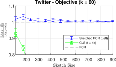
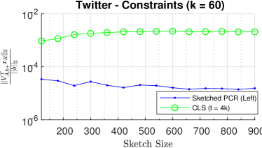
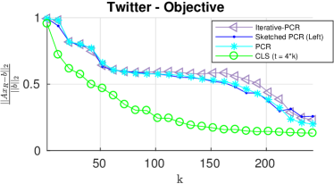
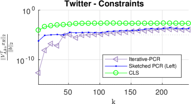
Figure 1: Sub-optimality of objective and constraint satisfaction for the Twitter Buzz dataset.

Generalization results.

We also explored the prediction error and the tradeoffs between compression and regularization. We perform each experiment five times and report the median value. Error bars, when present, represent the minimum and maximum value of those five runs.

We report the Mean Square Error (MSE) of predictions for the E2006.tfidf dataset in Figure 2. We compare CLS, iterative-PCR, right sketching and two-sided sketching (the matrix is too large for exact PCR, and $d\gg n$ so right sketching is more appropriate). In the left panel we fix $k=600$ and vary the sketch size. The MSE decreases as the sketch size increases for both sketching methods. For CLS, initially the MSE decreases and is close to the MSE of the two sketching methods, but for large sketch sizes the MSE starts to go up, likely due to decreased level of regularization. We note that the minimum MSE achieved by CLS is larger than achieved by both sketching methods. A similar phenomenon is observed when we vary the value of $k$ in the right panel.

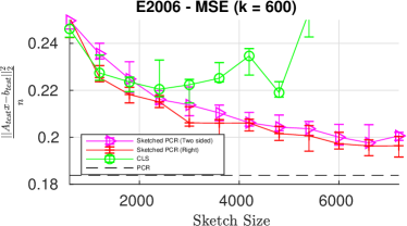
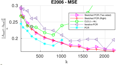
Figure 2: Mean squared error of predictions for the E2006.tfidf dataset.

We report the classification error for the Giesette dataset in Figure 3. In the left panel we fix $k=400$ and vary the sketch size. As a reference, the error rate of exact PCR (with $k=400$) is $2.8\%$ and the error rate for OLS is 9.3%. Left sketching has error rate very close to the error rate of exact PCR, especially when $s$ is large enough. Right sketching does not perform as well as left sketching, but it too achieves low error rate for large $s$. For both methods, the error rate drops as the sketch sizes increase, and the variance reduces. For CLS the error rate and variance initially drops as the sketch size increases, but eventually, when sketch size is large enough, the error rate and the variance increases. This is hardly surprising: as the sketch size increase, CLS approaches OLS. This is due to the fact that CLS uses the compression to regularize, and when the sketch size is large there is little regularization. In the right panel, we vary the value of $k$ and set $s=4k$ (left sketching) and $t=4k$ (right sketching and CLS). Left sketch and PCR consistently achieve about the same error rate. For small values of $t$, CLS performs well, but when $t$ is too large the error starts to increase. In contrast, right sketching continues to perform well with large values of $k$. Again, we see that CLS mixes compression and regularization, and one cannot use a large sketch size and modest amount of regularization with CLS.

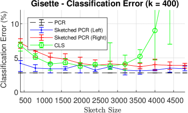
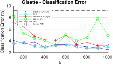
Figure 3: Classification error for the Gisette dataset.

Running time.

In Table 2 we report a sample of the various running times of the different algorithms. All experiments were conducted using MATLAB, although the sketching routines were written in C. Running times were measured on a machine with a 6-core Intel Xeon Processor E5-1650 v4 CPU and 128 GB of main memory, running Ubuntu 16.04. For plain PCR, we report running time using PRIMME, which we ran with default parameters and no preconditioner. For PRIMME, we cap the number of iterations at 100,000, and write “FAIL” in the table if the PRIMME failed to convergence within that cap. For iterative PCR we also report running times when we set tol to the default value, and reduce the max number of iteration from 40 to 10. This results in much faster running time, but much degraded generalization (not reported), e.g. for E2006 the test MSE for Iter-PCR (tol=$10^{-3}$, iter=10) is 0.32. With respect to running time, iterative-PCR is competitive with sketched PCR only for E2006, but with worse classification error. Using PRIMME for PCR is not competitive with sketched PCR. However, we stress that we experimented with only three datasets, so the comparison is not comprehensive.

Table 2: Running times (in seconds). For sketched PCR, we report in brackets the type of sketching used (left, right, or two-sided).

	CLS ($t=400)$	PRIMME-PCR	Iter-PCR (tol=$10^{-3}$, iter=10)	Iter-PCR (tol=$10^{-6}$)	Sketched-PCR
Twitter, $k=82$	21.2	1730	742	4067	4.7 (left)
Twitter, $k=152$	48.9	5907	1278	7759	8.4 (left)
E2006, $k=1000$	100	14694	140	601	150 (two sided)
E2006, $k=2000$	270	FAIL	320	791	815 (two sided)
Gisette, $k=400$	2.0	497	7.1	30.3	0.2 (left)
Gisette, $k=1000$	9.3	FAIL	9.3	39.4	0.9 (left)

7 Conclusions and Future work

In this paper, we studied the use of sketching to accelerate the solution of PCR and PCP. In particular, for a data matrix ${\bm{\mathrm{A}}}$, we relate the PCR/PCP solution of ${\bm{\mathrm{A}}}{\bm{\mathrm{R}}}$, where ${\bm{\mathrm{R}}}$ is any dimensionality reduction matrix, to the PCR/PCP solution of ${\bm{\mathrm{A}}}$. We presented a notion of approximate PCR/PCP, motivated both from an optimization perspective and from a statistical perspective, and provide conditions on ${\bm{\mathrm{R}}}$ that guarantee rigorous theoretical bounds. We then leverage the aforementioned results to design fast, sketching based, algorithms for approximate PCR/PCP, and demonstrate empirically the utility of our proposed algorithms. Throughout, our focus in this paper has been on algorithms that use the “sketch-and-solve” approach.

There are multiple ways in which the current work can be extended, and the theoretical results improved. We have presented two notions of approximation: approximate PCR and approximate PCP. Our results for approximate PCR use only dimensionality reduction matrices ${\bm{\mathrm{R}}}$ whose number of columns is equal to the target rank. It is natural to conjecture that the use of dimensionality reduction matrices with an higher number of columns will lead to stronger PCR bounds, but we prove only PCP bounds. The underlying reason is that our bounds for PCR are based on analyzing the distance between the column space of ${\bm{\mathrm{R}}}$ and the column space of ${\bm{\mathrm{V}}}_{{\bm{\mathrm{A}}},k}$ . However, once the number of columns in ${\bm{\mathrm{R}}}$ is different from the number of columns in ${\bm{\mathrm{V}}}_{{\bm{\mathrm{A}}},k}$, the definition of $d_{2}({\bm{\mathrm{R}}},{\bm{\mathrm{V}}}_{{\bm{\mathrm{A}}},k})$ is no longer applicable. One possible strategy for analyzing PCR when ${\bm{\mathrm{R}}}$ has more than $k$ columns might be to use a generalization of the distance between two subspaces that allows subspaces of different size; see [47] for such generalizations. Another crucial component will then be to generalize the Davis-Kahan theorem to bound such distances. We conjecture it is possible to derive algorithms that depend on gaps between $\sigma_{k}$ and $\sigma_{k+l}$, where $l$ is some oversampling parameter, as opposed to the smaller gap between $\sigma_{k}$ and $\sigma_{k+1}$. We leave this for future work.

Another interesting direction is in finding other ways to identify a valid approximate dominant subspace. If we consider the statistical perspective and inspect Eq. 9, we see that all we need is to find a subspace ${\cal S}\subseteq{\bf range}\left({\bm{\mathrm{A}}}\right)$ of rank $k$ such that $\|({\bm{\mathrm{I}}}-{\bm{\mathrm{P}}}_{{\cal S}}){\bm{\mathrm{A}}}\|_{F}$ is small, while our theoretical results try to achieve a stronger bound: having the dominant subspaces align. One possible way for finding such a ${\cal S}$ is using so-called Projection-cost Preserving Sketches [13]. We leave this for future work.

Acknowledgments.

This research was supported by the Israel Science Foundation (grant no. 1272/17) and by an IBM Faculty Award.

Appendix A Bias-Variance Decomposition for ${\cal E}({\mathbf{x}}_{{\bm{\mathrm{R}}}})$

The following appears, without proof, in [38]. For completeness, we include a proof.

Claim 20.

The excess risk of ${\mathbf{x}}_{{\bm{\mathrm{R}}}}$ can be bounded as follows:

$${\cal E}({\mathbf{x}}_{{\bm{\mathrm{R}}}})=\underset{{\cal B}({\mathbf{x}}_{{\bm{\mathrm{R}}}})}{\underbrace{\frac{1}{n}\|\left({\bm{\mathrm{I}}}-{\bm{\mathrm{P}}}_{{\bm{\mathrm{A}}}{\bm{\mathrm{R}}}}\right){\bm{\mathrm{A}}}{\mathbf{x}}^{\star}\|_{2}^{2}}}+\underset{{\cal V}({\mathbf{x}}_{{\bm{\mathrm{R}}}})}{\underbrace{\sigma^{2}\frac{{\bf rank}\left({\bm{\mathrm{A}}}{\bm{\mathrm{R}}}\right)}{n}}}\,.$$

Proof.

The column space of ${\bm{\mathrm{A}}}{\bm{\mathrm{R}}}$ is contained in the column space of ${\bm{\mathrm{A}}}$, so we have ${\bm{\mathrm{P}}}_{{\bm{\mathrm{A}}}{\bm{\mathrm{R}}}}={\bm{\mathrm{P}}}_{{\bm{\mathrm{A}}}{\bm{\mathrm{R}}}}{\bm{\mathrm{P}}}_{{\bm{\mathrm{A}}}}$. We now observe,

$${\cal E}({\mathbf{x}}_{{\bm{\mathrm{R}}}}) = \frac{1}{n}{\mathbb{E}}\left[\|{\bm{\mathrm{A}}}{\mathbf{x}}_{{\bm{\mathrm{R}}}}-{\bm{\mathrm{A}}}{\mathbf{x}}^{\star}\|_{2}^{2}\right]$$

$$= \frac{1}{n}{\mathbb{E}}\left[\|{\bm{\mathrm{P}}}_{{\bm{\mathrm{A}}}{\bm{\mathrm{R}}}}{\mathbf{b}}-{\bm{\mathrm{P}}}_{{\bm{\mathrm{A}}}}{\mathbf{f}}\|_{2}^{2}\right]$$

$$= \frac{1}{n}{\mathbb{E}}\left[\|{\bm{\mathrm{P}}}_{{\bm{\mathrm{A}}}{\bm{\mathrm{R}}}}{\mathbf{f}}-{\bm{\mathrm{P}}}_{{\bm{\mathrm{A}}}}{\mathbf{f}}\|_{2}^{2}\right]+\frac{1}{n}{\mathbb{E}}\left[\|{\bm{\mathrm{P}}}_{{\bm{\mathrm{A}}}{\bm{\mathrm{R}}}}\xi\|_{2}^{2}\right]$$

$$= \frac{1}{n}{\mathbb{E}}\left[\|{\bm{\mathrm{P}}}_{{\bm{\mathrm{A}}}{\bm{\mathrm{R}}}}{\bm{\mathrm{P}}}_{{\bm{\mathrm{A}}}}{\mathbf{f}}-{\bm{\mathrm{P}}}_{{\bm{\mathrm{A}}}}{\mathbf{f}}\|_{2}^{2}\right]+\sigma^{2}\frac{{\bf rank}\left({\bm{\mathrm{A}}}{\bm{\mathrm{R}}}\right)}{n}$$

$$= \frac{1}{n}\|\left({\bm{\mathrm{I}}}-{\bm{\mathrm{P}}}_{{\bm{\mathrm{A}}}{\bm{\mathrm{R}}}}\right){\bm{\mathrm{A}}}{\mathbf{x}}^{\star}\|_{2}^{2}+\sigma^{2}\frac{{\bf rank}\left({\bm{\mathrm{A}}}{\bm{\mathrm{R}}}\right)}{n}$$

where in the third line we used the fact that expected value of $\xi$ is $0$, and in the fourth line we used that fact that for any matrix ${\bm{\mathrm{M}}}$ and random vector ${\mathbf{y}}$ with independent entries with 0 mean and $\sigma^{2}$ variance we have ${\mathbb{E}}\left[{\mathbf{y}}^{\textsc{T}}{\bm{\mathrm{M}}}{\mathbf{y}}\right]={\bf Tr}\left({\bm{\mathrm{M}}}\right)$. ∎

References

• [1] Zeyuan Allen-Zhu and Yuanzhi Li. Faster principal component regression and stable matrix Chebyshev approximation. In Proceedings of the 34th International Conference on Machine Learning (ICML), 2017.
• [2] Andreas Artemiou and Bing Li. On principal components and regression: a statistical explanation of a natural phenomenon. Statistica Sinica, pages 1557–1565, 2009.
• [3] Haim Avron, Kenneth L. Clarkson, and David P. Woodruff. Faster kernel ridge regression using sketching and preconditioning. SIAM Journal on Matrix Analysis and Applications, 38(4):1116–1138, 2017.
• [4] Haim Avron, Kenneth L. Clarkson, and David P. Woodruff. Sharper Bounds for Regularized Data Fitting. In Klaus Jansen, José D. P. Rolim, David Williamson, and Santosh S. Vempala, editors, Approximation, Randomization, and Combinatorial Optimization. Algorithms and Techniques (APPROX/RANDOM 2017), volume 81 of Leibniz International Proceedings in Informatics (LIPIcs), pages 27:1–27:22, Dagstuhl, Germany, 2017. Schloss Dagstuhl–Leibniz-Zentrum fuer Informatik.
• [5] Haim Avron, Petar Maymounkov, and Sivan Toledo. Blendenpik: Supercharging LAPACK’s least-squares solver. SIAM Journal on Scientific Computing, 32(3):1217–1236, 2010.
• [6] Haim Avron, Huy Nguyen, and David Woodruff. Subspace embeddings for the polynomial kernel. In Neural Information Processing Systems (NIPS), 2014.
• [7] C. Boutsidis and M. Magdon-Ismail. Faster SVD-truncated regularized least-squares. In 2014 IEEE International Symposium on Information Theory, pages 1321–1325, June 2014.
• [8] Moses Charikar, Kevin Chen, and Martin Farach-Colton. Finding frequent items in data streams. Automata, Languages and Programming, pages 784–784, 2002.
• [9] Shouyuan Chen, Yang Liu, Michael R. Lyu, Irwin King, and Shengyu Zhang. Fast relative-error approximation algorithm for ridge regression. In Proceedings of the Thirty-First Conference on Uncertainty in Artificial Intelligence, UAI’15, pages 201–210, Arlington, Virginia, United States, 2015. AUAI Press.
• [10] Agniva Chowdhury, Jiasen Yang, and Petros Drineas. An iterative, sketching-based framework for ridge regression. In Jennifer Dy and Andreas Krause, editors, Proceedings of the 35th International Conference on Machine Learning, volume 80 of Proceedings of Machine Learning Research, pages 989–998, Stockholm, Sweden, 10–15 Jul 2018. PMLR.
• [11] Kenneth L. Clarkson and David P. Woodruff. Numerical linear algebra in the streaming model. In Proceedings of the Forty-first Annual ACM Symposium on Theory of Computing, STOC ’09, pages 205–214, New York, NY, USA, 2009. ACM.
• [12] Kenneth L. Clarkson and David P. Woodruff. Low-rank approximation and regression in input sparsity time. J. ACM, 63(6):54:1–54:45, January 2017.
• [13] Michael B. Cohen, Sam Elder, Cameron Musco, Christopher Musco, and Madalina Persu. Dimensionality reduction for k-means clustering and low rank approximation. In Rocco A. Servedio and Ronitt Rubinfeld, editors, Proceedings of the Forty-Seventh Annual ACM on Symposium on Theory of Computing, STOC 2015, Portland, OR, USA, June 14-17, 2015, pages 163–172. ACM, 2015.
• [14] Michael B. Cohen, Jelani Nelson, and David P. Woodruff. Optimal approximate matrix product in terms of stable rank. In 43rd International Colloquium on Automata, Languages, and Programming, ICALP 2016, July 11-15, 2016, Rome, Italy, pages 11:1–11:14, 2016.
• [15] Chandler Davis and William Morton Kahan. The rotation of eigenvectors by a perturbation. III. SIAM Journal on Numerical Analysis, 7(1):1–46, 1970.
• [16] Petros Drineas, Ilse Ipsen, Eugenia-Maria Kontopoulou, and Malik Magdon-Ismail. Structural convergence results for low-rank approximations from block Krylov spaces. CoRR, abs/1609.00671, 2016.
• [17] Petros Drineas, Michael W. Mahoney, S. Muthukrishnan, and Tamás Sarlós. Faster least squares approximation. Numerische Mathematik, 117(2):219–249, Feb 2011.
• [18] Roy Frostig, Cameron Musco, Christopher Musco, and Aaron Sidford. Principal component projection without principal component analysis. In International Conference on Machine Learning (ICML), pages 2349–2357, 2016.
• [19] Gene H. Golub and Charles F. Van Loan. Matrix Computations. JHU Press, 2012.
• [20] Alon Gonen, Francesco Orabona, and Shai Shalev-Shwartz. Solving ridge regression using sketched preconditioned SVRG. In Proceedings of the 33rd International Conference on International Conference on Machine Learning - Volume 48, ICML’16, pages 1397–1405. JMLR.org, 2016.
• [21] Nathan Halko, Per-Gunnar Martinsson, and Joel A Tropp. Finding structure with randomness: Probabilistic algorithms for constructing approximate matrix decompositions. SIAM Review, 53(2):217–288, 2011.
• [22] Roger A. Horn and Charles R. Johnson. Matrix Analysis. Cambridge University Press, 1990.
• [23] Harold Hotelling. Analysis of a complex of statistical variables into principal components. Journal of Educational Psychology, 24(6):417, 1933.
• [24] Ian T. Jolliffe. A note on the use of principal components in regression. Applied Statistics, pages 300–303, 1982.
• [25] Ata Kaban. New bounds on compressive linear least squares regression. In Samuel Kaski and Jukka Corander, editors, Proceedings of the Seventeenth International Conference on Artificial Intelligence and Statistics, volume 33 of Proceedings of Machine Learning Research, pages 448–456, Reykjavik, Iceland, 22–25 Apr 2014. PMLR.
• [26] Francois Kawala, Ahlame Douzal-Chouakria, Eric Gaussier, and Eustache Dimert. Prédictions d’activité dans les réseaux sociaux en ligne. In 4ième conférence sur les modèles et l’analyse des réseaux: Approches mathématiques et informatiques, 2013.
• [27] Maurice G. Kendall. A Course in Multivariate Analysis. C. Griffin, 1957.
• [28] Shimon Kogan, Dimitry Levin, Bryan R. Routledge, Jacob S. Sagi, and Noah A. Smith. Predicting risk from financial reports with regression. In Proceedings of Human Language Technologies: The 2009 Annual Conference of the North American Chapter of the Association for Computational Linguistics, pages 272–280. Association for Computational Linguistics, 2009.
• [29] Yichao Lu and Dean P. Foster. Fast ridge regression with randomized principal component analysis and gradient descent. In Uncertainty in Artificial Intelligence (UAI), 2014.
• [30] Odalric Maillard and Rémi Munos. Compressed least-squares regression. In Neural Information Processing Systems (NIPS), pages 1213–1221, 2009.
• [31] Xiangrui Meng, Michael A. Saunders, and Michael W. Mahoney. LSRN: A parallel iterative solver for strongly over- or underdetermined systems. SIAM Journal on Scientific Computing, 36(2):C95–C118, 2014.
• [32] Rasmus Pagh. Compressed matrix multiplication. ACM Trans. Comput. Theory, 5(3):9:1–9:17, 2013.
• [33] Ninh Pham and Rasmus Pagh. Fast and scalable polynomial kernels via explicit feature maps. In Proceedings of the 19th ACM SIGKDD International Conference on Knowledge Discovery and Data Mining, KDD ’13, pages 239–247, New York, NY, USA, 2013. ACM.
• [34] Mert Pilanci and Martin J. Wainwright. Randomized sketches of convex programs with sharp guarantees. IEEE Transactions on Information Theory, 61(9):5096–5115, 2015.
• [35] Mert Pilanci and Martin J. Wainwright. Iterative Hessian sketch: Fast and accurate solution approximation for constrained least-squares. The Journal of Machine Learning Research, 17(1):1842–1879, 2016.
• [36] Vladimir Rokhlin and Mark Tygert. A fast randomized algorithm for overdetermined linear least-squares regression. Proceedings of the National Academy of Sciences, 105(36):13212–13217, 2008.
• [37] Martin Slawski. Compressed least squares regression revisited. In Artificial Intelligence and Statistics (AISTATS), pages 1207–1215, 2017.
• [38] Martin Slawski. On Principal Components Regression, Random Projections, and Column Subsampling. ArXiv e-prints, September 2017.
• [39] Andreas Stathopoulos and James R. McCombs. PRIMME: PReconditioned Iterative MultiMethod Eigensolver: Methods and software description. ACM Transactions on Mathematical Software, 37(2):21:1–21:30, 2010.
• [40] Gilbert W. Stewart. On the perturbation of pseudo-inverses, projections and linear least squares problems. SIAM Review, 19(4):634–662, 1977.
• [41] Gilbert W Stewart. Matrix Algorithms: Volume II: Eigensystems. SIAM, 2001.
• [42] Gian-Andrea Thanei, Christina Heinze, and Nicolai Meinshausen. Random Projections for Large-Scale Regression, pages 51–68. Springer International Publishing, Cham, 2017.
• [43] Shusen Wang, Alex Gittens, and Michael W. Mahoney. Sketched ridge regression: Optimization perspective, statistical perspective, and model averaging. J. Mach. Learn. Res., 18(1):8039–8088, January 2017.
• [44] David P. Woodruff. Sketching as a tool for numerical linear algebra. Foundations and Trends® in Theoretical Computer Science, 10(1–2):1–157, 2014.
• [45] Lingfei Wu, Eloy Romero, and Andreas Stathopoulos. Primme_svds: A high-performance preconditioned SVD solver for accurate large-scale computations. SIAM Journal on Scientific Computing, 39(5):S248–S271, 2017.
• [46] Jiyan Yang, Xiangrui Meng, and Michael W. Mahoney. Implementing randomized matrix algorithms in parallel and distributed environments. Proceedings of the IEEE, 104(1):58–92, Jan 2016.
• [47] Ke Ye and Lek-Heng Lim. Schubert varieties and distances between subspaces of different dimensions. SIAM Journal on Matrix Analysis and Applications, 37(3):1176–1197, 2016.