Abstract

This paper demonstrates a mathematically correct and computationally powerful method for solving 3D topology optimization problems. This method is based on canonical duality theory (CDT) developed by Gao in nonconvex mechanics and global optimization. It shows that the so-called NP-hard knapsack problem in topology optimization can be solved deterministically in polynomial time via a canonical penalty-duality (CPD) method to obtain precise 0-1 global optimal solution at each volume evolution. The relation between this CPD method and Gao’s pure complementary energy principle is revealed for the first time. A CPD algorithm is proposed for 3-D topology optimization of linear elastic structures. Its novelty is demonstrated by benchmark problems. Results show that without using any artificial technique, the CPD method can provide mechanically sound optimal design, also it is much more powerful than the well-known BESO and SIMP methods. Additionally, computational complexity and conceptual/mathematical mistakes in topology optimization modeling and popular methods are explicitly addressed.

Keywords: Topology optimization, Bilevel Knapsack problem, Canonical Duality Theory (CDT), Canonical dual finite element method, Canonical Penalty-Duality method (CPD), Computational complexity.

1 Introduction

Topology optimization is a powerful tool for optimal design in multidisciplinary fields of optics, electronics, structural, bio and nano-mechanics. Mathematically speaking, this tool is based on finite element method such that the coupled variational problems in computational mechanics can be formulated as certain mixed integer nonlinear programming (MINLP) problems [19]. Due to the integer constraint, traditional theory and methods in continuous optimization can’t be applied for solving topology optimization problems. Therefore, most MINLP problems are considered to be NP-hard ($n$on-deterministic $p$olynomial-time hard) in global optimization and computer science [24]. During the past forty years, many approximate methods have been developed for solving topology optimization problems, these include homogenization method [4, 5], density-based method [3], Solid Isotropic Material with Penalization (SIMP) [42, 43, 54], level set approximation [39, 44], Evolutionary Structural Optimization (ESO) [51, 52] and bi-directional evolutionary structural optimization (BESO) [31, 40, 41]. Currently, the popular commercial software products used in topology optimization are based on SIMP and ESO/BESO methods [32, 37, 47, 53]. However, these approximate methods can’t mathematically guarantee the global convergence. Also, they usually suffer from having different intrinsic disadvantages, such as slow convergence, the gray scale elements and checkerboards patterns, etc [7, 45, 46].

Canonical duality theory (CDT) is a methodological theory, which was developed from Gao and Strang’s original work in 1989 on finite deformation mechanics [29]. The key feature of this theory is that by using certain canonical strain measure, general nonconvex/nonsmooth potential variational problems can be equivalently reformulated as a pure (stress-based only) complementary energy variational principle [12]. The associated triality theory provides extremality criteria for both global and local optimal solutions, which can be used to develop powerful algorithms for solving general nonconvex variational problems [13]. This pure complementary energy variational principle solved a well-known open problem in nonlinear elasticity and is known as the Gao principle in literature [36]. Based on this principle, a canonical dual finite element method was proposed in 1996 for large deformation nonconvex/nonsmooth mechanics [10]. Applications have been given to post-buckling problems of large deformed beams [2], nonconvex variational problems [25], and phase transitions in solids [30]. It was discovered by Gao in 2007 that by simply using a canonical measure $\epsilon(x)=x(x-1)=0$, the 0-1 integer constraint $x\in\{0,1\}$ in general nonconvex minimization problems can be equivalently converted to a unified concave maximization problem in continuous space, which can be solved deterministically to obtain global optimal solution in polynomial time [15]. Therefore, this pure complementary energy principle plays a fundamental role not only in computational nonlinear mechanics, but also in discrete optimization [26]. Most recently, Gao proved that the topology optimization should be formulated as a bi-level mixed integer nonlinear programming problem (BL-MINLP) [19, 21]. The upper-level optimization of this BL-MINLP is actually equivalent to the well-known Knapsack problem, which can be solved analytically by the CDT [21]. The review articles [16, 28] and the newly published book [24] provide comprehensive reviews and applications of the canonical duality theory in multidisciplinary fields of mathematical modeling, engineering mechanics, nonconvex analysis, global optimization, and computational science.

The main goal of this paper is to apply the canonical duality theory for solving 3-dimensional benchmark problems in topology optimization. In the next section, we first review Gao’s recent work why the topology optimization should be formulated as a bi-level mixed integer nonlinear programming problem. A basic mathematical mistake in topology optimization modeling is explicitly addressed. A canonical penalty-duality method for solving this Knapsack problem is presented in Section 3, which is actually the so-called $\beta$-perturbation method first proposed in global optimization [26] and recently in topology optimization [19]. Section 4 reveals for the first time the unified relation between this canonical penalty-duality method in integer programming and Gao’s pure complementary energy principle in nonlinear elasticity. Section 5 provides 3-D finite element analysis and the associated canonical penalty-duality (CPD) algorithm. The volume evolutionary method and computational complexity of this CPD algorithm are discussed. Applications to 3-D benchmark problems are provided in Section 6. The paper is ended by concluding remarks and open problems. Mathematical mistakes in the popular methods are explicitly addressed. Also, general modeling and conceptual mistakes in engineering optimization are discussed based on reviewers comments.

2 Mathematical Problems for 3-D Topology Optimization

The minimum total potential energy principle provides a theoretical foundation for all mathematical problems in computational solid mechanics. For general 3-D nonlinear elasticity, the total potential energy has the following standard form:

$$\Pi({\bf u},\rho)=\int_{\Omega}\bigg{(}W(\nabla{\bf u})\rho+{\bf u}\cdot{{\bf b}}\rho\bigg{)}d\Omega-\int_{\Gamma_{t}}{\bf u}\cdot{\bf t}d\Gamma,$$ (1)

where ${\bf u}:\Omega\rightarrow\mathbb{R}^{3}$ is a displacement vector field, ${{\bf b}}$ is a given body force vector, ${\bf t}$ is a given surface traction on the boundary $\Gamma_{t}\subset\partial\Omega$, the dot-product ${\bf u}\cdot{\bf t}={\bf u}^{T}{\bf t}$. In this paper, the stored energy density $W({\bf F})$ is an objective function (see Remark 4) of the deformation gradient ${\bf F}=\nabla{\bf u}$. In topology optimization, the mass density $\rho:\Omega\rightarrow\{0,1\}$ is the design variable, which takes $\rho({\bf x})=1$ at a solid material point ${\bf x}\in\Omega$, while $\rho({\bf x})=0$ at a void point ${\bf x}\in\Omega$. Additionally, it must satisfy the so-called knapsack condition:

$$\int_{\Omega}\rho({\bf x})d\Omega\leq V_{c},$$ (2)

where $V_{c}>0$ is a desired volume bound.

By using finite element method, the whole design domain $\Omega$ is meshed with $n$ disjointed finite elements $\{\Omega_{e}\}$. In each element, the unknown variables can be numerically written as ${\bf u}({\bf x})={\bf N}({\bf x}){\bf u}_{e},\;\;\rho({\bf x})=\rho_{e}\in\{0,1\}\;\;\forall{\bf x}\in\Omega_{e}$, where ${\bf N}({\bf x})$ is a given interpolation matrix, ${\bf u}_{e}$ is a nodal displacement vector. Let ${\cal U}_{a}\subset\mathbb{R}^{m}$ be a kinetically admissible space, in which certain deformation conditions are given, $v_{e}$ represents the volume of the $e$-th element $\Omega_{e}$, and ${\bf v}=\{v_{e}\}\in\mathbb{R}^{n}$. Then the admissible design space can be discretized as a discrete set

$${\cal Z}_{a}=\bigg{\{}\boldsymbol{\rho}=\{\rho_{e}\}\in\mathbb{R}^{n}\big{|}\;\;\rho_{e}\in\{0,1\}\;\forall e=1,\dots,n,\;\;\boldsymbol{\rho}^{T}{\bf v}=\sum_{e=1}^{n}\rho_{e}v_{e}\leq V_{c}\bigg{\}}$$ (3)

and on ${\cal U}_{a}\times{\cal Z}_{a},$ the total potential energy functional can be numerically reformulated as a real-valued function

$$\Pi_{h}({\bf u},\boldsymbol{\rho})=C(\boldsymbol{\rho},{\bf u})-{\bf u}^{T}{\bf f},$$ (4)

where

$$C(\boldsymbol{\rho},{\bf u})=\boldsymbol{\rho}^{T}{\bf c}({\bf u}),$$

in which

$${\bf c}({\bf u})=\bigg{\{}\int_{\Omega_{e}}[W(\nabla{\bf N}({\bf x}){\bf u}_{e})-{{\bf b}}^{T}{\bf N}({\bf x}){\bf u}_{e}]d\Omega\bigg{\}}\;\in\mathbb{R}^{n},$$ (5)

and

$${\bf f}=\bigg{\{}\int_{\Gamma_{t}^{e}}{\bf N}({\bf x})^{T}{\bf t}({\bf x})d\Gamma\bigg{\}}\in\mathbb{R}^{m}.$$

By the facts that the topology optimization is a combination of both variational analysis on a continuous space ${\cal U}_{a}$ and optimal design on a discrete space ${\cal Z}_{a}$, it can’t be simply formulated in a traditional variational form. Instead, a general problem of topology optimization should be proposed as a bi-level programming [21]:

$$({\cal{P}}_{bl}):\;\; \min\{\Phi(\boldsymbol{\rho},{\bf u})|\;\;{\boldsymbol{\rho}\in{\cal Z}_{a}},\;\;{\bf u}\in{\cal U}_{a}\},$$ (7)

$$\mbox{s.t.}\;\;{\bf u}\in\arg\min_{{\bf v}\in{\cal U}_{a}}\Pi_{h}({\bf v},\boldsymbol{\rho}),$$

where $\Phi(\boldsymbol{\rho},{\bf u})$ represents the upper-level cost function, $\boldsymbol{\rho}\in{\cal Z}_{a}$ is the upper-level variable. Simillarly, $\Pi_{h}({\bf u},\boldsymbol{\rho})$ represents the lower-level cost function and ${\bf u}\in{\cal U}_{a}$ is the lower-level variable. The cost function $\Phi(\boldsymbol{\rho},{\bf u})$ depends on both particular problems and numerical methods. It can be $\Phi(\boldsymbol{\rho}^{p},{\bf u})={\bf f}^{T}{\bf u}-{\bf c}({\bf u})^{T}\boldsymbol{\rho}^{p}$ for any given parameter $p\geq 1$, or simply $\Phi(\boldsymbol{\rho},{\bf u})=-\boldsymbol{\rho}^{T}{\bf c}({\bf u})$.

Since the topology optimization is a design-analysis process, it is reasonable to use the alternative iteration method [21] for solving the challenging topology optimization problem $({\cal{P}}_{bl})$, i.e.

(i) for a given design variable $\boldsymbol{\rho}_{k-1}\in{\cal Z}_{a}$, solving the lower-level optimization (7) for

$${\bf u}_{k}=\arg\min\{\Pi_{h}({\bf u},\boldsymbol{\rho}_{k-1})|\;\;{\bf u}\in{\cal U}_{a}\}$$ (8)

(ii) for the given ${\bf c}_{u}={\bf c}({\bf u}_{k})$, solve the upper-level optimization problem (7) for

$$\boldsymbol{\rho}_{k}=\arg\min\left\{\Phi(\boldsymbol{\rho},{\bf u}_{k})\;|\;\;\boldsymbol{\rho}\in{\cal Z}_{a}\right\}.$$ (9)

The upper-level problem (9) is actually equivalent to the well-known Knapsack problem in its most simple (linear) form:

$$({\cal{P}}_{u}):\;\;\min\{P_{u}(\boldsymbol{\rho})=-{\bf c}_{u}^{T}\boldsymbol{\rho}\;\;|\;\;\boldsymbol{\rho}^{T}{\bf v}\leq V_{c},\;\;\boldsymbol{\rho}\in\{0,1\}^{n}\},$$ (10)

which makes a perfect sense in topology optimization, i.e. among all elements $\{\Omega_{e}\}$, one should keep those stored more strain energy. Knapsack problems appear extensively in multidisciplinary fields of operations research, decision science, and engineering design problems. Due to the integer constraint, even this most simple linear knapsack problem is listed as one of Karp’s 21 NP-complete problems [34]. However, by using the canonical duality theory, this challenging problem can be solved easily to obtain global optimal solution.

For linear elastic structures without the body force, the stored energy $C$ is a quadratic function of ${\bf u}$:

$$C(\boldsymbol{\rho},{\bf u})=\frac{1}{2}{\bf u}^{T}{\bf K}(\boldsymbol{\rho}){\bf u},$$ (11)

where ${\bf K}(\boldsymbol{\rho})=\left\{\rho_{e}{\bf K}_{e}\right\}\in\mathbb{R}^{n\times n}$ is the overall stiffness matrix, obtained by assembling the sub-matrix $\rho_{e}{\bf K}_{e}$ for each element $\Omega_{e}$. For any given $\boldsymbol{\rho}\in{\cal Z}_{a}$, the displacement variable can be obtained analytically by solving the linear equilibrium equation ${\bf K}(\boldsymbol{\rho}){\bf u}={\bf f}$. Thus, the topology optimization for linear elastic structures can be simply formulated as

$$({\cal{P}}_{le}):\;\;\;\;\min\bigg{\{}{\bf f}^{T}{\bf u}-\frac{1}{2}{\bf u}^{T}{\bf K}(\boldsymbol{\rho}){\bf u}\;|\;\;{\bf K}(\boldsymbol{\rho}){\bf u}={\bf f},\;\;{\bf u}\in{\cal U}_{a},\;\;\boldsymbol{\rho}\in{{\cal Z}}_{a}\;\bigg{\}}.$$ (12)

Remark 1 (On Compliance Minimization Problem)

In literature, topology optimization for linear elastic structures is usually formulated as a compliance minimization problem (see [37] and the problem $(P)$ in [48]):

$$(P):\;\;\;\min_{\boldsymbol{\rho}\in\mathbb{R}^{n},{\bf u}\in{\cal U}_{a}}\;\;\frac{1}{2}{\bf f}^{T}{\bf u}\;\;s.t.\;\;{\bf K}(\boldsymbol{\rho}){\bf u}={\bf f},\;\;\boldsymbol{\rho}\in\{0,1\}^{n},\;\boldsymbol{\rho}^{T}{\bf v}\leq V_{c}.$$ (13)

Clearly, if the displacement is replaced by ${\bf u}=[{\bf K}(\boldsymbol{\rho})]^{-1}{\bf f}$, this problem can be written as

$$(P_{c}):\;\;\;\;\min\bigg{\{}P_{c}(\boldsymbol{\rho})=\frac{1}{2}{\bf f}^{T}[{\bf K}(\boldsymbol{\rho})]^{-1}{\bf f}\;|\;\;{\bf K}(\boldsymbol{\rho})\mbox{ {\rm is invertible for all }}\boldsymbol{\rho}\in{{\cal Z}}_{a}\;\bigg{\}}.$$ (14)

which is equivalent to $({\cal{P}}_{le})$ under the regularity condition, i.e. $[{\bf K}(\boldsymbol{\rho})]^{-1}$ exists for all $\boldsymbol{\rho}\in{\cal Z}_{a}$. However, instead of ${\bf u}$ the given external force in the cost function of $(P)$ is replaced by ${\bf f}={\bf K}{\bf u}$ such that $(P)$ is commonly written in the so-called minimization of strain energy (see [46]):

$$(P_{s}):\;\;\min\left\{\frac{1}{2}{\bf u}^{T}{\bf K}(\boldsymbol{\rho}){\bf u}\;|\;\;{\bf K}(\boldsymbol{\rho}){\bf u}={\bf f},\;\;\boldsymbol{\rho}\in{\cal Z}_{a},\;\;{\bf u}\in{\cal U}_{a}\;\;\right\},$$ (15)

One can see immediately that $(P_{s})$ contradicts $({\cal{P}}_{le})$ in the sense that the alternative iteration for solving $(P_{c})$ leads to an anti-Knapsack problem:

$$\min{\bf c}_{u}^{T}\boldsymbol{\rho},\;\;s.t.\;\;\boldsymbol{\rho}\in\{0,1\}^{n},\;\boldsymbol{\rho}^{T}{\bf v}\leq V_{c}.$$ (16)

By the fact that ${\bf c}_{u}={\bf c}({\bf u}_{k})\in\mathbb{R}^{n}_{+}:=\{{\bf c}\in\mathbb{R}^{n}|\;\;{\bf c}\geq{\bf 0}\}$ is a non-negative vector for any given ${\bf u}_{k}$, this problem has only a trivial solution. Therefore, the alternative iteration is not allowed for solving $({\cal{P}}_{s})$. In continuum physics, the linear scalar-valued function ${\bf u}^{T}{\bf f}\in\mathbb{R}$ is called the external (or input) energy, which is not an objective function (see Remark 4). Since ${\bf f}$ is a given force, it can’t be replaced by ${\bf K}(\boldsymbol{\rho}){\bf u}$. Although the cost function $P_{c}(\boldsymbol{\rho})$ can be called as the mean compliance, it is not an objective function either. Thus, the problem $(P_{c})$ works only for those problems that ${\bf u}(\boldsymbol{\rho})$ can be uniquely determined. Its complementary form

$$(P^{c}):\;\;\;\max\left\{\frac{1}{2}{\bf u}^{T}{\bf K}(\boldsymbol{\rho}){\bf u}\;\;|\;\;{\bf K}(\boldsymbol{\rho}){\bf u}={\bf f},\;\;\boldsymbol{\rho}\in{\cal Z}_{a}\right\}$$ (17)

can be called a maximum stiffness problem, which is equivalent to $({\cal{P}}_{le})$ in the sense that both problems produce the same results by the alternative iteration method. Therefore, it is a conceptual mistake to call the strain energy $\frac{1}{2}{\bf u}^{T}{\bf K}(\boldsymbol{\rho}){\bf u}$ as the mean compliance and $(P_{s})$ as the compliance minimization. The problem $(P_{s})$ has been used as a mathematical model for many approximation methods, including the SIMP and BESO. Additionally, some conceptual mistakes in the compliance minimization and mathematical modeling are also addressed in Remark 4.

3 Canonical Dual Solution to Knapsack Problem

The canonical duality theory for solving general integer programming problems was first proposed by Gao in 2007 [15]. Applications to topology optimization have been given recently in [19, 21]. In this paper, we present this theory in a different way, i.e. instead of the canonical measure in $\mathbb{R}^{n+1}$, we introduce a canonical measure in $\mathbb{R}^{n}$:

$$\boldsymbol{\varepsilon}={\Lambda}(\boldsymbol{\rho})=\boldsymbol{\rho}\circ\boldsymbol{\rho}-\boldsymbol{\rho}\in\mathbb{R}^{n}$$ (18)

and the associated super-potential

$$\Psi(\boldsymbol{\varepsilon})=\left\{\begin{array}[]{ll}0&\mbox{ if }\boldsymbol{\varepsilon}\in\mathbb{R}^{n}_{-}:=\{\boldsymbol{\varepsilon}\in\mathbb{R}^{n}|\;\;\boldsymbol{\varepsilon}\leq{\bf 0}\}\\ +\infty&\mbox{ otherwise},\end{array}\right.$$ (19)

such that the integer constraint in the Knapsack problem $({\cal{P}}_{u})$ can be relaxed by the following canonical form

$$\min\left\{\Pi_{u}(\boldsymbol{\rho})=\Psi({\Lambda}(\boldsymbol{\rho}))-{\bf c}_{u}^{T}\boldsymbol{\rho}\;\big{|}\;\;\boldsymbol{\rho}^{T}{\bf v}\leq V_{c}\;\;\boldsymbol{\rho}\in\mathbb{R}^{n}\right\}.$$ (20)

This is a nonsmooth minimization problem in $\mathbb{R}^{n}$ with only one linear inequality constraint. The classical Lagrangian for this inequality constrained problem is

$$L(\boldsymbol{\rho},\tau)=\Psi({\Lambda}(\boldsymbol{\rho}))-{\bf c}_{u}^{T}\boldsymbol{\rho}+\tau(\boldsymbol{\rho}^{T}{\bf v}-V_{c}),$$ (21)

and the canonical minimization problem (20) is equivalent to the following min-max problem:

$$\min_{\boldsymbol{\rho}\in\mathbb{R}^{n}}\max_{\tau\in\mathbb{R}}L(\boldsymbol{\rho},\tau)\;\;s.t.\;\;\tau\geq 0.$$ (22)

According to the Karush-Kuhn-Tucker theory in inequality constrained optimization, the Lagrange multiplier $\tau$ should satisfy the following KKT conditions:

$${\tau}(\boldsymbol{\rho}^{T}{\bf v}-V_{c})=0,\;\;{\tau}\geq 0,\;\;\boldsymbol{\rho}^{T}{\bf v}-V_{c}\leq 0.$$ (23)

The first equality ${\tau}(\boldsymbol{\rho}^{T}{\bf v}-V_{c})=0$ is the so-called complementarity condition. It is well-known that to solve the complementarity problems is not an easy task, even for linear complementarity problems [33]. Also, the Lagrange multiplier has to satisfy the constraint qualification ${\tau}\geq 0$. Therefore, the classical Lagrange multiplier theory can be essentially used for linear equality constrained optimization problems [35]. This is one of main reasons why the canonical duality theory was developed.

By the fact that the super-potential $\Psi(\boldsymbol{\varepsilon})$ is a convex, lower-semi continuous function (l.s.c), its sub-differential is a positive cone $\mathbb{R}^{n}_{+}$ [13]:

$$\partial\Psi(\boldsymbol{\varepsilon})=\left\{\begin{array}[]{ll}\{\mbox{\boldmath$\sigma$}\}\in\mathbb{R}^{n}_{+}&\;\mbox{ if }\boldsymbol{\varepsilon}\leq{\bf 0}\in\mathbb{R}^{n}_{-}\\ \;\;\emptyset&\mbox{ otherwise}.\end{array}\right.$$ (24)

Using Fenchel transformation, the conjugate function of $\Psi(\boldsymbol{\varepsilon})$ can be uniquely defined by (see [13])

$$\Psi^{\sharp}(\mbox{\boldmath$\sigma$})=\sup_{\boldsymbol{\varepsilon}\in\mathbb{R}^{n}}\{\boldsymbol{\varepsilon}^{T}\mbox{\boldmath$\sigma$}-\Psi(\boldsymbol{\varepsilon})\}=\left\{\begin{array}[]{ll}0&\mbox{ if }\mbox{\boldmath$\sigma$}\in\mathbb{R}^{n}_{+},\\ +\infty&\mbox{ otherwise},\end{array}\right.$$ (25)

which can be viewed as a super complementary energy [9]. By the theory of convex analysis, we have the following canonical duality relations [15]:

$$\Psi(\boldsymbol{\varepsilon})+\Psi^{\sharp}(\mbox{\boldmath$\sigma$})=\boldsymbol{\varepsilon}^{T}\mbox{\boldmath$\sigma$}\;\;\Leftrightarrow\;\;\mbox{\boldmath$\sigma$}\in\partial\Psi(\boldsymbol{\varepsilon})\;\;\Leftrightarrow\;\;\boldsymbol{\varepsilon}\in\partial\Psi^{\sharp}(\mbox{\boldmath$\sigma$}).$$ (26)

By the Fenchel-Young equality $\Psi(\boldsymbol{\varepsilon})=\boldsymbol{\varepsilon}^{T}\mbox{\boldmath$\sigma$}-\Psi^{\sharp}(\mbox{\boldmath$\sigma$})$, the Lagrangian $L(\boldsymbol{\rho},\tau)$ can be written in the following form

$$\Xi(\boldsymbol{\rho},\mbox{\boldmath$\sigma$},{\tau})=G_{ap}(\boldsymbol{\rho},\mbox{\boldmath$\sigma$})-\boldsymbol{\rho}^{T}\mbox{\boldmath$\sigma$}-\Psi^{\sharp}(\mbox{\boldmath$\sigma$})-\boldsymbol{\rho}^{T}{\bf c}_{u}+{\tau}(\boldsymbol{\rho}^{T}{\bf v}-V_{c}).$$ (27)

This is the Gao-Strang total complementary function for the Knapsack problem, in which, $G_{ap}(\boldsymbol{\rho},\mbox{\boldmath$\sigma$})=\mbox{\boldmath$\sigma$}^{T}(\boldsymbol{\rho}\circ\boldsymbol{\rho})$ is the so-called complementary gap function. Clearly, if $\mbox{\boldmath$\sigma$}\in\mathbb{R}^{n}_{+}$, this gap function is convex and $G_{ap}(\boldsymbol{\rho},\mbox{\boldmath$\sigma$})\geq 0\;\;\forall\boldsymbol{\rho}\in\mathbb{R}^{n}$. Let

$${\cal S}_{a}^{+}=\{\boldsymbol{\zeta}=\{\mbox{\boldmath$\sigma$},{\tau}\}\in\mathbb{R}^{n+1}|\;\;\mbox{\boldmath$\sigma$}>{\bf 0}\in\mathbb{R}^{n},\;\;{\tau}\geq 0\}.$$ (28)

Then on ${\cal S}_{a}$, we have

$$\Xi(\boldsymbol{\rho},\boldsymbol{\zeta})=\mbox{\boldmath$\sigma$}^{T}(\boldsymbol{\rho}\circ\boldsymbol{\rho}-\boldsymbol{\rho})-\boldsymbol{\rho}^{T}{\bf c}_{u}+{\tau}(\boldsymbol{\rho}^{T}{\bf v}-V_{c})$$ (29)

and for any given $\boldsymbol{\zeta}\in{\cal S}_{a}^{+}$, the canonical dual function can be obtained by

$$P^{d}_{u}(\boldsymbol{\zeta})=\min_{\boldsymbol{\rho}\in\mathbb{R}^{n}}\Xi(\boldsymbol{\rho},\boldsymbol{\zeta})=-\frac{1}{4}{\mbox{\boldmath$\tau$}}^{T}_{u}(\boldsymbol{\zeta}){\bf G}(\mbox{\boldmath$\sigma$})^{-1}{\mbox{\boldmath$\tau$}}_{u}(\boldsymbol{\zeta})-{\tau}V_{c},$$ (30)

where

$${\bf G}(\mbox{\boldmath$\sigma$})=\mathop{\rm Diag}(\mbox{\boldmath$\sigma$}),\;\;\;\;{\mbox{\boldmath$\tau$}}_{u}=\mbox{\boldmath$\sigma$}+{\bf c}_{u}-{\tau}{\bf v}.$$

This canonical dual function is the so-called pure complementary energy in nonlinear elasticity, first proposed by Gao in 1999 [12], where ${\mbox{\boldmath$\tau$}}_{u}$ and $\sigma$ are corresponding to the first and second Piola-Kirchhoff stresses, respectively. Thus, the canonical dual problem of the Knapsack problem can be proposed in the following

$$({\cal{P}}^{d}_{u}):\;\;\;\;\max\left\{P^{d}_{u}(\boldsymbol{\zeta})|\;\;\boldsymbol{\zeta}\in{\cal S}^{+}_{a}\right\}.$$ (31)

Theorem 1 (Canonical Dual Solution for Knapsack Problem [19])

For any given ${\bf u}_{k}\in{\cal U}_{a}$ and $V_{c}>0$, if $\bar{\boldsymbol{\zeta}}=(\bar{\mbox{\boldmath$\sigma$}},\bar{\tau})\in{\cal S}^{+}_{a}$ is a solution to $({\cal{P}}^{d}_{u})$, then

$$\bar{\boldsymbol{\rho}}=\frac{1}{2}{\bf G}(\bar{\mbox{\boldmath$\sigma$}})^{-1}{\mbox{\boldmath$\tau$}}_{u}(\bar{\boldsymbol{\zeta}})$$ (32)

is a global minimum solution to the Knapsack problem $({\cal{P}}_{u})$ and

$$P_{u}(\bar{\boldsymbol{\rho}})=\min_{\boldsymbol{\rho}\in\mathbb{R}^{n}}P_{u}(\boldsymbol{\rho})=\Xi(\bar{\boldsymbol{\rho}},\bar{\boldsymbol{\zeta}})=\max_{\boldsymbol{\zeta}\in{\cal S}^{+}_{a}}P^{d}_{u}(\boldsymbol{\zeta})=P_{u}^{d}(\bar{\boldsymbol{\zeta}}).$$ (33)

Proof. By the convexity of the super-potential $\Psi(\boldsymbol{\varepsilon})$, we have $\Psi^{**}(\boldsymbol{\varepsilon})=\Psi(\boldsymbol{\varepsilon})$. Thus,

$$L(\boldsymbol{\rho},\tau)=\sup_{\mbox{\boldmath$\sigma$}\in\mathbb{R}^{n}}\Xi(\boldsymbol{\rho},\mbox{\boldmath$\sigma$},\tau)\;\;\forall\boldsymbol{\rho}\in\mathbb{R}^{n},\;\;\tau\in\mathbb{R}.$$ (34)

It is easy to show that for any given $\boldsymbol{\rho}\in\mathbb{R}^{n},\;\tau\in\mathbb{R}$, the supremum condition is governed by ${\Lambda}(\boldsymbol{\rho})\in\partial\Psi^{*}(\mbox{\boldmath$\sigma$})$. By the canonical duality relations given in (26), we have the equivalent relations:

$${\Lambda}(\boldsymbol{\rho})^{T}\mbox{\boldmath$\sigma$}=\mbox{\boldmath$\sigma$}^{T}(\boldsymbol{\rho}\circ\boldsymbol{\rho}-\boldsymbol{\rho})=0\;\;\Leftrightarrow\;\;\mbox{\boldmath$\sigma$}\in\mathbb{R}^{n}_{+}\;\;\Leftrightarrow\;\;{\Lambda}(\boldsymbol{\rho})=(\boldsymbol{\rho}\circ\boldsymbol{\rho}-\boldsymbol{\rho})\in\mathbb{R}^{n}_{-}.$$ (35)

This is exactly equivalent to the KKT conditions of the canonical problem for the inequality condition ${\Lambda}(\boldsymbol{\rho})\in\mathbb{R}^{n}_{-}$. Thus, if $\bar{\boldsymbol{\zeta}}\in{\cal S}^{+}_{a}$ is a KKT solution to $({\cal{P}}^{d}_{u})$, then $\bar{\mbox{\boldmath$\sigma$}}>{\bf 0}$ and the complementarity condition in (35 ) leads to $\bar{\boldsymbol{\rho}}\circ\bar{\boldsymbol{\rho}}-\bar{\boldsymbol{\rho}}=0$, i.e. $\bar{\boldsymbol{\rho}}\in\{0,1\}^{n}$. It is easy to prove that for a given $\bar{\boldsymbol{\zeta}}$, the equality (32) is exactly the criticality condition $\nabla_{\boldsymbol{\rho}}\Xi(\bar{\boldsymbol{\rho}},\bar{\boldsymbol{\zeta}})=0$. Therefore, the vector $\bar{\boldsymbol{\rho}}\in\{0,1\}^{n}$ defined by (32) is a solution to the Knapsack problem $({\cal{P}}_{u})$. According to Gao and Strang [29] that the total complementary function $\Xi(\boldsymbol{\rho},\boldsymbol{\zeta})$ is a saddle function on $\mathbb{R}^{n}\times{\cal S}^{+}_{a}$, then

$$\min_{\boldsymbol{\rho}\in\mathbb{R}^{n}}P_{u}(\boldsymbol{\rho})=\min_{\boldsymbol{\rho}\in\mathbb{R}^{n}}\max_{\boldsymbol{\zeta}\in{\cal S}^{+}_{a}}\Xi(\boldsymbol{\rho},\boldsymbol{\zeta})=\max_{\boldsymbol{\zeta}\in{\cal S}^{+}_{a}}\min_{\boldsymbol{\rho}\in\mathbb{R}^{n}}\Xi(\boldsymbol{\rho},\boldsymbol{\zeta})=\max_{\boldsymbol{\zeta}\in{\cal S}^{+}_{a}}P^{d}_{u}(\boldsymbol{\zeta}).$$ (36)

The complementary-dual equality (33) can be proved by the canonical duality relations. $\Box$

This theorem shows that the so-called NP-hard Knapsack problem is canonically dual to a concave maximization problem $({\cal{P}}^{d}_{u})$ in continuous space, which is much easier than the 0-1 programming problem $({\cal{P}}_{u})$ in discrete space. Whence the canonical dual solution $\bar{\boldsymbol{\zeta}}$ is obtained, the solution to the Knapsack problem can be given analytically by (32).

4 Pure Complementary Energy Principle and Perturbed Solution

Based on Theorem 1, a perturbed solution for the Knapsack problem has been proposed recently in [19, 21]. This section demonstrates the relation of this solution with the pure complementary energy principle in nonlinear elasticity discovered by Gao in 1997-1999 [11, 12].

In terms of the deformation ${\mbox{\boldmath$\chi$}}={\bf u}+{\bf x}$, the total potential energy variational principle for general large deformation problems can also be written in the following form

$$({\cal{P}}_{\chi}):\;\;\;\inf_{{\mbox{\boldmath$\chi$}}\in{\cal X}_{a}}\Pi({\mbox{\boldmath$\chi$}})=\int_{\Omega}[W(\nabla{\mbox{\boldmath$\chi$}})-{\mbox{\boldmath$\chi$}}\cdot{{\bf b}}]\rho{\rm d}\Omega-\int_{\Gamma_{t}}{\mbox{\boldmath$\chi$}}\cdot{\bf t}{\rm d}\Gamma,$$ (37)

where ${\cal X}_{a}$ is a kinetically admissible deformation space, in which, the boundary condition ${\mbox{\boldmath$\chi$}}({\bf x})=0$ is given on $\Gamma_{\chi}$. It is well-known that the stored energy $W({\bf F})$ is usually a nonconvex function of the deformation gradient ${\bf F}=\nabla{\mbox{\boldmath$\chi$}}=\nabla{\bf u}+{\bf I}$ in order to model complicated phenomena, such as phase transitions and post-buckling. By the fact that $W({\bf F})$ must be an objective function [38], there exists a real-valued function $\Psi({\bf C})$ such that $W({\bf F})=\Psi({\bf F}^{T}{\bf F})$ (see [6]). For most reasonable materials (say the St. Venant-Kirchhoff material [23]), the function $\Psi({\bf C})$ is a usually convex function of the Cauchy strain measure ${\bf C}={\bf F}^{T}{\bf F}$ such that its complementary energy density can be uniquely defined by the Legendre transformation

$$\Psi^{*}({\bf S})=\{\;{\mbox{tr}}({\bf C}\cdot{\bf S})-\Psi({\bf C})|\;\;{\bf S}=\nabla\Psi({\bf C})\}.$$ (38)

Therefore, a pure complementary energy variational principle was obtained by Gao in 1999 [12, 13]:

Theorem 2 (Pure Complementary Energy Principle for Nonlinear Elasticity [12])

For any given external force field ${{\bf b}}({\bf x})$ in $\Omega$ and ${\bf t}({\bf x})$ on $\Gamma_{t}$, if $\tau({\bf x})$ is a statically admissible stress field, i.e.

$${\mbox{\boldmath$\tau$}}\in{\cal T}_{a}:=\left\{{\mbox{\boldmath$\tau$}}({\bf x}):\Omega\rightarrow\mathbb{R}^{3\times 3}|\;\;-\nabla\cdot{\mbox{\boldmath$\tau$}}={{\bf b}}\;\;\forall{\bf x}\in\Omega,\;\;{\bf n}\cdot{\mbox{\boldmath$\tau$}}={\bf t}\;\;\forall{\bf x}\in\Gamma_{t}\right\},$$ (39)

and $\bar{\bf S}$ is a critical point of the pure complementary energy

$$\Pi^{d}({\bf S})=-\int_{\Omega}\left[\frac{1}{4}{\mbox{tr}}({\mbox{\boldmath$\tau$}}\cdot{\bf S}^{-1}\cdot{\mbox{\boldmath$\tau$}})+\Psi^{*}({\bf S})\right]\rho\;{\rm d}\Omega,$$ (40)

then the deformation field ${\bar{{\mbox{\boldmath$\chi$}}}}({\bf x})$ defined by

$${\bar{{\mbox{\boldmath$\chi$}}}}({\bf x})=\frac{1}{2}\int_{{\bf x}_{0}}^{{\bf x}}{\mbox{\boldmath$\tau$}}\cdot\bar{\bf S}^{-1}d{\bf x}$$ (41)

along any path from ${\bf x}_{0}\in\Gamma_{\chi}$ to ${\bf x}\in\Omega$ is a critical point of the total potential energy $\Pi({\mbox{\boldmath$\chi$}})$ and $\Pi({\bar{{\mbox{\boldmath$\chi$}}}})=\Pi^{d}(\bar{\bf S})$. Moreover, if $\bar{\bf S}({\bf x})\succ 0\;\;\forall{\bf x}\in\Omega$, then ${\bar{{\mbox{\boldmath$\chi$}}}}$ is a global minimizer of $\Pi({\mbox{\boldmath$\chi$}})$.

It is easy to prove that the criticality condition $\delta\Pi^{d}_{\chi}({\bf S})=0$ is governed by the so-called canonical dual algebraic equation [13]:

$$4{\bf S}\cdot[\nabla\Psi^{*}({\bf S})]\cdot{\bf S}={\mbox{\boldmath$\tau$}}^{T}\cdot{\mbox{\boldmath$\tau$}}.$$ (42)

For certain materials, this algebraic equation can be solved analytically to obtain all possible solutions [25]. Particularly, for the St Venant-Kirchhoff material, this tensor equation could have at most 27 solutions at each material point ${\bf x}$, but only one positive-definite ${\bf S}({\bf x})\succ 0\;\;\forall{\bf x}\in\Omega$, which leads to the global minimum solution ${\bar{{\mbox{\boldmath$\chi$}}}}({\bf x})$ [23]. The pure complementary energy principle solved a well-known open problem in large deformation mechanics and is known as the Gao principle in literature (see [36]). This principle plays an important role not only in large deformation theory and nonconvex variational analysis, but also in global optimization and computational science. Indeed, Theorem 1 is simply an application of this principle as if we consider the quadratic operator $\boldsymbol{\varepsilon}(\boldsymbol{\rho})$ as the Cauchy strain measure ${\bf C}({\mbox{\boldmath$\chi$}})$, then the canonical dual $\mbox{\boldmath$\sigma$}\in\partial\Psi(\boldsymbol{\varepsilon})$ is corresponding to the second Piola-Kirchhoff stress ${\bf S}=\nabla\Psi({\bf C})$, while ${\mbox{\boldmath$\tau$}}_{u}$ is corresponding to the first Piola-Kirchhoff stress $\tau$. By the fact that $\Psi^{\sharp}(\mbox{\boldmath$\sigma$})$ is nonsmooth, the associated canonical dual algebraic equation (42) should be governed by the KKT conditions (35). In order to solve this problem, a $\beta$-perturbation method was proposed in 2010 for solving general integer programming problems [26] and recently for solving the topology optimization problems [19].

According to the canonical duality theory for mathematical modeling [21], the integer constraint $\boldsymbol{\rho}\in\{0,1\}^{n}$ in the Knapsack problem $({\cal{P}}_{u})$ is a constitutive condition, while $\boldsymbol{\rho}\cdot{\bf v}\leq V_{c}$ is a geometrical constraint. Thus, by using the so-called pan-penalty functions

$$W(\boldsymbol{\rho})=\left\{\begin{array}[]{ll}0&\mbox{ if }\boldsymbol{\rho}\in\{0,1\}^{n}\\ +\infty&\mbox{ otherwise},\end{array}\right.\;\;\;F(\boldsymbol{\rho})=\left\{\begin{array}[]{ll}{\bf c}_{u}\cdot\boldsymbol{\rho}&\mbox{ if }\boldsymbol{\rho}\cdot{\bf v}\leq V_{c}\\ -\infty&\mbox{ otherwise},\end{array}\right.$$ (43)

the Knapsack problem $({\cal{P}}_{u})$ can be equivalently written in Gao-Strang’s unconstrained form [29]:

$$\min\left\{W(\boldsymbol{\rho})-F(\boldsymbol{\rho})|\;\;\boldsymbol{\rho}\in\mathbb{R}^{n}\right\}.$$ (44)

By introducing a penalty parameter $\beta>0$ and a Lagrange multiplier $\tau\geq 0$, these two pan-penalty functions can have the following relaxations:

$$W_{\beta}(\boldsymbol{\rho})=\beta\|\boldsymbol{\rho}\circ\boldsymbol{\rho}-\boldsymbol{\rho}\|^{2},\;\;F_{\tau}(\boldsymbol{\rho})={\bf c}_{u}\cdot\boldsymbol{\rho}-\tau(\boldsymbol{\rho}\cdot{\bf v}-V_{c}).$$ (45)

It is easy to prove that

$$W(\boldsymbol{\rho})=\lim_{\beta\rightarrow\infty}W_{\beta}(\boldsymbol{\rho}),\;\;F(\boldsymbol{\rho})=\min_{\tau\geq 0}F_{\tau}(\boldsymbol{\rho})\;\;\forall\boldsymbol{\rho}\in\mathbb{R}^{n}.$$ (46)

Thus, the Knapsack problem can be relaxed by the so-called penalty-duality approach:

$$\min_{\boldsymbol{\rho}\in\mathbb{R}^{n}}\max_{\tau\geq 0}\left\{L_{\beta}(\boldsymbol{\rho},\tau)=W_{\beta}(\boldsymbol{\rho})-{\bf c}_{u}\cdot\boldsymbol{\rho}+\tau(\boldsymbol{\rho}\cdot{\bf v}-V_{c})\right\}.$$ (47)

Since the penalty function $W_{\beta}(\boldsymbol{\rho})$ is nonconvex, by using the canonical transformation $W_{\beta}(\boldsymbol{\rho})=\Psi_{\beta}({\Lambda}(\boldsymbol{\rho}))$, we have $\Psi_{\beta}(\boldsymbol{\varepsilon})=\beta\|\boldsymbol{\varepsilon}\|^{2}$, which is a convex quadratic function. Its Legendre conjugate is simply $\Psi^{*}_{\beta}(\mbox{\boldmath$\sigma$})=\frac{1}{4}\beta^{-1}\|\mbox{\boldmath$\sigma$}\|^{2}$. Thus, the Gao and Strang total complementary optimization problem for the penalty-duality approach (47) can be given by [19]:

$$\min_{\boldsymbol{\rho}\in\mathbb{R}^{n}}\max_{\boldsymbol{\zeta}\in{\cal S}^{+}_{a}}\left\{\Xi_{\beta}(\boldsymbol{\rho},\boldsymbol{\zeta})=(\boldsymbol{\rho}\circ\boldsymbol{\rho}-\boldsymbol{\rho})\cdot\mbox{\boldmath$\sigma$}-\frac{1}{4}\beta^{-1}\|\mbox{\boldmath$\sigma$}\|^{2}-{\bf c}_{u}\cdot\boldsymbol{\rho}+\tau(\boldsymbol{\rho}\cdot{\bf v}-V_{c})\right\}.$$ (48)

For any given $\beta>0$ and $\boldsymbol{\zeta}=\{\mbox{\boldmath$\sigma$},{\tau}\}\in{\bf S}^{+}_{a}$, a canonical penalty-duality (CPD) function can be obtained as

$$P^{d}_{\beta}(\boldsymbol{\zeta})=\min_{\boldsymbol{\rho}\in\mathbb{R}^{n}}\Xi_{\beta}(\boldsymbol{\rho},\boldsymbol{\zeta})=P^{d}_{u}(\mbox{\boldmath$\sigma$},{\tau})-\frac{1}{4}\beta^{-1}\|\mbox{\boldmath$\sigma$}\|^{2},$$ (49)

which is exactly the so-called $\beta$-perturbed canonical dual function presented in [19, 21]. It was proved by Theorem 7 in [26] that there exists a $\beta_{c}>0$ such that for any given $\beta\geq\beta_{c}$, both the CPD problem

$$({\cal{P}}^{d}_{\beta}):\;\;\;\max\{P^{d}_{\beta}(\boldsymbol{\zeta})|\;\;\boldsymbol{\zeta}\in{\cal S}^{+}_{a}\}$$ (50)

and the problem $({\cal{P}}^{d}_{u})$ have the same solution set. Since $\Psi_{\beta}^{*}(\mbox{\boldmath$\sigma$})$ is a quadratic function, the corresponding canonical dual algebraic equation (42) is a coupled cubic algebraic system

$$2\beta^{-1}{\sigma}_{e}^{3}+{\sigma}_{e}^{2}=(\tau v_{e}-c_{e})^{2},\;\;e=1,\dots,n,$$ (51)

$$\sum_{e=1}^{n}\frac{1}{2}\frac{v_{e}}{{\sigma}_{e}}({\sigma}_{e}-v_{e}\tau+c_{e})-V_{c}=0.$$ (52)

It was proved in [13, 15] that for any given $\beta>0$, $\tau\geq 0$ and ${\bf c}_{u}=\{c_{e}({\bf u}_{e})\}$ such that $\theta_{e}=\tau v_{e}-c_{e}({\bf u}_{e})\neq 0,\ e=1,\dots,n$, the canonical dual algebraic equation (51) has a unique positive real solution

$$\sigma_{e}=\frac{1}{12}\beta[-1+\phi_{e}(\tau)+\phi_{e}^{c}(\tau)]>0,\;\;e=1,\dots,n$$ (53)

where

$$\phi_{e}(\varsigma)=\eta^{-1/3}\left[2\theta_{e}^{2}-\eta+2i\sqrt{\theta_{e}^{2}(\eta-\theta_{e}^{2})}\right]^{1/3},\;\;\eta=\frac{\beta^{2}}{27},$$

and $\phi_{e}^{c}$ is the complex conjugate of $\phi_{e}$, i.e. $\phi_{e}\phi_{e}^{c}=1$. Thus, a canonical penalty-duality algorithm has been proposed recently for solving general topology optimization problems [19, 21].

5 CPD Algorithm for 3-D Topology Optimization

For three-dimensional linear elastic structures, we simply use cubic 8-node hexahedral elements $\{\Omega_{e}\}$, each element contains 24 degrees of freedom corresponding to the displacements in x-y-z directions (each node has three degrees of freedom) as shown in Fig. 1.

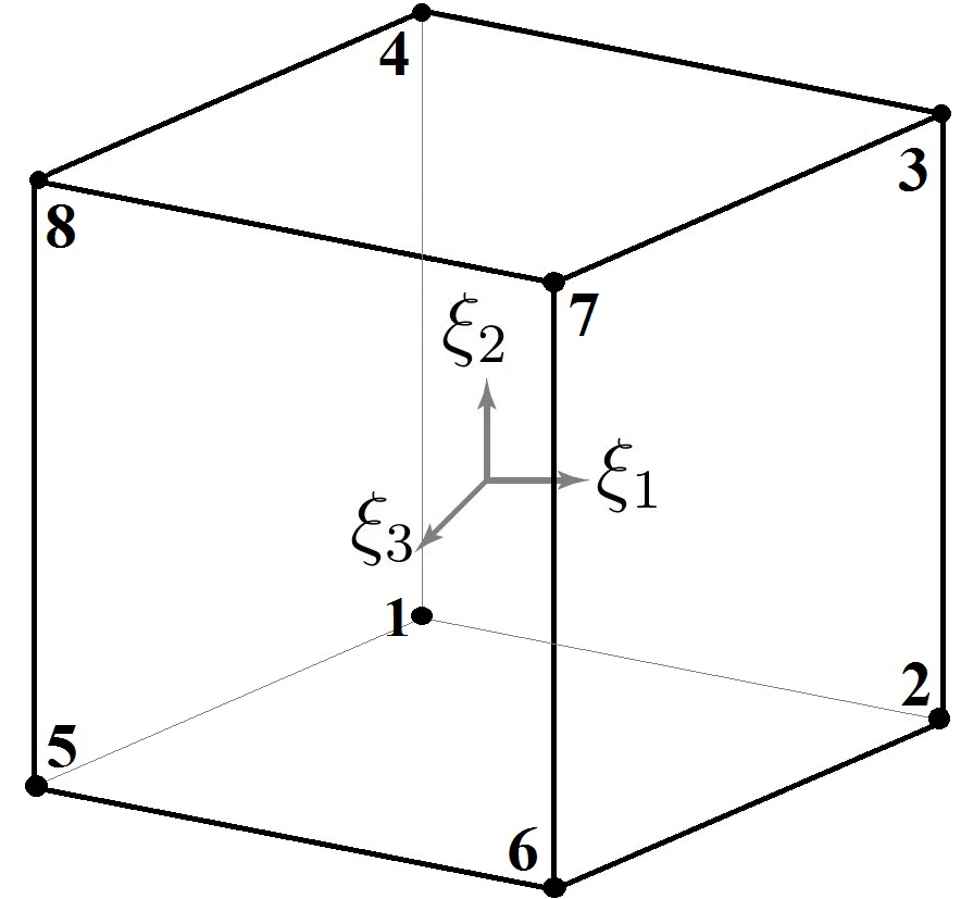
Figure 1: The hexahedron element - eight nodes

Thus, the displacement interpolation matrix is ${\bf N}=[\mathrm{N}_{1}\;\;\mathrm{N}_{2}\;\;...\;\;\mathrm{N}_{8}]$ and

$$\mathrm{N}_{i}=\left[\begin{array}[]{ccc}N_{i}&0&0\\ 0&N_{i}&0\\ 0&0&N_{i}\\ \end{array}\right].$$ (54)

The shape functions $N_{i}=N_{i}(\xi_{1},\xi_{2},\xi_{3})$, $i=1,...8$ are derived by

$$N_{1}=\frac{1}{8}(1-\xi_{1})(1-\xi_{2})(1-\xi_{3}),\;\;\;\;\;\;\;\;N_{2}=\frac{1}{8}(1+\xi_{1})(1-\xi_{2})(1-\xi_{3}),$$

$$N_{3}=\frac{1}{8}(1+\xi_{1})(1+\xi_{2})(1-\xi_{3}),\;\;\;\;\;\;\;\;N_{4}=\frac{1}{8}(1-\xi_{1})(1+\xi_{2})(1-\xi_{3}),$$

$$N_{5}=\frac{1}{8}(1-\xi_{1})(1-\xi_{2})(1+\xi_{3}),\;\;\;\;\;\;\;\;N_{6}=\frac{1}{8}(1+\xi_{1})(1-\xi_{2})(1+\xi_{3}),$$

$$N_{7}=\frac{1}{8}(1+\xi_{1})(1+\xi_{2})(1+\xi_{3}),\;\;\;\;\;\;\;\;N_{8}=\frac{1}{8}(1-\xi_{1})(1+\xi_{2})(1+\xi_{3}),$$

in which $\xi_{1},\xi_{2}$ and $\xi_{3}$ are the natural coordinates of the $i^{th}$ node. The nodal displacement vector ${\bf u}_{e}$ is given by

$${\bf u}_{e}^{T}=\left[u^{e}_{1}\;\;u^{e}_{2}\;\;...\;\;u^{e}_{8}\right],$$

where $u^{e}_{i}=(x^{e}_{i},y^{e}_{i},z^{e}_{i})\in\mathbb{R}^{3},\;i=1,...,8$ are the displacement components at node $i$. The components $\mathrm{B}_{i}$ of strain-displacement matrix ${\bf B}=[\mathrm{B}_{1}\;\mathrm{B}_{2}\;...\;\mathrm{B}_{8}]$, which relates the strain $\varepsilon$ and the nodal displacement ${\bf u}_{e}$ ($\varepsilon={\bf B}{\bf u}_{e}$), are defined as

$$\mathrm{B}_{i}=\left[\begin{array}[]{ccc}\frac{\partial N_{i}}{\partial x}&0&0\\ 0&\frac{\partial N_{i}}{\partial y}&0\\ 0&0&\frac{\partial N_{i}}{\partial z}\\ \frac{\partial N_{i}}{\partial y}&\frac{\partial N_{i}}{\partial x}&0\\ \frac{\partial N_{i}}{\partial z}&0&\frac{\partial N_{i}}{\partial x}\\ 0&\frac{\partial N_{i}}{\partial z}&\frac{\partial N_{i}}{\partial y}\\ \end{array}\right].$$ (55)

Hooke’s law for isotropic materials in constitutive matrix form is given by

$${\bf H}=\frac{E}{(1+\nu)(1-2\nu)}\left[\begin{array}[]{cccccc}1-\nu&\nu&\nu&0&0&0\\ \nu&1-\nu&\nu&0&0&0\\ \nu&\nu&1-\nu&0&0&0\\ 0&0&0&\frac{1-2\nu}{2}&0&0\\ 0&0&0&0&\frac{1-2\nu}{2}&0\\ 0&0&0&0&0&\frac{1-2\nu}{2}\end{array}\right],$$ (56)

where, $E$ is the Young’s modulus and $\nu$ is the Poisson’s ratio of the isotropic material. The stiffness matrix of the structure in CPD algorithm is given by

$${\bf K}(\boldsymbol{\rho})=\sum_{e=1}^{n}(E_{min}+(E-E_{min})\rho_{e})\mathrm{K}_{e},$$ (57)

where $E_{min}$ must be small enough (usually let $E_{min}=10-9E$) to avoid singularity in computation and $\mathrm{K}_{e}$ is defined as

$$\mathrm{K}_{e}=\int^{1}_{-1}\int^{1}_{-1}\int^{1}_{-1}{\bf B}^{T}{\bf H}{\bf B}\;d\xi_{1}d\xi_{2}d\xi_{3}.$$ (58)

Based on the canonical duality theory, an evolutionary canonical penalty-duality (CPD) algorithm for solving the topology optimization problem [19] can be presented in the following.
Canonical Penalty-Duality Algorithm for Topology Optimization (CPD):

1. Initialization:
   Choose a suitable initial volume reduction rate $\mu<1$.
   Let $\boldsymbol{\rho}^{0}=\{1\}\in\mathbb{R}^{n}$.
   Given an initial value ${\tau}^{0}>0$, an initial volume $V_{\gamma}=\mu V_{0}$.
   Given a perturbation parameter $\beta>10$, error allowances $\omega_{1}$ and $\omega_{2}$, in which $\omega_{1}$ is a termination criterion.
   Let $\gamma=0$ and compute

   $${\bf u}^{0}={\bf K}^{-1}(\boldsymbol{\rho}^{0}){\bf f}(\boldsymbol{\rho}^{0}),\;\;{\bf c}^{0}={\bf c}({\bf u}^{0})={{\bf u}^{0}}^{T}{\bf K}(\boldsymbol{\rho}^{0}){\bf u}^{0}.$$

2. Let $k=1$ .

3. Compute $\boldsymbol{\zeta}_{k}=\{\mbox{\boldmath$\sigma$}^{k},\tau^{k}\}$ by

   $$\sigma_{e}^{k}=\frac{1}{6}\beta[-1+\phi_{e}({\tau}^{k-1})+\phi_{e}^{c}({\tau}^{k-1})],\;\;e=1,\dots,n.$$

   $${\tau}^{k}=\frac{\sum_{e=1}^{n}v_{e}(1+c^{\gamma}_{e}/\sigma_{e}^{k})-2V_{\gamma}}{\sum_{e=1}^{n}v_{e}^{2}/\sigma_{e}^{k}}.$$

4. If

   $$\Delta=|P^{d}_{u}(\mbox{\boldmath$\sigma$}^{k},\tau^{k})-P^{d}_{u}(\mbox{\boldmath$\sigma$}^{k-1},\tau^{k-1})|>\omega_{1},$$ (59)

   then let $k=k+1$, go to Step 3; Otherwise, continue.

5. Compute $\boldsymbol{\rho}^{\gamma+1}=\{\rho^{\gamma+1}_{e}\}$ and ${\bf u}^{\gamma+1}$ by

   $$\rho^{\gamma+1}_{e}=\frac{1}{2}[1-({\tau}^{k}v_{e}-c^{\gamma}_{e})/\sigma_{e}^{k}],\;\;e=1,\dots,n.$$

   $${\bf u}^{\gamma+1}={\bf K}(\boldsymbol{\rho}^{\gamma+1})^{-1}{\bf f}(\boldsymbol{\rho}^{\gamma+1}).$$

6. If $|\boldsymbol{\rho}^{\gamma+1}-\boldsymbol{\rho}^{\gamma}|\leq\omega_{2}$ and $V_{\gamma}\leq V_{c}$ , then stop; Otherwise, continue.

7. Let $V_{\gamma+1}=\mu V_{\gamma}$, $\tau^{0}=\tau^{k}$, and $\gamma=\gamma+1$, go to step 2.

Remark 2 (Volume Evolutionary Method and Computational Complexity)

By Theorem 1 we know that for any given desired volume $V_{c}>0$, the optimal solution $\bar{\boldsymbol{\rho}}$ can be analytically obtained by (32) in terms of its canonical dual solution in continuous space. By the fact that the topology optimization problem $({\cal{P}}_{bl})$ is a coupled nonconvex minimization, numerical optimization depends sensitively on the the initial volume $V_{0}$. If $\mu_{c}=V_{c}/V_{0}\ll 1,$ any given iteration method could lead to unreasonable numerical solutions. In order to resolve this problem, a volume decreasing control parameter $\mu\in(\mu_{c},1)$ was introduced in [19] to produce a volume sequence $V_{\gamma}=\mu V_{\gamma-1}$ ($\gamma=1,\dots,\gamma_{c}$) such that $V_{\gamma_{c}}=V_{c}$ and for any given $V_{\gamma}\in[V_{c},V_{0}]$, the problem $({\cal{P}}_{bl})$ is replaced by

$$({\cal{P}}_{bl})^{\gamma}:\;\; \min \bigg{\{}{\bf f}^{T}{\bf u}-C_{p}(\boldsymbol{\rho},{\bf u})\;|\;\;\;\;\boldsymbol{\rho}\in\{0,1\}^{n},\;\;{\bf v}^{T}\boldsymbol{\rho}\leq V_{\gamma}\bigg{\}},$$ (60)

s.t. $${\bf u}(\boldsymbol{\rho})=\arg\min\{\Pi_{h}({\bf v},\boldsymbol{\rho})|\;\;{\bf v}\in{\cal U}_{a}\}.$$ (61)

The initial values for solving this $\gamma$-th problem are $V_{\gamma-1},{\bf u}_{\gamma-1},$ $\boldsymbol{\rho}_{\gamma-1}$. Theoretically speaking, for any given sequence $\{V_{\gamma}\}$ we should have

$$({\cal{P}}_{bl})=\lim_{\gamma\rightarrow\gamma_{c}}({\cal{P}}_{bl})^{\gamma}.$$ (62)

Numerically, different volume sequence $\{V_{\gamma}\}$ may produce totally different structural topology as long as the alternative iteration is used. This is intrinsic difficulty for all coupled bi-level optimal design problems.

The original idea of this sequential volume decreasing technique is from an evolutionary method for solving optimal shape design problems (see Chapter 7, [13]). It was realized recently that the same idea was used in the ESO and BESO methods. But these two methods are not polynomial-time algorithm. By the facts that there are only two loops in the CPD algorithm, i.e. the $\gamma$-loop and the $k$-loop, and the canonical dual solution is analytically given in the $k$-loop, the main computing is the $m\times m$ matrix inversion in the $\gamma$-loop. The complexity for the Gauss-Jordan elimination is $O(m^{3})$. Therefore, the CPD is a polynomial-time algorithm.

6 Applications to 3-D Benchmark Problems

In order to demonstrate the novelty of the CPD algorithm for solving 3D topology optimization problems, our numerical results are compared with the two popular methods: BESO and SIMP. The algorithm for the soft-kill BESO is from [32]. A modified SIMP algorithm without filter is used according to [37]. The parameters used in BESO and SIMP are: the minimum radius $r_{\min}=1.5$, the evolutionary rate $er=0.05$, and the penalization power $p=3$. Young’s modulus and Poisson’s ratio of the material are taken as $E=1$ and $\nu=0.3$, respectively. The initial value for ${\tau}$ used in CPD is ${\tau}^{0}=1$. We take the design domain $V_{0}=1$, the initial design variable $\boldsymbol{\rho}^{0}=\{1\}$ for both CPD and BESO algorithms. All computations are performed by a computer with Processor Intel Core I7-4790, CPU 3.60GHz and memory 16.0 GB.

6.1 Cantilever Beam Problems

For this benchmark problem, we present results based on three types of mesh resolutions with two types of loading conditions.

6.1.1 Uniformly distributed load with $60\times 20\times 4$ meshes.

First, let us consider the cantilever beam with uniformly distributed load at the right end as illustrated in Fig. 2.

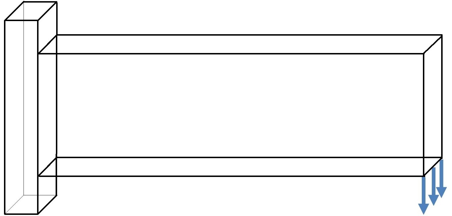
Figure 2: Cantilever beam with uniformly distributed load in the right end

The target volume and termination criterion for CPD, BESO and SIMP are selected as $V_{c}=0.3$ and $\omega_{1}=10^{-6}$, respectively. For both CPD and BESO methods, we take the volume evolution rate $\mu=0.89$, the perturbation parameter for CPD is $\beta=4000$. The results are reported in Table 1.

Method	Details	Structure
CPD	$C=1973.028$ It. = 23 Time= 27.1204
BESO	$C=1771.3694$ It. = 154 Time= 2392.9594
SIMP	$C=2416.6333$ It. = 200 Time= 98.7545

Table 1: Structures produced by CPD, BESO and SIMP for cantilever beam ($60\times 20\times 4$)

Fig. 3 shows the convergence of compliances produced by all the three methods. As we can see that the SIMP provides an upper bound approach since this method is based on the minimization of the compliance, i.e. the problem $(P)$. By Remark 1 we know that this problem violates the minimum total potential energy principle, the SIMP converges in a strange way, i.e. the structures produced by the SIMP at the beginning are broken until $It.=15$ (see Fig. 3), which is physically unreasonable. Dually, both the CPD and BESO provide lower bound approaches. It is reasonable to believe that the main idea of the BESO is similar to the Knapsack problem, i.e. at each volume iteration, to eliminate elements which stored less strain energy by simply using comparison method. By the fact that the same volume evolutionary rate $\mu$ is adopted, the results obtained by the CPD and BESO are very close to each other (see also Fig. 4). However, the CPD is almost 100 times faster than the BESO method since the BESO is not a polynomial-time algorithm.

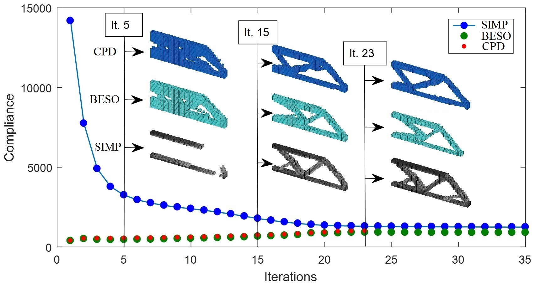
Figure 3: Convergence test for CPD, BESO and SIMP

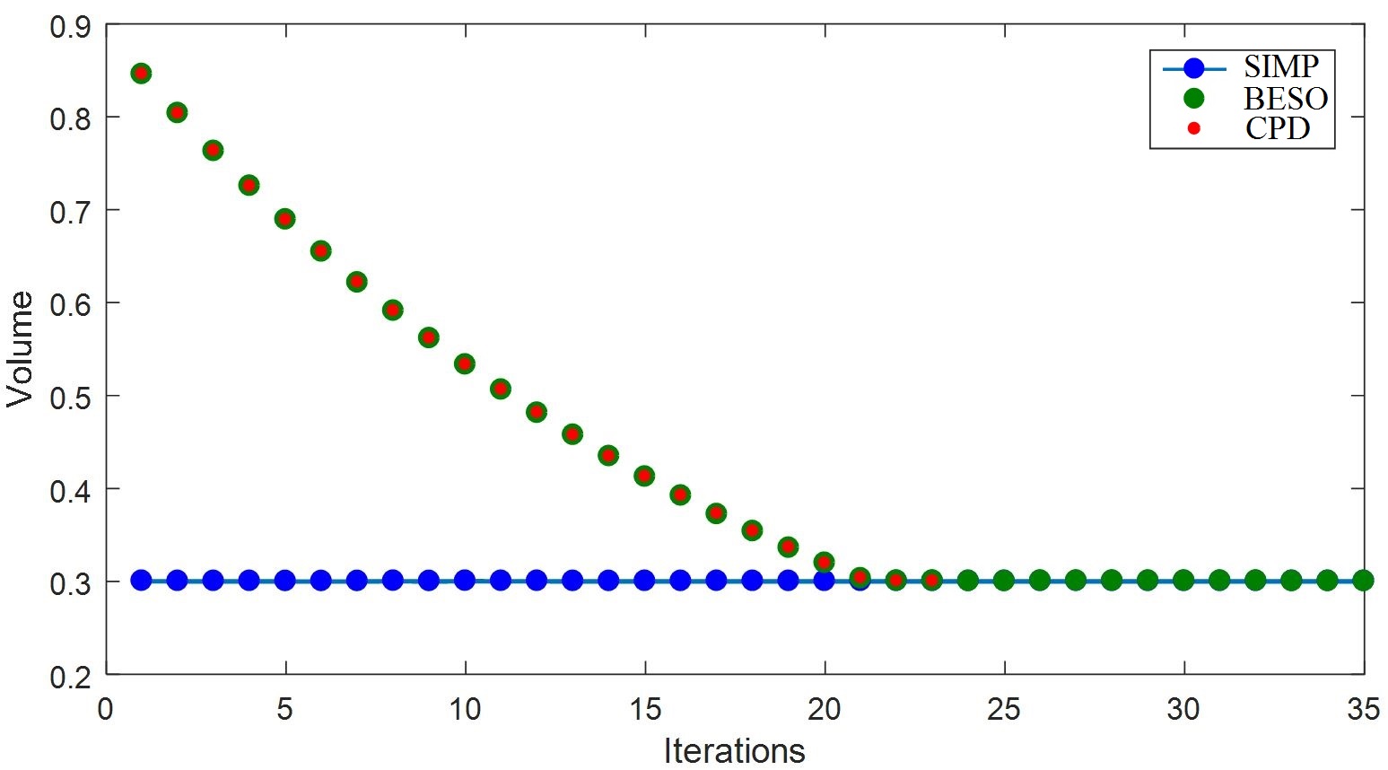
Figure 4: Comparison of volume variations for CPD, BESO and SIMP

The optimal structures produced by the CPD with $\omega_{1}=10^{-16}$ and with different values of $\mu$ and $\beta$ are summarized in Table 2. Also, the target compliances during the iterations for all CPD examples are reported in Figs. 5 with different values of $\mu$ and $\beta$. The results show that the CPD algorithm is sensitively depends on the volume evolution parameter $\mu$, but not the penalty parameter $\beta$. The comparison for volume evolutions by CPD and BESO is given in Fig 6, which shows as expected that the BESO method also sensitively depends on the volume evolutionary rate $\mu$. For a fixed $\beta=4000$, the convergence of the CPD is more stable and faster than the BESO. The $C$-Iteration curve for BESO jumps for every given $\mu$, which could be the so-called “chaotic convergence curves” addressed by G. I. N. Rozvany in [42].

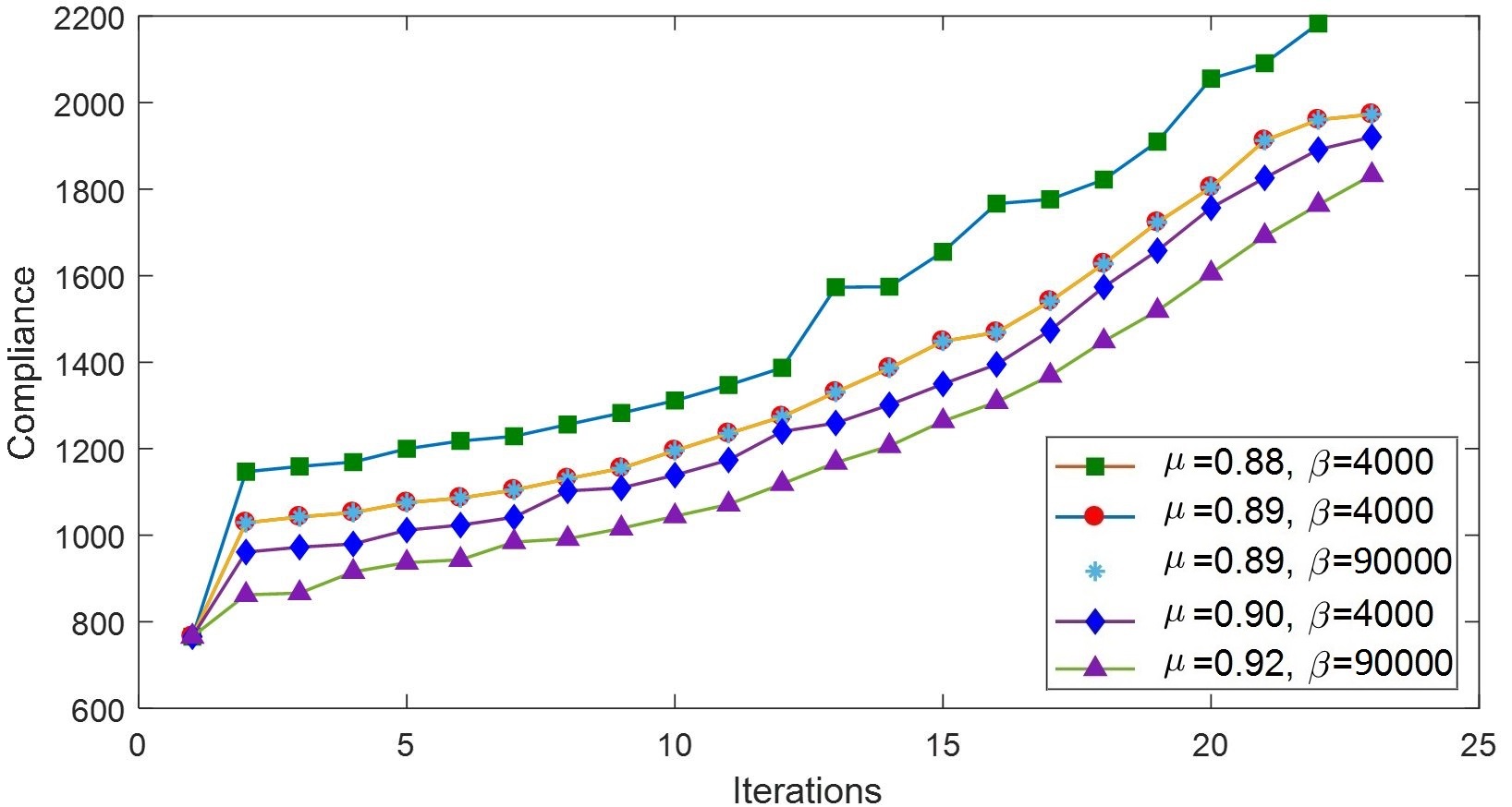
Figure 5: Convergence tests for CPD method at different values of $\mu$ and $\beta$

Figure 6: Convergence test for CPD and BESO with different $\mu$.

Details	Structure	Details	Structure
$\mu=0.88$ $\beta=4000$ $C=2182.78$ It. =22 Time=29.44		$\mu=0.89$ $\beta=90000$ $C=1973.02$ It. =23 Time=30.69
$\mu=0.9$ $\beta=4000$ $C=1920.68$ It. =23 Time=30.87		$\mu=0.92$ $\beta=90000$ $C=1832.59$ It. =23 Time=33.73

Table 2: Optimal structures produced by CPD with different values of $\mu$ and $\beta$

6.1.2 Uniformly distributed load with $120\times 50\times 8$ mesh resolution

Now let us consider the same loaded beam as shown in Fig 2 but with a finer mesh resolution of $120\times 50\times 8$. In this example the target volume fraction and termination criterion for all procedures are assumed to be $V_{c}=0.3$ and $\omega_{1}=10^{-6}$, respectively. The initial volume reduction rate for both CPD and BESO is $\mu=0.935$. The perturbation parameter for CPD is $\beta=7000$. The optimal topologies produced by CPD, BESO and SIMP methods are reported in Table 3. As we can see that the CPD is about five times faster than the SIMP and almost 100 times faster than the BESO method.

If we choose $\omega_{1}=0.001$, the computing times (iterations) for CPD, BESO and SIMP are 0.97 (24), 24.67 (44) and 4.3 (1000) hours, respectively. Actually, the SIMP failed to reach the given precision. If we increase $\omega_{1}=0.01$, the SIMP takes 3.14 hours with 742 iterations to satisfy the given precision. Our numerical results show that the CPD method can produce very good results with much less computing time. For a given very small $\omega_{1}=10^{-16}$, Table 4 shows the effects of the parameters of $\mu,\;\beta$ and $V_{c}$ on the computing time of the CPD method.

Method	Details	Structure
CPD	$C=1644.0886$ It. =24 Time=3611.23
BESO	$C=1605.1102$ It. =200 Time=342751.96
SIMP	$C=1835.4106$ It. =1000 Time=15041.06

Table 3: Topology optimization for cantilever beam ($120\times 50\times 8$)

$\;\mu=0.935,\;\;\beta=3000,\;V_{c}=0.3$ $C=1632.959$, It. =25, Time=3022.029	$\;\mu=0.935,\;\;\beta=7000,\;V_{c}=0.18$ $C=2669.980$, It. =34, Time=5040.6647
$\;\mu=0.98,\;\;\beta=7000,\;V_{c}=0.3$ $C=1635.922$, It. =25, Time=3531.3235	$\;\mu=0.98,\;\;\beta=7000,\;V_{c}=0.18$ $C=2892.914$, It. =35, Time=4853.3776

Table 4: Effects of $\mu$, $\beta$ and $V_{c}$ to the final results by CPD method ($\omega_{1}=10^{-16}$)

6.1.3 Beam with a central load and $40\times 20\times 20$ meshes

In this example, the beam is subjected to a central load at its right end (see Fig. 7). We let $V_{c}=0.095$, $\omega_{1}=0.001$, $\beta=7000$ and $\mu=0.888$.

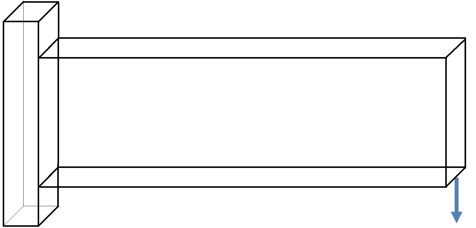
Figure 7: Design domain for cantilever beam with a central load in the right end

The topology optimized structures produced by CPD, SIMP and BESO methods are summarized in Table 5. Compared with the SIMP method, we can see that by using only $20\%$ of computing time, the CPD can produce global optimal solution, which is better than that produced by the BESO, but with only $8\%$ of computing time. We should point out that for the given $\omega_{1}=0.001$, the SIMP method failed to converge in 1000 iterations (the so-called “change” $\Delta=0.0061>\omega_{1}$).

CPD:   $C=20.564,$    It. =45,  Time=959.7215
BESO:   $C=20.1533,$   It. =53,  Time=11461.128
SIMP:   $C=25.7285,$   It. =1000,  Time=4788.4762

Table 5: Topologies of the cantilever beam with a central load in the right end

6.2 MBB Beam

The second benchmark problem is the 3-D Messerschmitt-$\mathrm{\ddot{B}olkow}$-Blohm (MBB) beam. Two examples with different loading and boundary conditions are illustrated.

6.2.1 Example 1

The MBB beam design for this example is illustrated in Fig. 8. In this example, we use $40\times 20\times 20$ mesh resolution, $V_{c}=0.1$ and $\omega_{1}=0.001$. The initial volume reduction rate and perturbation parameter are $\mu=0.89$ and $\beta=5000$, respectively.

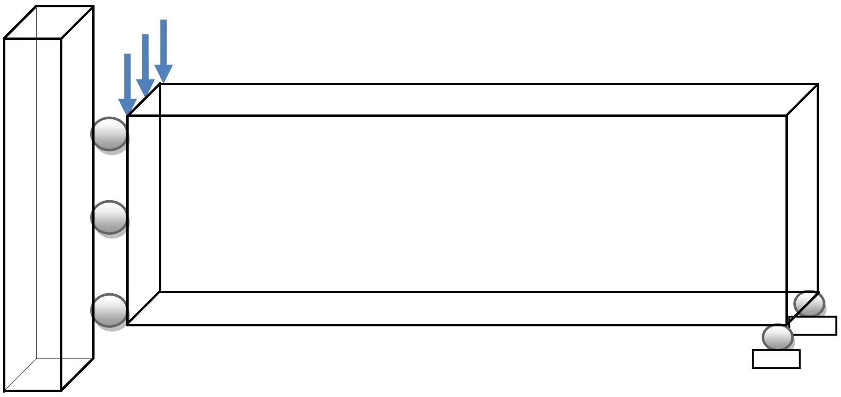
Figure 8: MBB beam with uniformly distributed central load

Table 6 summarizes the optimal topologies by using CPD, BESO and SIMP methods. Compared with the BESO method, we see again that the CPD produces a mechanically sound structure and takes only $12.6\%$ of computing time. Also, the SIMP method failed to converge for this example and the result presented in Table 6 is only the output of the 1000th iteration when $\Delta=0.039>\omega_{1}$.

CPD:   $C=7662.5989,$    It. =46,  Time=1249.1267
BESO:   $C=7745.955,$   It. =55,  Time=9899.0921
SIMP:   $C=12434.8629,$   It. =1000,  Time=5801.0065

Table 6: Results for 3-D MBB beam with uniformly distributed load

6.2.2 Example 2

In this example, the MBB beam is supported horizontally in its four bottom corners under central load as shown in Fig. 9.

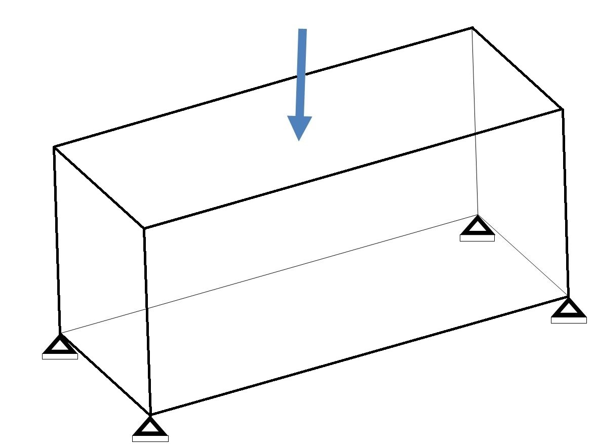
Figure 9: 3-D MBB beam with a central load

The mesh resolution is $60\times 10\times 10$, the target volume is $V_{c}=0.155$. The initial volume reduction rate and perturbation parameter are defined as $\mu=0.943$ and $\beta=7250$, respectively.

The topology optimized structures produced by CPD, BESO and SIMP with $\omega_{1}=10^{-5}$ are reported in Table 7. Once again we can see that without using any artificial techniques, the CPD produces mechanically sound integer density distribution but the computing time is only 3.3% of that used by the BESO.

Method	Details	Structure
CPD	$C=19.5313\;\;\;$ It. = 37 Time=48.2646
BESO	$C=20.1132\;\;\;$ It. =57 Time=1458.488
SIMP	$C=41.4099\;\;\;$ It. =95 Time=366.4988

Table 7: Structures for 3-D MBB beam with a central load

6.3 Cantilever beam with a given hole

In real-world applications, the desired structures are usually subjected to certain design constraints such that some elements are required to be either solid or void. Now let us consider the cantilever beam with a given hole as illustrated in Fig. 10. We use mesh resolution $70\times 30\times 6$ and parameters $V_{c}=0.5$, $\beta=7000$, $\mu=0.94$ and $\omega_{1}=0.001$.

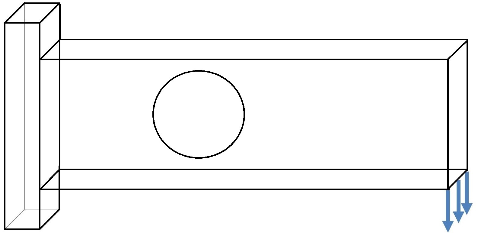
Figure 10: Design domain for cantilever beam with a given hole

The optimal topologies produced by CPD, BESO, and SIMP are summarized in Table 8. The results show clearly that the CPD method is significantly faster than both BESO and SIMP. Again, the SIMP failed to converge in 1000 iterations and the “Change” $\Delta=0.011>\omega_{1}$ at the last iteration.

CPD:   $C=910.0918,$    It. =14,  Time=74.61
BESO:   $C=916.3248,$   It. =21,  Time=1669.5059
SIMP:   $C=997.1556,$   It. =1000,  Time=1932.7697

Table 8: Topology optimized structures for cantilever beam with a given hole

6.4 3D wheel problem

The 3D wheel design problem is constrained by planar joint on the corners with a downward point load in the center of the bottom as shown in Fig. 11. The mesh resolution for this problem is $40\times 20\times 40$. The target volume is $V_{c}=0.2$ and the parameters used are $\beta=150$, $\mu=0.94$ and $\omega_{1}=10^{-5}$. The optimal topologies produced by CPD, BESO and SIMP are reported in Table 9. We can see that the CPD takes only about 18% and 32% of computing times by BESO and SIMP, respectively. Once again, the SIMP failed to converge in 1000 iterations and the “Change” $\Delta=0.0006>\omega_{1}$ at the last iteration.

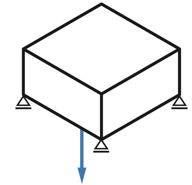
Figure 11: 3D wheel problem

$C=3.6164$, It. =32 Time=6716.1433	$C=3.6136$, It. =52 Time=37417.5089	$C=3.7943$, It. =1000 Time=20574.8348

Table 9: Topology optimized results for 3D-wheel problem ($40\times 20\times 40$) by CPD (left), BESO (middle), and SIMP (right)

$\mu=0.88,\;\;V_{c}=0.06$ $C=5.7296$, It. =55 Time=2324.0445	$\mu=0.88,\;\;V_{c}=0.1$ $C=4.2936$, It. =44 Time=1888.6451	$\mu=0.92,\;\;V_{c}=0.1$ $C=4.3048$, It. =45 Time=1823.7826

Table 10: Topology optimized results by CPD for 3D-wheel problem ($30\times 20\times 30$) with two different views

For a given very small termination criterion $\omega_{1}=10^{-16}$ and for mesh resolution $30\times 20\times 30$, Table 10 shows effects of the parameters $\mu$ and $V_{c}$ on the topology optimized results by CPD.

7 Concluding Remarks and Open Problems

We have presented a novel canonical penalty-duality method for solving challenging topology optimization problems. The relation between the CPD method for solving 0-1 integer programming problems and the pure complementary energy principle in nonlinear elasticity is revealed for the first time. Applications are demonstrated by 3-D linear elastic structural topology optimization problems. By the fact that the integer density distribution is obtained analytically, it should be consider as the global optimal solution at each volume iteration. Generally speaking, the so-called compliance produced by the CPD is higher than those by BESO for most of tested problems except for the MBB beam and the cantilever beam with a given hole. The possible reason is that certain artificial techniques such as the so-called soft-kill, filter and sensitivity are used by the BESO method. The following remarks are important for understanding these popular methods and conceptual mistakes in topology optimization.

Remark 3 (On Penalty-Duality, SIMP, and BESO Methods)

It is well-known that the Lagrange multiplier method can be used essentially for solving convex problem with equality constraints. The Lagrange multiplier must be a solution to the Lagrangian dual problem (see the Lagrange Multiplier’s Law in [13], page 36). For inequality constraint, the Lagrange multiplier must satisfy the KKT conditions. The penalty method can be used for solving problems with both equality and inequality constraints, but the iteration method must be used. By the facts that the penalty parameter is hard to control during the iterations and in principle, needs to be large enough for the penalty function to be truly effective, which on the other hand, may cause numerical instabilities, the penalty method was becoming disreputable after the augmented Lagrange multiplier method was proposed in 1970 and 1980s. The augmented Lagrange multiplier method is simply the combination of the Lagrange multiplier method and the penalty method, which has been actively studied for more than 40 years. But this method can be used mainly for solving linearly constrained problems since any simple nonlinear constraint could lead to a nonconvex minimization problem [35].

For example, let us consider the knapsack problem $({\cal{P}}_{u})$. As we know that by using the canonical measure ${\Lambda}(\boldsymbol{\rho})=\boldsymbol{\rho}\circ\boldsymbol{\rho}-\boldsymbol{\rho}$, the 0-1 integer constraint $\boldsymbol{\rho}\in\{0,1\}^{n}$ can be equivalently written in equality $\boldsymbol{\rho}\circ\boldsymbol{\rho}-\boldsymbol{\rho}={\bf 0}$. Even for this most simple quadratic nonlinear equality constraint, its penalty function $W_{\beta}=\beta\|\boldsymbol{\rho}\circ\boldsymbol{\rho}-\boldsymbol{\rho}\|^{2}$ is a nonconvex function! In order to solve this nonconvex optimization problem, the canonical duality theory has to be used as discussed in Section 4. The idea for this penalty-duality method was originally from Gao’s PhD thesis [8]. By Theorem 1, the canonical dual variable $\sigma$ is exactly the Lagrange multiplier to the canonical equality constraint $\boldsymbol{\varepsilon}={\Lambda}(\boldsymbol{\rho})=\boldsymbol{\rho}\circ\boldsymbol{\rho}-\boldsymbol{\rho}={\bf 0}$, the penalty parameter $\beta$ is theoretically not necessary for the canonical duality approach. But, by this parameter, the canonical dual solution can be analytically and uniquely obtained. By Theorem 7 in [26], there exists a $\beta_{c}>0$ such that for any given $\beta\geq{\beta_{c}}$, this analytical solution solves the canonical dual problem $({\cal{P}}^{d}_{u})$, therefore, the parameter $\beta$ is not arbitrary and no iteration is needed for solving the $\beta$-perturbed canonical dual problem $({\cal{P}}^{d}_{\beta})$.

The mathematical model for the SIMP is formulated as a box constrained minimization problem:

$$(P_{sp}):\;\;\min\left\{\frac{1}{2}{\bf u}^{T}{\bf K}(\boldsymbol{\rho}^{p}){\bf u}\;|\;\;{\bf K}(\boldsymbol{\rho}^{p}){\bf u}={\bf f},\;\;{\bf u}\in{\cal U}_{a},\;\;\boldsymbol{\rho}\in{\cal Z}_{b}\right\},\\$$ (63)

where $p>0$ is a given parameter, and

$${\cal Z}_{b}=\{\boldsymbol{\rho}\in\mathbb{R}^{n}|\;\;\boldsymbol{\rho}^{T}{\bf v}\leq V_{c},\;\;\boldsymbol{\rho}\in(0,1]^{n}\}.$$

By the fact that $\boldsymbol{\rho}^{p}=\boldsymbol{\rho}\;\;\forall p\in\mathbb{R},\;\;\forall\boldsymbol{\rho}\in\{0,1\}^{n}$, the problem $(P_{sp})$ is obtained from $(P_{s})$ by artificially replacing the integer constraint $\boldsymbol{\rho}\in\{0,1\}^{n}$ in ${\cal Z}_{a}$ with the box constraint $\boldsymbol{\rho}\in(0,1]^{n}$. Therefore, the SIMP is not a mathematically correct penalty method for solving the integer constrained problem $(P_{s})$ and $p$ is not a correct penalty parameter. By Remark 1 we know that the alternative iteration can’t be used for solving $(P_{sp})$ and the target function must be written in term of $\boldsymbol{\rho}$ only, i.e. $P_{c}(\boldsymbol{\rho}^{p})=\frac{1}{2}{\bf f}^{T}[{\bf K}(\boldsymbol{\rho}^{p})]^{-1}{\bf f}$, which is not a coercive function and, for any given $p>1$, its extrema are usually located on the boundary of ${\cal Z}_{b}$ (see [21]). Therefore, unless some artificial techniques are adopted, any mathematically correct approximations to $(P_{sp})$ can’t produce reasonable solutions to either $(P_{c})$ or $(P_{s})$. Indeed, from all examples presented above, the SIMP produces only gray-scaled topology, and from Fig 3 we can see clearly that during the first 15 iterations, the structures produced by SIMP are broken, which are both mathematically and physically unacceptable. Also, the so-called magic number $p=3$ works only for certain homogeneous material/structures. For general composite structures, the global min of $P_{c}(\boldsymbol{\rho}^{3})$ can’t be integers [21].

The optimization problem of BESO as formulated in [31] is posed in the form of minimization of mean compliance, i.e. the problem $(P)$. Since the alternative iteration is adopted by BESO, and by Remark 1 this alternative iteration leads to an anti-Knapsack problem, the BESO should theoretically produce only trivial solution at each volume evolution. However, instead of solving the anti-Knapsack problem (16), a comparison method is used to determine whether an element needs to be added to or removed from the structure, which is actually a direct method for solving the knapsack problem $({\cal{P}}_{u})$. This is the reason why the numerical results obtained by BESO are similar to that by CPD. But, the direct method is not a polynomial-time algorithm. Due to the combinatorial complexity, this popular method is computationally expensive and be used only for small sized problems. This is the very reason that the knapsack problem was considered as NP-complete for all existing direct approaches.

Remark 4 (On Compliance, Objectivity, and Modeling in Engineering Optimization)

By Wikipedia (see https://en.wikipedia.org/wiki/Stiffness), the concept of “compliance” in mechanical science is defined as the inverse of stiffness, i.e. if the stiffness of an elastic bar is k, then the compliance should be c = 1/k, which is also called the flexibility. In 3-D linear elasticity, the stiffness is the Hooke tensor ${\bf K}$, which is associated with the strain energy $W(\boldsymbol{\varepsilon})=\frac{1}{2}\boldsymbol{\varepsilon}:{\bf K}:\boldsymbol{\varepsilon}$; while the compliance is ${\bf C}={\bf K}^{-1}$, which is associated with the complementary energy $W^{*}(\mbox{\boldmath$\sigma$})=\frac{1}{2}\mbox{\boldmath$\sigma$}:{\bf K}^{-1}:\mbox{\boldmath$\sigma$}$. All these are well-written in textbooks. However, in topology optimization literature, the linear function $F({\bf u})={\bf u}^{T}{\bf f}$ is called the compliance. Mathematically speaking, the inner product ${\bf u}^{T}{\bf f}$ is a scalar, while the compliance ${\bf C}$ is a matrix; physically, the scaler-valued function $F({\bf u})$ represents the external (or input) energy, while the compliance matrix ${\bf C}$ depends on the material of structure, which is related to the internal energy $W^{*}(\mbox{\boldmath$\sigma$})$. Therefore, they are two totally different concepts, mixed using these terminologies could lead to serious confusions in multidisciplinary research Also, the well-defined stiffness and compliance are mainly for linear elasticity. For nonlinear elasticity or plasticity, the strain energy is nonlinear and the complementary energy can’t be explicitly defined. For nonconvex $W(\boldsymbol{\varepsilon})$, the complementary energy is not unique. In these cases, even if the stiffness can be defined by the Hessian matrix ${\bf K}(\boldsymbol{\varepsilon})=\nabla^{2}W(\boldsymbol{\varepsilon})$, the compliance ${\bf C}$ can’t be well-defined since ${\bf K}(\boldsymbol{\varepsilon})$ could be singular even for the so-called G-quasiconvex materials [20].

Objectivity is a central concept in our daily life, related to reality and truth. According to Wikipedia, the objectivity in philosophy means the state or quality of being true even outside a subject’s individual biases, interpretations, feelings, and imaginings. In science, the objectivity is often attributed to the property of scientific measurement, as the accuracy of a measurement can be tested independent from the individual scientist who first reports it. In continuum mechanics, it is well-known that a real-valued function $W(\boldsymbol{\varepsilon})$ is called to be objective if and only if $W(\boldsymbol{\varepsilon})=W({\bf R}\boldsymbol{\varepsilon})$ for any given rotation tensor ${\bf R}\in$ SO(3), i.e. $W(\boldsymbol{\varepsilon})$ must be an invariant under rigid rotation, (see [6], and Chapter 6 [13]). The duality relation $\boldsymbol{\varepsilon}^{*}=\nabla W(\boldsymbol{\varepsilon})$ is called the constitutive law, which is independent of any particularly given problem. Clearly, any linear function is not objective. The objectivity lays a foundation for mathematical modeling. In order to emphasize its importance, the objectivity is also called the principle of frame-indifference in continuum physics [50].

Unfortunately, this fundamentally important concept has been mistakenly used in optimization literature with other functions, such as the target, cost, energy, and utility functions, etc. As a result, the general optimization problem has been proposed as

$$\min f(x),\;\;s.t.\;g(x)\leq 0,$$ (64)

and the arbitrarily given $f(x)$ is called objective function, which is even allowed to be a linear function. Clearly, this general problem is artificial. Without detailed information on the functions $f(x)$ and $g(x)$, it is impossible to have powerful theory and method for solving this artificially given problem. It turns out that many nonconvex/nonsmooth optimization problems are considered to be NP-hard.

In linguistics, a grammatically correct sentence should be composed by at least three components: subject, object, and a predicate. Based on this rule and the canonical duality principle [13], a unified mathematical problem for multi-scale complex systems was proposed by Gao in [17]:

$$({\cal{P}}_{g}):\;\;\min\{\Pi({\bf u})=W({\bf D}{\bf u})-F({\bf u})|\;\;{\bf u}\in{\cal U}_{c}\},$$ (65)

where $W(\boldsymbol{\varepsilon}):{\cal E}_{a}\rightarrow\mathbb{R}$ is an objective function such that the internal duality relation $\boldsymbol{\varepsilon}^{*}=\nabla W(\boldsymbol{\varepsilon})$ is governed by the constitutive law, its domain ${\cal E}_{a}$ contains only physical constraints (such as the incompressibility and plastic yield conditions [9]), which depends on mathematical modeling; $F({\bf u}):{\cal U}_{a}\rightarrow\mathbb{R}$ is a subjective function such that the external duality relation ${\bf u}^{*}=\nabla F({\bf u})={\bf f}$ is a given input (or source), its domain ${\cal U}_{a}$ contains only geometrical constraints (such as boundary and initial conditions), which depends on each given problem; ${\bf D}:{\cal U}_{a}\rightarrow{\cal E}_{a}$ is a linear operator which links the two spaces ${\cal U}_{a}$ and ${\cal E}_{a}$ with different physical scales; the feasible space is defined by ${\cal U}_{c}=\{{\bf u}\in{\cal U}_{a}|\;\;{\bf D}{\bf u}\in{\cal E}_{a}\}$. The predicate in $({\cal{P}}_{g})$ is the operator “$-$” and the difference $\Pi({\bf u})$ is called the target function in general problems. The object and subject are in balance only at the optimal states.

The unified form $({\cal{P}}_{g})$ covers general constrained nonconvex/nonsmooth/discrete variational and optimization problems in multi-scale complex systems [24, 30]. Since the input ${\bf f}$ does not depend on the output ${\bf u}$, the subjective function $F({\bf u})$ must be linear. Dually, the objective function $W(\boldsymbol{\varepsilon})$ must be nonlinear such that there exists an objective measure ${\mbox{\boldmath$\xi$}}={\Lambda}({\bf u})$ and a convex function $\Psi({\mbox{\boldmath$\xi$}})$, the canonical transformation $W({\bf D}{\bf u})=\Psi({\Lambda}({\bf u}))$ holds for most real-world systems. This is the reason why the canonical duality theory was naturally developed and can be used to solve general challenging problems in multidisciplinary fields. However, since the objectivity has been misused in optimization community, this theory was mistakenly challenged by M.D. Voisei and C. Zălinescu (cf. [24]). By oppositely choosing linear functions for $W(\boldsymbol{\varepsilon})$ and nonlinear functions for $F({\bf u})$, they produced a list of “count-examples” and concluded: “a correction of this theory is impossible without falling into trivial”. The conceptual mistakes in their challenges revealed at least two important truths: 1) there exists a huge gap between optimization and mechanics; 2) incorrectly using the well-defined concepts can lead to ridiculous arguments. Interested readers are recommended to read the recent papers [18] for further discussion.

For continuous systems, the necessary optimality condition for the general problem $({\cal{P}}_{g})$ leads to an abstract equilibrium equation

$${\bf D}^{*}\partial_{\boldsymbol{\varepsilon}}W({\bf D}{\bf u})={\bf f}.$$ (66)

It is linear if the objective function $W(\boldsymbol{\varepsilon})$ is quadratic. This abstract equation includes almost all well-known equilibrium problems in textbooks from partial differential equations in mathematical physics to algebraic systems in numerical analysis and optimization [49] In mathematical economics, if the output ${\bf u}\in{\cal U}_{a}\subset\mathbb{R}^{n}$ represents product of a manufacture company, the input ${\bf f}$ can be considered as the market price of ${\bf u}$, then the subjective function $F({\bf u})={\bf u}^{T}{\bf f}$ in this example is the total income of the company. The products are produced by workers $\boldsymbol{\varepsilon}={\bf D}{\bf u}$ and ${\bf D}\in\mathbb{R}^{m\times n}$ is a cooperation matrix. The workers are paid by salary $\boldsymbol{\varepsilon}^{*}=\nabla W(\boldsymbol{\varepsilon})$ and the objective function $W(\boldsymbol{\varepsilon})$ is the total cost. Thus, the optimization problem $({\cal{P}}_{g})$ is to minimize the total loss $\Pi({\bf u})$ under certain given constraints in ${\cal U}_{c}$. A comprehensive review on modeling, problems and NP-hardness in multi-scale optimization is given in [22].

In summary, the theoretical results presented in this paper show that the canonical duality theory is indeed an important methodological theory not only for solving the most challenging topology optimization problems, but also for correctly understanding and modeling multi-scale problems in complex systems. The numerical results verified that the CPD method can produce mechanically sound optimal topology, also it is much more powerful than the popular SIMP and BESO methods. Specific conclusions are given below.

1. The mathematical model for general topology optimization should be formulated as a bi-level mixed integer nonlinear programming problem $({\cal{P}}_{bl})$. This model works for both linearly and nonlinearly deformed elasto-plastic structures.

2. The alternative iteration is allowed for solving $({\cal{P}}_{bl})$, which leads to a knapsack problem for linear elastic structures. The CPD is a polynomial-time algorithm, which can solve $({\cal{P}}_{bl})$ to obtain global optimal solution at each volume iteration.

3. The pure complementary energy principle is a special application of the canonical duality theory in nonlinear elasticity. This principle plays an important role not only in nonconvex analysis and computational mechanics, but also in topology optimization, especially for large deformed structures.

4. Unless a magic method is proposed, the volume evolution is necessary for solving $({\cal{P}}_{bl})$ if $\mu_{c}=V_{c}/V_{0}\ll 1$. But the global optimal solution depends sensitively on the evolutionary rate $\mu\in[\mu_{c},1)$.

5. The compliance minimization problem $(P)$ should be written in the form of $(P_{c})$ instead of the minimum strain energy form $(P_{s})$. The problem $(P_{c})$ is actually a single-level reduction of $({\cal{P}}_{bl})$ for linear elasticity. Alternative iteration for solving $(P_{s})$ leads to an anti-knapsack problem.

6. The SIMP is not a mathematically correct penalty method for solving either $(P)$ or $(P_{c})$. Even if the magic number $p=3$ works for certain material/structures, this method can’t produce correct integer solutions.

7. Although the BESO is posed in the form of minimization of mean compliance, it is actually a direct method for solving a knapsack problem at each volume reduction. For small-scale problems, BESO can produce reasonable results much better than by SIMP. But it is time consuming for large-scale topology optimization problems since the direct method is not a polynomial-time algorithm.

By the fact that the canonical duality is a basic principle in mathematics and natural sciences, the canonical duality theory plays a versatile rule in multidisciplinary research. As indicated in the monograph [13] (page 399), applications of this methodological theory have into three aspects:

(1) to check the validity and completeness of the existence theorems;
(2) to develop new (dual) theories and methods based upon the known ones;
(3) to predict the new systems and possible theories by the triality principles and its sequential extensions.

This paper is just a simple application of the canonical duality theory for linear elastic topology optimization. The canonical penalty-duality method for solving general nonlinear constrained problems and a 66 line Matlable code for topology optimization are given in the coming paper [27]. The canonical duality theory is particularly useful for studying nonconvex, nonsmooth, nonconservative large deformed dynamical systems [14]. Therefore, the future works include the CPD method for solving general topology optimization problems of large deformed elasto-plastic structures subjected to dynamical loads. The main open problems include the optimal parameter $\mu$ in order to ensure the fast convergence rate with the optimal results, the existence and uniqueness of the global optimization solution for a given design domain $V_{c}$.

References

- [1]
- [2] Ali, E.J. and Gao, D.Y. (2017). Improved canonical dual finite element method and algorithm for post buckling analysis of nonlinear gao beam, Canonical Duality-Triality: Unified Theory and Methodology for Multidisciplinary Study, D.Y. Gao, N. Ruan and V. Latorre (Eds). Springer, New York, pp. 277-290.
- [3] Bendse, M. P. (1989.). Optimal shape design as a material distribution problem. Structural Optimization, 1, 193-202.
- [4] Bendse, M. P. and Kikuchi, N. (1988). Generating optimal topologies in structural design using a homogenization method. Computer Methods in Applied Mechanics and Engineering, 71(2), 197-224.
- [5] Bendse, M. P. and Sigmund, O. (2004). Topological optimization: theory, methods and applications. Berlin: Springer-Verlag, 370.
- [6] Ciarlet, P.G. (1988). Mathematical Elasticity, Volume 1: Three Dimensional Elasticity. North-Holland, 449pp.
- [7] Díaz, A. and Sigmund, O. (1995). Checkerboard patterns in layout optimization. Structural Optimization, 10(1), 40–45.
- [8] Gao, D.Y. (1986). On Complementary-Dual Principles in Elastoplastic Systems and Pan-Penalty Finite Element Method, PhD Thesis, Tsinghua University.
- [9] Gao, D.Y. (1988). Panpenalty finite element programming for limit analysis, Computers & Structures, 28, 749-755.
- [10] Gao, D.Y. (1996). Complementary finite-element method for finite deformation nonsmooth mechanics, Journal of Engineering Mathematics, 30(3), 339-353.
- [11] Gao, D.Y. (1997). Dual extremum principles in finite deformation theory with applications to post-buckling analysis of extended nonlinear beam theory, Appl. Mech. Rev., 50(11), S64-S71.
- [12] Gao, D.Y. (1999). Pure complementary energy principle and triality theory in finite elasticity, Mech. Res. Comm., 26(1), 31-37.
- [13] Gao, D.Y. (2000). Duality Principles in Nonconvex Systems: Theory, Methods and Applications, Springer, London/New York/Boston, xviii + 454pp.
- [14] Gao, D.Y. (2001). Complementarity, polarity and triality in nonsmooth, nonconvex and nonconservative Hamilton systems, Philosophical Transactions of the Royal Society: Mathematical, Physical and Engineering Sciences, 359, 2347-2367.
- [15] Gao, D.Y. (2007). Solutions and optimality criteria to box constrained nonconvex minimization problems. Journal of Industrial & Management Optimization, 3(2) 293-304.
- [16] Gao, D.Y. (2009). Canonical duality theory: unified understanding and generalized solutions for global optimization. Comput. & Chem. Eng. 33, 1964-1972.
- [17] Gao, D.Y. (2016). On unified modeling, theory, and method for solving multi-scale global optimization problems, in Numerical Computations: Theory And Algorithms, (Editors) Y. D. Sergeyev, D. E. Kvasov and M. S. Mukhametzhanov, AIP Conference Proceedings 1776, 020005.
- [18] Gao, D.Y. (2016). On unified modeling, canonical duality-triality theory, challenges and breakthrough in optimization, https://arxiv.org/abs/1605.05534 .
- [19] Gao, D.Y. (2017). Canonical Duality Theory for Topology Optimization, Canonical Duality-Triality: Unified Theory and Methodology for Multidisciplinary Study, D.Y. Gao, N. Ruan and V. Latorre (Eds). Springer, New York, pp.263-276.
- [20] Gao, D.Y. (2017). Analytical solution to large deformation problems governed by generalized neo-Hookean model, in Canonical Duality Theory: Unified Methodology for Multidisciplinary Studies, DY Gao, V. Latorre and N. Ruan (Eds). Springer, pp.49-68.
- [21] Gao, D.Y. (2017). On Topology Optimization and Canonical Duality Solution. Plenary Lecture at Int. Conf. Mathematics, Trends and Development, 28-30 Dec. 2017, Cairo, Egypt, and Opening Address at Int. Conf. on Modern Mathematical Methods and High Performance Computing in Science and Technology, 4-6, January, 2018, New Dehli, India. Online first at https://arxiv.org/abs/1712.02919, to appear in Computer Methods in Applied Mechanics and Engineering.
- [22] Gao, D.Y. (2018). Canonical duality-triality: Unified understanding modeling, problems, and NP-hardness in multi-scale optimization. In Emerging Trends in Applied Mathematics and High-Performance Computing, V.K. Singh, D.Y. Gao and A. Fisher (eds), Springer, New York.
- [23] Gao, DY and Hajilarov, E. (2016). On analytic solutions to 3-d finite deformation problems governed by St Venant-Kirchhoff material. in Canonical Duality Theory: Unified Methodology for Multidisciplinary Studies, DY Gao, V. Latorre and N. Ruan (Eds). Springer, 69-88.
- [24] Gao, D.Y., V. Latorre, and N. Ruan (2017). Canonical Duality Theory: Unified Methodology for Multidisciplinary Study, Spriner, New York, 377pp.
- [25] Gao, D.Y., Ogden, R.W. (2008). Multi-solutions to non-convex variational problems with implications for phase transitions and numerical computation. Q. J. Mech. Appl. Math. 61, 497-522.
- [26] Gao, D.Y. and Ruan, N. (2010). Solutions to quadratic minimization problems with box and integer constraints. J. Glob. Optim., 47, 463-484.
- [27] Gao, D.Y. and Ruan, N. (2018). On canonical penalty-duality method for solving nonlinear constrained problems and a 66-line Matlable code for topology optimization. To appear.
- [28] Gao, D.Y. and Sherali, H.D. (2009). Canonical duality theory: Connection between nonconvex mechanics and global optimization, in Advances in Appl. Mathematics and Global Optimization, 257-326, Springer.
- [29] Gao, D.Y. and Strang, G.(1989). Geometric nonlinearity: Potential energy, complementary energy, and the gap function. Quart. Appl. Math., 47(3), 487-504.
- [30] Gao, D.Y., Yu, H.F. (2008). Multi-scale modelling and canonical dual finite element method in phase transitions of solids. Int. J. Solids Struct. 45, 3660-3673.
- [31] Huang, X. and Xie, Y.M. (2007). Convergent and mesh-independent solutions for the bi-directional evolutionary structural optimization method. Finite Elements in Analysis and Design, 43(14) 1039-1049.
- [32] Huang, R. and Huang, X. (2011). Matlab implementation of 3D topology optimization using BESO. Incorporating Sustainable Practice in Mechanics of Structures and Materials, 813-818.
- [33] Isac, G. Complementarity Problems. Springer, 1992.
- [34] Karp, R. (1972). Reducibility among combinatorial problems. In: Miller, R.E., Thatcher, J.W. (eds.) Complexity of Computer Computations, Plenum Press, New York, 85-103.
- [35] Latorre, V. and Gao, D.Y. (2016). Canonical duality for solving general nonconvex constrained problems. Optimization Letters, 10(8), 1763-1779.
- [36] Li, S.F. and Gupta, A. (2006). On dual configuration forces, J. of Elasticity, 84, 13-31.
- [37] Liu, K. and Tovar, A. (2014). An efficient 3D topology optimization code written in Matlab. Struct Multidisc Optim, 50, 1175-1196.
- [38] Marsden, J.E. and Hughes, T.J.R.(1983). Mathematical Foundations of Elasticity, Prentice-Hall.
- [39] Osher, S. and Sethian, JA. (1988). Fronts propagating with curvature-dependent speed: algorithms based on Hamilton-Jacobi formulations. Journal of Computational Physics, 79(1), 12-49.
- [40] Querin, O. M., Steven, G.P. and Xie, Y.M. (2000). Evolutionary Structural optimization using an additive algorithm. Finite Element in Analysis and Design, 34(3-4), 291-308.
- [41] Querin, O.M., Young V., Steven, G.P. and Xie, Y.M. (2000). Computational Efficiency and validation of bi-directional evolutionary structural optimization. Comput Methods Applied Mechanical Engineering, 189(2), 559-573.
- [42] Rozvany, G.I.N. (2009). A critical review of established methods of structural topology optimization. Structural and Multidisciplinary Optimization, 37(3), 217-237.
- [43] Rozvany, G.I.N., Zhou, M. and Birker, T. (1992). Generalized shape optimization without homogenization. Structural Optimization, 4(3), 250-252.
- [44] Sethian, J.A. (1999). Level set methods and fast marching methods: evolving interfaces in computation algeometry, fluid mechanics, computer version and material science. Cambridge, UK: Cambridge University Press, 12-49.
- [45] Sigmund, O. and Petersson, J. (1998). Numerical instabilities in topology optimization: A survey on procedures dealing with checkerboards, mesh-dependencies and local minima. Structural Optimization, 16(1), 68-75.
- [46] Sigmund, O. and Maute, K. (2013). Topology optimization approaches: a comparative review. Structural and Multidisciplinary Optimization, 48(6), 1031-1055.
- [47] Sigmund, O. (2001). A 99 line topology optimization code written in matlab. Struct Multidiscip Optim, 21(2), 120-127.
- [48] Stolpe, M. and Bendsøe, M.P. (2011). Global optima for the Zhou–Rozvany problem, Struct Multidisc Optim, 43, 151-164.
- [49] Strang, G. (1986). Introduction to Applied Mathematics, Wellesley-Cambridge Press.
- [50] Truesdell, C.A. and Noll, W. (1992). The Non-Linear Field Theories of Mechanics, Second Edition, 591 pages. Springer-Verlag, Berlin-Heidelberg-New York.
- [51] Xie, Y.M. and Steven, G.P. (1993). A simple evolutionary procedure for structural optimization. Comput Struct, 49(5), 885-896.
- [52] Xie, Y.M. and Steven, G.P. (1997). Evolutionary structural optimization. London: Springer.
- [53] Zuo, Z.H. and Xie, Y.M. (2015). A simple and compact Python code for complex 3D topology optimization. Advances in Engineering Software, 85, 1-11.
- [54] Zhou, M. and Rozvany, G.I.N. (1991). The COC algorithm, Part II: Topological geometrical and generalized shape optimization. Computer Methods in Applied Mechanics and Engineering, 89(1), 309-336.