The plasmonic resonances of a bowtie antenna

Abstract

Metallic bowtie-shaped nanostructures are very interesting objects in optics, due to their capability of localizing and enhancing electromagnetic fields in the vicinity of their central neck. In this article, we investigate the electrostatic plasmonic resonances of two-dimensional bowtie-shaped domains by looking at the spectrum of their Poincaré variational operator. In particular, we show that the latter only consists of essential spectrum and fills the whole interval $[0,1]$. This behavior is very different from what occurs in the counterpart situation of a bowtie domain with only close-to-touching wings, a case where the essential spectrum of the Poincaré variational operator is reduced to an interval strictly contained in $[0,1]$. We provide an explanation for this difference by showing that the spectrum of the Poincaré variational operator of bowtie-shaped domains with close-to-touching wings has eigenvalues which densify and eventually fill the remaining intervals as the distance between the two wings tends to zero.

1 Introduction

Surface plasmons are strongly localized electromagnetic fields that result from electron oscillations on the surface of metallic particles. Typically, this resonant behavior occurs when the real parts of the dielectric coefficients of the particles are negative, and when their size is comparable to or smaller than the wavelength of the excitation. For instance, this is the case of gold or silver nanoparticles, 20-50 nm in diameter, when they are illuminated in the frequency range of visible light.

The ability to confine, enhance and control electromagnetic fields in regions of space smaller than or of the order of the excitation wavelength has stirred considerable interest in surface plasmons over the last decade, as it opens the door to a large number of applications in the domains of nanophysics, near-field microscopy, bio-sensing, nanolithography, and quantum computing, to name a few.

A great deal of the mathematical work about plasmons has focused on the so-called electrostatic case, where the Maxwell system is reduced to a Helmholtz equation, and in the asymptotic limit when the particle diameter is small compared to the frequency $\omega$ of the incident wave. After proper rescaling, the study amounts to that of a conduction equation of the form

$$~{}\textrm{div}\left({\varepsilon}(\omega)^{-1}(x)\nabla u(x))\right) = 0,$$ (1.1)

complemented with appropriate boundary or radiation conditions; see [6, 7] for a mathematical justification. The electric permittivity ${\varepsilon}(\omega)$ in (1.1) takes different forms in the dielectric ambient medium, and inside the particle; in the latter situation, it is usually modeled by a Drude-Lorentz law of the form:

$${\varepsilon}(\omega) = {\varepsilon}_{0}\left(1-{\displaystyle}\frac{\omega_{p}^{2}}{\omega^{2}+i\omega\gamma}\right).$$

where ${\varepsilon}_{0}$ is the electric permittivity of the vacuum, and where $\omega_{p}$ and $\gamma$ respectively denote the plasma frequency and the conductivity of the medium; see [39, 38, 27, 6, 7, 8]. In the case of metals such as gold and silver, experimental data show that, for frequencies in the range $200-700$ $\mu$m, ${\text{\rm Re}}({\varepsilon}(\omega))<0$, while the rate ${\text{\rm Im}}({\varepsilon}(\omega))$ of dissipation of electrostatic energy is small. In this context, (1.1) gets close to a two-phase conduction equation with sign-changing coefficients, and it loses its elliptic character.

In the above electrostatic approximation, the plasmonic resonances of a particle $D$ embedded in a homogeneous medium of permittivity ${\varepsilon}_{0}$ are precisely associated with values of the permittivity ${\varepsilon}$ inside the particle for which (1.1) ceases to be well-posed. If the shape of the particle is sufficiently smooth, one may represent the solution $u$ to (1.1) via layer potentials, and then characterize plasmon resonances as values of the contrast $\frac{{\varepsilon}+{\varepsilon}_{0}}{2({\varepsilon}-{\varepsilon}_{0})}$ which are eigenvalues of the associated Neumann-Poincaré integral operator ${\mathcal{K}}^{*}_{D}$; see [38, 6].

Due to their key role in various physical contexts, the spectral properties of the Neumann-Poincaré operator have been the focus of numerous investigations [2, 4, 13, 15, 16]. When the inclusion $D$ is smooth (say with ${\mathcal{C}}^{1,{\alpha}}$ boundary), ${\mathcal{K}}^{*}_{D}$ is a compact operator, and so its spectrum $\sigma({\mathcal{K}}_{D}^{*})$ consists in a sequence of eigenvalues that accumulates to $0$ [34]. When $D$ is merely Lipschitz, ${\mathcal{K}}^{*}_{D}$ may no longer be compact and $\sigma({\mathcal{K}}_{D}^{*})$ may contain essential spectrum - a fact that has motivated several analytical and numerical studies [42, 30, 31, 33]. This behavior has been understood quite precisely in the particular case where $D$ is a planar domain with corners: in their recent work [43], K.-M. Perfekt and M. Putinar have characterized this essential spectrum to be

$$\sigma_{\text{\rm ess}}({\mathcal{K}}^{*}_{D}) = [\lambda_{-},\lambda_{+}],\quad\lambda_{+}\;=\;-\lambda_{-}\;=\;{\displaystyle}\frac{1}{2}(1-{\displaystyle}\frac{{\alpha}}{\pi}),$$

where ${\alpha}$ is the most acute angle of $D$. In [18], an alternative proof of this result is given and a connection between $\sigma_{\text{\rm ess}}({\mathcal{K}}^{*}_{D})$ and the elliptic corner singularity functions that describe the field $u$ around the corners is established.

The main purpose of the present work is to study the spectrum of bowtie-shaped domains in 2d (see Figure 1 below). Metallic bowtie antennas have been the subject of extensive experimental studies, as they can produce remarkably large enhancement of electric fields near their corners, and particularly in the area of their central neck, which makes them quite interesting in various applications, see for instance [9, 19, 20, 24, 25, 37].

In utter rigor, a bowtie-shaped domain $D$ is not Lipschitz regular, since $\partial D$ does not behave as the graph of a Lipschitz function in the neighborhood of the central point. To avoid the tedious issue of introducing a proper definition of the Poincaré-Neumann operator in this context, we take another point of view for characterizing the well-posedness of (1.1) and thereby the plasmonic resonances of $D$: following the seminal work [34], we work at the level of the so-called Poincaré variational operator $T_{D}$; see Section 2.3.2. For a Lipschitz domain, a simple transformation relates the spectra of ${\mathcal{K}}_{D}^{*}$ and $T_{D}$:

$$\sigma({\mathcal{K}}^{*}_{D})\;=\;1/2-\sigma(T_{D}) \sigma_{\text{\rm ess}}({\mathcal{K}}^{*}_{D})\;=\;1/2-\sigma_{\text{\rm ess}}(T_{D}),$$ and

see for instance [18]. In the context of a bowtie-shaped domain $D$, we prove that the spectrum $\sigma(T_{D})$ consists only of essential spectrum, and fills the whole interval $[0,1]$:

$$\sigma(T_{D})=\sigma_{\text{\rm ess}}(T_{D})=[0,1];$$

see Theorem 1.

It is also interesting to compare the spectrum of the Poincaré variational operator $T_{D}$ of a ‘true’ (non Lipschitz) bowtie-shaped antenna $D$ with that of ‘quasi’ (Lipschitz) bowtie-shaped inclusion $D_{\delta}$ - a version of $D$ where the two wings of the bowtie are separated by a small distance ${\delta}>0$ (see Figure 2 below). The theory about the essential spectrum of the Neumann-Poincaré operator of planar domains with corners devised in [43] applies in the latter case, with the conclusion that the essential spectrum of the Neumann-Poincaré operator $K^{*}_{D_{\delta}}$ of $D_{\delta}$ is an interval $[-\lambda^{+},\lambda^{+}]\Subset[-1/2,1/2]$, where $\lambda^{+}$ only depends on the value of the angle(s) of each sector and is independent of ${\delta}$. We show that as ${\delta}\to 0$, $\sigma(K^{*}_{D_{\delta}})$ cannot reduce to its essential spectrum and must contain eigenvalues in the range $]-1/2,\lambda^{-}[\cup]\lambda^{+},1/2[$. These eigenvalues become denser and denser in that set as ${\delta}\to 0$. This phenomenon was already observed in [32] (see also [41] pp. 378-379) for the related problem of finding the spectrum of the effective permittivity of a composite made of square inclusions of a metamaterial embedded in a dielectric background medium. See in particular the computations reported in [32], and the associated movies [29] which show how eigenvalues become denser as the distance between the corners of the square inclusions tends to $0$. The spectrum considered in [32] is closely related to ours: see [13] that studies the homogenization limit of the spectrum of the Neumann-Poincaré operator.

The present article is organized as follows. The setting and notations are described in Section 2, where some background material about plasmonic resonances and the Poincaré variational operator is briefly recalled. In Section 3, we construct corner singularity functions that describe the behavior of solution to the transmission problem (1.1) near the central neck of a bowtie-shaped domain $D$ when the permittivity inside $D$ is negative. Contrarily to the case of connected planar domains with corners (see [11, 12, 18]) these functions always lie outside the energy space $H^{1}$. In Section 4, we use these singular functions to prove that the spectrum of $T_{D}$ is composed only of essential spectrum and occupies the whole interval $[0,1]$. In Sections 5 and 6, we relate this behavior to that of the spectrum of a near-bowtie shaped domain $D_{\delta}$, as ${\delta}\to 0$. This article ends with the short Appendix A recalling some material about Weyl sequences.

2 The Poincaré variational operator of a bowtie-shaped plasmonic antenna

2.1 Generalities about plasmonic resonances

Let $\Omega\subset{\mathbf{R}}^{2}$ denote a bounded open set with smooth boundary, containing the origin. Throughout the article, a point $x\in{\mathbf{R}}^{2}$ shall be indifferently represented in terms of its Cartesian coordinates $x=(x_{1},x_{2})$ or its polar coordinates with origin $0$, as $x=(r,\theta)$. Also, for $\rho>0$, we denote by $B_{\rho}$ (resp. $B_{\rho}(x)$) the open ball with center $0$ (resp. $x$) and radius $\rho$.

Let $D\Subset\Omega$ be an open set, representing an inclusion in $\Omega$; for the moment, no particular assumption is made about the regularity of $D$. As we have hinted at in the introduction, the plasmonic resonances of the inclusion $D$ are described in terms of the conduction equation for the voltage potential $u$:

$$\left\{\begin{array}[]{ccll}-\textrm{div}(a(x)\nabla u(x))&=&f&\textrm{in}\;\Omega,\\ u(x)&=&0&\textrm{on}\;\partial\Omega,\end{array}\right.$$ (2.1)

where $f$ is a source in $H^{-1}(\Omega)$, and the conductivity $a(x)$ is piecewise constant:

$$a(x) = \left\{\begin{array}[]{cl}k\in{\mathbf{C}}&\quad x\in D,\\ 1&\quad x\in\Omega\setminus\overline{D}.\end{array}\right.$$ (2.4)

Classical results from the theory of elliptic PDE’s show that when $k\in\mathbf{C}\setminus{\mathbf{R}}^{-}$, the equation (2.1) has a unique solution $u\in H^{1}_{0}(\Omega)$, which satisfies:

$$||u||_{H^{1}_{0}(\Omega)} \leq C(k)\,||f||_{H^{-1}(\Omega)},$$

where the constant $C(k)>0$ depends on $k$. In the above relation, and throughout this article, the space $H^{1}_{0}(\Omega)$ is equipped with the following inner product and associated norm

$$<u,v>_{H^{1}_{0}(\Omega)}\;=\;{\displaystyle}\int_{\Omega}\nabla u\cdot\nabla v\,dx, ||u||_{H^{1}_{0}(\Omega)}\;=\;\left({\displaystyle}\int_{\Omega}|\nabla u|^{2}\,dx\right)^{1/2}.$$ and

Our main purpose is to describe the quasistatic plasmonic resonances of $D$; these are defined as the values $k\in\mathbf{C}$ of the conductivity inside $D$ such that there exists a bounded sequence $f_{n}$ of sources in $H^{-1}(\Omega)$ - say $\lvert\lvert f_{n}\lvert\lvert_{H^{-1}(\Omega)}=1$ - such that there exists a sequence $u_{n}$ of associated voltage potentials, solution to (2.1), which blows up: $\lvert\lvert u_{n}\lvert\lvert_{H^{1}_{0}(\Omega)}\to\infty$ as $n\to\infty$.

Remark 1.

In our setting, the considered inclusion $D$ is embedded in a large (yet bounded) ‘hold-all’ domain $\Omega$, and not in the free space ${\mathbf{R}}^{2}$ as is customary in the study of the Neumann-Poincaré operator (see e.g. [16, 34]). This is only a matter of simplicity, since we intend to focus on the properties of $D$ and not on those of its surrounding environment. The present study could easily be adapted to the case where $\Omega={\mathbf{R}}^{2}$, by using weighted Sobolev spaces instead of $H^{1}_{0}(\Omega)$ as energy space.

2.2 The Poincaré variational operator, and its connection with the Neumann-Poincaré operator in the case of a Lipschitz inclusion

2.2.1 The Poincaré variational operator and the conduction equation

Following the lead of the seminal work [34], a convenient tool in our study of the plasmonic resonances of $D$ is the Poincaré variational operator $T_{D}:H^{1}_{0}(\Omega)\to H^{1}_{0}(\Omega)$, defined as follows: for $u\in H^{1}_{0}(\Omega)$, $T_{D}u$ is the unique function in $H^{1}_{0}(\Omega)$ such that:

$$\forall\;v\in H^{1}_{0}(\Omega),\quad{\displaystyle}\int_{\Omega}\nabla(T_{D}u)\cdot\nabla v\,dx = {\displaystyle}\int_{D}\nabla u\cdot\nabla v\,dx.$$ (2.5)

The link between $T_{D}$ and the conduction equation (2.1) is the following: a simple calculations shows that $u\in H^{1}_{0}(\Omega)$ satisfies (2.1) if and only if:

$$(\beta{\text{\rm Id}}-T_{D})u=\beta g,\text{ where }\beta:=\frac{1}{1-k}$$ (2.6)

and where $g$ is obtained from $f$ via the Riesz representation theorem

$$\forall v\in H^{1}_{0}(\Omega),\>\>\int_{\Omega}{\nabla g\cdot\nabla v\>dx}=\langle f,v\rangle_{H^{-1}(\Omega),H^{1}_{0}(\Omega)}.$$

In the same spirit, the Poincaré variational operator offers a convenient characterization of the plasmonic resonances of $D$:

Proposition 1.

Let $k\in\mathbf{C}$, $k\neq 1$, and let the conductivity $a(x)\in L^{\infty}(\Omega)$ be defined as (2.4). The following statements are equivalent:

• There exists a sequence $u_{n}\in H^{1}_{0}(\Omega)$ such that

  $$||\>{\text{\rm div}}(a\nabla u_{n})\>||_{H^{-1}(\Omega)}\;=\;1 ||u_{n}||_{H^{1}_{0}(\Omega)}\to\infty.$$ and (2.7)

• The conductivity $k$ inside $D$ is such that $\beta:={\displaystyle}\frac{1}{1-k}$ belongs to the spectrum $\sigma(T_{D})$ of $T_{D}$.

Proof.

Let us first assume that $\beta=\frac{1}{k-1}$ is in $\sigma(T_{D})$. By the Weyl criterion - see Theorem 4 in Appendix A - there exists a sequence $u_{n}\in H^{1}_{0}(\Omega)$ such that:

$$\lvert\lvert u_{n}\lvert\lvert_{H^{1}_{0}(\Omega)}=1\text{ and }\lvert\lvert T_{D}u_{n}-\beta u_{n}\lvert\lvert_{H^{1}_{0}(\Omega)}\xrightarrow{n\to\infty}0.$$

Up to making a small perturbation of the $u_{n}$, one may additionnally assume that $\lvert\lvert T_{D}u_{n}-\beta u_{n}\lvert\lvert_{H^{1}_{0}(\Omega)}\neq 0$ for all $n$. Now, let $v_{n}:=\frac{1}{(k-1)\lvert\lvert T_{D}u_{n}-\beta u_{n}\lvert\lvert_{H^{1}_{0}(\Omega)}}u_{n}$; obviously, $\lvert\lvert v_{n}\lvert\lvert_{H^{1}_{0}(\Omega)}\to\infty$ as $n\to\infty$, while the definition of $T_{D}$ implies:

$$\begin{array}[]{>{\displaystyle}cc>{\displaystyle}l}\lvert\lvert{\text{\rm div}}(a\nabla v_{n})\lvert\lvert_{H^{-1}(\Omega)}&=&\sup\limits_{w\in H^{1}_{0}(\Omega),\atop\lvert\lvert w\lvert\lvert_{H^{1}_{0}(\Omega)}=1}{\int_{\Omega}{a(x)\nabla v_{n}\cdot\nabla w\>dx}}\\ \hfil&=&(k-1)\sup\limits_{w\in H^{1}_{0}(\Omega),\atop\lvert\lvert w\lvert\lvert_{H^{1}_{0}(\Omega)}=1}{\int_{\Omega}{\nabla(T_{D}v_{n}-\beta v_{n})\cdot\nabla w\>dx}},\\ \hfil&=&1.\end{array}$$

Hence, the sequence $v_{n}$ satisfies (2.7).

Conversely, if there exists a sequence $u_{n}\in H^{1}_{0}(\Omega)$ such that (2.7) holds, a similar argument allows to construct a Weyl sequence for $T_{D}$ and the value $\beta=\frac{1}{1-k}$, so that $\beta$ belongs to $\sigma(T_{D})$. This concludes the proof. ∎

We may therefore look for the plasmonic resonances of the inclusion $D\Subset\Omega$ by searching for the values of the conductivity $k\in\mathbf{C}$ inside $D$ such that $\beta=\frac{1}{1-k}\in\sigma(T_{D})$. This remark motivates the study of the spectrum $\sigma(T_{D})$.

2.2.2 Structure of the spectrum of the Poincaré variational operator of a Lipschitz regular inclusion

In this section, we assume $D$ to be Lipschitz regular; for further purpose, we also allow $D$ to consist of several connected components: $D=\bigcup_{i=1}^{N}{D_{i}}$, $i=1,...,N$. The following proposition outlines the general structure of the spectrum $\sigma(T_{D})$; see [13] for a proof.

Proposition 2.

The operator $T_{D}$ is bounded, self-adjoint, with operator norm $||T_{D}||=1$. Moreover,

• Its spectrum $\sigma(T_{D})$ is contained in the interval $[0,1]$.

• The eigenspace associated to the eigenvalue $0$ is:

  $${\text{\rm Ker}}(T_{D}) = \{u\in H^{1}_{0}(\Omega),\>\exists c_{i}\in{\mathbf{R}},\>u=c_{i}\text{ in }D_{i},i=1,...,N\}.$$

• The value $1$ belongs to $\sigma(T_{D})$ and the associated eigenspace is:

  $${\text{\rm Ker}}({\text{\rm Id}}-T_{D}) = \{u\in H^{1}_{0}(\Omega),u=0\;\textrm{ in }\Omega\setminus\overline{D_{\delta}}\};$$

  and ${\text{\rm Ker}}({\text{\rm Id}}-T_{D})$ can be identified with $H^{1}_{0}(D)$.

• The space $H^{1}_{0}(\Omega)$ has the orthogonal decomposition:

  $$H^{1}_{0}(\Omega) = {\text{\rm Ker}}(T_{D})\oplus{\text{\rm Ker}}({\text{\rm Id}}-T_{D})\oplus{\mathcal{H}}_{D},$$ (2.8)

  where ${\mathcal{H}}_{D}$, the ‘non trivial’ part of $\sigma(T_{D})$, is the closed subspace of $H^{1}_{0}(\Omega)$ defined by

  $${\mathcal{H}}_{D} = \left\{u\in H^{1}_{0}(\Omega),\>\Delta u=0\;\textrm{in}\;D\cup(\Omega\setminus\overline{D})\text{ and }{\displaystyle}\int_{\partial D_{i}}{\displaystyle}\frac{\partial u^{+}}{\partial\nu}\,ds=0,\>\>i=1,...,N\right\}.$$ (2.9)

In the above proposition, we have denoted by $\nu$ the unit normal vector to the Lipschitz boundary $\partial D$ pointing outward $D$; for a.e. $x\in\partial D$ and for any smooth enough function $w$, the traces $w^{\pm}$ and normal derivatives $\frac{\partial w^{\pm}}{\partial\nu}$ of $w$ are respectively defined by:

$$w^{\pm}(x) = \lim_{t\to 0\atop t>0}w(x\pm t\nu(x)),\text{ and }\frac{\partial w^{\pm}}{\partial\nu}(x)=\lim_{t\to 0\atop t>0}{\nabla w(x\pm t\nu(x))\cdot\nu(x)}.$$

Note that these identities have to be considered in the weaker sense of traces - in $H^{1/2}(\partial D)$ and $H^{-1/2}(\partial D)$ respectively - if less regularity is assumed on $w$, as is the case in (2.9).

2.2.3 Connection with the Neumann-Poincaré operator when $D$ is Lipschitz

In this section again, we assume $D$ to be Lipschitz regular. As we have mentionned in the introduction, the operator $T_{D}$ has then close connections with the Neumann-Poincaré operator ${\mathcal{K}}_{D}^{*}:H^{-1/2}(\partial D)\to H^{-1/2}(\partial D)$ of the inclusion $D$, which we now briefly recall.

Let $P(x,y)$ denote the Poisson kernel associated to $\Omega$, defined by

$$P(x,y) = G(x,y)+R_{x}(y),\quad x,y\in\Omega,x\neq y,$$

where $G(x,y)$ is the Green function in the two-dimensional free space:

$$G(x,y) = {\displaystyle}\frac{1}{2\pi}\log|x-y|,$$

and for a given $x\in\Omega$, $R_{x}(y)$ is the smooth solution to

$$\left\{\begin{array}[]{clcl}\Delta_{y}R_{x}(y)&=&0&y\in\Omega,\\ R_{x}(y)&=&-G(x,y)&y\in\partial\Omega,\end{array}\right.$$

see for instance [5]. Thence ,the single layer potential $S_{D}{\varphi}$ of a function ${\varphi}\in L^{2}(\partial D)$ is defined by

$$S_{D}{\varphi}(x) = \int_{\partial D}P(x,y){\varphi}(y)\,ds(y),\quad x\in D\cup(\Omega\setminus\overline{D}).$$

It is well-known [26, 45] that $S_{D}{\varphi}$ belongs to the space $\mathfrak{h}_{D}$ defined by

$$\mathfrak{h}_{D}:=\left\{u\in H^{1}_{0}(\Omega),\>\>\Delta u=0\text{ in }D\cup(\Omega\setminus\overline{D})\right\};$$

notice that $\mathfrak{h}_{D}$ is slightly larger than its subspace ${\mathcal{H}}_{D}$ defined in (2.9) (they differ by a finite-dimensional space). Additionally, the definition of $S_{D}$ extends to potentials $\varphi\in H^{-1/2}(\partial D)$ [40], and the induced mapping $S_{D}:H^{-1/2}(\partial D)\to\mathfrak{h}_{D}$ is an isomorphism [16].

The normal derivatives of the single layer potential across $\partial D$ satisfy the Plemelj jump conditions

$${\displaystyle}\frac{\partial S_{D}{\varphi}}{\partial\nu}^{\pm} = \left(\pm{\displaystyle}\frac{1}{2}{\text{\rm Id}}+{\mathcal{K}}^{*}_{D}\right){\varphi},$$ (2.10)

where ${\mathcal{K}}^{*}_{D}:L^{2}(\partial D)\to L^{2}(\partial D)$ is the Neumann-Poincaré operator of $D$, defined by

$${\mathcal{K}}^{*}_{D}{\varphi}(x) = {\displaystyle}\int_{\partial D}{\displaystyle}\frac{\partial P}{\partial\nu_{x}}(x,y){\varphi}(y)\,ds(y),$$

whose definition makes sense for Lipschitz domains [21, 45]. In turn, ${\mathcal{K}}_{D}^{*}$ extends as an operator $H^{-1/2}(\partial D)\rightarrow H^{-1/2}(\partial D)$; see [40].

Eventually, the Poincaré variational operator $T_{D}:\mathfrak{h}_{D}\to\mathfrak{h}_{D}$ and the Neumann-Poincaré operator ${\mathcal{K}}_{D}^{*}:H^{-1/2}(\partial D)\to H^{-1/2}(\partial D)$ are related as:

$$R_{D}=-S_{D}\circ{\mathcal{K}}_{D}^{*}\circ S_{D}^{-1},\text{ where }R_{D}:=T_{D}-\frac{1}{2}{\text{\rm Id}};$$

see [16, 34]. In particular, the spectra of $T_{D}$ and ${\mathcal{K}}_{D}^{*}$ are equal, up to a constant shift:

$$\sigma({\mathcal{K}}^{*}_{D})\;=\;1/2-\sigma(T_{D})\textrm{ and }\sigma_{\text{\rm ess}}({\mathcal{K}}^{*}_{D})\;=\;1/2-\sigma_{\text{\rm ess}}(T_{D}),$$

and the plasmonic resonances of $D$ may be equivalently studied from the vantage of $T_{D}$ or ${\mathcal{K}}_{D}^{*}$.

2.3 The case of a bowtie-shaped antenna

2.3.1 Presentation of the physical setting

From now on and in the remaining of this article, we assume that $D$ is shaped as a bowtie (and hence is not Lipschitz) : $D=D_{1}\cup D_{2}$ is the reunion of two connected domains whose boundaries are smooth except at $0$, and there exist $r_{0}>0$ and $0<{\alpha}<\pi$ such that:

$$D_{1}\cap B_{r_{0}} = \{(r\cos\theta,r\sin\theta),\>0<r<r_{0},\>-{\alpha}/2\leq\theta\leq{\alpha}/2\},$$

$$D_{2}\cap B_{r_{0}} = \{(r\cos\theta,r\sin\theta),\>0<r<r_{0},\>\pi-{\alpha}/2\leq\theta\leq\pi+{\alpha}/2\};$$

see Figure 1. We refer to $D_{1}$ and $D_{2}$ as the ‘wings’ of the bowtie (after all, ’bowtie’ translates as ‘nœud papillon’ in French).

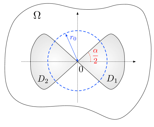
Figure 1: Setting of the bowtie-shaped domain presented in Section 2.3.

Remark 2.

We have assumed $D$ to be smooth except at the contact point $0$ between the wings $D_{1}$ and $D_{2}$. Our analysis remains valid if $D_{1}$ and $D_{2}$ have additionnal corners (for instance if they are shaped as triangles, as is often the case in actual physical devices). Indeed, as we show below, it is the contact point between the two wings that carries the worst singularity and determines the width of the essential spectrum of the Poincaré variational operator of $D$.

2.3.2 The Poincaré variational operator of a bowtie-shaped antenna

The bowtie-shaped domain $D$ of Section 2.3 fails to be Lipschitz regular, since it does not arise as the subgraph of a Lipschitz function in the vicinity of the point $0$. Rather than defining and studying an adapted Neumann-Poincaré operator (see [3] however for a related construction), we base our study of the well-posedness of (2.1) on the Poincaré variational operator, whose definition (2.5) naturally makes sense in the case of domains like $D$.

Since the set $D$ is not Lipschitz regular, some care is in order about the definition of the attached functional spaces. We denote by $H^{1}(D)$ is the set of functions on $D$ which are restrictions to $D$ of functions in $H^{1}({\mathbf{R}}^{2})$ and by $H^{1}_{0}(D)$ the closure of ${\mathcal{C}}^{\infty}_{c}(D)$ in $H^{1}_{0}(\Omega)$. Also, $\widetilde{H}^{1}(D)$ is the set of functions $u\in H^{1}(D)$ whose extension to $\Omega$ by $0$ is in $H^{1}_{0}(\Omega)$. Let us recall that, if ${\mathcal{O}}\Subset\Omega$ is a Lipschitz domain $\widetilde{H}^{1}({\mathcal{O}})=H^{1}_{0}({\mathcal{O}})$; see [28]. Unfortunately, the bowtie-shaped domain $D$ is not Lipschitz, but this property nevertheless holds, as we now prove:

Lemma 1.

Let $D$ be a bowtie as described in Section 2.3.1. Then $\widetilde{H}^{1}(D)=H^{1}_{0}(D)$.

Proof.

On the one hand, any smooth function in ${\mathcal{C}}^{\infty}_{c}(D)$ can be extended by $0$ to a function in $H^{1}_{0}(\Omega)$, so that by density, $H^{1}_{0}(D)\subset\widetilde{H}^{1}(D)$ (this inclusion actually holds true in the case of a general domain $D$).

On the other hand, to show the reverse inclusion, let $u\in\widetilde{H}^{1}(D)$; given the particular shape of $D$, one may write $u=u_{1}+u_{2}$, for some $u_{1},u_{2}\in H^{1}(D)$ with $\textrm{Supp}(u_{1})\subset D_{1}$ and $\textrm{Supp}(u_{2})\subset D_{2}$. Since $D_{1}$ is a Lipschitz domain, $u_{1}\in\widetilde{H}^{1}(D_{1})=H^{1}_{0}(D_{1})$ and $u_{1}$ arises as the limit in $H^{1}_{0}(\Omega)$ of a sequence of functions $u_{1,n}\in{\mathcal{C}}^{\infty}_{c}(D_{1})$; hence $u_{1}\in H^{1}_{0}(D)$. Similarly, $u_{2}\in H^{1}_{0}(D)$, so that $\widetilde{H}^{1}(D)\subset H^{1}_{0}(D)$. ∎

The main spectral properties of $T_{D}$ are described in the following proposition, which is an echo of Proposition 2 in the case of the bowtie-shaped domain $D$. The proof is essentially that of Proposition 3.2 in [13], except for a technical point that we make precise.

Proposition 3.

The operator $T_{D}$ is bounded, self-adjoint, with operator norm $||T_{D}||=1$. Moreover,

• Its spectrum $\sigma(T_{D})$ is contained in the interval $[0,1]$.

• The eigenspace associated to the eigenvalue $0$ is:

  $${\text{\rm Ker}}(T_{D}) = \{u\in H^{1}_{0}(\Omega),\>\exists c\in{\mathbf{R}},\>u=c\text{ in }D\}.$$

• The value $1$ belongs to $\sigma(T_{D})$ and the associated eigenspace is

  $${\text{\rm Ker}}({\text{\rm Id}}-T_{D}) = \{u\in H^{1}_{0}(\Omega),u=0\;\textrm{ in }\Omega\setminus\overline{D}\};$$

  therefore, in light of Lemma 1, ${\text{\rm Ker}}({\text{\rm Id}}-T_{D})$ is naturally identified with $H^{1}_{0}(D)$.

• The space $H^{1}_{0}(\Omega)$ decomposes as

  $$H^{1}_{0}(\Omega) = {\text{\rm Ker}}(T_{D})\oplus{\text{\rm Ker}}({\text{\rm Id}}-T_{D})\oplus{\mathcal{H}}_{D},$$

  where ${\mathcal{H}}_{D}$ is the closed subspace of $H^{1}_{0}(\Omega)$ defined by

  $${\mathcal{H}}_{D} = \left\{u\in H^{1}_{0}(\Omega),\>\Delta u=0\;\textrm{in}\;D\cup(\Omega\setminus\overline{D})\text{ and }{\displaystyle}\int_{\partial D_{1}\cup\partial D_{2}}{\displaystyle}\frac{\partial u^{+}}{\partial\nu}\,ds=0\right\}.$$ (2.11)

Proof.

(i): It is a straightforward consequence of the self-adjointness of $T_{D}$ and of the fact that $\lvert\lvert T_{D}\lvert\lvert=1$.

(ii): By definition, a function $u\in H^{1}_{0}(\Omega)$ belongs to ${\text{\rm Ker}}(T_{D})$ if and only if

$$\forall v\in H^{1}_{0}(\Omega),\>\>\int_{D}{\nabla u\cdot\nabla v\>dx}=0.$$

Let $u\in{\text{\rm Ker}}(T_{D})$; then $\int_{D}{\lvert\nabla u\lvert^{2}\>dx}=0$, so that $u$ is constant on $D_{1}$ and on $D_{2}$: there exist $c_{1}$, $c_{2}\in{\mathbf{R}}$ such that $u=c_{i}$ on $D_{i}$, $i=1,2$. Moreover, since $u\in H^{1}_{0}(\Omega)$, the trace $u\lvert_{\ell}$ of $u$ on the one-dimensional subset $\ell:=\left\{x=(x_{1},x_{2})\in\Omega,\>x_{2}=0\right\}$ belongs to $H^{\frac{1}{2}}(\ell)$. However, by the definition of $u$ and $D$, there exists $r_{0}>0$ such that:

$$u\lvert_{\ell}(x)=c_{1}\text{ if }x=(x_{1},0)\text{ with }-r_{0}<x_{1}<0\text{ and }u\lvert_{\ell}(x)=c_{2}\text{ if }x=(x_{1},0)\text{ with }0<x_{1}<r_{0}.$$

This implies that $c_{1}=c_{2}$. Conversely, if $u\in H^{1}_{0}(\Omega)$ satisfies $u=c$ on $D$ for some $c\in{\mathbf{R}}$, then $u\in{\text{\rm Ker}}(T_{D})$.

(iii): This follows from a similar argument.

(iv): A function $u\in H^{1}_{0}(\Omega)$ is orthogonal to ${\text{\rm Ker}}(T_{D})$ if and only if

$$\forall v\in{\text{\rm Ker}}(T_{D}),\>\>\int_{\Omega}{\nabla u\cdot\nabla v\>dx}=0.$$ (2.12)

Using first test functions $v\in{\mathcal{C}}^{\infty}_{c}(\Omega\setminus\overline{D})$, we obtain that $\Delta u=0$ in $\Omega\setminus\overline{D}$. Now using arbitrary functions $v\in H^{1}_{0}(\Omega)$ take a constant value inside $D$, and integrating by parts yields the subsequent condition:

$$\int_{\partial D_{1}\cup\partial D_{2}}{\frac{\partial u^{+}}{\partial n}\>ds}=0.$$ (2.13)

Eventually, one proves in a similar way that $u\in H^{1}_{0}(\Omega)$ is orthogonal to ${\text{\rm Ker}}({\text{\rm Id}}-T_{D})$ if and only if $\Delta u=0\text{ in }D$. ∎

Remark 3.

• Rigorously speaking, the definition of the normal derivative $\frac{\partial u^{+}}{\partial\nu}$ as an element in $H^{-1/2}(\partial D)$ in (2.11) is not so straightforward in the present context, since $D$ fails to be Lipschitz. It is possible to define this notion nevertheless, but we shall not require this in the present article; for our purpose, we may understand (2.13) in the sense that (2.12) holds for any function $v\in H^{1}_{0}(\Omega)$ such that $v\equiv 1$ on $D$.

• Interestingly, from the vantage of the eigenspaces of $T_{D}$, $D$ behaves as if it were a connected domain (compare Proposition 3 with its the counterpart Proposition 2 in the Lipschitz case). This peculiarity highlights one specificity of bowtie-shaped domains.

3 Corner singularity functions for a bowtie

In this section we characterize the local behavior of solutions to the equation

$$\textrm{div}(a\nabla u)=0,\text{ where }a(x)\text{ is given by (\ref{def_a}),}$$ (3.1)

in the vicinity of the contact point $x=0$ of the two wings of the bowtie $D$.

When $k$ takes a positive real value, this question pertains to the theory of elliptic corner singularity, to which a great deal of literature is devoted, see e.g. [35, 28, 22, 23, 36]. In a nutshell, for a two-phase transmission problem of the form (3.1) featuring a piecewise smooth inclusion with corners, $u$ is expected to decompose as the sum of a regular and of a singular part $u=u_{\text{\rm reg}}+u_{\text{\rm sing}}$, where $u_{\text{\rm reg}}$ has at least $H^{2}$ regularity, whereas $u_{\text{\rm sing}}$ is $H^{1}$ but not $H^{2}$ regular. Moreover, in the neighborhood of a corner, the latter function takes the following form in polar coordinates:

$$u_{\text{\rm sing}}(r,\theta) = Cr^{\eta}{\varphi}(\theta).$$

In this expression, $C$ is a multiplicative constant, $\eta\in(0,1]$ and ${\varphi}$ is a piecewise smooth function; both $\eta$ and ${\varphi}$ depend on the geometry of the wedge and of the contrast in conductivities.

In the present section, we investigate the local behavior of the non trivial solutions to (3.1) in the case of a bowtie-shaped domain $D$, when $k$ takes negative values. More precisely, let the conductivity $a$ be defined by:

$$a(\theta) := \left\{\begin{array}[]{ll}k&\textrm{if}\;|\theta|<\frac{{\alpha}}{2}\;\textrm{or}\;|\pi-\theta|<\frac{{\alpha}}{2}\\ 1&\textrm{otherwise}.\end{array}\right.$$

We search for a solution to (3.1) in the whole space ${\mathbf{R}}^{2}$. More specifically, we are interested in finding some solutions to (3.1) in the sense of distributions which do not belong to the energy space $H^{1}_{\text{\rm loc}}({\mathbf{R}}^{2})$. These solutions will be the key ingredient in the construction of generalized eigenfunctions of $T_{D}$ carried out in Section 4. Considering the symmetry of the geometric configuration with respect to the horizontal axis, it is enough to search for solutions $u$ to one of the following two problems set on the upper half-space $\Pi^{+}:=\left\{x=(x_{1},x_{2})\in{\mathbf{R}}^{2},\>\>x_{2}>0\right\}$:

$$\left\{\begin{array}[]{ccll}\textrm{div}(a\nabla u)&=&0&\textrm{in}\;\Pi^{+}\\ u(x)&=&0&\text{on }\partial\Pi^{+},\end{array}\right.$$ (3.5)

$$\left\{\begin{array}[]{ccll}\textrm{div}(a\nabla u)&=&0&\textrm{in}\;\Pi^{+}\\ \frac{\partial u}{\partial n}(x)&=&0&\text{on }\partial\Pi^{+}.\end{array}\right.$$ (3.8)

Indeed, assume that $u_{D}$ is a solution to (3.5) in the sense of distributions, and define

$$u(x_{1},x_{2})=\left\{\begin{array}[]{cl}u_{D}(x_{1},x_{2})&\text{if }x_{2}\geq 0,\\ -u_{D}(x_{1},-x_{2})&\text{if }x_{2}<0,\end{array}\>\>\text{a.e. }x=(x_{1},x_{2})\in{\mathbf{R}}^{2}.\right.$$

Then it is easily seen that $u$ is a solution to (3.1) in the sense of distributions. Likewise, if $u_{N}$ is a solution to (3.8), then

$$u(x_{1},x_{2}):=\left\{\begin{array}[]{cl}u_{N}(x_{1},x_{2})&\text{if }x_{2}\geq 0,\\ u_{N}(x_{1},-x_{2})&\text{if }x_{2}<0.\end{array}\right.$$

solves (3.1).

Let us first search for a solution to (3.5) under the form $u(r,\theta)=r^{i\xi}{\varphi}(\theta)$ for some $\xi>0$ and some function $\varphi(\theta)$ which is $2\pi$-periodic. Simple calculations show that (3.5) implies:

$$(a(\theta){\varphi}^{\prime}(\theta))^{\prime}-\xi^{2}a(\theta){\varphi}(\theta)\;=\;0$$

and so ${\varphi}$ has the form:

$${\varphi}(\theta) = \left\{\begin{array}[]{ll}a_{1}\cosh(\xi\theta)+b_{1}\sinh(\xi\theta)&\quad 0<\theta<\frac{{\alpha}}{2},\\ a_{2}\cosh(\xi\theta)+b_{2}\sinh(\xi\theta)&\quad\frac{{\alpha}}{2}<\theta<\pi-\frac{{\alpha}}{2},\\ a_{3}\cosh(\xi\theta)+b_{3}\sinh(\xi\theta)&\quad\pi-\frac{{\alpha}}{2}<\theta<\pi,\end{array}\right.$$

for some constants $a_{j}$, $b_{j}$, $j=1,2,3$ to be determined. Now expressing the transmission and boundary conditions in (3.5) yields a homogeneous linear system for the coefficients $a_{j},$ $b_{j}$. Existence of a non-trivial solution to (3.5) requires that the determinant of this system should vanish. A straightforward calculation shows that the latter determinant is the following polynomial of order $2$ in $k$:

$$d_{D}(k)=\cosh^{2}(\xi{\alpha}/2)\sinh[\xi(\pi-{\alpha})]k^{2}+\cosh^{2}[\xi(\pi-{\alpha})]\sinh(\xi{\alpha})k+\sinh^{2}(\xi{\alpha}/2)\sinh[\xi(\pi-{\alpha})],$$ (3.10)

in which $\xi$ acts as a parameter. The roots of $d_{D}(k)$ are:

$$k_{D,+}(\xi)={\displaystyle}\frac{-\left(\cosh[\xi(\pi-{\alpha})]-1\right)\sinh(\xi{\alpha})}{2\cosh^{2}(\xi{\alpha}/2)\sinh[\xi(\pi-{\alpha})]}\text{ and }k_{D,-}(\xi)={\displaystyle}\frac{-\left(\cosh[\xi(\pi-{\alpha})]+1\right)\sinh(\xi{\alpha})}{2\cosh^{2}(\xi{\alpha}/2)\sinh[\xi(\pi-{\alpha})]}.$$ (3.11)

Likewise, there exists a solution to (3.8) of the form $u=r^{i\xi}\varphi(\theta)$ provided the following determinant vanishes:

$$d_{N}(k)=\sinh^{2}(\xi{\alpha}/2)\sinh[\xi(\pi-{\alpha})]k^{2}+\cosh^{2}[\xi(\pi-{\alpha})]\sinh(\xi{\alpha})k+\cosh^{2}(\xi{\alpha}/2)\sinh[\xi(\pi-{\alpha})].$$ (3.12)

Its roots are:

$$k_{N,+}(\xi)={\displaystyle}\frac{-\left(\cosh[\xi(\pi-{\alpha})]-1\right)\sinh(\xi{\alpha})}{2\sinh^{2}(\xi{\alpha}/2)\sinh[\xi(\pi-{\alpha})]}\text{ and }k_{N,-}(\xi)={\displaystyle}\frac{-\left(\cosh[\xi(\pi-{\alpha})]+1\right)\sinh(\xi{\alpha})}{2\sinh^{2}(\xi{\alpha}/2)\sinh[\xi(\pi-{\alpha})]}.$$

It is easy to check that $k_{D,+}$ is a smooth function on ${\mathbf{R}}_{+}$, that $\lim_{\xi\to 0^{+}}k_{D,+}(\xi)=0$, while $\lim_{\xi\to+\infty}k_{D,+}(\xi)=-1$. In addition, we may rewrite:

$$k_{D,+}(\xi) = \left(-{\displaystyle}\frac{\cosh[\xi(\pi-{\alpha})]-1}{\sinh[\xi(\pi-a)]}\right)\tanh(\xi{\alpha}/2),$$

and check that as functions of $\xi>0$, the first term in the above right-hand side is negative and decreasing, while the second is positive and increasing. We conclude that $k_{D,+}(\xi)$ is a decreasing function that maps $(0,\infty)$ into $(0,-1)$.

On the other hand, $k_{N,-}$ is a smooth function on ${\mathbf{R}}_{+}$, $\lim_{\xi\to 0^{+}}k_{N,-}(\xi)=-\infty$, $\lim_{\xi\to+\infty}k_{N,-}(\xi)=-1$, and it holds:

$$k_{N,-}(\xi) = \left(-{\displaystyle}\frac{\cosh[\xi(\pi-{\alpha})]+1}{\sinh[\xi(\pi-a)]}\right)\tanh^{-1}(\xi{\alpha}/2),$$

As functions of $\xi>0$, the first term in the above right-hand side is negative and increasing, while the second is positive and decreasing. It follows that $k_{N,-}$ is a strictly increasing function of $\xi$ that maps $(0,\infty)$ into $(-\infty,-1)$.

Thus, for any $-1<k<0$ (resp. $-\infty<k<-1$) there exists a unique $\xi$ such that $k=k_{D,+}(\xi)$ (resp. $k=k_{N,-}(\xi))$. We also note that $k_{D,\pm}$ and $k_{N,\pm}$ are even functions of $\xi\in{\mathbf{R}}$, so that if $u=r^{i\xi}{\varphi}(\theta)$ is a singular solution, so is $r^{-i\xi}{\varphi}(\theta)$.

We summarize our findings in a technical lemma:

Lemma 2.

For any $k<0$, $k\neq-1$, there exists $\xi>0$ and a $2\pi$-periodic function $\varphi\in H^{1}_{\#}(0,2\pi)$ such that the function $u$ defined by

$$u(x_{1},x_{2})={\text{\rm Re}}(r^{i\xi}\varphi(\theta))\in L^{\infty}(\Omega)$$ (3.13)

is a solution of (3.1) in the sense of distributions. In addition, the function $\varphi$ in (3.13) solves

$$(a(\theta){\varphi}^{\prime}(\theta))^{\prime}-\xi^{2}a(\theta){\varphi}(\theta)=0.$$

Remark 4.

• One can check that $k_{N,-}(\xi)<k_{N,+}(\xi)<-1<k_{D,-}(\xi)<k_{D,+}(\xi)<0$ for all $\xi>0$.

• In the case where $k>0$, the same procedure yields solutions of (3.1) of the form $u(r,\theta)=r^{\xi}{\varphi}(\theta)$ for some $0<\xi<1$ and $\varphi\in H^{1}_{\#}(0,2\pi)$; such functions are in $H^{1}_{\text{\rm loc}}({\mathbf{R}}^{2})\setminus H^{2}_{\text{\rm loc}}({\mathbf{R}}^{2})$.

4 Characterization of the spectrum of $T_{D}$

In this section, we now proceed to the identification of the spectrum of $T_{D}$.

Theorem 1.

The operator $T_{D}$ has only essential spectrum and

$$\sigma(T_{D}) = [0,1].$$

Proof.

Using Proposition 3 and the fact that $\sigma_{\text{\rm ess}}(T_{D})$ is closed, it is enough to show that any number $\beta\in(0,1)$, $\beta\neq\frac{1}{2}$ lies in the essential spectrum of $T_{D}$. The proof relies on the same ingredients as that of Theorem 2 in [18] and we reproduce it for the sake of completeness.

Step 1: Using the singular solutions $u$ to the transmission problem (3.1) (see Lemma 2) calculated in the previous section, we aim at constructing a singular Weyl sequence for the operator $T_{D}$ and the value $\beta$, namely, a sequence of functions $u_{\varepsilon}\in H^{1}_{0}(\Omega)$ satisfying the following properties (see Section A):

$$\left\{\begin{array}[]{ccll}||u_{\varepsilon}||_{H^{1}_{0}(\Omega)}&=&1,\\ (\beta{\text{\rm Id}}-T_{D})u_{\varepsilon}&\to&0&\textrm{strongly in}\;H^{1}_{0}(\Omega),\\ u_{\varepsilon}&\to&0&\textrm{weakly in}\;H^{1}_{0}(\Omega).\end{array}\right.$$ (4.1)

To this end, let $\rho<\frac{r_{0}}{2}$; we introduce two smooth cut-off functions $\chi_{1},\chi_{2}:{\mathbf{R}}^{+}\rightarrow[0,1]$ such that for some constant $C>0$, the following relations hold:

$$\begin{array}[]{lll}\chi_{1}(s)=0\text{ for }|s|\leq 1,&\chi_{1}(s)=1\text{ for }|s|\geq 2,&|\chi_{1}^{\prime}(s)|\leq C\text{ for }s\geq 0,\\ \chi_{2}(s)=1\text{ for }|s|\leq\rho,&\chi_{2}(s)=0\text{ for }|s|\geq 2\rho,&|\chi_{2}^{\prime}(s)|\leq C\text{ for }s\geq 0.\end{array}$$ (4.2)

For ${\varepsilon}>0$ small enough, we set $\chi_{1}^{\varepsilon}(r)=\chi_{1}(\frac{r}{{\varepsilon}})$, and define

$$u_{\varepsilon}(x) = s_{\varepsilon}\chi^{\varepsilon}_{1}(r)\chi_{2}(r)u(x),\quad x\in\Omega,$$ (4.3)

where the normalization constant $s_{\varepsilon}$ is chosen so that $\lvert\lvert u_{\varepsilon}\lvert\lvert_{H^{1}_{0}(\Omega)}=1$.

Step 2: We estimate the constant $s_{\varepsilon}$. To this end, we decompose

$$\int_{\Omega}{\lvert\nabla u_{\varepsilon}\lvert^{2}\>dx}=s_{\varepsilon}^{2}(J_{1,\varepsilon}+m_{\varepsilon}+J_{2}),$$ (4.4)

where

$$J_{1,{\varepsilon}}=\int_{B_{2{\varepsilon}}\setminus\overline{B_{\varepsilon}}}{\lvert\nabla u_{\varepsilon}\lvert^{2}\>dx}=\int_{B_{2{\varepsilon}}\setminus\overline{B_{\varepsilon}}}{\lvert u\nabla\chi_{1}^{\varepsilon}+\chi_{1}^{\varepsilon}\nabla u\lvert^{2}\>dx},$$

$$m_{\varepsilon}=\int_{B_{\rho}\setminus\overline{B_{2{\varepsilon}}}}{\lvert\nabla u_{\varepsilon}\lvert^{2}\>dx}=\int_{B_{\rho}\setminus\overline{B_{2{\varepsilon}}}}{\lvert\nabla u\lvert^{2}\>dx},$$

and

$$J_{2}=\int_{B_{2\rho}\setminus\overline{B_{\rho}}}{\lvert\nabla u_{\varepsilon}\lvert^{2}\>dx}=\int_{B_{2\rho}\setminus\overline{B_{\rho}}}{\lvert\chi_{2}\nabla u+u\nabla\chi_{2}\lvert^{2}\>dx}.$$

Let us first estimate $J_{1,{\varepsilon}}$, using the explicit form (3.13) for $u$ and a change in polar coordinates:

$$\begin{array}[]{>{\displaystyle}cc>{\displaystyle}l}J_{1,{\varepsilon}}&=&\int_{{\varepsilon}}^{2{\varepsilon}}{\int_{0}^{2\pi}{\left(\left\lvert\frac{1}{\varepsilon}\frac{r^{i\xi}+r^{-i\xi}}{2}\varphi(\theta)\chi_{1}^{\prime}(\frac{r}{{\varepsilon}})+i\xi\frac{r^{i\xi}-r^{-i\xi}}{2r}\varphi(\theta)\chi_{1}(\frac{r}{{\varepsilon}})\right\lvert^{2}+\left\lvert\frac{r^{i\xi}+r^{-i\xi}}{2r}\varphi^{\prime}(\theta)\chi_{1}(\frac{r}{{\varepsilon}})\right\lvert^{2}\right)rdr}\>d\theta}\\ \hfil&\leq&\frac{C}{\varepsilon^{2}}\int_{{\varepsilon}}^{2{\varepsilon}}{\int_{0}^{2\pi}{r\>dr}\>d\theta}+C\int_{{\varepsilon}}^{2{\varepsilon}}{\int_{0}^{2\pi}{\frac{1}{r}\>dr}\>d\theta},\\ \hfil&\leq&C.\end{array}$$

In the above equation, and throughout the proof, $C$ is a generic constant independent of $\varepsilon$, which may change from one line to the next.

The integral $J_{2}$ does not depend on ${\varepsilon}$, and since $u$ is smooth on $B_{2\rho}\setminus\overline{B_{\rho}}$, it is bounded by some constant $C>0$.

Finally, since $u$ does not belong to $H^{1}_{0}(\Omega)$ (recall from (3.13) that its gradient blows up like $r^{-1}$ as $r\to 0$), it follows that

$$m_{\varepsilon}\xrightarrow{{\varepsilon}\to 0}\infty.$$ (4.5)

Let us note for further reference that the behavior of $m_{\varepsilon}$ as ${\varepsilon}\to 0$ may be estimated more precisely:

$$\begin{array}[]{>{\displaystyle}cc>{\displaystyle}l}m_{\varepsilon}&=&\int_{2{\varepsilon}}^{\rho}{\int_{0}^{2\pi}{\left(\xi^{2}\left\lvert\frac{r^{i\xi}-r^{-i\xi}}{2r}\varphi(\theta)\right\lvert^{2}+\frac{1}{r^{2}}\left\lvert\frac{r^{i\xi}+r^{-i\xi}}{2}\varphi^{\prime}(\theta)\right\lvert^{2}\right)}rdrd\theta},\\ \hfil&\leq&C\int_{2{\varepsilon}}^{\rho}{\int_{0}^{2\pi}{\frac{1}{r}}drd\theta},\end{array}$$

and so there exists a constant $C>0$ such that

$$m_{\varepsilon}\leq C\lvert\log{\varepsilon}\lvert.$$ (4.6)

Recalling (4.4), we obtain

$$1=s_{\varepsilon}^{2}m_{\varepsilon}(1+\frac{J_{1,{\varepsilon}}+J_{2}}{m_{\varepsilon}}),$$

so that there exists a constant $C>0$ such that

$$\frac{1}{C}m_{\varepsilon}^{-\frac{1}{2}}\leq s_{\varepsilon}\leq Cm_{\varepsilon}^{-\frac{1}{2}}.$$ (4.7)

Step 3: We show that $u_{\varepsilon}$ is a Weyl sequence for the operator $T_{D}$ and the value $\beta$. To this end, we estimate

$$\lvert\lvert\beta u_{\varepsilon}-T_{D}u_{\varepsilon}\lvert\lvert_{H^{1}_{0}(\Omega)}=\sup\limits_{v\in H^{1}_{0}(\Omega),\atop\lvert\lvert v\lvert\lvert_{H^{1}_{0}(\Omega)}=1}{J(v)},\text{ where }J(v):=\int_{\Omega}{\nabla(\beta u_{\varepsilon}-T_{D}u_{\varepsilon})\cdot\nabla v\>dx}.$$

Recall from (2.6) the alternative expression for $J(v)$

$$\begin{array}[]{>{\displaystyle}cc>{\displaystyle}l}J(v)&=&\beta\int_{\Omega\setminus\overline{D}}{\nabla u_{\varepsilon}\cdot\nabla v\>dx}+(\beta-1)\int_{D}{\nabla u_{\varepsilon}\cdot\nabla v\>dx}\\ \hfil&=&\beta\int_{\Omega}{a(x)\nabla u_{\varepsilon}\cdot\nabla v\>dx},\end{array}$$

with

$$a(x)=\left\{\begin{array}[]{cl}1&\text{if }x\in\Omega\setminus\overline{D},\\ 1-\frac{1}{\beta}&\text{if }x\in D.\end{array}\right.$$

Inserting the expression (4.3) of $u_{\varepsilon}$ in the definition of $J(v)$ yields after elementary calculations:

$$J(v) = s_{\varepsilon}\beta{\displaystyle}\int_{\Omega\setminus\overline{D}}{\nabla u\cdot\nabla(\chi_{1}^{\varepsilon}\chi_{2}v)\>dx}\;+\;s_{\varepsilon}(\beta-1){\displaystyle}\int_{D}{\nabla u\cdot\nabla(\chi_{1}^{\varepsilon}\chi_{2}v)\>dx}$$

$$\;+\;s_{\varepsilon}\beta{\displaystyle}\int_{\Omega\setminus\overline{D}}{u\nabla(\chi_{1}^{\varepsilon}\chi_{2})\cdot\nabla v\>dx}\;+\;s_{\varepsilon}(\beta-1){\displaystyle}\int_{D}{u\nabla(\chi_{1}^{\varepsilon}\chi_{2})\cdot\nabla v\>dx}$$

$$\;-\;s_{\varepsilon}\beta{\displaystyle}\int_{\Omega\setminus\overline{D}}{v\nabla u\cdot\nabla(\chi_{1}^{\varepsilon}\chi_{2})\>dx}\;-\;s_{\varepsilon}(\beta-1){\displaystyle}\int_{D}{v\nabla u\cdot\nabla(\chi_{1}^{\varepsilon}\chi_{2})\>dx}.$$

Since $u$ satisfies (3.1) and since the test function $\chi_{1}^{\varepsilon}\chi_{2}v$ has compact support in $B_{\rho}\setminus B_{\varepsilon}$, the sum of the first two integrals in the right-hand side of the above identity vanishes, so that

$$J(v)=\beta s_{\varepsilon}(J_{3,\varepsilon}(v)+J_{4,\varepsilon}(v)),$$ (4.8)

where we have defined:

$$J_{3,{\varepsilon}}(v)=\int_{\Omega}{au\nabla(\chi_{1}^{\varepsilon}\chi_{2})\cdot\nabla v\>dx}-\int_{B_{2\rho}\setminus\overline{B_{\rho}}}{av\nabla u\cdot\nabla\chi_{2}\>dx},\text{~{} and }J_{4,{\varepsilon}}(v)=-\int_{B_{2{\varepsilon}}\setminus\overline{B_{\varepsilon}}}{av\nabla u\cdot\nabla\chi_{1}^{\varepsilon}\>dx}.$$ (4.9)

Similar calculations to those involved in the estimate (4.7) show that

$$|J_{3,{\varepsilon}}(v)|\leq C\,||v||_{H^{1}_{0}(\Omega)}\left(\frac{1}{\varepsilon^{2}}\int_{0}^{2{\varepsilon}}{\displaystyle}\int_{0}^{2\pi}{|u|^{2}|\chi_{1}^{\prime}|^{2}\,rdrd\theta}+\int_{\rho}^{2\rho}{\displaystyle}\int_{0}^{2\pi}\left(|u|^{2}|\chi_{2}^{\prime}|^{2}+|\nabla u|^{2}|\chi_{2}|^{2}\right)\,rdrd\theta\right),$$ (4.10)

and so

$$J_{3,{\varepsilon}}(v)\leq C\lvert\lvert v\lvert\lvert_{H^{1}_{0}(\Omega)},$$ (4.11)

To estimate the remaining term $J_{4,{\varepsilon}}(v)$, we further decompose

$$J_{4,{\varepsilon}}(v)=\int_{B_{2{\varepsilon}}\setminus\overline{B_{\varepsilon}}}{a\overline{v}\nabla u\cdot\nabla\chi_{1}^{\varepsilon}\>dx}+\int_{B_{2{\varepsilon}}\setminus\overline{B_{\varepsilon}}}{a(v-\overline{v})\nabla u\cdot\nabla\chi_{1}^{\varepsilon}\>dx},$$ (4.12)

where $\overline{v}:=\frac{1}{|B_{2{\varepsilon}}|}\int_{B_{2{\varepsilon}}}{v(x)\,dx}$. The first integral in the above right-hand side reduces to

$$\begin{array}[]{>{\displaystyle}cc>{\displaystyle}l}\int_{B_{2{\varepsilon}}\setminus\overline{B_{\varepsilon}}}{a\overline{v}\nabla u\cdot\nabla\chi_{1}^{\varepsilon}\>dx}&=&\frac{\overline{v}}{{\varepsilon}}\int_{{\varepsilon}}^{2{\varepsilon}}{\int_{0}^{2\pi}{a(\theta)\chi_{1}^{\prime}(\frac{r}{\varepsilon})\>i\xi\frac{r^{i\xi}-r^{-i\xi}}{2r}\varphi(\theta)}\>rdrd\theta},\\ \hfil&=&\frac{\overline{v}}{{\varepsilon}}\int_{0}^{2\pi}{a(\theta)\varphi(\theta)\>d\theta}\>\int_{\varepsilon}^{2{\varepsilon}}{i\xi\frac{r^{i\xi}-r^{-i\xi}}{2}\chi^{\prime}(\frac{r}{{\varepsilon}})\>dr},\\ \hfil&=&0,\end{array}$$

where we have used the fact that $\varphi\in H^{1}_{\#}(0,2\pi)$ is a solution to the equation:

$$(a(\theta){\varphi}^{\prime}(\theta))^{\prime}-\xi^{2}a(\theta){\varphi}(\theta)=0,$$

so that it satisfies $\int_{0}^{2\pi}a(\theta){\varphi}(\theta)\,d\theta=0$. Hence, returning to (4.12), it follows that

$$|J_{4,{\varepsilon}}(v)| \leq \left({\displaystyle}\int_{B_{2{\varepsilon}}\setminus\overline{B_{\varepsilon}}}a^{2}|\nabla u\cdot\nabla\chi_{\varepsilon}|^{2}\,dx\right)^{\frac{1}{2}}\left({\displaystyle}\int_{B_{2{\varepsilon}}}{|v-\overline{v}|^{2}dx}\right)^{\frac{1}{2}}.$$

The following Poincaré-Wirtinger inequality

$$\int_{B_{2{\varepsilon}}}{\lvert v-\overline{v}\lvert^{2}\>dx}\leq C\varepsilon^{2}\int_{B_{2{\varepsilon}}}{\lvert\nabla v\lvert^{2}\>dx},$$

where the constant $C$ is independent of ${\varepsilon}$, yields

$$\begin{array}[]{>{\displaystyle}cc>{\displaystyle}l}|J_{4,{\varepsilon}}(v)|&\leq&C{\varepsilon}||v||_{H^{1}_{0}(\Omega)}\left(\int_{0}^{2\pi}a(\theta)^{2}|{\varphi}(\theta)|^{2}\,d\theta\right)^{1/2}\quad\left(\int_{{\varepsilon}}^{2{\varepsilon}}{\left\lvert i\xi{\displaystyle}\frac{r^{i\xi}-r^{-i\xi}}{2r}\right\lvert^{2}\frac{1}{{\varepsilon}^{2}}\chi_{1}^{\prime}(\frac{r}{{\varepsilon}})^{2}\,rdr}\right)^{1/2}\\ \hfil&\leq&C||v||_{H^{1}_{0}(\Omega)}\left({\displaystyle}\int_{{\varepsilon}}^{2{\varepsilon}}{\frac{dr}{r}}\right)^{1/2}\\ \hfil&\leq&C||v||_{H^{1}_{0}(\Omega)}.\end{array}$$

We conclude from (4.8), (4.10) and the above estimate that

$$\lvert J(v)\lvert\leq Cs_{\varepsilon}\lvert\lvert v\lvert\lvert_{H^{1}_{0}(\Omega)}.$$

Since $s_{\varepsilon}\to 0$ (see (4.7) and (4.5)), this proves that

$$\lvert\lvert\beta u_{\varepsilon}-T_{D}u_{\varepsilon}\lvert\lvert_{H^{1}_{0}(\Omega)}\xrightarrow{{\varepsilon}\to 0}0,$$

and so $u_{\varepsilon}$ is a Weyl sequence for $T_{D}$ and the value $\beta$.

Step 4: Finally, we show that $u_{\varepsilon}$ is a singular Weyl sequence for $T_{D}$ and the value $\beta$, namely that $u_{\varepsilon}\to 0$ weakly in $H^{1}_{0}(\Omega)$. Since $u_{\varepsilon}$ has unit norm in $H^{1}_{0}(\Omega)$, it is enough to prove that $u_{\varepsilon}\to 0$ strongly in $L^{2}(\Omega)$, which follows easily from (4.3), from the boundedness of $\chi_{1}^{\varepsilon}$, $\chi_{2}$ and $u$ in $L^{\infty}(\Omega)$, and from the fact that $s_{\varepsilon}\to 0$ (viz. (4.7)).

∎

5 Comparison with the bowtie with close-to-touching wings

It is interesting to compare the spectral properties of the Poincaré variational operator of $D$ to that of a (Lipschitz) domain $D_{\delta}=D_{1,{\delta}}\cup D_{2,{\delta}}$ with only close-to-touching wings. Let us introduce

$$D_{1,{\delta}}\;=\;({\delta}/2,0)+D_{1}, D_{2,{\delta}}\;=\;(-{\delta}/2,0)+D_{2},$$

where the parameter ${\delta}>0$ is sufficiently small so that $D_{\delta}\Subset\Omega$; see Figure 2.

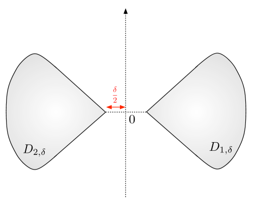
Figure 2: The bowtie with close-to-touching wings.

The corresponding Poincaré variational operator $T_{D_{\delta}}~{}:H^{1}_{0}(\Omega)\longrightarrow H^{1}_{0}(\Omega)$ is now defined by

$$\forall\;v\in H^{1}_{0}(\Omega),\quad{\displaystyle}\int_{\Omega}{\nabla(T_{D_{\delta}}u)\cdot\nabla v\>dx} = {\displaystyle}\int_{D_{\delta}}{\nabla u\cdot\nabla v\>dx}.$$

Since $D_{\delta}$ is Lipschitz regular, the study of the spectrum $\sigma(T_{D_{\delta}})$ falls into the framework of Sections 2.2.2 and 2.2.3, and Proposition 2 holds in this case.

More precisely, both domains $D_{1,\delta}$ and $D_{2,\delta}$ have a piecewise smooth boundary with a finite number of angles. Hence, the results of K.-M. Perfekt and M. Putinar [43] apply: the essential spectrum of the associated Poincaré variational operator $T_{D_{\delta}}$ (and that of the Neumann-Poincaré operator ${\mathcal{K}}_{D}^{*}$) is completely determined by the most acute angle $\alpha$ on the boundary of $D_{1,\delta}$ and $D_{2,\delta}$. In our context, this takes the form:

$$\sigma_{\text{\rm ess}}(T_{D_{\delta}})=\left[\frac{\alpha}{2\pi},1-\frac{\alpha}{2\pi}\right];\>\>\sigma_{\text{\rm ess}}({\mathcal{K}}^{*}_{D_{\delta}})=\left[-\frac{\pi-\alpha}{2\pi},\frac{\pi-\alpha}{2\pi}\right].$$

Hence, the close-to-touching corners of $D_{\delta}$ are qualitatively less singular than the bowtie feature of $D$, which is associated to an essential spectrum $\sigma(T_{D})=[0,1]$. A similar phenomenon was already noticed in the article [17], investigating the regularity of solutions to (2.1) in the case of the domains $D$ and $D_{\delta}$ for a value $k>0$ of the conductivity. In the close-to-touching case, the singular part of the solution $u_{\delta}$ to (2.1) behaves like $r^{\eta}$ at the vertices, with $\eta\geq 2/3$ independently of the value of $k$ and of the angle ${\alpha}$. For the touching case (i.e. in the case of $D$), $u$ behaves also like $r^{\eta}$ at the contact point, but $\eta$ can be made as close to $0$ as desired by choosing $k$ sufficiently close to $0$ or $+\infty$.

Our aim is now to shpw that, as ${\delta}\to 0$, the spectrum $\sigma(T_{D_{\delta}})$ converges to a limiting set which is exactly the spectrum $\sigma(T_{D})=[0,1]$ of the limiting physical situation. To this end, we study the limit spectrum

$$\lim\limits_{\delta\to 0}{\sigma(T_{D_{\delta}})}:=\left\{\beta\in\mathbb{R},\>\>\exists\delta_{n}\downarrow 0,\>\beta_{n}\in\sigma(T_{D_{\delta_{n}}}),\>\>\beta_{n}\to\beta\right\}$$ (5.1)

of the sequence of operators $T_{D_{\delta}}$.

Our analysis relies on the following abstract result for self-adjoint operators, which is part of the statement of Lemma (2.8) in [1].

Theorem 2.

Let $H$ be a Hilbert space and $S_{\delta}~{}:H\rightarrow H$ denote a sequence of self-adjoint operators, with spectrum $\sigma(S_{\delta})$. Assume that the operators $S_{\delta}$ converge pointwise to a limiting operator $S$, with spectrum $\sigma(S)$, in the sense that

$$\forall\;u\in H,\quad\lim_{\delta\to 0}||S_{\delta}u-Su|| \rightarrow 0.$$ (5.2)

Then,

$$\lim_{\delta\to 0}\sigma(S_{\delta}) \supset \sigma(S),$$ (5.3)

where the left-hand set denotes the limit spectrum of the sequence of operators $S_{\delta}$.

Remark 5.

The statement in [1] is more general; in this reference, the result is proved under the additional assumption that the operators $S_{\delta}$ and $S$ are compact, but this hypothesis is not necessary for the version presented in Theorem 2.

We now prove

Proposition 4.

The operators $T_{D_{\delta}}$ converge pointwise to $T_{D}$ as $\delta\to 0$, in the sense that

$$\forall\;u\in H^{1}_{0}(\Omega),\quad\lim_{\delta\to 0}||T_{D_{\delta}}u-T_{D}u||_{H^{1}_{0}(\Omega)}=0.$$

Proof: Fix $u\in H^{1}_{0}(\Omega)$ and consider

$$||T_{D_{\delta}}u-T_{D}u||_{H^{1}_{0}(\Omega)}^{2} = {\displaystyle}\int_{\Omega}|\nabla T_{D_{\delta}}{u-\nabla T_{D}u|^{2}\>dx}$$

$$= {\displaystyle}\int_{D_{\delta}}\nabla u\cdot\nabla\left(T_{D_{\delta}}u-T_{D}u\right)\>dx-{\displaystyle}\int_{D}\nabla u\cdot\nabla\left(T_{D_{\delta}}u-T_{D}u\right)\>dx$$

$$= {\displaystyle}\int_{\Omega}(\mathds{1}_{D_{\delta}}-\mathds{1}_{D})\nabla u\cdot\nabla\left(T_{D_{\delta}}u-T_{D}u\right)\>dx$$

$$\leq \left({\displaystyle}\int_{\Omega}(\mathds{1}_{D_{\delta}}-\mathds{1}_{D})|\nabla u|^{2}\>dx\right)^{1/2}||T_{D_{\delta}}u-T_{D}u||_{H^{1}_{0}(\Omega)}.$$

The Lebesgue Dominated Convergence Theorem shows that the first integral on the right-hand side tends to $0$ as ${\delta}\to 0$, which proves the Proposition.  

Combining Proposition 4, Theorem 2 and the fact that the spectrum of each $T_{D_{\delta}}$ is contained in $[0,1]$ (see Proposition 2), we obtain:

Corollary 1.

The limiting spectrum (5.1) of the operators $T_{D_{\delta}}$ is exactly that of the Poincaré variational operator of the bowtie antenna $D$:

$$\lim_{\delta\to 0}\sigma(T_{D_{\delta}})=\sigma(T_{D})=[0,1].$$

This result deserves a few additionnal comments. As we have mentionned, the essential spectrum of $T_{D_{\delta}}$ is exactly the interval $[{\displaystyle}\frac{{\alpha}}{2\pi},1-{\displaystyle}\frac{{\alpha}}{2\pi}]$ independently of $\delta$, whereas the above corollary shows that in the limit $\delta\to 0$, the spectrum $\sigma(T_{D_{\delta}})$ must densify so as to occupy the whole interval $[0,1]$. The only possible way for this to happen is that for ${\delta}$ sufficiently small $T_{D_{\delta}}$ must develop eigenvalues in the intervals $[0,{\displaystyle}\frac{\alpha}{2\pi})$ and $(1-{\displaystyle}\frac{{\alpha}}{2\pi},1]$, which become denser as $\delta\to 0$. Let us point out that such a densification phenomenon has been observed in different physical contexts; see  [31, 32] and [14].

6 Another approach to the limit spectrum of bowties with close-to-touching wings

The purpose of this section is to provide an alternative proof of the fact that $\sigma(T_{D_{\delta}})$ contains eigenvalues if the distance between the wings is sufficiently small. This fact is indeed contained in Corollary 1, but the forthcoming proof is more direct, and sheds light on the behavior of the eigenfunctions of $T_{D_{\delta}}$. The main result of this section is the following:

Theorem 3.

For ${\delta}>0$ small enough, the operator $T_{D_{\delta}}$ has eigenvalues in the range $\left(1-\frac{{\alpha}}{2\pi},1\right)$ and in the range $\left(0,\frac{{\alpha}}{2\pi}\right)$, i.e., outside the essential spectrum $\sigma_{\text{\rm ess}}(T_{D_{\delta}})$.

Proof.

Recalling the orthogonal decomposition (2.8), let us denote by $\beta_{{\delta}}^{-}$ and $\beta_{\delta}^{+}$ the lower and upper bounds of the spectrum of $T_{D_{\delta}}$ deprived of the trivial eigenvalues $0$ and $1$, i.e.

$$\beta_{\delta}^{-}=\inf_{\sigma(T_{D_{\delta}})\setminus\left\{0,1\right\}}\text{ and }\beta_{\delta}^{+}=\sup_{\sigma(T_{D_{\delta}})\setminus\left\{0,1\right\}}$$

Relying on a spectral representation for the operator $T_{D_{\delta}}:{\mathcal{H}}_{D_{\delta}}\to{\mathcal{H}}_{D_{\delta}}$ (see e.g. [44]), these bounds are given by the Rayleigh quotients:

$$\beta_{\delta}^{-}=\min\limits_{w\in H^{1}_{0}(\Omega)\atop w\perp{\text{\rm Ker}}(T_{D_{\delta}})}{\frac{\displaystyle{\int_{D_{\delta}}{\lvert\nabla w\lvert^{2}\>dx}}}{\displaystyle{\int_{\Omega}{\lvert\nabla w\lvert^{2}\>dx}}}}\;\text{ and }\;\beta_{\delta}^{+}=\max\limits_{w\in H^{1}_{0}(\Omega)\atop w\perp{\text{\rm Ker}}({\text{\rm Id}}-T_{D_{\delta}})}{\frac{\displaystyle{\int_{D_{\delta}}{\lvert\nabla w\lvert^{2}\>dx}}}{\displaystyle{\int_{\Omega}{\lvert\nabla w\lvert^{2}\>dx}}}}.$$ (6.1)

Let us now pick a value $\beta\notin[{\displaystyle}\frac{{\alpha}}{\pi},1-{\displaystyle}\frac{{\alpha}}{\pi}]$, so that $\beta$ lies outside the essential spectrum $\sigma_{\textrm{ess}}(T_{D_{\delta}})$ for any ${\delta}>0$. Our aim is to prove that there exists a sequence of functions $Z_{\delta}\in H^{1}_{0}(\Omega)$ which is orthogonal to ${\text{\rm Ker}}(T_{D_{\delta}})$ (resp. to ${\text{\rm Ker}}({\text{\rm Id}}-T_{D_{\delta}})$) such that:

$$\beta=\lim_{{\delta}\to 0}\frac{\displaystyle{\int_{D_{\delta}}{|\nabla Z_{\delta}|^{2}\>dx}}}{\displaystyle{\int_{\Omega}{|\nabla Z_{\delta}|^{2}\>dx}}}.$$

Let $k=1-{\displaystyle}\frac{1}{\beta}$ be the conductivity associated to $\beta$ (see Section 2.3.2). We take on the construction of $u_{\varepsilon}$ carried out in Section 4: let $u$ denote the function supplied by Lemma 2:

$$u(x) = {\text{\rm Re}}(r^{i\xi}){\varphi}(\theta),$$ (6.2)

where $\xi$ satisfies

$$d_{D}(\xi)=0 d_{N}(\xi)=0,$$ or

according to (3.10) and (3.12).

Let $0<\rho$ be sufficiently small, and let $\chi_{1}$, $\chi_{2}$ be the cut-off functions defined as in (4.2); for $0<{\varepsilon}<\rho$, we define:

$$u_{\varepsilon}(x) = s_{\varepsilon}\chi_{1}(\frac{r}{{\varepsilon}})\chi_{2}(r)u(x).$$

As in (4.3), the normalization constant $s_{\varepsilon}$ is chosen so that $||u_{\varepsilon}||_{H^{1}_{0}(\Omega)}=1$. Recall from (4.6) that there exists a constant $C>0$ such that:

$$s_{\varepsilon}\leq C{\displaystyle}\frac{1}{|\log({\varepsilon})|^{\frac{1}{2}}}.$$ (6.3)

The calculations performed in Section 4 have revealed that the sequence $u_{\varepsilon}$ satisfies

$$\lim_{{\varepsilon}\to 0}||(\beta I-T_{D})u_{\varepsilon}||_{H^{1}_{0}(\Omega)} = 0.$$ (6.4)

Recalling (2.5), this implies in particular that

$$\beta = \lim_{{\varepsilon}\to 0}\frac{\displaystyle{\int_{D}{|\nabla u_{\varepsilon}|^{2}\>dx}}}{\displaystyle{\int_{\Omega}{|\nabla u_{\varepsilon}|^{2}\>dx}}}\;=\;\lim_{{\varepsilon}\to 0}\int_{D}{|\nabla u_{\varepsilon}|^{2}\>dx}.$$ (6.5)

Let us next turn to the configuration $D_{\delta}$; for a small parameter $\varepsilon>0$ to be specified later, we define a function $v_{{\delta},{\varepsilon}}$ by:

$$v_{{\delta},{\varepsilon}}(x_{1},x_{2}) = \left\{\begin{array}[]{cl}u_{\varepsilon}(x_{1}+\frac{{\delta}}{2},x_{2})&\text{if }x_{1}<-\frac{{\delta}}{2},\\ u_{\varepsilon}(x_{1}-\frac{{\delta}}{2},x_{2})&\text{if }x_{1}>\frac{{\delta}}{2},\\ u_{\varepsilon}(0,x_{2})&\textrm{otherwise}.\end{array}\right.$$ (6.9)

Note that, by construction, $v_{{\delta},{\varepsilon}}\in H^{1}_{0}(\Omega)$ and:

$${\displaystyle}\int_{D_{\delta}}{|\nabla v_{{\delta},{\varepsilon}}|^{2}\>dx} = {\displaystyle}\int_{D}{|\nabla u_{\varepsilon}|^{2}\>dx}.$$ (6.10)

Additionnally, in view of (6.2), we have

$$\begin{array}[]{>{\displaystyle}cc>{\displaystyle}l}\int_{\Omega}{|\nabla v_{{\delta},{\varepsilon}}|^{2}\>dx}&=&\int_{x_{1}<-\frac{{\delta}}{2}}{|\nabla u_{\varepsilon}(x_{1}+\frac{{\delta}}{2},x_{2})|^{2}dx}+\int_{x_{1}>\frac{{\delta}}{2}}{|\nabla u_{\varepsilon}(x_{1}-\frac{{\delta}}{2},x_{2})|^{2}\>dx}+\int_{|x_{1}|<\frac{{\delta}}{2}}{|\partial_{x_{2}}u_{\varepsilon}(0,x_{2})|^{2}\>dx}\\ \hfil&=&\int_{\Omega}{|\nabla u_{\varepsilon}|^{2}\>dx}\;+\;s_{\varepsilon}^{2}\int_{|x_{1}|<\frac{{\delta}}{2}}{|\partial_{x_{2}}\left[\chi_{1}(\frac{x_{2}}{{\varepsilon}})\chi_{2}(x_{2})u(0,x_{2})\right]|^{2}\>dx}.\end{array}$$ (6.11)

We now estimate the last integral in the above expression; to this end,

$$\begin{array}[]{>{\displaystyle}cc>{\displaystyle}l}\int_{|x_{1}|<\frac{{\delta}}{2}}{\left\lvert\partial_{x_{2}}(\chi_{1}(\frac{x_{2}}{{\varepsilon}})\chi_{2}(x_{2})u(0,x_{2}))\right\lvert^{2}\>dx}&\leq&\frac{\delta}{{\varepsilon}^{2}}\int_{\varepsilon}^{2{\varepsilon}}{\left\lvert\chi_{1}^{\prime}(\frac{x_{2}}{{\varepsilon}})\chi_{2}(x_{2})\cos(\xi\log\lvert x_{2}\lvert)\right\lvert^{2}\>dx_{2}}\\ \hfil&&+\delta\int_{\rho}^{2\rho}{\left\lvert\chi_{1}(\frac{x_{2}}{{\varepsilon}})\chi_{2}^{\prime}(x_{2})\cos(\xi\log\lvert x_{2}\lvert)\right\lvert^{2}\>dx_{2}}\\ \hfil&&+{\delta}\int_{\varepsilon}^{2\rho}{\frac{\xi^{2}}{x_{2}^{2}}\left\lvert\chi_{1}(\frac{x_{2}}{{\varepsilon}})\chi_{2}(x_{2})\sin(\xi\log\lvert x_{2}\lvert)\right\lvert^{2}\>dx_{2}}.\\ \hfil&\leq&C\frac{{\delta}}{{\varepsilon}},\end{array}$$ (6.12)

where the constant $C>0$ is independent of ${\delta}$ and ${\varepsilon}$. Combining (6.10), (6.11) and (6.12), we find that

$$\frac{\displaystyle{\int_{D_{\delta}}|\nabla v_{{\delta},{\varepsilon}}|^{2}\>dx}}{\displaystyle{\int_{\Omega}{|\nabla v_{{\delta},{\varepsilon}}|^{2}\>dx}}} = {\displaystyle}\frac{\displaystyle{\int_{D}{|\nabla u_{\varepsilon}|^{2}\>dx}}}{\displaystyle{\int_{\Omega}{|\nabla u_{\varepsilon}|^{2}\>dx}}+\frac{s_{\varepsilon}^{2}{\delta}}{{\varepsilon}}B_{{\varepsilon},{\delta}}},$$

where $B_{{\varepsilon},{\delta}}$ is uniformly bounded with respect to ${\varepsilon}$ and ${\delta}$. Finally, choosing ${\varepsilon}={\delta}$ and using (6.5) and (6.3), it follows that the function $w_{\delta}:=v_{{\delta},{\delta}}$ satisfies

$$\left|\beta-{\displaystyle}\frac{\displaystyle{\int_{D_{\delta}}{|\nabla w_{\delta}|^{2}\>dx}}}{\displaystyle{\int_{\Omega}{|\nabla w_{\delta}|^{2}\>dx}}}\right| \leq {\displaystyle}\frac{C}{|\log{\delta}|}\to 0,\;\textrm{as}\;{\delta}\to 0.$$ (6.13)

On a different note, it will be useful for further purpose to notice that $w_{\delta}$ is somehow ‘close’ to $u_{\delta}$. More precisely, the following result will come in handy:

Lemma 3.

The following convergence holds:

$$\lvert\lvert u_{\delta}-w_{\delta}\lvert\lvert_{H^{1}_{0}(\Omega)}\to 0\text{ as }{\delta}\to 0.$$

The proof of Lemma 3 is technical and is postponed to the end of this section.

To summarize: we have constructed a series of ‘test’ functions $w_{\delta}\in H^{1}_{0}(\Omega)$ whose energy ratio converges to the desired value $\beta$ as ${\delta}\to 0$. To use these functions in the variational principles (6.1), we now construct from $w_{\delta}$ a new series of functions $Z_{\delta}\in H^{1}_{0}(\Omega)$ which satisfy the orthogonality conditions $Z_{\delta}\perp{\text{\rm Ker}}(T_{D_{\delta}})$ or $Z_{\delta}\perp{\text{\rm Ker}}({\text{\rm Id}}-T_{D_{\delta}})$. To achieve this, we separate both cases.

Case 1: $1-\frac{{\alpha}}{\pi}<\beta<1$.

Let $W_{\delta}$ denote the orthogonal projection of $w_{\delta}$ on ${\text{\rm Ker}}({\text{\rm Id}}-T_{D_{\delta}})=H^{1}_{0}(D_{\delta})$ and let $Z_{\delta}=w_{\delta}-W_{\delta}$. We also define the function:

$$U_{\delta}(x) = \mathds{1}_{\{x_{1}<0\}}(x)W_{\delta}(x_{1}-\frac{{\delta}}{2},x_{2})+\mathds{1}_{\{x_{1}>0\}}(x)W_{\delta}(x_{1}+\frac{{\delta}}{2},x_{2}).$$

Obviously, $\lvert\lvert U_{\delta}\lvert\lvert_{H^{1}_{0}(\Omega)}=\lvert\lvert W_{\delta}\lvert\lvert_{H^{1}_{0}(\Omega)}$. Also, since $W_{\delta}\in H^{1}_{0}(D_{\delta})$, there exists a sequence of smooth functions $(W_{n,{\delta}})_{n\geq 1}$ with compact support inside $D_{\delta}$ such that $W_{n,{\delta}}\to W_{\delta}$ strongly in $H^{1}_{0}(\Omega)$. It is then easy to check that the functions

$$U_{n,{\delta}}(x) := \mathds{1}_{\{x_{1}<0\}}(x)W_{n,{\delta}}(x_{1}-\frac{{\delta}}{2},x_{2})+\mathds{1}_{\{x_{1}>0\}}(x)W_{n,{\delta}}(x_{1}+\frac{{\delta}}{2},x_{2})$$

are smooth with compact support inside $D$ and that they satisfy $U_{n,{\delta}}\to U_{\delta}$ strongly in $H^{1}_{0}(\Omega)$. It follows that $U_{\delta}\in H^{1}_{0}(D)$.

Now, at first using (6.11), (6.12) and the orthogonality of $W_{\delta}$ and $Z_{\delta}$ yields:

$$\begin{array}[]{>{\displaystyle}cc>{\displaystyle}l}1+o(1)=\int_{\Omega}{\lvert\nabla w_{\delta}\lvert^{2}\>dx}&=&\int_{\Omega}{\lvert\nabla W_{\delta}\lvert^{2}\>dx}+\int_{\Omega}{\lvert\nabla Z_{\delta}\lvert^{2}\>dx}\\ \hfil&=&\int_{D_{\delta}}{\lvert\nabla W_{\delta}\lvert^{2}\>dx}+\int_{\Omega}{\lvert\nabla Z_{\delta}\lvert^{2}\>dx},\end{array}$$

where $o(1)\to 0$ as $\delta\to 0$. Also, from (6.13), using again (6.11) and (6.12), we infer:

$$\begin{array}[]{>{\displaystyle}cc>{\displaystyle}l}\beta+o(1)=\int_{D_{\delta}}{\lvert\nabla w_{\delta}\lvert^{2}\>dx}&=&\int_{D_{\delta}}{\lvert\nabla W_{\delta}\lvert^{2}\>dx}+\int_{D_{\delta}}{\lvert\nabla Z_{\delta}\lvert^{2}\>dx}+2\int_{D_{\delta}}{\nabla W_{\delta}\cdot\nabla Z_{\delta}\>dx}\\ \hfil&=&\int_{D_{\delta}}{\lvert\nabla W_{\delta}\lvert^{2}\>dx}+\int_{D_{\delta}}{\lvert\nabla Z_{\delta}\lvert^{2}\>dx},\\ \end{array}$$

since

$$\int_{D_{\delta}}{\nabla W_{\delta}\cdot\nabla Z_{\delta}\>dx}=\int_{\Omega}{\nabla(T_{D_{\delta}}W_{\delta})\cdot\nabla Z_{\delta}\>dx}=\int_{\Omega}{\nabla W_{\delta}\cdot\nabla Z_{\delta}\>dx}=0.$$

Hence, our purpose is now to prove that $\lvert\lvert W_{\delta}\lvert\lvert_{H^{1}_{0}(\Omega)}\to 0$ as ${\delta}\to 0$.

To this end, we first observe that, on the one hand, since $W_{\delta}\in{\text{\rm Ker}}({\text{\rm Id}}-T_{D_{\delta}})$,

$$\begin{array}[]{>{\displaystyle}cc>{\displaystyle}l}\int_{\Omega}{\nabla((T_{D_{\delta}}-\beta{\text{\rm Id}})w_{\delta})\cdot\nabla W_{\delta}\>dx}&=&\int_{\Omega}{\nabla w_{\delta}\cdot\nabla((T_{D_{\delta}}-\beta{\text{\rm Id}})W_{\delta})\>dx},\\ \hfil&=&(1-\beta)\int_{\Omega}{\nabla w_{\delta}\cdot\nabla W_{\delta}\>dx},\\ \hfil&=&(1-\beta)\lvert\lvert W_{\delta}\lvert\lvert^{2}_{H^{1}_{0}(\Omega)}.\end{array}$$ (6.14)

On the other hand, recalling (6.9) with ${\varepsilon}={\delta}$, a change of variables yields:

$$\begin{array}[]{>{\displaystyle}cc>{\displaystyle}l}\int_{\Omega}{\nabla(T_{D_{\delta}}w_{\delta})\cdot\nabla W_{\delta}\>dx}&=&{\displaystyle}\int_{D_{\delta}}{\nabla w_{\delta}\cdot\nabla W_{\delta}\>dx}\\ \hfil&=&{\displaystyle}\int_{D}{\nabla u_{\delta}\cdot\nabla U_{\delta}\>dx}\;=\;\int_{\Omega}{\nabla(T_{D}u_{\delta})\cdot\nabla U_{\delta}\>dx},\end{array}$$ (6.15)

and also, since $W_{\delta}$ and $U_{\delta}$ are supported in $D_{\delta}$ and in $D$ respectively,

$$\int_{\Omega}{\nabla w_{\delta}\cdot\nabla W_{\delta}\>dx} = {\displaystyle}\int_{D_{\delta}}{\nabla w_{\delta}\cdot\nabla W_{\delta}\>dx}\;=\;\int_{\Omega}{\nabla u_{\delta}\cdot\nabla U_{\delta}\>dx}.$$ (6.16)

Combining (6.15) and (6.16) thus implies:

$$\int_{\Omega}{\nabla((T_{D_{\delta}}-\beta{\text{\rm Id}})w_{\delta})\cdot\nabla W_{\delta}\>dx} = \int_{\Omega}{\nabla((T_{D}-\beta{\text{\rm Id}})u_{\delta})\cdot\nabla U_{\delta}\>dx}$$

$$\leq ||(T_{D}-\beta{\text{\rm Id}})u_{\delta}||_{H^{1}_{0}(\Omega)}||U_{\delta}||_{H^{1}_{0}(\Omega)}$$

$$= ||(T_{D}-\beta{\text{\rm Id}})u_{\delta}||_{H^{1}_{0}(\Omega)}||W_{\delta}||_{H^{1}_{0}(\Omega)}.$$

Combining this estimate with (6.14), and in view of (6.4), we obtain

$$(1-\beta)||W_{\delta}||_{H^{1}_{0}(\Omega)} \leq ||(T_{D}-\beta{\text{\rm Id}})u_{\delta}||_{H^{1}_{0}(\Omega)}\;=\;o(1)\quad\textrm{as}\;{\delta}\to 0.$$

Since $\beta\neq 1$, we conclude that $||W_{\delta}||_{H^{1}_{0}(\Omega)}\to 0$, as expected.

This together with (6.13) finally implies:

$$\beta=\lim_{{\delta}\to 0}\frac{\displaystyle{\int_{D_{\delta}}{|\nabla w_{\delta}|^{2}\>dx}}}{\displaystyle{\int_{\Omega}{|\nabla w_{\delta}|^{2}\>dx}}} = \lim_{{\delta}\to 0}\frac{\displaystyle{\int_{D_{\delta}}{|\nabla Z_{\delta}|^{2}\>dx}}}{\displaystyle{\int_{\Omega}{|\nabla Z_{\delta}|^{2}\>dx}}},$$

and so, since $Z_{\delta}\perp{\text{\rm Ker}}({\text{\rm Id}}-T_{D_{\delta}})$:

$$\beta_{\delta}^{+}=\max\limits_{w\in H^{1}_{0}(\Omega)\atop w\perp{\text{\rm Ker}}({\text{\rm Id}}-T_{D_{\delta}})}\frac{\displaystyle{\int_{D_{\delta}}{|\nabla w|^{2}\>dx}}}{\displaystyle{\int_{\Omega}{|\nabla w|^{2}\>dx}}} \geq \beta+o(1),$$ (6.17)

which is the desired result.

Case 2: $0<\beta<\frac{{\alpha}}{\pi}$.

Recalling (6.13), we again decompose $w_{\delta}=W_{\delta}+Z_{\delta}$, where $W_{\delta}$ now denotes the orthogonal projection of $w_{\delta}$ on ${\text{\rm Ker}}(T_{D_{\delta}})$, so that in particular $\nabla W_{\delta}=0$ inside $D_{\delta}$. Again, our aim is to prove that $W_{\delta}\to 0$ strongly in $H^{1}_{0}(\Omega)$ as ${\delta}\to 0$.

This follows from the chain of inequalities:

$$\begin{array}[]{>{\displaystyle}cc>{\displaystyle}l}||W_{\delta}||^{2}_{H^{1}_{0}(\Omega)}&=&{\displaystyle}\int_{\Omega}{\nabla W_{\delta}\cdot\nabla(w_{\delta}-Z_{\delta})\>dx}\\ \hfil&=&{\displaystyle}\int_{\Omega}{\nabla W_{\delta}\cdot\nabla w_{\delta}\>dx}\\ \hfil&=&{\displaystyle}\frac{1}{\beta}\,\int_{\Omega}{\nabla((\beta I-T_{D_{\delta}})u_{\delta})\cdot\nabla W_{\delta}\>dx}+\int_{\Omega}{\nabla(w_{\delta}-u_{\delta})\cdot\nabla W_{\delta}\>dx}+{\displaystyle}\frac{1}{\beta}\,\int_{\Omega}{\nabla T_{D_{\delta}}u_{\delta}\cdot\nabla W_{\delta}\>dx}\\ \hfil&\leq&{\displaystyle}\frac{1}{\beta}\,||(\beta I-T_{D_{\delta}})u_{\delta}||_{H^{1}_{0}(\Omega)}||W_{\delta}||_{H^{1}_{0}(\Omega)}+\lvert\lvert u_{\delta}-w_{\delta}\lvert\lvert_{H^{1}_{0}(\Omega)}\lvert\lvert W_{\delta}\lvert\lvert_{H^{1}_{0}(\Omega)}+{\displaystyle}\frac{1}{\beta}\left|{\displaystyle}\int_{D_{\delta}}{\nabla w_{\delta}\cdot\nabla W_{\delta}\>dx}\right|,\end{array}$$

and so:

$$\lvert\lvert W_{\delta}\lvert\lvert_{H^{1}_{0}(\Omega)}\leq{\displaystyle}\frac{1}{\beta}\,||(\beta I-T_{D_{\delta}})u_{\delta}||_{H^{1}_{0}(\Omega)}+\lvert\lvert u_{\delta}-w_{\delta}\lvert\lvert_{H^{1}_{0}(\Omega)}.$$

It thus follows from (6.4) and Lemma 3 that $||W_{\delta}||_{H^{1}_{0}(\Omega)}\to 0$, so that

$$\lim_{{\delta}\to 0}{\displaystyle}\frac{\displaystyle{\int_{D_{\delta}}{|\nabla w_{\delta}|^{2}\>dx}}}{\displaystyle{\int_{\Omega}{|\nabla w_{\delta}|^{2}\>dx}}} = \lim_{{\delta}\to 0}{\displaystyle}\frac{\displaystyle{\int_{D_{\delta}}{|\nabla Z_{\delta}|^{2}\>dx}}}{\displaystyle{s\int_{\Omega}{|\nabla Z_{\delta}|^{2}\>dx}}}\;=\;\beta,$$

which yields, since $Z_{\delta}\perp{\text{\rm Ker}}(T_{D_{\delta}})$,

$$\min_{w\in H^{1}_{0}(\Omega)\atop w\perp{\text{\rm Ker}}(T_{D_{\delta}})}\frac{\displaystyle{\int_{D_{\delta}}{|\nabla w|^{2}\>dx}}}{\displaystyle{\int_{\Omega}{|\nabla w|^{2}\>dx}}} \leq \beta+o(1).$$ (6.18)

We conclude from (6.17) and (6.18) that for ${\delta}>0$ small enough, $T_{D_{\delta}}$ necessarily has eigenvalues in the range $[1-\frac{{\alpha}}{\pi},1)$ and in the range $(0,\frac{{\alpha}}{\pi})$, i.e., outside the essential spectrum. ∎

We eventually prove the missing link in the above discussion.

Proof of Lemma 3.

By definition, $u_{\delta}$ has compact support inside $B_{2\rho}$, while $w_{\delta}$ has compact support in the stadium

$$S_{\delta}:=B_{2\rho}(-\frac{\delta}{2},0)\cup L_{\delta}\cup B_{2\rho}(\frac{\delta}{2},0),\text{ where }L_{\delta}:=\left\{x=(x_{1},x_{2})\in\Omega,\>\>\lvert x_{1}\lvert<\frac{{\delta}}{2},\>\lvert x_{2}\lvert<2_{\rho}\right\}.$$

Denote

$$H_{\delta}^{-}=\left\{x\in B_{2\rho}\setminus\overline{L_{\delta}},\>\>x_{1}<0\right\},\text{ and }H_{\delta}^{+}=\left\{x\in B_{2\rho}\setminus\overline{L_{\delta}},\>\>x_{1}>0\right\}.$$

Using that $\lvert S_{\delta}\setminus\overline{B_{2\rho}}\lvert\to 0$ as ${\delta}\to 0$, and the uniform boundedness of $u_{\delta}$ and $w_{\delta}$ ‘far’ from $0$, one has first:

$$\begin{array}[]{>{\displaystyle}cc>{\displaystyle}l}\lvert\lvert u_{\delta}-w_{\delta}\lvert\lvert_{H^{1}_{0}(\Omega)}^{2}&=&\int_{S_{\delta}}{\lvert\nabla u_{\delta}-\nabla w_{\delta}\lvert^{2}\>dx},\\ \hfil&=&\int_{L_{\delta}}{\lvert\nabla u_{\delta}-\nabla w_{\delta}\lvert^{2}\>dx}+\int_{B_{2\rho}\setminus\overline{L_{\delta}}}{\lvert\nabla u_{\delta}-\nabla w_{\delta}\lvert^{2}\>dx}+o(1),\\ \hfil&=:&I_{\delta}^{-}+I_{\delta}^{+}+I_{\delta}^{L}+o(1),\end{array}$$

where we have introduced the following three integrals (recalling the definition (6.9) of $w_{\delta}$):

$$I_{\delta}^{-}:=\int_{H_{\delta}^{-}}{\lvert\nabla u_{\delta}(x_{1},x_{2})-\nabla u_{\delta}(x_{1}+\frac{{\delta}}{2},x_{2})\lvert^{2}\>dx},\>\>I_{\delta}^{+}:=\int_{H_{\delta}^{+}}{\lvert\nabla u_{\delta}(x_{1},x_{2})-\nabla u_{\delta}(x_{1}-\frac{{\delta}}{2},x_{2})\lvert^{2}\>dx},$$

$$I_{\delta}^{L}:=\int_{L_{\delta}}{\lvert\nabla u_{\delta}(x_{1},x_{2})-\nabla u_{\delta}(0,x_{2})\lvert^{2}\>dx},$$

We now prove that $I_{\delta}^{-}$, $I_{\delta}^{+}$ and $I_{\delta}^{L}$ vanish as ${\delta}\to 0$.

$\bullet$ Proof of the convergence $I_{\delta}^{-}\to 0$: A simple calculation yields:

$$\begin{array}[]{>{\displaystyle}cc>{\displaystyle}l}I_{\delta}^{-}&=&\int_{H_{\delta}^{-}\cap B_{3{\delta}}}{\lvert\nabla u_{\delta}(x_{1},x_{2})-\nabla u_{\delta}(x_{1}+\frac{{\delta}}{2},x_{2})\lvert^{2}\>dx}+\int_{H_{\delta}^{-}\setminus B_{3{\delta}}}{\lvert\nabla u_{\delta}(x_{1},x_{2})-\nabla u_{\delta}(x_{1}+\frac{{\delta}}{2},x_{2})\lvert^{2}\>dx},\\ \hfil&=:&J_{\delta}^{1}+J_{\delta}^{2}.\end{array}$$

At first, for $x\in B_{3{\delta}}$, one has $u_{\delta}(x)=s_{\delta}\chi_{1}(\frac{r}{{\delta}})u(x)$, and so:

$$\frac{\partial u_{\delta}}{\partial x_{i}}(x_{1},x_{2})=s_{\delta}\left(\frac{1}{{\delta}}\frac{x_{i}}{r}\chi_{1}^{\prime}(\frac{r}{{\delta}})u(x)+\frac{i\xi x_{i}}{2r^{2}}\chi_{1}(\frac{r}{{\delta}})(r^{i\xi}-r^{-i\xi})\varphi(\theta)\right),\>\>i=1,2.$$ (6.19)

Now using Taylor’s formula yields:

$$\begin{array}[]{>{\displaystyle}cc>{\displaystyle}l}J_{\delta}^{1}&\leq&C{\delta}^{2}\left(\int_{H_{\delta}^{-}\cap B_{3{\delta}}}{\int_{0}^{1}{\left\lvert\frac{\partial^{2}u_{\delta}}{\partial x_{1}^{2}}(x_{1}+t\frac{{\delta}}{2},x_{2})\right\lvert^{2}\>dt}\>dx}+\int_{H_{\delta}^{-}\cap B_{3{\delta}}}{\int_{0}^{1}{\left\lvert\frac{\partial^{2}u_{\delta}}{\partial x_{1}\partial x_{2}}(x_{1}+t\frac{{\delta}}{2},x_{2})\right\lvert^{2}\>dt}\>dx}\right),\\ \hfil&\leq&C{\delta}^{2}s_{\delta}^{2}\int_{H_{\delta}^{-}\cap B_{3{\delta}}}{\int_{0}^{1}{\left(\frac{1}{\delta^{4}}+\frac{1}{\delta^{2}r_{t}^{2}}+\frac{1}{r_{t}^{4}}\right)(\lvert\chi_{1}(\frac{r_{t}}{{\delta}})\lvert^{2}+\lvert\chi_{1}^{\prime}(\frac{r_{t}}{{\delta}})\lvert^{2}+\lvert\chi_{1}^{\prime\prime}(\frac{r_{t}}{{\delta}})\lvert^{2})\>dt}\>dx},\end{array}$$

where we have denoted by $(r_{t},\theta_{t})$ the polar representation of the point with Cartesian coordinates $(x_{1}+t\frac{{\delta}}{2},x_{2})$. Using that $\chi_{1}(\frac{r_{t}}{{\delta}})$ vanishes for $r_{t}\leq{\delta}$, it follows:

$$J_{\delta}^{1}\leq C{\delta}^{2}s_{\delta}^{2}\int_{H_{\delta}^{-}\cap B_{3{\delta}}}{\frac{1}{{\delta}^{4}}\>dx},$$

and so $J_{\delta}^{1}$ converges to $0$ as ${\delta}\to 0$, owing to the estimate (6.3) on $s_{\delta}$.

Let us now deal with the integral $J_{\delta}^{2}$. Using the same calculation as above yields:

$$J_{\delta}^{2}\leq C{\delta}^{2}\left(\int_{H_{\delta}^{-}\setminus\overline{B_{3{\delta}}}}{\int_{0}^{1}{\left\lvert\frac{\partial^{2}u_{\delta}}{\partial x_{1}^{2}}(x_{1}+t\frac{{\delta}}{2},x_{2})\right\lvert^{2}\>dt}\>dx}+\int_{H_{\delta}^{-}\setminus\overline{B_{3{\delta}}}}{\int_{0}^{1}{\left\lvert\frac{\partial^{2}u_{\delta}}{\partial x_{1}\partial x_{2}}(x_{1}+t\frac{{\delta}}{2},x_{2})\right\lvert^{2}\>dt}\>dx}\right),$$

and since for $x\in\Omega\setminus\overline{B_{3{\delta}}}$, one has $u_{\delta}(x)=s_{\delta}u(x)\chi_{2}(r)$, it follows:

$$\frac{\partial u_{\delta}}{\partial x_{i}}(x)=s_{\delta}\frac{i\xi x_{i}}{2r^{2}}(r^{i\xi}-r^{-i\xi})\varphi(\theta)\chi_{2}(r)+\frac{x_{i}}{r}\chi_{2}^{\prime}(r)u(x),\text{ for }x\in\Omega\setminus\overline{B_{3{\delta}}},$$ (6.20)

so that:

$$J_{\delta}^{2}\leq C\delta^{2}s_{\delta}^{2}\int_{B_{2\rho}\setminus\overline{B_{3{\delta}}}}{\int_{0}^{1}\left\lvert\frac{1}{r_{t}^{2}}\right\lvert^{2}\>dx},$$

where, again, $(r_{t},\theta_{t})$ are the polar coordinates of $(x_{1}+t\frac{{\delta}}{2},x_{2})$. We now remark that, by an elementary calculation:

$$r_{t}^{2}\geq\frac{r^{2}}{2}-\frac{\delta^{2}}{2},$$

so that, switching to polar coordinates:

$$J_{\delta}^{2}\leq C\delta^{2}s_{\delta}^{2}\int_{3{\delta}}^{2\rho}{\frac{rdr}{(r^{2}-\delta^{2})^{2}}}\leq Cs_{\delta}^{2},$$

whence $J_{\delta}^{2}\to 0$. This completes the proof of that fact that $I_{\delta}^{-}\to 0$ as ${\delta}\to 0$.

$\bullet$ The proof that $I_{\delta}^{+}\to 0$ is completely similar.

$\bullet$ Proof of the convergence $I_{\delta}^{L}\to 0$: Using a similar decomposition as in the case for $I_{\delta}^{-}$, we get:

$$\begin{array}[]{>{\displaystyle}cc>{\displaystyle}l}I_{\delta}^{L}&=&\int_{L_{\delta}\cap B_{3{\delta}}}{\lvert\nabla u_{\delta}(x_{1},x_{2})-\nabla u_{\delta}(0,x_{2})\lvert^{2}\>dx}+\int_{L_{\delta}\setminus\overline{B_{3{\delta}}}}{\lvert\nabla u_{\delta}(x_{1},x_{2})-\nabla u_{\delta}(0,x_{2})\lvert^{2}\>dx},\\ \hfil&=:&K_{\delta}^{1}+K_{\delta}^{2}.\end{array}$$

Using the expression (6.19) for the gradient of $u_{\delta}$ inside $B_{3{\delta}}$, it comes:

$$\begin{array}[]{>{\displaystyle}cc>{\displaystyle}l}K_{\delta}^{1}&=&\int_{L_{\delta}\cap B_{3{\delta}}}{\left\lvert\int_{0}^{1}{\frac{\partial^{2}u_{\delta}}{\partial x_{1}^{2}}(tx_{1},x_{2})x_{1}\>dt}\right\lvert^{2}\>dx}+\int_{L_{\delta}\cap B_{3{\delta}}}{\left\lvert\int_{0}^{1}{\frac{\partial^{2}u_{\delta}}{\partial x_{1}\partial x_{2}}(tx_{1},x_{2})x_{1}\>dt}\right\lvert^{2}\>dx}\\ \hfil&\leq&Cs_{\delta}^{2}\int_{H_{\delta}^{-}\cap B_{3{\delta}}}{\int_{0}^{1}{\left(\frac{1}{\delta^{4}}+\frac{1}{\delta^{2}r_{t}^{2}}+\frac{1}{r_{t}^{4}}\right)(\lvert\chi_{1}(\frac{r_{t}}{{\delta}})\lvert^{2}+\lvert\chi_{1}^{\prime}(\frac{r_{t}}{{\delta}})\lvert^{2}+\lvert\chi_{1}^{\prime\prime}(\frac{r_{t}}{{\delta}})\lvert^{2})\lvert x_{1}\lvert^{2}\>dt}\>dx},\end{array}$$

where we have now denoted by $(r_{t},\theta_{t})$ the polar coordinates of $(tx_{1},x_{2})$. Since $\chi_{1}(\frac{r_{t}}{\delta})$, $\chi_{1}^{\prime}(\frac{r_{t}}{\delta})$ and $\chi_{1}^{\prime\prime}(\frac{r_{t}}{\delta})$ vanish identically for $r_{t}\leq\delta$, we obtain:

$$K_{\delta}^{1}\leq Cs_{\delta}^{2}\int_{L_{\delta}\cap B_{3{\delta}}}{\frac{\lvert x_{1}\lvert^{2}}{\delta^{4}}\>dx},$$

and it follows as previously that $K_{\delta}^{1}\to 0$ as ${\delta}\to 0$. Likewise, using (6.20), we get:

$$\begin{array}[]{>{\displaystyle}cc>{\displaystyle}l}K_{\delta}^{2}&=&\int_{L_{\delta}\setminus\overline{B_{3{\delta}}}}{\left\lvert\int_{0}^{1}{\frac{\partial^{2}u_{\delta}}{\partial x_{1}^{2}}(tx_{1},x_{2})x_{1}\>dt}\right\lvert^{2}\>dx}+\int_{L_{\delta}\setminus\overline{B_{3{\delta}}}}{\left\lvert\int_{0}^{1}{\frac{\partial^{2}u_{\delta}}{\partial x_{1}\partial x_{2}}(tx_{1},x_{2})x_{1}\>dt}\right\lvert^{2}\>dx}\\ \hfil&\leq&Cs_{\delta}^{2}\int_{L_{\delta}\setminus\overline{B_{3{\delta}}}}{\int_{0}^{1}{\frac{1}{\lvert r_{t}\lvert^{4}}\lvert x_{1}\lvert^{2}\>dt}\>dx},\end{array}$$

where $(r_{t},\theta_{t})$ are the polar coordinates of $(tx_{1},x_{2})$. We now use the fact that, for $x\in L_{\delta}\setminus\overline{B_{3{\delta}}}$ and $t\in(0,1)$,

$$\begin{array}[]{ccl}r_{t}^{2}&=&t^{2}x_{1}^{2}+x_{2}^{2},\\ &=&r^{2}+(t^{2}-1)x_{1}^{2},\\ &\geq&r^{2}-\frac{\delta^{2}}{4}.\end{array}$$

Hence, switching to polar coordinates,

$$\begin{array}[]{>{\displaystyle}cc>{\displaystyle}l}K_{\delta}^{2}&\leq&Cs_{\delta}^{2}\int_{L_{\delta}\setminus\overline{B_{3{\delta}}}}{\frac{\lvert x_{1}\lvert^{2}}{(r^{2}-\delta^{2})^{2}}\>dx},\\ \hfil&\leq&C{\delta}^{2}s_{\delta}^{2}\int_{L_{\delta}\setminus\overline{B_{3{\delta}}}}{\frac{1}{(r^{2}-\delta^{2})^{2}}\>dx},\\ \hfil&\leq&C{\delta}^{2}s_{\delta}^{2}\int_{3{\delta}}^{2\rho}{\frac{r}{(r^{2}-\delta^{2})^{2}}\>dr},\\ \hfil&\leq&Cs_{\delta}^{2},\end{array}$$

which completes the proof of the fact that $K_{\delta}^{2}\to 0$ as ${\delta}\to 0$, and so that $I_{\delta}^{L}\to 0$.

Putting things together, we have proved that $\lvert\lvert u_{\delta}-w_{\delta}\lvert\lvert_{H^{1}_{0}(\Omega)}^{2}=I_{\delta}^{-}+I_{\delta}^{+}+I_{\delta}^{L}+o(1)$ converges to $0$ as ${\delta}\to 0$, which is the expected conclusion. ∎

Acknowledgements. Hai Zhang was partially supported by Hong Kong RGC grant ECS 26301016 and startup fund R9355 from HKUST. E. Bonnetier, C. Dapogny and F. Triki were partially supported by the AGIR-HOMONIM grant from Université Grenoble-Alpes, and by the Labex PERSYVAL-Lab (ANR-11-LABX-0025-01). This project was conducted while E.B. was visiting the Institute of Mathematics and its Applications at the University of Minnesota, the hospitality and support of which is gratefully acknowledged.

Appendix A The spectrum of an operator and the Weyl criterion

For the reader’s convenience, we recall in this appendix the Weyl criterion, one of the main tools used in the present article; see for instance [44], Chap. VII or [10] for a more complete presentation.

Let $T:H\to H$ be a bounded self-adjoint operator on a Hilbert space $H$. As is well-known, the spectrum $\sigma(T)$ of $T$ is the set of real numbers $\lambda$ such that $(\lambda{\text{\rm Id}}-T)$ does not have a bounded inverse. The discrete spectrum $\sigma_{\text{\rm disc}}(T)$ of $T$ is the subset of the $\lambda\in\sigma(T)$ such that both the following conditions hold:

1. $\lambda$ is isolated in $\sigma(T)$, i.e. there exists $\varepsilon>0$ such that $\sigma(T)\cap(\lambda-\varepsilon,\lambda+\varepsilon)=\left\{\lambda\right\}$,

2. $\lambda$ is an eigenvalue of $T$ with finite multiplicity.

The complement of $\sigma_{\text{\rm disc}}(T)$ in $\sigma(T)$ is a closed set called the essential spectrum of $T$ and is denoted by $\sigma_{\text{\rm ess}}(T)$.

The Weyl criterion offers a convenient characterization of the spectrum and essential spectrum in terms of Weyl sequences:

Theorem 4.

Let $T:H\to H$ be a bounded, self-adjoint operator on a Hilbert space $H$. Then,

• A number $\lambda\in{\mathbf{R}}$ belongs to the spectrum $\sigma(T)$ if and only if there exists a sequence $u_{n}\in H$ such that:

  $$\lvert\lvert u_{n}\lvert\lvert=1\text{ and }\lvert\lvert\lambda u_{n}-Tu_{n}\lvert\lvert\xrightarrow{n\to\infty}0.$$

  Such a sequence is called a Weyl sequence for $T$ associated to the value $\lambda$.

• $\lambda\in{\mathbf{R}}$ belongs to the essential spectrum $\sigma_{\text{\rm ess}}(T)$ if and only if there exists a Weyl sequence $u_{n}$ for $\lambda$ such that $u_{n}\to 0$ weakly in $H$; such a sequence is called a singular Weyl sequence for $T$ and $\lambda$.

References

• [1] G. Allaire and C. Conca, Bloch wave homogenization and spectral asymptotic analysis, J. Math. Pures et Appli., 77, (1998), pp.153–208.
• [2] K. Ando and H. Kang. Analysis of plasmon resonance on smooth domains using spectral properties of the Neumann-Poincaré operator. Journal of Mathematical Analysis and Applications, 435 (2016) 162–178.
• [3] H. Ammari, E. Bonnetier, F. Triki and M. Vogelius, Elliptic estimates in composite media with smooth inclusions: an integral equation approach, Annales Scientifiques de l’Ecole Normale Supérieure, Vol. 48, No. 2, (2015), pp. 453–495
• [4] H. Ammari, G. Ciraolo, H. Kang, H. Lee and G. Milton. Spectral theory of a Neumann-Poincaré-type operator and analysis of cloaking due to anomalous localized resonance. Arch. Ration. Mech. An. 208 (2013) 667–692.
• [5] H. Ammari and H. Kang, Polarization and Moment Tensors; With Applications to Inverse Problems and Effective Medium Theory, Springer Applied Mathematical Sciences, 162, (2007).
• [6] H. Ammari, P. Millien, M. Ruiz, and Hai Zhang. Mathematical analysis of plasmonic nanoparticles: the scalar case. Archive on Rational Mechanics and Analysis, 224 (2) (2017), 597–658.
• [7] H. Ammari, M. Ruiz, S. Yu, and Hai Zhang. Mathematical analysis of plasmonic resonances for nanoparticles: the full Maxwell equations. Journal of Differential Equations, 261 (2016), 3615-3669.
• [8] H. Ammari, M. Ruiz, S. Yu, and Hai Zhang. Mathematical and numerical frame- work for metasurfaces using thin layers of periodically distributed plasmonic nanoparticles. Proceedings of the Royal Society A, 472 (2016), 20160445.
• [9] Gang Bi, Li Wang, Li Ling, Yukie Yokota, Yoshiaki Nishijima, Kosei Ueno, Hiroaki Misawa, and Jianrong Qiu. Optical properties of gold nano-bowtie structures. Optics Communications 294 (2013) 213-217.
• [10] M.S. Birman, M.Z. Solomjak. Spectral Theory of Self-Adjoint Operators in Hilbert Spaces. Mathematics and its Applications (Soviet Series), D. Reidel Publishing Co., Dordrecht (1987).
• [11] A.-S. Bonnet-Ben Dhia, and L. Chesnel. Strongly oscillating singularities for the interior transmission eigenvalue problem. Inv. Probl., 29:104004, (2013).
• [12] A.-S. Bonnet-Ben Dhia, C. Carvalho, L. Chesnel, and P. Ciarlet. On the use of Perfectly Matched Layers at corners for scattering problems with sign-changing coefficients. Journal of Computational Physics, 322 (2016), 224–247.
• [13] E. Bonnetier, C. Dapogny, and F. Triki. Homogenization of the eigenvalues of the Neumann-Poincaré operator. Preprint (2017).
• [14] E. Bonnetier, C. Dapogny, J. Helsing and H. Kang. The limit of the Neumann-Poincaré spectra of smooth planar domains perturbed by corners. Preprint (2017).
• [15] E. Bonnetier, and F. Triki. Pointwise bounds on the gradient and the spectrum of the Neumann-Poincare operator: The case of 2 discs. in H. Ammari, Y. Capdeboscq, and H. Kang (eds.) Conference on Multi-Scale and High-Contrast PDE: From Modelling, to Mathematical Analysis, to Inversion. University of Oxford, AMS Contemporary Mathematics, 577 (2012) 81–92.
• [16] E. Bonnetier, and F. Triki. On the spectrum of the Poincaré variational problem for two close-to-touching inclusions in 2d. Arch. Rational Mech. Anal., 209 (2013) 541–567.
• [17] E. Bonnetier, and M. Vogelius. An elliptic regularity result for a composite medium with “touching” fibers of circular cross-section, SIAM J. Math. Analysis, 31 (2000) 651–677.
• [18] E. Bonnetier, and Hai Zhang, Characterization of the essential spectrum of the Neumann-Poincaré operator in 2D domains with corner via Weyl sequences, to appear in Revista Matematica Iberoamericana.
• [19] A.E. Cetin. FDTD analysis of optical forces on bowtie antennas for high-precision trapping of nanostructures. Int Nano Lett 5: 21 (2015). doi:10.1007/s40089-014-0132-5
• [20] Yang Chen, Jianfeng Chen, Xianfan Xu, and Jiaru Chu. Fabrication of bowtie aperture antennas for producing sub-20 nm optical spots. Optics Express 23: 7 (2015) 9093-9099.
• [21] R.R. Coifman, A. McIntosh, and Y. Meyer. L’intégrale de Cauchy définit un opérateur borné sur $L^{2}$ pour les courbes lipschitziennes. Ann. Math. 116 (1982) 361–387.
• [22] M. Costabel, M. Dauge, and S. Nicaise. Corner Singularities and Analytic Regularity for Linear Elliptic Systems. Part I: Smooth domains. Prépublication IRMAR, 10-09. hal-00453934, version 2.
• [23] M. Dauge Elliptic boundary value problems in corner domains, Lecture Notes in Mathematics, 1341, Springer-Verlag, (1988).
• [24] Wei Ding, R. Bachelot, S. Kostcheev, P. Royer, and R. Espiau de Lamaestre. Surface plasmon resonances in silver Bowtie nanoantennas with varied bow angles. Journal of Applied Physics 108, (2010) 124314.
• [25] S. Dodson, M. Haggui, R. Bachelot, J. Plain, Shuzhou Li, and Qihua Xiong. Optimizing electromagnetic hotspots in plasmonic bowtie nanoantennae. J. Phys. Chem. Lett., 4: 3 (2013) 496 501.
• [26] G. B. Folland. Introduction to Partial Differential Equations. Princeton University Press, Princeton, New Jersey, (1976).
• [27] D. Grieser. The plasmonic eigenvalue problem. Rev. Math. Phys. 26 (2014) 1450005.
• [28] P. Grisvard. Boundary Value Problems in Non-Smooth Domains. Pitman, London (1985).
• [29] J. Helsing. http://www.maths.lth.se/na/staff/helsing/movies/animation1C.gif and http://www.maths.lth.se/na/staff/helsing/movies/animation2C.gif
• [30] J. Helsing, and M.-K. Perfekt. On the polarizability and capacitance of the cube. Appl. Comput. Harmon. A. 34 (2013) 445–468.
• [31] J. Helsing, Hyeonbae Kang, and Mikyoung Lim. Classification of spectrum of the Neumann-Poincaré operator on planar domains with corners by resonance: A numerical study. Ann. Inst. H. Poincaré Anal. Non Linéaire 34 (4) (2017), 991–1011.
• [32] J. Helsing, R.C. McPhedran, and G.W. Milton. Spectral super-resolution in metamaterial composites. New Journal of Physics. 13 (2011) 115005.
• [33] Hyeonbae Kang, Mikyoung Lim, and Sanghyeon Yu. Spectral resolution of the Neumann-Poincaré operator on intersecting disks and analysis of plasmon resonance. Arch. Ration. Mech. Anal. 226 (2017), 83–115.
• [34] D. Khavinson, M. Putinar, and H. S. Shapiro. Poincaré’s variational problem in potential theory. Arch. Ration. Mech. Anal. 185, no. 1 (2007) 143-184.
• [35] V. A. Kondratiev. Boundary-value problems for elliptic equations in domains with conical or angular points. Trans. Moscow Math. Soc. 16 (1967) 227 313.
• [36] V.A. Kozlov, V.G. Maz’ya, and J. Rossmann. Elliptic Boundary Value Problems in Domains with Point Singularities. American Mathematical Society, Mathematical Surveys and Monographs, vol 52, Providence, RI (1997).
• [37] Chia-Hua Lee, Shih-Chieh Liao, Tzy-Rong Lin, Shing-Hoa Wang, Dong-Yan Lai, Po-Kai Chiu, Jyh-Wei Lee, and Wen-Fa Wu. Boosted photocatalytic efficiency through plasmonic field confinement with bowtie and diabolo nanostructures under LED irradiation. Optics Express, 24 (16) (2016) 17541-17552.
• [38] I.D. Mayergoyz. Plasmon resonances in nanoparticles, their applications to magnetics and relation to the Riemann hypothesis. Physica B: Condensed Matter, 407: 9 (2012) 1307 1313.
• [39] I.D. Mayergoyz, D.R. Fredkin, and Z. Zhang. Electrostatic (plasmon) resonances in nanoparticles. Phys. Rev. B, 72 (2005), 155412.
• [40] W. Mc Lean, Strongly Elliptic Systems and Boundary Integral Equations, Cambridge University Press, Cambridge (2000).
• [41] G.W. Milton. The Theory of Composites, Cambridge University Press. 2002.
• [42] K.-M. Perfekt, and M. Putinar. Spectral bounds for the Neumann-Poincaré operator on planar domains with corners. J. Anal. Math. 124 (2014) 39–57.
• [43] K.-M. Perfekt, and M. Putinar. The essential spectrum of the Neumann-Poincaré operator on a domain with corners. Arch. Ration. Mech. Anal. 223 (2) (2017), 1019–1033.
• [44] M. Reed, and B. Simon. Methods of modern mathematical physics. Vol 1. Functional Analysis. Academic Press. 1980.
• [45] G.C. Verchota. Layer potentials and boundary value problems for Laplace’s equation in Lipschitz domains. J. Funct. Anal. 59 (1984) 572–611.