Reservoir-engineered entanglement in a hybrid modulated three-mode optomechanical system

Abstract

We propose an effective approach for generating highly pure and strong cavity-mechanical entanglement (or optical-microwave entanglement) in a hybrid modulated three-mode optomechanical system. By applying two-tone driving to the cavity and modulating the coupling strength between two mechanical oscillators (or between a mechanical oscillator and a transmission line resonator), we obtain an effective Hamiltonian where an intermediate mechanical mode acting as an engineered reservoir cools the Bogoliubov modes of two target system modes via beam-splitter-like interactions. In this way, the two target modes are driven to two-mode squeezed states in the stationary limit. In particular, we discuss the effects of cavity-driving detuning on the entanglement and the purity. It is found that the cavity-driving detuning plays a critical role in the goal of acquiring highly pure and strongly entangled steady states.

I introduction

Theoretical explorations of a quantum optomechanical system began in the 1990s, including several aspects such as the squeezing of light Fabre et al. (1994); Mancini and Tombesi (1994), quantum non-demolition detection of the light intensity Jacobs et al. (1994); Pinard et al. (1995), preparation of nonclassical states Bose et al. (1997); Mancini et al. (1997); Schwab and Roukes (2005), and so on. Ever since the optical feed-back cooling scheme based on the radiation-pressure force was first experimentally demonstrated in 1999 Cohadon et al. (1999), cavity optomechanics has attracted much interest, and fruitful progress has been made. Apart from its potential applications in building highly sensitive sensors and in testing macroscopic quantum mechanics Chen (2013), cavity optomechanics can also serve as a light-matter interface to convert information among different systems such as atoms or atomic ensembles Hammerer et al. (2009, 2010), Bose-Einstein condensates Chen et al. (2010); Jing et al. (2011), superconducting solid state qubits O’Connell et al. (2010), etc.

To date, a variety of experimental optomechanical setups have been reported, e.g., whispering gallery microdisks Jiang et al. (2009); Wiederhecker et al. (2009) and microspheres Ma et al. (2007); Park and Wang (2009), membranes Thompson et al. (2008) or nanorods Favero et al. (2009) inside Fabry-Perot cavities, nanomechanical beam inside a superconducting transmission line microwave cavity Regal et al. (2008), etc. Notably, the hybrid optomechanical system consisting of different physical components possesses the distinct advantages of each component, which may be beneficial for quantum- information processing (QIP). As experimentally demonstrated by Lee Lee et al. (2010) and Winger Winger et al. (2011), one can manipulate a mechanical nanoresonator via both the opto- and electro-mechanical interactions, which may provide a platform to entangle microwave and optical fields Barzanjeh et al. (2011).

In this paper, we propose an effective approach for generating strong steady-state opto-mechanical entanglement (or optical-microwave entanglement), which is of great importance for both fundamental physics and applications in QIP. For a simple optomechanical system consisting of a laser-driven optical cavity and a vibrating end mirror, the entanglement between the cavity field and the mechanical resonator can be induced by the radiation pressure. However, the amount of created entanglement is largely limited due to environmental noises and the stability constraints of systems Schmidt et al. (2012). To enhance the entanglement strength, a feasible way is to apply a suitable time modulation to the driving laser Mari and Eisert (2009, 2012). The method is also effective in three-mode Abdi and Hartmann (2015); Li et al. (2015a); Wang et al. (2016) or four-mode Chen et al. (2014, 2017) optomechanical systems. Another promising approach for creating strong entanglement or squeezing is to induce an effective engineered reservoir by pumping the optomechanical systems with proper blue and red detuned lasers Chen et al. (2014, 2017); Wang and Clerk (2013); Wang et al. (2015); Tan et al. (2013); Woolley and Clerk (2014); Yang et al. (2015); Li et al. (2015b); Qu and Agarwal (2014); Chen et al. (2015), which is highly attractive from an experimental point of view. As far as we know, previous studies mostly focused on enhancing entanglement between two cavity fields Wang and Clerk (2013); Wang et al. (2015) or two mechanical oscillators Tan et al. (2013); Woolley and Clerk (2014); Yang et al. (2015); Li et al. (2015b); Wang et al. (2016); Chen et al. (2014, 2017). Here, inspired by the approach in Ref. Woolley and Clerk (2014), which has been experimentally demonstrated recently Ockeloen-Korppi et al. (2017), we propose to use both time modulation and reservoir engineering techniques to generate highly pure opto-mechanical or optical-microwave entanglement that goes far beyond the entanglement limit based on coherent parametric coupling (i.e., ln2) Vitali et al. (2007); Paternostro et al. (2007); Mari and Eisert (2009). In our hybrid three-mode optomechanical system, the intermediate mechanical mode acting as a cooling reservoir and the sum mode of the Bogoliubov modes of the other two system modes are coupled via the beam-splitter-like interaction. The sum mode in turn is coupled to the difference mode of the Bogoliubov modes. The swap interactions allow both the sum and the difference modes to be cooled via the dissipative dynamics of the intermediate mechanical mode, which is quite different from Refs. Wang and Clerk (2013); Wang et al. (2015). In Refs. Wang and Clerk (2013); Wang et al. (2015), only one of the two Bogoliubov modes of the target modes is cooled while the other Bogoliubov mode is a dark mode that is not coupled to the engineered bath and thus can not be cooled. Accordingly, the obtained steady states are two-modes squeezed thermal states. i.e., mixed states. On the contrary, our proposal allows the engineered bath to cool both Bogoliubov modes simultaneously. In this way, we are able to obtain a highly pure and strongly entangled steady state that is vital in the standard continuous-variable teleportation protocol Braunstein and Kimble (1998); Adesso and Illuminati (2005). Moreover, unlike the proposal in Ref. Woolley and Clerk (2014), which mainly focuses on the generation of steady-state mechanical-mechanical entanglement in the adiabatic limit, we show that steady opto-mechanical entanglement (or optical-microwave entanglement) can be maximized by choosing the proper ratio of the effective optomechanical couplings. We also discuss the critical role of the effective Bogoliubov-mode coupling (i.e., the frequency detuning between the cavity and the pumping) on the steady-state entanglement and purity, which is not considered in Ref. Woolley and Clerk (2014).

II The model

As shown in Fig. 1, a hybrid modulated three-mode optomechanical system is composed of an optical cavity mode $a$ and two mechanical oscillators $b_{1}$ and $b_{2}$ [see Fig. 1(a)]; or a cavity mode $a$, a mechanical oscillator $b_{1}$, and a transmission line resonator $b_{2}$ [see Fig. 1(b)]. $g_{1}$ is the single-photon optomechanical coupling strength between the cavity mode $a$ with frequency $w_{c}$ and the intermediate mechanical mode $b_{1}$ with frequency $w_{1}$. The cavity is driven by a two-tone laser $E_{L}(t)$. $g_{2}(t)$ is the time-dependent coupling between the intermediate mechanical mode $b_{1}$ and the second mechanical resonator (or the transmission line resonator) $b_{2}$ with frequency $w_{2}$. Here, the controllable mechanical-mechanical coupling $g_{2}(t)$ in Fig. 1(a) can be realized by using piezoelectrically induced parametric mode mixing Okamoto et al. (2013) or by modulating the Coulomb interactions between the mechanical oscillators Buks and Roukes (2002); Hensinger et al. (2005); Zhang et al. (2012); Ma et al. (2014); Chen et al. (2015), while the mechanical-microwave coupling $g_{2}(t)$ in Fig. 1(b) may be achieved via the mechanical displacement-dependent capacitance $C_{x}$ of the microwave cavity.

The system Hamiltonian reads (set $\hbar=1$)

$$H = w_{c}a^{\dagger}a+w_{1}b_{1}^{\dagger}b_{1}+w_{2}b_{2}^{\dagger}b_{2}+g_{1}(b_{1}+b_{1}^{\dagger})a^{\dagger}a$$ (1)

$$+g_{2}(t)(b_{1}+b_{1}^{\dagger})(b_{2}+b_{2}^{\dagger})+H_{dr},$$

where

$$g_{2}(t)= 2[g_{2}^{A}\cos(w_{1}+w_{2}+w_{c}-w_{d})t$$ (2)

$$+g_{2}^{B}\cos(w_{1}-w_{2}-w_{c}+w_{d})t],$$

and $H_{dr}$ is the Hamiltonian of the two-tone driving with frequencies $w_{d}\pm w_{1}$,

$$H_{dr} = (\epsilon_{+}^{*}e^{iw_{1}t}+\epsilon_{-}^{*}e^{-iw_{1}t})e^{iw_{d}t}a+h.c..$$ (3)

Moving into a rotating frame by performing the unitary transformation $U=\exp\{-i[w_{d}a^{\dagger}a+w_{1}b_{1}^{\dagger}b_{1}+(w_{2}+w_{c}-w_{d})b_{2}^{\dagger}b_{2}]t\}$, we obtain

$$H_{R} = U^{\dagger}HU-iU^{\dagger}\partial U/\partial t$$ (4)

$$= \delta(a^{\dagger}a-b_{2}^{\dagger}b_{2})+g_{1}(b_{1}e^{-iw_{1}t}+b_{1}^{\dagger}e^{iw_{1}t})a^{\dagger}a$$

$$+g_{2}(t)(b_{1}e^{-iw_{1}t}+b_{1}^{\dagger}e^{iw_{1}t})[b_{2}e^{-i(w_{2}+\delta)t}$$

$$+b_{2}^{\dagger}e^{i(w_{2}+\delta)t}]+[(\epsilon_{+}^{*}e^{iw_{1}t}+\epsilon_{-}^{*}e^{-iw_{1}t})a$$

$$+h.c.],$$

where $\delta=w_{c}-w_{d}$ is the cavity-driving frequency detuning.

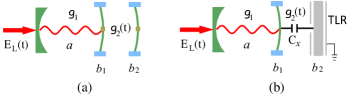
Figure 1: (Color online) Schematic representation of the system. An optical cavity mode $a$ driven by a two-tone laser $E_{L}(t)$ is coupled to an intermediate mechanical mode $b_{1}$ with single-photon optomechanical coupling strength $g_{1}$. $b_{1}$ is in turn coupled, with a time-dependent coupling strength $g_{2}(t)$, to (a) another mechanical oscillator, or alternatively to (b) a transmission line resonator $b_{2}$.

Applying the displacement transformation $a=\bar{a}_{+}e^{-iw_{1}t}+\bar{a}_{-}e^{iw_{1}t}+d$ to Eq. (4) in the strong driving case, we obtain the linearized Hamiltonian by discarding all nonlinear terms of the quantum fluctuations provided that the single-photon optomechanical coupling $g_{1}$ is small,

$$H_{lin}=H_{0}+H_{1}+H_{2},$$ (5)

with

$$H_{0}= \delta(d^{\dagger}d-b_{2}^{\dagger}b_{2}),$$ (6a)

$$H_{1}= g_{1}[(\bar{a}_{+}b_{1}d+\bar{a}_{-}b_{1}d^{\dagger})+(\bar{a}_{+}b_{1}d^{\dagger}$$

$$+\bar{a}_{-}b_{1}d)e^{-2iw_{1}t}]+h.c.,$$ (6b)

$$H_{2}= g_{2}^{A}\Big{\{}b_{1}b_{2}[1+e^{-2i(w_{1}+w_{2}+\delta)t}]$$

$$+b_{1}b_{2}^{\dagger}[e^{2i(w_{2}+\delta)t}+e^{-2iw_{1}t}]\Big{\}}$$

$$+g_{2}^{B}\Big{\{}b_{1}b_{2}[e^{-2i(w_{2}+\delta)t}+e^{-2iw_{1}t}]$$

$$+b_{1}b_{2}^{\dagger}[1+e^{-2i(w_{1}-w_{2}-\delta)t}]\Big{\}}+h.c.,$$ (6c)

where the classical cavity field amplitudes $\bar{a}_{\pm}$ are assumed to be real

$$\bar{a}_{\pm}=i\epsilon_{\pm}/(-\kappa/2-i\delta\pm iw_{1}),$$ (7)

and $\kappa$ is the cavity decay rate. If we set $g_{1}\bar{a}_{+}=g_{2}^{A}=G_{+}$, $g_{1}\bar{a}_{-}=g_{2}^{B}=G_{-}$, under the conditions $w_{1},w_{2},|w_{1}-w_{2}-\delta|\gg G_{\pm}$, all the non-resonant terms in the linearized Hamiltonian $H_{lin}$ can be effectively neglected under the rotating-wave approximation

$$H_{RWA}=\delta(\beta_{1}^{\dagger}\beta_{1}-\beta_{2}^{\dagger}\beta_{2})+[G(\beta_{1}^{\dagger}+\beta_{2}^{\dagger})b_{1}+h.c.],$$ (8)

where the Bogoliubove modes $\beta_{1}$ and $\beta_{2}$ are unitary transformations of $d$ and $b_{2}$, respectively

$$\beta_{1}= s(r)ds^{\dagger}(r)=d\cosh r+b_{2}^{\dagger}\sinh r,$$ (9a)

$$\beta_{2}= s(r)b_{2}s^{\dagger}(r)=b_{2}\cosh r+d^{\dagger}\sinh r.$$ (9b)

Here, $G=\sqrt{G_{-}^{2}-G_{+}^{2}}$ (we have assumed $G_{+}<G_{-}$ to ensure stability) and $s(r)=\exp[r(db_{2}-d^{\dagger}b_{2}^{\dagger})]$ is the two-mode squeezing operator with the squeezing parameter $r=\tanh^{-1}(G_{+}/G_{-})$. It’s clear from Eq. (9) that the joint ground state of $\beta_{1}$ and $\beta_{2}$ is the two-mode squeezed vacuum state of the cavity mode $d$ and the mechanical mode $b_{2}$. Introducing the sum mode and the difference mode of Bogoliubov modes

$$\beta_{sum}=(\beta_{1}+\beta_{2})/\sqrt{2},\ \beta_{diff}=(\beta_{1}-\beta_{2})/\sqrt{2},$$ (10)

then the Hamiltonian in Eq. (8) becomes

$$H_{RWA}=\delta\beta_{sum}^{\dagger}\beta_{diff}+\sqrt{2}G\beta_{sum}^{\dagger}b_{1}+h.c.,$$ (11)

which is similar to that of Ref. Woolley and Clerk (2014). Obviously, the sum mode $\beta_{sum}$ is coupled to both the intermediate mechanical mode $b_{1}$ and the difference mode $\beta_{diff}$ each via a beam-splitter-like interaction. Through the intermediate mechanical mode $b_{1}$ acting as an engineered reservoir, both the sum and difference modes, i.e., the two Bogoliubove modes $\beta_{1}$ and $\beta_{2}$, can be cooled to near ground state, generating two-mode squeezing between the cavity mode $d$ and the mechanical mode $b_{2}$.

III entanglement and purity

The quantum Langevin equations governing the dynamics of the linearized system can be written as

$$\dot{d}= i[H_{lin},d]-\frac{\kappa}{2}d+\sqrt{\kappa}d_{in},$$ (12a)

$$\dot{b}_{j}= i[H_{lin},b_{j}]-\frac{\gamma_{j}}{2}b_{j}+\sqrt{\gamma_{j}}b_{j,in},$$ (12b)

where $\gamma_{j}$ ($j=1,2$) is the damping rate for the $j$th mechanical oscillator, and $d_{in}$ and $b_{j,in}$ are independent zero mean vacuum input noise operators obeying the following correlation functions

$$<d_{in}(t)d_{in}^{\dagger}(t^{\prime})>= (\bar{n}_{d}+1)\delta(t-t^{\prime}),$$ (13a)

$$<d_{in}^{\dagger}(t)d_{in}(t^{\prime})>= \bar{n}_{d}\delta(t-t^{\prime}),$$ (13b)

$$<b_{j,in}(t)b_{j,in}^{\dagger}(t^{\prime})>= (\bar{n}_{j}+1)\delta(t-t^{\prime}),$$ (13c)

$$<b_{j,in}^{\dagger}(t)b_{j,in}(t^{\prime})>= \bar{n}_{j}\delta(t-t^{\prime})$$ (13d)

with $\bar{n}_{d}$ and $\bar{n}_{j}$ being equilibrium mean thermal occupancies of the cavity and the $j$th mechanical baths, respectively.

Introducing the position and momentum quadratures for the bosonic modes and their input noises

$$Q_{o}=(o+o^{\dagger})/\sqrt{2},\ P_{o}=(o-o^{\dagger})/(i\sqrt{2}),$$ (14)

with $o\in\{d,b_{1},b_{2},d_{in},b_{1,in},b_{2,in}\}$ and the vectors of all quadratures

$$R= [Q_{d},P_{d},Q_{b_{1}},P_{b_{1}},Q_{b_{2}},P_{b_{2}}]^{T},$$ (15a)

$$N= [\sqrt{\kappa}Q_{d_{in}},\sqrt{\kappa}P_{d_{in}},\sqrt{\gamma_{1}}Q_{b_{1,in}},$$

$$\sqrt{\gamma_{1}}P_{b_{1,in}},\sqrt{\gamma_{2}}Q_{b_{2,in}},\sqrt{\gamma_{2}}P_{b_{2,in}}]^{T},$$ (15b)

the linearized quantum Langevin equations (12) can be written in a compact form

$$\dot{R}=M(t)R+N.$$ (16)

Here, $M(t)$ is a $6\times 6$ time-dependent matrix

$$M(t)=\left({\begin{array}[]{*{20}{c}}-\kappa/2&\delta&Im(G_{1}+G_{2})&Re(G_{2}-G_{1})&0&0\\ -\delta&-\kappa/2&-Re(G_{2}+G_{1})&Im(G_{2}-G_{1})&0&0\\ Im(G_{1}-G_{2})&Re(G_{2}-G_{1})&-\gamma_{1}/2&0&Im(G_{3}+G_{4})&Re(G_{4}-G_{3})\\ -Re(G_{2}+G_{1})&-Im(G_{1}+G_{2})&0&-\gamma_{1}/2&-Re(G_{3}+G_{4})&Im(G_{4}-G_{3})\\ 0&0&Im(G_{3}-G_{4})&Re(G_{4}-G_{3})&-\gamma_{2}/2&-\delta\\ 0&0&-Re(G_{3}+G_{4})&-Im(G_{3}+G_{4})&\delta&-\gamma_{2}/2\end{array}}\right),$$ (23)

where $Re$ and $Im$ respectively denote the real and imaginary parts. $G_{1}\sim G_{4}$ are given by

$$G_{1}= G_{+}+G_{-}e^{2iw_{1}t},$$ (24a)

$$G_{2}= G_{-}+G_{+}e^{-2iw_{1}t},$$ (24b)

$$G_{3}= G_{+}[1+e^{2i(w_{1}+w_{2}+\delta)t}]$$

$$+G_{-}[e^{2i(w_{2}+\delta)t}+e^{2iw_{1}t}],$$ (24c)

$$G_{4}= G_{-}[1+e^{2i(w_{1}-w_{2}-\delta)t}]$$

$$+G_{+}[e^{-2i(w_{2}+\delta)t}+e^{2iw_{1}t}].$$ (24d)

Since the system is linearized, it remains Gaussian starting from an initial Gaussian state whose information-related properties can be fully described by the covariance matrix Adesso and Illuminati (2007); Weedbrook et al. (2012); Olivares and Paris (2012). For our three-mode bosonic system, the covariance matrix $\sigma$ is a $6\times 6$ matrix with components defined as

$$\sigma_{j,k}=<R_{j}R_{k}+R_{k}R_{j}>/2,$$ (25)

where $R_{k}$ is the $k$th component of the vector of quadratures $R$ in Eq. (15). From Eqs. (13), (15), and (16), we can derive a linear differential equation of the covariance matrix that is equivalent to the quantum Langevin equation (16) when only Gaussian states are relevant Mari and Eisert (2009),

$$\dot{\sigma}=M(t)\sigma+\sigma M(t)^{T}+D.$$ (26)

Here, $D$ is a diffusion matrix whose components are associated with the noise correlation functions (see Eq. (13))

$$D_{j,k}\delta(t-t^{\prime})=<N_{j}(t)N_{k}(t^{\prime})+N_{k}(t^{\prime})N_{j}(t)>/2.$$ (27)

$D$ is found to be diagonal,

$$D = {\rm{diag}}\{\kappa(2\bar{n}_{d}+1)/2,\kappa(2\bar{n}_{d}+1)/2,\gamma_{1}(2\bar{n}_{1}+1)/2,$$ (28)

$$\gamma_{1}(2\bar{n}_{1}+1)/2,\gamma_{2}(2\bar{n}_{2}+1)/2,\gamma_{2}(2\bar{n}_{2}+1)/2\}.$$

The general stability conditions of the linear differential equation (Eq. (16) or equally Eq. (26)) are determined by the corresponding homogeneous equation $\dot{R}=M(t)R$, which is fully characterized by the time-periodic coefficient matrix $M(t)$. Suppose that the period of the coefficient matrix $M(t)$ is $T>0$, i.e. $M(t)=M(t+T)$. Let $\Pi(t)$ be a principal matrix solution of the homogeneous equation. The eigenvalues $\lambda_{j}$ ($j=1,2,...,6$) of $\Lambda=\Pi^{-1}(0)\Pi(T)$ are called the characteristic multipliers or Floquet multipliers Teschl (2012), where $\Pi(T)$ can be obtained by numerical integration with the initial condition $\Pi(0)$. The solutions of Eq. (16) and Eq. (26) are stable if all Floquet multipliers satisfy $|\lambda_{j}|<1$. For the special case of a time-independent coefficient matrix $M=M(t=0)$ under the rotating-wave approximation, i.e. omitting all nonresonant terms in Eq. (5) (all time-dependent terms in Eq. (23)), the stability requirements can be readily inferred from the eigenvalues of the time-independent coefficient matrix $M$, i.e. all eigenvalues of $M$ having negative real parts. The stability conditions will be carefully checked in all simulations throughout this paper.

For two-mode Gaussian states of the cavity mode $d$ and the mechanical resonator $b_{2}$ of interest here, it is convenient to use the logarithmic negativity $E_{N}$ as a measurement of the entanglement Plenio (2005); Vidal and Werner (2002). $E_{N}$ can be computed from the reduced $4\times 4$ covariance matrix $\sigma_{r}$ for $d$ and $b_{2}$ whose components are just the terms associated with $d$ and $b_{2}$ only in the full covariance matrix $\sigma$. If we write $\sigma_{r}$ in the form

$$\sigma_{r}=\left({\begin{array}[]{*{20}{c}}V_{1}&V_{c}\\ V_{c}^{T}&V_{2}\end{array}}\right),$$ (31)

where $V_{1},V_{2}$, and $V_{c}$ are $2\times 2$ subblock matrices of $\sigma_{r}$, the logarithmic negativity $E_{N}$ is then given by

$$E_{N}=\max[0,-\ln(2\eta)],$$ (32)

with

$$\eta= 2^{-1/2}\{\Sigma-[\Sigma^{2}-4\det\sigma_{r}]^{1/2}\}^{1/2},$$ (33a)

$$\Sigma= \det V_{1}+\det V_{2}-2\det V_{c}.$$ (33b)

The purity of a two-mode Gaussian state described by a covariance matrix $\sigma_{r}$ is simply given by

$$\mu=1/(4\sqrt{\det\sigma_{r}}).$$ (34)

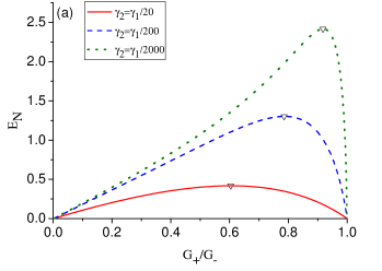
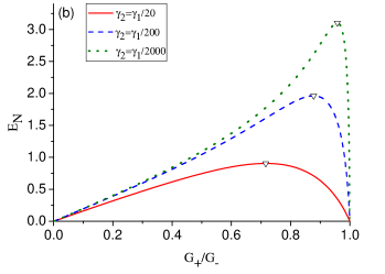
Figure 2: (Color online) Stationary cavity-mechanical entanglement $E_{N}$ versus the ratio of the effective couplings $G_{+}/G_{-}$ for different values of $\delta$. (a) $\delta=10\gamma_{1}$, (b) $\delta=5\gamma_{1}$, and (c) $\delta=\gamma_{1}$. The other parameters are: $G_{-}=2.5\gamma_{1}$, $\kappa=\gamma_{2}$, $\bar{n}_{1}=\bar{n}_{2}=\bar{n}_{d}=0$.

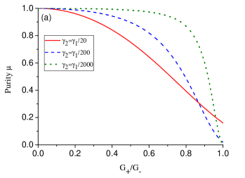
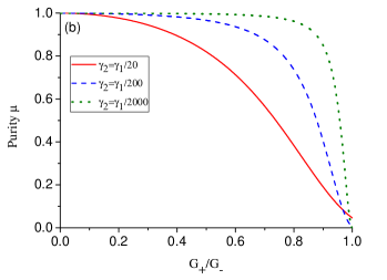
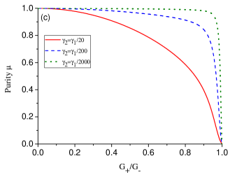
Figure 3: (Color online) Steady-state purity of the cavity mode $d$ and the mechanical mode $b_{2}$ against the ratio of the effective couplings $G_{+}/G_{-}$ for different values of $\delta$. (a) $\delta=10\gamma_{1}$, (b) $\delta=5\gamma_{1}$, and (c) $\delta=\gamma_{1}$. All other parameters are the same as those in Fig. 2.

We next study the steady-state entanglement ($\dot{\sigma}(t)=0$ in the stationary limit $t\gg 1/\kappa,\gamma_{1,2}$ if the system is stable) with the time-independent Hamiltonian in Eqs. (8) and  (11) under the rotating-wave approximation (by dropping all time-dependent terms in Eq. (23)). Fig. 2 displays the steady-state entanglement $E_{N}$ of the cavity mode $d$ and the mechanical mode $b_{2}$ as functions of the coupling asymmetry $G_{+}/G_{-}$ for different $\delta$ with zero bath occupations for all modes, where the downward triangle denotes the optimal value of each curve. Apparently, $E_{N}$ is a non-monotonic function of $G_{+}/G_{-}$ in any given set of parameters and takes a maximum for a specific $G_{+}/G_{-}$. The phenomenon is similar to that in Refs. Wang and Clerk (2013); Woolley and Clerk (2014); Chen et al. (2015), and it can be explained as follows. The relation $\tanh r=G_{+}/G_{-}$ indicates that the increase of the ratio $G_{+}/G_{-}$ can raise the squeezing parameter $r$, which is beneficial for enhancing the entanglement. But, from another point of view, the increase in $G_{+}/G_{-}$ (with $G_{-}$ fixed) accompanies the decline of effective coupling $G=\sqrt{G_{-}^{2}-G_{+}^{2}}$ between the sum mode $\beta_{sum}$ and the mechanical mode $b_{1}$ , which is harmful for the cooling effect and thus reduces the amount of entanglement. The best value is obtained when the two competing effects balance. In addition, we find that the smaller the ratio $\gamma_{2}/\gamma_{1}$, the lager the maximal entanglement $E_{N}$ and the optimal $G_{+}/G_{-}$ in each figure. Since the entanglement generation is largely based on cooling the Bogoliubov modes via the dissipative dynamics of the mechanical mode $b_{1}$, one would expect that a strong damping rate $\gamma_{1}$ of $b_{1}$ and simultaneously weak damping rates $\gamma_{2}$ of $b_{2}$ and $\kappa$ of $d$ should increase the peak entanglement $E_{N}$ (corresponding to bigger $G_{+}/G_{-}$). Comparing Figs. 2, 2 and 2 with different values of $\delta$, one can find that the achievable entanglement is also dependent on $\delta$, which is the effective coupling between the sum mode $\beta_{sum}$ and the difference mode $\beta_{diff}$ and induces the cooling process of $\beta_{diff}$.

Fig. 3 shows the purity as functions of the coupling asymmetry $G_{+}/G_{-}$. Clearly, we can observe that the purity is inversely correlated to $G_{+}/G_{-}$. If $\gamma_{2}$ is small enough compared to $\gamma_{1}$, one can keep the high purity ($\approx 1$) of the steady states over a wide range of $G_{+}/G_{-}$. However, in order to enhance the entanglement, one needs a larger squeezing parameter $r=\tanh^{-1}(G_{+}/G_{-})$ (i.e. larger $G_{+}/G_{-}$) which, on the other hand, weakens the effective coupling $G=\sqrt{G_{-}^{2}-G_{+}^{2}}$ and, hence, cripples the cooling process of Bogoliubov modes toward a pure ground state via the dissipation of $b_{1}$. For the sake of gaining a large amount of entanglement while retaining the relatively high purity of the entangled states, we can select proper detuning $\delta$ as shown in Figs. 4 and 5, where the downward triangles indicate the optimal values of the corresponding curves. Note that the chosen coupling asymmetry $G_{+}/G_{-}$ for each $\gamma_{2}$ is the value where $E_{N}$ takes the maximum in Fig. 2. Remarkably, one can find specific $\delta$ where both the entanglement and the purity take the local maximum. For example, when $\gamma_{2}=\gamma_{1}/2000,G_{+}/G_{-}=0.918,\delta\approx\gamma_{1}$, we have $E_{N}\approx 3.2$ and $\mu\approx 0.98$. In other words, our scheme allows the generation of highly pure and strongly entangled optomechanical states.

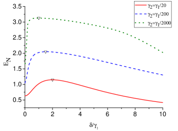
Figure 4: (Color online) Stationary cavity-mechanical entanglement $E_{N}$ versus the effective coupling $\delta$. The sets of parameters corresponding to different lines are $\gamma_{2}=\gamma_{1}/20,G_{+}/G_{-}=0.604$ (red solid); $\gamma_{2}=\gamma_{1}/200,G_{+}/G_{-}=0.786$ (blue dashed); and $\gamma_{2}=\gamma_{1}/2000,G_{+}/G_{-}=0.918$ (olive dotted). The other parameters are: $G_{-}=2.5\gamma_{1}$, $\kappa=\gamma_{2}$, $\bar{n}_{1}=\bar{n}_{2}=\bar{n}_{d}=0$.

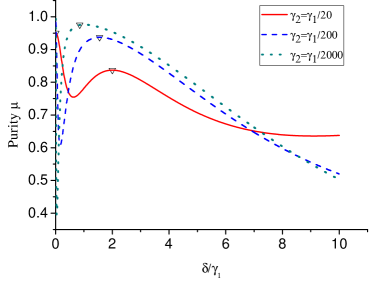
Figure 5: (Color online) Steady-state purity of the cavity mode $d$ and the mechanical mode $b_{2}$ versus the effective coupling $\delta$. All parameters are the same as those in Fig. 4.

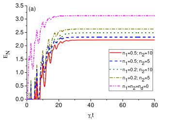
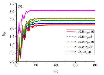
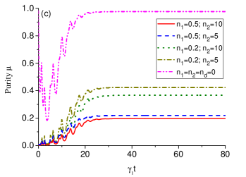
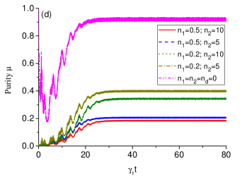
Figure 6: (Color online) The time evolution of the entanglement [(a) and (b)] and purity [(c) and (d)] of the quantum states of the cavity mode $d$ and mechanical mode $b_{2}$ with [(b) and (d)] and without [(a) and (c)] the non-resonant terms. The parameters are $G_{-}=2.5\gamma_{1}$, $G_{+}=0.918G_{-}$, $\kappa=\gamma_{2}=\gamma_{1}/2000$, $\delta=\gamma_{1}$, $\bar{n}_{2}=\bar{n}_{d}$, $\omega_{1}=10\gamma_{1}$, and $\omega_{2}=100\gamma_{1}$.

To find the optimal $\delta_{opt}$, one can recall the Hamiltonian under the rotating-wave approximation in Eq. (11). The sum mode $\beta_{sum}$ is simultaneously coupled to the difference mode $\beta_{diff}$ and the mechanical mode $b_{1}$ with beam-splitter-like coupling strengths $\delta$ and $\sqrt{2}G$ respectively. The coupling between $\beta_{sum}$ and $b_{1}$ induces the cooling process of $\beta_{sum}$, while the coupling between $\beta_{sum}$ and $\beta_{diff}$ is responsible for cooling the $\beta_{diff}$ mode. For a given (fixed) set of parameters $G_{+}$, $G_{-}$, on the one hand, if $\delta$ is too small (relative to $G=\sqrt{G_{-}^{2}-G_{+}^{2}}$), $\beta_{diff}$ can not be effectively cooled by $\beta_{sum}$. For example, when $\delta$ approaches 0, only the $\beta_{sum}$ mode can be cooled by $b_{1}$. On the other hand, if $\delta$ is too large, i.e., $\beta_{diff}$ and $\beta_{sum}$ are strongly coupled, the quanta are confined and swap rapidly between them. Hence, $\beta_{sum}$ can not be effectively cooled by $b_{1}$ in this case. For different sets of parameters $G_{+}$ and $G_{-}$, one would expect some moderate values of $\delta$ that correspond to maximum entanglement and purity. In fact, we have found that the optimal $\delta_{opt}$ is approximately equal to $G$ from Figs. 4 and 5, where $\delta_{opt}\approx G\approx 2\gamma_{1}$ for red solid lines, $\delta_{opt}\approx G\approx 1.5\gamma_{1}$ for blue dashed lines, and $\delta_{opt}\approx G\approx 0.99\gamma_{1}$ for olive dotted lines.

So far all of our discussions have been restricted to the rotating-wave approximation. To study the effects of non-resonant terms of the linearized Hamiltonian in Eq. (5), we plot in Fig. 6 the time evolution of the entanglement and purity with (Figs. 6 and 6) and without (Figs. 6 and 6) the non-resonant terms for some bath occupancies. We study the system dynamics by numerically solving the differential equation of the covariance matrix in Eq. (26) with the initial states of all modes assumed to be in thermal equilibrium with their local baths. When performing the numerical simulations, the effects of non-resonant terms are included by using the full time-dependent coefficient matrix $M(t)$ in Eq. (23) containing all time-dependent terms. We find that the non-resonant terms only induce small oscillations and do not significantly reduce the amount of steady-state entanglement and purity in the long-time limit, suggesting that the rotating-wave approximation is indeed valid.

IV conclusions

In summary, we have proposed an effective approach to generate pure and strong steady-state opto-mechanical entanglement (or optical-microwave entanglement) in a hybrid modulated three-mode optomechanical system. By applying a proper two-tone driving of the cavity and modulating coupling strength between two mechanical oscillators (or between a mechanical oscillator and a superconducting transmission line resonator), one can prepare the two target modes of the system in an entangled steady state. The proposal uses an intermediate mechanical mode acting as an engineered reservoir to effectively cool both Bogoliubov modes of the target modes to near their ground state via the beam-splitter-like interactions. Our approach allows the generation of a highly pure and strongly entangled steady state, by properly choosing not only the ratio of the effective optomechanical couplings but also the cavity-pump detuning.

References

- Fabre et al. (1994) C. Fabre, M. Pinard, S. Bourzeix, A. Heidmann, E. Giacobino, and S. Reynaud, Phys. Rev. A 49, 1337 (1994).
- Mancini and Tombesi (1994) S. Mancini and P. Tombesi, Phys. Rev. A 49, 4055 (1994).
- Jacobs et al. (1994) K. Jacobs, P. Tombesi, M. J. Collett, and D. F. Walls, Phys. Rev. A 49, 1961 (1994).
- Pinard et al. (1995) M. Pinard, C. Fabre, and A. Heidmann, Phys. Rev. A 51, 2443 (1995).
- Bose et al. (1997) S. Bose, K. Jacobs, and P. L. Knight, Phys. Rev. A 56, 4175 (1997).
- Mancini et al. (1997) S. Mancini, V. I. Man’ko, and P. Tombesi, Phys. Rev. A 55, 3042 (1997).
- Schwab and Roukes (2005) K. C. Schwab and M. L. Roukes, Phys. Today 58, 36 (2005).
- Cohadon et al. (1999) P. F. Cohadon, A. Heidmann, and M. Pinard, Phys. Rev. Lett. 83, 3174 (1999).
- Chen (2013) Y. Chen, J. Phys. B 46, 104001 (2013).
- Hammerer et al. (2009) K. Hammerer, M. Wallquist, C. Genes, M. Ludwig, F. Marquardt, P. Treutlein, P. Zoller, J. Ye, and H. J. Kimble, Phys. Rev. Lett. 103, 063005 (2009).
- Hammerer et al. (2010) K. Hammerer, A. S. Sørensen, and E. S. Polzik, Rev. Mod. Phys. 82, 1041 (2010).
- Chen et al. (2010) W. Chen, D. S. Goldbaum, M. Bhattacharya, and P. Meystre, Phys. Rev. A 81, 053833 (2010).
- Jing et al. (2011) H. Jing, D. S. Goldbaum, L. Buchmann, and P. Meystre, Phys. Rev. Lett. 106, 223601 (2011).
- O’Connell et al. (2010) A. D. O’Connell, M. Hofheinz, M. Ansmann, R. C. Bialczak, M. Lenander, E. Lucero, M. Neeley, D. Sank, H. Wang, M. Weides, J. Wenner, J. M. Martinis, and A. N. Cleland, Nature (London) 464, 697 (2010).
- Jiang et al. (2009) X. Jiang, Q. Lin, J. Rosenberg, K. Vahala, and O. Painter, Opt. Express 17, 20911 (2009).
- Wiederhecker et al. (2009) G. S. Wiederhecker, L. Chen, A. Gondarenko, and M. Lipson, Nature (London) 462, 633 (2009).
- Ma et al. (2007) R. Ma, A. Schliesser, P. Del’Haye, A. Dabirian, G. Anetsberger, and T. J. Kippenberg, Opt. Lett. 32, 2200 (2007).
- Park and Wang (2009) Y. S. Park and H. L. Wang, Nat. Phys. 5, 489 (2009).
- Thompson et al. (2008) J. D. Thompson, B. M. Zwickl, A. M. Jayich, F. Marquardt, S. M. Girvin, and J. G. E. Harris, Nature (London) 452, 72 (2008).
- Favero et al. (2009) I. Favero, S. Stapfner, D. Hunger, P. Paulitschke, J. Reichel, H. Lorenz, E. M. Weig, and K. Karrai, Opt. Express 17, 12813 (2009).
- Regal et al. (2008) C. A. Regal, J. D. Teufel, and K. W. Lehnert, Nat. Phys. 4, 555 (2008).
- Lee et al. (2010) K. H. Lee, T. G. McRae, G. I. Harris, J. Knittel, and W. P. Bowen, Phys. Rev. Lett. 104, 123604 (2010).
- Winger et al. (2011) M. Winger, T. D. Blasius, T. P. M. Alegre, A. H. Safavi-Naeini, S. Meenehan, J. Cohen, S. Stobbe, and O. Painter, Opt. Express 19, 24905 (2011).
- Barzanjeh et al. (2011) S. Barzanjeh, D. Vitali, P. Tombesi, and G. J. Milburn, Phys. Rev. A 84, 042342 (2011).
- Schmidt et al. (2012) M. Schmidt, M. Ludwig, and F. Marquardt, New J. Phys. 14, 125005 (2012).
- Mari and Eisert (2009) A. Mari and J. Eisert, Phys. Rev. Lett. 103, 213603 (2009).
- Mari and Eisert (2012) A. Mari and J. Eisert, New J. Phys. 14, 075014 (2012).
- Abdi and Hartmann (2015) M. Abdi and M. J. Hartmann, New J. Phys. 17, 013056 (2015).
- Li et al. (2015a) Z. Li, S.-l. Ma, and F.-l. Li, Phys. Rev. A 92, 023856 (2015a).
- Wang et al. (2016) M. Wang, X.-Y. Lü, Y.-D. Wang, J. Q. You, and Y. Wu, Phys. Rev. A 94, 053807 (2016).
- Chen et al. (2014) R.-X. Chen, L.-T. Shen, Z.-B. Yang, H.-Z. Wu, and S.-B. Zheng, Phys. Rev. A 89, 023843 (2014).
- Chen et al. (2017) R. X. Chen, C. G. Liao, and X. M. Lin, Sci. Rep. 7, 14497 (2017).
- Wang and Clerk (2013) Y.-D. Wang and A. A. Clerk, Phys. Rev. Lett. 110, 253601 (2013).
- Wang et al. (2015) Y.-D. Wang, S. Chesi, and A. A. Clerk, Phys. Rev. A 91, 013807 (2015).
- Tan et al. (2013) H. Tan, G. Li, and P. Meystre, Phys. Rev. A 87, 033829 (2013).
- Woolley and Clerk (2014) M. J. Woolley and A. A. Clerk, Phys. Rev. A 89, 063805 (2014).
- Yang et al. (2015) C.-J. Yang, J.-H. An, W. Yang, and Y. Li, Phys. Rev. A 92, 062311 (2015).
- Li et al. (2015b) J. Li, I. M. Haghighi, N. Malossi, S. Zippilli, and D. Vitali, New J. Phys. 17, 103037 (2015b).
- Qu and Agarwal (2014) K. Qu and G. S. Agarwal, New Journal of Physics 16, 113004 (2014).
- Chen et al. (2015) R.-X. Chen, L.-T. Shen, and S.-B. Zheng, Phys. Rev. A 91, 022326 (2015).
- Ockeloen-Korppi et al. (2017) C. F. Ockeloen-Korppi, E. Damskagg, J. M. Pirkkalainen, A. A. Clerk, F. Massel, M. J. Woolley, and M. A. Sillanpaa, arXiv:1711.01640 (2017).
- Vitali et al. (2007) D. Vitali, S. Gigan, A. Ferreira, H. R. Böhm, P. Tombesi, A. Guerreiro, V. Vedral, A. Zeilinger, and M. Aspelmeyer, Phys. Rev. Lett. 98, 030405 (2007).
- Paternostro et al. (2007) M. Paternostro, D. Vitali, S. Gigan, M. S. Kim, C. Brukner, J. Eisert, and M. Aspelmeyer, Phys. Rev. Lett. 99, 250401 (2007).
- Braunstein and Kimble (1998) S. L. Braunstein and H. J. Kimble, Phys. Rev. Lett. 80, 869 (1998).
- Adesso and Illuminati (2005) G. Adesso and F. Illuminati, Phys. Rev. Lett. 95, 150503 (2005).
- Okamoto et al. (2013) H. Okamoto, A. Gourgout, C.-Y. Chang, K. Onomitsu, I. Mahboob, E. Y. Chang, and H. Yamaguchi, Nat. Phys. 9, 480 (2013).
- Buks and Roukes (2002) E. Buks and M. L. Roukes, J. Microelectromech. Syst. 11, 802 (2002).
- Hensinger et al. (2005) W. K. Hensinger, D. W. Utami, H.-S. Goan, K. Schwab, C. Monroe, and G. J. Milburn, Phys. Rev. A 72, 041405 (2005).
- Zhang et al. (2012) J.-Q. Zhang, Y. Li, M. Feng, and Y. Xu, Phys. Rev. A 86, 053806 (2012).
- Ma et al. (2014) P.-C. Ma, J.-Q. Zhang, Y. Xiao, M. Feng, and Z.-M. Zhang, Phys. Rev. A 90, 043825 (2014).
- Adesso and Illuminati (2007) G. Adesso and F. Illuminati, J. Phys. A 40, 7821 (2007).
- Weedbrook et al. (2012) C. Weedbrook, S. Pirandola, R. García-Patrón, N. J. Cerf, T. C. Ralph, J. H. Shapiro, and S. Lloyd, Rev. Mod. Phys. 84, 621 (2012).
- Olivares and Paris (2012) S. Olivares and M. G. A. Paris, Eur. Phys. J. Special Topics 203, 185 (2012).
- Teschl (2012) G. Teschl, Ordinary differential equations and dynamical systems (Amer. Math. Soc., Providence, 2012).
- Plenio (2005) M. B. Plenio, Phys. Rev. Lett. 95, 090503 (2005).
- Vidal and Werner (2002) G. Vidal and R. F. Werner, Phys. Rev. A 65, 032314 (2002).