Low-Rank Matrix Approximations with
Flip-Flop Spectrum-Revealing QR Factorization

Abstract

We present Flip-Flop Spectrum-Revealing QR (Flip-Flop SRQR) factorization, a significantly faster and more reliable variant of the QLP factorization of Stewart, for low-rank matrix approximations. Flip-Flop SRQR uses SRQR factorization to initialize a partial column pivoted QR factorization and then compute a partial LQ factorization. As observed by Stewart in his original QLP work, Flip-Flop SRQR tracks the exact singular values with “considerable fidelity”. We develop singular value lower bounds and residual error upper bounds for Flip-Flop SRQR factorization. In situations where singular values of the input matrix decay relatively quickly, the low-rank approximation computed by SRQR is guaranteed to be as accurate as truncated SVD. We also perform a complexity analysis to show that for the same accuracy, Flip-Flop SRQR is faster than randomized subspace iteration for approximating the SVD, the standard method used in Matlab tensor toolbox. We also compare Flip-Flop SRQR with alternatives on two applications, tensor approximation and nuclear norm minimization, to demonstrate its efficiency and effectiveness.

Keywords: QR factorization, randomized algorithm, low-rank approximation, approximate SVD, higher-order SVD, nuclear norm minimization

AMS subject classifications. 15A18, 15A23, 65F99

1 Introduction

The singular value decomposition (SVD) of a matrix $A\in\mathbb{R}^{m\times n}$ is the factorization of $A$ into the product of three matrices $A=U\Sigma V^{T}$ where $U=\left(u_{1},\cdots,u_{m}\right)\in\mathbb{R}^{m\times m}$ and $V=\left(v_{1},\cdots,v_{n}\right)\in\mathbb{R}^{n\times n}$ are orthogonal singular vector matrices and $\Sigma\in\mathbb{R}^{m\times n}$ is a rectangular diagonal matrix with non-increasing non-negative singular values $\sigma_{i}\left(1\leq i\leq\min\left(m,n\right)\right)$ on the diagonal. The SVD has become a critical analytic tool in large data analysis and machine learning [1, 20, 51].

Let $\mbox{Diag}\left(x\right)$ denote the diagonal matrix with vector $x\in\mathbb{R}^{n}$ on its diagonal. For any $1\leq k\leq\min\left(m,n\right)$, the rank-$k$ truncated SVD of A is defined by

$$A_{k}\stackrel{{\scriptstyle def}}{{=}}\left(u_{1},\cdots,u_{k}\right)\mbox{Diag}\left(\sigma_{1},\cdots,\sigma_{k}\right)\left(v_{1},\cdots,v_{k}\right)^{T}.$$

The rank-$k$ truncated SVD turns out to be the best rank-$k$ approximation to $A$, as explained by Theorem 1.1.

Theorem 1.1.

(Eckart–Young–Mirsky Theorem [19, 26]).

$$\min_{rank\left(C\right)\leq k}\|A-C\|_{2} =\|A-A_{k}\|_{2}=\sigma_{k+1},$$

$$\min_{rank\left(C\right)\leq k}\|A-C\|_{F} =\|A-A_{k}\|_{F}=\sqrt{\sum_{j=k+1}^{\min\left(m,n\right)}\sigma_{j}^{2}},$$

where $\|\cdot\|_{2}$ and $\|\cdot\|_{F}$ denote the $l_{2}$ operator norm and the Frobenius norm respectively.

However, due to the prohibitive costs in computing the rank-$k$ truncated SVD, in practical applications one typically computes a rank-$k$ approximate SVD which satisfies some tolerance requirements [17, 27, 30, 40, 64]. Then rank-$k$ approximate SVD has been applied to many research areas including principal component analysis (PCA) [36, 56], web search models [37], information retrieval [4, 23], and face recognition [50, 68].

Among assorted SVD approximation algorithms, the pivoted QLP decomposition proposed by Stewart [64] is an effective and efficient one. The pivoted QLP decomposition is obtained by computing a QR factorization with column pivoting [6, 25] on $A$ to get an upper triangular factor $R$ and then computing an LQ factorization on $R$ to get a lower triangular factor $L$. Stewart’s key numerical observation is that the diagonal elements of $L$ track the singular values of $A$ with “considerable fidelity” no matter the matrix $A$. The pivoted QLP decomposition is extensively analyzed in Huckaby and Chan [34, 35]. More recently, Deursch and Gu developed a much more efficient variant of the pivoted QLP decomposition, TUXV, and demonstrated its remarkable quality as a low-rank approximation empirically without a rigid justification of TUXV’s success theoretically [18].

In this paper, we present Flip-Flop SRQR, a slightly different variant of TUXV of Deursch and Gu [18]. Like TUXV, Flip-Flop SRQR performs most of its work in computing a partial QR factorization using truncated randomized QRCP (TRQRCP) and a partial LQ factorization. Unlike TUXV, however, Flip-Flop SRQR also performs additional computations to ensure a spectrum-revealing QR factorization (SRQR) [74] before the partial LQ factorization.

We demonstrate the remarkable theoretical quality of this variant as a low-rank approximation, and its highly competitiveness with state-of-the-art low-rank approximation methods in real world applications in both low-rank tensor compression [13, 39, 58, 69] and nuclear norm minimization [7, 44, 48, 52, 65].

The rest of this paper is organized as follows: In Section 2 we introduce the TRQRCP algorithm, the spectrum-revealing QR factorization, low-rank tensor compression, and nuclear norm minimization. In Section 3, we introduce Flip-Flop SRQR and analyze its computational costs and low-rank approximation properties. In Section 4, we present numerical experimental results comparing Flip-Flop SRQR with state-of-the-art low-rank approximation methods.

2 Preliminaries and Background

2.1 Partial QRCP

Algorithm 1 Partial QRCP

Inputs:

Matrix $A\in\mathbb{R}^{m\times n}$. Target rank $k$.

Outputs:

Orthogonal matrix $Q\in\mathbb{R}^{m\times m}$.

Upper trapezoidal matrix $R\in\mathbb{R}^{m\times n}$.

Permutation matrix $\Pi\in\mathbb{R}^{n\times n}$ such that $A\Pi=QR$.

Algorithm:

Initialize $\Pi=I_{n}$. Compute column norms $r_{s}=\|A\left(1:m,s\right)\|_{2}~{}\left(1\leq s\leq n\right)$.

for $j=1:k$ do

   Find $i=\arg\max\limits_{j\leq s\leq n}r_{s}$. Exchange $r_{j}$ and $r_{i}$ columns in $A$ and $\Pi$.

   Form Householder reflection $Q_{j}$ from $A\left(j:m,j\right)$.

   Update trailing matrix $A\left(j:m,j:n\right)\leftarrow Q_{j}^{T}A\left(j:m,j:n\right)$.

   Update $r_{s}=\|A\left(j+1:m,s\right)\|_{2}~{}\left(j+1\leq s\leq n\right)$.

end for

$Q=Q_{1}Q_{2}\cdots Q_{k}$ is the product of all reflections. $R=$ upper trapezoidal part of $A$.

The QR factorization of a matrix $A\in\mathbb{R}^{m\times n}$ is $A=QR$ with orthogonal matrix $Q\in\mathbb{R}^{m\times m}$ and upper trapezoidal matrix $R\in\mathbb{R}^{m\times n}$, which can be computed by LAPACK [2] routine xGEQRF, where x stands for the matrix data type. The standard QR factorization is not suitable for some practical situations where either the matrix $A$ is rank deficient or only representative columns of $A$ are of interest. Usually the QR factorization with column pivoting (QRCP) is adequate for the aforementioned situations except a few rare examples such as the Kahan matrix [26]. Given a matrix $A\in\mathbb{R}^{m\times n}$, the QRCP of matrix $A$ has the form

$$A\Pi=QR,$$

where $\Pi\in\mathbb{R}^{n\times n}$ is a permutation matrix, $Q\in\mathbb{R}^{m\times m}$ is an orthogonal matrix, and $R\in\mathbb{R}^{m\times n}$ is an upper trapezoidal matrix. QRCP can be computed by LAPACK [2] routines xGEQPF and xGEQP3, where xGEQP3 is a more efficient blocked implementation of xGEQPF. For given target rank $k~{}\left(1\leq k\leq\min\left(m,n\right)\right)$, the partial QRCP factorization has a $2\times 2$ block form

$$A\Pi=Q\begin{pmatrix}R_{11}&R_{12}\\ &R_{22}\end{pmatrix}=\begin{pmatrix}Q_{1}&Q_{2}\end{pmatrix}\begin{pmatrix}R_{11}&R_{12}\\ &R_{22}\end{pmatrix},$$ (1)

where $R_{11}\in\mathbb{R}^{k\times k}$ is upper triangular. The details of partial QRCP are covered in Algorithm 1. The partial QRCP computes an approximate column subspace of $A$ spanned by the leading $k$ columns in $A\Pi$, up to the error term in $R_{22}$. Equivalently, (1) yields a low rank approximation

$$A\approx Q_{1}\begin{pmatrix}R_{11}&R_{12}\end{pmatrix}\Pi^{T},$$ (2)

with approximation quality closely related to the error term in $R_{22}$.

Algorithm 2 Truncated Randomized QRCP (TRQRCP)

Inputs:

Matrix $A\in\mathbb{R}^{m\times n}$. Target rank $k$. Block size $b$. Oversampling size $p\geq 0$.

Outputs:

Orthogonal matrix $Q\in\mathbb{R}^{m\times m}$.

Upper trapezoidal matrix $R\in\mathbb{R}^{k\times n}$.

Permutation matrix $\Pi\in\mathbb{R}^{n\times n}$ such that $A\Pi\approx Q\left(:,1:k\right)R$.

Algorithm:

Generate i.i.d. Gaussian random matrix $\Omega\in\mathcal{N}\left(0,1\right)^{\left(b+p\right)\times m}$.

Form the initial sample matrix $B=\Omega A$ and initialize $\Pi=I_{n}$.

for $j=1:b:k$ do

   $b=\min\left(k-j+1,b\right)$.

   Do partial QRCP on $B\left(:,j:n\right)$ to obtain $b$ pivots.

   Exchange corresponding columns in $A,~{}B,~{}\Pi$ and $W^{T}$.

   Do QR on $A\left(j:m,j:j+b-1\right)$ using WY formula without updating the trailing matrix.

   Update $B\left(:,j+b:n\right)$.

end for

$Q=Q_{1}Q_{2}\cdots Q_{\lceil k/b\rceil}$. $R=$ upper trapezoidal part of the submatrix $A\left(1:k,1:n\right)$.

The Randomized QRCP (RQRCP) algorithm [18, 74] is a more efficient variant of Algorithm 1. RQRCP generates a Gaussian random matrix $\Omega\in\mathcal{N}\left(0,1\right)^{(b+p)\times m}$ with $b+p\ll m$, where the entries of $\Omega$ are independently sampled from normal distribution, to compress $A$ into $B=\Omega A$ with much smaller row dimension. In practice, $b$ is the block size and $p$ is the oversampling size. RQRCP repeatedly runs partial QRCP on $B$ to obtain $b$ column pivots, applies them to the matrix $A$, and then computes QR without pivoting (QRNP) on $A$ and updates the remaining columns of $B$. RQRCP exits this process when it reaches the target rank $k$. QRCP and RQRCP choose pivots on $A$ and $B$ respectively. RQRCP is significantly faster than QRCP as $B$ has much smaller row dimension than $A$. It is shown in [74] that RQRCP is as reliable as QRCP up to failure probabilities that decay exponentially with respect to the oversampling size $p$.

Since the trailing matrix of $A$ is usually not required for low-rank matrix approximations (see (2)), the TRQRCP (truncated RQRCP) algorithm of [18] re-organizes the computations in RQRCP to directly compute the approximation (2) without explicitly computing the trailing matrix $R_{22}$. For more details, both RQRCP and TRQRCP are based on the $WY$ representation of the Householder transformations [5, 53, 59]:

$$Q=Q_{1}Q_{2}\cdots Q_{k}=I-YTY^{T},$$

where $T\in\mathbb{R}^{k\times k}$ is an upper triangular matrix and $Y\in\mathbb{R}^{m\times k}$ is a trapezoidal matrix consisting of $k$ consecutive Householder vectors. Let $W^{T}\stackrel{{\scriptstyle def}}{{=}}T^{T}Y^{T}A$, then the trailing matrix update formula becomes $Q^{T}A=A-YW^{T}$. The main difference between RQRCP and TRQRCP is that while RQRCP computes the whole trailing matrix update, TRQRCP only computes the part of the update that affects the approximation (2). More discussions about RQRCP and TRQRCP can be found in [18]. The main steps of TRQRCP are briefly described in Algorithm 2.

With TRQRCP, the TUXV algorithm (Algorithm 7 in [18]) computes a low-rank approximation with the QLP factorization at a greatly accelerated speed, by computing a partial QR factorization with column pivoting, followed with a partial LQ factorization.

2.2 Spectrum-revealing QR Factorization

Algorithm 3 TUXV Algorithm

Inputs:

Matrix $A\in\mathbb{R}^{m\times n}$. Target rank $k$. Block size $b$. Oversampling size $p\geq 0$.

Outputs:

Column orthonormal matrices $U\in\mathbb{R}^{m\times k},~{}V\in\mathbb{R}^{n\times k}$, and upper triangular matrix $R\in\mathbb{R}^{k\times k}$ such that $A\approx URV^{T}$.

Algorithm:

Do TRQRCP on $A$ to obtain $Q\in\mathbb{R}^{m\times k},~{}R\in\mathbb{R}^{k\times n}$, and $\Pi\in\mathbb{R}^{n\times n}$.

$R=R\Pi^{T}$ and do LQ factorization, i.e., $[V,R]=qr(R^{T},0)$.

Compute $Z=AV$ and do QR factorization, i.e., $[U,R]=qr(Z,0)$.

Although both RQRCP and TRQRCP are very effective practical tools for low-rank matrix approximations, they are not known to provide reliable low-rank matrix approximations due to their underlying greediness in column norm based pivoting strategy. To solve this potential problem of column based QR factorization, Gu and Eisenstat [28] proposed an efficient way to perform additional column interchanges to enhance the quality of the leading $k$ columns in $A\Pi$ as a basis for the approximate column subspace. More recently, a more efficient and effective method, spectrum-revealing QR factorization (SRQR), was introduced and analyzed in [74] to compute the low-rank approximation (2). The concept of spectrum-revealing, first introduced in [73], emphasizes the utilization of partial QR factorization (2) as a low-rank matrix approximation, as opposed to the more traditional rank-revealing factorization, which emphasizes the utility of the partial QR factorization (1) as a tool for numerical rank determination. SRQR algorithm is described in Algorithm 4. SRQR initializes a partial QR factorization using RQRCP or TRQRCP and then verifies an SRQR condition. If the SRQR condition fails, it will perform a pair-wise swap between a pair of leading column (one of first $k$ columns of $A\Pi$) and trailing column (one of the remaining columns). The SRQR algorithm will always run to completion with a high-quality low-rank matrix approximation (2). For real data matrices that usually have fast decaying singular-value spectrum, this approximation is often as good as the truncated SVD. The SRQR algorithm of [74] explicitly updates the partial QR factorization (1) while swapping columns, but the SRQR algorithm can actually avoid any explicit computations on the trailing matrix $R_{22}$ using TRQRCP instead of RQRCP to obtain exactly the same partial QR initialization. Below we outline the SRQR algorithm.

In (1), let

$$\widetilde{R}\stackrel{{\scriptstyle def}}{{=}}\begin{pmatrix}R_{11}&a\\ &\alpha\end{pmatrix}$$ (3)

be the leading $\left(l+1\right)\times\left(l+1\right)$ submatrix of $R$. We define

$$g_{1}\stackrel{{\scriptstyle def}}{{=}}\frac{\|R_{22}\|_{1,2}}{|\alpha|}\qquad\mbox{and}\qquad g_{2}\stackrel{{\scriptstyle def}}{{=}}|\alpha|\left\|\widetilde{R}^{-T}\right\|_{1,2},$$ (4)

where $\|X\|_{1,2}$ is the largest column $2$-norm of $X$ for any given $X$. In [74], the authors proved approximation quality bounds involving $g_{1},g_{2}$ for the low-rank approximation computed by RQRCP or TRQRCP. RQRCP or TRQRCP will provide a good low-rank matrix approximation if $g_{1}$ and $g_{2}$ are $O(1)$. The authors also proved that $g_{1}\leq\sqrt{\frac{1+\varepsilon}{1-\varepsilon}}$ and $g_{2}\leq\frac{\sqrt{2(1+\varepsilon)}}{1-\varepsilon}\left(1+\sqrt{\frac{1+\varepsilon}{1-\varepsilon}}\right)^{l-1}$ for RQRCP or TRQRCP, where $0<\varepsilon<1$ is a user-defined parameter which guides the choice of the oversampling size $p$. For reasonably chosen $\varepsilon$ like $\varepsilon=\frac{1}{2}$, $g_{1}$ is a small constant while $g_{2}$ can potentially be a extremely large number, which can lead to poor low-rank approximation quality. To avoid the potential exponential explosion of $g_{2}$, the SRQR algorithm (Algorithm 4) proposed in [74] uses a pair-wise swapping strategy to guarantee that $g_{2}$ is below some user defined tolerance $g>1$ which is usually chosen to be a small number greater than one, like $2.0$.

Algorithm 4 Spectrum-revealing QR Factorization (SRQR)

Inputs:

Matrix $A\in\mathbb{R}^{m\times n}$. Target rank $k$. Block size $b$. Oversampling size $p\geq 0$.

Integer $l\geq k$. Tolerance $g>1$ for $g_{2}$.

Outputs:

Orthogonal matrix $Q\in\mathbb{R}^{m\times m}$ formed by the first $k$ reflectors.

Upper trapezoidal matrix $R\in\mathbb{R}^{k\times n}$.

Permutation matrix $\Pi\in\mathbb{R}^{n\times n}$ such that $A\Pi\approx Q\left(:,1:k\right)R$.

Algorithm:  

Compute $Q,R,\Pi$ with RQRCP or TRQRCP to $l$ steps.

Compute squared 2-norm of the columns of $B(:,l+1:n):\widehat{r}_{i}\;(l+1\leq i\leq n)$, where $B$ is a random projection of $A$ computed by RQRCP or TRQRCP.

Approximate squared 2-norm of the columns of $A(l+1:m,l+1:n):r_{i}=\widehat{r}_{i}/(b+p)\;(l+1\leq i\leq n)$.

$\imath={\bf argmax}_{l+1\leq i\leq n}\{r_{i}\}$.

Swap $\imath$-th and $(l+1)$-st columns of $A,\Pi,r$.

One-step QR factorization of $A(l+1:m,l+1:n)$.

$\left|\alpha\right|=R_{l+1,l+1}$.

$r_{i}=r_{i}-A(l+1,i)^{2}\;(l+2\leq i\leq n)$.

Generate a random matrix $\Omega\in\mathcal{N}(0,1)^{d\times(l+1)}\;(d\ll l)$.

Compute $g_{2}=\left|\alpha\right|\left\|\widetilde{R}^{-T}\right\|_{1,2}\approx\frac{\left|\alpha\right|}{\sqrt{d}}\left\|\Omega\widetilde{R}^{-T}\right\|_{1,2}$.

while $g_{2}>g$ do

   $\imath={\bf argmax}_{1\leq i\leq l+1}\{i\text{th column norm of }\Omega\widetilde{R}^{-T}\}$.

   Swap $\imath$-th and $(l+1)$-st columns of $A$ and $\Pi$ in a Round Robin rotation.

   Givens-rotate $R$ back into upper-trapezoidal form.

   $r_{l+1}=R_{l+1,l+1}^{2}$, $r_{i}=r_{i}+A(l+1,i)^{2}\;(l+2\leq i\leq n)$.

   $\imath={\bf argmax}_{l+1\leq i\leq n}\{r_{i}\}$.

   Swap $\imath$-th and $(l+1)$-st columns of $A,\Pi,r$.

   One-step QR factorization of $A(l+1:m,l+1:n)$.

   $\left|\alpha\right|=R_{l+1,l+1}$.

   $r_{i}=r_{i}-A(l+1,i)^{2}\;(l+2\leq i\leq n)$.

   Generate a random matrix $\Omega\in\mathcal{N}(0,1)^{d\times(l+1)}(d\ll l)$ .

   Compute $g_{2}=\left|\alpha\right|\left\|\widetilde{R}^{-T}\right\|_{1,2}\approx\frac{\left|\alpha\right|}{\sqrt{d}}\left\|\Omega\widetilde{R}^{-T}\right\|_{1,2}$.

end while

2.3 Tensor Approximation

In this section we review some basic notations and concepts involving tensors. A more detailed discussion of the properties and applications of tensors can be found in the review [39]. A tensor is a $d$-dimensional array of numbers denoted by script notation $\mathcal{X}\in\mathbb{R}^{I_{1}\times\cdots\times I_{d}}$ with entries given by

$$x_{j_{1},\dots,j_{d}},\quad 1\leq j_{1}\leq I_{1},\dots,1\leq j_{d}\leq I_{d}.$$

We use the matrix $X_{\left(n\right)}\in\mathbb{R}^{I_{n}\times\left(\Pi_{j\neq n}I_{j}\right)}$ to denote the $n$th mode unfolding of the tensor $\mathcal{X}$. Since this tensor has $d$ dimensions, there are altogether $d$-possibilities for unfolding. The $n$-mode product of a tensor $\mathcal{X}\in\mathbb{R}^{I_{1}\times\cdots\times I_{d}}$ with a matrix $U\in\mathbb{R}^{k\times I_{n}}$ results in a tensor $\mathcal{Y}\in\mathbb{R}^{I_{1}\times\cdots\times I_{n-1}\times k\times I_{n+1}\times\cdots\times I_{d}}$ such that

$$y_{j_{1},\dots,j_{n-1},j,j_{n+1},\dots,j_{d}}=\left(\mathcal{X}\times_{n}U\right)_{j_{1},\dots,j_{n-1},j,j_{n+1},\dots,j_{d}}=\sum_{j_{n}=1}^{I_{n}}x_{j_{1},\dots,j_{d}}u_{j,j_{n}}.$$

Alternatively it can be expressed conveniently in terms of unfolded tensors:

$$\mathcal{Y}=\mathcal{X}\times_{n}U\Leftrightarrow Y_{\left(n\right)}=UX_{\left(n\right)},.$$

Decompositions of higher-order tensors have applications in signal processing [12, 61, 15], numerical linear algebra [13, 38, 75], computer vision [70, 60, 72], etc. Two particular tensor decompositions can be considered as higher-order extensions of the matrix SVD: CANDECOMP/PARAFAC (CP) [10, 31] decomposes a tensor as a sum of rank-one tensors, and the Tucker decomposition [67] is a higher-order form of principal component analysis. Given the definitions of mode products and unfolding of tensors, we can define the higher-order SVD (HOSVD) algorithm for producing a rank $\left(k_{1},\dots,k_{d}\right)$ approximation to the tensor based on the Tucker decomposition format. The HOSVD algorithm [13, 39] returns a core tensor $\mathcal{G}\in\mathbb{R}^{k_{1}\times\cdots\times k_{d}}$ and a set of unitary matrices $U_{j}\in\mathbb{R}^{I_{j}\times k_{j}}$ for $j=1,\dots,d$ such that

$$\mathcal{X}\approx\mathcal{G}\times_{1}U_{1}\cdots\times_{d}U_{d},$$

where the right-hand side is called a Tucker decomposition. However, a straightforward generalization to higher-order ($d\geq 3$) tensors of the matrix Eckart–Young–Mirsky Theorem is not possible [14]; in fact, the best low-rank approximation is an ill-posed problem [16]. The HOSVD algorithm is outlined in Algorithm 5.

Algorithm 5 HOSVD

Inputs:

Tensor $\mathcal{X}\in\mathbb{R}^{I_{1}\times\cdots\times I_{d}}$ and desired rank $\left(k_{1},\dots,k_{d}\right)$.

Outputs:

Tucker decomposition $\left[\mathcal{G};U_{1},\cdots,U_{d}\right]$.

Algorithm:

for $j=1:d$ do

   Compute $k_{j}$ left singular vectors $U_{j}\in\mathbb{R}^{I_{j}\times k_{j}}$ of unfolding $X_{\left(j\right)}$.

end for

Compute core tensor $\mathcal{G}\in\mathbb{R}^{k_{1}\times\cdots\times k_{d}}$ as

$$\mathcal{G}\stackrel{{\scriptstyle def}}{{=}}\mathcal{X}\times_{1}U_{1}^{T}\times_{2}\cdots\times_{d}U_{d}^{T}.$$

Since HOSVD can be prohibitive for large-scale problems, there has been a lot of literature to improve the efficiency of HOSVD computations without a noticeable deterioration in quality. One strategy for truncating the HOSVD, sequentially truncated HOSVD (ST-HOSVD) algorithm, was proposed in [3] and studied by [69]. As was shown by [69], ST-HOSVD retains several of the favorable properties of HOSVD while significantly reducing the computational cost and memory consumption. The ST-HOSVD is outlined in Algorithm 6.

Algorithm 6 ST-HOSVD

Inputs:

Tensor $\mathcal{X}\in\mathbb{R}^{I_{1}\times\cdots\times I_{d}}$, desired rank $\left(k_{1},\dots,k_{d}\right)$, and processing order $p=\left(p_{1},\cdots,p_{d}\right)$.

Outputs:

Tucker decomposition $\left[\mathcal{G};U_{1},\cdots,U_{d}\right]$.

Algorithm:

Define tensor $\mathcal{G}\leftarrow\mathcal{X}$.

for $j=1:d$ do

   $r=p_{j}$.

   Compute exact or approximate rank $k_{r}$ SVD of the tensor unfolding $G_{\left(r\right)}\approx\widehat{U}_{r}\widehat{\Sigma}_{r}\widehat{V}_{r}^{T}$.

   $U_{r}\leftarrow\widehat{U}_{r}$.

   Update $G_{\left(r\right)}\leftarrow\widehat{\Sigma}_{r}\widehat{V}_{r}^{T}$, i.e., applying $\widehat{U}_{r}^{T}$ to $\mathcal{G}$.

end for

Unlike HOSVD, where the number of entries in tensor unfolding $X_{\left(j\right)}$ remains the same after each loop, the number of entries in $G_{\left(p_{j}\right)}$ decreases as $j$ increases in ST-HOSVD. In ST-HOSVD, one key step is to compute exact or approximate rank-$k_{r}$ SVD of the tensor unfolding. Well known efficient ways to compute an exact low-rank SVD include Krylov subspace methods [43]. There are also efficient randomized algorithms to find an approximate low-rank SVD [30]. In Matlab tensorlab toolbox [71], the most efficient method, MLSVD_RSI, is essentially ST-HOSVD with randomized subspace iteration to find approximate SVD of tensor unfolding.

2.4 Nuclear Norm Minimization

Matrix rank minimization problem appears ubiquitously in many fields such as Euclidean embedding [22, 45], control [21, 49, 54], collaborative filtering [9, 55, 63], system identification [46, 47], etc. Matrix rank minimization problem has the following form:

$$\min_{X\in\mathcal{C}}\;\;\mbox{rank}\left(X\right)$$

where $X\in\mathbb{R}^{m\times n}$ is the decision variable, and $\mathcal{C}$ is a convex set. In general, this problem is NP-hard due to the combinatorial nature of the function $\mbox{rank}\left(\cdot\right)$. To obtain a convex and more computationally tractable problem, $\mbox{rank}\left(X\right)$ is replaced by its convex envelope. In [21], authors proved that the nuclear norm $\|X\|_{*}$ is the convex envelope of $\mbox{rank}\left(X\right)$ on the set $\{X\in\mathbb{R}^{m\times n}:~{}\|X\|_{2}\leq 1\}$. The nuclear norm of a matrix $X\in\mathbb{R}^{m\times n}$ is defined as

$$\|X\|_{*}\stackrel{{\scriptstyle def}}{{=}}\sum_{i=1}^{q}\sigma_{i}\left(X\right),$$

where $q=\mbox{rank}\left(X\right)$ and $\sigma_{i}\left(X\right)$’s are the singular values of $X$.

In many applications, the regularized form of nuclear norm minimization problem is considered:

$$\min_{X\in\mathbb{R}^{m\times n}}f\left(X\right)+\tau\|X\|_{*}$$

where $\tau>0$ is a regularization parameter. The choice of function $f\left(\cdot\right)$ is situational: $f\left(X\right)=\|M-X\|_{1}$ in robust principal component analysis (robust PCA) [8], $f\left(X\right)=\|\pi_{\Omega}\left(M\right)-\pi_{\Omega}\left(X\right)||_{F}^{2}$ in matrix completion [7], $f\left(X\right)=\frac{1}{2}\|AX-B\|_{F}^{2}$ in multi-class learning and multivariate regression [48], where $M$ is the measured data, $\|\cdot\|_{1}$ denotes the $l_{1}$ norm, and $\pi_{\Omega}\left(\cdot\right)$ is an orthogonal projection onto the span of matrices vanishing outside of $\Omega$ so that $\left[\pi_{\Omega}\left(X\right)\right]_{i,j}=X_{ij}$ if $\left(i,j\right)\in\Omega$ and zero otherwise.

Many researchers have devoted themselves to solving the above nuclear norm minimization problem and plenty of algorithms have been proposed, including, singular value thresholding (SVT) [7], fixed point continuous (FPC) [48], accelerated proximal gradient (APG) [65], augmented Lagrange multiplier (ALM) [44]. The most expensive part of these algorithms is in the computation of the truncated SVD. Inexact augmented Lagrange multiplier (IALM) [44] has been proved to be one of the most accurate and efficient among them. We now describe IALM for robust PCA and matrix completion problems.

Robust PCA problem can be formalized as a minimization problem of sum of nuclear norm and scaled matrix $l_{1}$-norm (sum of matrix entries in absolute value):

$$\min\|X\|_{*}+\lambda\|E\|_{1},\qquad\mbox{subject to}\qquad M=X+E,$$ (5)

where $M$ is measured matrix, $X$ has low-rank, $E$ is a error matrix and sufficiently sparse, and $\lambda$ is a positive weighting parameter. Algorithm 7 describes the details of IALM method to solve robust PCA [44] problem, where $\|\cdot\|_{M}$ denotes the maximum absolute value of the matrix entries, and $\mathcal{S}_{\omega}\left(x\right)=\mbox{sgn}\left(x\right)\cdot\max\left(|x|-\omega,0\right)$ is the soft shrinkage operator [29] where $x\in\mathbb{R}^{n}$ and $\omega>0$.

Algorithm 7 Robust PCA Using IALM

Inputs:

Measured matrix $M\in\mathbb{R}^{m\times n}$, positive number $\lambda,~{}\mu_{0},~{}\overline{\mu}$, tolerance $tol$, $\rho>1$.

Outputs:

Matrix pair $\left(X_{k},E_{k}\right)$.

Algorithm:

$k=0$; $J\left(M\right)=\max\left(\|M\|_{2},\|M\|_{M}\right);~{}Y_{0}=M/J\left(M\right)$; $E_{0}=0$;

while not converged do

   $\mathbf{\left(U,\Sigma,V\right)=\mbox{\bf svd}\left(M-E_{k}+\mu_{k}^{-1}Y_{k}\right)}$;

   $X_{k+1}=U\mathcal{S}_{\mu_{k}^{-1}}\left(\Sigma\right)V^{T}$;

   $E_{k+1}=\mathcal{S}_{\lambda\mu_{k}^{-1}}\left(M-X_{k+1}+\mu_{k}^{-1}Y_{k}\right)$;

   $Y_{k+1}=Y_{k}+\mu_{k}\left(M-X_{k+1}-E_{k+1}\right)$;

   Update $\mu_{k+1}=\min\left(\rho\mu_{k},\overline{\mu}\right)$;

   $k=k+1$;

   if $\|M-X_{k}-E_{k}\|_{F}/\|M\|_{F}<tol$ then

      Break;

   end if

end while

Matrix completion problem [9, 44] can be written in the form:

$$\min_{X\in\mathbb{R}^{m\times n}}\|X\|_{*}\qquad\mbox{subject to}\qquad X+E=M,\quad\pi_{\Omega}\left(E\right)=0,$$ (6)

where $\pi_{\Omega}:~{}\mathbb{R}^{m\times n}\rightarrow\mathbb{R}^{m\times n}$ is an orthogonal projection that keeps the entries in $\Omega$ unchanged and sets those outside $\Omega$ zeros. In [44], authors applied IALM method on the matrix completion problem. We describe this method in Algorithm 8, where $\overline{\Omega}$ is the complement of $\Omega$.

Algorithm 8 Matrix Completion Using IALM

Inputs:

Sampled set $\Omega$, sampled entries $\pi_{\Omega}\left(M\right)$, positive number $\lambda,~{}\mu_{0},~{}\overline{\mu}$, tolerance $tol$, $\rho>1$.

Outputs:

Matrix pair $\left(X_{k},E_{k}\right)$.

Algorithm:

$k=0$; $Y_{0}=0$; $E_{0}=0$;

while not converged do

   $\mathbf{\left(U,\Sigma,V\right)=\mbox{\bf svd}\left(M-E_{k}+\mu_{k}^{-1}Y_{k}\right)}$;

   $X_{k+1}=U\mathcal{S}_{\mu_{k}^{-1}}\left(\Sigma\right)V^{T}$;

   $E_{k+1}=\pi_{\overline{\Omega}}\left(M-X_{k+1}+\mu_{k}^{-1}Y_{k}\right)$;

   $Y_{k+1}=Y_{k}+\mu_{k}\left(M-X_{k+1}-E_{k+1}\right)$;

   Update $\mu_{k+1}=\min\left(\rho\mu_{k},\overline{\mu}\right)$;

   $k=k+1$;

   if $\|M-X_{k}-E_{k}\|_{F}/\|M\|_{F}<tol$ then

      Break;

   end if

end while

3 Flip-Flop SRQR Factorization

3.1 Flip-Flop SRQR Factorization

In this section, we introduce our Flip-Flop SRQR factorization, a slightly different from TUXV (Algorithm 3), to compute SVD approximation based on QLP factorization. Given integer $l\geq k$, we run SRQR (the version without computing the trailing matrix) to $l$ steps on $A$,

$$A\Pi=QR=Q\left(\begin{array}[]{cc}R_{11}&R_{12}\\ &R_{22}\end{array}\right),$$ (7)

where $R_{11}\in\mathbb{R}^{l\times l}$ is upper triangular; $R_{12}\in\mathbb{R}^{l\times\left(n-l\right)}$; and $R_{22}\in\mathbb{R}^{\left(m-l\right)\times\left(n-l\right)}$. Then we run partial QRNP to $l$ steps on $R^{T}$,

$$R^{T}=\left(\begin{array}[]{cc}R_{11}^{T}&\\ R_{12}^{T}&R_{22}^{T}\end{array}\right)=\widehat{Q}\left(\begin{array}[]{cc}\widehat{R}_{11}&\widehat{R}_{12}\\ &\widehat{R}_{22}\end{array}\right)\approx\widehat{Q}_{1}\left(\begin{array}[]{cc}\widehat{R}_{11}&\widehat{R}_{12}\end{array}\right),$$ (8)

where $\widehat{Q}=\left(\begin{array}[]{cc}\widehat{Q}_{1}&\widehat{Q}_{2}\end{array}\right)$ with $\widehat{Q}_{1}\in\mathbb{R}^{n\times l}$. Therefore, combing the fact that $A\Pi\widehat{Q}_{1}=Q\begin{pmatrix}\widehat{R}_{11}&\widehat{R}_{12}\end{pmatrix}^{T}$, we can approximate matrix $A$ by

$$A=QR\Pi^{T}=Q\left(R^{T}\right)^{T}\Pi^{T}\approx Q\left(\begin{array}[]{c}\widehat{R}_{11}^{T}\\ \widehat{R}_{12}^{T}\end{array}\right)\widehat{Q}_{1}^{T}\Pi^{T}=A\left(\Pi\widehat{Q}_{1}\right)\left(\Pi\widehat{Q}_{1}\right)^{T}.$$ (9)

We denote the rank-$k$ truncated SVD of $A\Pi\widehat{Q}_{1}$ by $\widetilde{U}_{k}\Sigma_{k}\widetilde{V}_{k}^{T}$. Let $U_{k}=\widetilde{U}_{k},~{}V_{k}=\Pi\widehat{Q}_{1}\widetilde{V}_{k}$, then using (9), a rank-$k$ approximate SVD of $A$ is obtained:

$$A\approx U_{k}\Sigma_{k}V_{k}^{T},$$ (10)

where $U_{k}\in\mathbb{R}^{m\times k},~{}V_{k}\in\mathbb{R}^{n\times k}$ are column orthonormal; and $\Sigma_{k}=\mbox{Diag}\left(\sigma_{1},\cdots,\sigma_{k}\right)$ with $\sigma_{i}$’s are the leading $k$ singular values of $A\Pi\widehat{Q}_{1}$. The Flip-Flop SRQR factorization is outlined in Algorithm 9.

Algorithm 9 Flip-Flop Spectrum-Revealing QR Factorization

Inputs:

Matrix $A\in\mathbb{R}^{m\times n}$. Target rank $k$. Block size $b$. Oversampling size $p\geq 0$.

Integer $l\geq k$. Tolerance $g>1$ for $g_{2}$.

Outputs:

$U\in\mathbb{R}^{m\times k}$ contains the approximate top $k$ left singular vectors of $A$.

$\Sigma\in\mathbb{R}^{k\times k}$ contains the approximate top $k$ singular values of $A$.

$V\in\mathbb{R}^{n\times k}$ contains the approximate top $k$ right singular vectors of $A$.

Algorithm:

Run SRQR on $A$ to $l$ steps to obtain $\left(R_{11},R_{12}\right)$.

Run QRNP on $\left(R_{11},R_{12}\right)^{T}$ to obtain $\widehat{Q}_{1}$, represented by a sequence of Householder vectors.

$tmp=A\Pi\widehat{Q}_{1}$.

$[U_{tmp},\Sigma_{tmp},V_{tmp}]=svd\left(tmp\right)$.

$U=U_{tmp}\left(:,1:,k\right),\Sigma=\Sigma_{tmp}\left(1:k,1:k\right),V=\Pi\widehat{Q}_{1}V_{tmp}\left(:,1:k\right)$.

3.2 Complexity Analysis

In this section, we do complexity analysis of Flip-Flop SRQR. Since approximate SVD only makes sense when target rank $k$ is small, we assume $k\leq l\ll\min\left(m,n\right)$. The complexity analysis of Flip-Flop SRQR is as follows:

1. The cost of doing SRQR with TRQRCP on $A$ is $2mnl+2(b+p)mn+(m+n)l^{2}$.

2. The cost of QR factorization on $\left(R_{11},R_{12}\right)^{T}$ and forming $\widehat{Q}_{1}$ is $2nl^{2}-\frac{2}{3}l^{3}$.

3. The cost of computing $tmp=A\Pi\widehat{Q}_{1}$ is $2mnl$.

4. The cost of computing $[U,\sim,\sim]=svd\left(tmp\right)$ is $O(ml^{2})$.

5. The cost of forming $V_{k}$ is $2nlk$.

Since $k\leq l\ll\min\left(m,n\right)$, the complexity of Flip-Flop SRQR is $4mnl+2(b+p)mn$ by omitting the lower-order terms.

On the other hand, the complexity of approximate SVD with randomized subspace iteration (RSISVD) [27, 30] is $\left(4+4q\right)mn\left(k+p\right)$, where $p$ is the oversampling size and $q$ is the number of subspace iterations (see detailed analysis in the appendix). In practice $p$ is chosen to be a small integer like $5$ in RSISVD and $l$ is usually chosen to be a little bit larger than $k$, like $l=k+5$. Therefore, we can see that Flip-Flop SRQR is more efficient than RSISVD for any $q>0$.

3.3 Quality Analysis of Flip-Flop SRQR

This section is devoted to the quality analysis of Flip-Flop SRQR. We start with Lemma 3.1.

Lemma 3.1.

Given any matrix $X=(X_{1},X_{2})$ with $X_{i}\in\mathbb{R}^{m\times n_{i}}~{}\left(i=1,2\right)$ and $n_{1}+n_{2}=n$,

$$\sigma_{j}\left(X\right)^{2}\leq\sigma_{j}\left(X_{1}\right)^{2}+\|X_{2}\|_{2}^{2}\quad\left(1\leq j\leq\min(m,n)\right).$$

Proof.

Since $XX^{T}=X_{1}X_{1}^{T}+X_{2}X_{2}^{T}$, we obtain the above result using [33, Theorem 3.3.16]. ∎

We are now ready to derive bounds on the singular values and approximation error of Flip-Flop SRQR. We need to emphasize that even if the target rank is $k$, we run Flip-Flop SRQR with an actual target rank $l$ which is a little bit larger than $k$. The difference between $k$ and $l$ can create a gap between singular values of $A$ so that we can obtain a reliable low-rank approximation.

Theorem 3.1.

Given matrix $A\in\mathbb{R}^{m\times n}$, target rank $k$, oversampling size $p$, and an actual target rank $l\geq k$, $U_{k},~{}\Sigma_{k},~{}V_{k}$ computed by (10) of Flip-Flop SRQR satisfies

$$\sigma_{j}(\Sigma_{k})\geq\frac{\sigma_{j}(A)}{\sqrt[4]{1+\frac{2\left\|R_{22}\right\|_{2}^{4}}{\sigma_{j}^{4}(\Sigma_{k})}}}\quad\left(1\leq j\leq k\right),$$ (11)

and

$$\left\|A-U_{k}\Sigma_{k}V_{k}^{T}\right\|_{2}\leq\sigma_{k+1}\left(A\right)\sqrt[4]{1+2\left(\frac{\left\|R_{22}\right\|_{2}}{\sigma_{k+1}\left(A\right)}\right)^{4}},$$ (12)

where $R_{22}\in\mathbb{R}^{(m-l)\times(n-l)}$ is the trailing matrix in (7). Using the properties of SRQR, we can further have

$$\sigma_{j}\left(\Sigma_{k}\right)\geq\frac{\sigma_{j}\left(A\right)}{\sqrt[4]{1+\min\left(2\widehat{\tau}^{4},\tau^{4}\left(2+4\widehat{\tau}^{4}\right)\left(\frac{\sigma_{l+1}\left(A\right)}{\sigma_{j}\left(A\right)}\right)^{4}\right)}}\quad\left(1\leq j\leq k\right),$$ (13)

and

$$\left\|A-U_{k}\Sigma_{k}V_{k}^{T}\right\|_{2}\leq\sigma_{k+1}\left(A\right)\sqrt[4]{1+2\tau^{4}\left(\frac{\sigma_{l+1}\left(A\right)}{\sigma_{k+1}\left(A\right)}\right)^{4}},$$ (14)

where $\tau$ and $\widehat{\tau}$ defined in (36) have matrix dimensional dependent upper bounds:

$$\tau\leq g_{1}g_{2}\sqrt{\left(l+1\right)\left(n-l\right)},\quad\mbox{and}\quad\widehat{\tau}\leq g_{1}g_{2}\sqrt{l\left(n-l\right)},$$

where $g_{1}\leq\sqrt{\frac{1+\varepsilon}{1-\varepsilon}}$ and $g_{2}\leq g$. $\varepsilon>0$ and $g>1$ are user defined parameters.

Proof.

In terms of the singular value bounds, observe that

$$\left(\begin{array}[]{cc}\widehat{R}_{11}&\widehat{R}_{12}\\ &\widehat{R}_{22}\end{array}\right)\left(\begin{array}[]{cc}\widehat{R}_{11}&\widehat{R}_{12}\\ &\widehat{R}_{22}\end{array}\right)^{T}=\left(\begin{array}[]{cc}\widehat{R}_{11}\widehat{R}_{11}^{T}+\widehat{R}_{12}\widehat{R}_{12}^{T}&\widehat{R}_{12}\widehat{R}_{22}^{T}\\ \widehat{R}_{22}\widehat{R}_{12}^{T}&\widehat{R}_{22}\widehat{R}_{22}^{T}\end{array}\right),$$

we apply Lemma 3.1 twice for any $1\leq j\leq k$,

$$\sigma_{j}^{2}\left(\left(\begin{array}[]{cc}\widehat{R}_{11}&\widehat{R}_{12}\\ &\widehat{R}_{22}\end{array}\right)\left(\begin{array}[]{cc}\widehat{R}_{11}&\widehat{R}_{12}\\ &\widehat{R}_{22}\end{array}\right)^{T}\right)$$ (19)

$$\leq\, \sigma_{j}^{2}\left(\left(\begin{array}[]{cc}\widehat{R}_{11}\widehat{R}_{11}^{T}+\widehat{R}_{12}\widehat{R}_{12}^{T}&\widehat{R}_{12}\widehat{R}_{22}^{T}\end{array}\right)\right)+\left\|\left(\begin{array}[]{cc}\widehat{R}_{22}\widehat{R}_{12}^{T}&\widehat{R}_{22}\widehat{R}_{22}^{T}\end{array}\right)\right\|_{2}^{2}$$ (22)

$$\leq\, \sigma_{j}^{2}\left(\widehat{R}_{11}\widehat{R}_{11}^{T}+\widehat{R}_{12}\widehat{R}_{12}^{T}\right)+\left\|\widehat{R}_{12}\widehat{R}_{22}^{T}\right\|_{2}^{2}+\left\|\left(\begin{array}[]{cc}\widehat{R}_{22}\widehat{R}_{12}^{T}&\widehat{R}_{22}\widehat{R}_{22}^{T}\end{array}\right)\right\|_{2}^{2}$$ (24)

$$\leq\, \sigma_{j}^{2}\left(\widehat{R}_{11}\widehat{R}_{11}^{T}+\widehat{R}_{12}\widehat{R}_{12}^{T}\right)+2\left\|\left(\begin{array}[]{c}\widehat{R}_{12}\\ \widehat{R}_{22}\end{array}\right)\right\|_{2}^{4}$$ (27)

$$=\, \sigma_{j}^{2}\left(\widehat{R}_{11}\widehat{R}_{11}^{T}+\widehat{R}_{12}\widehat{R}_{12}^{T}\right)+2\left\|R_{22}\right\|_{2}^{4}.$$ (28)

The relation (19) can be further rewritten as

$$\sigma_{j}^{4}\left(A\right)\leq\sigma_{j}^{4}\left(\left(\begin{array}[]{cc}\widehat{R}_{11}&\widehat{R}_{12}\end{array}\right)\right)+2\left\|R_{22}\right\|_{2}^{4}=\sigma_{j}^{4}\left(\Sigma_{k}\right)+2\left\|R_{22}\right\|_{2}^{4}\quad\left(1\leq j\leq k\right),$$

which is equivalent to

$$\sigma_{j}(\Sigma_{k})\geq\frac{\sigma_{j}(A)}{\sqrt[4]{1+\frac{2\left\|R_{22}\right\|_{2}^{4}}{\sigma_{j}^{4}(\Sigma_{k})}}}.$$

For the residual matrix bound, we let

$$\left(\begin{array}[]{cc}\widehat{R}_{11}&\widehat{R}_{12}\end{array}\right)\stackrel{{\scriptstyle def}}{{=}}\left(\begin{array}[]{cc}\overline{R}_{11}&\overline{R}_{12}\end{array}\right)+\left(\begin{array}[]{cc}\delta\overline{R}_{11}&\delta\overline{R}_{12}\end{array}\right),$$

where $\left(\begin{array}[]{cc}\overline{R}_{11}&\overline{R}_{12}\end{array}\right)$ is the rank-$k$ truncated SVD of $\left(\begin{array}[]{cc}\widehat{R}_{11}&\widehat{R}_{12}\end{array}\right)$. Notice that

$$\left\|A-U_{k}\Sigma_{k}V_{k}^{T}\right\|_{2}=\left\|A\Pi-Q\left(\begin{array}[]{cc}\overline{R}_{11}&\overline{R}_{12}\\ &0\end{array}\right)^{T}\widehat{Q}^{T}\right\|_{2},$$ (29)

it follows from the orthogonality of singular vectors that

$$\left(\begin{array}[]{cc}\overline{R}_{11}&\overline{R}_{12}\end{array}\right)^{T}\left(\begin{array}[]{cc}\delta\overline{R}_{11}&\delta\overline{R}_{12}\end{array}\right)=0,$$

and therefore

$$\left(\begin{array}[]{cc}\widehat{R}_{11}&\widehat{R}_{12}\end{array}\right)^{T}\left(\begin{array}[]{cc}\widehat{R}_{11}&\widehat{R}_{12}\end{array}\right)$$

$$= \left(\begin{array}[]{cc}\overline{R}_{11}&\overline{R}_{12}\end{array}\right)^{T}\left(\begin{array}[]{cc}\overline{R}_{11}&\overline{R}_{12}\end{array}\right)+\left(\begin{array}[]{cc}\delta\overline{R}_{11}&\delta\overline{R}_{12}\end{array}\right)^{T}\left(\begin{array}[]{cc}\delta\overline{R}_{11}&\delta\overline{R}_{12}\end{array}\right),$$

which implies

$$\widehat{R}_{12}^{T}\widehat{R}_{12}=\overline{R}_{12}^{T}\overline{R}_{12}+\left(\delta\overline{R}_{12}\right)^{T}\left(\delta\overline{R}_{12}\right).$$ (32)

Similar to the deduction of (19), from (32) we can derive

$$\left\|\left(\begin{array}[]{cc}\delta\overline{R}_{11}&\delta\overline{R}_{12}\\ &\widehat{R}_{22}\end{array}\right)\right\|_{2}^{4} \leq \left\|\left(\begin{array}[]{cc}\delta\overline{R}_{11}&\delta\overline{R}_{12}\end{array}\right)\right\|_{2}^{4}+2\left\|\left(\begin{array}[]{c}\delta\overline{R}_{12}\\ \widehat{R}_{22}\end{array}\right)\right\|_{2}^{4}$$

$$\leq \sigma_{k+1}^{4}\left(A\right)+2\left\|\left(\begin{array}[]{c}\widehat{R}_{12}\\ \widehat{R}_{22}\end{array}\right)\right\|_{2}^{4}=\sigma_{k+1}^{4}\left(A\right)+2\left\|R_{22}\right\|_{2}^{4}.$$

Combining with (29), it now follows that

$$\left\|A-U_{k}\Sigma_{k}V_{k}^{T}\right\|_{2} = \left\|A\Pi-Q\left(\begin{array}[]{cc}\overline{R}_{11}&\overline{R}_{12}\\ &0\end{array}\right)^{T}\widehat{Q}^{T}\right\|_{2}=\left\|\left(\begin{array}[]{cc}\delta\overline{R}_{11}&\delta\overline{R}_{12}\\ &\widehat{R}_{22}\end{array}\right)\right\|_{2}$$

$$\leq \sigma_{k+1}\left(A\right)\sqrt[4]{1+2\left(\frac{\left\|R_{22}\right\|_{2}}{\sigma_{k+1}\left(A\right)}\right)^{4}}.$$

To obtain an upper bound of $\left\|R_{22}\right\|_{2}$ in (11) and (12), we follow the analysis of SRQR in [74].

From the analysis of [74, Section IV], Algorithm 4 ensures that $g_{1}\leq\sqrt{\frac{1+\varepsilon}{1-\varepsilon}}$ and $g_{2}\leq g$, where $g_{1}$ and $g_{2}$ are defined by (4). Here $0<\varepsilon<1$ is a user defined parameter to adjust the choice of oversampling size $p$ used in the TRQRCP initialization part in SRQR. $g>1$ is a user defined parameter in the extra swapping part in SRQR. Let

$$\tau\stackrel{{\scriptstyle def}}{{=}}g_{1}g_{2}\frac{\|R_{22}\|_{2}}{\|R_{22}\|_{1,2}}\frac{\left\|\widetilde{R}^{-T}\right\|_{1,2}^{-1}}{\sigma_{l+1}\left(A\right)}\qquad\mbox{and}\qquad\widehat{\tau}\stackrel{{\scriptstyle def}}{{=}}g_{1}g_{2}\frac{\|R_{22}\|_{2}}{\|R_{22}\|_{1,2}}\frac{\left\|R_{11}^{-T}\right\|_{1,2}^{-1}}{\sigma_{k}\left(\Sigma_{k}\right)},$$ (36)

where $\widetilde{R}$ is defined by (3). Since $\frac{1}{\sqrt{n}}\|X\|_{1,2}\leq\|X\|_{2}\leq\sqrt{n}\|X\|_{1,2}$ and $\sigma_{i}\left(X_{1}\right)\leq\sigma_{i}\left(X\right)~{}\left(1\leq i\leq\min\left(s,t\right)\right)$ for any matrix $X\in\mathbb{R}^{m\times n}$ and submatrix $X_{1}\in\mathbb{R}^{s\times t}$ of $X$,

$$\tau=g_{1}g_{2}\frac{\|R_{22}\|_{2}}{\|R_{22}\|_{1,2}}\frac{\left\|\widetilde{R}^{-T}\right\|_{1,2}^{-1}}{\sigma_{l+1}\left(\widetilde{R}\right)}\frac{\sigma_{l+1}\left(\widetilde{R}\right)}{\sigma_{l+1}\left(A\right)}\leq g_{1}g_{2}\sqrt{\left(l+1\right)\left(n-l\right)}.$$

Using the fact that $\sigma_{l}\left(\begin{pmatrix}R_{11}&R_{12}\end{pmatrix}\right)=\sigma_{l}\left(\widehat{R}_{11}\right)$ and $\sigma_{k}\left(\Sigma_{k}\right)=\sigma_{k}\left(\begin{pmatrix}\widehat{R}_{11}&\widehat{R}_{12}\end{pmatrix}\right)$ by (8) and (10),

$$\widehat{\tau}=g_{1}g_{2}\frac{\|R_{22}\|_{2}}{\|R_{22}\|_{1,2}}\frac{\left\|R_{11}^{-T}\right\|_{1,2}^{-1}}{\sigma_{l}\left(R_{11}\right)}\frac{\sigma_{l}\left(R_{11}\right)}{\sigma_{l}\left(\begin{pmatrix}R_{11}&R_{12}\end{pmatrix}\right)}\frac{\sigma_{l}\left(\begin{pmatrix}R_{11}&R_{12}\end{pmatrix}\right)}{\sigma_{k}\left(\Sigma_{k}\right)}\leq g_{1}g_{2}\sqrt{l\left(n-l\right)},$$

By definition of $\tau$,

$$\left\|R_{22}\right\|_{2}=\tau\,\sigma_{l+1}\left(A\right).$$ (37)

Plugging this into (12) yields (14).

By definition of $\widehat{\tau}$, we observe that

$$\|R_{22}\|_{2}\leq\widehat{\tau}\sigma_{k}\left(\Sigma_{k}\right).$$ (38)

By (11) and (38),

$$\sigma_{j}\left(\Sigma_{k}\right)\geq\frac{\sigma_{j}\left(A\right)}{\sqrt[4]{1+2\left(\frac{\left\|R_{22}\right\|_{2}}{\sigma_{j}\left(\Sigma_{k}\right)}\right)^{4}}}\geq\frac{\sigma_{j}\left(A\right)}{\sqrt[4]{1+2\left(\frac{\left\|R_{22}\right\|_{2}}{\sigma_{k}\left(\Sigma_{k}\right)}\right)^{4}}}\geq\frac{\sigma_{j}\left(A\right)}{\sqrt[4]{1+2\widehat{\tau}^{4}}},~{}\left(1\leq j\leq k\right).$$ (39)

On the other hand, using (11),

$$\sigma_{j}^{4}\left(A\right) \leq\sigma_{j}^{4}\left(\Sigma_{k}\right)\left(1+2\frac{\sigma_{j}^{4}\left(A\right)}{\sigma_{j}^{4}\left(\Sigma_{k}\right)}\frac{\left\|R_{22}\right\|_{2}^{4}}{\sigma_{j}^{4}\left(A\right)}\right)$$

$$\leq\sigma_{j}^{4}\left(\Sigma_{k}\right)\left(1+2\frac{\left(\sigma_{j}^{4}\left(\Sigma_{k}\right)+2\left\|R_{22}\right\|_{2}^{4}\right)}{\sigma_{j}^{4}\left(\Sigma_{k}\right)}\frac{\left\|R_{22}\right\|_{2}^{4}}{\sigma_{j}^{4}\left(A\right)}\right)$$

$$\leq\sigma_{j}^{4}\left(\Sigma_{k}\right)\left(1+2\left(1+2\frac{\left\|R_{22}\right\|_{2}^{4}}{\sigma_{k}^{4}\left(\Sigma_{k}\right)}\right)\frac{\left\|R_{22}\right\|_{2}^{4}}{\sigma_{j}^{4}\left(A\right)}\right),$$

that is,

$$\sigma_{j}\left(\Sigma_{k}\right)\geq\frac{\sigma_{j}\left(A\right)}{\sqrt[4]{1+\left(2+4\frac{\left\|R_{22}\right\|_{2}^{4}}{\sigma_{k}^{4}\left(\Sigma_{k}\right)}\right)\frac{\left\|R_{22}\right\|_{2}^{4}}{\sigma_{j}^{4}\left(A\right)}}}$$

Plugging (37) and (38) into this above equation,

$$\sigma_{j}\left(\Sigma_{k}\right)\geq\frac{\sigma_{j}\left(A\right)}{\sqrt[4]{1+\tau^{4}\left(2+4\widehat{\tau}^{4}\right)\left(\frac{\sigma_{l+1}\left(A\right)}{\sigma_{j}\left(A\right)}\right)^{4}}},\qquad\left(1\leq j\leq k\right).$$ (40)

Combing (39) and (40), we arrive at (14). ∎

We note that (11) and (12) still hold true if we replace $k$ by $l$.

Equation (13) shows that under definitions (36) of $\tau$ and $\widehat{\tau}$, Flip-Flop SRQR can reveal at least a dimension dependent fraction of all the leading singular values of $A$ and indeed approximate them very accurately in case they decay relatively quickly. Moreover, (14) shows that Flip-Flop SRQR can compute a rank-$k$ approximation that is up to a factor of $\sqrt[4]{1+2\tau^{4}\left(\frac{\sigma_{l+1}\left(A\right)}{\sigma_{k+1}\left(A\right)}\right)^{4}}$ from optimal. In situations where singular values of $A$ decay relatively quickly, our rank-$k$ approximation is about as accurate as the truncated SVD with a choice of $l$ such that

$$\frac{\sigma_{l+1}\left(A\right)}{\sigma_{k+1}\left(A\right)}=o\left(1\right).$$

4 Numerical Experiments

In this section, we demonstrate the effectiveness and efficiency of Flip-Flop SRQR (FFSRQR) algorithm in several numerical experiments. Firstly, we compare FFSRQR with other approximate SVD algorithms on matrix approximation. Secondly, we compare FFSRQR with other methods on tensor approximation problem using tensorlab toolbox [71]. Thirdly, we compare FFSRQR with other methods on the robust PCA problem and matrix completion problem. All experiments are implemented in Matlab R2016b on a MacBook Pro with a 2.9 GHz i5 processor and 8 GB memory. The underlying routines used in FFSRQR are written in Fortran. For a fair comparison, we turn off multi-threading functions in Matlab.

4.1 Approximate Truncated SVD

In this section, we compare FFSRQR with other four approximate SVD algorithms on low-rank matrices approximation. All tested methods are listed in Table 1. The test matrices are:

• $A\in\mathbb{R}^{m\times n}$ [64] is defined by $A=U\,D\,V^{T}+0.1\,\sigma_{j}(D)E$ where $U\in\mathbb{R}^{m\times s},V\in\mathbb{R}^{n\times s}$ are column-orthonormal matrices, and $D\in\mathbb{R}^{s\times s}$ is a diagonal matrix with $s$ geometrically decreasing diagonal entries from $1$ to $10^{-3}$. $E\in\mathbb{R}^{m\times n}$ is a random matrix where the entries are independently sampled from a normal distribution $\mathcal{N}\left(0,1\right)$. In our numerical experiment, we test on three different random matrices. The square matrix has a size of $15000\times 15000$; the short-fat matrix has a size of $1000\times 15000$; the tall-skinny matrix has a size of $15000\times 1000$.

• $A\in\mathbb{R}^{4929\times 4929}$ is a real data matrix from the University of Florida sparse matrix collection [11]. Its corresponding file name is HB/GEMAT11.

For a given matrix $A\in\mathbb{R}^{m\times n}$, the relative SVD approximation error is measured by ${\left\|A-U_{k}\Sigma_{k}V_{k}^{T}\right\|_{F}}/{\left\|A\right\|_{F}}$ where $\Sigma_{k}$ contains approximate top $k$ singular values, and $U_{k},~{}V_{k}$ are corresponding approximate top $k$ singular vectors. The parameters used in FFSRQR, RSISVD, and LTSVD are listed in Table 2.

Method	Description
LANSVD	Approximate SVD using Lanczos bidiagonalization with partial
	reorthogonalization [40]. We use its Matlab implementation in
	PROPACK [41].
FFSRQR	Flip-Flop Spectrum-revealing QR factorization.
	We write its implementation using Mex functions that wrapped
	BLAS and LAPACK routines [2].
RSISVD	Approximate SVD with randomized subspace iteration [30, 27].
	We use its Matlab implementation in tensorlab toolbox [71].
LTSVD	Linear Time SVD [17].
	We use its Matlab implementation by Ma et al. [48].

Table 1: Methods for approximate SVD.

Method	Parameter
FFSRQR	oversampling size $p=5$, integer $l=k$
RSISVD	oversampling size $p=5$, subspace iteration $q=1$
LTSVD	probabilities $p_{i}=1/n$

Table 2: Parameters used in RSISVD, FFSRQR, and LTSVD.

Figure 1 through Figure 3 show run time, relative approximation error, and top $20$ singular values comparison respectively on four different matrices. While LTSVD is faster than the other methods in most cases, the approximation error of LTSVD is significantly larger than all the other methods. In terms of accuracy, FFSRQR is comparable to LANSVD and RSISVD. In terms of speed, FFSRQR is faster than LANSVD. When target rank $k$ is small, FFSRQR is comparable to RSISVD, but FFSRQR is better when $k$ is larger.

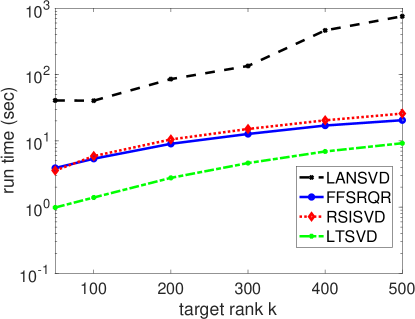
(a) Type 1: Random square matrix

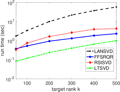
(b) Type 1: Random short-fat matrix

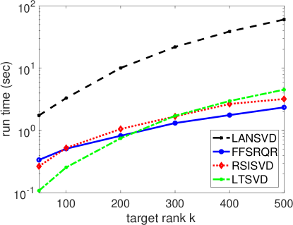
(c) Type 1: Random tall-skinny matrix

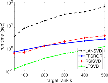
(d) Type 2: GEMAT11

Figure 1: Run time comparison for approximate SVD algorithms.

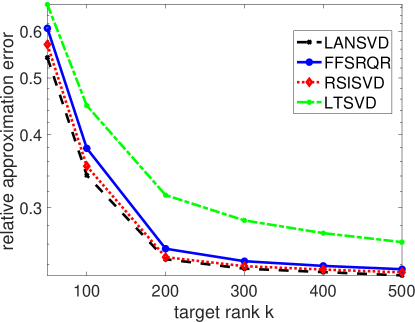
(a) Type 1: Random square matrix

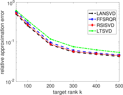
(b) Type 1: Random short-fat matrix

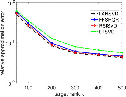
(c) Type 1: Random tall-skinny matrix

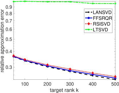
(d) Type 2: GEMAT11

Figure 2: Relative approximation error comparison for approximate SVD algorithms.

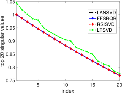
(a) Type 1: Random square matrix

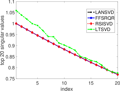
(b) Type 1: Random short-fat matrix

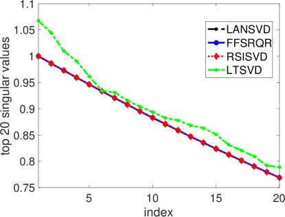
(c) Type 1: Random tall-skinny matrix

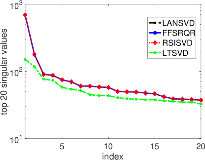
(d) Type 2: GEMAT11

Figure 3: Top 20 singular values comparison for approximate SVD algorithms.

4.2 Tensor Approximation

This section illustrates the effectiveness and efficiency of FFSRQR for computing approximate tensor. Sequentially truncated higher-order SVD (ST-HOSVD) [3, 69] is one of the most efficient algorithms to compute Tucker decomposition of tensors, and the most costing part of this algorithm is to compute SVD or approximate SVD of the tensor unfoldings. Truncated SVD and randomized SVD with subspace iteration (RSISVD) are used in routines MLSVD and MLSVD_RSI respectively in Matlab tensorlab toolbox [71]. Based on this Matlab toolbox, we implement ST-HOSVD using FFSRQR or LTSVD to do the SVD approximation. We name these two new routines by MLSVD_FFSRQR and MLSVD_LTSVD respectively. We compare these four routines in this numerical experiment. We also have Python codes for this tensor approximation numerical experiment. We don’t list the results of python here but they are similar to those of Matlab.

4.2.1 A Sparse Tensor Example

We test on a sparse tensor $\mathcal{X}\in\mathbb{R}^{n\times n\times n}$ of the following format [62, 57],

$$\mathcal{X}=\sum_{j=1}^{10}\frac{1000}{j}x_{j}\circ y_{j}\circ z_{j}+\sum_{j=11}^{n}\frac{1}{j}x_{j}\circ y_{j}\circ z_{j},$$

where $x_{j},y_{j},z_{j}\in\mathbb{R}^{n}$ are sparse vectors with nonnegative entries. The symbol “$\circ$” represents the vector outer product. We compute a rank-$\left(k,k,k\right)$ Tucker decomposition $[\mathcal{G};U_{1},U_{2},U_{3}]$ using MLSVD, MLSVD_FFSRQR, MLSVD_RSI, and MLSVD_LTSVD respectively. The relative approximation error is measured by ${\|\mathcal{X}-\mathcal{X}_{k}\|_{F}}/{\|\mathcal{X}\|_{F}}$ where $\mathcal{X}_{k}=\mathcal{G}\times_{1}U_{1}\times_{2}U_{2}\times_{3}U_{3}$.

Figure 4 compares efficiency and accuracy of different methods on a $400\times 400\times 400$ sparse tensor approximation problem. MLSVD_LTSVD is the fastest but the least accurate one. The other three methods have similar accuracy while MLSVD_FFSRQR is faster when target rank $k$ is larger.

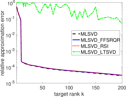
(a)

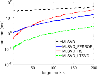
(b)

Figure 4: Run time and relative approximation error comparison on a sparse tensor.

4.2.2 Handwritten Digits Classification

MNIST is a handwritten digits image data set created by Yann LeCun [42]. Every digit is represented by a $28\times 28$ pixel image. Handwritten digits classification is to train a classification model to classify new unlabeled images. A HOSVD algorithm is proposed by Savas and Eld$\acute{e}$n [58] to classify handwritten digits. To reduce the training time, a more efficient ST-HOSVD algorithm is introduced in [69].

We do handwritten digits classification using MNIST which consists of $60,000$ training images and $10,000$ test images. The number of training images in each class is restricted to $5421$ so that the training set are equally distributed over all classes. The training set is represented by a tensor $\mathcal{X}$ of size $786\times 5421\times 10$. The classification relies on Algorithm $2$ in [58]. We use various algorithms to obtain an approximation $\mathcal{X}\approx\mathcal{G}\times_{1}U_{1}\times_{2}U_{2}\times_{3}U_{3}$ where the core tensor $\mathcal{G}$ has size $65\times 142\times 10$.

The results are summarized in Table 3. In terms of run time, our method MLSVD_FFSRQR is comparable to MLSVD_RSI while MLSVD is the most expensive one and MLSVD_LTSVD is the fastest one. In terms of classification quality, MLSVD, MLSVD_FFSRQR, and MLSVD_RSI are comparable while MLSVD_LTSVD is the least accurate one.

	MLSVD	MLSVD_FFSRQR	MLSVD_RSI	MLSVD_LTSVD
Training Time [sec]	$27.2121$	$1.5455$	$1.9343$	$0.4266$
Relative Model Error	$0.4099$	$0.4273$	$0.4247$	$0.5162$
Classification Accuracy	95.19%	94.98%	95.05%	92.59%

Table 3: Comparison on handwritten digits classification.

4.3 Solving Nuclear Norm Minimization Problem

To show the effectiveness of FFSRQR algorithm in nuclear norm minimization problems, we investigate two scenarios: robust PCA (5) and matrix completion (6). The test matrix used in robust PCA is introduced in [44] and the test matrices used in matrix completion are two real data sets. We use IALM method [44] to solve both problems and IALM’s code can be downloaded from IALM.

4.3.1 Robust PCA

To solve the robust PCA problem, we replace the approximate SVD part in IALM method [44] by various methods. We denote the actual solution to the robust PCA problem by a matrix pair $\left(X^{*},E^{*}\right)\in\mathbb{R}^{m\times n}\times\mathbb{R}^{m\times n}$. Matrix $X^{*}=X_{L}X_{R}^{T}$ where $X_{L}\in\mathbb{R}^{m\times k},~{}X_{R}\in\mathbb{R}^{n\times k}$ are random matrices where the entries are independently sampled from normal distribution. Sparse matrix $E^{*}$ is a random matrix where its non-zero entries are independently sampled from a uniform distribution over the interval $[-500,500]$. The input to the IALM algorithm has the form $M=X^{*}+E^{*}$ and the output is denoted by $\left(\widehat{X},\widehat{E}\right)$. In this numerical experiment, we use the same parameter settings as the IALM code for robust PCA: rank $k$ is $0.1m$ and number of non-zero entries in $E$ is $0.05m^{2}$. We choose the trade-off parameter $\lambda=1/\sqrt{\max\left(m,n\right)}$ as suggested by Cand$\grave{e}$s et al. [8]. The solution quality is measured by the normalized root mean square error ${\|\widehat{X}-X^{*}\|_{F}}/{\|X^{*}\|_{F}}$.

Table LABEL:Tab:_results_of_IALM_on_RPCA includes relative error, run time, the number of non-zero entries in $\widehat{E}$ ($\|\widehat{E}\|_{0}$), iteration count, and the number of non-zero singular values (#sv) in $\widehat{X}$ of IALM algorithm using different approximate SVD methods. We observe that IALM_FFSRQR is faster than all the other three methods, while its error is comparable to IALM_LANSVD and IALM_RSISVD. IALM_LTSVD is relatively slow and not effective.

Size	Method	Error	Time (sec)	$\|\widehat{E}\|_{0}$	Iter	#sv
$1000\times 1000$	IALM_LANSVD	$3.33e-07$	$5.79e+00$	$50000$	$22$	$100$
	IALM_FFSRQR	$2.79e-07$	$1.02e+00$	$50000$	$25$	$100$
	IALM_RSISVD	$3.36e-07$	$1.09e+00$	$49999$	$22$	$100$
	IALM_LTSVD	$9.92e-02$	$3.11e+00$	$999715$	$100$	$100$
$2000\times 2000$	IALM_LANSVD	$2.61e-07$	$5.91e+01$	$199999$	$22$	$200$
	IALM_FFSRQR	$1.82e-07$	$6.93e+00$	$199998$	$25$	$200$
	IALM_RSISVD	$2.63e-07$	$7.38e+00$	$199996$	$22$	$200$
	IALM_LTSVD	$8.42e-02$	$2.20e+01$	$3998937$	$100$	$200$
$4000\times 4000$	IALM_LANSVD	$1.38e-07$	$4.65e+02$	$799991$	$23$	$400$
	IALM_FFSRQR	$1.39e-07$	$4.43e+01$	$800006$	$26$	$400$
	IALM_RSISVD	$1.51e-07$	$5.04e+01$	$799990$	$23$	$400$
	IALM_LTSVD	$8.94e-02$	$1.54e+02$	$15996623$	$100$	$400$
$6000\times 6000$	IALM_LANSVD	$1.30e-07$	$1.66e+03$	$1799982$	$23$	$600$
	IALM_FFSRQR	$1.02e-07$	$1.42e+02$	$1799993$	$26$	$600$
	IALM_RSISVD	$1.44e-07$	$1.62e+02$	$1799985$	$23$	$600$
	IALM_LTSVD	$8.58e-02$	$5.55e+02$	$35992605$	$100$	$600$

Table 4: Comparison on robust PCA.

4.3.2 Matrix Completion

We solve matrix completion problems on two real data sets used in [65]: the Jester joke data set [24] and the MovieLens data set [32]. The Jester joke data set consists of $4.1$ million ratings for $100$ jokes from $73,421$ users and can be downloaded from the website Jester. We test on the following data matrices:

• jester-$1$: Data from $24,983$ users who have rated $36$ or more jokes;

• jester-$2$: Data from $23,500$ users who have rated $36$ or more jokes;

• jester-$3$: Data from $24,938$ users who have rated between $15$ and $35$ jokes;

• jester-all: The combination of jester-$1$, jester-$2$, and jester-$3$.

The MovieLens data set can be downloaded from MovieLens. We test on the following data matrices:

• movie-$100$K: $100,000$ ratings of $943$ users for $1682$ movies;

• movie-$1$M: $1$ million ratings of $6040$ users for $3900$ movies;

• movie-latest-small: $100,000$ ratings of $700$ users for $9000$ movies.

For each data set, we let $M$ be the original data matrix where $M_{ij}$ stands for the rating of joke (movie) $j$ by user $i$ and $\Gamma$ be the set of indices where $M_{ij}$ is known. The matrix completion algorithm quality is measured by the Normalized Mean Absolute Error (NMAE) which is defined by

$$\mbox{NMAE}\stackrel{{\scriptstyle def}}{{=}}\frac{\frac{1}{\left|\Gamma\right|}\sum_{\left(i,j\right)\in\Gamma}|M_{ij}-X_{ij}|}{r_{\max}-r_{\min}},$$

where $X_{ij}$ is the prediction of the rating of joke (movie) $j$ given by user $i$, and $r_{\min},r_{\max}$ are lower and upper bounds of the ratings respectively. For the Jester joke data sets we set $r_{\min}=-10$ and $r_{\max}=10$. For the MovieLens data sets we set $r_{\min}=1$ and $r_{\max}=5$.

Since $\left|\Gamma\right|$ is large, we randomly select a subset $\Omega$ from $\Gamma$ and then use Algorithm 8 to solve the problem (6). We randomly select $10$ ratings for each user in the Jester joke data sets, while we randomly choose about $50\%$ of the ratings for each user in the MovieLens data sets. Table 5 includes parameter settings in the algorithms. The maximum iteration number is $100$ in IALM, and all other parameters are the same as those used in [44].

The numerical results are included in Table 6. We observe that IALM_FFSRQR achieves almost the same recoverability as other methods except for IALM_LTSVD, and is slightly faster than IALM_RSISVD for these two data sets.

Data set	$m$	$n$	$|\Gamma|$	$|\Omega|$
jester-1	$24983$	$100$	$1.81e+06$	$249830$
jester-2	$23500$	$100$	$1.71e+06$	$235000$
jester-3	$24938$	$100$	$6.17e+05$	$249384$
jester-all	$73421$	$100$	$4.14e+06$	$734210$
moive-100K	$943$	$1682$	$1.00e+05$	$49918$
moive-1M	$6040$	$3706$	$1.00e+06$	$498742$
moive-latest-small	$671$	$9066$	$1.00e+05$	$52551$

Table 5: Parameters used in the IALM method on matrix completion.

Data set	Method	Iter	Time	NMAE	#sv	$\sigma_{\max}$	$\sigma_{min}$
jester-1	IALM-LANSVD	$12$	$7.06e+00$	$1.84e-01$	$100$	$2.14e+03$	$1.00e+00$
	IALM-FFSRQR	$12$	$3.44e+00$	$1.69e-01$	$100$	$2.28e+03$	$1.00e+00$
	IALM-RSISVD	$12$	$3.75e+00$	$1.89e-01$	$100$	$2.12e+03$	$1.00e+00$
	IALM-LTSVD	$100$	$2.11e+01$	$1.74e-01$	$62$	$3.00e+03$	$1.00e+00$
jester-2	IALM-LANSVD	$12$	$6.80e+00$	$1.85e-01$	$100$	$2.13e+03$	$1.00e+00$
	IALM-FFSRQR	$12$	$2.79e+00$	$1.70e-01$	$100$	$2.29e+03$	$1.00e+00$
	IALM-RSISVD	$12$	$3.59e+00$	$1.91e-01$	$100$	$2.12e+03$	$1.00e+00$
	IALM-LTSVD	$100$	$2.03e+01$	$1.75e-01$	$58$	$2.96e+03$	$1.00e+00$
jester-3	IALM-LANSVD	$12$	$7.05e+00$	$1.26e-01$	$99$	$1.79e+03$	$1.00e+00$
	IALM-FFSRQR	$12$	$3.03e+00$	$1.22e-01$	$100$	$1.71e+03$	$1.00e+00$
	IALM-RSISVD	$12$	$3.85e+00$	$1.31e-01$	$100$	$1.78e+03$	$1.00e+00$
	IALM-LTSVD	$100$	$2.12e+01$	$1.33e-01$	$55$	$2.50e+03$	$1.00e+00$
jester-all	IALM-LANSVD	$12$	$2.39e+01$	$1.72e-01$	$100$	$3.56e+03$	$1.00e+00$
	IALM-FFSRQR	$12$	$1.12e+01$	$1.62e-01$	$100$	$3.63e+03$	$1.00e+00$
	IALM-RSISVD	$12$	$1.34e+01$	$1.82e-01$	$100$	$3.47e+03$	$1.00e+00$
	IALM-LTSVD	$100$	$6.99e+01$	$1.68e-01$	$52$	$4.92e+03$	$1.00e+00$
moive-100K	IALM-LANSVD	$29$	$2.86e+01$	$1.83e-01$	$285$	$1.21e+03$	$1.00e+00$
	IALM-FFSRQR	$30$	$4.55e+00$	$1.67e-01$	$295$	$1.53e+03$	$1.00e+00$
	IALM-RSISVD	$29$	$4.82e+00$	$1.82e-01$	$285$	$1.29e+03$	$1.00e+00$
	IALM-LTSVD	$48$	$1.42e+01$	$1.47e-01$	$475$	$1.91e+03$	$1.00e+00$
moive-1M	IALM-LANSVD	$50$	$7.40e+02$	$1.58e-01$	$495$	$4.99e+03$	$1.00e+00$
	IALM-FFSRQR	$53$	$2.07e+02$	$1.37e-01$	$525$	$6.63e+03$	$1.00e+00$
	IALM-RSISVD	$50$	$2.23e+02$	$1.57e-01$	$495$	$5.35e+03$	$1.00e+00$
	IALM-LTSVD	$100$	$8.50e+02$	$1.17e-01$	$995$	$8.97e+03$	$1.00e+00$
moive-latest -small	IALM-LANSVD	$31$	$1.66e+02$	$1.85e-01$	$305$	$1.13e+03$	$1.00e+00$
	IALM-FFSRQR	$31$	$1.96e+01$	$2.00e-01$	$305$	$1.42e+03$	$1.00e+00$
	IALM-RSISVD	$31$	$2.85e+01$	$1.91e-01$	$305$	$1.20e+03$	$1.00e+00$
	IALM-LTSVD	$63$	$4.02e+01$	$2.08e-01$	$298$	$1.79e+03$	$1.00e+00$

Table 6: Comparison on matrix completion.

5 Conclusions

We presented the Flip-Flop SRQR factorization, a variant of QLP factorization, to compute low-rank matrix approximations. The Flip-Flop SRQR algorithm uses SRQR factorization to initialize the truncated version of column pivoted QR factorization and then form an LQ factorization. For the numerical results presented, the errors in the proposed algorithm were comparable to those obtained from the other state-of-the-art algorithms. This new algorithm is cheaper to compute and produces quality low-rank matrix approximations. Furthermore, we prove singular value lower bounds and residual error upper bounds for the Flip-Flop SRQR factorization. In situations where singular values of the input matrix decay relatively quickly, the low-rank approximation computed by SRQR is guaranteed to be as accurate as truncated SVD. We also perform complexity analysis to show that Flip-Flop SRQR is faster than approximate SVD with randomized subspace iteration. Future work includes reducing the overhead cost in Flip-Flop SRQR and implementing Flip-Flop SRQR algorithm on distributed memory machines for popular applications such as distributed PCA.

6 Appendix

6.1 Approximate SVD with Randomized Subspace Iteration

Randomized subspace iteration was proposed in [30, Algorithm 4.4] to compute an orthonormal matrix whose range approximates the range of $A$. An approximate SVD can be computed using the aforementioned orthonormal matrix [30, Algorithm 5.1]. Randomized subspace iteration is used in routine MLSVD_RSI in Matlab toolbox tensorlab [71], and MLSVD_RSI is by far the most efficient function to compute ST-HOSVD we can find in Matlab. We summarize approximate SVD with randomized subspace iteration pseudocode in Algorithm 10.

Algorithm 10 Approximate SVD with Randomized Subspace Iteration

Inputs:

Matrix $A\in\mathbb{R}^{m\times n}$. Target rank $k$. Oversampling size $p\geq 0$. Number of iterations $q\geq 1$.

Outputs:

$U\in\mathbb{R}^{m\times k}$ contains the approximate top $k$ left singular vectors of $A$.

$\Sigma\in\mathbb{R}^{k\times k}$ contains the approximate top $k$ singular values of $A$.

$V\in\mathbb{R}^{n\times k}$ contains the approximate top $k$ right singular vectors of $A$.

Algorithm:

Generate i.i.d Gaussian matrix $\Omega\in\mathcal{N}\left(0,1\right)^{n\times\left(k+p\right)}$.

Compute $B=A\Omega$.

$[Q,\sim]=qr\left(B,0\right)$

for $i=1:q$ do

   $B=A^{T}*Q$

   $[Q,\sim]=qr\left(B,0\right)$

   $B=A*Q$

   $[Q,\sim]=qr\left(B,0\right)$

end for

$B=Q^{T}*A$

$[U,\Sigma,V]=svd\left(B\right)$

$U=Q*U$

$U=U\left(:,1:k\right)$

$\Sigma=\Sigma\left(1:k,1:k\right)$

$V=V\left(:,1:k\right)$

Now we perform a complexity analysis on approximate SVD with randomized subspace iteration. We first note that

1. The cost of generating a random matrix is negligible.

2. The cost of computing $B=A\Omega$ is $2mn\left(k+p\right)$.

3. In each QR step $[Q,\sim]=qr\left(B,0\right)$, the cost of computing the QR factorization of $B$ is $2m\left(k+p\right)^{2}-\frac{2}{3}\left(k+p\right)^{3}$ (c.f. [66]), and the cost of forming the first $\left(k+p\right)$ columns in the full $Q$ matrix is $m\left(k+p\right)^{2}+\frac{1}{3}\left(k+p\right)^{3}$.

Now we count the flops for each $i$ in the ${\bf for}$ loop:

1. The cost of computing $B=A^{T}*Q$ is $2mn\left(k+p\right)$;

2. The cost of computing $[Q,\sim]=qr\left(B,0\right)$ is $2n\left(k+p\right)^{2}-\frac{2}{3}\left(k+p\right)^{3}$, and the cost of forming the first $\left(k+p\right)$ columns in the full $Q$ matrix is $n\left(k+p\right)^{2}+\frac{1}{3}\left(k+p\right)^{3}$;

3. The cost of computing $B=A*Q$ is $2mn\left(k+p\right)$;

4. The cost of computing $[Q,\sim]=qr\left(B,0\right)$ is $2m\left(k+p\right)^{2}-\frac{2}{3}\left(k+p\right)^{3}$, and the cost of forming the first $\left(k+p\right)$ columns in the full $Q$ matrix is $m\left(k+p\right)^{2}+\frac{1}{3}\left(k+p\right)^{3}$.

Putting together, the cost of running the ${\bf for}$ loop $q$ times is

$$q\left(4mn\left(k+p\right)+3\left(m+n\right)\left(k+p\right)^{2}-\frac{2}{3}\left(k+p\right)^{3}\right).$$

Additionally, the cost of computing $B=Q^{T}*A$ is $2mn\left(k+p\right)$; the cost of doing SVD of $B$ is $O(n\left(k+p\right)^{2})$; and the cost of computing $U=Q*U$ is $2m\left(k+p\right)^{2}$.

Now assume $k+p\ll\min\left(m,n\right)$ and omit the lower-order terms, then we arrive at $\left(4q+4\right)mn\left(k+p\right)$ as the complexity of approximate SVD with randomized subspace iteration. In practice, $q$ is usually chosen to be an integer between $0$ and $2$.

References

- [1] O. Alter, P. O. Brown, and D. Botstein, Singular value decomposition for genome-wide expression data processing and modeling, Proceedings of the National Academy of Sciences, 97 (2000), pp. 10101–10106.
- [2] E. Anderson, Z. Bai, C. Bischof, L. S. Blackford, J. Demmel, J. Dongarra, J. Du Croz, A. Greenbaum, S. Hammarling, and A. McKenney, LAPACK Users’ Guide, SIAM, Philadelphia, 1999.
- [3] C. A. Andersson and R. Bro, Improving the speed of multi-way algorithms: Part I. Tucker3, Chemometrics and Intelligent Laboratory Systems, 42 (1998), pp. 93–103.
- [4] M. W. Berry, S. T. Dumais, and G. W. O’Brien, Using linear algebra for intelligent information retrieval, SIAM Review, 37 (1995), pp. 573–595.
- [5] C. Bischof and C. Van Loan, The WY representation for products of Householder matrices, SIAM Journal on Scientific and Statistical Computing, 8 (1987), pp. s2–s13.
- [6] P. Businger and G. H. Golub, Linear least squares solutions by Householder transformations, Numerische Mathematik, 7 (1965), pp. 269–276.
- [7] J.-F. Cai, E. J. Candès, and Z. Shen, A singular value thresholding algorithm for matrix completion, SIAM Journal on Optimization, 20 (2010), pp. 1956–1982.
- [8] E. J. Candès, X. Li, Y. Ma, and J. Wright, Robust principal component analysis?, Journal of the ACM (JACM), 58 (2011), pp. 11:1–11:37.
- [9] E. J. Candès and B. Recht, Exact matrix completion via convex optimization, Foundations of Computational Mathematics, 9 (2009), pp. 717–772.
- [10] J. D. Carroll and J.-J. Chang, Analysis of individual differences in multidimensional scaling via an N-way generalization of ”Eckart-Young” decomposition, Psychometrika, 35 (1970), pp. 283–319.
- [11] T. A. Davis and Y. Hu, The university of florida sparse matrix collection, ACM Transactions on Mathematical Software (TOMS), 38 (2011), pp. 1:1–1:25.
- [12] L. De Lathauwer and B. De Moor, From matrix to tensor: Multilinear algebra and signal processing, in Mathematics in Signal Processing IV, J. McWhirter and E. I. Proudler, eds., Clarendon Press, Oxford, UK, 1998, pp. 1–15.
- [13] L. De Lathauwer, B. De Moor, and J. Vandewalle, A multilinear singular value decomposition, SIAM journal on Matrix Analysis and Applications, 21 (2000), pp. 1253–1278.
- [14] L. De Lathauwer, B. De Moor, and J. Vandewalle, On the best rank-1 and rank-() approximation of higher-order tensors, SIAM journal on Matrix Analysis and Applications, 21 (2000), pp. 1324–1342.
- [15] L. De Lathauwer and J. Vandewalle, Dimensionality reduction in higher-order signal processing and rank-() reduction in multilinear algebra, Linear Algebra and its Applications, 391 (2004), pp. 31–55.
- [16] V. De Silva and L.-H. Lim, Tensor rank and the ill-posedness of the best low-rank approximation problem, SIAM Journal on Matrix Analysis and Applications, 30 (2008), pp. 1084–1127.
- [17] P. Drineas, R. Kannan, and M. W. Mahoney, Fast Monte Carlo algorithms for matrices II: Computing a low-rank approximation to a matrix, SIAM Journal on computing, 36 (2006), pp. 158–183.
- [18] J. A. Duersch and M. Gu, Randomized QR with column pivoting, SIAM Journal on Scientific Computing, 39 (2017), pp. C263–C291.
- [19] C. Eckart and G. Young, The approximation of one matrix by another of lower rank, Psychometrika, 1 (1936), pp. 211–218.
- [20] L. Eldén, Matrix Methods in Data Mining and Pattern Recognition, SIAM, Philadelphia, 2007.
- [21] M. Fazel, Matrix Rank Minimization with Applications, PhD thesis, Stanford University, Stanford, CA, 2002.
- [22] M. Fazel, H. Hindi, and S. P. Boyd, Log-det heuristic for matrix rank minimization with applications to Hankel and Euclidean distance matrices, in Proceedings of the 2003 American Control Conference, vol. 3, 2003, pp. 2156–2162.
- [23] G. W. Furnas, S. Deerwester, S. T. Dumais, T. K. Landauer, R. A. Harshman, L. A. Streeter, and K. E. Lochbaum, Information retrieval using a singular value decomposition model of latent semantic structure, in Proceedings of the 11th Annual International ACM SIGIR Conference on Research and Development in Information Retrieval, ACM, 1988, pp. 465–480.
- [24] K. Goldberg, T. Roeder, D. Gupta, and C. Perkins, Eigentaste: A constant time collaborative filtering algorithm, Information Retrieval, 4 (2001), pp. 133–151.
- [25] G. Golub, Numerical methods for solving linear least squares problems, Numerische Mathematik, 7 (1965), pp. 206–216.
- [26] G. H. Golub and C. F. Van Loan, Matrix Computations, Johns Hopkins University Press, 3rd ed., 2012.
- [27] M. Gu, Subspace iteration randomization and singular value problems, SIAM Journal on Scientific Computing, 37 (2015), pp. A1139–A1173.
- [28] M. Gu and S. C. Eisenstat, Efficient algorithms for computing a strong rank-revealing QR factorization, SIAM Journal on Scientific Computing, 17 (1996), pp. 848–869.
- [29] E. T. Hale, W. Yin, and Y. Zhang, Fixed-point continuation for -minimization: Methodology and convergence, SIAM Journal on Optimization, 19 (2008), pp. 1107–1130.
- [30] N. Halko, P.-G. Martinsson, and J. A. Tropp, Finding structure with randomness: Probabilistic algorithms for constructing approximate matrix decompositions, SIAM Review, 53 (2011), pp. 217–288.
- [31] R. A. Harshman, Foundations of the PARAFAC procedure: Models and conditions for an ”explanatory” multimodal factor analysis, UCLA Working Papers in Phonetics, 16 (1970), pp. 1–84, http://www.psychology.uwo.ca/faculty/harshman/wpppfac0.pdf.
- [32] J. L. Herlocker, J. A. Konstan, A. Borchers, and J. Riedl, An algorithmic framework for performing collaborative filtering, in Proceedings of the 22nd Annual International ACM SIGIR Conference on Research and Development in Information Retrieval, ACM, 1999, pp. 230–237.
- [33] R. A. Horn and C. R. Johnson, Topics in Matrix Analysis, Cambridge University Press, 1991.
- [34] D. Huckaby and T. F. Chan, On the convergence of Stewart’s QLP algorithm for approximating the SVD, Numerical Algorithms, 32 (2003), pp. 287–316.
- [35] D. Huckaby and T. F. Chan, Stewart’s pivoted QLP decomposition for low-rank matrices, Numerical Linear Algebra with Applications, 12 (2005), pp. 153–159.
- [36] I. T. Jolliffe, Principal Component Analysis, Springer-Verlag, New York, 1986.
- [37] J. M. Kleinberg, Authoritative sources in a hyperlinked environment, Journal of the ACM (JACM), 46 (1999), pp. 604–632.
- [38] T. G. Kolda, Orthogonal tensor decompositions, SIAM Journal on Matrix Analysis and Applications, 23 (2001), pp. 243–255.
- [39] T. G. Kolda and B. W. Bader, Tensor decompositions and applications, SIAM Review, 51 (2009), pp. 455–500.
- [40] R. M. Larsen, Lanczos bidiagonalization with partial reorthogonalization, DAIMI Report Series, 27 (1998).
- [41] R. M. Larsen, PROPACK - software for large and sparse SVD calculations, 1998, http://sun.stanford.edu/~rmunk/PROPACK/.
- [42] Y. LeCun, L. Bottou, Y. Bengio, and P. Haffner, Gradient-based learning applied to document recognition, Proceedings of the IEEE, 86 (1998), pp. 2278–2324.
- [43] R. B. Lehoucq, D. C. Sorensen, and C. Yang, ARPACK Users’ Guide: Solution of Large-Scale Eigenvalue Problems with Implicitly Restarted Arnoldi Methods, SIAM, Philadelphia, 1998.
- [44] Z. Lin, M. Chen, and Y. Ma, The augmented Lagrange multiplier method for exact recovery of corrupted low-rank matrices, Sep. 2010, https://arxiv.org/abs/1009.5055.
- [45] N. Linial, E. London, and Y. Rabinovich, The geometry of graphs and some of its algorithmic applications, Combinatorica, 15 (1995), pp. 215–245.
- [46] Z. Liu, A. Hansson, and L. Vandenberghe, Nuclear norm system identification with missing inputs and outputs, Systems & Control Letters, 62 (2013), pp. 605–612.
- [47] Z. Liu and L. Vandenberghe, Interior-point method for nuclear norm approximation with application to system identification, SIAM Journal on Matrix Analysis and Applications, 31 (2009), pp. 1235–1256.
- [48] S. Ma, D. Goldfarb, and L. Chen, Fixed point and Bregman iterative methods for matrix rank minimization, Mathematical Programming, 128 (2011), pp. 321–353.
- [49] M. Mesbahi and G. P. Papavassilopoulos, On the rank minimization problem over a positive semidefinite linear matrix inequality, IEEE Transactions on Automatic Control, 42 (1997), pp. 239–243.
- [50] N. Muller, L. Magaia, and B. M. Herbst, Singular value decomposition, eigenfaces, and 3D reconstructions, SIAM Review, 46 (2004), pp. 518–545.
- [51] M. Narwaria and W. Lin, SVD-based quality metric for image and video using machine learning, IEEE Transactions on Systems, Man, and Cybernetics, Part B (Cybernetics), 42 (2012), pp. 347–364.
- [52] T.-H. Oh, Y. Matsushita, Y.-W. Tai, and I. So Kweon, Fast randomized singular value thresholding for nuclear norm minimization, in Proceedings of the IEEE Conference on Computer Vision and Pattern Recognition, 2015, pp. 4484–4493.
- [53] G. Quintana-Ortí, X. Sun, and C. H. Bischof, A BLAS-3 version of the QR factorization with column pivoting, SIAM Journal on Scientific Computing, 19 (1998), pp. 1486–1494.
- [54] B. Recht, M. Fazel, and P. A. Parrilo, Guaranteed minimum-rank solutions of linear matrix equations via nuclear norm minimization, SIAM Review, 52 (2010), pp. 471–501.
- [55] J. D. Rennie and N. Srebro, Fast maximum margin matrix factorization for collaborative prediction, in Proceedings of the 22nd International Conference on Machine Learning, ACM, 2005, pp. 713–719.
- [56] V. Rokhlin, A. Szlam, and M. Tygert, A randomized algorithm for principal component analysis, SIAM Journal on Matrix Analysis and Applications, 31 (2009), pp. 1100–1124.
- [57] A. K. Saibaba, HOID: Higher Order Interpolatory Decomposition for tensors based on Tucker representation, SIAM Journal on Matrix Analysis and Applications, 37 (2016), pp. 1223–1249.
- [58] B. Savas and L. Eldén, Handwritten digit classification using higher order singular value decomposition, Pattern recognition, 40 (2007), pp. 993–1003.
- [59] R. Schreiber and C. Van Loan, A storage-efficient WY representation for products of Householder transformations, SIAM Journal on Scientific and Statistical Computing, 10 (1989), pp. 53–57.
- [60] A. Shashua and T. Hazan, Non-negative tensor factorization with applications to statistics and computer vision, in Proceedings of the 22nd International Conference on Machine Learning, ACM, 2005, pp. 792–799.
- [61] N. D. Sidiropoulos, R. Bro, and G. B. Giannakis, Parallel factor analysis in sensor array processing, IEEE transactions on Signal Processing, 48 (2000), pp. 2377–2388.
- [62] D. C. Sorensen and M. Embree, A DEIM induced CUR factorization, SIAM Journal on Scientific Computing, 38 (2016), pp. A1454–A1482.
- [63] N. Srebro, J. Rennie, and T. S. Jaakkola, Maximum-margin matrix factorization, in Advances in neural information processing systems, 2005, pp. 1329–1336.
- [64] G. Stewart, The QLP approximation to the singular value decomposition, SIAM Journal on Scientific Computing, 20 (1999), pp. 1336–1348.
- [65] K.-C. Toh and S. Yun, An accelerated proximal gradient algorithm for nuclear norm regularized linear least squares problems, Pacific Journal of Optimization, 6 (2010), pp. 615–640.
- [66] L. N. Trefethen and D. Bau III, Numerical Linear Algebra, vol. 50, SIAM, Philadelphia, 1997.
- [67] L. R. Tucker, Some mathematical notes on three-mode factor analysis, Psychometrika, 31 (1966), pp. 279–311.
- [68] M. Turk and A. Pentland, Eigenfaces for recognition, Journal of Cognitive Neuroscience, 3 (1991), pp. 71–86.
- [69] N. Vannieuwenhoven, R. Vandebril, and K. Meerbergen, A new truncation strategy for the higher-order singular value decomposition, SIAM Journal on Scientific Computing, 34 (2012), pp. A1027–A1052.
- [70] M. A. O. Vasilescu and D. Terzopoulos, Multilinear analysis of image ensembles: Tensorfaces, in European Conference on Computer Vision, Springer, 2002, pp. 447–460.
- [71] N. Vervliet, O. Debals, L. Sorber, M. V. Barel, and L. De Lathauwer, Tensorlab 3.0, 2016, http://www.tensorlab.net.
- [72] H. Wang and N. Ahuja, Facial expression decomposition, in Proceedings of the 9th IEEE International Conference on Computer Vision (ICCV), 2003, pp. 958–965.
- [73] J. Xiao and M. Gu, Spectrum-revealing Cholesky factorization for kernel methods, in Proceedings of the 16th IEEE International Conference on Data Mining (ICDM), 2016, pp. 1293–1298.
- [74] J. Xiao, M. Gu, and J. Langou, Fast parallel randomized QR with column pivoting algorithms for reliable low-rank matrix approximations, in Proceedings of the 24th IEEE International Conference on High Performance Computing (HiPC), 2017, pp. 233–242.
- [75] T. Zhang and G. H. Golub, Rank-one approximation to high order tensors, SIAM Journal on Matrix Analysis and Applications, 23 (2001), pp. 534–550.