Supersymmetry versus Compositeness: 2HDMs tell the story

Abstract

Supersymmetry and Compositeness are two prevalent paradigms providing both a solution to the hierarchy problem and a motivation for a light Higgs boson state. As the latter has now been found, its dynamics can hold the key to disentangle the two theories. An open door towards the solution is found in the context of 2-Higgs Doublet Models (2HDMs), which are necessary to Supersymmetry and natural within Compositeness in order to enable Electro-Weak Symmetry Breaking. We show how 2HDM spectra of masses and couplings accessible at the Large Hadron Collider may allow one to separate the two scenarios.

Introduction – What has been the discovery of the cornerstone of the Standard Model (SM), the Higgs boson, should now turn out to be the stepping stone into a new physics world. The latter is currently unknown to us. We know though what its dynamics should prevent, i.e., the hierarchy problem. There are two possible pathways to follow in the quest for Beyond the SM (BSM) physics which would at once reconcile the above experimental and theoretical instances. These are Supersymmetry and Compositeness. The former predicts a light Higgs boson as it relates its trilinear self-coupling (hence its mass) to the smallness of the gauge couplings and avoids the hierarchy problem thanks to the presence of supersymmetric counterparts, of different statistics with respect to the SM objects (a boson for a fermion, and vice versa), which then cancel divergent contributions to the Higgs mass. In fact, both conditions are achieved most effectively when the top quark partner in Supersymmetry, the stop, has a mass above the TeV scale, thereby lifting the tree-level Higgs boson mass from below $M_{Z}$ to the measured value of 125 GeV or so. The latter can also naturally embed a light Higgs state, as a pseudo Nambu-Goldstone Boson (pNGB), if the top quark composite counterparts are at the TeV scale.

It is thus evident that, despite the different principles behind the two theories, the low energy phenomenology of their Higgs and top partner sectors may be rather similar. However, in this connection, we shall prove here that differences exist between these two BSM scenarios that can presently be tested at the Large Hadron Collider (LHC). This can become manifest if one realises that an enlarged Higgs sector, notably involving a 2-Higgs Doublet Model (2HDM) dynamics, is required by Supersymmetry and natural in Compositeness. By exploiting a recently completed calculation of the Higgs potential BigPaper in a Composite 2HDM (C2HDM), we will contrast the ensuing results concerning Higgs boson masses and couplings to the well known ones established in Supersymmetry Djouadi .

Explicit Model – We now give a brief setup for our C2HDM construction to describe the salient features of the numerical results shown below. Details will be illustrated in BigPaper . We consider a spontaneous global symmetry breaking $SO(6)\to SO(4)\times SO(2)$ at a (Compositeness) scale $f$ providing two pNGB doublets. The pNGB matrix $U$ is constructed from the 8 broken $SO(6)$ generators ($T^{\hat{a}}_{i}$, $i=1,2$, $\hat{a}=1,\dots,4$) out of the 15 total ones ($T^{A}$, $A=1,\dots,15$) as

$$U=e^{i\frac{\Pi}{f}},\quad\Pi\equiv\sqrt{2}\phi_{i}^{\hat{a}}T^{\hat{a}}_{i}=-i\begin{pmatrix}0_{4\times 4}&{\bf\Phi}\\ -{\bf\Phi}^{T}&0_{2\times 2}\end{pmatrix},$$ (1)

where ${\bf\Phi}\equiv(\phi_{1}^{\hat{a}},\phi_{2}^{\hat{a}})$. The two real 4–vectors $\phi_{i}^{\hat{a}}$ can be rearranged into two complex doublets $\Phi_{i}$ ($i=1,2$), as

$$\Phi_{i}=\frac{1}{\sqrt{2}}\left(\begin{array}[]{cc}\phi_{i}^{\hat{2}}+i\phi_{i}^{\hat{1}}\\ \phi_{i}^{\hat{4}}-i\phi_{i}^{\hat{3}}\end{array}\right).$$ (4)

The Vacuum Expectation Values (VEVs) of the Higgs fields are taken to be $\langle\phi_{i}^{\hat{4}}\rangle=v_{i}$, so we define $v^{2}=v_{1}^{2}+v_{2}^{2}$ and $\tan\beta=v_{2}/v_{1}$ as usual in 2HDMs. Because of the non-linear nature of the pNGBs eventually emerging as Higgs boson states, $v$ does not correspond to the SM Higgs VEV $v_{\text{SM}}$ (related to the Fermi constant $G_{F}$ by $v_{\text{SM}}^{2}=(\sqrt{2}G_{F})^{-1}$), rather, it satisfies the relation

$$v_{\text{SM}}^{2}=f^{2}\sin^{2}\frac{v}{f}.$$ (5)

In order to obtain a non-zero value for the Higgs boson masses, explicit breaking terms of the $SO(6)$ symmetry must be introduced. Within the partial Compositeness paradigm partial , this can be achieved by a linear mixing between the (elementary) SM and (composite) strong sector fields, where the former and the latter are described, respectively, by $SU(2)_{L}\times U(1)_{Y}$ and $SO(6)\times U(1)_{X}$ representations. Notice that, in the strong sector, the $U(1)_{X}$ symmetry is necessary to correctly realise the $U(1)_{Y}$ hypercharge charge assignment of the SM fermions. Thus, the Lagrangian is

$${\cal L}={\cal L}_{\text{SM}}+{\cal L}_{\text{strong}}+{\cal L}_{\text{mix}},$$ (6)

where ${\cal L}_{\text{SM}}$ denotes the Lagrangian of kinetic terms for the SM gauge bosons ($W_{\mu}^{a}$ and $B_{\mu}$) and fermions (for the computation of the scalar potential it is sufficient to consider only the third generation of the left-handed quark doublets $q_{L}$ and right-handed top quark $t_{R}$), while ${\cal L}_{\text{strong}}$ and ${\cal L}_{\text{mix}}$ represent the Lagrangian of the strong sector and the mixing one, respectively.

For an explicit realisation of this setup, it is convenient to define the elementary fields as incomplete $SO(6)$ multiplets by introducing spurion fields. Namely, the elementary gauge bosons can be embedded into $SO(6)$ adjoint $(A_{\mu}^{A})$ and $U(1)_{X}$ $(X_{\mu})$ spurion fields, while the elementary fermions can be embedded into the $SO(6)$ ${\bf 6}$-plet spurions $q_{L}^{\bf{6}}$ and $t_{R}^{\bf{6}}$.

The explicit model is based on the 2-site construction defined in Ref. 4dchm . The extra degrees of freedom in the gauge sector are the spin-1 resonances of the adjoint of $SO(6)$ ($\rho^{A}$) and $U(1)_{X}$ ($\rho_{X}$). The gauge sector for ${\cal L}_{\text{strong}}$ and ${\cal L}_{\text{mix}}$ is then given by

$${\cal L}_{\text{strong}}^{\text{gauge}}+{\cal L}_{\text{mix}}^{\text{gauge}}=-\frac{1}{4g_{\rho}^{2}}\rho^{A}_{\mu\nu}\rho^{A\mu\nu}-\frac{1}{4g_{\rho_{X}}^{2}}\rho_{X\mu\nu}\rho_{X}^{\mu\nu}$$

$$~{}~{}+\frac{f_{1}^{2}}{4}\text{tr}(D_{\mu}U_{1})^{\dagger}(D_{\mu}U_{1})+\frac{f_{2}^{2}}{4}\text{tr}(D_{\mu}\Sigma_{2})^{T}(D^{\mu}\Sigma_{2}),$$ (7)

where $U_{i}=e^{i\frac{f}{f_{i}^{2}}\Pi}$, $U=U_{1}U_{2}$ and $\Sigma_{i}=U_{i}\Sigma_{0}U_{i}^{T}~{}(i=1,2)$, with $f^{-2}=f_{1}^{-2}+f_{2}^{-2}$ and $\Sigma_{0}=0_{4\times 4}\oplus i\sigma_{2}$ being an $SO(4)\times SO(2)$ invariant vacuum. Also,

$$D_{\mu}U_{1}=\partial_{\mu}U_{1}-iA_{\mu}U_{1}+iU_{1}\rho_{\mu},$$

$$D_{\mu}\Sigma_{2}=\partial_{\mu}\Sigma_{2}-i[\rho_{\mu},\Sigma_{2}],$$ (8)

where $\rho_{\mu}\equiv\rho_{\mu}^{A}T^{A}+\rho_{\mu}^{X}T^{X}$ and $A_{\mu}\equiv A_{\mu}^{A}T^{A}+X_{\mu}T^{X}$.

In the fermion sector we consider $N$ spin $1/2$ resonances $\Psi^{I}$ ($I=1,\dots,N$) which are $SO(6)$ ${\bf 6}$-plets with $X=2/3$. The corresponding Lagrangian is

$${\cal L}_{\text{strong}}^{\text{ferm}}+{\cal L}_{\text{mix}}^{\text{ferm}}=\bar{\Psi}^{I}iD/\hskip 1.70717pt\Psi^{I}-\bar{\Psi}_{L}^{I}M_{\Psi}^{IJ}\Psi_{R}^{J}-\bar{\Psi}_{L}^{I}(Y_{1}^{IJ}\Sigma_{2}$$

$$+{Y}_{2}^{IJ}\Sigma_{2}^{2})\Psi_{R}^{J}+(\Delta_{L}^{I}\bar{q}_{L}^{\bf{6}}U_{1}\Psi_{R}^{I}+\Delta_{R}^{I}\bar{t}_{R}^{\bf{6}}U_{1}\Psi_{L}^{I})+\text{h.c.},$$ (9)

where $\Delta_{L,R}$ ($M_{\Psi}$, $Y_{1}$ and ${Y}_{2}$) are dimensionful $N$–vectors ($N\times N$ matrices). Since $\Sigma_{2}^{3}=-\Sigma_{2}$, terms up to quadratic power in $\Sigma_{2}$ reproduce the most general interaction Lagrangian between the fermionic resonances and the pNGB fields. For simplicity, we assume CP-conservation in the strong sector, i.e., all parameters in Eq. (9) to be real. As a result, the Coleman-Weinberg (CW) Higgs potential is CP-conserving. The Yukawa interactions for the right-handed bottom quark can also be included by introducing further spin-1/2 resonances with $X=-1/3$. Analogously one can implement partial Compositeness for tau leptons too.

We note that the gauge interactions do not give rise to Ultra–Violet (UV) divergences in the calculation of the Higgs potential, on the contrary, the fermion Lagrangian defined above provides logarithmic UV divergences which can be removed by suitable conditions among the parameters. In the $N=2$ case, we can easily derive the conditions for cancellation of the UV divergences in the CW potential (see BigPaper ) and, among all possible solutions, the enforcement of the “left-right symmetry” defined in Ref. 4dchm provides the following simple setup, which will be adopted in our analysis:

$$\Delta_{L}^{2}=\Delta_{R}^{1}=0,\quad Y_{2}^{11}=M_{\Psi}^{11},\quad M_{\Psi}^{21}=0,$$

$$Y_{1}^{11}=Y_{1}^{22}=Y_{1}^{21}=Y_{2}^{21}=Y_{2}^{22}=0.$$ (10)

The low energy Lagrangian for the quark fields, obtained from Eq. (9) after the integration of the heavy degrees of freedom, introduces, in general, Flavour Changing Neutral Currents (FCNCs) at tree level via Higgs boson exchanges. There are basically two ways to avoid such FCNCs. The first one is to impose a $C_{2}$ symmetry Mrazek , just like in $Z_{2}$ symmetric Elementary 2HDMs (E2HDMs), which would forbid the $Y_{1}$ term. The $C_{2}$ symmetric scenario exactly reproduces a composite realisation of the inert 2HDM. In this case the couplings to the SM fields of the SM-like Higgs boson, arising from the $C_{2}$-even doublet, are the same as in the minimal composite Higgs model 4dchm , while the lightest component of the $C_{2}$-odd doublet could potentially account for a dark matter candidate. Here we will follow an alternative approach with a broken $C_{2}$ which requires an alignment between the two matrices $Y_{1}$ and $Y_{2}$. Under this assumption, the latter two, for each type of fermions in the low energy Lagrangian, become proportional to each other, like in the Aligned 2HDM (A2HDM) a2hdm .

Let us now describe the main steps of the calculation of the Higgs potential. Integrating out the heavy spin-1 ($\rho^{A}$ and $\rho_{X}$) and 1/2 ($\Psi^{I}$) states, we obtain the effective low-energy Lagrangian for the SM gauge bosons, the SM quark fields and the Higgs fields $\Phi_{i}$. In each coefficient of the Lagrangian terms, form factors appear, which are expressed as functions of the parameters of the strong sector. Their explicit forms are provided in BigPaper . The Higgs potential is then generated via the CW mechanism by the gauge boson ($W_{\mu}^{a}$ and $B_{\mu}$) and fermion ($q_{L}$ and $t_{R}$) loop contributions. As already mentioned, UV divergences do not appear by virtue of the UV-finiteness conditions given in Eq. (10). By expanding up to the fourth order in the $\Phi_{i}$ fields we get

$$iV\simeq\frac{1}{f^{4}}\int\frac{d^{4}k}{(2\pi)^{4}}\left[\frac{3}{2}V_{G}(\Phi_{1},\Phi_{2})-6V_{F}(\Phi_{1},\Phi_{2})\right],$$ (11)

where $V_{G,F}(\Phi_{1},\Phi_{2})$ are characterised by the same structure of the Higgs potential in E2HDMs written in terms of 3 dimensionful mass parameters ($m_{11}^{2}$, $m_{22}^{2}$ and $m_{12}^{2}$) and 7 dimensionless couplings $\lambda_{i}$ ($i=1,\dots,7$) (see, e.g., Ref. Branco for the definition of these coefficients). In general, $m_{12}^{2}$ and $\lambda_{5,6,7}$ can be complex, but they are found to be real as a consequence of the requirement of CP-conservation in the strong sector. These coefficients are determined in terms of the parameters of the strong sector. Therefore, the masses of the Higgs bosons and the scalar mixing angle are fully predicted by the strong dynamics.

Results – For our numerical analysis, we take $f_{1}=f_{2}$, $g_{\rho}=g_{\rho_{X}}$ and $M_{\Psi}^{11}=M_{\Psi}^{22}=M_{\Psi}$. Then, we have 8 free parameters of the strong sector, i.e.,

$$f,~{}g_{\rho},~{}Y_{1}^{12},~{}Y_{2}^{12},~{}\Delta_{L}^{1},~{}\Delta_{R}^{2},~{}M_{\Psi},~{}M_{\Psi}^{12}.$$ (12)

In order to have phenomenologically acceptable configurations, other than ensuring Electro-Weak Symmetry Breaking (EWSB), with EW parameters consistent with data, we further require: (i) the vanishing of the two tadpoles of the CP-even Higgs bosons, (ii) the predicted top mass to be $165~{}\textrm{GeV}<m_{t}<175$ GeV and (iii) the predicted Higgs boson mass to be $120~{}\textrm{GeV}<m_{h}<130$ GeV. Under these constraints, we scan the parameters shown in Eq. (12) within the ranges $0\leq X\leq 10f$ ($X=Y_{1}^{12},~{}Y_{2}^{12},~{}\Delta_{L}^{1},~{}\Delta_{R}^{2},~{}M_{\Psi},~{}M_{\Psi}^{12}$), $600$ GeV $\leq f\leq 3000$ GeV. Hereafter, $g_{\rho}$ is fixed to be 5. As outputs, we obtain the masses of the charged Higgs boson $(m_{H^{\pm}})$, the CP-odd Higgs boson ($m_{A}$), the heavier CP-even Higgs boson ($m_{H}$) and the mixing angle $\theta$ between the two CP-even Higgs boson states ($h,H$). Equipped with the mass and coupling spectrum of the C2HDM, we have also tested its parameter space against experimental Higgs boson data using HiggsBounds-5 and HiggsSignals-2 Bechtle:2013wla ; Bechtle:2013xfa .

We highlight next the main differences between our C2HDM and the Minimal Supersymmetric SM (MSSM), both of which can be regarded as the minimal realisations of EWSB based on a 2HDM structure embedded in Compositeness and Supersymmetry, respectively. (In the MSSM, the latter is a Type-II one). For the MSSM predictions, we employ FeynHiggs 2.14.1 Heinemeyer:1998yj ; Hahn:2013ria and scan the parameter space according to the recommendations provided in Bagnaschi:2015hka .

1. Prediction of $\tan\beta$ and Higgs Boson Masses – While in the MSSM the parameter $\tan\beta$ is essentially a free one, albeit potentially limited by theoretically and experimentally constraints, in the C2HDM it is predicted and correlates strongly to $f$. This is illustrated in Fig. 1. We note that all scan points are randomly generated, so that their density is a measure of probability of a region of parameter space to meet the above constraints. Clearly, it is seen that the density of the allowed points become smaller in regions with larger values of $f$ and/or $\tan\beta$. This can be understood by the fact that departure from $f\sim v_{\textrm{SM}}$ requires fine-tuning among the strong parameters, in order to satisfy the tadpole conditions and reconstruct the observed $m_{h}$ and $m_{t}$ values. In fact, this behaviour has also been known in minimal composite Higgs models, see e.g., Panico:2012uw . Therefore, in the C2HDM, small $f$ (well within the LHC energy domain) and $\tan\beta\sim{\cal O}(1)$ (indeed, solutions above $\tan\beta\sim 10$ are highly disfavoured by requiring $m_{h}\sim 125$ GeV and $m_{t}\sim 170$ GeV) are naturally predicted. Further, for any $f$ value, we notice that $\tan\beta$ values between (somewhat above) 1 and 6 are more favoured than others. Hence, in the following, we will at times single out this region of parameter space.

However, this result does not imply that the parameter space of the Higgs sector of the C2HDM is reduced with respect to that of the MSSM, where $\tan\beta$ can in general take values between 1 and, say, $\bar{m}_{t}/\bar{m}_{b}\approx 45$ (with $\bar{m}_{{b,t}}$ being the running masses of the $b,t$-quarks computed at $m_{h}$), compatible with Supersymmetry unification conditions other than compliant with theoretical and experimental constraints. In fact, it should be recalled that $\tan\beta$ is not, in general, a fundamental parameter of a 2HDM, as explained in Davidson:2005cw ; Haber:2006ue ; Haber:2010bw , since it is not basis-independent and a one-to-one comparison of models for fixed values of $\tan\beta$ is not meaningful unless the realisation of the 2HDM is the same, namely, the models share the same discrete symmetries. While the MSSM is characterised by a Type-II 2HDM structure, with $\tan\beta$ defined in the basis where the discrete symmetry of the two Higgs doublets is manifest, the C2HDM considered in this work does not possess a $C_{2}$ symmetry. Even though the strong sector uniquely identifies a special basis for the Higges and, thus, selects a special $\tan\beta$ among all possible basis-dependent definitions (see BigPaper for more details), this parameter cannot be directly compared to the MSSM one. Therefore, when comparing physical observables in the composite and supersymmetric scenarios, one should inclusively span $\tan\beta$ between 1 and 45 for the MSSM and over all predicted values (see Fig. 1) for the C2HDM.

Other than $\tan\beta$, also the Higgs masses are predicted in the C2HDM, e.g., $m_{A}$ is shown in Fig. 3. In the MSSM, in contrast, $m_{A}$ is normally taken, together with $\tan\beta$, as input value to uniquely define the MSSM Higgs sector at tree level (although now the discovered SM-like Higgs boson, identified with the $h$ state, removes the arbitrariness of the $m_{A}$ choice, at least at lowest order). In particular, we find that larger values of $m_{A}$ are obtained for larger $f$ and/or $\tan\beta$. The mass of the pseudoscalar is not directly constrained by the tadpole conditions and it is naturally of order $f$. In particular, one can show that $m_{A}^{2}\simeq c(1+\tan^{2}\beta)f^{2}$, where $c\sim 0.05$ may vary by a factor of 2 only for $\tan\beta\lesssim 1$. All these features remain stable against different choices of $g_{\rho}\,>1$.

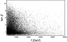
Figure 1: Prediction of $f$ and $\tan\beta$ in the C2HDM.

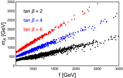
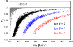
Figure 2: Prediction of $m_{A}$ as a function of $f$ in the C2HDM for $\tan\beta=2$, 4 and 6.

Figure 3: Comparison in the correlation of $m_{A}$ versus $\kappa_{V}$ between the C2HDM and MSSM for $\tan\beta=2,4$ and 6 in the former and all values of $\tan\beta$ in the latter.

2. Alignment with Delayed Decoupling – In addition to Higgs masses, further physics observables that can be used to compare the C2HDM to the MSSM are, e.g., Higgs cross sections and branching ratios. A convenient way to exploit the latter in order to extract the model parameters of potential new physics in the Higgs sector is to recast them in the language of the so called $\kappa_{i}$ ‘modifiers’ of Ref. LHCHiggsCrossSectionWorkingGroup:2012nn , wherein any of the latter is nothing but a coupling of the SM-like Higgs boson discovered at the LHC to known fermions ($i=b,t,\tau$) and bosons ($i=g,\gamma,Z,W^{\pm}$) normalised to the corresponding SM prediction. In order to compare the C2HDM and MSSM in this framework, we turn now to the case of $\kappa_{V}$ ($V=Z,W^{\pm}$), this being the most precisely known of all $\kappa_{i}$’s. In the C2HDM the $hVV$ ($V=Z,W^{\pm}$) coupling, normalised to the SM prediction, is given by

$$\kappa_{V}=\left(1-\frac{\xi}{2}\right)\cos\theta,\quad\xi\equiv\frac{v_{\textrm{SM}}^{2}}{f^{2}},$$ (13)

where $\theta\to 0$ with $f\to\infty$ corresponds to the alignment limit, i.e., the couplings of $h$ to SM particles become the same as those of the SM Higgs boson at tree level. Fig. 3 shows that the (near) alignment limit ($\kappa_{V}\sim 1$) is reached at large Higgs boson masses (exemplified here by the CP-odd one) in both the C2HDM and MSSM. However, a remarkable difference is seen in this behaviour. In the MSSM, $\kappa_{V}$ (see Djouadi for its expression) very quickly reaches 1. In contrast, in the C2HDM, $\kappa_{V}$ approaches 1 slowly (and the velocity at which this happens depends strongly on $\tan\beta$). This delayed decoupling is mainly driven by the negative ${\cal O}(\xi)$ corrections which are typical of composite Higgs models, as seen in Eq. (13), combined with the fact that the slopes seen in Fig. 3 for the C2HDM exhibit the dependence of $m_{A}$ from $f$ illustrated in Fig. 3, which allows a different and wider spread of $\kappa_{V}$ values away from 1 with respect to the MSSM. We note that values of $\kappa_{V}\gtrsim 0.9$ are currently compatible with LHC data at 1$\sigma$ level Khachatryan:2016vau . Therefore, if a large deviation in the $hVV$ coupling from the SM prediction will be restricted by future experiments, it will imply a larger Compositeness scale in the C2HDM. Conversely, if such a deviation will instead be established and no heavy Higgs state below 400 GeV or so will be seen, the MSSM may be ruled out and the C2HDM could explain the data. Therefore, either way, by combining the measured value of $\kappa_{V}$ to that of an extracted or excluded $m_{A}$, one may be able to discriminate the C2HDM from the MSSM.

3. Mass Hierarchy Amongst Heavy Higgs States – Fig. 4 shows the mass differences $m_{H^{\pm}}-m_{A}$ and $m_{H}-m_{A}$ where $\tan\beta$ has been varied over all its possible values in our two reference models, as explained above. We find that (top frame), while $m_{H^{\pm}}$ and $m_{A}$ are very close in the C2HDM, within 5 GeV, larger mass differences between these two heavy Higgs bosons are allowed in the MSSM, particularly for smaller $m_{A}$, e.g., $m_{H^{\pm}}-m_{A}$ can reach $\approx 30$ GeV for $m_{A}=200$ GeV. Due to the particular structure of the scalar potential, the contribution of the fermionic sector cancels out in the mass splitting of $A$ and $H^{\pm}$ and only the gauge sector one survives. The latter can be approximated by $(m_{H^{\pm}}-m_{A})/m_{A}\simeq g^{\prime 2}\xi$, with $g^{\prime}$ the hypercharge gauge coupling. This represents a robust prediction of the model. Conversely, for $m_{H}-m_{A}$ (bottom frame), it is the other way around. With increasing $m_{A}$, starting from 300 GeV, the mass difference between the two heavy neutral Higgs bosons tends to be confined within 5 GeV or so for the MSSM while in the C2HDM this can range from $-40$ GeV (at moderate $m_{A}$) to $+40$ GeV (for larger $m_{A}$). The mass splitting is not strictly determined as in the $m_{H^{\pm}}-m_{A}$ case but can be, nevertheless, estimated by $(m_{H}-m_{A})/m_{A}\simeq c\,\xi$ with $c$ being an order 0.1 coefficient encoding the dependence on the fermionic parameters of the strong sector. The $\xi$ factor, appearing in the formulas of the mass splittings, reproduces the expected mass degeneracy among $A,H$ and $H^{\pm}$ in the large $f$ regime. Interestingly then, the hierarchy amongst $m_{H^{\pm}}$, $m_{A}$ and $m_{H}$ may enable one to distinguish between the two scenarios as (recalling that three-body decays via off-shell gauge bosons are possible) establishing $H^{\pm}\to W^{\pm*}A$ would point to the MSSM while extracting $H\to Z^{*}A$ or $A\to Z^{*}H$ would favour the C2HDM.

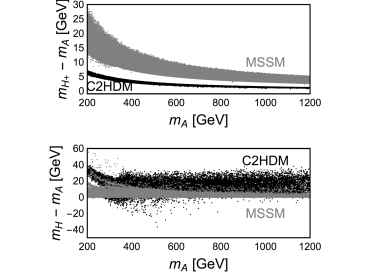
Figure 4: Comparison in the correlation of $m_{A}$ versus $m_{H^{\pm}}-m_{A}$ (top) and $m_{H}-m_{A}$ (bottom) between the C2HDM and MSSM for all values of $\tan\beta$ in both scenarios.

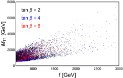
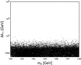
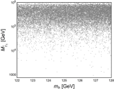
Figure 5: Correlation of $M_{T_{1}}$ versus $f$ in the C2HDM for $\tan\beta=2$, 4 and 6.

Figure 6: Left: Correlation of $m_{h}$ versus $M_{T_{1}}$, the mass of the lightest 2/3 fermionic partner in the C2HDM. Right: Correlation of $m_{h}$ versus $M_{{\tilde{t}}_{1}}$, the mass of the lightest stop in the MSSM. Plots are for all values of $\tan\beta$ in both scenarios.

4. Lower-lying Top Quark Partners – Needless to say, just like the Higgs masses, the composite top quark partner masses are strongly correlated to $f$. In Fig. 6, we show, e.g., the correlation between $f$ and the lightest top partner mass $M_{T_{1}}$. Here, we can see that the $\tan\beta$ dependence is rather unimportant. In particular, we find that typically a minimum $M_{T_{1}}$ is required and such a lower limit gets higher as $f$ increases. For a given $f$, the minimum allowed value of $M_{T_{1}}$ is $\sim f$, and it is strictly determined by the reconstruction of the top mass from the parameters of the strong sector. This behaviour agrees with well-established results in minimal composite Higgs models 4dchm ; Panico:2012uw . A distinctive feature between the C2HDM and MSSM in connection with the heavy (s)top sector is the fact that the measured value of $m_{h}\sim 125$ GeV requires a (fermionic) top quark partner in the C2HDM with a mass significantly lower than the (scalar) top quark partner in the MSSM. The lightest $2/3$ fermion partner in the C2HDM is then potentially accessible at the LHC whatever the actual $m_{h}$ value, see Fig. 6. This is much unlike the MSSM, for which the stop mass is, over the majority of the parameter space, far beyond the reach of the LHC Djouadi:2013vqa ; Djouadi:2015jea . In essence, present knowledge of the Higgs sector implies that the C2HDM is more readily accessible in the top partner sector than the MSSM. It is worth noticing that this result relies on the particular structure of the superpotential of the MSSM and could be modified in other supersymmetric scenarios. An interesting example is provided by the Next-to-MSSM (NMSSM) in which the presence of a SM-singlet chiral superfield allows for more freedom in the calculation of the Higgs mass. This implies that the dependence of $m_{h}$ on the lightest stop mass is relaxed with respect to the MSSM so that $M_{\tilde{t}_{1}}$ could be lowered down to the TeV region. Likewise, Compositeness models with different global symmetries and/or fermionic representations may result in different Higgs and/or top partner spectra.

Conclusions – We have calculated the mass and coupling spectra of a C2HDM based on the global symmetry breaking of $SO(6)\to SO(4)\times SO(2)$, as all these physical quantities are predicted by the dynamics of such a strong sector. In particular, we have focused on the differences between predictions given in the C2HDM and MSSM, both of which provide a 2HDM as a low energy effective theory of EWSB, specifically, an A2HDM in the case of Compositeness and a Type-II 2HDM in the case of Supersymmetry. We found remarkable differences between the C2HDM and MSSM. Namely, (i) $\tan\beta$ is predicted in the C2HDM, whereas this parameter is arbitrary in the MSSM, (ii) all Higgs boson masses are also predicted within the C2HDM for a given value of $f$ (unlike in the MSSM), (iii) the speed of decoupling of the extra Higgs bosons in the C2HDM is much slower than in the MSSM, (iv) different size mass splittings amongst the extra neutral Higgs states are predicted in the C2HDM with respect to the MSSM, so that establishing different Higgs-to-Higgs plus gauge boson decays at the LHC could potentially distinguish between the two scenarios, (v) the mass of the lightest (fermionic) top quark partner in the C2HDM can be much smaller than the lightest (scalar) stop mass in the MSSM. Remarkably, all these aspects are amenable to investigation at current LHC experiments in the years to come, so that a clear potential exists in the foreseeable future to disentangle two possible solutions of the SM hierarchy problem, i.e., Compositeness and Supersymmetry.

Acknowledgements – The work of SM is supported in part by the NExT Institute and the STFC Consolidated Grant ST/L000296/1. We all thank Sven Heinemeyer, Suchita Kulkarni and Andrea Tesi for illuminating discussions.

References

- (1) S. De Curtis, L. Delle Rose, S. Moretti, A. Tesi and K. Yagyu, in preparation.
- (2) A. Djouadi, Phys. Rept. 459 (2008) 1.
- (3) D. B. Kaplan and H. Georgi, Phys. Lett. B 136 (1984) 183.
- (4) S. De Curtis, M. Redi and A. Tesi, JHEP 1204 (2012) 042.
- (5) J. Mrazek, A. Pomarol, R. Rattazzi, M. Redi, J. Serra and A. Wulzer, Nucl. Phys. B 853 (2011) 1.
- (6) A. Pich and P. Tuzon, Phys. Rev. D 80 (2009) 091702.
- (7) G. C. Branco, P. M. Ferreira, L. Lavoura, M. N. Rebelo, M. Sher and J. P. Silva, Phys. Rept. 516 (2012) 1.
- (8) P. Bechtle, O. Brein, S. Heinemeyer, O. St l, T. Stefaniak, G. Weiglein and K. E. Williams, Eur. Phys. J. C 74 (2014) no.3, 2693
- (9) P. Bechtle, S. Heinemeyer, O. St l, T. Stefaniak and G. Weiglein, Eur. Phys. J. C 74 (2014) no.2, 2711
- (10) S. Heinemeyer, W. Hollik and G. Weiglein, Comput. Phys. Commun. 124 (2000) 76.
- (11) T. Hahn, S. Heinemeyer, W. Hollik, H. Rzehak and G. Weiglein, Phys. Rev. Lett. 112 (2014) 141801.
- (12) E. Bagnaschi et al., LHCHXSWG-2015-002.
- (13) G. Panico, M. Redi, A. Tesi and A. Wulzer, JHEP 1303 (2013) 051.
- (14) S. Davidson and H. E. Haber, Phys. Rev. D 72 (2005) 035004 [Erratum: Phys. Rev. D 72 (2005) 099902].
- (15) H. E. Haber and D. O’Neil, Phys. Rev. D 74 (2006) 015018 [Erratum: Phys. Rev. D 74 (2006) 059905].
- (16) H. E. Haber and D. O’Neil, Phys. Rev. D 83 (2011) 055017.
- (17) A. David et al. [LHC Higgs Cross Section Working Group], arXiv:1209.0040 [hep-ph].
- (18) G. Aad et al. [ATLAS and CMS Collaborations], JHEP 1608 (2016) 045.
- (19) A. Djouadi and J. Quevillon, JHEP 1310 (2013) 028.
- (20) A. Djouadi, L. Maiani, A. Polosa, J. Quevillon and V. Riquer, JHEP 1506 (2015) 168.