Mott transition with Holographic Spectral function

Abstract

We show that the Mott transition can be realized in a holographic model of a fermion with bulk mass, $m$, and a dipole interaction of coupling strength $p$. The phase diagram contains gapless, pseudo-gap and gapped phases and the first one can be further divided into four sub-classes. We compare the spectral densities of our holographic model with the Dynamical Mean Field Theory (DMFT) results for Hubbard model as well as the experimental data of Vanadium Oxide materials. Interestingly, single-site and cluster DMFT results of Hubbard model share some similarities with the holographic model of different parameters, although the spectral functions are quite different due to the asymmetry in the holography part. The theory can fit the X-ray absorption spectrum (XAS) data quite well, but once the theory parameters are fixed with the former it can fit the photoelectric emission spectrum (PES) data only if we symmetrize the spectral function.

1 Introduction

The Mott transition, the interaction induced Metal-Insulator transition (MIT)MOTT:1968aa , is a challenging subject and quantitative understanding of such phenomena is a necessary virtue of any successful theory of for strongly interacting system (SIS). The physics of Mott transition is usually discussed using the Hubbard model $H=-t(\sum c^{\dagger}_{i\sigma}c_{j\sigma}+H.c.)+U\sum n_{i\uparrow}n_{i\downarrow},$ which capture the competition between the hopping and the on-site repulsion. However, for 2+1 and higher dimension, it has not been solved for more than half century.

Holographic method has been developed as a theory of SIS Zaanen:2015oix ; Hartnoll:2016apf , and it is natural to ask whether it can describe the Mott transition in terms of fermion spectral function. However, finding the exact gravity dual of a given theory is extremely difficult if possible at all. Furthermore, Hubbard model is just one simple model that captures some essence of the Mott transition, so finding an exact dual of such model is not essential either. In this situation, instead of trying to find the dual of the Hubbard model, it would be more sensible to find a holographic model that can achieve the same physics.

There has been much effort on holographic fermion spectral function starting from sslee . The marginal non-Fermi liquids in holography is established Liu:2009dm ; Faulkner:2009wj ; Faulkner:2011tm ; Faulkner:2013bna . On the one hand, holographic gap generation was discussed in Edalati:2010ge ; Edalati:2010ww ; Vanacore:2014hka ; Vanacore:2015poa ; Ling:2014bda using the dipole term or Pauli term

$$p\bar{\psi}F^{\mu\nu}\sigma_{\mu\nu}\psi.$$ (1)

On the other hand, the emergence of free fermion-like point at the bulk mass 1/2 and the nearby Fermi-liquid-like phase was found in Cubrovic:2009ye ; Cubrovic:2010bf ; Medvedyeva:2013rpa . Putting these together, we might expect that Mott transition can be handily described in holography and Hubbard model can be replaced in terms of easily calculable theory. However, the Hubbard model is a free fermion at $U=0$, while the holographic theory is strongly interacting even at the absence of the gap generating term, which is a generic property of a holographic theory. Therefore it is not clear how similar and different are the two theories and we need to see the detail to decide the usefulness of the new theory.

In this paper we study the phase structure of the holographic fermion model with the bulk mass term and a gap generating interaction given by (1). We find that rather surprisingly, for a fixed bulk mass, the model can describe a transition between the gapless and gapful phases only when we restrict the bulk mass below the critical mass $m_{c}\simeq 0.35$ . We also find that there is a rather large region of pseudo-gap, a phase where the density of state is depleted near the Fermi sea. The phase diagram is richer than expected since the gapless phase can be further divided into four subclasses: the bad metal phases with and without shoulder peaks and the half-metal phase with a gap between the shoulder peak and the central peak apart from the Fermi-liquid like phase first discovered in Cubrovic:2009ye . The presence of half-metal is a surprise at first, but it can be understood as the proximity effect of the ’free fermion Wall’ sitting at $m=1/2$ line in the phase diagram.

It turns out that there is a phenomenologically important difference between the holographic model discussed here and the Hubbard model: the spectral function of the Hubbard model is symmetric at the half filling, while that in the present holographic model is highly asymmetric for any non-vanishing charge density without which gap is not generated. Obviously, the real systems are in between.

With such differences understood, it is now meaningful to seek the commonness and similarity between the different models which realizes Mott transition. Since Hubbard model contains essentially one parameter, $U/t$, and the holographic model has two parameters $m$ and $p$, we need to take a path in the phase diagram, which we call embedding. We will see that there are two common features: i) transfer of the degree of freedom from the central to shoulder peaks, ii) smoothness of the transition. Our calculation shows that all the transitions are smooth crossover. Therefore one may wonder why we call a regime as a phase. However, gap and gapless is certainly very different although smoothly connected through the pseudo-gap region, which had been classified as a phase of SIS. We suggest that such smooth transition with intermediate zone is a general character of SIS. For the second feature, we will see that there are two paths in gap creation: in one path, the central peak begins to be reduced in height from the beginning and the gap is created by such reducing process. In the middle, pseudo-gap appears in the middle. In the other path, the central peak remains sharp but its weight and width is getting thinner. For the second path or embedding, the gap creation is done by such thinning process. It is really surprising that in the DMFT study of Hubbard model such two different paths for opening the gap were achieved by different approximation scheme. One is called single-site DMFT and the other is cluster DMFT. It is a bit mysterious how such different features which would be expected from different models could be obtained in the same model in both cases: in DMFT as different approximation schemes and in the holographic model as different parameter regimes.

Finally we tested our model with the experiment using the Vanadium oxide data. It turned out that the X-ray absorption Spectrum (XAS) data can be fit by our theory but the photoelectric emission (PES) data can not be unless spectral functions are symmetrized by hand.

2 Spectral function

2.1 Setup and review

We start from the fermion action in the dual spacetime with non-minimal dipole interaction,

$$S_{D}=\int d^{4}x\sqrt{-g}\bar{\psi}\left(\Gamma^{M}{\cal D}_{M}-m-ip\,\Gamma^{MN}F_{MN}\right)\psi+S_{\text{bd}},$$ (2)

where the subscript $D$ denotes the Dirac fermion and the covariant derivative is

$${\cal D}_{M}=\partial_{M}+\frac{1}{4}\omega_{abM}\Gamma^{ab}-iqA_{M}.$$ (3)

For fermions, the equation of motions are first order and we can not fix the values of all the component at the boundary, which make it necessary to introduce ‘Gibbons-Hawking term’ $S_{\text{bd}}$ to guarantee the equation of motion which defined as

$$-iS_{\text{bd}}=\pm\frac{1}{2}\int d^{d}x\sqrt{h}\bar{\psi}\psi=\pm\frac{1}{2}\int d^{d}x\sqrt{h}(\bar{\psi}_{-}\psi_{+}+\bar{\psi}_{+}\psi_{-}),$$ (4)

where $h=-gg^{rr}$, $\psi_{\pm}$ are the spin-up and down components of the bulk spinors. The sign is to be chosen such that, when we fix the value of $\psi_{+}$ at the boundary, $\delta S_{bd}$ cancel the terms including $\delta{\psi}_{-}$ that comes from the total derivative of $\delta S_{D}$. Similar story is true when we fix $\psi_{-}$. The former defines the standard quantization and the latter does the alternative quantization. The background solution we will use is Reisner-Nordstrom black hole in asymptotic $AdS_{4}$ spacetime,

$$ds^{2} =-\frac{r^{2}f(r)}{L^{2}}dt^{2}+\frac{L^{2}}{r^{2}f(r)}dr^{2}+\frac{r^{2}}{L^{2}}d\vec{x}^{2}$$ (5)

$$f(r) =1+\frac{Q^{2}}{r^{4}}-\frac{M}{r^{3}},~{}~{}~{}~{}~{}A=\mu\left(1-\frac{r_{0}}{r}\right),$$ (6)

where $L$ is AdS radius, $r_{0}$ is the radius of the black hole and $Q=r_{0}\,\mu,M=r_{0}(r_{0}^{2}+\mu^{2}).$ The temperature of the boundary theory is given by $T={f^{\prime}(r_{0})}/{4\pi}$ and it can be solved for $r_{0}$ to give $r_{0}=(2\pi T+\sqrt{(2\pi T)^{2}+3\mu^{2}})/3$.

Following Liu:2009dm , we now introduce $\phi_{\pm}$ by

$$\psi_{\pm}={(-gg^{rr})}^{-\frac{1}{4}}\phi_{\pm},\quad\phi_{\pm}=\left(\begin{array}[]{ccc}y_{\pm}\\ z_{\pm}\\ \end{array}\right),$$ (9)

after Fourier transformation. Then the equations of motion become Liu:2009dm ,

$$\sqrt{\frac{g_{xx}}{g_{rr}}}z_{+}^{\prime}(r)-mL\,\sqrt{g_{xx}}z_{+}(r)+i[u(r)+k-p\sqrt{g_{xx}}A_{t}^{\prime}(r)]y_{-}(r) =0$$ (10)

$$\sqrt{\frac{g_{xx}}{g_{rr}}}y_{-}^{\prime}(r)+mL\,\sqrt{g_{xx}}y_{-}(r)+i[u(r)-k+p\sqrt{g_{xx}}A_{t}^{\prime}(r)]z_{+}(r) =0,$$ (11)

where $u(r)=\sqrt{\frac{g_{xx}}{-g_{tt}}}(\omega+qA_{t}(r)).$ Here, the momentum is along $x$ direction. The corresponding equations for $y_{+},z_{-}$ are obtained from the above by $(A_{t},\omega)\to(-A_{t},-\omega)$.

At the boundary region($r\rightarrow\infty$), the geometry becomes $AdS_{4}$ and the equations of motion (11) have analytic solution as

$$z_{+} =A_{1}\chi_{1}(r)+B_{1}\chi_{2}(r),\quad y_{-} =C_{1}\chi_{3}(r)+D_{1}\chi_{4}(r),$$ (12)

$$y_{+} =A_{2}\chi_{1}(r)+B_{2}\chi_{2}(r),\quad z_{-} =C_{2}\chi_{3}(r)+D_{2}\chi_{4}(r),$$ (13)

where

$$\chi_{1}(r) = r^{m}\,_{0}F_{1}\left(\frac{1}{2}-m;-\frac{W}{4r^{2}}\right),\quad\chi_{2}(r)=r^{-m-1}\,_{0}F_{1}\left(m+\frac{3}{2};-\frac{W}{4r^{2}}\right),$$

$$\chi_{3}(r) = r^{m-1}\,_{0}F_{1}\left(\frac{3}{2}-m;-\frac{W}{4r^{2}}\right),\quad\chi_{4}(r)=r^{-m}\,_{0}F_{1}\left(m+\frac{1}{2};-\frac{W}{4r^{2}}\right),$$ (14)

with $W=(\omega+q\,\mu)^{2}-k^{2}$. The asymptotic behaviors of (14) are manifest if we notice ${}_{0}F_{1}\to 1$ in $r\to\infty$. The equation of motion produces the relations of coefficients:

$$C_{1}=\frac{iA_{1}\left(k-(\omega+q\,\mu)\right)}{2m-1},~{}~{}~{}~{}~{}B_{1}=\frac{iD_{1}\left(k+(\omega+q\,\mu)\right)}{2m+1},$$ (15)

$$C_{2}=\frac{iA_{2}\left(k+(\omega+q\,\mu)\right)}{2m-1},~{}~{}~{}~{}~{}B_{2}=\frac{iD_{2}\left(k-(\omega+q\,\mu)\right)}{2m+1}.$$ (16)

Here, we made an abbreviation for $mL$ with $m$, which we will restore at the end.

The boundary term in Eq.(4) becomes

$$-iS_{\text{bd}}= y_{-}z_{+}-y_{+}z_{-}=(A_{1}D_{1}-A_{2}D_{2})+\sum_{\pm}E_{\pm}r^{\pm 2m-1}+E_{2}r^{-2},$$ (17)

using the asymptotic behavior of wave functions $\chi_{i}$. Here, $E_{\pm}$ and $E_{2}$ are functions of the coefficients of $\chi_{i}$. A few remarks are in order. First, for $m>1/2$, the second term($E_{\pm}$) dominates but it can be cancelled by counter terms Ammon:2010pg , which do not contribute any finite terms to the effective action. Second, in the standard quantization where we fix $\psi_{+}$ at the boundary, $A$’s are the source terms. While in the alternative quantizaton where we fix $\psi_{-}$ at the boundary, $D_{i}$ is taken to be the source. Therefore, if variables with index 1 and those with index 2 are separable, the retarded Green’s function in standard quantization, is given by

$${\cal G}=\text{diag}\bigg{(}i\frac{D_{1}}{A_{1}},-i\frac{D_{2}}{A_{2}}\bigg{)}\equiv\text{diag}(G_{+}^{R},G_{-}^{R}),\quad m>0,$$ (18)

while that in alternative quantization is given by

$${\tilde{\cal G}}=\text{diag}\bigg{(}i\frac{A_{1}}{D_{1}},-i\frac{A_{2}}{D_{2}}\bigg{)} \equiv\text{diag}(\tilde{G}_{+}^{R},\tilde{G}_{-}^{R})$$ (19)

$$=-\text{diag}(1/G_{+}^{R},1/G_{-}^{R}),\quad m>0.$$ (20)

Since $G_{R}$ for $m<0$ case, can be also obtained by $G_{R}\to-1/G_{R}$, ${\tilde{G}_{R}}$, the Green function for the alternative quantization for $m>0$, is the same as that for $-m$ in the standard quantization:

$${\tilde{G}_{\pm}^{R}(\omega,k;m)}=-1/G_{\pm}^{R}(\omega,k;m)=G_{\mp}^{R}(\omega,k;-m).$$ (21)

Introducing the $\xi_{\pm}$ by

$$\xi_{+}=i\frac{y_{-}}{z_{+}},\hbox{ and }\quad\xi_{-}=-i\frac{z_{-}}{y_{+}},$$ (22)

the equations of motion Eqs.(11) can be recast into two independent equations for $\xi_{\pm}$:

$$\sqrt{\frac{g_{xx}}{g_{rr}}}\xi_{\pm}^{\prime}=-2m\sqrt{g_{xx}}\xi_{\pm}+[u(r)+p\sqrt{g_{xx}}A_{t}^{\prime}(r)\mp k]+[u(r)-p\sqrt{g_{xx}}A_{t}^{\prime}(r)\pm k]\xi_{\pm}^{2}.$$ (23)

and the Green functions for $m<1/2$ can be written as

$$G^{R}_{\pm}(\omega,k)=\lim_{r\to\infty}r^{2m}\xi_{\pm}(r,\omega,k).$$ (24)

Notice that two components of the Green function are not independent: $G^{R}_{-}(\omega,k)=G^{R}_{+}(\omega,-k).$ The spectral function is defined as the imaginary part of the Green function. There are two of them ${\rm Im}[G^{R}_{+}]$ and ${\rm Im}[G^{R}_{-}]$ and we can define the spectral function for each of them:

$$A_{\pm}(\omega,k)={\rm Im}[G^{R}_{\pm}(\omega,k)].$$ (25)

There is an issue on the finiteness of the spectrum: it was pointed out Gursoy:2011gz that the high frequency behavior of the spectral function diverges like $\omega^{2m}$ so that the sum of the degree of freedom over frequency is infinite if $m$ is positive. Therefore we need to take the negative bulk mass only in the standard quantization. For the ease of discussion we want to maintain the positivity of the mass which can be done simply by going to the alternative quantization. Even in this case spectral function is $\sim\omega^{-2m}$ which does not decay fast enough to guarantee the finite integration. The sum rule can be still an issue and we do not treat this problem here. Summarizing, we work in alternative quantization with positive mass and we treat the fermion as a probe and do not consider its back reaction.

2.2 Non-relativistic system in terms of relativistic formulation

Now how do we define the physical spectral function that can be compared with experimental data? For relativistic system like Dirac or Weyl semi-metal, it is natural to define it as the traced object which is the sum of the two: ${\rm Im}[G^{R}_{+}+G^{R}_{-}]$. One expect that the chemical potential is small so that the Fermi level is near the Dirac point. In fact we have a few experiences that such Dirac material with small Fermi sea can be well described by the RN black hole physics Seo:2016vks ; Seo:2017oyh ; Seo:2017yux .

However, if we want to describe a non-relativistic system, the problem is more subtle as we describe below. Notice that in the presence of chemical potential, the dispersion relation near the Fermi sea is linear so that we expect that dynamical aspect are not much different between relativistic and non-relativistic cases. However, the relativistic spectrum is a double of non-relativistic case in the former handle the negative and positive frequency at equal footing. Therefore when compare the two, half of the relativistic spectrum should be projected out. Indeed, the relativistic case has a serious problem in describing real non-relativistic system because it has unphysical spectrum far below fermi surface. This can be seen by considering weakly interacting system with chemical potential. Notice that the fermi level is defined by $G_{-}^{-1}\sim\omega+\mu-k-\Sigma=0$ with $\omega=0$. For a weakly interacting system, the self energy $\Sigma\simeq 0$, then $k_{c}$, the momentum at which we consider the spectral function can be taken as $k_{c}=\mu:=k_{F}$. Then the spectrum or the pole of the $G_{+}^{-1}$ would be at $\omega=-2\mu$, because $G_{+}^{-1}\sim\omega+\mu+k_{c}-\Sigma=0$. For large chemical potential the spectral function has high peak deep under the Fermi sea, which is certainly unphysical.

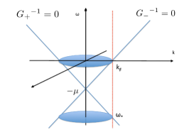
(a) Relativistic Spectrum(RS)

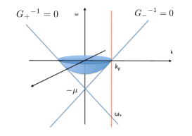
(b) NRS approximated by RS

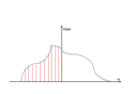
(c) Half filling

Figure 1: (a)spectrum in relativistic formulation. (b) Unphysical spectrum appear in the $G_{+}$ in hole sector when we approximate the non-relativistic spectrum (NRS) in terms of the relativistic theory near Fermi level. To elliminate such pole we define the spectral function by eliminating the spectrum deep under the Fermi sea: $\omega<-\mu$. (c) Definition of half filling.

See the figure 1, where the spectral function as function of $\omega$ along the $k_{c}=k_{F}$ line has two peaks: one at the fermi surface and the other at the $\omega=\omega_{*}=-2\mu$, deep in the fermi sea. Such feature is attributed to the relativistic formulation of the fermion and it continues to exist for strongly interacting system. When we describe a non-relativistic system in terms of relativistic fermions, we have to exclude such spectrum. Therefore we identify our spectral function as ${\rm Im}[G^{R}_{-}]$ rather than the traced one.

$$A(\omega,k_{c})=A_{-}={\rm Im}[G^{R}_{-}(\omega,k_{c})]$$ (26)

This is fine for practical purpose where we set $k$ non zero only along x-direction but it is not a rigorous definition, because in more than 1+1 dimension $G_{+}$ and $G_{-}$ are not separable, as the lightcone structure in figure 1 suggests. More proper way to state it is to discard the spectrum under $\omega<-\mu$ if $\mu>>T$.

2.3 definition of the half filling in the absence of the lattice

In most practical calculation of holography, one does not encode the presence of the lattice. However, the starting point of Mott transition is the having half filled band which is certainly band conductor, which should become insulator under the growth of the coupling strength. Therefore we need to ask what is the definition of the the half filling when we do not encode the lattice. One may think this is not a serous question in holography since generic phase of fermion in the absence of extra interaction is a bad metal and we have at least one a gap generating interaction. However, it is rather confusing in understanding the definition of the doping which is necessary to calculate physical quantity in terms of the doping rate. Here we propose that the system is half filled if the Fermi level $\omega=0$ divide the density of state by half, namely if the area under the density of state (DOS) graph is divided into two equal areas by $\omega=0$. See figure 1(c). If we denote the general density by $Q$ and the half filling density by $Q_{0}$, then the doping rate $x$ is expressed by $x={(Q-Q_{0})}/{Q_{0}}.$

3 The phases of holographic fermion

We study the phases diagram of the model given by Eq. (2) as function of $p$ and $m$. There are two self evident phases: gapless, gapped phases. The pseudo-gap appears as an interpolating zone of these two phases. The phase diagram is richer than expected, because the gapless phase can be subdivided into four subclasses: Fermi liquid like (FL), bad metal(BM), bad metal prime(BM’) and half-metal(hM) phases.

The most typical phase of the gapless phase is bad metal phase. Since $A(\omega,k)\sim\omega^{-2m}$, it is not well localized near Fermi surface (FS). The peak at the free fermion point $(p,m)=(0,1/2)$ is singularly sharp. For the continuity of the phase diagram, we have to install a Fermi liquid like phase near that point and we take the phase boundary value to be $m\sim 0.35$. However this phase can not be a real Fermi liquid in two aspects: i) the central peak is not really localized and decays too slowly as mentioned above. ii) the width of the central peak does not follow $\Gamma\sim T^{2}$ law. Instead, we find that they follow $\Gamma\sim T$ law for small chemical potential $\mu/T\ll 1$. The reason we call it Fermi liquid like phase is due to the sharp linear dispersion relation $\omega+\mu=\pm k$. Also for large chemical potential $\mu/T\gg 1$, we find the half width of the central peak $\Gamma\sim T^{\alpha}$ with $\alpha\simeq 2$ so that it resembles the true Fermi liquid. See the figure 4.

The reason of free fermion point at $(p,m)=(0,1/2)$ is well understood Cubrovic:2009ye ; Faulkner:2009wj . $\psi$ is the dual of the operator with dimension $\Delta=d/2-m$ which is dimension of free fermion when $m=1/2$ so that the fermion with $m=1/2$ in alternate quantization is dual to the free fermion. Along the $m=1/2$ line in the phase diagram, the spectral function is also sharp although the spectrum can be more diversified. We call that line as ‘free fermion wall’. The bad metal prime is the bad metal with shoulder peak(s). See Figure 2(d) and (b). The half metal is the bad metal prime with a gap between the central peak and the shoulder peak. See Figure 2(c).

Since the transitions are smooth everywhere, one may wonder whether we can classify the phases. However, it would be more strange if we say that SIS has just one phase since even the gap and gapless phases are smoothly connected. With this understanding, the phase boundary naturally depends on the choice of the criterion: we choose the onset of pseudo-gap by $R=0.9$ where $R$ is the ratio of the spectral function at the central dent, $A(\omega=0,k_{c})$, to that at the Hubbard peak. Here $k_{c}=k_{F}$ if $k_{F}$ exists, otherwise it is the momentum at which one of the dispersion curve branch just touches the fermi level $\omega=0$ which happens at $m=0.35$. See figure 5(b). For the gapped phase we choose $R=0.01$.

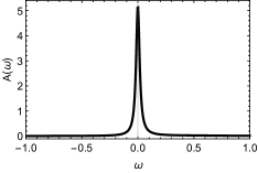
(a) Fermi liquid like (FL)

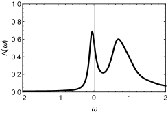
(b) bad metal prime (BM’)

(c) half-metal (hM)

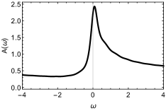
(d) bad metal (BM)

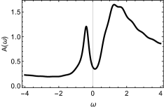
(e) pseudogap (PG)

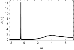
(f) gapped (G)

Figure 2: (a)-(f):Typical fermion phases. (a) FL with (p=0.5, m=0.45,$k_{c}=1.65$), (b) BM’ with shoulder (p=2, m=0.4, $k_{c}=2.30$), (c) hM (p=6, m=0.45, $k_{c}=2.48$), (d) BM without shoulder (p=0.5, m=0.1, $k_{c}=1.20$), (e) PG (p=2,m=0.1,$k_{c}=2.89$): notice the position of the $\omega=0$ compared with the BM’ phase in (b), (f) Gapped phase (p=6, m=0.15, $k_{c}=5.68$)

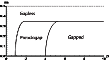
(a) Phase diagram

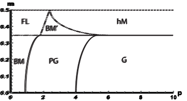
(b) Substructure in gapless phase

Figure 3: Phase diagram in $(p,m)$ space. (a) Three phases which are gapless, psuedo-gap and Gapped phases, appear and all transitions are smooth crossover. The gapless phase can be further divided into four subregions: Fermi liquid like (FL), bad metals (BM), bad metal prime (BM’), half metal (hM).

The result of the detailed study of phases are summarized by the phase diagram given in Figure 3. The dashed line along $m=0.5$ represents the free fermion wall, the FL phase is located at the upper-left corner and gapped phase is at the lower-right corner. All other phases are in between the two and can be understood as proximity and competition of the two phases. Notice also that the phase diagram is divided by the line of $m\simeq 0.35$: the lower half region is where gap-generation phenomena is observed as we expected from the presence of the dipole term. However, in the upper region, a new metallic phase appears instead of gapped one. We call it half-metal phase, because significant fraction of density of state is depleted from the quasi-particle peak near the Fermi level and moved to the shoulder region. The emergence of this new metallic phase in the strongly coupled system was unexpected. To understand its appearance, we study the effect of the dipole term on the spectral density near $m=0.5$. See figure 4.

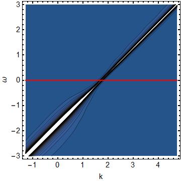
(a) $m=0.5,p=0$

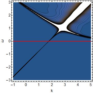
(b) $m=0.5,p=5$

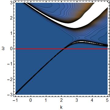
(c) $m=0.47,p=5$

Figure 4: Contour plot of spectral density for $m\sim 0.5$. Red line indicates the Fermi level. (a) At $p=0$, the degree of freedom follows the dispersion relation $\omega+\mu=k$, (b) At $p=5$, new branch of dispersion curve appears. (c) Lowering $m$ from 0.5, the spectral curves are reconnected to avoid the ’level crossing’.

It turns out that the peak along the dispersion curve $\omega+\mu=k$ exists along $m=0.5$ line although more and more degrees of freedom are depleted from the central peak and moved to the shoulder as we increase $p$ . We call the line $m=0.5$ ‘the free fermion wall’. One important effect of the dipole term is the creation of new band. See figure 4(b). As $p$ increases, it push down the new band below the Fermi level so that a gap is created and will be increased. The third effect of increasing $p$ is to make the new band sharper which means it keep transferring the spectral density from the central peak to the shoulder peak. This is similar to the effect of $U$ in the DMFT calculation of Hubbard model. Now lowering $m$ from 0.5, the spectral curves are reconnected to avoid the ’level crossing’. Consequently, the density profile moves from Figure 4(b) to (c).

We can now understand the the role of mass in creating the half-metal phase: increasing the $m$ pushes up the new band created by $p$ so that the band can cross the Fermi level. See figure 5. This effect competes with that of increasing $p$, but the effect of mass is stronger. For $m>0.35$ the new band always crosses Fermi sea and this is the mechanism of the hM phase. Notice that the new band touch the Fermi level at $m=0.35$ for all $p$.

(a) $m=0.25$

(b) $m=0.35$

(c) $m=0.45$

Figure 5: $m$-evolution at $p=6$ shows the origin of the the half-metalic phase: increasing the $m$ pushes up the new band, making the Fermi sea. Large $p$ is responsible for the sharpness of new band.

For small mass $m<0.35$, the dipole interaction leads to metal-insulator transition as $p$ increases. For $p>4$ and $m=0$, gap is dynamically generated as it was shown by Phillips et.al Edalati:2010ge . For larger mass, the gap generation requests slightly higher values of dipole strength. The pseudo-gap is nothing but the intermediate zone of this smooth transition, namely $0.8<p<4$ for $m=0$. Notice that in the phase diagram Figure 3, there is a rather large territory of PG.

Similarly, for $m>0.35$, the dipole term drives BM’ -hM transition because the new band always crosses the Fermi level. This is why strong dipole interaction leads to the half metal rather then a Mott insulator for in this regime. As $p$ increases the new band is narrowed and sharpened but it never disappears even at very large $p$. In the appendix, we study the evolution in m for fixed $p$ and evolution in $p$ for fixed $m$ in more detail.

The figure 6(a) shows that in the absence of the bulk mass, peak in the spectral density $k$-plot goes away very rapidly as soon as we turn on temperature. That is, quasi-particles are fragile at finite temperature, which is the character of non-Fermi liquids. On the other hand, if we turn on the mass, the Fermi surface peak becomes sharper as we can see in the Figure 6(b).

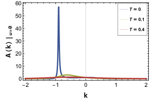
(a)

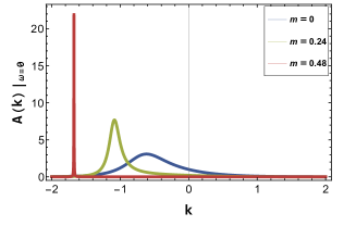
Figure 6: Role of mass in stabilizing the Fermi surface (FS): (a)Fast decay of FS for nonzero Temperature $T=0,0.1,0.4$ at $m=p=0$. (b) FS stabilized by bulk mass: $m=0,0.24,0.48$ at $T=0.1$ and $p=0$.

We can see the role of mass is the stabilizer of the quasi-particle nature in holographic matter. As $m\to 1/2$, such ‘quasi-particle stabilizing tendency’ increases singularly so that the system is a Fermi liquid like whatever is the strength of dipole term. In fact, the spectral function shows that the dispersion curve is straight line as if it is a free fermion. For applications to the realistic material, having such a dial to make the system Fermi liquid like in a limit is very useful because in the real experiments, one tunes the coupling by applying pressure or doping rate. In the presence of the dipole coupling whose role is to introduce a gap which break the conformal symmetry dynamically, there is no guarantee that the ’free fermion’ continues to exists. Our observation is that, nevertheless, such free fermion nature at $m=1/2$ persists in the presence of the dipole interaction regardless of its strength. We call it free fermion wall in $m$-$p$ phase diagram. We found that if $m>0.35$, metalic phase exist always as a consequence.

4 Comparison with other studies

4.1 Comparison with Hubbard Model

Usually a theoretical study for Mott transition has been done using the Hubbard model. Therefore it is inevitable to compare our result with the previous study of Hubbard model. We emphasize that our model is not the holographic dual of Hubbard model but a replacement of it for the Mott transition purpose. In fact the model studied here has a notable difference from the Hubbard model. First, $U=0$ in the latter is free fermion while $p=0$ in the former is not unless the bulk mass is fine tuned. Second, at the half filling, the Hubbard model has symmetric spectral function while the holographic theory does not. Third but most vividly, we have two parameters $m,p$ while the Hubbard model has only one, $U/t$. In order to compare our model to the result of Hubbard model, we have to restrict to an 1 dimensional subspace of the phase space, which we call embedding: namely, we associate a line in the parameter space $(p,m)$ in the holographic model that gives qualitatively the same spectral density. Any line connecting the free fermion point and the gapped phase can realize a Mott transition and define an embedding. Here we consider two simplest choices: the first one start from the free fermion point and reach at the gapped phase following a straight line

$$m+\alpha p=1/2,\quad p=U/t.$$ (27)

This defines a linear embedding given in Figure 7. The second starts from a point in the ’free fermion wall’, the line $m=1/2$, and rapidly goes down to small bulk mass regime and and turn there to reach the gapped regime following a curve

$$p=\beta(\frac{1}{2m}+1),\hbox{ with }\beta=constant.$$ (28)

We call it ’hyperbolic embedding’ and it is the red line in Figure 7.

There is no deep reason why we choose these two but it turns out to be of some interests. The linear embedding i) has central and shoulder peak structure ii) does not have pseudo-gap, and iii) as we increase the coupling $p$ (iii) the degree of freedom transfer from central peak to shoulder peak so that the central peak becomes thinner and thinner until gap is created. These three are the characteristic property of the single site DMFT result for Hubbard modelRevModPhys.68.13 . However, the holographic model has too much asymmetry in spectral function so that the and three peak structure which is one of the property of single site DMFT is not manifest since one of the shoulder is too weak. See Figure 8 (a) and (b).

The second embedding has pseudo-gap without central-peaks which is analogous to cluster DMFT results zhang2007pseudogap . The ‘transfer’ of the spectral density from the quasi-particle peak to the Hubbard side peaks are common to both embeddings. The apparent similarity between the two should be coming due to sharing the Mott transition. However, due to the large asymmetry again, the detail is different. The comparison of 2-site DMFT and its holographic analogue, the hyperbolic embedding, is given in figure 9 with $\beta=0.5$.

It is rather surprising that two different approximation scheme of DMFT for the same model behave as if they are different models and yet the holography can accommodate them with different parameter regime. Since we are comparing different theories, the similarity is overall one and they are different in detail. The difference in gap creation is worthwhile to emphasize. The single site DMFT RevModPhys.68.13 shows that the gap creation is ‘sudden’ since it is created with a finite size. On the other hand, linear embedding opens gap starting with zero size.

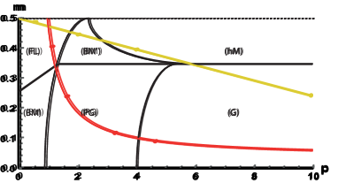
Figure 7: Phase diagram with two class of embeddings: Linear embedding mimics single site DMFT and the Hyperbolic one resembles two site DMFT. $\alpha,\beta$ in eq. (4.2) and (4.4) are $1/40$ and $1/20$ respectively.

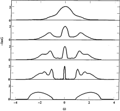
(a) single site DMFT result

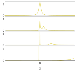
(b) Linear embedding

Figure 8: Comparision of DMFT results and Linear embedding. (a) Hubbard model in single site DMFT. The figure is from RevModPhys.68.13 . (b) Evolution of of Linear embedding. Transfer of DOS, persistence of central peaks till the gap formation are common with DMFT. But due to the heavy asymmetry in spectral function, the three peak structure of single site DMFT is not manifest here. $\alpha\simeq 1/40$.

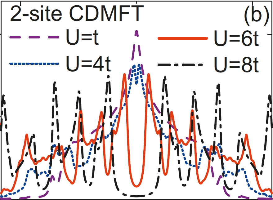
(a) 2-site DMFT result

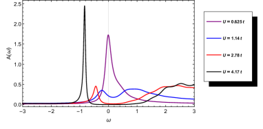
(b) a hyperbolic embedding

Figure 9: Comparision of cluster DMFT results: (a) Hubbard model in 2-site DMFT. The figure is from zhang2007pseudogap . (b) Evolution along the hyperbolic embedding in holographic model. Appearance of the pseudo-gap resembles cluster DMFT, but here again, due to the large asymmetry, the details look different.

4.2 Comparing with experiment

The ultimate test of a physical model is the capability of its explaining the data. Here we take Vanadium Oxides data and see how the theory fits data. It turns out that the X-ray absorpsion spectroscopy data for SrVO₃ (red circles and diamonds) sekiyama2002genuine and Ca_0.9Sr_0.1VO₃ (blue boxes and triangles) inoue1995systematic can be well fit with our theory. However the Photoemission (PES) data can not. The parameters taken to fit the XAS data create too much asymmetry in spectral function so that unless we symmetrize by hand, we do not have a room to accommodate the PES data. We do not have a good reason to perform such symmetrization although in some literature it is practiced norman1998phenomenology ; lee2007abrupt ; kondo2009competition . Once symmetrized, can the data can be fit very well by our model. See the figure 18 in the appendix. We adapted the data presented in the lecture note of Vollhardt in pavarini2014dmft and DMFT study in sekiyama2004mutual ; nekrasov2005comparative and fit those with our theory. The result is given in Figure 10.

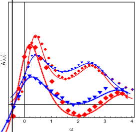
Figure 10: Experimenal data vs holographic theory: XAS data ; color red is for SrVO₃ and (color blue) is for CaVO₃. The data for SrVO₃ is from sekiyama2002genuine , and that for CaVO₃ is from inoue1995systematic . The parameters values we used $(m,p,k_{c},\mu)=(0.47,1.9,2.05,1.732)$ for red line and $(0.455,1.7,2.07,1.732)$ for blue line.

5 Discussion

In this paper we studied the phase diagram of a holographic model which can accommodate the physics of Mott transition. The key feature is the presence of gapped phase and the Free fermion point. The competition of the two generate pseudo-gap phase as an intermediate zone. Any line connecting the gapped and free fermion point in the phase space can be regarded as a an analogue of the Hubbard model. We report that all the phase change is smooth and we did not find any signal of instability in the spectral density within the unitarity bound $m<1/2$. Comparing the DMFT result on the Hubbard model with ours, three features agree with single site DMFT: the appearance of shoulder peak and transfer of the DOS to the shoulder peak and the maintenance of the central peak till the gap creation. However, due to the large asymmetry created by the chemical potential, three peak structure is not manifest since one of the shoulder is too weak. For the cluster DMFT and the hyperbolic embedding, there is an agreement in the appearance of the pseudo-gap. But again due to the asymmetry, the details are different.

What is the origin of the spectral asymmetry? If spatial dimension is bigger than 1, the momentum space light-cone $(\omega+\mu)^{2}-k^{2}=0$ is asymmetric because the region below the chemical potential is closer to the tip of the cone. In 1+1 dimensional theory we do not expect such asymmetry. The charge dependence of the interaction term enhanced this phenomena.

Apart from the asymmetry there is one more problem in this model. It turns out that for the model with dipole interaction, the filling fraction changes the interaction strength $p$, which is odd at first sight. This can be understood the if we note that $p$ always comes with $Q$, the charge density of RN black hole, so that increasing $p$ has the effect of increasing $Q$. Increasing $Q$ has the effect of increasing $\mu$ so that in the presence of the Fermi sea, the fermi level should look as if it is increased. In real material changing the coupling strength should not involve the effect of changing the particle number. Therefore we should conclude that the dipole term is not proper to model the Mott transition in a system where particle number is preserved.

We describe some future interests below. First, we need to find other gap creation mechanism which can realize the Mott transition such that spectral function maintains particle-hole symmetry at least approximately, lack of which is the most serious defect of present model in practical application. Second, we need to consider the back reaction of the background geometry. This is especially interesting due to the parallelism of holographic theory and the DMFT calculation near quantum critical pointPhysRevLett.107.026401 ; 2016arXiv160200131D . Third, when the gap is generated, the conformal invariance is also broken therefore the conformal unitarity condition that restricted us $m\leq 1/2$ is not much meaningful. Then, we should investigate beyond $m=1/2$. Next, we should study the fermions in the presence of the complex scalar, the superconducting order parameter. Also we did not investigated temperature and chemical potential evolutions much. It will gives most practical results to data fit. Many interesting questions are waiting analysis to accommodate the reality in the holographic model.

Appendix

Appendix A phase space of T=0

The phase diagram depends on temperature. We examined the phase space in zero temperature: Bad metal and its prime regions are reduced but not go away at $T=0$ because the presence of sharp peak itself does not guarantee that it is Fermi liquid. At $p=0$, the spectral function depends on the frequency $\sim\omega^{-2m}$ in alternative quantization we use. If $m$ is not large enough, localizing the spectral function to the Fermi surface can not be achieved so that it is far from Fermi liquid behavior. Therefore we need to distinguish the phase near the $m=0.5,p=0$, the free fermion point, from the phase near $m=0,p=0$, which is dubbed as bad metal region. Notice also that the zero temperature Fermi surface disappears very quickly (if not on m=1/2 line) as soon as we turn on T just a bit.

Bad-metal prime region shrinks to $m>0.45$ but it still exists. See figure 11 below.

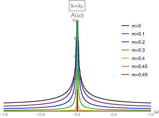
(a) $k=k_{F}$

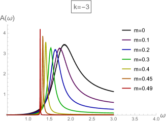
(b) $k=-3$

Figure 11: The spectral density at $T=0$ and $p=0$ at fixed momentum $k_{F}$. (a) Spectral density at $k=k_{F}$. There is sharp peak at $k_{F}$. As mass decreases, it is not localized at the fermi-surface and can not be classified as a Fermi liquid. (b) Spectral density at $k=-3$ also shows that it is broad for small mass. The hight decreases up to $m\sim 0.25$ and increases.

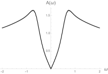
(a) $m=0$

(b) $m=0.45$

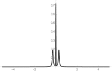
(c) $m=0.49$

Figure 12: Evolution of the spectral density at $T=0$ and $p=2$. BM’ region is much reduced at $T=0$ but still exist.

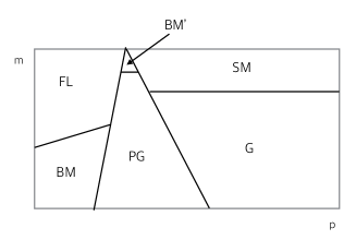
Figure 13: Schematic phase diagram at $T=0$.

Gapped phase and pseudo-gap phase expand such that much of the bad metal prime region become pseudo-gap at zero temperature. The phase boundary of gapped phase and pseudo-gap is moved to near p=3 at m=0 according to our criterion. The phase diagram is drawn schematically in the figure 13, where we do not find any qualitative change. However, the zero temperature phase diagram is not very useful to fit the data of the transition metal oxides. This is because typical data belong to bad metal prime phase, and at zero temperature, this relevant regime is tiny, therefore there is not much room to adjust the parameter to fit data. In this paper, we have drawn it at $T=0.1$, which gives a typical phase diagram and useful to us for data fitting.

Appendix B The role of $m$ and $p$

B.1 Gap generation versus Appearance of half-metal phase

Here we follow fixed mass line in the parameter space to see the evolution as we increase the $p$. We first study the lower half of the phase diagram by calculating its evolution along the line $m=0.1$ with increasing the dipole strength. The result is is drawn in Figures 14 (a)-(h), where three different phases appear:

1. Fig. 14 (a,e) $p=1$, bad metal phase with broadened peak with low height at Fermi level,

2. Fig. 14 (b,f) $p=2$, psuedo-gap phase with incomplete depletion of DOS at Fermi level.

3. Fig. 14 (c,g) $p=6$, gapped phase; Fig. 14 (d,h) $p=8$, gapped phase with increased gap size.

The overall feature of the evolution is from metalic to the insulating phase with pseudo gap phase in the middle and it agrees with our expectation.

(a) $p=1$

(b) $p=2$

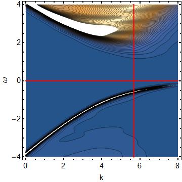
(c) $p=6$

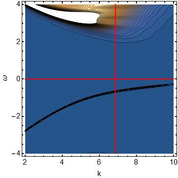
(d) $p=8$

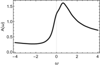
(e) $p=1$

(f) $p=2$

(g) $p=6$

(h) $p=8$

Figure 14: (a)-(d) on p-evolution of the DOS along the line m = 0.1 show appearance of and pseudo-gap and gapped phase; (e)-(h) spectral function along vertical red line in each figure (a)-(d). $k_{c}=1.65,2.46,5.68,6.86$ respectively from (e) to (h).

We now show the evolution along the line of $m=0.45$ with increasing $p$ to demonstrate the changes of phase in the upper half part of the phase diagram. The $\omega$-plots in Figures 15(e)-(h) are is along the red vertical redlines in Figure 15(a)-(d) respectively. We can see three different phases:

1. Gapless metalic phase with linear dispersion: it is a Fermi liquid (FL) regime.

2. The bad metal phase due to development of incomplete generation of conduction band.

3. New metalic phase which we call half-metal due to the development of the conduction band. half-metal because half of the DOS at the Fermi sea is depleted and moved to shoulder region.

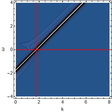
(a) $p=1$

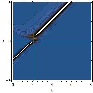
(b) $p=2$

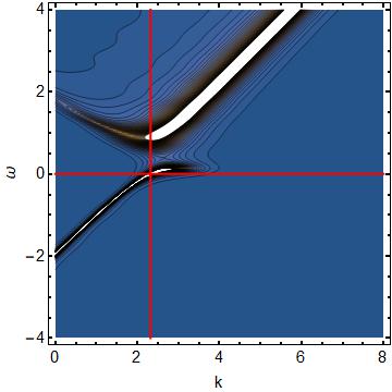
(c) $p=3$

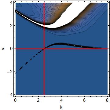
(d) $p=6$

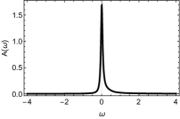
(e) $p=1$

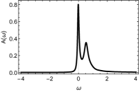
(f) $p=2$

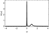
(g) $p=3$

(h) $p=6$

Figure 15: (a)-(d):$p$-evolution of the DOS at $m=0.45$ shows appearance of and bad metal prime and half-metal; (e)-(h) spectral function along vertical red line in each figure (a)-(d). We choose $k_{c}$ as $(1.74,2.08,2.32,2.48)$ respectively.

B.2 Bulk-mass evolution at fixed $p$

We now study the role of mass more systematically by calculating the evolution of the DOS at two nonzero fixed values of $p$, that is along two vertical lines $p=2.5$ and $p=6.0$ in phase dragram. In the Figure 16(a)-(h), the $m$-evolution along $p=0.2$ line is drawn, where a few physically interesting phases appear. From the figures 16(i)-(p), we can see that the bulk mass sharpens the peak at the Fermi surface consistently regardless of the value of $p$. One can see that increasing $m$ pushes up the new band so that gap is reduced. When the middle band crosses the Fermi level, central peak appears signaling the creation of the half-metalic phase. For both cases the final stage is hM phase.

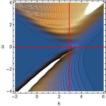
(a) $m=0$ $p=2.5$

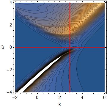
(b) $m=0.15$ $p=2.5$

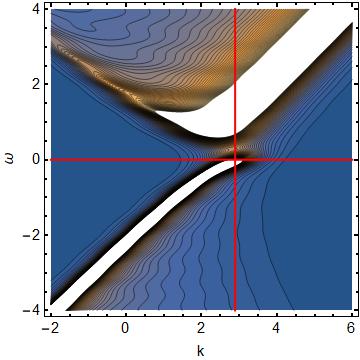
(c) $m=0.35$ $p=2.5$

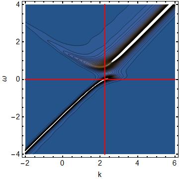
(d) $m=0.45$ $p=2.5$

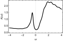
(e) $m=0$ $p=2.5$

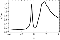
(f) $m=0.15$ $p=2.5$

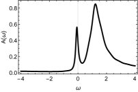
(g) $m=0.35$ $p=2.5$

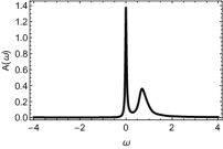
(h) $m=0.45$ $p=2.5$

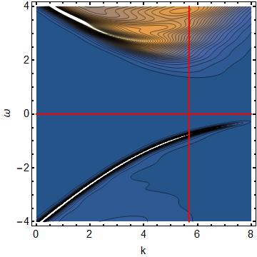
(i) $m=0$ $p=6$

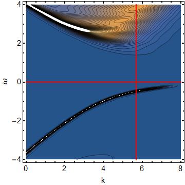
(j) $m=0.15$ $p=6$

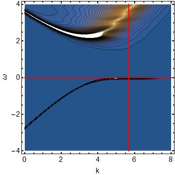
(k) $m=0.35$ $p=6$

(l) $m=0.45$ $p=6$

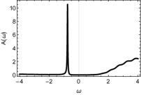
(m) $m=0$ $p=6$

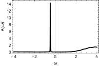
(n) $m=0.15$ $p=6$

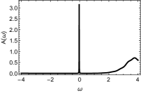
(o) $m=0.35$ $p=6$

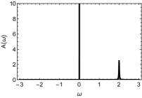
(p) $m=0.45$ $p=6$

Figure 16: (a)-(h): $m$- evolution of the spectral density with increasing $m$ with $p=2.5$. We choose $k_{c}$ as $(2.89,2.89,2.89,2.25)$ respectively. (i)-(p):Evolution of the spectral density at $p=6.0$. For both cases the final stage is hM phase. We choose $k_{c}$ as $(5.68,5.68,5.68,2.48)$ respectively.

Appendix C Symmetrized spectral function

Pseudo-gap data in the context of High-Tc superconductor theory is usually presented using symmetrized spectral function (SSF) norman1998phenomenology ; lee2007abrupt ; kondo2009competition . We present the result it in figure 17 for those who are already familiar to condensed matter literature.

(a) BM’ $(m=0.4,p=2)$

(b) PG $(m=0.1,p=2)$

Figure 17: Symmetrized spectral functions for Bad metal prime and psuedo-gap.

C.1 PES data with symmetrized spectral function

As we mentioned in the main text, the photoemission data can be fit by the holographic theory only when we symmetrize the spectral function in $\omega$: $A(\omega,k)\to f(A(\omega,k)+A(-\omega,k))$ fermion distribution function $f=1/(1+e^{E/kT})$. Although we do not have good reason to do it, the result is fantastic. In figure 18 we record the result for possible use in the future.

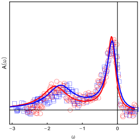
Figure 18: PES data with symmetrized spectral function: color red is for SrVO₃ and (color blue) is for CaVO₃. The data for SrVO₃ is from sekiyama2002genuine , and that for CaVO₃ is from inoue1995systematic . The parameters values we used are $(m,p,k_{c},\mu)=(0.47,2.2,2.08,1.732)$ for red line and $(0.47,2.05,2.04,1.732)$ for blue line.

C.2 Evolution along two embeddings

Here we give four embeddings corresponding to the four colored lines in Figure 19 and corresponding spectral functions using the symmetrized embedding which was used in the early stage of the work.

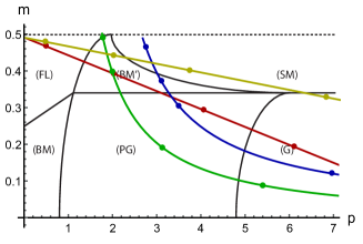
Figure 19: An embedding defines a path from gapless to gapped phase in holographic model: $\alpha=1/40$ (1/20) for yellow (red) line in linear embedding. $\beta=$8/9 (4/3) for blue (green) curve in hyperbolic embedding.

(a)

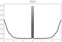
(b)

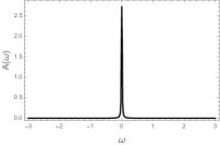
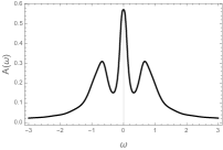
(c)

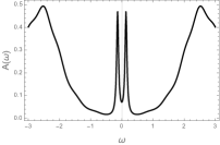
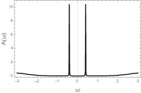
(d)

Figure 20: $U$-evolutions for linear Embedding. (a)-(d) are at marked point of embedding diagram for upper (Yellow) line, (e)-(h) for for lower (Red) line.

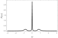
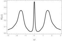
(a)

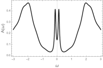
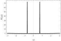
(b)

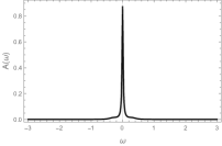
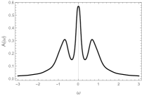
(c)

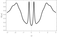
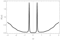
(d)

Figure 21: $U$-evolutions for Hyperbolic Embedding ($V\neq 0$). (a)-(d) for upper (Blue) curve, (e)-(h) for lower (Green) curve, Spectral functions at $k_{c}$ for $V\neq 0$ (Green Curve).

- (1) N. F. MOTT, Metal-insulator transition, Reviews of Modern Physics 40 (1968) 677–683.
- (2) J. Zaanen, Y.-W. Sun, Y. Liu and K. Schalm, Holographic Duality in Condensed Matter Physics. Cambridge Univ. Press, 2015.
- (3) S. A. Hartnoll, A. Lucas and S. Sachdev, Holographic quantum matter, 1612.07324.
- (4) S.-S. Lee, A Non-Fermi Liquid from a Charged Black Hole: A Critical Fermi Ball, Phys. Rev. D79 (2009) 086006, [0809.3402].
- (5) H. Liu, J. McGreevy and D. Vegh, Non-Fermi liquids from holography, Phys. Rev. D83 (2011) 065029, [0903.2477].
- (6) T. Faulkner, H. Liu, J. McGreevy and D. Vegh, Emergent quantum criticality, Fermi surfaces, and AdS(2), Phys. Rev. D83 (2011) 125002, [0907.2694].
- (7) T. Faulkner, N. Iqbal, H. Liu, J. McGreevy and D. Vegh, Holographic non-Fermi liquid fixed points, Phil. Trans. Roy. Soc. A 369 (2011) 1640, [1101.0597].
- (8) T. Faulkner, N. Iqbal, H. Liu, J. McGreevy and D. Vegh, Charge transport by holographic Fermi surfaces, Phys. Rev. D88 (2013) 045016, [1306.6396].
- (9) M. Edalati, R. G. Leigh, K. W. Lo and P. W. Phillips, Dynamical Gap and Cuprate-like Physics from Holography, Phys. Rev. D83 (2011) 046012, [1012.3751].
- (10) M. Edalati, R. G. Leigh and P. W. Phillips, Dynamically Generated Mott Gap from Holography, Phys. Rev. Lett. 106 (2011) 091602, [1010.3238].
- (11) G. Vanacore and P. W. Phillips, Minding the Gap in Holographic Models of Interacting Fermions, Phys. Rev. D90 (2014) 044022, [1405.1041].
- (12) G. Vanacore, S. T. Ramamurthy and P. W. Phillips, Evolution of Holographic Fermi Arcs from a Mott Insulator, 1508.02390.
- (13) Y. Ling, P. Liu, C. Niu, J.-P. Wu and Z.-Y. Xian, Holographic fermionic system with dipole coupling on Q-lattice, JHEP 12 (2014) 149, [1410.7323].
- (14) M. Cubrovic, J. Zaanen and K. Schalm, String Theory, Quantum Phase Transitions and the Emergent Fermi-Liquid, Science 325 (2009) 439–444, [0904.1993].
- (15) M. Cubrovic, J. Zaanen and K. Schalm, Constructing the AdS Dual of a Fermi Liquid: AdS Black Holes with Dirac Hair, JHEP 10 (2011) 017, [1012.5681].
- (16) M. V. Medvedyeva, E. Gubankova, M. Čubrović, K. Schalm and J. Zaanen, Quantum corrected phase diagram of holographic fermions, JHEP 12 (2013) 025, [1302.5149].
- (17) A. Donos and S. A. Hartnoll, Interaction-driven localization in holography, Nature Phys. 9 (2013) 649–655, [1212.2998].
- (18) T. Andrade, A. Krikun, K. Schalm and J. Zaanen, Doping the holographic Mott insulator, 1710.05791.
- (19) M. Fujita, S. Harrison, A. Karch, R. Meyer and N. M. Paquette, Towards a Holographic Bose-Hubbard Model, JHEP 04 (2015) 068, [1411.7899].
- (20) M. Ammon, J. Erdmenger, M. Kaminski and A. O’Bannon, Fermionic Operator Mixing in Holographic p-wave Superfluids, JHEP 05 (2010) 053, [1003.1134].
- (21) Y. Seo, G. Song, P. Kim, S. Sachdev and S.-J. Sin, Holography of the Dirac Fluid in Graphene with two currents, Phys. Rev. Lett. 118 (2017) 036601, [1609.03582].
- (22) Y. Seo, G. Song and S.-J. Sin, Strong Correlation Effects on Surfaces of Topological Insulators via Holography, Phys. Rev. B96 (2017) 041104, [1703.07361].
- (23) Y. Seo, G. Song, C. Park and S.-J. Sin, Small Fermi Surfaces and Strong Correlation Effects in Dirac Materials with Holography, JHEP 10 (2017) 204, [1708.02257].
- (24) U. Gursoy, E. Plauschinn, H. Stoof and S. Vandoren, Holography and ARPES Sum-Rules, JHEP 05 (2012) 018, [1112.5074].
- (25) A. Georges, G. Kotliar, W. Krauth and M. J. Rozenberg, Dynamical mean-field theory of strongly correlated fermion systems and the limit of infinite dimensions, Rev. Mod. Phys. 68 (Jan, 1996) 13–125.
- (26) Y. Zhang and M. Imada, Pseudogap and mott transition studied by cellular dynamical mean-field theory, Physical Review B 76 (2007) 045108.
- (27) A. Sekiyama, H. Fujiwara, S. Imada, H. Eisaki, S. Uchida, K. Takegahara et al., Genuine electronic states of vanadium perovskites revealed by high-energy photoemission, arXiv preprint cond-mat/0206471 (2002) .
- (28) I. Inoue, I. Hase, Y. Aiura, A. Fujimori, Y. Haruyama, T. Maruyama et al., Systematic development of the spectral function in the 3 d 1 mott-hubbard system ca 1- x sr x vo 3, Physical review letters 74 (1995) 2539.
- (29) M. Norman, M. Randeria, H. Ding and J. Campuzano, Phenomenology of the low-energy spectral function in high-t c superconductors, Physical Review B 57 (1998) R11093.
- (30) W. Lee, I. Vishik, K. Tanaka, D. Lu, T. Sasagawa, N. Nagaosa et al., Abrupt onset of a second energy gap at the superconducting transition of underdoped bi2212, Nature 450 (2007) 81.
- (31) T. Kondo, R. Khasanov, T. Takeuchi, J. Schmalian and A. Kaminski, Competition between the pseudogap and superconductivity in the high-t c copper oxides, Nature 457 (2009) 296.
- (32) E. Pavarini, E. Koch, D. Vollhardt and A. Lichtenstein, DMFT at 25: Infinite Dimensions: Lecture Notes of the Autumn School on Correlated Electrons 2014, vol. 4. Forschungszentrum Jülich, 2014.
- (33) A. Sekiyama, H. Fujiwara, S. Imada, S. Suga, H. Eisaki, S. Uchida et al., Mutual experimental and theoretical validation of bulk photoemission spectra of , Physical review letters 93 (2004) 156402.
- (34) I. Nekrasov, G. Keller, D. Kondakov, A. Kozhevnikov, T. Pruschke, K. Held et al., Comparative study of correlation effects in cavo3 and srvo3, Physical review B. Condensed matter and materials physics 72 (2005) 155106–1.
- (35) H. Park, K. Haule and G. Kotliar, Cluster dynamical mean field theory of the mott transition, Phys. Rev. Lett. 101 (Oct, 2008) 186403.
- (36) H. Terletska, J. Vučičević, D. Tanasković and V. Dobrosavljević, Quantum critical transport near the mott transition, Phys. Rev. Lett. 107 (Jul, 2011) 026401.
- (37) V. Dobrosavljevic and D. Tanaskovic, Wigner-Mott quantum criticality: from 2D-MIT to 3He and Mott organics, ArXiv e-prints (Jan., 2016) , [1602.00131].