Banded Spatio-Temporal Autoregressions

Abstract

We propose a new class of spatio-temporal models with unknown and banded autoregressive coefficient matrices. The setting represents a sparse structure for high-dimensional spatial panel dynamic models when panel members represent economic (or other type) individuals at many different locations. The structure is practically meaningful when the order of panel members is arranged appropriately. Note that the implied autocovariance matrices are unlikely to be banded, and therefore, the proposal is radically different from the existing literature on the inference for high-dimensional banded covariance matrices. Due to the innate endogeneity, we apply the least squares method based on a Yule-Walker equation to estimate autoregressive coefficient matrices. The estimators based on multiple Yule-Walker equations are also studied. A ratio-based method for determining the bandwidth of autoregressive matrices is also proposed. Some asymptotic properties of the inference methods are established. The proposed methodology is further illustrated using both simulated and real data sets.

Keywords: Banded coefficient matrices, Least squares estimation, Spatial panel dynamic models, Yule-Walker equation.

1 Introduction

One common feature in most literature on spatial econometrics is to specify each autoregressive coefficient matrix in a spatial autoregressive or a spatial dynamic panel model as a product of an unknown scalar parameter and a known spatial weight matrix, and the focus of the inference is on those a few unknown scalar parameters placed in front of spatial weight matrices. See, for example, Cliff and Ord (1973), Yu et al. (2008), Lee and Yu (2010), Lin and Lee (2010), Kelejian and Prucha (2010), Su (2012), and Yu et al. (2012). Using spatial weight matrices reflects the initial thinking that spatial dependence measures should take into account both spatial locations and feature variables at locations simultaneously. A weight matrix may reflect the closeness of different spatial locations. It needs to be specified subjectively. There are multiple weighting possibilities including inverse distance, fixed distance, space-time window, $K$-nearest neighbors, contiguity, and spatial interaction. The conceptualization specified in spatial matrices for a particular analysis imposes a specific structure onto the data collected across the locations. Ideally one would select a conceptualization that best reflects how the features actually interact with each other in the real world.

For a given application it is not always obvious how to specify a pertinent spatial weight matrix. Consequently the resulting spatial autoregressive model may be incapable to accommodate adequately the dependent structure across different locations. Dou et al. (2016) considers the models which employ different scalar coefficients, in front of spatial weight matrices, for different locations. By drawing energy and inspiration from the recent development in sparse high-dimensional (auto)regressions (Guo et al. 2016), we propose in this paper a new class of spatio-temporal models in which autoregressive coefficient matrices are completely unknown but are assumed to be banded, i.e. the non-zero coefficients only occur within the narrow band around the main diagonals. This avoids the difficulties in specifying spatial weight matrices subjectively. The setting specifies autoregressions over neighbouring locations only. The underpinning idea rests on the fact that in many applications it is enough to collect information from neighbouring locations, and then the information from farther locations become redundant. Of course the banded structure relies on arranging all the locations concerned in a unilateral order. In practice, an appropriate ordering can be deduced from subject knowledge aided by statistical tools such as cross-validation; see Section 4.2. It is worth pointing out that the implied autocovariance matrices are unlikely to be banded in spite of the banded autoregressive coefficient matrices.

Guo et al. (2016) considered banded autoregressive models for vector time series, and estimated the coefficient matrices by a componentwise least squares method. Unfortunately their method does not apply to our setting, due to the endogeneity in spatial autoregressive models. Instead we adapt a version of generalized method of moments estimation based on a Yule-Walker equation (Dou et al. 2016). Furthermore the estimation of the parameters based on multiple Yule-Walker equations is also investigated. The asymptotic property of the estimation is established when the dimensionality $p$ (i.e. the number of panels) diverges together with the sample size $n$ (i.e. the length of the observed time series). The convergence rates of the estimators are the same with those in Dou et al. (2016). More precisely, the estimated coefficients are asymptotically normal when $p=o(\sqrt{n})$, and is consistent when $p=o(n)$.

In practice, the width of the nonzero coefficient bands in the coefficient matrices needs to be estimated. We propose a ratio-based estimation method which is shown to lead to a consistent estimated width when both $n$ and $p$ tend to infinity.

The rest of the paper is organized as follows. We specify the class of models and the associate estimation methods in Section 2. The asymptotic properties are presented in Section 3. The numerical illustration with both simulated and real data sets are reported in Section 4. All technical proofs are relegated into an Appendix.

2 Model and estimation method

2.1 Spatio-temporal regression model

Consider the spatio-temporal regression

$$\mathbf{y}_{t}={\mathbf{A}}\mathbf{y}_{t}+{\mathbf{B}}\mathbf{y}_{t-1}+\mbox{\boldmath$\varepsilon$}_{t},$$ (2.1)

where $\mathbf{y}_{t}=(y_{1,t},...,y_{p,t})^{\top}$ represents the observations collected from $p$ locations at time $t$, $\mbox{\boldmath$\varepsilon$}_{t}=({{\varepsilon}}_{1,t},{{\varepsilon}}_{2,t},...,{{\varepsilon}}_{p,t})^{\top}$ is the innovation at time $t$ and satisfies the condition that

$$E(\mbox{\boldmath$\varepsilon$}_{t})=0,\qquad\textnormal{Var}(\mbox{\boldmath$\varepsilon$}_{t})=\boldsymbol{\Sigma}_{\varepsilon}\quad\text{and}\qquad\mbox{cov}(\mathbf{y}_{t-j},\mbox{\boldmath$\varepsilon$}_{t})=0\;\;{\rm for\;all}\;j\geq 1,$$

where $\boldsymbol{\Sigma}_{\varepsilon}$ is an unknown positive definite matrix. Furthermore we assume that ${\mathbf{A}}\equiv(a_{i,j})$ and ${\mathbf{B}}\equiv(b_{i,j})$ are $p\times p$ unknown banded coefficient matrices, i.e.,

$$a_{i,j}=b_{i,j}=0\ \ \textnormal{for all}\ \ |i-j|>k_{0},$$ (2.2)

and $a_{i,i}=0$ for $1\leq i\leq p$. We call $k_{0}$ ($<p$) the bandwidth parameter which is an unknown positive integer. In the above model (2.1), ${\mathbf{A}}$ captures the pure spatial dependency among different locations, and ${\mathbf{B}}$ captures the dynamic dependency.

Model (2.1) extends the popular spatial dynamic panel data models (SDPD) substantially. The standard SDPD assumes that each coefficient matrix is a product of a known linkage matrix and an unknown scalar parameter, see, e.g., Yu et al. (2008) and Yu et al. (2012). While some sparse structure has to be imposed in order to conduct meaningful inference when $p$ is large, the inflexibility of having merely single parameter in each regression coefficient matrix is too restrictive, see, e.g., Dou et al. (2016). Note that the condition $a_{i,j}=b_{i,j}=0$ does not imply Cov$(y_{i,t},y_{j,t})=0$ or Cov$(y_{i,t},y_{j,t-1})=0$, regardless of the covariance structure of $\mbox{\boldmath$\varepsilon$}_{t}$, see (2.4) below. Instead the banded sparse structure imposed in (2.1) implies that conditionally on the information among the ‘closest neighbours’, the information from farther locations become redundant. This reflects the common sense in many practical situations, though the definition of the closeness is case-dependent.

Let ${\mathbf{I}}_{p}-{\mathbf{A}}$ be invertible, and all the eigenvalues of $({\mathbf{I}}_{p}-{\mathbf{A}})^{-1}{\mathbf{B}}$ be smaller than $1$ in modulus, where ${\mathbf{I}}_{p}$ denotes the $p\times p$ identity matrix. Then model (2.1) can be rewritten as

$$\mathbf{y}_{t}=({\mathbf{I}}_{p}-{\mathbf{A}})^{-1}{\mathbf{B}}\mathbf{y}_{t-1}+({\mathbf{I}}_{p}-{\mathbf{A}})^{-1}\mbox{\boldmath$\varepsilon$}_{t},$$ (2.3)

which admits a (weakly) stationary solution of $\mathbf{y}_{t}$. For this stationary process, $E{\mathbf{y}}_{t}=0$, and the Yule-Walker equations are

$$\boldsymbol{\Sigma}_{0}=({\mathbf{I}}_{p}-{\mathbf{A}})^{-1}{\mathbf{B}}\boldsymbol{\Sigma}_{1}^{\top}+({\mathbf{I}}_{p}-{\mathbf{A}})^{-1}\boldsymbol{\Sigma}_{\varepsilon}({\mathbf{I}}_{p}-{\mathbf{A}}^{\top})^{-1},\quad\boldsymbol{\Sigma}_{j}=({\mathbf{I}}_{p}-{\mathbf{A}})^{-1}{\mathbf{B}}\boldsymbol{\Sigma}_{j-1}\;\;{\rm for}\;\;j\geq 1,$$ (2.4)

where $\boldsymbol{\Sigma}_{j}=\mbox{cov}(\mathbf{y}_{t+j},\mathbf{y}_{t})$ for any $j\geq 0$. Since the inverse of a banded matrix is unlikely to be banded, $\boldsymbol{\Sigma}_{0}$, therefore also $\boldsymbol{\Sigma}_{j}$ are not banded in general. We refer to §4.3 of Golub and van Loan (2013), and Kılıç and Stanica (2013) for the properties and the computation of banded matrices and their inverses.

Throughout this paper, $\mathbf{y}_{t}$ is referred to as a stationary process defined by (2.3).

2.2 Generalized Yule-Walker estimation

As $\mathbf{y}_{t}$ appears on both sides of equation (2.1) and $\mathbf{y}_{t}$ is correlated with $\mbox{\boldmath$\varepsilon$}_{t}$, the least squares estimation based on regressing $\mathbf{y}_{t}$ on $(\mathbf{y}_{t},\mathbf{y}_{t-1})$ directly leads to inconsistent estimators, due to the innate endogeneity of (2.1). We observe that the second equation of (2.4) implies

$$\boldsymbol{\Sigma}_{1}^{\top}{\mathbf{e}}_{i}=\boldsymbol{\Sigma}_{1}^{\top}{\mathbf{a}}_{i}+\boldsymbol{\Sigma}_{0}{\mathbf{b}}_{i}\equiv{\mathbf{V}}_{i}\boldsymbol{\beta}_{i},\quad i=1,...,p,$$ (2.5)

where ${\mathbf{e}}_{i}$ denotes the $p\times 1$ unit vector with 1 as its $i$-th element, ${\mathbf{A}}^{\top}=({\mathbf{a}}_{1},\cdots,{\mathbf{a}}_{p})$, ${\mathbf{B}}^{\top}=({\mathbf{b}}_{1},\cdots,{\mathbf{b}}_{p})$, $\boldsymbol{\beta}_{i}$ is the $\tau_{i}\times 1$ vector obtained by stacking together the non-zero elements in ${\mathbf{a}}_{i}$ and ${\mathbf{b}}_{i}$, and ${\mathbf{V}}_{i}$ is the $p\times\tau_{i}$ matrix consisting of the corresponding columns of $\boldsymbol{\Sigma}_{1}^{\top}$ and $\boldsymbol{\Sigma}_{0}$. It follows from (2.2) that

$$\tau_{i}\equiv\tau_{i}(k_{0})=\left\{\begin{array}[]{ll}2(k_{0}+i)-1&1\leq i\leq k_{0},\\ 4k_{0}+1&k_{0}<i\leq p-k_{0},\\ 2(k_{0}+p-i)+1&p-k_{0}<i\leq p.\end{array}\right.$$ (2.6)

We first treat the bandwidth $k_{0}$ as a known parameter and apply a version of generalized method of moment estimation based on (2.5), i.e. we apply least squares method to estimate $({\mathbf{A}},{\mathbf{B}})$ by solving the following minimization problems

$$\mathop{\min}_{{\mathbf{a}}_{i},{\mathbf{b}}_{i}}\|\widehat{\boldsymbol{\Sigma}}_{1}^{\top}{\mathbf{e}}_{i}-\widehat{\boldsymbol{\Sigma}}_{1}^{\top}{\mathbf{a}}_{i}-\widehat{\boldsymbol{\Sigma}}_{0}{\mathbf{b}}_{i}\|_{2}^{2},\quad i=1,...,p,$$ (2.7)

where

$$\widehat{\boldsymbol{\Sigma}}_{1}=\frac{1}{n}\sum_{t=2}^{n}\mathbf{y}_{t}\mathbf{y}_{t-1}^{\top}\ \quad\text{and}\quad\ \ \widehat{\boldsymbol{\Sigma}}_{0}=\frac{1}{n}\sum_{t=2}^{n}\mathbf{y}_{t-1}\mathbf{y}_{t-1}^{\top}.$$ (2.8)

We omit the term $\mathbf{y}_{n}\mathbf{y}_{n}^{T}$ in the definition of $\widehat{\boldsymbol{\Sigma}}_{0}$ above for a minor technical convenience which ensures the validity of (2.11) and (2.12) below. Let $\widehat{{\mathbf{z}}}_{i}=\widehat{\boldsymbol{\Sigma}}_{1}^{\top}{\mathbf{e}}_{i}$ and $\widehat{\mathbf{V}}_{i}$ be the sample version of ${\mathbf{V}}_{i}$ in (2.5), (2.7) leads to the least square estimator

$$\widehat{\boldsymbol{\beta}}_{i}=(\widehat{\mathbf{V}}_{i}^{\top}\widehat{\mathbf{V}}_{i})^{-1}\widehat{\mathbf{V}}_{i}^{\top}\widehat{\mathbf{z}}_{i},\quad i=1,...,p.$$ (2.9)

The corresponding residual sum of squares is

$$\mbox{RSS}_{i}\equiv\mbox{RSS}_{i}(k_{0})={1\over p}\|\widehat{\mathbf{z}}_{i}-\widehat{\mathbf{V}}_{i}\widehat{\boldsymbol{\beta}}_{i}\|^{2},\quad i=1,...,p.$$ (2.10)

We note that (2.10) is a function of $k_{0}$, while in practice, $k_{0}$ is unknown and we will propose a consistent way to estimate $k_{0}$ in Section 2.4 below.

Combining all the estimators in (2.9) together leads to the estimators for ${\mathbf{A}}$ and ${\mathbf{B}}$, which are denoted by, respectively, $\widehat{\mathbf{A}}$ and $\widehat{\mathbf{B}}$.

It follows from (2.1), (2.2) and (2.8) that

$$\widehat{\mathbf{z}}_{i}={1\over n}\sum_{t=2}^{n}{\mathbf{y}}_{t-1}y_{i,t}={1\over n}\sum_{t=2}^{n}{\mathbf{y}}_{t-1}({\mathbf{y}}_{t}^{\top}{\mathbf{a}}_{i}+{\mathbf{y}}_{t-1}^{\top}{\mathbf{b}}_{i}+{{\varepsilon}}_{i,t})=\widehat{\mathbf{V}}_{i}\boldsymbol{\beta}_{i}+{1\over n}\sum_{t=2}^{n}{\mathbf{y}}_{t-1}{{\varepsilon}}_{i,t}.$$ (2.11)

Hence it holds that

$$\widehat{\boldsymbol{\beta}}_{i}-\boldsymbol{\beta}_{i}={1\over n}(\widehat{\mathbf{V}}_{i}^{\top}\widehat{\mathbf{V}}_{i})^{-1}\widehat{\mathbf{V}}_{i}^{\top}\sum_{t=2}^{n}{\mathbf{y}}_{t-1}{{\varepsilon}}_{i,t},\quad i=1,...,p.$$ (2.12)

In the above expressions,

$$\widehat{\mathbf{V}}_{i}={1\over n}\sum_{t=2}^{n}{\mathbf{y}}_{t-1}{\mathbf{u}}_{t,i}^{\top},$$ (2.13)

where ${\mathbf{u}}_{t,i}$ is a $\tau_{i}\times 1$ vectors consisting of $y_{j,t}$ for $j\in S_{i}$ and $y_{\ell,t-1}$ for $\ell\in S_{i}^{+}$, where

$$S_{i}=\{j:1\leq j\leq p,\ 1\leq|j-i|\leq k_{0}\}\quad\text{and}\quad S^{+}_{i}=\{j:1\leq j\leq p,\ |j-i|\leq k_{0}\}.$$

2.3 A root-$n$ consistent estimator for large $p$

By Theorem 2 in Section 3 below, the estimator (2.9) admits a convergence rate different from $\sqrt{n}$ when $p/\sqrt{n}\rightarrow\infty$. This is an over-determined case in the sense that the number of estimation equations is far greater than the number of parameters to be estimated. Similar results can also be found in Dou et al. (2016) and Chang et al. (2015), among others. Borrowing the idea from Dou et al. (2016), we propose an alternative estimator, which reduces the number of the estimation equations from $p$ to a smaller constant. The resulting estimator restores the $\sqrt{n}$-consistency and is also asymptotically normal.

Note that, the $\ell$-th row of $\widehat{\mathbf{V}}_{i}$ is ${\mathbf{e}}_{\ell}^{\top}\widehat{\mathbf{V}}_{i}$. By (2.13), this can be further expressed as ${1\over n}{\mathbf{e}}_{\ell}^{\top}\sum_{t=2}^{n}{\mathbf{y}}_{t-1}{\mathbf{u}}_{t,i}^{\top},$ which is the sample covariance between $y_{l,t-1}$ and ${\mathbf{u}}_{t,i}.$ Then, the strength of the correlation between $y_{\ell,t-1}$ and ${\mathbf{u}}_{t,i}$ can be measured by

$$\delta_{\ell}^{(i)}={1\over n}\sum_{t=2}^{n}\Big{(}\sum_{j\in S_{i}}|y_{\ell,t-1}y_{j,t}|+\sum_{j\in S^{+}_{i}}|y_{\ell,t-1}y_{j,t-1}|\Big{)}.$$ (2.14)

When $\delta_{\ell}^{(i)}$ is close to 0, the $\ell$-th equation in (2.5) carries little information on $\boldsymbol{\beta}_{i}$. Since our concern is the estimation for $\boldsymbol{\beta}_{i}$, we may only keep the $\ell$-th equation in (2.5) and hence (2.7) with the $d_{i}$ largest $\delta_{\ell}^{(i)}$.

Let ${\mathbf{w}}_{t-1}^{i}\in d_{i}\times 1$ be the sub-vector of ${\mathbf{y}}_{t-1}$. Specifically, ${\mathbf{w}}_{t-1}^{i}$ consists of those $y_{\ell,t-1}$ with the $d_{i}$ largest $\delta_{\ell}^{(i)}$. Then, we can obtain the new estimator as

$$\widetilde{\boldsymbol{\beta}}_{i}=(\widetilde{\mathbf{W}}_{i}^{\top}\widetilde{\mathbf{W}}_{i})^{-1}\widetilde{\mathbf{W}}_{i}^{\top}\widetilde{\mathbf{z}}_{i},\quad i=1,...,p,$$ (2.15)

where

$$\widetilde{\mathbf{W}}_{i}={1\over n}\sum_{t=2}^{n}{\mathbf{w}}_{t-1}^{i}{\mathbf{u}}_{t,i}^{\top}\quad\mbox{and}\quad\widetilde{\mathbf{z}}_{i}={1\over n}\sum_{t=2}^{n}{\mathbf{w}}_{t-1}^{i}y_{i,t}.$$ (2.16)

Therefore,

$$\widetilde{\boldsymbol{\beta}}_{i}-\boldsymbol{\beta}_{i}={1\over n}(\widetilde{\mathbf{W}}_{i}^{\top}\widetilde{\mathbf{W}}_{i})^{-1}\widetilde{\mathbf{W}}_{i}^{\top}\sum_{t=2}^{n}{\mathbf{w}}_{t-1}^{i}{{\varepsilon}}_{i,t},\quad i=1,...,p.$$

Theorem 3 in Section 3 shows the asymptotic normality of the above estimator provided that the number of estimation equations used satisfies condition $d_{i}=o_{p}(\sqrt{n})$. In practice, $d_{i}$ should be a prescribed number and Theorem 3 is valid as long as the condition $d_{i}=o_{p}(\sqrt{n})$ holds uniformly for all $i$.

2.4 Determination of bandwidth parameter $k_{0}$

In practice, the bandwidth parameter $k_{0}$ is unknown. We propose below a method to estimate it. Similar ideas can be found in Lam et al. (2011) and Lam and Yao (2012) for determining the number of factors in time series factor modelling.

Let $K\geq 1$ be a known upper bound of $k_{0}$. Our estimation method is based on the following simple observation: If we replace $(\widehat{\boldsymbol{\Sigma}}_{0},\widehat{\boldsymbol{\Sigma}}_{1})$ in (2.7) by the true $(\boldsymbol{\Sigma}_{0},\boldsymbol{\Sigma}_{1})$, the corresponding true value of $\mbox{RSS}_{i}(k)$ is positive and finite for $1\leq k<k_{0}$, and is equal to 0 for $k_{0}\leq k\leq K$. Thus the ratio $\mbox{RSS}_{i}(k-1)\big{/}\mbox{RSS}_{i}(k)$ is finite for $k<k_{0}$, $\mbox{RSS}_{i}(k_{0}-1)\big{/}\mbox{RSS}_{i}(k_{0})$ is excessively large, and $\mbox{RSS}_{i}(k-1)\big{/}\mbox{RSS}_{i}(k)$ is effectively ‘0/0’ for $k>k_{0}$.

To avoid the singularities when $k>k_{0}$, we introduce a small factor $w_{n}={C}/{n}$ in the ratio for some constant $C>0$. A ratio-based estimator for $k_{0}$ is defined as

$$\widehat{k}=\max_{1\leq i\leq p}\arg\max_{1<k\leq K}\frac{\mbox{RSS}_{i}(k-1)+w_{n}}{\mbox{RSS}_{i}(k)+w_{n}},$$ (2.17)

where $K\geq 1$ is a prescribed integer. Our numerical study shows that the procedure is insensitive to the choice of $K$ provided that $K\geq k_{0}$. In practice, we often choose $K$ to be $[n^{1/2}]$ or choose $K$ by checking the curvature of the ratio in (2.17) directly.

2.5 Estimation with multiple Yule-Walker equations

In Section 2.3, we have established a $\sqrt{n}$-consistent estimator for $\boldsymbol{\beta}_{i}$ with fewer estimation equations. However, this does not necessarily improve the estimation accuracy since we only make use of partial information for the parameters. In Dou et al. (2016), the estimation of the parameters is based on only one Yule-Walker equation. In view of the equations in (2.4), we may also estimate $({\mathbf{A}},{\mathbf{B}})$ using more than one Yule-Walker equations, and therefore we have more information for ${\mathbf{A}}$ and ${\mathbf{B}}$. Let $r$ be a prescribed positive integer, we consider the following $r$ Yule-Walker equations:

$$\left(\begin{array}[]{c}\boldsymbol{\Sigma}_{1}^{\top}\\ \boldsymbol{\Sigma}_{2}^{\top}\\ \vdots\\ \boldsymbol{\Sigma}_{r}^{\top}\end{array}\right)=\left(\begin{array}[]{c}\boldsymbol{\Sigma}_{1}^{\top}\\ \boldsymbol{\Sigma}_{2}^{\top}\\ \vdots\\ \boldsymbol{\Sigma}_{r}^{\top}\end{array}\right){\mathbf{A}}^{\top}+\left(\begin{array}[]{c}\boldsymbol{\Sigma}_{0}^{\top}\\ \boldsymbol{\Sigma}_{1}^{\top}\\ \vdots\\ \boldsymbol{\Sigma}_{r-1}^{\top}\end{array}\right){\mathbf{B}}^{\top}.$$ (2.18)

Denote

$$\widehat{\mathbf{x}}_{i}=\left(\begin{array}[]{c}\widehat{\boldsymbol{\Sigma}}_{1}^{\top}\\ \widehat{\boldsymbol{\Sigma}}_{2}^{\top}\\ \vdots\\ \widehat{\boldsymbol{\Sigma}}_{r}^{\top}\end{array}\right){\mathbf{e}}_{i}\quad\text{and}\quad\widehat{\mathbf{G}}=\left(\begin{array}[]{cc}\widehat{\boldsymbol{\Sigma}}_{1}^{\top}&\widehat{\boldsymbol{\Sigma}}_{0}\\ \widehat{\boldsymbol{\Sigma}}_{2}^{\top}&\widehat{\boldsymbol{\Sigma}}_{1}^{\top}-\frac{1}{n}{\mathbf{y}}_{n-1}{\mathbf{y}}_{n}^{\top}\\ \vdots&\vdots\\ \widehat{\boldsymbol{\Sigma}}_{r}^{\top}&\widehat{\boldsymbol{\Sigma}}_{r-1}^{\top}-\frac{1}{n}{\mathbf{y}}_{n-r+1}{\mathbf{y}}_{n}^{\top}\end{array}\right),$$ (2.19)

where $\widehat{\boldsymbol{\Sigma}}_{j}=\frac{1}{n}\sum_{t=j+1}^{n}{\mathbf{y}}_{t}{\mathbf{y}}_{t-j}^{\top}$ for $j\geq 1$. For technical convenience, we remove the last term of $\widehat{\boldsymbol{\Sigma}}_{j}^{\top}$ in the second half columns of $\widehat{\mathbf{G}}$ for $j\geq 1$.

By a similar argument as that in Section 2.2, we apply least squares method to estimate $({\mathbf{A}},{\mathbf{B}})$ by solving the following minimization problems

$$\mathop{\min}_{\boldsymbol{\theta}_{i}}\|\widehat{\mathbf{x}}_{i}-\widehat{\mathbf{G}}_{i}\boldsymbol{\theta}_{i}\|_{2}^{2},\quad i=1,...,p,$$ (2.20)

where $\boldsymbol{\theta}_{i}$ is a $\tau_{i}\times 1$ vector and $\widehat{\mathbf{G}}_{i}$ is the $rp\times\tau_{i}$ submatrix of $\widehat{\mathbf{G}}$ corresponding to the nonzero elements of ${\mathbf{a}}_{i}$ and ${\mathbf{b}}_{i}$. For each $i$, we denote $\widehat{\widehat{\boldsymbol{\beta}}}_{i}$ the solution to the $i$-th equation of (2.20). Then it follows from (2.20) that

$$\widehat{\widehat{\boldsymbol{\beta}}}_{i}=(\widehat{\mathbf{G}}_{i}^{\top}\widehat{\mathbf{G}}_{i})^{-1}\widehat{\mathbf{G}}_{i}^{\top}\widehat{\mathbf{x}}_{i},\quad i=1,...,p.$$ (2.21)

Combining all the estimators in (2.9) together leads to the estimators for ${\mathbf{A}}$ and ${\mathbf{B}}$ which are denoted by, respectively, $\widehat{\widehat{\mathbf{A}}}$ and $\widehat{\widehat{\mathbf{B}}}$.

Let $\mathbf{f}_{{{\varepsilon}}_{i}}=(\frac{1}{n}\sum_{t=2}^{n}{\mathbf{y}}_{t-1}^{\top}{{\varepsilon}}_{i,t},\frac{1}{n}\sum_{t=3}^{n}{\mathbf{y}}_{t-2}^{\top}{{\varepsilon}}_{i,t},...,\frac{1}{n}\sum_{t=r+1}^{n}{\mathbf{y}}_{t-r}^{\top}{{\varepsilon}}_{i,t})^{\top}$, it follows from (2.1) and (2.19) that

$$\widehat{\mathbf{x}}_{i}=\widehat{\mathbf{G}}_{i}\boldsymbol{\beta}_{i}+\mathbf{f}_{{{\varepsilon}}_{i}}.$$ (2.22)

Hence it holds that

$$\widehat{\widehat{\boldsymbol{\beta}}}_{i}-\boldsymbol{\beta}_{i}=(\widehat{\mathbf{G}}_{i}^{\top}\widehat{\mathbf{G}}_{i})^{-1}\widehat{\mathbf{G}}_{i}^{\top}\mathbf{f}_{{{\varepsilon}}_{i}},\quad i=1,...,p.$$ (2.23)

We borrow the ${\mathbf{u}}_{t,i}$ from Section 2.3, it is not hard to show that

$$\widehat{\mathbf{G}}_{i}=\left(\begin{array}[]{c}\frac{1}{n}\sum_{t=2}^{n}{\mathbf{y}}_{t-1}{\mathbf{u}}_{t,i}^{\top}\\ \frac{1}{n}\sum_{t=3}^{n}{\mathbf{y}}_{t-2}{\mathbf{u}}_{t,i}^{\top}\\ \vdots\\ \frac{1}{n}\sum_{t=r+1}^{n}{\mathbf{y}}_{t-r}{\mathbf{u}}_{t,i}^{\top}\end{array}\right).$$ (2.24)

We can define the corresponding residual sum of squares as (2.10) and estimate the bandwidth in the similar manner as in (2.17). From (2.23) and (2.24), we can see that, when $r=1$, the estimators in (2.23) reduces to those in (2.9).

3 Theoretical properties

3.1 Notation and conditions

We introduce some notations first. For a $p\times 1$ vector ${\mathbf{u}}=(u_{1},...,u_{p})^{\top},$ $\|{\mathbf{u}}\|_{2}=(\sum_{i=1}^{p}u_{i}^{2})^{1/2}$ is the Euclidean norm. For a matrix ${\mathbf{H}}=(h_{ij}),$ $\|{\mathbf{H}}\|_{2}=\sqrt{\lambda_{\max}({\mathbf{H}}^{\top}{\mathbf{H}})}$ is the operator norm, where $\lambda_{\max}(\cdot)$ denotes for the largest eigenvalue of a matrix. We use $\lambda_{\min}(\cdot)$ to denote the smallest eigenvalue of a matrix. For subset $S\subset\{1,...,p\}$, let ${\mathbf{u}}_{S}=(u_{j})_{j\in S}=(u_{j},j\in S)^{\top}$ be a column vector and $|S|$ be the cardinality of $S$. For a matrix $\boldsymbol{\Sigma}$, denote $\boldsymbol{\Sigma}_{S}$ the sub-matrix consisting of the columns of $\boldsymbol{\Sigma}$ in $S$. A $p-$dimensional strictly stationary process ${\mathbf{y}}_{t}$ is $\alpha$-mixing if

$$\alpha_{p}(k)\equiv\sup_{A\in\mathcal{F}_{-\infty}^{0},B\in\mathcal{F}_{k}^{\infty}}|P(A)P(B)-P(AB)|\rightarrow 0,\ \ \ \textnormal{as}\ k\rightarrow\infty,$$ (3.1)

where $\mathcal{F}_{i}^{j}$ denotes the $\sigma$-algebra generated by $\{\mathbf{y}_{t},i\leq t\leq j\}$. We first introduce some regularity conditions.

• (i) The matrix ${\mathbf{I}}_{p}-{\mathbf{A}}$ is invertible, (ii) $\|(\mathbf{I}_{p}-{\mathbf{A}})^{-1}{\mathbf{B}}\|_{2}<1$ and (iii) $\sum_{j=l}^{\infty}\|[({\mathbf{I}}_{p}-{\mathbf{A}})^{-1}{\mathbf{B}}]^{j}\|_{2}\leq C_{1}p^{-1/2}\rho^{l}$ for $l\geq 1$, some $\rho\in(0,1)$ and a positive constant $C_{1}$ independent of $p$.

• • The innovations $\{\mbox{\boldmath$\varepsilon$}_{t}\}$ are independent and identically distributed (i.i.d.) satisfying $\mbox{cov}({\mathbf{y}}_{t-1},\mbox{\boldmath$\varepsilon$}_{t})=0$, $\boldsymbol{\xi}_{t}:=({\mathbf{I}}_{p}-{\mathbf{A}})^{-1}\mbox{\boldmath$\varepsilon$}_{t}$ admits a density $g$ with $\int|g({\mathbf{v}}-{\mathbf{u}})-g({\mathbf{v}})|d{\mathbf{v}}<C_{2}\|{\mathbf{u}}\|_{2}$ for ${\mathbf{u}}\in R^{p}$, and $E\|\boldsymbol{\xi}_{t}\|_{2}^{\delta}<C_{3}p^{\delta/2}$ for some $\delta>0$, where $C_{2}$ and $C_{3}$ are positive constants independent of $p$.

  • The process ${\mathbf{y}}_{t}$ in model (2.1) is strictly stationary.

  • For $\gamma>0$ specified in (b) above,

    $$\sup_{p}E|{\mathbf{e}}_{j}^{\top}\boldsymbol{\Sigma}_{0}{\mathbf{y}}_{t}|^{4+\gamma}<\infty,\ \ \sup_{p}E|{\mathbf{e}}_{j}^{\top}\boldsymbol{\Sigma}_{1}{\mathbf{y}}_{t}|^{4+\gamma}<\infty,\quad\sup_{p}E|{\mathbf{e}}_{j}^{\top}{\mathbf{y}}_{t}|^{4+\gamma}<\infty.$$

    The diagonal elements of ${\mathbf{K}}_{i}$ defined in (3.6) are bounded uniformly in $p$.

• The rank of ${\mathbf{V}}_{i}$ is equal to $\tau_{i}$, where ${\mathbf{V}}_{i}$ and $\tau_{i}$ are defined in (2.5) and (2.6), respectively.

• For any finite number of columns of ${\mathbf{K}}_{i}$, denoted by ${\mathbf{F}}_{i}$ and ${\mathbf{H}}_{i}$ in matrix form and ${\mathbf{F}}_{i}\neq{\mathbf{H}}_{i}$, $\lambda_{1}\leq\lambda_{\min}\{{\mathbf{F}}_{i}^{\top}({\mathbf{I}}_{p}-{\mathbf{H}}_{i}({\mathbf{H}}_{i}^{\top}{\mathbf{H}}_{i})^{-1}{\mathbf{H}}_{i}^{\top}){\mathbf{F}}_{i}\}\leq\lambda_{\max}\{{\mathbf{F}}_{i}^{\top}({\mathbf{I}}_{p}-{\mathbf{H}}_{i}({\mathbf{H}}_{i}^{\top}{\mathbf{H}}_{i})^{-1}{\mathbf{H}}_{i}^{\top}){\mathbf{F}}_{i}\}\leq\lambda_{2}$ for some positive constants $\lambda_{1}\leq\lambda_{2}$.

• For each $i=1,...,p$, $|a_{i,i-k_{0}}|$ or $|a_{i,i+k_{0}}|$ as well as $|b_{i,i-k_{0}}|$ or $|b_{i,i+k_{0}}|$ is greater than $\{C_{n}k_{0}n^{-1}\log(p\vee n)\}^{1/2}$, where $C_{n}/n\rightarrow 0$ and $C_{n}^{2}/(np)\rightarrow\infty$ as $n\rightarrow\infty$.

• $a_{i,j}$ and $b_{i,j}$ are bounded uniformly.

Conditions A1(i)-(ii) are standard for spatial econometric models, and A1(iii) is for establishing the $\alpha$-mixing condition in Lemma 1 in the Appendix. A sufficient condition for A1(iii) is $\|({\mathbf{I}}_{p}-{\mathbf{A}})^{-1}{\mathbf{B}}\|_{2}\leq Cp^{-1/2}\rho$ where $C$ is constant such that $Cp^{-1/2}\rho<1$, and hence A1(ii) also holds. Note that condition $p\to\infty$ is only a mathematical framework to reflect the scenarios when the dimension $p$ is large (in relation to $n$), while in practice $p$ is always finite. Therefore it makes sense to adopt the framework under which the limit process of ${\mathbf{y}}_{t}$, as $p\to\infty$, is well-defined such that $E\|{\mathbf{y}}_{t}\|_{2}<\infty$. This, therefore, implies that the non-zero coefficients in ${\mathbf{A}}$ and/or ${\mathbf{B}}$ in model (2.1) decays to 0 as $p\to\infty$, which is reflected in Condition A1(iii). With this in mind, one can easily construct many concrete examples fulfilling Condition A1(iii), including the models with diagonal ${\mathbf{A}}$ and ${\mathbf{B}}$. Condition A2(a) is for the validity of Lemmas 1 and 2 in Pham and  Tran (1985) in order to establish Lemma 1 in the Appendix. Note that $E\|{\mathbf{y}}_{t}\|_{2}<\infty$ implies that $E\|\boldsymbol{\xi}_{t}\|_{2}$ also remains finite as $p\to\infty$. Nevertheless a large upper bound for $E\|\boldsymbol{\xi}_{t}\|_{2}^{\delta}$ in A2(a) is sufficient for our analysis. The strict stationarity in Condition A2(b) is a non-asymptotic property, i.e. for each $p$, we assume A2(b) holds. Similar to assumption A2(c) in Dou et al. (2016), Condition A2(c) here limits the dependence across different spatial locations. It is implied by, for example, the conditions imposed by Yu et al. (2008). Condition A2(c) can be verified under proper conditions with $\gamma=4$, see Lemma 1 in Dou et al. (2016). Condition A3 ensures that ${\mathbf{A}}$ and ${\mathbf{B}}$ are identifiable in (2.5). Conditions A4-A6 are imposed to prove the consistency of our ratio estimator in (2.17). Condition A5 ensures that the bandwidth is asymptotically identifiable, as $\{n^{-1}\log(p\vee n)\}^{1/2}$ is the minimum order of a non-zero coefficient to be identifiable, see, e.g., Luo and Chen (2013). The proof of the consistency can be simplified if the lower bound in A5 is replaced by some positive constant, see the proof of Theorem 1 in the Appendix.

3.2 Asymptotic properties

We first state the consistency of the ratio-based estimator $\widehat{k}$ defined in (2.17), for determining the bandwidth parameter $k_{0}$.

Theorem 1.

Let Conditions A1-A6 hold and $p=o(n)$. Then $P(\widehat{k}=k_{0})\rightarrow 1$, as $n\rightarrow\infty$.

Remark 1.

In Theorem 1, $k_{0}$ is assumed to be fixed, as model (2.1) with only small or moderately large $k_{0}$ are of practical usefulness. Nevertheless Theorem 1 still holds if $k_{0}$ diverges to $\infty$ together with $n,p$, as long as $k_{0}<p$ and $k_{0}=o\{C_{n}^{-1}n/(\log(p\vee n))\}$, where $C_{n}$ is given in Condition A5. See the proof of Theorem 1 in the Appendix.

In the sequel $k_{0}$ is assumed to be either fixed or diverging with an appropriate rate. Since $k_{0}$ is unknown, we replace it by $\widehat{k}$ in the estimation procedure for $\boldsymbol{\beta}_{i}$ described in Section 2, and still denote the resulted estimators by $\widehat{\boldsymbol{\beta}}_{i}.$ For $i=1,...,p$, let

$$\boldsymbol{\Sigma}_{\mathbf{y},\mbox{\boldmath$\varepsilon$}_{i}}(j)=\textnormal{Cov}({\mathbf{y}}_{t-1+j}{{\varepsilon}}_{i,t+j},{\mathbf{y}}_{t-1}{{\varepsilon}}_{i,t}),\ j=0,1,2,...,$$ (3.2)

$$\boldsymbol{\Sigma}_{\mathbf{y},\mbox{\boldmath$\varepsilon$}_{i}}=\boldsymbol{\Sigma}_{{\mathbf{y}},\mbox{\boldmath$\varepsilon$}_{i}}(0)+\sum_{j=1}^{\infty}\left[\boldsymbol{\Sigma}_{\mathbf{y},\mbox{\boldmath$\varepsilon$}_{i}}(j)+\boldsymbol{\Sigma}^{\top}_{{\mathbf{y}},\mbox{\boldmath$\varepsilon$}_{i}}(j)\right].$$ (3.3)

Let ${\mathbf{I}}_{S_{i}}=({\mathbf{e}}_{j},j\in S_{i})\in\mathbb{R}^{p\times|S_{i}|}$, ${\mathbf{I}}_{S_{i}^{+}}=({\mathbf{e}}_{j},j\in S_{i}^{+})\in\mathbb{R}^{p\times|S_{i}^{+}|}$,

$${\mathbf{K}}_{i}\equiv\left(\begin{array}[]{ll}{\mathbf{I}}_{S_{i}}^{\top}\boldsymbol{\Sigma}_{1}\boldsymbol{\Sigma}_{1}^{\top}{\mathbf{I}}_{S_{i}}&{\mathbf{I}}_{S_{i}}^{\top}\boldsymbol{\Sigma}_{1}\boldsymbol{\Sigma}_{0}{\mathbf{I}}_{S_{i}^{+}}\\ {\mathbf{I}}_{S_{i}^{+}}^{\top}\boldsymbol{\Sigma}_{0}\boldsymbol{\Sigma}_{1}^{\top}{\mathbf{I}}_{S_{i}}&{\mathbf{I}}_{S_{i}^{+}}^{\top}\boldsymbol{\Sigma}_{0}\boldsymbol{\Sigma}_{0}{\mathbf{I}}_{S_{i}^{+}}\end{array}\right)$$ (3.6)

and

$${\mathbf{U}}_{i}\equiv\left(\begin{array}[]{ll}{\mathbf{I}}_{S_{i}}^{\top}\boldsymbol{\Sigma}_{1}\boldsymbol{\Sigma}_{\mathbf{y},{{\varepsilon}}_{i}}\boldsymbol{\Sigma}_{1}^{\top}{\mathbf{I}}_{S_{i}}&{\mathbf{I}}_{S_{i}}^{\top}\boldsymbol{\Sigma}_{1}\boldsymbol{\Sigma}_{\mathbf{y},{{\varepsilon}}_{i}}\boldsymbol{\Sigma}_{0}{\mathbf{I}}_{S_{i}^{+}}\\ {\mathbf{I}}_{S_{i}^{+}}^{\top}\boldsymbol{\Sigma}_{0}\boldsymbol{\Sigma}_{\mathbf{y},{{\varepsilon}}_{i}}\boldsymbol{\Sigma}_{1}^{\top}{\mathbf{I}}_{S_{i}}&{\mathbf{I}}_{S_{i}^{+}}^{\top}\boldsymbol{\Sigma}_{0}\boldsymbol{\Sigma}_{\mathbf{y},{{\varepsilon}}_{i}}\boldsymbol{\Sigma}_{0}{\mathbf{I}}_{S_{i}^{+}}\end{array}\right)$$ (3.9)

Theorem 2.

Let Conditions A1-A6 hold.

• As $n\rightarrow\infty$, $p\rightarrow\infty$, and $p=o(\sqrt{n})$. If $k_{0}$ is fixed, then

  $$\sqrt{n}{\mathbf{U}}_{i}^{-1/2}{\mathbf{K}}_{i}(\widehat{\boldsymbol{\beta}}_{i}-\boldsymbol{\beta}_{i})\rightarrow_{d}N(0,{\mathbf{I}}_{\tau_{i}}),\quad i=1,...,p.$$

  If $k_{0}=o\{C_{n}^{-1}n/\log(p\vee n)\}$ and $\lambda_{\min}({\mathbf{K}}_{i})\geq c>0$, then

  $$||\widehat{\boldsymbol{\beta}}_{i}-\boldsymbol{\beta}_{i}||_{2}=O_{p}(\sqrt{\frac{k_{0}}{n}}),\quad i=1,...,p.$$

• As $n\rightarrow\infty$, $p\rightarrow\infty$, $\sqrt{n}=O(p)$, and $p=o(n)$. If $k_{0}$ is fixed, then

  $$||\widehat{\boldsymbol{\beta}}_{i}-\boldsymbol{\beta}_{i}||_{2}=O_{p}(\frac{p}{n}),\quad i=1,...,p.$$

  If $k_{0}=o\{\min(C_{n}^{-1}n/\log(p\vee n),n/p)\}$ and $\lambda_{\min}({\mathbf{K}}_{i})\geq c>0$, then

  $$||\widehat{\boldsymbol{\beta}}_{i}-\boldsymbol{\beta}_{i}||_{2}=O_{p}(k_{0}^{1/2}\frac{p}{n}),\quad i=1,...,p.$$

Remark 2.

If $p$ is fixed in theorem 2(i), the asymptotic normality can be rewritten as

$$\sqrt{n}(\widehat{\boldsymbol{\beta}}_{i}-\boldsymbol{\beta}_{i})\rightarrow_{d}N(0,{\mathbf{K}}_{i}^{-1}{\mathbf{U}}_{i}{\mathbf{K}}_{i}^{-1}),\quad i=1,...,p,$$

which achieves the standard $\sqrt{n}-$consistency. We also note that the convergence rate in Theorem 2 is the same with that in Dou et al. (2016) when $k_{0}$ is fixed.

To derive the asymptotic properties of the estimators defined in (2.15), we introduce some new notations. For $i=1,...,p$, let

$$\boldsymbol{\Sigma}_{0}^{i}=\textnormal{Cov}({\mathbf{y}}_{t},{\mathbf{w}}_{t}^{i}),\quad\boldsymbol{\Sigma}_{1}^{i}=\textnormal{Cov}({\mathbf{y}}_{t},{\mathbf{w}}_{t-1}^{i}),$$

$$\boldsymbol{\Sigma}_{{\mathbf{w}}^{i},\mbox{\boldmath$\varepsilon$}_{i}}(j)=\textnormal{Cov}({\mathbf{w}}_{t-1+j}^{i}{{\varepsilon}}_{i,t+j},{\mathbf{w}}_{t-1}^{i}{{\varepsilon}}_{i,t}),\ j=0,1,2,...,$$

and

$$\boldsymbol{\Sigma}_{{\mathbf{w}}^{i},\mbox{\boldmath$\varepsilon$}_{i}}=\boldsymbol{\Sigma}_{{\mathbf{w}}^{i},\mbox{\boldmath$\varepsilon$}_{i}}(0)+\sum_{j=1}^{\infty}\left[\boldsymbol{\Sigma}_{{\mathbf{w}}^{i},\mbox{\boldmath$\varepsilon$}_{i}}(j)+\boldsymbol{\Sigma}^{\top}_{{\mathbf{w}}^{i},\mbox{\boldmath$\varepsilon$}_{i}}(j)\right].$$

Let

$${\mathbf{K}}_{i}^{*}\equiv\left(\begin{array}[]{ll}{\mathbf{I}}_{S_{i}}^{\top}\boldsymbol{\Sigma}_{1}^{i}(\boldsymbol{\Sigma}_{1}^{i})^{\top}{\mathbf{I}}_{S_{i}}&{\mathbf{I}}_{S_{i}}^{\top}\boldsymbol{\Sigma}_{1}^{i}(\boldsymbol{\Sigma}_{0}^{i})^{\top}{\mathbf{I}}_{S_{i}^{+}}\\ {\mathbf{I}}_{S_{i}^{+}}^{\top}\boldsymbol{\Sigma}_{0}^{i}(\boldsymbol{\Sigma}_{1}^{i})^{\top}{\mathbf{I}}_{S_{i}}&{\mathbf{I}}_{S_{i}^{+}}^{\top}\boldsymbol{\Sigma}_{0}^{i}(\boldsymbol{\Sigma}_{0}^{i})^{\top}{\mathbf{I}}_{S_{i}^{+}}\end{array}\right)$$ (3.12)

and

$${\mathbf{U}}_{i}^{*}\equiv\left(\begin{array}[]{ll}{\mathbf{I}}_{S_{i}}^{\top}\boldsymbol{\Sigma}_{1}^{i}\boldsymbol{\Sigma}_{{\mathbf{w}}^{i},{{\varepsilon}}_{i}}(\boldsymbol{\Sigma}_{1}^{i})^{\top}{\mathbf{I}}_{S_{i}}&{\mathbf{I}}_{S_{i}}^{\top}\boldsymbol{\Sigma}_{1}^{i}\boldsymbol{\Sigma}_{{\mathbf{w}}^{i},{{\varepsilon}}_{i}}(\boldsymbol{\Sigma}_{0}^{i})^{\top}{\mathbf{I}}_{S_{i}^{+}}\\ {\mathbf{I}}_{S_{i}^{+}}^{\top}\boldsymbol{\Sigma}_{0}^{i}\boldsymbol{\Sigma}_{{\mathbf{w}}^{i},{{\varepsilon}}_{i}}(\boldsymbol{\Sigma}_{1}^{i})^{\top}{\mathbf{I}}_{S_{i}}&{\mathbf{I}}_{S_{i}^{+}}^{\top}\boldsymbol{\Sigma}_{0}^{i}\boldsymbol{\Sigma}_{{\mathbf{w}}^{i},{{\varepsilon}}_{i}}(\boldsymbol{\Sigma}_{0}^{i})^{\top}{\mathbf{I}}_{S_{i}^{+}}\end{array}\right)$$ (3.15)

• (a) For $\gamma>0$ specified in A2(b),

  $$\sup_{p}E|{\mathbf{e}}_{j}^{\top}\boldsymbol{\Sigma}_{0}^{i}{\mathbf{w}}_{t}^{i}|^{4+\gamma}<\infty,\ \ \sup_{p}E|{\mathbf{e}}_{j}^{\top}\boldsymbol{\Sigma}_{1}^{i}{\mathbf{w}}_{t}^{i}|^{4+\gamma}<\infty,\quad\sup_{p}E|{\mathbf{e}}_{j}^{\top}{\mathbf{y}}_{t}|^{4+\gamma}<\infty.$$

  The diagonal elements of ${\mathbf{K}}_{i}^{*}$ defined in (3.12) are bounded uniformly in $p$.
  (b) The rank of ${\mathbf{W}}=E({\mathbf{w}}_{t-1}^{i}{\mathbf{u}}_{t,i}^{\top})$ is equal to $\tau_{i}$.

Theorem 3.

Let Conditions A1, A2(a,b), and A3-A7 hold. As $n\rightarrow\infty$, $p\rightarrow\infty$ and $d_{i}=o(\sqrt{n})$, it holds for a fixed $k_{0}$ that

$$\sqrt{n}{{\mathbf{U}}_{i}^{*}}^{-1/2}{\mathbf{K}}_{i}^{*}(\widetilde{\boldsymbol{\beta}}_{i}-\boldsymbol{\beta}_{i})\rightarrow_{d}N(0,{\mathbf{I}}_{\tau_{i}}),\quad i=1,...,p,$$

where ${\mathbf{K}}_{i}^{*}$ and ${\mathbf{U}}_{i}^{*}$ are defined in (3.12) and (3.15), respectively.

Theorem 3 indicates that the estimators defined in (2.15) are asymptotically normal with the standard rate as long as $d_{i}=o(\sqrt{n})$ and $k_{0}$ is fixed, and it does not impose any conditions directly on the size of $p$. When $k_{0}$ is diverging, the convergence rate is the same as that in Theorem 2(i), and hence we omit the details here.

To derive the asymptotic properties of the estimators $\widehat{\widehat{\boldsymbol{\beta}}}_{i}$, similar to (3.2)-(3.9), let ${\mathbf{Q}}_{i}$ be an $rp\times rp$ matrix which contains $r^{2}$ blocks with the $(j_{1},j_{2})-$th block

$${\mathbf{Q}}_{i}(j_{1},j_{2})= \textnormal{Cov}({\mathbf{y}}_{t-j_{1}}{{\varepsilon}}_{i,t},{\mathbf{y}}_{t-j_{2}}{{\varepsilon}}_{i,t})+\sum_{j=1}^{\infty}\{\textnormal{Cov}({\mathbf{y}}_{t-j_{1}+j}{{\varepsilon}}_{i,t+j},{\mathbf{y}}_{t-j_{2}}{{\varepsilon}}_{i,t})$$

$$+\textnormal{Cov}({\mathbf{y}}_{t-j_{1}}{{\varepsilon}}_{i,t},{\mathbf{y}}_{t-j_{2}+j}{{\varepsilon}}_{i,t+j})\}.$$ (3.16)

We further define

$${\mathbf{R}}_{i}=\left(\begin{array}[]{cccc}\mathbf{I}_{S_{i}}^{\top}\boldsymbol{\Sigma}_{1}&\mathbf{I}_{S_{i}}^{\top}\boldsymbol{\Sigma}_{2}&\cdots&\mathbf{I}_{S_{i}}^{\top}\boldsymbol{\Sigma}_{r}\\ \mathbf{I}_{S_{i}^{+}}^{\top}\boldsymbol{\Sigma}_{0}&\mathbf{I}_{S_{i}^{+}}^{\top}\boldsymbol{\Sigma}_{1}&\cdots&\mathbf{I}_{S_{i}^{+}}^{\top}\boldsymbol{\Sigma}_{r-1}\end{array}\right)$$ (3.17)

and

$${\mathbf{P}}_{i}=\left(\begin{array}[]{cc}\sum_{j=1}^{r}\mathbf{I}_{S_{i}}^{\top}\boldsymbol{\Sigma}_{j}\boldsymbol{\Sigma}_{j}^{\top}\mathbf{I}_{S_{i}}&\sum_{j=1}^{r}\mathbf{I}_{S_{i}}^{\top}\boldsymbol{\Sigma}_{j}\boldsymbol{\Sigma}_{j-1}^{\top}\mathbf{I}_{S_{i}^{+}}\\ \sum_{j=1}^{r}\mathbf{I}_{S_{i}^{+}}^{\top}\boldsymbol{\Sigma}_{j-1}\boldsymbol{\Sigma}_{j}^{\top}\mathbf{I}_{S_{i}}&\sum_{j=1}^{r}\mathbf{I}_{S_{i}^{+}}^{\top}\boldsymbol{\Sigma}_{j-1}\boldsymbol{\Sigma}_{j-1}^{\top}\mathbf{I}_{S_{i}^{+}}\end{array}\right).$$ (3.18)

By a similar proof as that of Theorem 2, we have the following theorem for the estimator $\widehat{\widehat{\boldsymbol{\beta}}}_{i}$.

Theorem 4.

Let Conditions A1-A6 hold.

• As $n\rightarrow\infty$, $p\rightarrow\infty$, and $p=o(\sqrt{n})$. If $k_{0}$ is fixed, then

  $$\sqrt{n}({\mathbf{R}}_{i}{\mathbf{Q}}_{i}{\mathbf{R}}_{i}^{\top})^{-1/2}{\mathbf{P}}_{i}(\widehat{\widehat{\boldsymbol{\beta}}}_{i}-\boldsymbol{\beta}_{i})\rightarrow_{d}N(0,{\mathbf{I}}_{\tau_{i}}),\quad i=1,...,p.$$

  If $k_{0}=o\{C_{n}^{-1}n/\log(p\vee n)\}$ and $\lambda_{\min}({\mathbf{P}}_{i})\geq c>0$, then

  $$||\widehat{\widehat{\boldsymbol{\beta}}}_{i}-\boldsymbol{\beta}_{i}||_{2}=O_{p}(\sqrt{\frac{k_{0}}{n}}),\quad i=1,...,p.$$

• As $n\rightarrow\infty$, $p\rightarrow\infty$, $\sqrt{n}=O(p)$, and $p=o(n)$. If $k_{0}$ is fixed, then

  $$||\widehat{\widehat{\boldsymbol{\beta}}}_{i}-\boldsymbol{\beta}_{i}||_{2}=O_{p}(\frac{p}{n}),\quad i=1,...,p.$$

  If $k_{0}=o\{\min(C_{n}^{-1}n/\log(p\vee n),n/p)\}$ and $\lambda_{\min}({\mathbf{P}}_{i})\geq c>0$, then

  $$||\widehat{\widehat{\boldsymbol{\beta}}}_{i}-\boldsymbol{\beta}_{i}||_{2}=O_{p}(k_{0}^{1/2}\frac{p}{n}),\quad i=1,...,p.$$

Remark 3.

If we compare the results in Theorem 4 with those in Theorem 2, we can see that, given a finite positive integer $r$, the rates of the estimation errors are the same. When $p$ is fixed, we can also achieve the standard $\sqrt{n}-$consistency in Theorem 4 with the covariance ${\mathbf{P}}_{i}^{-1}({\mathbf{R}}_{i}{\mathbf{Q}}_{i}{\mathbf{R}}_{i}^{\top}){\mathbf{P}}_{i}^{-1}$, which is different from that in Theorem 2. Our simulation results in Tables 1 and 2 suggest that $r=1$ is good enough to produce the estimators with smaller estimation errors.

4 Numerical properties

4.1 Simulation

To evaluate the finite sample performance of our proposed method, we conduct simulations as follows. We simulate ${\mathbf{y}}_{t}$ from model (2.3) with independent and $N(0,1)$ innovations ${\varepsilon}_{i,t}$. We consider two settings for coefficient matrices ${\mathbf{A}}=(a_{i,j})$ and ${\mathbf{B}}=(b_{i,j})$.

Case 1. Elements $a_{i,j},b_{i,j}$ for $|i-j|=k_{0}$ are drawn independently from uniform distribution on two points $\{-2,2\}$, and $a_{i,j}$ for $0<|i-j|<k_{0}$ and $b_{i,j}$ for $|i-j|<k_{0}$ are drawn independently from the mixture distribution $\omega I_{\{0\}}+(1-\omega)N(0,1)$ with $P(\omega=1)=0.4=1-P(\omega=0)$. We then rescale ${\mathbf{A}}$ and ${\mathbf{B}}$ to $\eta_{1}\cdot{\mathbf{A}}/\|{\mathbf{A}}\|_{2}$ and $\eta_{2}\cdot{\mathbf{B}}/\|{\mathbf{B}}\|_{2}$, where $\eta_{1}$ and $\eta_{2}$ are drawn independently from $U[0.4,0.8]$.

Case 2. Elements $a_{i,j},b_{i,j}$ for $|i-j|=k_{0}$ are drawn independently from $U([-2.5,-1.5]\cup[1.5,2.5])$, and $a_{i,j}$ for $0<|i-j|<k_{0}$ and $b_{i,j}$ for $|i-j|<k_{0}$ are drawn independently from $U[-1,1]$. We then rescale ${\mathbf{A}}$ and ${\mathbf{B}}$ as in Case 1 above.

For each model, we set sample size $n=500,1,000$, and $2,000$ and dimension of time series $p=100,300,500,800$ and $1,000$. This leads to the 15 different $(n,p)$ combinations. For each setting, we replicate the experiment 500 times, and calculate the relative frequencies (%) for the occurrence of events $\{\widehat{k}=k_{0}\}$, $\{\widehat{k}>k_{0}\}$ and $\{\widehat{k}<k_{0}\}$ in the 500 replications. We also calculate the means and the standard deviations of the estimation errors $\|{\mathbf{A}}-\widehat{\mathbf{A}}\|_{2}$ and $\|{\mathbf{B}}-\widehat{\mathbf{B}}\|_{2}$. The results with the bandwidth parameter $k_{0}=3$, the upper bound $K=10$ in (2.17), and $r=1,2,3$ in (2.18), are reported in Tables 1 and 2. For each setting, we also report the signal-to-noise ratio defined as

$${\rm SNR}={\rm tr}\{\mbox{var}({\mathbf{y}}_{t})\}\big{/}{\rm tr}\{({\mathbf{I}}_{p}-{\mathbf{A}})^{-1}\mbox{var}(\mbox{\boldmath$\varepsilon$}_{t})({\mathbf{I}}_{p}-{\mathbf{A}}^{\top})^{-1}\}.$$

As indicated clearly in Tables 1 and 2, when the sample size $n$ increases, the errors in estimating the coefficient matrices ${\mathbf{A}}$ and ${\mathbf{B}}$ decrease while the relative frequencies (%) for the correct specification of the bandwidth parameter $k_{0}$ increase. Note that the errors in estimating ${\mathbf{A}}$ based on $r=1,2,3$ show no clear difference. However, when $n$ and $p$ are fixed, the errors in estimating ${\mathbf{B}}$ are increasing with $r$. This suggests that $r=1$ is good enough. We also notice that when $p$ is fixed, the standard deviations of $\|{\mathbf{A}}-\widehat{\mathbf{A}}\|$ and $\|{\mathbf{B}}-\widehat{\mathbf{B}}\|$ are not necessarily decreasing with $n$, see, for example, $p=100$ and $1,000$ in Table 2. This is affected by the fluctuations of $\widehat{k}$ and a dominant proportion of either $\{\widehat{k}=k_{0}\}$ or $\{\widehat{k}>k_{0}\}$ usually produces more stable estimation errors. Moreover, there is no clear pattern in performance with respect to different values of the dimension $p$. This is due to the fact that the signal-to-noise ratio does not vary monotonically with respect to $p$. Overall, the larger the signal-to-noise ratio is, the better performance is observed in estimating both the coefficient matrices $({\mathbf{A}},{\mathbf{B}})$ and the bandwidth parameter $k_{0}$; see Tables 1 and 2. The results with different values of $k_{0}$ and $K$ are similar, and therefore omitted to save the space.

To compare the estimators in (2.9) and (2.15), we generate the data as Case 2 with $K=5$ and $k_{0}=1$. For each $p=50$, $75$, $100$ and $125$, we set the sample size $n=2,500$, $5,000$ and $10,000$, respectively. In addition, we choose $d_{i}=\min(p,[n^{0.495}])$ and denote the two estimators by Estimate I and Estimator II, respectively. The proportions of $\{\widehat{k}=k_{0}\}$, $\{\widehat{k}>k_{0}\}$ and $\{\widehat{k}<k_{0}\}$ based on $r=1$, the mean and standard deviations of $\|{\mathbf{A}}-\widehat{\mathbf{A}}\|_{2}$ and $\|{\mathbf{B}}-\widehat{\mathbf{B}}\|_{2}$ are reported in Table 3. We can see from Table 3 that for each $p$, the estimation errors decrease as the sample size increases. On the other hand, for each $p$ and $n$, the root-$n$ consistent estimator (Estimator II) tends to have larger estimation errors. This is also confirmed by the simulation results in Dou et al. (2016) since (2.15) only makes use of part of the information for the parameters as long as $d_{i}<p$.

The comparisons of our method to those in Dou et al. (2016) and Yu et al. (2008) are studied in a supplementary material in order to save space.

4.2 Illustration with real data

We illustrate the proposed model with two real data sets in this section.

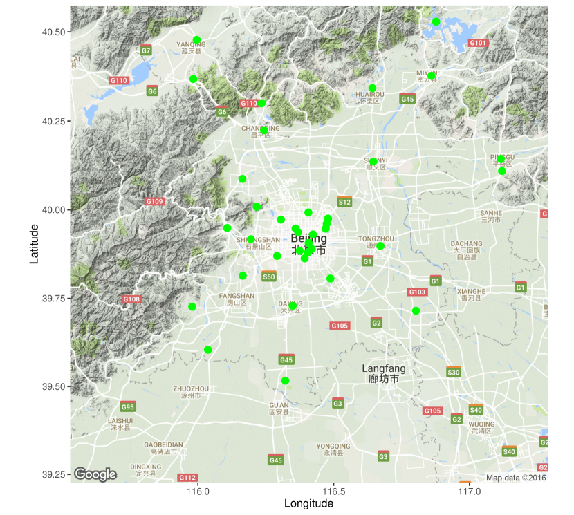
Figure 1: Map of the 36 PM_2.5 monitoring stations in Beijing

Example 1. With the rapid economic growth in China in recent years, there has also been a substantial increase in energy consumption, leading to serious air pollution in large part of China (Wang et al., 2002, 2015). One of the important pollution indicators is the so-called $\mbox{PM}_{2.5}$ index, which measures the concentration level of fine particulate matter in the air. The $\mbox{PM}_{2.5}$ pollution is severe in the north China plain (i.e., Beijing, Tianjin, and Hebei province). We consider here the hourly $\mbox{PM}_{2.5}$ readings at the 36 monitoring stations in Beijing area in the period of 1 April — 30 June 2016 (i.e., $n=2184,p=36$). Fig.1 is the map of those 36 stations. Fig.3 displays the original hourly $\mbox{PM}_{2.5}$ records from three randomly selected stations (i.e., Miyun, Huairou, and Shunyi). We apply the logarithmic transformation to the data and substract the mean for each of the 36 transformed series. Fig.3 plots the three transformed series from those in Fig.3. To fit model (2.1) to the transformed data, the 36 monitoring stations need to be arranged in a unilateral order. We consider the five possible options for the ordering, i.e., we order the stations along the directions from north to south, from west to east, from northwest to southeast, from northeast to southwest, and we also order the stations according to their geographic distances to Miyun – a station at the northeast corner of the region; see Fig.1. We select an ordering, among those five, according to a version of moving-window cross validation method; see below.

For each given ordering, we apply the ratio-based method to estimate the bandwidth parameter $k_{0}$. We apply a moving-window cross-validation scheme to calculate the post-sample predictive errors, i.e. for each of $t=2001,\cdots,2184$, we fit a model using only its 2000 immediate past observations. We then calculate one-step ahead and two-step ahead predictive errors. The results are summarized in Table 4. Based on both the one-step ahead and two-step ahead mean squared predictive errors, the ordering from west to east is preferred with the ordering from north to south as the close second. Note that for both of the orderings, the estimated bandwidth parameter is $\widehat{k}=5$.

According to the Air Quality Standard in China, the $\mbox{PM}_{2.5}$ pollution is marked at 7 different levels: Level 1 indicates the lowest pollution with the $\mbox{PM}_{2.5}$ concentration below 35 micrograms per cubic meter of air, and Level 7 corresponds to the worst scenarios with the $\mbox{PM}_{2.5}$ concentration exceeding 500 micrograms per cubic meter of air. For general public the prediction for the pollution level is of more interest than that for a concrete concentration value. Table 5 presents the percentages of the corrected one-step ahead and two-step ahead (post-sample) predictions at each of the 7 levels based on the five different orderings. It is easy to see from Table 5 that the higher the pollution level is, the more accurate the prediction is. Especially Level 6 and 7 pollution can always be correctly predicted based on all the five models. The preferred models with the ordering from north to south or from west to east provide overall higher percentages of correct prediction across the 7 pollution levels than the other three models.

Example 2. Now we consider the annual mortality rates in the period of 1872 — 2009 for the Italian population at age $i$, for $i=10,11,\cdots,50$. The data were downloaded from http://www.mortality.org/. Let $m_{i,t}$ be the original mortality rate (male and female in total) at age $i$ in the $t$-th year. Fig.4 displays the three series of $m_{i,t}$ with age $i=10,30,$ and $50$ respectively. Overall the mortality rates decrease for all age groups over the years except in the period of World War I in 1914 – 1918 and World War II in 1939 – 1945. Let $\{y_{i,t},t=1872,\cdots,2009\}$ be the centered log-scaled mortality rates for the $i$-th age group, $i=10,11,\cdots,50$. Thus $p=41$ and $n=138$. This orders the components of ${\mathbf{y}}_{t}$ naturally by the age. The ratio-based method leads to the estimated bandwidth parameter $\widehat{k}=1$ for this data set. We compute both one-step ahead and two-step ahead post-sample predictive errors for the last 8 data points for each of 41 series. The results are reported in Table 6.

Also included in Table 6 are the predictive errors based on the spatio-temporal model of Dou et al. (2016) which uses a known spatial weight matrix but with different scalar parameters for different location. The spatial weight matrix is defined as $W=(w_{i,j})$ with $w_{i,j}=a_{i,j}/\sum_{i}a_{i,j}$ for $i\neq j$, and 0 for $i=j$. We use two specifications for $a_{i,j}$: (i) a distance measure $a_{i,j}=(1+|i-j|)^{-1}$, and (ii) a correlation measure with $a_{i,j}$ taken as the absolute sample correlation between $y_{i,t}$ and $y_{j,t}$. Table 6 indicates clearly that the proposed banded model performs better than Dou et al. (2016)’s model in post-sample forecasting.

5 Concluding remarks

We propose in this paper a new class of banded spatio-temporal models. The setting does not require pre-specified spatial weight matrices. The coefficient matrices are estimated by a generalized method of moments estimation based on a Yule-Walker equation. The bandwidth of the coefficient matrices is determined by a ratio-based method.

Acknowledgments

We are grateful to the Editors and the anonymous referees for their insightful comments and suggestions that have substantially improved the presentation and the content of this paper. We also acknowledge the partial support of China’s National Key Research Special Program Grant 2016YFC0207702, National Natural Science Foundation of China (NSFC, 71532001, 11525101), Science Foundation of Ministry of Education of China 17YJC910006, and the UK EPSRC research grant EP/L01226X/1.

Appendix: Proofs

We present the proofs for Theorem 1 and Theorem 2 in this appendix. The idea of the proof for Theorem 2 is similar to that in Dou et al. (2016), but our setting is different since we have a banded structure and the convergence is a multivariate case. The proof for Theorem 4 follows directly from that of Theorem 2 and the proof for Theorem 3 is similar and simpler than that of Theorem 2, and they are therefore omitted. We use $C$ to denote a generic positive constant, which may be different at different places.

Before we prove the main theorems for the estimators in Section 2, we first give a lemma showing that the process $\{{\mathbf{y}}_{t}\}$ is strongly mixing under some regularity conditions.

Lemma 1.

If Conditions A1 and A2(a) hold, the process ${\mathbf{y}}_{t}$ is $\alpha-$mixing with the mixing coefficients $\alpha_{p}(k)$, defined in (3.1), satisfying the condition $\sum_{k=1}^{\infty}\alpha_{p}(k)^{\frac{\gamma}{4+\gamma}}<\infty$ uniformly for all sufficiently large $p$ and some constant $\gamma>0$.

Proof: It suffices to show that, uniformly for sufficiently large $p$, $\alpha_{p}(k)=O(a^{k})$ for $k\geq 1$ and some constant $a\in(0,1)$. Let

$${\mathbf{D}}=({\mathbf{I}}_{p}-{\mathbf{A}})^{-1}{\mathbf{B}}\,\,\text{and}\,\,\boldsymbol{\xi}_{t}=({\mathbf{I}}_{p}-{\mathbf{A}})^{-1}\mbox{\boldmath$\varepsilon$}_{t},$$

where $\boldsymbol{\xi}_{t}$ is the same with that in Condition A2. It follows from (2.3) and Condition A1 that

$$\mathbf{y}_{t}={\mathbf{D}}\mathbf{y}_{t-1}+\boldsymbol{\xi}_{t}=\sum_{k=0}^{\infty}{\mathbf{D}}^{k}\boldsymbol{\xi}_{t-k},$$ (A.1)

where ${\mathbf{D}}^{0}={\mathbf{I}}_{p}$. Note that the results of Lemmas 2.1-2.2 in Pham and  Tran (1985) are still valid for model (A.1) under assumptions A1-A2(a). To avoid the confusion of the notation $\alpha(j)$ in Pham and  Tran (1985), here we define $\sigma(j)=\sum_{k\geq j}\|{\mathbf{D}}^{k}\|_{2}$ to replace the expression of $\alpha(j)$ in their paper. By Lemmas 2.1-2.2 and the proof of Theorem 2.1 therein, we have

$$\|\Delta_{n}\|_{L^{1}}\leq C\sum_{j=n}^{\infty}\sigma(j)c_{j}+2\sum_{j=n}^{\infty}P(\|\boldsymbol{\xi}_{t}\|_{2}>c_{j}),$$

where $\Delta_{n}(x)$ is defined as (1.1) in Pham and Tran (1985), $\|\Delta_{n}\|_{L^{1}}$ is the $L^{1}$-norm of $\Delta_{n}(x)$ and $C$ is a generic constant independent of $p$. Let $c_{j}=p^{\delta/[2(1+\delta)]}\sigma(j)^{-1/(1+\delta)}$, by assumptions A1-A2(a) and Schwartz inequality, we have $P(\|\boldsymbol{\xi}_{t}\|_{2}>c_{j})\leq E\|\boldsymbol{\xi}_{t}\|_{2}^{\delta}/c_{j}^{\delta}$ and hence

$$\|\Delta_{n}\|_{L^{1}}\leq C\sum_{j=n}^{\infty}[\sum_{i=j}^{\infty}\rho^{i}]^{\delta/(1+\delta)}=O([\rho^{\delta/(1+\delta)}]^{n})=O(a^{n}),$$

where $a=\rho^{\delta/(1+\delta)}$. The conclusion of Lemma 1 follows from the fact that $\alpha_{p}(n)\leq 4\|\Delta_{n}\|_{L^{1}}$, see Pham and Tran (1985) for details. This completes the proof. $\Box$

Proof of Theorem 1. For each $i=1,...,p$, let $\widehat{k}_{i}=\mathop{\arg\max}_{1<k\leq K}(\mbox{RSS}_{i}(k-1)+w_{n})\big{/}(\mbox{RSS}_{i}(k)+w_{n})$. Our goal is to prove that $P(\widehat{k}=k_{0})\rightarrow 1.$ It is sufficient to show that

$$P(\widehat{k}<k_{0})\rightarrow 0\quad\textnormal{and}\quad P(\widehat{k}>k_{0})\rightarrow 0,$$ (A.2)

respectively. We first investigate the convergence rate of $\mbox{RSS}_{i}(k)$, which is crucial for proving the statement (A.2) above. For $k\geq k_{0}$, let

$$\widehat{\mathbf{V}}_{i,k}=({\mathbf{S}}_{i,k}^{(1)},\widehat{\boldsymbol{\Sigma}}^{\top}_{1,k_{0}},{\mathbf{S}}_{i,k}^{(2)},{\mathbf{S}}_{i,k}^{(3)},\widehat{\boldsymbol{\Sigma}}_{0,k_{0}},{\mathbf{S}}_{i,k}^{(4)}),\quad\boldsymbol{\beta}_{i,k}=({\mathbf{a}}_{i,k}^{(1)^{\top}},{\mathbf{a}}_{i,k_{0}}^{\top},{\mathbf{a}}_{i,k}^{(2)^{\top}},{\mathbf{b}}_{i,k}^{(1)^{\top}},{\mathbf{b}}_{i,k_{0}}^{\top},{\mathbf{b}}_{i,k}^{(2)^{\top}})^{\top},$$

where $\widehat{\mathbf{V}}_{i,k_{0}}=\widehat{\mathbf{V}}_{i}=(\widehat{\boldsymbol{\Sigma}}^{\top}_{1,k_{0}},\widehat{\boldsymbol{\Sigma}}_{0,k_{0}})$ and $\boldsymbol{\beta}_{i,k_{0}}=\boldsymbol{\beta}_{i}=({\mathbf{a}}_{i,k_{0}}^{\top},{\mathbf{b}}_{i,k_{0}}^{\top})^{\top}$, which correspond to the $\tau_{i}$ columns of $(\widehat{\boldsymbol{\Sigma}}_{1}^{\top},\widehat{\boldsymbol{\Sigma}}_{0})$ and $\tau_{i}$ non-zero elements of $({\mathbf{a}}_{i}^{\top},{\mathbf{b}}_{i}^{\top})^{\top}$, respectively. Define ${\mathbf{H}}_{i,k}=\widehat{\mathbf{V}}_{ik}(\widehat{\mathbf{V}}_{i,k}^{\top}\widehat{\mathbf{V}}_{i,k})^{-1}\widehat{\mathbf{V}}_{i,k}^{\top}$, it follows from (2.10) and (2.11) that

$$\mbox{RSS}_{i}(k_{0})=\frac{1}{p}\|({\mathbf{I}}-{\mathbf{H}}_{i,k_{0}})\frac{1}{n}\sum_{t=1}^{n}{\mathbf{y}}_{t-1}{{\varepsilon}}_{i,t}\|_{2}^{2}\leq\frac{1}{p}\|{\mathbf{I}}-{\mathbf{H}}_{i,k_{0}}\|_{2}^{2}\|\frac{1}{n}\sum_{t=1}^{n}{\mathbf{y}}_{t-1}{{\varepsilon}}_{i,t}\|_{2}^{2}.$$ (A.3)

Since $({\mathbf{I}}-{\mathbf{H}}_{i,k_{0}})^{2}={\mathbf{I}}-{\mathbf{H}}_{i,k_{0}}$ is a projection matrix, we have $\|{\mathbf{I}}-{\mathbf{H}}_{i,k_{0}}\|_{2}^{2}\leq 1$. Then, by a similar argument as (14) in Dou et al. (2016) or (A.22) below in the proof of Theorem 2, we conclude that

$$\mbox{RSS}_{i}(k_{0})\leq\frac{1}{p}\|\frac{1}{n}\sum_{t=1}^{n}{\mathbf{y}}_{t-1}{{\varepsilon}}_{i,t}\|_{2}^{2}=O_{p}(\frac{1}{n}).$$ (A.4)

When $k>k_{0}$, (2.10) can be rewritten as

$$\mbox{RSS}_{i}(k)=\frac{1}{p}\min_{{\mathbf{v}}_{1},{\mathbf{v}}_{2}}\|\widehat{\mathbf{z}}_{i}-\widehat{\mathbf{V}}_{i,k_{0}}{\mathbf{v}}_{1}-{\mathbf{S}}_{i,k}{\mathbf{v}}_{2}\|_{2}^{2},$$

where ${\mathbf{S}}_{i,k}=({\mathbf{S}}_{i,k}^{(1)},{\mathbf{S}}_{i,k}^{(2)},{\mathbf{S}}_{i,k}^{(3)},{\mathbf{S}}_{i,k}^{(4)})$. Let $\widetilde{\mathbf{S}}_{i,k}=({\mathbf{I}}_{p}-{\mathbf{H}}_{i,k_{0}}){\mathbf{S}}_{i,k}$, it can be verified that

$$\mbox{RSS}_{i}(k)=\frac{1}{p}\|({\mathbf{I}}_{p}-{\mathbf{H}}_{i,k_{0}})\widehat{\mathbf{z}}_{i}\|_{2}^{2}-\frac{1}{p}\|\widetilde{\mathbf{S}}_{i,k}\widehat{\mathbf{v}}_{2}\|_{2}^{2}=\mbox{RSS}_{i}(k_{0})-\frac{1}{p}\|\widetilde{\mathbf{S}}_{i,k}\widehat{\mathbf{v}}_{2}\|_{2}^{2},$$

where $\widehat{\mathbf{v}}_{2}=(\widetilde{\mathbf{S}}_{i,k}^{\top}\widetilde{\mathbf{S}}_{i,k})^{-1}\widetilde{\mathbf{S}}_{i,k}^{\top}\widehat{\mathbf{z}}_{i}$. By (2.11) and (A.4), we have

$$\mbox{RSS}_{i}(k)= \mbox{RSS}_{i}(k_{0})-\frac{1}{p}\|\widetilde{\mathbf{S}}_{i,k}(\widetilde{\mathbf{S}}_{i,k}^{\top}\widetilde{\mathbf{S}}_{i,k})^{-1}\widetilde{\mathbf{S}}_{i,k}^{\top}\frac{1}{n}\sum_{t=1}^{n}{\mathbf{y}}_{t-1}{{\varepsilon}}_{i,t}\|_{2}^{2}$$

$$\leq O_{p}(\frac{1}{n})+\frac{1}{p}\|\widetilde{\mathbf{S}}_{i,k}(\widetilde{\mathbf{S}}_{i,k}^{\top}\widetilde{\mathbf{S}}_{i,k})^{-1}\widetilde{\mathbf{S}}_{i,k}^{\top}\|_{2}^{2}\|\frac{1}{n}\sum_{t=1}^{n}{\mathbf{y}}_{t-1}{{\varepsilon}}_{i,t}\|_{2}^{2}$$

$$= O_{p}(\frac{1}{n}),$$ (A.5)

since $\widetilde{\mathbf{S}}_{i,k}(\widetilde{\mathbf{S}}_{i,k}^{\top}\widetilde{\mathbf{S}}_{i,k})^{-1}\widetilde{\mathbf{S}}_{i,k}^{\top}$ is a projection matrix.

Similarly, for $k<k_{0}$, we define

$$\widehat{\mathbf{V}}_{i,k_{0}}=(\mathbf{J}_{i,k}^{(1)},\widehat{\boldsymbol{\Sigma}}^{\top}_{1,k},\mathbf{J}_{i,k}^{(2)},\mathbf{J}_{i,k}^{(3)},\widehat{\boldsymbol{\Sigma}}_{0,k_{0}},\mathbf{J}_{i,k}^{(4)}),\quad\boldsymbol{\beta}_{i,k_{0}}=(\mathbf{c}_{i,k}^{(1)^{\top}},{\mathbf{a}}_{i,k}^{\top},\mathbf{c}_{i,k}^{(2)^{\top}},\mathbf{d}_{i,k}^{(1)^{\top}},{\mathbf{b}}_{i,k}^{\top},\mathbf{d}_{i,k}^{(2)^{\top}})^{\top},$$

where $\widehat{\mathbf{V}}_{i,k}=(\widehat{\boldsymbol{\Sigma}}^{\top}_{1,k},\widehat{\boldsymbol{\Sigma}}_{0,k})$ and $\boldsymbol{\beta}_{i,k=}({\mathbf{a}}_{i,k}^{\top},{\mathbf{b}}_{i,k}^{\top})^{\top}$, which correspond to $\tau_{i}(k)$ columns of $(\widehat{\boldsymbol{\Sigma}}_{1}^{\top},\boldsymbol{\Sigma}_{0})$ and $\tau_{i}(k)$ elements of $\beta_{i}$. $\tau_{i}(k)$ is defined as (2.6) with $k_{0}$ replaced by $k$. It follows from (2.11) that

$$\widehat{\mathbf{z}}_{i}=\widehat{\mathbf{V}}_{i,k_{0}}\boldsymbol{\beta}_{i,k_{0}}+\frac{1}{n}\sum_{t=1}^{n}{\mathbf{y}}_{t-1}{{\varepsilon}}_{i,t}=\widehat{\mathbf{V}}_{i,k}\boldsymbol{\beta}_{i,k}+\mathbf{J}_{i,k}\mathbf{\delta}_{i,k}+\frac{1}{n}\sum_{t=1}^{n}{\mathbf{y}}_{t-1}{{\varepsilon}}_{i,t},$$ (A.6)

where $\mathbf{J}_{i,k}=(\mathbf{J}_{i,k}^{(1)},\mathbf{J}_{i,k}^{(2)},\mathbf{J}_{i,k}^{(3)},\mathbf{J}_{i,k}^{(4)})$ and $\mathbf{\delta}_{i,k}=(\mathbf{c}_{i,k}^{(1)^{\top}},\mathbf{c}_{i,k}^{(2)^{\top}},\mathbf{d}_{i,k}^{(1)^{\top}},\mathbf{d}_{i,k}^{(2)^{\top}})^{\top}$. By (2.10) and (A.6),

$$\mbox{RSS}_{i}(k)= \frac{1}{p}\|({\mathbf{I}}_{p}-{\mathbf{H}}_{i,k})\widehat{\mathbf{z}}_{i}\|_{2}^{2}$$

$$= \frac{1}{p}\|({\mathbf{I}}-{\mathbf{H}}_{i,k})\mathbf{J}_{i,k}\mathbf{\delta}_{i,k}+({\mathbf{I}}-{\mathbf{H}}_{i,k})\frac{1}{n}\sum_{t=1}^{n}{\mathbf{y}}_{t-1}{{\varepsilon}}_{i,t}\|_{2}^{2}$$

$$= \frac{1}{p}\|({\mathbf{I}}-{\mathbf{H}}_{i,k})\mathbf{J}_{i,k}\mathbf{\delta}_{i,k}\|_{2}^{2}+\frac{1}{p}\|({\mathbf{I}}-{\mathbf{H}}_{i,k})\frac{1}{n}\sum_{t=1}^{n}{\mathbf{y}}_{t-1}{{\varepsilon}}_{i,t}\|_{2}^{2}$$

$$+\frac{2}{p}\mathbf{\delta}_{i,k}^{\top}\mathbf{J}_{i,k}^{\top}({\mathbf{I}}-{\mathbf{H}}_{i,k})\frac{1}{n}\sum_{t=1}^{n}{\mathbf{y}}_{t-1}{{\varepsilon}}_{i,t}.$$ (A.7)

By Condition A5, we have

$$\lambda_{\min}\{\mathbf{J}_{i,k}^{\top}({\mathbf{I}}_{p}-{\mathbf{H}}_{i,k})\mathbf{J}_{i,k}\}\geq\lambda_{1}\quad\text{and}\quad\lambda_{\max}\{\mathbf{J}_{i,k}^{\top}({\mathbf{I}}_{p}-{\mathbf{H}}_{i,k})\mathbf{J}_{i,k}\}\leq\lambda_{2}.$$

Then, the first term of (Appendix: Proofs) can be bounded by

$$\frac{\lambda_{1}}{p}(a_{i,i-k_{0}}^{2}+a_{i,i+k_{0}}^{2}+b_{i,i-k_{0}}^{2}+b_{i,i+k_{0}}^{2})\leq\frac{1}{p}\|({\mathbf{I}}-{\mathbf{H}}_{i,k})\mathbf{J}_{i,k}\mathbf{\delta}_{i,k}\|_{2}^{2}\leq\frac{\lambda_{2}}{p}\|\boldsymbol{\beta}_{i,k_{0}}\|_{2}^{2}.$$ (A.8)

By Conditions A6 and A7, (A.8) can be relaxed to

$$\frac{C_{n}k_{0}\lambda_{1}\log(p\vee n)}{np}\leq\frac{1}{p}\|({\mathbf{I}}-{\mathbf{H}}_{i,k})\mathbf{J}_{i,k}\mathbf{\delta}_{i,k}\|_{2}^{2}\leq\frac{O(1)\lambda_{2}}{p}.$$ (A.9)

The second term is of order $O_{p}(\frac{1}{n})$ by (A.4). By Cauchy-Schwarz inequality, the third term can be bounded by the sum of the first and the second terms. As a result,

$$\frac{C_{n}k_{0}\lambda_{1}\log(p\vee n)}{np}+O_{p}(\frac{1}{n})\leq\mbox{RSS}_{i}(k)\leq\frac{O(1)\lambda_{2}}{p}.$$ (A.10)

Now we are able to prove (A.2). To prove $P(\widehat{k}>k_{0})\rightarrow 0$, we note that $P(\widehat{k}>k_{0})\leq P(\widehat{k}_{i}>k_{0})$ for some $i\in\{1,...,p\}$ and the event $\{\widehat{k}_{i}>k_{0}\}$ implies

$$A_{in}\equiv\{\max\limits_{k>k_{0}}\frac{\mbox{RSS}_{i}(k-1)+w_{n}}{\mbox{RSS}_{i}(k)+w_{n}}>\frac{\mbox{RSS}_{i}(k_{0}-1)+w_{n}}{\mbox{RSS}_{i}(k_{0})+w_{n}}\}.$$

Then, we only need to show that $P(A_{in})\rightarrow 0$ for some $i$. By (Appendix: Proofs), (A.10) and Condition A5,

$$\frac{\mbox{RSS}_{i}(k_{0}-1)+w_{n}}{\mbox{RSS}_{i}(k_{0})+w_{n}}\geq\frac{\lambda_{1}C_{n}k_{0}\log(p\vee n)/(np)}{O_{p}(1/n)}\rightarrow\infty,$$ (A.11)

and

$$\max\limits_{k>k_{0}}\frac{\mbox{RSS}_{i}(k-1)+w_{n}}{\mbox{RSS}_{i}(k)+w_{n}}\leq\frac{w_{n}+O_{p}(1/n)}{w_{n}}=O_{p}(1).$$ (A.12)

It follows from (A.11) and (A.12) that $P(A_{in})\rightarrow 0$, and hence $P(\widehat{k}>k_{0})\rightarrow 0$.

Similarly, to prove $P(\widehat{k}<k_{0})\rightarrow 0$, we only need to show that $P(B_{in})\rightarrow 0$ for some $i\in\{1,...,p\}$, where

$$B_{in}\equiv\{\max\limits_{k<k_{0}}\frac{\mbox{RSS}_{i}(k-1)+w_{n}}{\mbox{RSS}_{i}(k)+w_{n}}>\frac{\mbox{RSS}_{i}(k_{0}-1)+w_{n}}{\mbox{RSS}_{i}(k_{0})+w_{n}}\}.$$

By (A.10),

$$\max\limits_{k<k_{0}}\frac{\mbox{RSS}_{i}(k-1)+w_{n}}{\mbox{RSS}_{i}(k)+w_{n}}\leq\frac{w_{n}+O_{p}(1)\lambda_{2}/p}{{C_{n}k_{0}\lambda_{1}\log(p\vee n)/(np)}+O_{p}(1/n)}.$$ (A.13)

We now compare the ratio between the upper bound of (A.13) and the lower bound of (A.11),

$$\left\{\frac{w_{n}+O_{p}(1)\lambda_{2}/p}{{C_{n}k_{0}\lambda_{1}\log(p\vee n)/(np)}+O_{p}(1/n)}\right\}\bigg{/}\left\{\frac{\lambda_{1}C_{n}k_{0}\log(p\vee n)/(np)}{O_{p}(1/n)}\right\}$$

$$=\frac{O_{p}(p^{2})+O_{p}(np)}{O_{p}(C_{n}^{2}(\log(p\vee n))^{2})+O_{p}(pC_{n}\log(p\vee n))}\rightarrow 0,$$ (A.14)

as long as $C_{n}^{2}/(np)\rightarrow\infty$. It follows from (A.11), (A.13) and (Appendix: Proofs) that $P(B_{in})\rightarrow 0$. If $k_{0}$ is not fixed, the upper bound in (A.10) can be replaced by $O(1)k_{0}\lambda_{2}/p$, (Appendix: Proofs) still holds under Conditions A4-A6. This completes the proof of Theorem 1. $\Box$

Proof of Theorem 2. By Theorem 1, with probability tending to one, $\widehat{k}=k_{0}$, and thus it suffices to consider the set $\mathcal{A}_{n}=\{\widehat{k}=k_{0}\}$. Over the set $\mathcal{A}_{n}$, to prove part $(i)$ of Theorem 2 for a fixed $k_{0}$, following the same arguments in Dou et al. (2016), we only need to verify the assertions (1) and (2) below.

• $$\sqrt{n}{\mathbf{U}}_{i}^{-\frac{1}{2}}\widehat{\mathbf{V}}_{i}^{\top}\left(\frac{1}{n}\sum_{t=2}^{n}{\mathbf{y}}_{t-1}{{\varepsilon}}_{i,t}\right) =\sqrt{n}{\mathbf{U}}_{i}^{-\frac{1}{2}}\left(\begin{array}[]{l}\frac{1}{n}\sum_{t=2}^{n}(y_{j,t})_{j\in S_{i}}{\mathbf{y}}^{\top}_{t-1}\left(\frac{1}{n}\sum_{t=2}^{n}{\mathbf{y}}_{t-1}{{\varepsilon}}_{i,t}\right)\\ \frac{1}{n}\sum_{t=2}^{n}(y_{j,t-1})_{j\in S_{i}^{+}}{\mathbf{y}}^{\top}_{t-1}\left(\frac{1}{n}\sum_{t=2}^{n}{\mathbf{y}}_{t-1}{{\varepsilon}}_{i,t}\right)\end{array}\right)$$

  $$\rightarrow_{d}N(0,{\mathbf{I}}_{\tau_{i}}).$$

• ${\mathbf{K}}_{i}(\widehat{\mathbf{V}}_{i}^{\top}\widehat{\mathbf{V}}_{i})^{-1}\rightarrow_{p}{\mathbf{I}}_{\tau_{i}}.$

To prove assertion (1), it suffices to show that for any nonzero vector $\mathbf{u}=(\mathbf{u}_{1}^{\top},\mathbf{u}_{2}^{\top})^{\top}\in\mathbb{R}^{\tau_{i}}$, where $\mathbf{u}_{1}\in\mathbb{R}^{S_{i}}$, $\mathbf{u}_{2}\in\mathbb{R}^{S_{i}^{+}}$ and $\tau_{i}=|S_{i}|+|S_{i}^{+}|$, the linear combination

$$\sqrt{n}{\mathbf{u}}^{\top}\left(\begin{array}[]{l}\frac{1}{n}\sum_{t=2}^{n}(y_{j,t})_{j\in S_{i}}{\mathbf{y}}^{\top}_{t-1}\left(\frac{1}{n}\sum_{t=2}^{n}{\mathbf{y}}_{t-1}{{\varepsilon}}_{i,t}\right)\\ \frac{1}{n}\sum_{t=2}^{n}(y_{j,t-1})_{j\in S_{i}^{+}}{\mathbf{y}}^{\top}_{t-1}\left(\frac{1}{n}\sum_{t=2}^{n}{\mathbf{y}}_{t-1}{{\varepsilon}}_{i,t}\right)\end{array}\right)$$ (A.20)

is asymptotically normal. Let us consider one term in the upper block of (A.20) first. For each $j\in S_{i}$, we have

$$\frac{1}{n}\sum_{t=2}^{n}y_{j,t}{\mathbf{y}}^{\top}_{t-1}(\frac{1}{n}\sum_{t=2}^{n}{\mathbf{y}}_{t-1}{{\varepsilon}}_{i,t})= \frac{1}{n}\sum_{t=2}^{n}(y_{j,t}{\mathbf{y}}^{\top}_{t-1}-E(y_{j,t}{\mathbf{y}}^{\top}_{t-1}))\frac{1}{n}\sum_{t=2}^{n}{\mathbf{y}}_{t-1}{{\varepsilon}}_{i,t}$$

$$+\frac{n-1}{n}E(y_{j,t}{\mathbf{y}}^{\top}_{t-1})\frac{1}{n}\sum_{t=2}^{n}{\mathbf{y}}_{t-1}{{\varepsilon}}_{i,t}$$

$$=\frac{1}{n}\sum_{t=2}^{n}({\mathbf{e}}_{j}^{\top}{\mathbf{y}}_{t}{\mathbf{y}}^{\top}_{t-1}-{\mathbf{e}}_{j}^{\top}\boldsymbol{\Sigma}_{1})\frac{1}{n}\sum_{t=2}^{n}{\mathbf{y}}_{t-1}{{\varepsilon}}_{i,t}$$

$$+\frac{n-1}{n}{\mathbf{e}}_{j}^{\top}\boldsymbol{\Sigma}_{1}\frac{1}{n}\sum_{t=2}^{n}{\mathbf{y}}_{t-1}{{\varepsilon}}_{i,t}$$

$$=E_{1}+E_{2}.$$ (A.21)

By a similar argument as (14) in Dou et al. (2016), we can show that

$$E_{1}=O_{p}(\frac{p}{n})\quad\text{and}\quad E_{2}=O_{p}(\frac{1}{\sqrt{n}}).$$ (A.22)

If $p=o(\sqrt{n})$, it follows that

$$\frac{1}{n}\sum_{t=2}^{n}y_{j,t}{\mathbf{y}}^{\top}_{t-1}(\frac{1}{\sqrt{n}}\sum_{t=2}^{n}{\mathbf{y}}_{t-1}{{\varepsilon}}_{i,t})={\mathbf{e}}_{j}^{\top}\boldsymbol{\Sigma}_{1}\frac{1}{\sqrt{n}}\sum_{t=2}^{n}{\mathbf{y}}_{t-1}{{\varepsilon}}_{i,t}+o_{p}(1),\quad j\in S_{i}.$$ (A.23)

Similarly, we can show that

$$\frac{1}{n}\sum_{t=2}^{n}y_{j,t-1}{\mathbf{y}}^{\top}_{t-1}(\frac{1}{\sqrt{n}}\sum_{t=2}^{n}{\mathbf{y}}_{t-1}{{\varepsilon}}_{i,t})={\mathbf{e}}_{j}^{\top}\boldsymbol{\Sigma}_{0}\frac{1}{\sqrt{n}}\sum_{t=2}^{n}{\mathbf{y}}_{t-1}{{\varepsilon}}_{i,t}+o_{p}(1),\quad j\in S_{i}^{+}.$$ (A.24)

Now it suffices to prove

$$S_{n,p}\equiv\mathbf{u}_{1}^{T}{\mathbf{I}}_{S_{i}}^{\top}\boldsymbol{\Sigma}_{1}\frac{1}{\sqrt{n}}\sum_{t=2}^{n}{\mathbf{y}}_{t-1}{{\varepsilon}}_{i,t}+\mathbf{u}_{2}^{\top}{\mathbf{I}}_{S_{i}^{+}}^{\top}\boldsymbol{\Sigma}_{0}\frac{1}{\sqrt{n}}\sum_{t=2}^{n}{\mathbf{y}}_{t-1}{{\varepsilon}}_{i,t}$$

is asymptotically normal, where ${\mathbf{I}}_{S_{i}}$ and ${\mathbf{I}}_{S_{i}^{+}}$ are defined as those in (3.6).

Now we calculate the variance of $S_{n,p}$. It holds that

$$\textnormal{Var}(\mathbf{u}_{1}^{T}{\mathbf{I}}_{S_{i}}^{\top}\boldsymbol{\Sigma}_{1}\frac{1}{\sqrt{n}}\sum_{t=2}^{n}{\mathbf{y}}_{t-1}{{\varepsilon}}_{i,t})= \mathbf{u}_{1}^{T}{\mathbf{I}}_{S_{i}}^{\top}\boldsymbol{\Sigma}_{1}\frac{n-1}{n}\boldsymbol{\Sigma}_{\mathbf{y},\mbox{\boldmath$\varepsilon$}_{i}}(0)\boldsymbol{\Sigma}_{1}^{\top}{\mathbf{I}}_{S_{i}}{\mathbf{u}}_{1}$$ (A.25)

$$+{\mathbf{u}}_{1}^{\top}{\mathbf{I}}_{S_{i}}^{\top}\boldsymbol{\Sigma}_{1}\sum_{j=1}^{n-2}(1-\frac{j+1}{n})[\boldsymbol{\Sigma}_{{\mathbf{y}},\mbox{\boldmath$\varepsilon$}_{i}}(j)+\boldsymbol{\Sigma}^{\top}_{{\mathbf{y}},\mbox{\boldmath$\varepsilon$}_{i}}(j)]\boldsymbol{\Sigma}_{1}^{\top}{\mathbf{I}}_{S_{i}}{\mathbf{u}}_{1}.$$

We note that

$$E|{\mathbf{e}}_{j}^{\top}\boldsymbol{\Sigma}_{1}{\mathbf{y}}_{t-1}{{\varepsilon}}_{i,t}|^{\frac{4+\gamma}{2}}\leq[E|{\mathbf{e}}_{j}^{\top}\boldsymbol{\Sigma}_{1}{\mathbf{y}}_{t-1}|^{4+\gamma}]^{\frac{1}{2}}[E|{{\varepsilon}}_{i,t}|^{4+\gamma}]^{\frac{1}{2}}\leq\infty.$$

By Proposition 2.5 of Fan and Yao (2003), it follows from $\sum_{j=1}^{\infty}\alpha_{p}(j)^{\frac{\gamma}{4+\gamma}}<\infty$ in Lemma 1 that

$$\mathop{\sup}_{p} \sum_{j=1}^{\infty}|{\mathbf{u}}_{1}^{\top}{\mathbf{I}}_{S_{i}}^{\top}\boldsymbol{\Sigma}_{1}[\boldsymbol{\Sigma}_{{\mathbf{y}},\mbox{\boldmath$\varepsilon$}_{i}}(j)+\boldsymbol{\Sigma}_{{\mathbf{y}},\mbox{\boldmath$\varepsilon$}_{i}}^{\top}(j)]\boldsymbol{\Sigma}_{1}^{\top}{\mathbf{I}}_{S_{i}}{\mathbf{u}}_{1}|$$

$$\leq C\mathop{\sup}_{j_{1},j_{2}\leq p}\sum_{j=1}^{\infty}|{\mathbf{e}}_{j_{1}}^{\top}\boldsymbol{\Sigma}_{1}\boldsymbol{\Sigma}_{{\mathbf{y}},\mbox{\boldmath$\varepsilon$}_{i}}(j)\boldsymbol{\Sigma}_{1}^{\top}{\mathbf{e}}_{j_{2}}|$$

$$\leq C\mathop{\sup}_{l\leq p}\sum_{j=1}^{\infty}\alpha_{p}(j)^{\frac{\gamma}{4+\gamma}}(E|{\mathbf{e}}_{l}^{\top}\boldsymbol{\Sigma}_{1}{\mathbf{y}}_{t-1}|^{4+\gamma})^{\frac{2}{4+\gamma}}(E|{{\varepsilon}}_{i,t}|^{4+\gamma})^{\frac{2}{4+\gamma}}\;<\;\infty.$$

Similarly,

Cov $$\left(\mathbf{u}_{1}^{T}{\mathbf{I}}_{S_{i}}^{\top}\boldsymbol{\Sigma}_{1}\frac{1}{\sqrt{n}}\sum_{t=2}^{n}{\mathbf{y}}_{t-1}{{\varepsilon}}_{i,t},\mathbf{u}_{2}^{\top}{\mathbf{I}}_{S_{i}^{+}}^{\top}\boldsymbol{\Sigma}_{0}\frac{1}{\sqrt{n}}\sum_{t=2}^{n}{\mathbf{y}}_{t-1}{{\varepsilon}}_{i,t}\right)$$

$$= \mathbf{u}_{1}^{T}{\mathbf{I}}_{S_{i}}^{\top}\boldsymbol{\Sigma}_{1}\frac{n-1}{n}\boldsymbol{\Sigma}_{\mathbf{y},\mbox{\boldmath$\varepsilon$}_{i}}(0)\boldsymbol{\Sigma}_{0}{\mathbf{I}}_{S_{i}^{+}}{\mathbf{u}}_{2}$$

$$+{\mathbf{u}}_{1}^{\top}{\mathbf{I}}_{S_{i}}^{\top}\boldsymbol{\Sigma}_{1}\sum_{j=1}^{n-2}(1-\frac{j+1}{n})[\boldsymbol{\Sigma}_{{\mathbf{y}},\mbox{\boldmath$\varepsilon$}_{i}}(j)+\boldsymbol{\Sigma}^{\top}_{{\mathbf{y}},\mbox{\boldmath$\varepsilon$}_{i}}(j)]\boldsymbol{\Sigma}_{0}{\mathbf{I}}_{S_{i}^{+}}{\mathbf{u}}_{2},$$

and $\sup_{p}\sum_{j=1}^{\infty}|{\mathbf{u}}_{1}^{\top}{\mathbf{I}}_{S_{i}}^{\top}\boldsymbol{\Sigma}_{1}[\boldsymbol{\Sigma}_{{\mathbf{y}},\mbox{\boldmath$\varepsilon$}_{i}}(j)+\boldsymbol{\Sigma}_{{\mathbf{y}},\mbox{\boldmath$\varepsilon$}_{i}}^{\top}(j)]\boldsymbol{\Sigma}_{0}{\mathbf{I}}_{S_{i}^{+}}{\mathbf{u}}_{2}|<\infty$. Calculating all the variance and covariance and summing them up, it follows from dominate convergence theorem that

$$\textnormal{Var}\left(\frac{S_{n,p}}{\sqrt{\mathbf{u}^{\top}{\mathbf{U}}_{i}\mathbf{u}}}\right)\rightarrow 1.$$

To prove the asymptotic normality of $S_{n,p}$, we can employ the small-block and large-block arguments as those in Dou et al. (2016). We will borrow the notations $k_{n}$, $s_{n}$ and $l_{n}$ from their paper with the same properties and briefly introduce the steps for our case.

We can partition $S_{n,p}$ in the following way

$$S_{n,p}= \mathbf{u}_{1}^{\top}\frac{1}{\sqrt{n}}\sum_{j=1}^{k_{n}}\xi_{j}^{(1)}+\mathbf{u}_{2}^{\top}\frac{1}{\sqrt{n}}\sum_{j=1}^{k_{n}}\xi_{j}^{(2)}+\mathbf{u}_{1}^{\top}\frac{1}{\sqrt{n}}\sum_{j=1}^{k_{n}}\eta_{j}^{(1)}+\mathbf{u}_{2}^{\top}\frac{1}{\sqrt{n}}\sum_{j=1}^{k_{n}}\eta_{j}^{(2)}$$ (A.26)

$$\mathbf{u}_{1}^{\top}\frac{1}{\sqrt{n}}\zeta^{(1)}+\mathbf{u}_{2}^{\top}\frac{1}{\sqrt{n}}\zeta^{(2)},$$

where

$$\xi_{j}^{(1)}=\sum_{t=(j-1)(l_{n}+s_{n})+1}^{jl_{n}+(j-1)s_{n}}{\mathbf{I}}^{\top}_{S_{i}}\boldsymbol{\Sigma}_{1}{\mathbf{y}}_{t-1}{{\varepsilon}}_{i,t},\quad\eta_{j}^{(1)}=\sum_{t=jl_{n}+(j-1)s_{n}+1}^{j(l_{n}+s_{n})}{\mathbf{I}}^{\top}_{S_{i}}\boldsymbol{\Sigma}_{1}\mathbf{y}_{t-1}{{\varepsilon}}_{i,t},$$

$$\xi_{j}^{(2)}=\sum_{t=(j-1)(l_{n}+s_{n})+1}^{jl_{n}+(j-1)s_{n}}{\mathbf{I}}^{\top}_{S_{i}^{+}}\boldsymbol{\Sigma}_{0}{\mathbf{y}}_{t-1}{{\varepsilon}}_{i,t},\quad\eta_{j}^{(2)}=\sum_{t=jl_{n}+(j-1)s_{n}+1}^{j(l_{n}+s_{n})}{\mathbf{I}}^{\top}_{S_{i}^{+}}\boldsymbol{\Sigma}_{0}\mathbf{y}_{t-1}{{\varepsilon}}_{i,t},$$

$$\zeta^{(1)}=\sum_{t=k_{n}(l_{n}+s_{n})+1}^{n}{\mathbf{I}}^{\top}_{S_{i}}\boldsymbol{\Sigma}_{1}\mathbf{y}_{t-1}{{\varepsilon}}_{i,t},\quad\zeta^{(2)}=\sum_{t=k_{n}(l_{n}+s_{n})+1}^{n}{\mathbf{I}}^{\top}_{S_{i}^{+}}\boldsymbol{\Sigma}_{0}{\mathbf{y}}_{t-1}{{\varepsilon}}_{i,t},$$

and the summation starts from ${\mathbf{y}}_{0}$ for the convenience of calculation. Note that, $\xi_{j}^{(1)}$, $\eta_{j}^{(1)}$ and $\zeta_{j}^{(1)}$ are $|S_{i}|$ dimensional vectors, and $\xi_{j}^{(2)}$, $\eta_{j}^{(2)}$ and $\zeta_{j}^{(2)}$ are $|S_{i}^{+}|$ dimensional vectors. Since $\alpha_{p}(n)=o(n^{-\frac{(2+\gamma/2)2}{2(2+\gamma/2-2)}})$ and $k_{n}s_{n}/n\rightarrow 0$, $(l_{n}+s_{n})/n\rightarrow 0$, by applying Proposition 2.7 of Fan and Yao (2003), it holds that

$$\frac{1}{\sqrt{n}}\sum_{j=1}^{k_{n}}\eta_{j}^{(l)}=o_{p}(1)\quad\text{and}\quad\frac{1}{\sqrt{n}}\zeta^{(l)}=o_{p}(1),\quad l=1,2.$$ (A.27)

Therefore,

$$S_{n,p}=\mathbf{u}_{1}^{\top}\frac{1}{\sqrt{n}}\sum_{j=1}^{k_{n}}\xi_{j}^{(1)}+\mathbf{u}_{2}^{\top}\frac{1}{\sqrt{n}}\sum_{j=1}^{k_{n}}\xi_{j}^{(2)}+o_{p}(1)\equiv T_{n,p}+o_{p}(1).$$ (A.28)

Similar to (A.25), we can calculate the variance of $T_{n,p}$ and it holds that

$$\textnormal{Var}\left(\frac{T_{n,p}}{\sqrt{\mathbf{u}^{\top}{\mathbf{U}}_{i}\mathbf{u}}}\right)\rightarrow 1,$$ (A.29)

see also Dou et al. (2016) for a similar argument. Now, it suffices to prove the asymptotic normality of $T_{n,p}$. We partition $T_{n,p}$ into two parts via truncation. Specifically, we define

$$\xi_{j}^{(1)L}=\sum_{t=(j-1)(l_{n}+s_{n})+1}^{jl_{n}+(j-1)s_{n}}{\mathbf{I}}^{\top}_{S_{i}}\boldsymbol{\Sigma}_{1}\mathbf{y}_{t-1}{{\varepsilon}}_{i,t}{\mathbf{I}}_{\{\|{\mathbf{I}}^{\top}_{S_{i}}\boldsymbol{\Sigma}_{1}{\mathbf{y}}_{t-1}{{\varepsilon}}_{i,t}\|_{2}\leq L\}},$$

and

$$\xi_{j}^{(1)R}=\sum_{t=(j-1)(l_{n}+s_{n})+1}^{jl_{n}+(j-1)s_{n}}{\mathbf{I}}^{\top}_{S_{i}}\boldsymbol{\Sigma}_{1}{\mathbf{y}}_{t-1}{{\varepsilon}}_{i,t}{\mathbf{I}}_{\{\|{\mathbf{I}}^{\top}_{S_{i}}\boldsymbol{\Sigma}_{1}{\mathbf{y}}_{t-1}{{\varepsilon}}_{i,t}\|_{2}>L\}}.$$

Similarly, we can define $\xi_{j}^{(2)L}$ and $\xi_{j}^{(2)R}$. Then,

$$T_{n,p} = \left(\mathbf{u}_{1}^{T}\frac{1}{\sqrt{n}}\sum_{j=1}^{k_{n}}\xi_{j}^{(1)L}+\mathbf{u}_{2}^{T}\frac{1}{\sqrt{n}}\sum_{j=1}^{k_{n}}\xi_{j}^{(2)L}\right)+\left(\mathbf{u}_{1}^{T}\frac{1}{\sqrt{n}}\sum_{j=1}^{k_{n}}\xi_{j}^{(1)R}+\mathbf{u}_{2}^{T}\frac{1}{\sqrt{n}}\sum_{j=1}^{k_{n}}\xi_{j}^{(2)R}\right)$$ (A.30)

$$\equiv T_{n,p}^{L}+T_{n,p}^{R}.$$

Define

$$\boldsymbol{\Sigma}_{{\mathbf{y}},\mbox{\boldmath$\varepsilon$}_{i},L}^{(S_{i},S_{i}^{+})}(j)=\textnormal{Cov}(\mathbf{y}_{t-1+j}{{\varepsilon}}_{i,t+j}{\mathbf{I}}_{\{\|{\mathbf{I}}^{\top}_{S_{i}}\boldsymbol{\Sigma}_{1}{\mathbf{y}}_{t-1+j}{{\varepsilon}}_{i,t+j}\|_{2}\leq L\}},{\mathbf{y}}_{t-1}{{\varepsilon}}_{i,t}{\mathbf{I}}_{\{\|{\mathbf{I}}^{\top}_{S_{i}^{+}}\boldsymbol{\Sigma}_{0}\mathbf{y}_{t-1}{{\varepsilon}}_{i,t}\|_{2}\leq L\}})$$

for $j=0,1,2,...$, and

$$\boldsymbol{\Sigma}^{(S_{i},S_{i}^{+})}_{{\mathbf{y}},\mbox{\boldmath$\varepsilon$}_{i},L}=\boldsymbol{\Sigma}^{(S_{i},S_{i}^{+})}_{\mathbf{y},\mbox{\boldmath$\varepsilon$}_{i},L}(0)+\sum_{j=1}^{\infty}\left(\boldsymbol{\Sigma}^{(S_{i},S_{i}^{+})}_{{\mathbf{y}},\mbox{\boldmath$\varepsilon$}_{i},L}(j)+(\boldsymbol{\Sigma}^{(S_{i},S_{i}^{+})}_{{\mathbf{y}},\mbox{\boldmath$\varepsilon$}_{i},L}(j))^{\top}\right).$$

Similarly we have $\boldsymbol{\Sigma}^{(S_{i},S_{i})}_{{\mathbf{y}},\mbox{\boldmath$\varepsilon$}_{i},L}$, $\boldsymbol{\Sigma}^{(S_{i}^{+},S_{i})}_{{\mathbf{y}},\mbox{\boldmath$\varepsilon$}_{i},L}$ and $\boldsymbol{\Sigma}^{(S_{i}^{+},S_{i}^{+})}_{{\mathbf{y}},\mbox{\boldmath$\varepsilon$}_{i},L}$. Let

$${\mathbf{U}}_{i}^{L}\equiv\left(\begin{array}[]{ll}{\mathbf{I}}_{S_{i}}^{\top}\boldsymbol{\Sigma}_{1}\boldsymbol{\Sigma}^{(S_{i},S_{i})}_{{\mathbf{y}},\mbox{\boldmath$\varepsilon$}_{i},L}\boldsymbol{\Sigma}_{1}^{\top}{\mathbf{I}}_{S_{i}}&{\mathbf{I}}_{S_{i}}^{\top}\boldsymbol{\Sigma}_{1}\boldsymbol{\Sigma}^{(S_{i},S_{i}^{+})}_{{\mathbf{y}},\mbox{\boldmath$\varepsilon$}_{i},L}\boldsymbol{\Sigma}_{0}{\mathbf{I}}_{S_{i}^{+}}.\\ {\mathbf{I}}_{S_{i}^{+}}^{\top}\boldsymbol{\Sigma}_{0}\boldsymbol{\Sigma}^{(S_{i}^{+},S_{i})}_{{\mathbf{y}},\mbox{\boldmath$\varepsilon$}_{i},L}\boldsymbol{\Sigma}_{1}^{\top}{\mathbf{I}}_{S_{i}}&{\mathbf{I}}_{S_{i}^{+}}^{\top}\boldsymbol{\Sigma}_{0}\boldsymbol{\Sigma}^{(S_{i}^{+},S_{i}^{+})}_{{\mathbf{y}},\mbox{\boldmath$\varepsilon$}_{i},L}\boldsymbol{\Sigma}_{0}{\mathbf{I}}_{S_{i}^{+}}\end{array}\right).$$ (A.33)

Then ${\mathbf{U}}_{i}^{L}\rightarrow{\mathbf{U}}_{i}$ as $L\rightarrow\infty$. Similar to (A.29), it holds that

$$\textnormal{Var}\left(\frac{T_{n,p}^{L}}{\sqrt{\mathbf{u}^{\top}{\mathbf{U}}_{i}^{L}\mathbf{u}}}\right)\rightarrow 1.$$

If we define $U_{i}^{R}$ in a similar way, then $U_{i}^{R}\rightarrow 0$ as $L\rightarrow\infty$ and $\textnormal{Var}({T_{n,p}^{R}}/{\sqrt{\mathbf{u}^{\top}{\mathbf{U}}_{i}^{R}\mathbf{u}}})\rightarrow 1$ as $n\rightarrow\infty$. Define

$$M_{n,p}=\left|E\exp\left(\frac{itT_{n,p}}{\sqrt{\mathbf{u}^{\top}{\mathbf{U}}_{i}\mathbf{u}}}\right)-\exp\left(-\frac{t^{2}}{2}\right)\right|,$$ (A.34)

where $i=\sqrt{-1}$. Then, the required result follows from the statement that

$$\lim_{n\rightarrow\infty}M_{n,p}<\delta,$$ (A.35)

for any given $\delta>0$. This can be done by following the same arguments as part 2.7.7 of Fan and Yao (2003), see also Dou et al. (2016). Therefore, the proof of assertion (1) is completed.

To prove assertion (2), it is sufficient to show that each element of $\widehat{\mathbf{V}}_{i}^{\top}\widehat{\mathbf{V}}_{i}$ converges in probability to the corresponding element of ${\mathbf{K}}_{i}$. By (2.13), we have

$$\widehat{\mathbf{V}}_{i}^{\top}\widehat{\mathbf{V}}_{i}\equiv\left(\begin{array}[]{ll}\frac{1}{n}\sum\limits_{t=2}^{n}{\mathbf{I}}_{S_{i}}^{\top}{\mathbf{y}}_{t}{\mathbf{y}}_{t-1}^{\top}\frac{1}{n}\sum\limits_{t=2}^{n}{\mathbf{y}}_{t-1}{\mathbf{y}}_{t}^{\top}{\mathbf{I}}_{S_{i}}&\frac{1}{n}\sum\limits_{t=2}^{n}{\mathbf{I}}_{S_{i}}^{\top}{\mathbf{y}}_{t}{\mathbf{y}}_{t-1}^{\top}\frac{1}{n}\sum\limits_{t=2}^{n}{\mathbf{y}}_{t-1}{\mathbf{y}}_{t-1}^{\top}{\mathbf{I}}_{S_{i}^{+}}\\ \frac{1}{n}\sum\limits_{t=2}^{n}{\mathbf{I}}_{S_{i}^{+}}^{\top}{\mathbf{y}}_{t-1}{\mathbf{y}}_{t-1}^{\top}\frac{1}{n}\sum\limits_{t=2}^{n}{\mathbf{y}}_{t-1}{\mathbf{y}}_{t}^{\top}{\mathbf{I}}_{S_{i}}&\frac{1}{n}\sum\limits_{t=2}^{n}{\mathbf{I}}_{S_{i}^{+}}^{\top}{\mathbf{y}}_{t-1}{\mathbf{y}}_{t-1}^{\top}\frac{1}{n}\sum\limits_{t=2}^{n}{\mathbf{y}}_{t-1}{\mathbf{y}}_{t-1}^{\top}{\mathbf{I}}_{S_{i}^{+}}\end{array}\right).$$

Let us take one element of $\widehat{\mathbf{V}}_{i}^{\top}\widehat{\mathbf{V}}_{i}$ as an example. For some $j_{1},j_{2}\in S_{i}$,

$$\frac{1}{n} \sum_{t=1}^{n}{\mathbf{e}}_{j_{1}}^{\top}{\mathbf{y}}_{t}{\mathbf{y}}^{\top}_{t-1}\frac{1}{n}\sum_{t=1}^{n}{\mathbf{y}}_{t-1}{\mathbf{y}}_{t}^{\top}{\mathbf{e}}_{j_{2}}$$

$$= \left(\frac{1}{n}\sum_{t=1}^{n}{\mathbf{e}}_{j_{1}}^{\top}{\mathbf{y}}_{t}{\mathbf{y}}^{\top}_{t-1}-{\mathbf{e}}_{j_{1}}^{\top}\boldsymbol{\Sigma}_{1}\right)\left(\frac{1}{n}\sum_{t=1}^{n}{\mathbf{y}}_{t-1}{\mathbf{y}}_{t}^{\top}{\mathbf{e}}_{j_{2}}-\boldsymbol{\Sigma}_{1}^{\top}{\mathbf{e}}_{j_{2}}\right)$$

$$+{\mathbf{e}}_{j_{1}}^{\top}\boldsymbol{\Sigma}_{1}\left(\frac{1}{n}\sum_{t=1}^{n}{\mathbf{y}}_{t-1}{\mathbf{y}}_{t}^{\top}{\mathbf{e}}_{j_{2}}-\boldsymbol{\Sigma}_{1}^{\top}{\mathbf{e}}_{j_{2}}\right)+\left(\frac{1}{n}\sum_{t=1}^{n}{\mathbf{e}}_{j_{1}}^{\top}{\mathbf{y}}_{t}{\mathbf{y}}^{\top}_{t-1}-{\mathbf{e}}_{j_{1}}^{\top}\boldsymbol{\Sigma}_{1}\right)\boldsymbol{\Sigma}_{1}^{\top}{\mathbf{e}}_{j_{2}}$$

$$+{\mathbf{e}}_{j_{1}}^{\top}\boldsymbol{\Sigma}_{1}\boldsymbol{\Sigma}_{1}^{\top}{\mathbf{e}}_{j_{2}}.$$ (A.37)

Using the same arguments as (A.22), the first term is $O_{p}(\frac{p}{n})$ and the second and the third terms are of order $O_{p}(\frac{1}{\sqrt{n}})$. Hence given $p=o(n)$, it holds that

$$\frac{1}{n}\sum_{t=1}^{n}{\mathbf{e}}_{j_{1}}^{\top}{\mathbf{y}}_{t}{\mathbf{y}}^{\top}_{t-1}\frac{1}{n}\sum_{t=1}^{n}{\mathbf{y}}_{t-1}{\mathbf{y}}_{t}^{\top}{\mathbf{e}}_{j_{2}}/({\mathbf{e}}_{j_{1}}^{\top}\boldsymbol{\Sigma}_{1}\boldsymbol{\Sigma}_{1}^{\top}{\mathbf{e}}_{j_{2}})\rightarrow 1.$$

Applying the same arguments to the other elements of $\widehat{\mathbf{V}}_{i}^{\top}\widehat{\mathbf{V}}_{i}$, we have

$${\mathbf{K}}_{i}(\widehat{\mathbf{V}}_{i}^{\top}\widehat{\mathbf{V}}_{i})^{-1}\rightarrow_{p}{\mathbf{I}}_{\tau_{i}}.$$

When $k_{0}$ is diverging with the rate $o(C_{n}^{-1}n/\log(p\vee n))$, Theorem 1 still holds. We can also show that $\|\widehat{\mathbf{V}}_{i}^{\top}\widehat{\mathbf{V}}_{i}-{\mathbf{K}}_{i}\|_{F}=O_{p}(\sqrt{\frac{k_{0}^{2}}{n}})=o_{p}(1)$ if $p=o(\sqrt{n})$ since $k_{0}<p$, then we have $\lambda_{\min}(\widehat{\mathbf{V}}_{i}^{\top}\widehat{\mathbf{V}}_{i})\geq c$ with probability tending to 1. By (2.12), (Appendix: Proofs) and (A.22),

$$\|\widehat{\boldsymbol{\beta}}_{i}-\boldsymbol{\beta}_{i}\|_{2}\leq C\|{1\over n}\widehat{\mathbf{V}}_{i}^{\top}\sum_{t=2}^{n}{\mathbf{y}}_{t-1}{{\varepsilon}}_{i,t}\|_{2}=O_{p}(\sqrt{\frac{k_{0}}{n}}),\quad i=1,...,p.$$

Part $(ii)$ of Theorem 2 for a fixed $k_{0}$ follows immediately from (Appendix: Proofs) and (Appendix: Proofs) if $\sqrt{n}=O(p)$ and $p=o(n)$.

When $k_{0}$ is diverging with the rate $o\{\min(C_{n}^{-1}n/\log(p\vee n),n/p)\}$, by a similar argument as above, we have $\|\widehat{\mathbf{V}}_{i}^{\top}\widehat{\mathbf{V}}_{i}-{\mathbf{K}}_{i}\|_{F}=O_{p}(\sqrt{\frac{k_{0}^{2}p^{2}}{n^{2}}})=o_{p}(1)$, and $\lambda_{\min}(\widehat{\mathbf{V}}_{i}^{\top}\widehat{\mathbf{V}}_{i})\geq c$ with probability tending to 1. If $\sqrt{n}=O(p)$ and $p=o(n)$, by (2.12), (Appendix: Proofs) and (A.22),

$$\|\widehat{\boldsymbol{\beta}}_{i}-\boldsymbol{\beta}_{i}\|_{2}\leq C\|{1\over n}\widehat{\mathbf{V}}_{i}^{\top}\sum_{t=2}^{n}{\mathbf{y}}_{t-1}{{\varepsilon}}_{i,t}\|_{2}=O_{p}(\sqrt{\frac{k_{0}p^{2}}{n^{2}}})=o_{p}(k_{0}^{1/2}p/n),\quad i=1,...,p.$$

The proof is completed. $\Box$

Table 1: Relative frequencies (%) of the occurrence of the events $\{\widehat{k}=k_{0}\}$, $\{\widehat{k}>k_{0}\}$ and $\{\widehat{k}<k_{0}\}$ based on $r=1$, and mean and standard deviations (in parentheses) of $\|{\mathbf{A}}-\widehat{\mathbf{A}}\|_{2}$ and $\|{\mathbf{B}}-\widehat{\mathbf{B}}\|_{2}$ for Case 1 with $k_{0}=3$, $K=10$ and $r=1,2,3$ respectively.

			$r=1$			$r=1$		$r=2$		$r=3$
$p$	$n$	SNR	$\{\widehat{k}=k_{0}\}$	$\{\widehat{k}>k_{0}\}$	$\{\widehat{k}<k_{0}\}$	$\|{\mathbf{A}}-\widehat{\mathbf{A}}\|_{2}$	$\|{\mathbf{B}}-\widehat{\mathbf{B}}\|_{2}$	$\|{\mathbf{A}}-\widehat{\mathbf{A}}\|_{2}$	$\|{\mathbf{B}}-\widehat{\mathbf{B}}\|_{2}$	$\|{\mathbf{A}}-\widehat{\mathbf{A}}\|_{2}$	$\|{\mathbf{B}}-\widehat{\mathbf{B}}\|_{2}$
100	500	1.136	0.460	0.540	0.000	1.124 (0.414)	0.525 (0.191)	1.042 (0.334)	0.613 (0.138)	1.028 (0.310)	0.799 (0.135)
	1,000	1.136	0.972	0.028	0.000	0.670 (0.116)	0.269 (0.043)	0.677 (0.102)	0.345 (0.041)	0.693 (0.096)	0.470 (0.043)
	2,000	1.136	1.000	0.000	0.000	0.576 (0.062)	0.204 (0.018)	0.590 (0.053)	0.243 (0.021)	0.613 (0.050)	0.315 (0.025)
300	500	1.061	0.006	0.994	0.000	1.132 (0.116)	0.619 (0.072)	1.141 (0.116)	1.004 (0.077)	1.163 (0.117)	1.337 (0.089)
	1,000	1.061	0.528	0.472	0.000	0.788 (0.168)	0.319 (0.076)	0.799 (0.163)	0.620 (0.082)	0.818 (0.161)	0.896 (0.101)
	2,000	1.061	0.972	0.028	0.000	0.614 (0.050)	0.198 (0.017)	0.635 (0.048)	0.387 (0.024)	0.652 (0.048)	0.593 (0.029)
500	500	1.112	0.034	0.966	0.000	1.082 (0.124)	0.617 (0.085)	1.107 (0.126)	1.138 (0.098)	1.142 (0.130)	1.509 (0.112)
	1,000	1.112	0.552	0.448	0.000	0.812 (0.138)	0.360 (0.068)	0.829 (0.142)	0.791 (0.102)	0.860 (0.148)	1.129 (0.134)
	2,000	1.112	0.966	0.034	0.000	0.674 (0.058)	0.252 (0.024)	0.695 (0.058)	0.543 (0.039)	0.721 (0.058)	0.816 (0.053)
800	500	1.166	0.368	0.632	0.000	0.820 (0.149)	0.495 (0.098)	0.843 (0.162)	1.016 (0.127)	0.879 (0.171)	1.347 (0.150)
	1,000	1.166	0.942	0.058	0.000	0.619 (0.058)	0.319 (0.033)	0.640 (0.061)	0.759 (0.049)	0.671 (0.067)	1.065 (0.061)
	2,000	1.166	0.998	0.002	0.000	0.569 (0.022)	0.261 (0.014)	0.594 (0.024)	0.598 (0.020)	0.625 (0.025)	0.878 (0.023)
1,000	500	1.054	0.000	1.000	0.000	0.851 (0.045)	0.591 (0.025)	0.896 (0.045)	1.076 (0.044)	0.932 (0.048)	1.382 (0.049)
	1,000	1.054	0.242	0.758	0.000	0.620 (0.090)	0.335 (0.062)	0.653 (0.096)	0.799 (0.067)	0.686 (0.098)	1.100 (0.077)
	2,000	1.054	0.984	0.016	0.000	0.472 (0.023)	0.187 (0.013)	0.495 (0.023)	0.562 (0.018)	0.522 (0.025)	0.837 (0.021)

Table 2: Relative frequencies (%) of the occurrence of the events $\{\widehat{k}=k_{0}\}$, $\{\widehat{k}>k_{0}\}$ and $\{\widehat{k}<k_{0}\}$ based on $r=1$, and mean and standard deviations (in parentheses) of $\|{\mathbf{A}}-\widehat{\mathbf{A}}\|_{2}$ and $\|{\mathbf{B}}-\widehat{\mathbf{B}}\|_{2}$ for Case 2 with $k_{0}=3$, $K=10$ and $r=1,2,3$ respectively.

			$r=1$			$r=1$		$r=2$		$r=3$
$p$	$n$	SNR	$\{\widehat{k}=k_{0}\}$	$\{\widehat{k}>k_{0}\}$	$\{\widehat{k}<k_{0}\}$	$\|{\mathbf{A}}-\widehat{\mathbf{A}}\|_{2}$	$\|{\mathbf{B}}-\widehat{\mathbf{B}}\|_{2}$	$\|{\mathbf{A}}-\widehat{\mathbf{A}}\|_{2}$	$\|{\mathbf{B}}-\widehat{\mathbf{B}}\|_{2}$	$\|{\mathbf{A}}-\widehat{\mathbf{A}}\|_{2}$	$\|{\mathbf{B}}-\widehat{\mathbf{B}}\|_{2}$
100	500	1.068	0.014	0.986	0.000	1.672 (0.242)	0.700 (0.096)	1.465 (0.189)	0.704 (0.067)	1.408 (0.176)	0.878 (0.070)
	1,000	1.068	0.520	0.480	0.000	1.028 (0.412)	0.347 (0.135)	0.960 (0.336)	0.387 (0.086)	0.948 (0.313)	0.497 (0.074)
	2,000	1.068	0.976	0.024	0.000	0.628 (0.098)	0.182 (0.027)	0.638 (0.083)	0.220 (0.023)	0.655 (0.078)	0.287 (0.023)
300	500	1.094	0.188	0.812	0.000	0.860 (0.185)	0.504 (0.115)	0.870 (0.181)	0.820 (0.118)	0.894 (0.180)	1.116 (0.139)
	1,000	1.094	0.896	0.104	0.000	0.561 (0.100)	0.258 (0.044)	0.570 (0.092)	0.492 (0.046)	0.590 (0.089)	0.727 (0.056)
	2,000	1.094	0.990	0.010	0.000	0.484 (0.034)	0.183 (0.015)	0.504 (0.035)	0.328 (0.019)	0.523 (0.035)	0.504 (0.023)
500	500	1.215	0.762	0.238	0.000	0.689 (0.125)	0.428 (0.083)	0.700 (0.129)	0.829 (0.096)	0.729 (0.133)	1.121 (0.112)
	1,000	1.215	0.988	0.012	0.000	0.572 (0.037)	0.309 (0.024)	0.590 (0.038)	0.637 (0.035)	0.620 (0.039)	0.908 (0.041)
	2,000	1.215	1.000	0.000	0.000	0.516 (0.025 )	0.249 (0.014)	0.543 (0.024)	0.477 (0.021)	0.574 (0.026)	0.710 (0.026)
800	500	1.258	0.998	0.002	0.000	0.491 (0.025)	0.349 (0.021)	0.500 (0.025)	0.704 (0.027)	0.543 (0.026)	0.968 (0.030)
	1,000	1.258	1.000	0.000	0.000	0.432 (0.017)	0.268 (0.015)	0.447 (0.018)	0.582 (0.021)	0.493 (0.021)	0.842 (0.024)
	2,000	1.258	1.000	0.000	0.000	0.386 (0.015)	0.212 (0.011)	0.408 (0.016)	0.450 (0.016)	0.448 (0.018)	0.683 (0.020)
1,000	500	1.064	0.000	1.000	0.000	0.948 (0.052)	0.610 (0.033)	0.997 (0.055)	1.160 (0.049)	1.031 (0.056)	1.498 (0.054)
	1,000	1.064	0.218	0.782	0.000	0.720 (0.095)	0.359 (0.061)	0.752 (0.104)	0.886 (0.083)	0.786 (0.110)	1.217 (0.102)
	2,000	1.064	0.916	0.084	0.000	0.556 (0.044)	0.213 (0.023)	0.577 (0.049)	0.621 (0.040)	0.602 (0.054)	0.913 (0.053)

Table 3: Relative frequencies (%) of the occurrence of the events $\{\widehat{k}=k_{0}\}$, $\{\widehat{k}>k_{0}\}$ and $\{\widehat{k}<k_{0}\}$ based on $r=1$, and mean and standard deviations (in parentheses) of $\|{\mathbf{A}}-\widehat{\mathbf{A}}\|_{2}$ and $\|{\mathbf{B}}-\widehat{\mathbf{B}}\|_{2}$ for Case 2 with $k_{0}=1$, $d_{i}=\min(p,[n^{0.495}])$ and $K=5$.

			$r=1$			Estimator I		Estimator II
$p$	$n$	SNR	$\{\widehat{k}=k_{0}\}$	$\{\widehat{k}>k_{0}\}$	$\{\widehat{k}<k_{0}\}$	$\|{\mathbf{A}}-\widehat{\mathbf{A}}\|_{2}$	$\|{\mathbf{B}}-\widehat{\mathbf{B}}\|_{2}$	$\|{\mathbf{A}}-\widehat{\mathbf{A}}\|_{2}$	$\|{\mathbf{B}}-\widehat{\mathbf{B}}\|_{2}$
50	2,500	1.379	0.956	0.044	0.000	0.543 (0.244)	0.201 (0.086)	0.570 (0.254)	0.204 (0.096)
	5,000	1.378	0.998	0.002	0.000	0.417 (0.130)	0.132 (0.026)	0.417 (0.130)	0.132 (0.026)
	1,0000	1.379	1.000	0.000	0.000	0.396 (0.154)	0.100 (0.024)	0.396 (0.154)	0.100 (0.024)
75	2,500	1.321	1.000	0.000	0.000	0.358 (0.088)	0.170 (0.034)	0.597 (0.086)	0.426 (0.099)
	5,000	1.320	1.000	0.000	0.000	0.326 (0.106)	0.143 (0.041)	0.415 (0.087)	0.166 (0.037)
	1,0000	1.320	1.000	0.000	0.000	0.313 (0.117)	0.125 (0.045)	0.313 (0.117)	0.125 (0.045)
100	2,500	1.405	0.994	0.006	0.000	0.417 (0.076)	0.215 (0.035)	0.765 (0.106)	0.663 (0.121)
	5,000	1.405	0.998	0.002	0.000	0.345 (0.075)	0.160 (0.029)	0.639 (0.092)	0.514 (0.098)
	1,0000	1.405	1.000	0.000	0.000	0.300 (0.090)	0.122 (0.027)	0.394 (0.087)	0.156 (0.046)
125	2,500	1.446	0.998	0.002	0.000	0.429 (0.065)	0.215 (0.032)	0.828 (0.100)	0.764 (0.113)
	5,000	1.446	1.000	0.000	0.000	0.380 (0.088)	0.157 (0.023)	0.690 (0.097)	0.588 (0.093)
	1,0000	1.446	1.000	0.000	0.000	0.356 (0.100)	0.112 (0.018)	0.532 (0.083)	0.231 (0.068)

Table 4: Example 1 – one-step and two-step ahead post-sample mean squared predictive errors and their standard deviations (in parentheses) over the 36 stations.

Ordering	$\widehat{k}$	One-step ahead	Two-step ahead
north to south	5	0.108 (0.283)	0.161 (0.455)
west to east	5	0.107 (0.280)	0.161 (0.309)
northwest to southeast	7	0.223 (0.483)	0.325 (0.690)
northeast to southwest	7	0.154 (0.435)	0.215 (0.452)
distance to Miyun	5	0.107 (0.315)	0.190 (0.577)

Table 5: Example 1 – percentages of correct one-step ahead and two-step ahead predictions at the 7 different pollution levels across 36 stations.

Ordering		Level 1	Level 2	Level 3	Level 4	Level 5	Level 6	Level 7
north to south	1-step	71.8	69.7	70.8	73.8	84.5	100	100
	2-step	68.9	66.4	68.7	73.4	84.1	100	100
west to east	1-step	76.2	69.7	66.8	77.3	87.8	100	100
	2-step	72.1	64.4	62.1	75.3	86.3	100	100
NW to SE	1-step	72.4	66.5	61.3	71.3	87.1	100	100
	2-step	68.9	63.2	59.0	68.5	86.1	100	100
NE to SW	1-step	75.1	62.4	63.6	73.5	87.1	100	100
	2-step	71.1	59.8	60.4	72.7	86.7	100	100
distance to Miyun	1-step	73.4	72.8	67.9	72.7	85.9	100	100
	2-step	68.6	67.7	62.6	71.2	85.7	100	100

Table 6: Example 2 – one-step and two-step ahead post-sample mean squared predictive errors over 41 components and their standard deviations (in parentheses).

	One-step ahead	Two-step ahead
Banded Model with $\widehat{k}=1$	0.001 (0.001)	0.020 (0.056)
Dou et al’s model with distance weights	0.001 (0.001)	3.229 ( 6.468)
Dou et al’s model with correlation weights	0.008 (0.020)	1.107 (0.930)

Figure 2: Time series plots of hourly $\mbox{PM}_{2.5}$ readings in the period of 1 April – 30 June 2016 at, from top to bottom, MiYun, Huairou and Shunyi.

Figure 3: Time series plots of the log-transformed and centered hourly $\mbox{PM}_{2.5}$ readings in the period of 1 April – 30 June 2016 at, from top to bottom, MiYun, Huairou and Shunyi.

Figure 4: Time series plots of the original yearly mortality rates (male and female in total) in the period of 1951 – 2009 for ages $i=10,30,50$.

References

• Chang et al. (2015) Chang, J., Chen, S. X. and Chen, X. (2015). High dimensional generalized empirical likelihood for moment restrictions with dependent data. Journal of Econometrics 185, 283–304.
• (2) Cliff, A.D. and Ord, J.K. (1973). Spatial autocorrelation. Pion Ltd., London.
• Dou et al. (2016) Dou, B., Parrella, M. L. and Yao, Q. (2016). Generalized yule–walker estimation for spatio-temporal models with unknown diagonal coefficients. Journal of Econometrics 194, 369–382.
• Guo et al. (2016) Guo, S., Wang, Y. and Yao, Q. (2016). High dimensional and banded vector autoregressions. Biometrika, 103, 889–903.
• Fan and Yao (2003) Fan, J. and Yao, Q. (2003). Nonlinear Time Series Analysis: Nonparametric and Parametric Methods, Springer, New York.
• Golub and van Loan (2013) Golub, G. H. and van Loan, C. F. (2013). Matrix computations, Vol. 4th edition, John Hopkins University Press.
• (7) Kelejian, H.H. and Prucha, I.R. (2010). Specification and estimation of spatial autoregressive models with autoregressive and heteroskedastic disturbances. Journal of Econometrics. 157, 53–67.
• Kılıç and Stanica (2013) Kılıç, E. and Stanica, P. (2013). The inverse of banded matrices. Journal of Computational and Applied Mathematics 237, 126–135.
• Lam and Yao (2012) Lam, C. and Yao, Q. (2012). Factor modeling for high-dimensional time series: inference for the number of factors. The Annals of Statistics, 40, 694–726.
• Lam et al. (2011) Lam, C., Yao, Q. and Bathia, N. (2011). Estimation of latent factors for high-dimensional time series. Biometrika 98, 901–918.
• Lee and Yu (2010) Lee, L.-F. and Yu, J. (2010). Some recent developments in spatial panel data models. Regional Science and Urban Economics 40, 255–271.
• (12) Lin, X. and Lee, L.F. (2010). GMM estimation of spatial autoregressive models with unknown heteroskedasticity. Journal of Econometrics, 177, 34–52.
• Luo and Chen (2013) Luo, S. and Chen, Z. (2013). Extended bic for linear regression models with diverging number of relevant features and high or ultra-high feature spaces. Journal of Statistical Planning and Inference 143, 494–504.
• Pham and  Tran (1985) Pham, T. D., and  Tran, L. T. (1985). Some mixing properties of time series models. Stochastic Processes and Their Applications 19(2), 297–303.
• (15) Su, L. (2012). Semiparametric GMM estimation of spatial autoregressive models. Journal of Econometrics, 167, 543–560.
• Wang et al. (2002) Wang, G., Huang, L., Gao, S., Gao, S. and Wang, L. (2002). Measurements of $\mbox{PM}_{10}$ and $\mbox{PM}_{2.5}$ in urban area of Nanjing, China and the assessment of pulmonary deposition of particle mass. Chemosphere 48, 689–695.
• Wang et al. (2015) Wang, Y. Q., Zhang, X. Y., Sun, J. Y., Zhang, X. C., Che, H. Z. and Li, Y. (2015). Spatial and temporal variations of the concentrations of $\mbox{PM}_{10}$, $\mbox{PM}_{2.5}$ and PM 1 in China. Atmospheric Chemistry and Physics 15, 13585–13598.
• Yu et al. (2008) Yu, J., De Jong, R. and Lee, L.-f. (2008). Quasi-maximum likelihood estimators for spatial dynamic panel data with fixed effects when both n and T are large. Journal of Econometrics 146, 118–134.
• Yu et al. (2012) Yu, J., De Jong, R. and Lee, L.-f. (2012). Estimation for spatial dynamic panel data with fixed effects: the case of spatial cointegration. Journal of Econometrics, 167, 16-37.