On Extended Long Short-term Memory and Dependent Bidirectional Recurrent Neural Network

Abstract

In this work, we first analyze the memory behavior in three recurrent neural networks (RNN) cells; namely, the simple RNN (SRN), the long short-term memory (LSTM) and the gated recurrent unit (GRU), where the memory is defined as a function that maps previous elements in a sequence to the current output. Our study shows that all three of them suffer rapid memory decay. Then, to alleviate this effect, we introduce trainable scaling factors that act like an attention mechanism to adjust memory decay adaptively. The new design is called the extended LSTM (ELSTM). Finally, to design a system that is robust to previous erroneous predictions, we propose a dependent bidirectional recurrent neural network (DBRNN). Extensive experiments are conducted on different language tasks to demonstrate the superiority of the proposed ELSTM and DBRNN solutions. The ELTSM has achieved up to 30% increase in the labeled attachment score (LAS) as compared to LSTM and GRU in the dependency parsing (DP) task. Our models also outperform other state-of-the-art models such as bi-attention [1] and convolutional sequence to sequence (convseq2seq) [2] by close to 10% in the LAS. The code is released as an open source.

1 Introduction

We are interested in the design of an effective sequence learning system to address sequence-in-sequence-out (SISO) problems. One key question lies in memory capability of the system – how to retain sufficient input information in the learning process. In this work, we examine the memory of a particular type of learning system called the recurrent neural network (RNN). The recurrent neural network (RNN) has proved to be an effective solution for natural language processing (NLP) through the advancement in the last three decades [3, 4]. At the cell level, the long short-term memory (LSTM) [5] and the gated recurrent unit (GRU) [6] are often adopted by an RNN as its low-level building element. Built upon these cells, various RNN models have been proposed. To name a few, there are the bidirectional RNN (BRNN) [7], the encoder-decoder model [6, 8, 9, 10] and the deep RNN [11].

LSTM and GRU cells were designed to enhance the memory length of RNNs and address the gradient vanishing/exploding issue [5, 12, 13], yet thorough analysis on their memory decay property is lacking. The first objective of this research is to analyze the memory length of three RNN cells - simple RNN (SRN) [3, 4], LSTM and GRU. It will be conducted in Sec. 2. Our analysis is different from the investigation of gradient vanishing/exploding problem in the following sense. The gradient vanishing/exploding problem occurs in the training process while memory analysis is conducted on a trained RNN model. Based on the analysis, we further propose a new design in Sec. 3 to extend the memory length of a cell, and call it the extended long short-term memory (ELSTM).

As to the macro RNN model, one popular choice is the BRNN [7]. Another choice is the encoder-decoder system, where the attention mechanism was introduced to improve its performance in [9, 10]. We show that the encoder-decoder system is not an efficient learner by itself. A better solution is to exploit the encoder-decoder and the BRNN jointly so as to overcome their individual limitations. Following this line of thought, we propose a new multi-task model, called the dependent bidirectional recurrent neural network (DBRNN), in Sec. 4.

To demonstrate the performance of the DBRNN model with the ELSTM cell, we conduct a series of experiments on the language modeling (LM), the part of speech (POS) tagging and the dependency parsing (DP) problems in Sec. 5. Finally, concluding remarks are given and future research direction is pointed out in Sec. 6.

2 Memory Analysis of SRN, LSTM and GRU

For a large number of NLP tasks, we are concerned with finding semantic patterns from input sequences. It was shown by Elman [3] that an RNN builds an internal representation of semantic patterns. The memory of a cell characterizes its ability to map input sequences of certain length into such a representation. Here, we define the memory as a function that maps elements of the input sequence to the current output. Thus, the memory of an RNN is not only about whether an element can be mapped into the current output but also how this mapping takes place. It was reported by Gers et al. [14] that an SRN only memorizes sequences of length between 3-5 units while an LSTM could memorize sequences of length longer than 1000 units. In this section, we conduct memory analysis on SRN, LSTM and GRU cells.

2.1 Memory of SRN

For ease of analysis, we begin with Elman’s SRN model [3] with a linear hidden-state activation function and a non-linear output activation function since such a cell model is mathematically tractable while its performance is equivalent to Jordan’s model [4].

The SRN model can be described by the following two equations:

$$\underline{\boldsymbol{c}}_{t} = \boldsymbol{W}_{c}\underline{\boldsymbol{c}}_{t-1}+\boldsymbol{W}_{in}\underline{\boldsymbol{X}}_{t},$$ (1)

$$\underline{\boldsymbol{h}}_{t} = f(\underline{\boldsymbol{c}}_{t}),$$ (2)

where subscript $t$ is the time unit index, $\boldsymbol{W}_{c}\in\mathbb{R}^{N\times N}$ is the weight matrix for hidden-state vector $\underline{\boldsymbol{c}}_{t-1}\in\mathbb{R}^{N}$, $\boldsymbol{W}_{in}\in\mathbb{R}^{N\times M}$ is the weight matrix of input vector $\underline{\boldsymbol{X}}_{t}\in\mathbb{R}^{M}$, $\underline{\boldsymbol{h}}_{t}\in\mathbb{R}^{N}$ in the output vector, and $f(\cdot)$ is an element-wise non-linear activation function. Usually, $f(\cdot)$ is a hyperbolic-tangent or a sigmoid function. We express matrices, vectors and scalars by bold-face italic, bold-face italic with a straight line below and non-bold italic, respectively (e.g. $\boldsymbol{m},\underline{\boldsymbol{v}},$ and $s$). We omit the bias terms by including them in the corresponding weight matrices. The multiplication between two equal-sized vectors in this paper is element-wise multiplication.

By induction, $\underline{\boldsymbol{c}}_{t}$ can be written as

$$\underline{\boldsymbol{c}}_{t}=\boldsymbol{W}_{c}^{t}\underline{\boldsymbol{c}}_{0}+\sum^{t}_{k=1}\boldsymbol{W}_{c}^{t-k}\boldsymbol{W}_{in}\underline{\boldsymbol{X}}_{k},$$ (3)

where $\underline{\boldsymbol{c}}_{0}$ is the initial internal state of the SRN. Typically, we set $\underline{\boldsymbol{c}}_{0}=\underline{0}$. Then, Eq. (3) becomes

$$\underline{\boldsymbol{c}}_{t}=\sum^{t}_{k=1}\boldsymbol{W}_{c}^{t-k}\boldsymbol{W}_{in}\underline{\boldsymbol{X}}_{k}.$$ (4)

As shown in Eq. (4), SRN’s output is a function of all proceeding elements in the input sequence. The dependency between the output and the input allows the SRN to retain the semantic sequential patterns from the input. For the rest of this paper, we call a system whose function introduces dependency between the output and its proceeding elements in the input as a system with memory.

Athough the SRN is a system with memory, its memory length is limited. Let $\lambda_{\max}$ be the largest singular value of $\boldsymbol{W}_{c}$. Then, we have

$$|\boldsymbol{W}_{c}^{t-k}\boldsymbol{W}_{in}\underline{\boldsymbol{X}}_{k}|\leq||\boldsymbol{W}_{c}||^{t-k}|\boldsymbol{W}_{in}\underline{\boldsymbol{X}}_{k}|=\sigma_{\max}(\boldsymbol{W}_{c})^{t-k}|\boldsymbol{W}_{in}\underline{\boldsymbol{X}}_{k}|,k\leq t.$$ (5)

where $||\cdot||$ denotes matrix norm and $|\cdot|$ denotes vector norm, both are $l^{2}$ norm. The $\sigma_{\max}(\cdot)$ denotes the largest singular value of. The inequality is derived by the definition of matrix norm. The equality is derived by the fact that the spectral norm ($l^{2}$ norm of a matrix) of a square matrix is equal to its largest singular value.

Here, we are only interested in the case of memory decay when $\sigma_{\max}(\boldsymbol{W}_{c})<1$. Since the contribution of $\underline{\boldsymbol{X}}_{k}$, $k<t$, to output $\underline{\boldsymbol{h}}_{t}$ decays at least in form of $\sigma_{\max}(\boldsymbol{W}_{c})^{t-k}$, we conclude that SRN’s memory decays at least exponentially with its memory length $t-k$.

2.2 Memory of LSTM

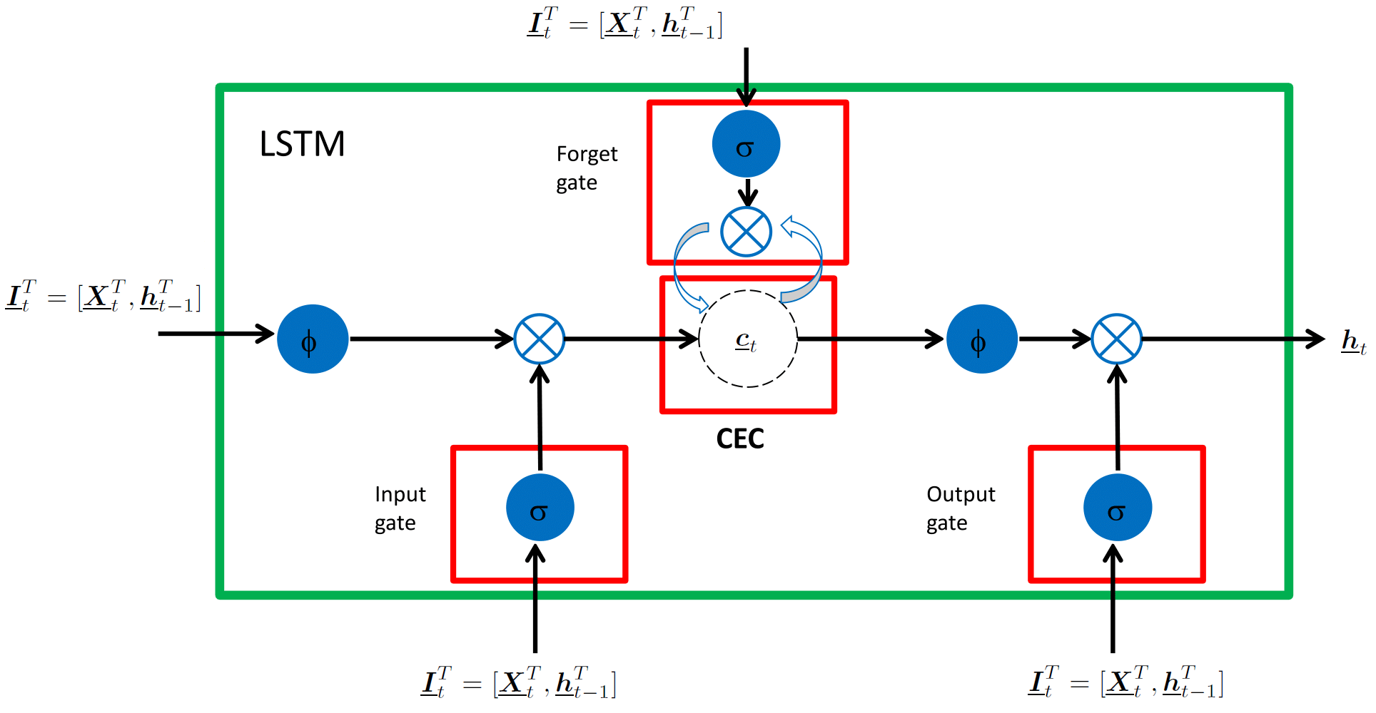
Figure 1: The diagram of a LSTM cell.

By following the work of Hochreiter et al. [5], we plot the diagram of the LSTM cell in Fig. 1. In this figure, $\phi$, $\sigma$ and $\otimes$ denote the hyperbolic tangent function, the sigmoid function (to be differed from the singular value operations denote as $\sigma_{\max}$ or $\sigma_{\min}$ with subscript) and the multiplication operation, respectively. All of them operate in an element-wise fashion. The LSTM cell has an input gate, an output gate, a forget gate and a constant error carousal (CEC) module. Mathematically, the LSTM cell can be written as

$$\underline{\boldsymbol{c}}_{t} = \sigma(\boldsymbol{W}_{f}\underline{\boldsymbol{I}}_{t})\underline{\boldsymbol{c}}_{t-1}+\sigma(\boldsymbol{W}_{i}\underline{\boldsymbol{I}}_{t})\phi(\boldsymbol{W}_{in}\underline{\boldsymbol{I}}_{t}),$$ (6)

$$\underline{\boldsymbol{h}}_{t} = \sigma(\boldsymbol{W}_{o}\underline{\boldsymbol{I}}_{t})\phi(\underline{\boldsymbol{c}}_{t}),$$ (7)

where $\underline{\boldsymbol{c}}_{t}\in\mathbb{R}^{N}$, column vector $\underline{\boldsymbol{I}}_{t}\in\mathbb{R}^{(M+N)}$ is a concatenation of the current input, $\underline{\boldsymbol{X}}_{t}\in\mathbb{R}^{M}$, and the previous output, $\underline{\boldsymbol{h}}_{t-1}\in\mathbb{R}^{N}$ (i.e., $\underline{\boldsymbol{I}}_{t}^{T}=[\underline{\boldsymbol{X}}_{t}^{T},\underline{\boldsymbol{h}}_{t-1}^{T}]$). Furthermore, $\boldsymbol{W}_{f}$, $\boldsymbol{W}_{i}$, $\boldsymbol{W}_{o}$ and $\boldsymbol{W}_{in}$ are weight matrices for the forget gate, the input gate, the output gate and the input, respectively.

Under the assumption $\underline{\boldsymbol{c}}_{0}=\underline{0}$, the hidden-state vector of the LSTM can be derived by induction as

$$\underline{\boldsymbol{c}}_{t}=\sum^{t}_{k=1}\underbrace{\bigg{[}\prod^{t}_{j=k+1}\sigma(\boldsymbol{W}_{f}\underline{\boldsymbol{I}}_{j})\bigg{]}}_{\text{forget gate}}\sigma(\boldsymbol{W}_{i}\underline{\boldsymbol{I}}_{k})\phi(\boldsymbol{W}_{in}\underline{\boldsymbol{I}}_{k}).$$ (8)

By setting $f(\cdot)$ in Eq. (2) to the hyperbolic-tangent function, we can compare outputs of the SRN and the LSTM below:

$$\underline{\boldsymbol{h}}_{t}^{SRN} = \phi\bigg{(}\sum^{t}_{k=1}\boldsymbol{W}_{c}^{t-k}\boldsymbol{W}_{in}\underline{\boldsymbol{X}}_{k}\bigg{)},$$ (9)

$$\underline{\boldsymbol{h}}_{t}^{LSTM} = \sigma(\boldsymbol{W}_{o}\underline{\boldsymbol{I}}_{t})\phi\bigg{(}\sum^{t}_{k=1}\underbrace{\bigg{[}\prod^{t}_{j=k+1}\sigma(\boldsymbol{W}_{f}\underline{\boldsymbol{I}}_{j})\bigg{]}}_{\text{forget gate}}\sigma(\boldsymbol{W}_{i}\underline{\boldsymbol{I}}_{k})\phi(\boldsymbol{W}_{in}\underline{\boldsymbol{I}}_{k})\bigg{)}.$$ (10)

We see from the above that $\boldsymbol{W}_{c}^{t-k}$ and $\prod^{t}_{j=k+1}\sigma(\boldsymbol{W}_{f}\underline{\boldsymbol{I}}_{j})$ play the same memory role for the SRN and the LSTM, respectively.

We can find many special cases where LSTM memory length exceeds SRN regardless of the choice of SRN’s model parameters ($\boldsymbol{W}_{c}$, $\boldsymbol{W}_{in}$). For example

$$\exists\boldsymbol{W}_{f}\quad s.t.\quad\min|\sigma(\boldsymbol{W}_{f}\underline{\boldsymbol{I}}_{j})|\geq\sigma_{\max}(\boldsymbol{W}_{c}),\quad\forall\sigma_{\max}(\boldsymbol{W}_{c})\in[0,1),$$

then

$$\Bigg{|}\prod^{t}_{j=k+1}\sigma(\boldsymbol{W}_{f}\underline{\boldsymbol{I}}_{j})\Bigg{|}\geq\sigma_{\max}(\boldsymbol{W}_{c})^{t-k},t\geq k.$$ (11)

As given in Eqs. (5) and (11), the impact of input $\underline{\boldsymbol{I}}_{k}$ on the output of the LSTM lasts longer than that of the SRN. This means there always exists a LSTM whose memory length is longer than SRN for all possible choices of SRN.

Conversely, to find a SRN with similar advantage to LSTM, we need to make sure $||\boldsymbol{W}_{c}^{t-k}||\geq 1\geq\Bigg{|}\prod^{t}_{j=k+1}\sigma(\boldsymbol{W}_{f}\underline{\boldsymbol{I}}_{j})\Bigg{|}$. Although such $\boldsymbol{W}_{c}$ exists, this condition would easily leads to memory explosion. For example, one close lower bound for $||\boldsymbol{W}_{c}^{t-k}||$ is $\sigma_{\min}(\boldsymbol{W}_{c})^{t-k}$, where $\sigma_{\min}(\boldsymbol{W}_{c})$ is the smallest singular value of $\boldsymbol{W}_{c}$ (this comes from the fact of $||\boldsymbol{AB}||\geq\sigma_{min}(\boldsymbol{A})||\boldsymbol{B}||$ and $||\boldsymbol{B}||=\sigma_{\max}(\boldsymbol{B})\geq\sigma_{min}(\boldsymbol{B})$, use induction for derivation). We need $\sigma_{\min}(\boldsymbol{W}_{c})\geq 1$, and since $||\boldsymbol{W}_{c}^{t-k}||\geq\sigma_{\min}(\boldsymbol{W}_{c})^{t-k}$, the SRN’s memory will grow exponentially and end up in memory explosion. Such memory explosion constraint does not exist in LSTM.

2.3 Memory of GRU

The GRU was originally proposed for neural machine translation [6]. It provides an effective alternative for the LSTM. Its operations can be expressed by the following four equations:

$$\underline{\boldsymbol{z}}_{t} = \sigma(\boldsymbol{W}_{z}\underline{\boldsymbol{X}}_{t}+\boldsymbol{U}_{z}\underline{\boldsymbol{h}}_{t-1}),$$ (12)

$$\underline{\boldsymbol{r}}_{t} = \sigma(\boldsymbol{W}_{r}\underline{\boldsymbol{X}}_{t}+\boldsymbol{U}_{r}\underline{\boldsymbol{h}}_{t-1}),$$ (13)

$$\underline{\boldsymbol{\tilde{h}}}_{t} = \phi(\boldsymbol{W}\underline{\boldsymbol{X}}_{t}+\boldsymbol{U}(\underline{\boldsymbol{r}}_{t}\otimes\underline{\boldsymbol{h}}_{t-1})),$$ (14)

$$\underline{\boldsymbol{h}}_{t} = \underline{\boldsymbol{z}}_{t}\underline{\boldsymbol{h}}_{t-1}+(\underline{\boldsymbol{1}}-\underline{\boldsymbol{z}}_{t})\underline{\boldsymbol{\tilde{h}}}_{t},$$ (15)

where $\underline{\boldsymbol{X}}_{t}$, $\underline{\boldsymbol{h}}_{t}$, $\underline{\boldsymbol{z}}_{t}$ and $\underline{\boldsymbol{r}}_{t}$ denote the input, the hidden-state, the update gate and the reset gate vectors, respectively, and $\boldsymbol{W}_{z}$, $\boldsymbol{W}_{r}$, $\boldsymbol{W}$, are trainable weight matrices. Its hidden-state is also its output, which is given in Eq. (15). Its diagram is shown in Fig. 2, where Concat denotes the vector concatenation operation.

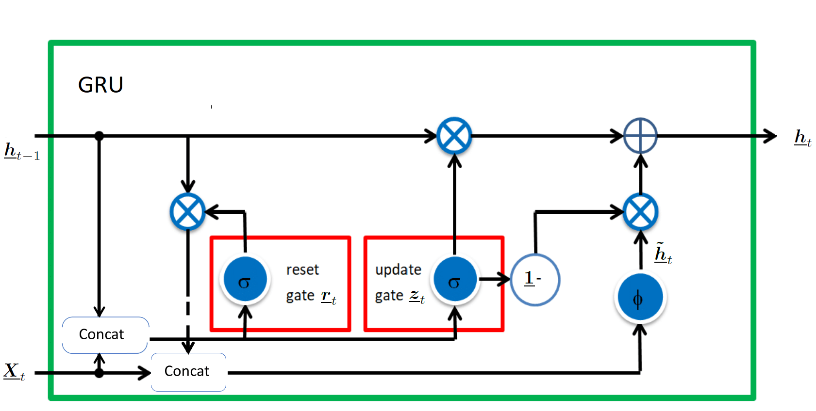
Figure 2: The diagram of a GRU cell.

By setting $\boldsymbol{U}_{z}$, $\boldsymbol{U}_{r}$ and $\boldsymbol{U}$ to zero matrices, we can obtain the following simplified GRU system:

$$\underline{\boldsymbol{z}}_{t} = \sigma(\boldsymbol{W}_{z}\underline{\boldsymbol{X}}_{t}),$$ (16)

$$\underline{\boldsymbol{\tilde{h}}}_{t} = \phi(\boldsymbol{W}\underline{\boldsymbol{X}}_{t}),$$ (17)

$$\underline{\boldsymbol{h}}_{t} = \underline{\boldsymbol{z}}_{t}\underline{\boldsymbol{h}}_{t-1}+(\underline{\boldsymbol{1}}-\underline{\boldsymbol{z}}_{t})\underline{\boldsymbol{\tilde{h}}}_{t}.$$ (18)

For the simplified GRU with the initial rest condition, we can derive the following by induction:

$$\underline{\boldsymbol{h}}_{t}=\sum^{t}_{k=1}\bigg{[}\underbrace{\prod^{t}_{j=k+1}\sigma(\boldsymbol{W}_{z}\underline{\boldsymbol{X}}_{j})}_{\text{update gate}}\bigg{]}(\underline{\boldsymbol{1}}-\sigma(\boldsymbol{W}_{z}\underline{\boldsymbol{X}}_{k}))\phi(\boldsymbol{W}\underline{\boldsymbol{X}}_{k}).$$ (19)

By comparing Eqs. (8) and (19), we see that the update gate of the simplified GRU and the forget gate of the LSTM play the same role. In other words, there is no fundamental difference between GRU and LSTM. Such finding is substantiated by the non-conclusive performance comparison between GRU and LSTM conducted in [15, 16, 17].

Because of the presence of the multiplication term introduced by the forget gate and the update gate in Eqs. (8) and (19), the longer the distance of $t-k$, the smaller these terms. Thus, the memory responses of LSTM and GRU to $I_{k}$ diminish inevitably as $t-k$ becomes larger. This phenomenon occurs regardless of the choice of model parameters. For complex language tasks that require long memory responses such as sentence parsing, LSTM’s and GRU’s memory decay may have significant impacts to their performance.

3 Extended Long Short-Term Memory (ELSTM)

To address this design limitation, we introduce a scaling factor to compensate the fast decay of the input response. This leads to a new solution called the extended LSTM (ELSTM). The ELSTM cell is depicted in Fig. 3, where $\underline{\boldsymbol{s}}_{i}\in\mathbb{R}^{N}$, $i=1,\cdots,t-1$ is the trainable input scaling vectors

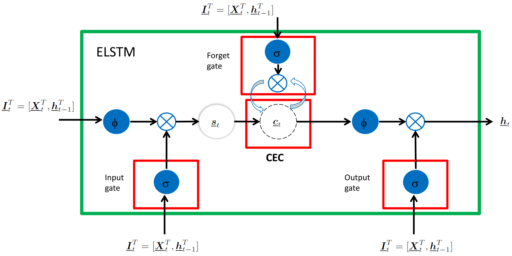
Figure 3: The diagrams of the ELSTM cell.

The ELSTM cell can be described by

$$\underline{\boldsymbol{c}}_{t} = \sigma(\boldsymbol{W}_{f}\underline{\boldsymbol{I}}_{t})\underline{\boldsymbol{c}}_{t-1}+\underline{\boldsymbol{s}}_{t}\sigma(\boldsymbol{W}_{i}\underline{\boldsymbol{I}}_{t})\phi(\boldsymbol{W}_{in}\underline{\boldsymbol{I}}_{t}),$$ (20)

$$\underline{\boldsymbol{h}}_{t} = \sigma(\boldsymbol{W}_{o}\underline{\boldsymbol{I}}_{t})\phi(\underline{\boldsymbol{c}}_{t}).$$ (21)

a bias term $\underline{\boldsymbol{b}}\in\mathbb{R}^{N}$ for $\underline{\boldsymbol{c}}_{t}$ is omitted in Equation 21. As shown above, we introduce scaling factor, $\underline{\boldsymbol{s}}_{i}$, $i=1,\cdots,t-1$, to the ELSTM to increase or decrease the impact of input $\underline{\boldsymbol{I}}_{i}$ in the sequence.

To show that the ELSTM has longer memory than the LSTM, we first derive a closed form expression of $\underline{\boldsymbol{h}}_{t}$ as

$$\underline{\boldsymbol{h}}_{t}=\sigma(\boldsymbol{W}_{o}\underline{\boldsymbol{I}}_{t})\phi\bigg{(}\sum^{t}_{k=1}\underline{\boldsymbol{s}}_{k}\bigg{[}\prod^{t}_{j=k+1}\sigma(\boldsymbol{W}_{f}\underline{\boldsymbol{I}}_{j})\bigg{]}\sigma(\boldsymbol{W}_{i}\underline{\boldsymbol{I}}_{k})\phi(\boldsymbol{W}_{in}\underline{\boldsymbol{I}}_{k})\bigg{)}.$$ (22)

Then, we can find the following special case:

$$\exists\underline{\boldsymbol{s}}_{k}\quad s.t.\quad\Bigg{|}\underline{\boldsymbol{s}}_{k}\prod^{t}_{j=k+1}\sigma(\boldsymbol{W}_{f}\underline{\boldsymbol{I}}_{j})\Bigg{|}\geq\Bigg{|}\prod^{t}_{j=k+1}\sigma(\boldsymbol{W}_{f}\underline{\boldsymbol{I}}_{j})\Bigg{|}\quad\forall\boldsymbol{W}_{f}.$$ (23)

By comparing Eq. (23) with Eq. (11), we conclude that there always exists an ELSTM whose memory is longer than LSTM for all choices of LSTM. Conversely, we cannot find such LSTM with similar advantage to ELSTM. This demonstrates the ELSTM’s system advantage by design to LSTM. Such a scalar-based solution can also be found in work for convolutional neural networks (CNN) [18].

The numbers of parameters used by various RNN cells are compared in Table 1, where $\underline{\boldsymbol{X}}_{t}\in\mathbb{R}^{M}$, $\underline{\boldsymbol{h}}_{t}\in\mathbb{R}^{N}$ and $t=1,\cdots,T$. As shown in Table 1, the number of parameters of the ELSTM cell depends on the maximum length, $T$, of the input sequences, which makes the model size uncontrollable. To address this problem, we choose a fixed $T_{s}$ (with $T_{s}<T$) as the upper bound on the number of scaling factors, and set $\underline{\boldsymbol{s}}_{k}=\underline{\boldsymbol{s}}_{(k-1)\mbox{ mod }T_{s}+1}$, if $k>T_{s}$ and $k$ starts from 1, where mod denotes the modulo operator. In other words, the sequence of scaling factors is a periodic one with period $T_{s}$, so the elements in a sequence that are distanced by the length of $T_{s}$ will share the same scaling factor.

Table 1: Comparison of Parameter Numbers.

Cell	Number of Parameters
LSTM	$4N(M+N+1)$
GRU	$3N(M+N+1)$
ELSTM	$4N(M+N+1)+N(T+1)$

The ELSTM cell with periodic scaling factors can be described by

$$\underline{\boldsymbol{c}}_{t} = \sigma(\boldsymbol{W}_{f}\underline{\boldsymbol{I}}_{t})\underline{\boldsymbol{c}}_{t-1}+\underline{\boldsymbol{s}}_{t_{s}}\sigma(\boldsymbol{W}_{i}\underline{\boldsymbol{I}}_{t})\phi(\boldsymbol{W}_{in}\underline{\boldsymbol{I}}_{t}),$$ (24)

$$\underline{\boldsymbol{h}}_{t} = \sigma(\boldsymbol{W}_{o}\underline{\boldsymbol{I}}_{t})\phi(\underline{\boldsymbol{c}}_{t}),$$ (25)

where $t_{s}=(t-1)\mbox{ mod }T_{s}+1$. We observe that the choice of $T_{s}$ affects the network performance. Generally speaking, a small $T_{s}$ value is suitable for simple language tasks that demand shorter memory while a larger $T_{s}$ value is desired for complex ones that demand longer memory. For the particular sequence-to-sequence (seq2seq [8, 9]) RNN models, a larger $T_{s}$ value is always preferred. We will elaborate the parameter settings in Sec. 5.

3.1 Study of Scaling Factor

To examine the memory capability of the scaling factor, we carry out the following experiment. The RNN cell is asked to tell whether a special element “A” exists in the sequence of a single “A” and multiple “B”s of length $T$. The training data contains $T$ number of positive samples where “A” locates from position 1 to $T$, and 1 negative sample where there is no “A” exists. The cell takes in the whole sequence and generates the output at time step $T$ as shown in Fig. 4.

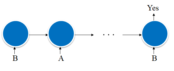
Figure 4: Experiment of estimating the presence of “A”.

We would like to see the memory response of LSTM and ELSTM to “A”. If “A” lies at the beginning of the sequence, the LSTM’s memory decay may cause it lose the information of “A”’s presence. The memory responses of LSTM and ELSTM to the input $\underline{\boldsymbol{I}}_{k}$ are calculated as:

$$\underline{\boldsymbol{mr}}^{LSTM}_{k} = \bigg{[}\prod^{T}_{j=k+1}\sigma(\boldsymbol{W}_{f}\underline{\boldsymbol{I}}_{j})\bigg{]}\sigma(\boldsymbol{W}_{i}\underline{\boldsymbol{I}}_{k})\phi(\boldsymbol{W}_{in}\underline{\boldsymbol{I}}_{k}),$$ (26)

$$\underline{\boldsymbol{mr}}^{ELSTM}_{k} = \underline{\boldsymbol{s}}_{k}\bigg{[}\prod^{T}_{j=k+1}\sigma(\boldsymbol{W}_{f}\underline{\boldsymbol{I}}_{j})\bigg{]}\sigma(\boldsymbol{W}_{i}\underline{\boldsymbol{I}}_{k})\phi(\boldsymbol{W}_{in}\underline{\boldsymbol{I}}_{k}),$$ (27)

The detailed model settings can be found in Table. 2

Table 2: Network parameters for the toy experiment.

Number of RNN layers	1
Embedding layer vector size	2
Number of RNN cells	1
Batch size	5

We carry out multiple such experiments by increase the sample length $T$ by 1 at a time and see when LSTM cannot keep up with ELSTM. We train the LSTM and ELSTM models with equal number of epochs until both report no further change of training loss.

We found when $T=60$, LSTM’s training loss starts to plateau while ELSTM can further decrease to zero. As a result, LSTM starts to “forget” when $T>=60$. The detailed plot of the memory responses for two particular samples are shown in Fig. 5

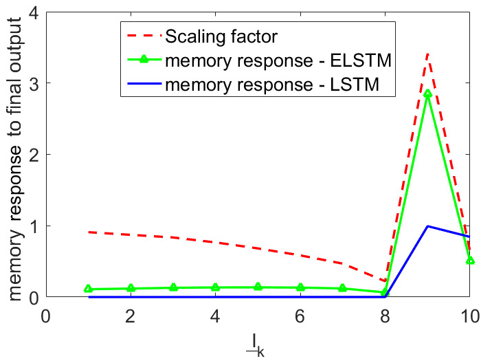
(a)

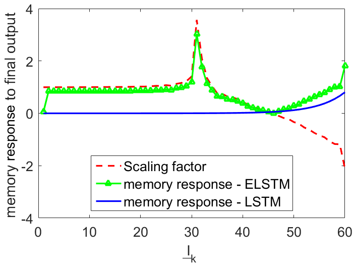
(b)

Figure 5: Comparison of memory response between LSTM and ELSTM.

Fig. 5a shows the memory response of trained LSTM and ELSTM on a sample with $T=10$ with “A” at position 9. It can be seen that although both LSTM and ELSTM have stronger memory response at “A”, the ELSTM attends better than LSTM since its response at position 10 is smaller than LSTM’s. We can also find that the scaling factor has larger value at the beginning and then slowly decreases as the location comes closer to the end. It then spikes at position 9. We can imagine that the scaling factor is doing its compensating job at both ends of the sequence.

Fig. 5b shows the memory response of trained LSTM and ELSTM on a sample with $T=60$ with “A” at location 30. In this case, the LSTM is not able to “remember” the presence of “A” and it does not have strong response to it. The scaling factor is doing its compensating job at the first half the sequence and especially in the middle and this causes strong ELSTM’s response to “A”.

Even though scaling factor cannot adaptively change its value once it is trained, it is able to learn the pattern of model’s rate of memory decay and the averaged importance of that position in the training set.

It is important to point out that the scaling factor needs to be initialized to 1 for each cell.

4 Dependent BRNN (DBRNN) Model

A single RNN cell is rarely used in practice due to its limited capability in modeling real-world problems. To build a more powerful RNN model, it is often to integrate several cells with different probabilistic models. To give an example, the sequence-to-sequence problem demands an RNN model to predict an output sequence, $\{\underline{\boldsymbol{Y}}_{t}\}^{T^{\prime}}_{t=1}$ with $\underline{\boldsymbol{Y}}_{i}\in\mathbb{R}^{N}$, based on an input sequence, $\{\underline{\boldsymbol{X}}_{t}\}^{T}_{t=1}$ with $\underline{\boldsymbol{X}}_{i}\in\mathbb{R}^{M}$, where $T$ and $T^{\prime}$ are lengths of the input and the output sequences, respectively. To solve this problem, we propose a macro RNN model, called the dependent BRNN (DBRNN), in this section. Our design is inspired by pros and cons of two RNN models; namely, the bidirectional RNN (BRNN) [7] and the encoder-decoder design [6]. We will review the BRNN and the encoder-decoder in Sec. 4.1. Then, the DBRNN is proposed in Sec. 4.2.

4.1 BRNN and Encoder-Decoder

As its name indicates, BRNN takes inputs in both forward and backward directions as shown in Fig. 6, and it has two RNN cells to take in the input: one takes the input in the forward direction, the other takes the input in the backward direction.

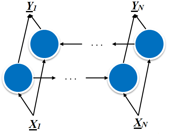
Figure 6: The diagram of BRNN.

The motivation for BRNN is to fully utilize the input sequence if future information ($\{\underline{\boldsymbol{X}}_{i}\}^{T}_{i=t+1}$) is accessible. This is especially helpful if current output $\underline{\boldsymbol{Y}}_{t}$ is also a function of future inputs. The conditional probability density function of BRNN is in form of

$$\underline{\boldsymbol{p}}_{t} = P(\underline{\boldsymbol{Y}}_{t}|\{\underline{\boldsymbol{X}}_{i}\}^{T}_{i=1})=\boldsymbol{W}^{f}\underline{\boldsymbol{p}}^{f}_{t}+\boldsymbol{W}^{b}\underline{\boldsymbol{p}}^{b}_{t},$$ (28)

$$\underline{\boldsymbol{\hat{Y}}}_{t} = \operatorname*{argmax}_{\underline{\boldsymbol{Y}}_{t}}\underline{\boldsymbol{p}}_{t},$$ (29)

where

$$\underline{\boldsymbol{p}}^{f}_{t} = P(\underline{\boldsymbol{Y}}_{t}|\{\underline{\boldsymbol{X}}_{i}\}^{t}_{i=1}),$$ (30)

$$\underline{\boldsymbol{p}}^{b}_{t} = P(\underline{\boldsymbol{Y}}_{t}|\{\underline{\boldsymbol{X}}_{i}\}^{T}_{i=t}),$$ (31)

and $\boldsymbol{W}^{f}$ and $\boldsymbol{W}^{b}$ are trainable weights, $\underline{\boldsymbol{\hat{Y}}}_{t}$ is the predicted output element at time step $t$. So the output is a combination of the density estimation of a forward RNN and the output of a backward RNN. Due to the bidirectional design, the BRNN can utilize the information of the entire input sequence to predict each individual output element. One example where such treatment is helpful is generating a sentence like “this is an apple” for language modeling (predicts the next word given proceeding words in a sentence). In this case, the word “an” strongly associates with its following word “apple”, in a forward directional RNN model, it would find difficulty in generating “an” before “apple”.

Encoder-decoder was first proposed for machine translation (MT) along with GRU in [6]. It was motivated to handle the situation when $T^{\prime}\neq T$. It has two RNN cells: an encoder and a decoder. The detailed design of one of the early proposals [8] of encoder-decoder RNN model is illustrated in Fig. 7.

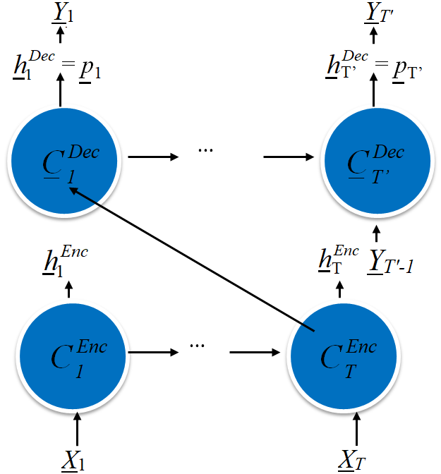
Figure 7: The diagram of sequence to sequence (seq2seq).

As can be seen in Fig. 7, the encoder (denoted by Enc) takes the input sequence of length $T$ and generates its output $\underline{\boldsymbol{h}}^{\text{Enc}}_{i}$ and hidden state $\underline{\boldsymbol{c}}^{\text{Enc}}_{i}$, where $i\in\{1,...,T\}$. In seq2seq model, the encoder’s hidden state at time step $T$ is used as the representation of the input sequence. The decoder then utilizes the hidden state information to generate the output sequence of length $T^{\prime}$ by initializing its hidden state $\underline{\boldsymbol{c}}^{Dec}_{1}$ as $\underline{\boldsymbol{c}}^{Enc}_{T}$. So the decoding process starts after the encoder has processed the entire input sequence. In practice, the input to the decoder at time step 1 is a pre-defined start decoding symbol. At the following time steps, the previous output $\underline{\boldsymbol{Y}}_{t-1}$ will be used as input. The decoder will stop the decoding process if a special pre-defined stopping symbol is generated.

As compare with BRNN, the encoder-decoder is not only advantageous in its ability in handling input/output sequences of different length but also capable in generating better aligned output sequences by explicitly feeding previous predicted outputs back to its decoder. Thus, the encoder-decoder estimates the following density function

$$\underline{\boldsymbol{p}}_{t} = P(\underline{\boldsymbol{Y}}_{t}|\{\underline{\boldsymbol{\hat{Y}}}_{i}\}^{t-1}_{i=1},\{\underline{\boldsymbol{X}}_{i}\}^{T}_{i=1})$$ (32)

$$\underline{\boldsymbol{\hat{Y}}}_{t} = \operatorname*{argmax}_{\underline{\boldsymbol{Y}}_{t}}\underline{\boldsymbol{p}}_{t}\quad\forall t\in\{1,...,T^{\prime}\}.$$ (33)

For better encoder-decoder aliment, various attention mechanism has been proposed for encoder-decoder model. In [9, 10], additional weighted connections are introduced to connect the decoder to the hidden state of the encoder.

On the other hand, the encoder-decoder system is vulnerable to previous erroneous predictions in the forward path. Recently, the BRNN was introduced to the encoder by Bahdanau et al. [10], yet their design does not address the erroneous prediction problem.

4.2 DBRNN Model and Training

Being motivated by the observations in Sec. 4.1, we propose a multi-task BRNN model, called the dependent BRNN (DBRNN), to achieve the following objectives:

$$\underline{\boldsymbol{p}}_{t} = \boldsymbol{W}^{f}\underline{\boldsymbol{p}}_{t}^{f}+\boldsymbol{W}^{b}\underline{\boldsymbol{p}}_{t}^{b}$$ (34)

$$\underline{\boldsymbol{\hat{Y}}}^{f}_{t} = \operatorname*{argmax}_{\underline{\boldsymbol{Y}}_{t}}\underline{\boldsymbol{p}}_{t}^{f},$$ (35)

$$\underline{\boldsymbol{\hat{Y}}}^{b}_{t} = \operatorname*{argmax}_{\underline{\boldsymbol{Y}}_{t}}\underline{\boldsymbol{p}}_{t}^{b},$$ (36)

$$\underline{\boldsymbol{\hat{Y}}}_{t} = \operatorname*{argmax}_{\underline{\boldsymbol{Y}}_{t}}\underline{\boldsymbol{p}}_{t}$$ (37)

where

$$\underline{\boldsymbol{p}}_{t}^{f} = P(\underline{\boldsymbol{Y}}_{t}|\{\underline{\boldsymbol{X}}_{i}\}^{T}_{i=1},\{\underline{\boldsymbol{\hat{Y}}}^{f}_{i}\}^{t-1}_{i=1}),$$ (38)

$$\underline{\boldsymbol{p}}_{t}^{b} = P(\underline{\boldsymbol{Y}}_{t}|\{\underline{\boldsymbol{X}}_{i}\}^{T}_{i=1},\{\underline{\boldsymbol{\hat{Y}}}^{b}_{i}\}^{T^{\prime}}_{i=t+1}),$$ (39)

$$\underline{\boldsymbol{p}}_{t} = P(\underline{\boldsymbol{Y}}_{t}|\{\underline{\boldsymbol{X}}_{i}\}^{T}_{i=1}),$$ (40)

and $\boldsymbol{W}^{f}$ and $\boldsymbol{W}^{b}$ are trainable weights. As shown in Eqs. (35), (36) and (37), the DBRNN has three learning objectives: 1) the target sequence for the forward RNN prediction, 2) the reversed target sequence for the backward RNN prediction, and 3) the target sequence for the bidirectional prediction.

The DBRNN model is shown in Fig. 8. It consists of a lower and an upper BRNN branches. At each time step, the input to the forward and the backward parts of the upper BRNN is the concatenated forward and backward outputs from the lower BRNN branch. The final bidirectional prediction is the pooling of both the forward and the backward predictions. We will show later that this design will make the DBRNN robust to previous erroneous predictions.

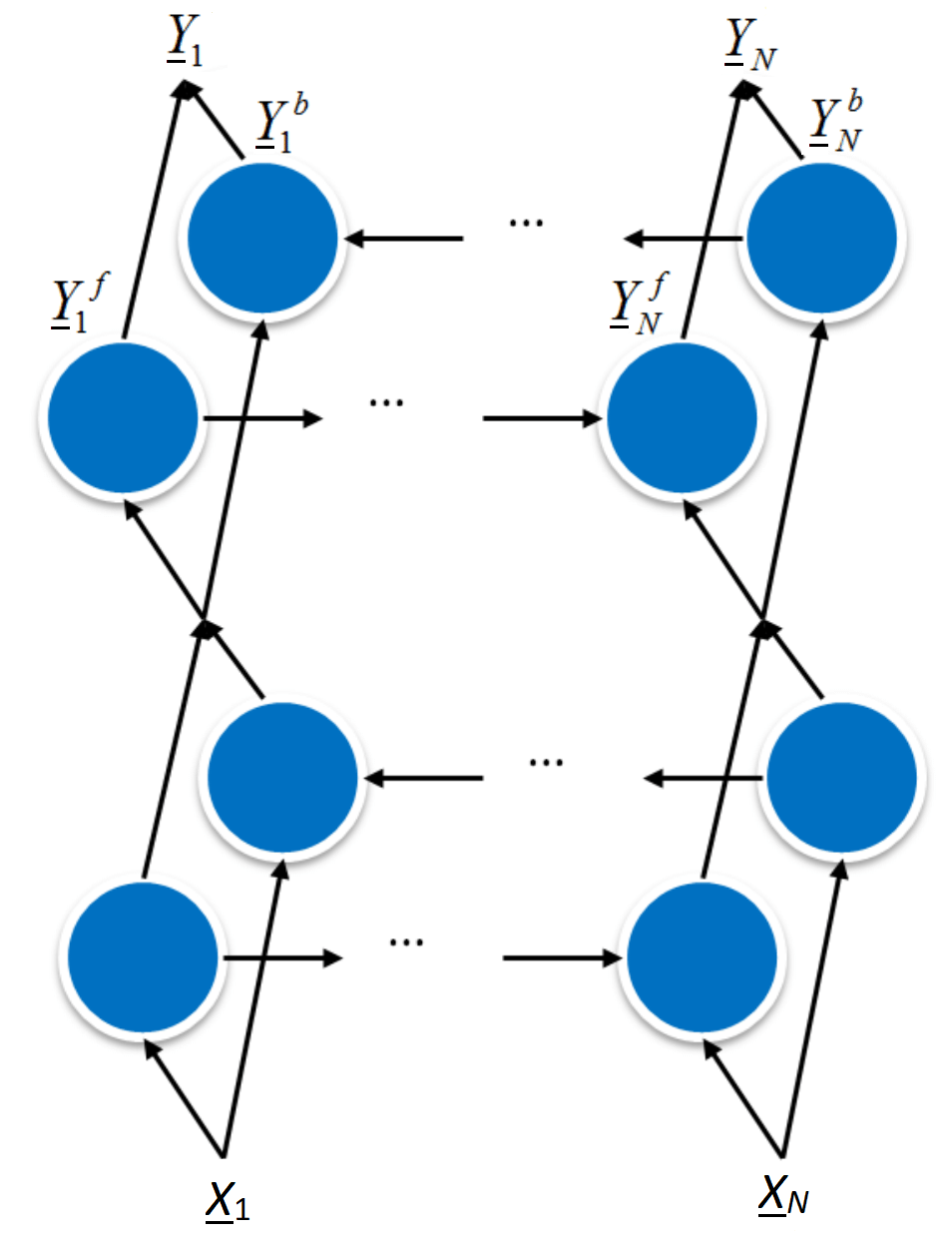
Figure 8: The DBRNN model.

Let $F(\cdot)$ be the cell function. The input is fed into the forward and backward RNN of the lower BRNN branch as

$$\underline{\boldsymbol{h}}_{t}^{f}=F_{l}^{f}\Big{(}\underline{\boldsymbol{x}}_{t},\underline{\boldsymbol{c}}_{l(t-1)}^{f}\Big{)},\quad\underline{\boldsymbol{h}}_{t}^{b}=F_{l}^{b}\Big{(}\underline{\boldsymbol{x}}_{t},\underline{\boldsymbol{c}}_{l(t+1)}^{b}\Big{)},\quad\underline{\boldsymbol{h}}_{t}=\begin{bmatrix}\underline{\boldsymbol{h}}_{t}^{f}\\ \underline{\boldsymbol{h}}_{t}^{b}\end{bmatrix},$$ (41)

where $\underline{\boldsymbol{c}}$ and $l$ denote the cell hidden state and the lower BRNN, respectively. The final output, $\underline{\boldsymbol{h}}_{t}$, of the lower BRNN is the concatenation of the output, $\underline{\boldsymbol{h}}_{t}^{f}$, of the forward RNN and the output, $\underline{\boldsymbol{h}}_{t}^{b}$, of the backward RNN. Similarly, the upper BRNN generates the final output $\underline{\boldsymbol{p}}_{t}$ as

$$\underline{\boldsymbol{p}}_{t}^{f}=F_{u}^{f}\Big{(}\underline{\boldsymbol{h}}_{t},\underline{\boldsymbol{c}}_{u(t-1)}^{f}\Big{)},\quad\underline{\boldsymbol{p}}_{t}^{b}=F_{u}^{b}\Big{(}\underline{\boldsymbol{h}}_{t},\underline{\boldsymbol{c}}_{u(t+1)}^{b}\Big{)},\quad\underline{\boldsymbol{p}}_{t}=\boldsymbol{W}^{f}\underline{\boldsymbol{p}}_{t}^{f}+\boldsymbol{W}^{b}\underline{\boldsymbol{p}}_{t}^{b},$$ (42)

where $u$ denotes the upper BRNN. To generate forward prediction $\underline{\boldsymbol{\hat{Y}}}^{f}_{t}$ and backward prediction $\underline{\boldsymbol{\hat{Y}}}^{b}_{t}$, the forward and backward paths of the upper BRNN branch are separately trained by the original and the reversed target sequences, respectively. The results of forward and backward predictions of the upper RNN branch are then combined to generate the final result.

There are three errors: 1) forward prediction error $e_{f}$ for $\underline{\boldsymbol{\hat{Y}}}^{f}_{t}$, 2) backward prediction error $e_{b}$ for $\underline{\boldsymbol{\hat{Y}}}^{b}_{t}$, and 3) bidirectional prediction error $e$ for $\underline{\boldsymbol{\hat{Y}}}_{t}$ . To train the proposed DBRNN, $e_{f}$ is backpropagated through time to the upper forward RNN and the lower BRNN, $e_{b}$ is backpropagated through time to the upper backward RNN and the lower BRNN, and $e$ is backpropagated through time to the entire model.

As it can been seen that DBRNN being an encoder-decoder can better handle output alignment. By introducing the bidirectional design to its decoder, DBRNN is also better than encoder-decoder in handling previous erroneous predictions. To show that DBRNN is more robust to previous erroneous predictions than one-directional models, we compare their cross entropy defined as

$$l=-\sum^{K}_{k=1}p_{t,k}\text{log}(\hat{p}_{t,k}),$$ (43)

where $K$ is the total number of classes (e.g. the size of vocabulary for the language task), $\hat{p}_{t}$ is the predicted distribution, and $p_{t}$ is the ground truth distribution with $k^{\prime}$ as the ground truth label. It is in form of one-hot vector. That is,

$$\underline{\boldsymbol{p}}_{t}=(\delta_{1,k^{\prime}},\cdots,\delta_{k^{\prime},k^{\prime}},\cdots,\delta_{K,k^{\prime}})^{T},\quad k=1,\cdots,K,$$

where $\delta_{k,k^{\prime}}$ is the Kronecker delta function. Based on Eq. (34), $l$ can be further expressed as

$$l = -\sum^{K}_{k=1}p_{t,k}\text{log}(W^{f}_{k}\hat{p}^{f}_{t,k}+W^{b}_{k}\hat{p}^{b}_{t,k}),$$ (44)

$$= -\text{log}(W^{f}_{k^{\prime}}\hat{p}^{f}_{t,k^{\prime}}+W^{b}_{k^{\prime}}\hat{p}^{b}_{t,k^{\prime}}).$$ (45)

We can select $W^{f}_{k^{\prime}}$ and $W^{b}_{k^{\prime}}$ such that $W^{f}_{k^{\prime}}\hat{p}^{f}_{t,k^{\prime}}+W^{b}_{k^{\prime}}\hat{p}^{b}_{t,k^{\prime}}$ is greater than $\hat{p}^{f}_{t,k^{\prime}}$ and $\hat{p}^{b}_{t,k^{\prime}}$. Then, we obtain

$$l < -\sum^{K}_{k=1}\text{log}(\hat{p}^{f}_{tk}),$$ (46)

$$l < -\sum^{K}_{k=1}\text{log}(\hat{p}^{b}_{tk}).$$ (47)

The above two equations indicate that there always exists a DBRNN with better performance as compared to encoder-decoder regardless of which parameters the encoder-decoder chose. So DBRNN does not have the encoder-decoder’s model limitations.

It is worthwhile to compare the proposed DBRNN and the bi-attention model in Cheng et al. [1]. Both of them have bidirectional predictions for the output, yet there are three main differences. First, the DBRNN provides a generic solution to the SISO problem without being restricted to dependency parsing. The target sequences in training (namely, $\underline{\boldsymbol{\hat{Y}}}^{f}_{t}$, $\underline{\boldsymbol{\hat{Y}}}^{b}_{t}$ and $\underline{\boldsymbol{\hat{Y}}}_{t}$) are the same for the DBRNN while the solution in [1] has different target sequences. Second, the attention mechanism is used in [1] but not in the DBRNN.

5 Experiments

5.1 Experimental Setup

In the experiments, we compare the performance of five RNN macro-models:

1. basic one-directional RNN (basic RNN);

2. bidirectional RNN (BRNN);

3. sequence-to-sequence (seq2seq) RNN [8] (a variant of the encoder-decoder);

4. seq2seq with attention [9];

5. dependent bidirectional RNN (DBRNN), which is proposed in this work.

For each RNN model, we compare three cell designs: LSTM, GRU, and ELSTM.

We conduct experiments on three problems: part of speech (POS) tagging, language modeling and dependency parsing (DP). We report the testing accuracy for the POS tagging problem, the perplexity (i.e. the natural exponential of the model’s cross-entropy loss) for LM and the unlabeled attachment score (UAS) and the labeled attachment score (LAS) for the DP problem. The POS tagging task is an easy one which requires shorter memory while the LM and DP task demand longer memory. For the latter two tasks, there exist more complex relations between the input and the output. For the DP problem, we compare our solution with the GRU-based bi-attention model (bi-Att). Furthermore, we compare the DBRNN using the ELSTM cell with two other non-RNN-based neural network methods. One is transition-based DP with neural network (TDP) proposed by Chen et al. [19]. The other is convolutional seq2seq (ConvSeq2seq) proposed by Gehring et al. [2]. For the proposed DBRNN, we show the result for the final combined output (namely, $p_{t}$). We adopt $T_{s}=1$ in the basic RNN, BRNN, and DBRNN models and $T_{s}=100$ in the other two seq2seq models for the POS tagging problem. We use $T_{s}=3$ and $T_{s}=100$ in all models for the LM problem and the DP problem, respectively.

The training, validation and testing dataset used for LM is from the Penn Treebank (PTB) [20]. The PTB has 42,068, 3,370 and 3,761 training, validation and testing sentences respectively. It has in total 10,000 tokens. The training dataset used for the POS tagging and DP problems are from the Universal Dependency 2.0 English branch (UD-English). It contains 12,543 sentences and 14,985 unique tokens. The test dataset in both experiments is from the test English branch (gold, en.conllu) of CoNLL 2017 shared task development and test data. The input to the POS tagging and the DP problems are the stemmed and lemmatized sequences (column 3 in CoNLL-U format). The target sequence for the POS tagging is the universal POS tag (column 4). The target sequence for the DP is the interleaved dependency relation to the headword (relation, column 8) and its headword position (column 7). As a result, the length of the target sequence for the DP is twice of the length of the input sequence.

Table 3: Training dataset.

	# Training	# Validation	# Testing	# Tokens
PTB	42,068	3,370	3,761	10,000
UD 2.0	12,543	2,002	2,077	14,985

Table 4: Network parameters and training details.

Parameter	POS & DP	LM
Embedding layer vector size	512	5
Number of RNN cells	512	5
Batch size	20	50
Number of RNN layers	1
Training steps	11 epochs
Learning rate	0.5
Optimizer	AdaGrad[21]

The input is first fed into a trainable embedding layer [22] before it is sent to the actual network. Table 4 shows the detailed network and training specifications. We do not finetune network hyper-parameters or apply any engineering trick (e.g. feeding additional inputs other than the raw embedded input sequences) for the best possible performance since our main goal is to compare the performance of the LSTM, GRU, ELSTM cells under various macro-models.

Table 5: LM test perplexity

	LSTM	GRU	ELSTM
BASIC RNN	267.47	262.39	248.60
BRNN	78.56	82.83	71.65
Seq2seq	296.92	293.99	266.98
Seq2seq with Att	17.86	232.20	11.43
DBRNN	9.80	24.10	6.18

Table 6: DP test results (UAS/LAS %)

	LSTM	GRU	ELSTM
BASIC RNN	43.24/25.28	45.24/29.92	58.49/36.10
BRNN	37.88/25.26	16.86/8.95	55.97/35.13
Seq2seq	29.38/6.05	36.47/13.44	48.58/24.05
Seq2seq with Att	31.82/16.16	43.63/33.98	64.30/52.60
DBRNN	51.38/39.71	52.23/37.25	61.35/43.32
Bi-Att [1]		59.97/44.94

Table 7: POS tagging test accuracy (%)

	LSTM	GRU	ELSTM
BASIC RNN	87.30	87.51	87.44
BRNN	89.55	89.39	89.29
Seq2seq	24.43	35.27	50.42
Seq2seq with Att	31.34	34.60	81.72
DBRNN	89.86	89.06	89.28

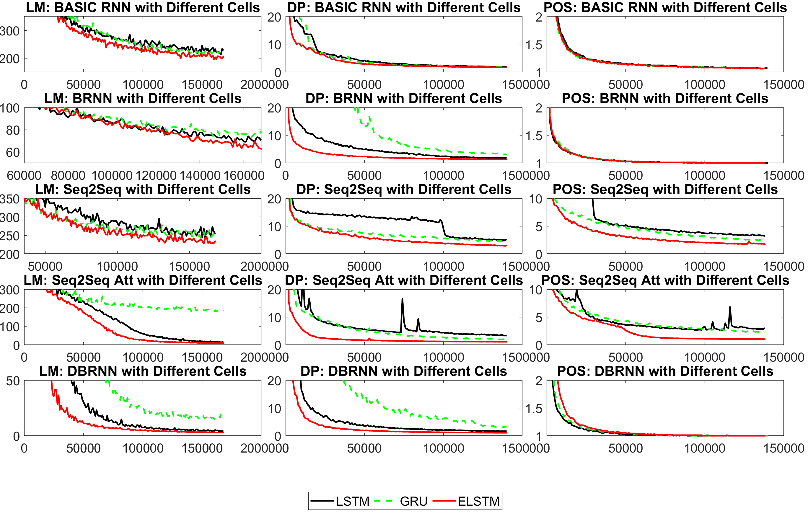
Figure 9: The training perplexity vs. training steps of different cells.

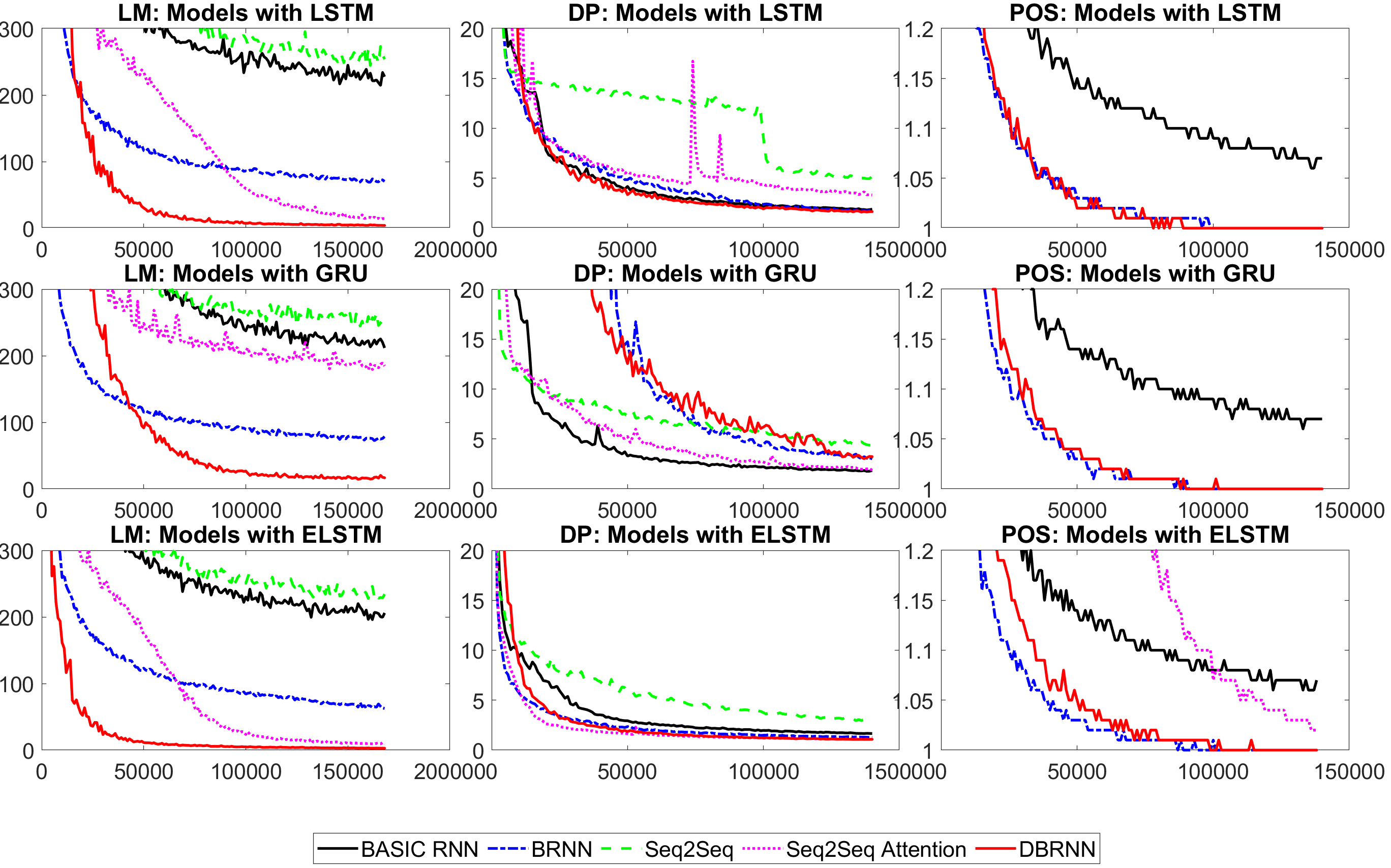
Figure 10: The training perplexity vs. training steps of different macro models.

5.2 Comparison of RNN Models

The results of the LM, the DP and the POS tagging are shown in Tables 5 - 6, respectively.

The training perplexity of different cell models and the macro models are shown in Fig. 9 and 10 respectively. We see that the proposed ELSTM cell outperforms the LSTM and GRU cells in most RNN models. This is especially true for complex language tasks like LM and DP, where the ELSTM cell outperforms other cell designs by a significant margin. The ELSTM cell even outperforms the bi-Att model, which was designed specifically for the DP task. This demonstrates the effectiveness of the sequence of scaling factors adopted by the ELSTM cell. It allows the network to retain longer memory with better attention. For the simple POS tagging task, ELSTM also shows equal or better performance in comparison to other cell models. Overall, ELSTM delivers good performance across tasks with different complexity.

The ELSTM cell with large $T_{s}$ value perform particularly well for the seq2seq (with and without attention) model. The hidden state, $c_{t}$, of ELSTM cell is more expressive in representing patterns over a longer distance. Since the seq2seq design relies on the expressive power of a hidden state, ELSTM has a clear advantage.

Generally speaking, the scaling factor number depends on the memory length required by the specific task. For example, the output of POS tagging task is mostly a function of its immediate before, current and after inputs. Thus, the observation of using only one scaling factor gave the optimal performance for POS tagging makes sense since the memory length required for this task is mostly 1. The same observation goes for the language modeling task, where the memory length required is widely believed to be 3-5 and the best performance was achieved when the scaling factor number is 3. On the other hand, the encoder-decoder RNN behaves differently, where the usage of more than the required scaling factor number tends to yield better performance. This may have something to do with the memory length required at the decoder side is not the same as the one for the encoder. The underlining mechanism demands future study. Our recommendation is to estimate the required memory length before hyperparameter selection. If the estimation is not possible or reliable, one can begin by setting the scaling factor number to the maximum training sequence length and searching for its optimal value by binary search.

For the DBRNN, we see that the it achieves the best performance across different macro models for the LM problem. It also outperforms the BRNN and the seq2seq in both the POS tagging and the DP problems regardless of the cell types. This shows its robustness. The DBRNN may overfit to the training data in other cases. One may use a proper regularization scheme in the training process to address it, which will be an interesting future work item.

To substantiate our claim in Sec. 2, we conduct additional experiments to show the robustness of the ELSTM cell and the DBRNN. Specifically, we compare the performance of the same five models with LSTM, and ELSTM with $I_{t}=X_{t}$ for the same language tasks. We do not include the GRU cell since it inherently demands $\underline{\boldsymbol{I}}_{t}^{T}=[\underline{\boldsymbol{X}}_{t}^{T},\underline{\boldsymbol{h}}_{t-1}^{T}]$. The convergence behaviors of $\underline{\boldsymbol{I}}_{t}=\underline{\boldsymbol{X}}_{t}$ and $\underline{\boldsymbol{I}}_{t}^{T}=[\underline{\boldsymbol{X}}_{t}^{T},\underline{\boldsymbol{h}}_{t-1}^{T}]$ with the LSTM, ELSTM cell for the DP problem are shown in Fig. 11. We see that the ELSTM does not behave much differently between $\underline{\boldsymbol{I}}_{t}=\underline{\boldsymbol{X}}_{t}$ and $\underline{\boldsymbol{I}}_{t}^{T}=[\underline{\boldsymbol{X}}_{t}^{T},\underline{\boldsymbol{h}}_{t-1}^{T}]$ while the LSTM does. This shows the effectiveness of the ELSTM design regardless of the input. More performance comparison will be provided in the Appendix.

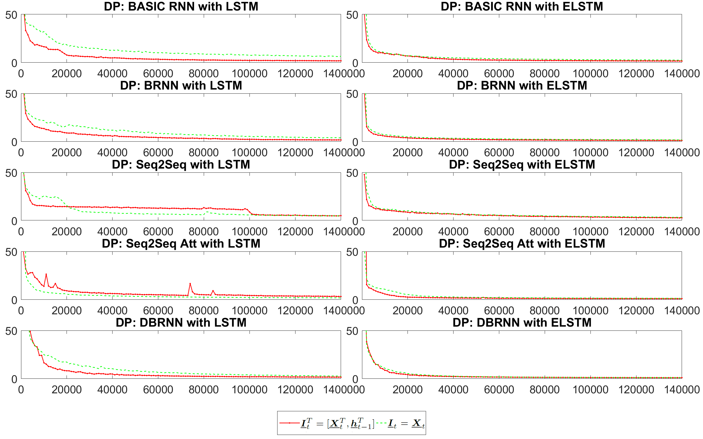
Figure 11: The training perplexity vs. training steps of different models with $\underline{\boldsymbol{I}}_{t}=\underline{\boldsymbol{X}}_{t}$ and $\underline{\boldsymbol{I}}^{T}_{t}=[\underline{\boldsymbol{X}}^{T}_{t},\underline{\boldsymbol{h}}^{T}_{t-1}]$ for the DP task.

5.3 Comparison between ELSTM and Non-RNN-based Methods

As stated earlier, the ELSTM design is more capable of extending the memory and capturing complex SISO relationships than other RNN cells. In this subsection, we compare the DP performance of two models built upon the ELSTM cell (namely, the DBRNN and the seq2seq with attention) and two non-RNN-based neural network based methods (i.e., the TDP [19] and the convseq2seq [2]). The TDP is a hand-crafted method based on a parsing tree, and its neural network is a multi-layer perceptron with one hidden layer. Its neural network is used to predict the transition from a tail word to its headword. The convseq2seq is an end-to-end CNN with an attention mechanism. We used the default settings for the TDP and the convseq2seq as reported in [19] and [2], respectively. For the TDP, we do not use the ground truth POS tags but the predicted dependency relation labels as the input to the parsing tree for the next prediction.

Table 8: DP test accuracy (%) and system settings

	Seq2seq-E	DBRNN-E	Convseq2seq	TDP
UAS	64.30	61.35	52.55	62.29
LAS	52.60	43.32	44.19	52.18
Training steps	11 epochs	11 epochs	11 epochs	11 epochs
# parameters	12,684,468	16,460,468	22,547,124	950,555
Pretrained embedding	No	No	No	Yes
End-to-end	Yes	Yes	Yes	No
Regularization	No	No	No	Yes
Dropout	No	No	Yes	Yes
Optimizer	AdaGrad	AdaGrad	NAG [23]	AdaGrad
Learning rate	0.5	0.5	0.25	0.01
Embedding size	512	512	512	50
Encoder layers	1	N/A	4	N/A
Decoder layers	1	N/A	4	N/A
Kernel size	N/A	N/A	3	N/A
Hidden layer size	N/A	N/A	N/A	200

We see from Table 8 that the ELSTM-based models learn much faster than the CNN-based convseq2seq model with fewer parameters. The convseq2seq uses dropout while the ELSTM-based models do not. It is also observed that convseq2seq does not converge if Adagrad is used as its optimizer. The ELSTM-based seq2seq with attention even outperforms the TDP, which was specifically designed for the DP task. Without a good pretrained word embedding scheme, the UAS and LAS of TDP drop drastically to merely $8.93\%$ and $0.30\%$ respecively.

6 Conclusion and Future Work

Although the memory of the LSTM and GRU celles fades slower than that of the SRN, it is still not long enough for complicated language tasks such as dependency parsing. To address this issue, we proposed the ELSTM to enhance the memory capability of an RNN cell. Besides, we presented a new DBRNN model that has the merits of both the BRNN and the encoder-decoder. It was shown by experimental results that the ELSTM outperforms other RNN cell designs by a significant margin for complex language tasks. The DBRNN model is superior to the BRNN and the seq2seq models for simple and complex language tasks. Furthermore, the ELSTM-based RNN models outperform the CNN-based convseq2seq model and the handcrafted TDP. There are interesting issues to be explored furthermore. For example, is the ELSTM cell also helpful in more sophisticated RNN models such as the deep RNN? Is it possible to make the DBRNN deeper and better? They are left for future study.

7 Declarations of interest

Declarations of interest: none

8 Acknowledgements

This research did not receive any specific grant from funding agencies in the public, commercial, or not-for-profit sectors.

References

Appendix A: More Experimental Results

In the appendix, we compare the training perplexity between $\underline{\boldsymbol{I}}_{t}=\underline{\boldsymbol{X}}_{t}$ and $\underline{\boldsymbol{I}}_{t}^{T}=[\underline{\boldsymbol{X}}_{t}^{T},\underline{\boldsymbol{h}}_{t-1}^{T}]$ for various models with the LSTM, and the ELSTM cells in Fig. 12.

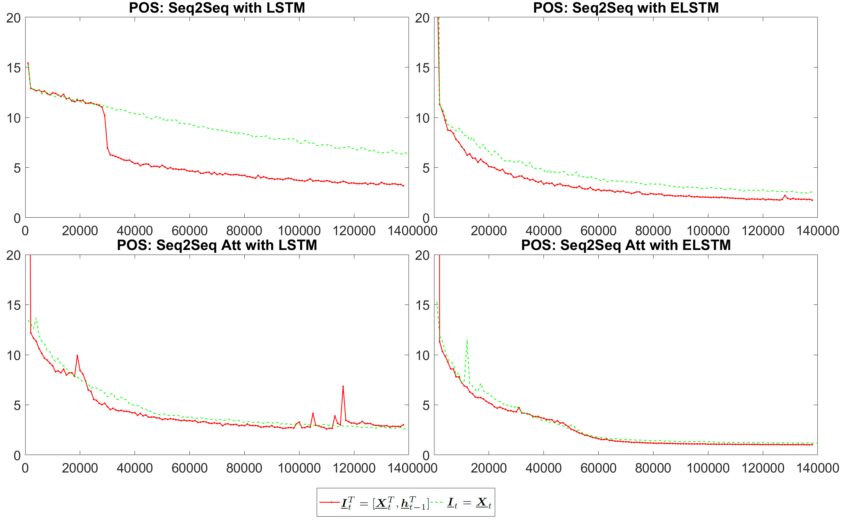
Figure 12: The training perplexity vs. training steps of different models with $\underline{\boldsymbol{I}}_{t}=\underline{\boldsymbol{X}}_{t}$ and $\underline{\boldsymbol{I}}^{T}_{t}=[\underline{\boldsymbol{X}}^{T}_{t},\underline{\boldsymbol{h}}^{T}_{t-1}]$ for the POS tagging task.

References

- [1] H. Cheng, H. Fang, X. He, J. Gao, L. Deng, Bi-directional attention with agreement for dependency parsing, In Proceedings of The Empirical Methods in Natural Language Processing (EMNLP 2016).
- [2] J. Gehring, G. Auli M, D. Yarats, Y. Denis, D. Yann N., Convolutional sequence to sequence learning, in: arXiv preprint, no. 1705.03122, 2017.
- [3] J. Elman, Finding structure in time, Cognitive Science 14 (1990) 179–211.
- [4] M. Jordan, Serial order: A parallel distributed processing approach, Advances in Psychology 121 (1997) 471–495.
- [5] S. Hochreiter, J. Schmidhuber, Long short-term memory, Neural Computation 9 (1997) 1735–1780.
- [6] K. Cho, B. v. Merrienboer, C. Gulcehre, D. Bahdanau, F. Bougares, H. Schwenk, Y. Bengio, Learning phrase representations using RNN encoder–decoder for statistical machine translation, In Proceedings of The Empirical Methods in Natural Language Processing (EMNLP 2014).
- [7] M. Schuster, K. K. Paliwal, Bidirectional recurrent neural networks, Signal Processing 45 (1997) 2673–2681.
- [8] I. Sutskever, O. Vinyals, Q. V. Le, Sequence to sequence learning with neural networks, Advances in Neural Information Processing Systems (2014) 3104–3112.
- [9] O. Vinyals, L. Kaiser, T. Koo, S. Petrov, I. Sutskever, G. Hinton, Grammar as a foreign language, Advances in Neural Information Processing Systems (2015) 2773–2781.
- [10] D. Bahdanau, K. Cho, Y. Bengio, Neural machine translation by jointly learning to align and translate, In Proceedings of the International Conference on Learning Representations (ICLR 2015).
- [11] R. Pascanu, C. Gulcehre, K. Cho, Y. Bengio, How to construct deep recurrent neural networks, arXiv:1312.6026.
- [12] P. Razvan, T. Mikolov, Y. Bengio, On the difficulty of training recurrent neural networks, In Proceedings of The International Conference on Machine Learning (ICML 2013) (2013) 1310–1318.
- [13] Y. Bengio, P. Simard, P. Frasoni, Learning long-term dependencies with gradient descent is difficult, Neural Networks 5 (1994) 157–166.
- [14] F. A. Gers, J. Schmidhuber, F. Cummins, Learning to forget: Continual prediction with lstm, Neural Computation (2000) 2451–2471.
- [15] K. Greff, R. K. Srivastava, J. Koutnik, B. R. Steunebrink, J. Schmidhuber, Lstm: A search space odyssey, IEEE transactions on neural networks and learning systems 28 (10) (2017) 2222–2232.
- [16] J. Chung, C. Gulcehre, K. Cho, Y. Bengio, Empirical evaluation of gated recurrent neural networks on sequence modeling, arXiv preprint (arXiv:1412.3555).
- [17] A. Karpathy, J. Johnson, L. Fei-Fei, Visualizing and understanding recurrent networks, arXiv preprint (arXiv:1506.02078v2).
- [18] J. Hu, L. Shen, G. Sun, Squeeze-and-excitation networks, in: Proceedings of the IEEE conference on computer vision and pattern recognition (CVPR 2018), 2018, pp. 7132–7141.
- [19] D. Chen, M. Christopher, A fast and accurate dependency parser using neural networks, in: In Proceedings of The Empirical Methods in Natural Language Processing (EMNLP 2014), 2014, pp. 740–750.
- [20] M. Marcus, B. Santorini, M. A. Marcinkiewicz, Building a large annotated corpus of english: the penn treebank, Computational Linguistics 19 (1993) 313–330.
- [21] Duchi, Adaptive subgradient methods for online learning and stochastic optimization, The Journal of Machine Learning Research (2011) 2121–2159.
- [22] Y. Bengio, R. Ducharme, P. Vincent, C. Jauvin, A neural probabilistic language model, Journal of Machine Learning Research (2003) 1137–1155.
- [23] Y. Nesterov, A method of solving a convex programming problem with convergence rate o (1/k2), in: Soviet Mathematics Doklady, Vol. 27, 1983, pp. 372–376.