Prony Scenarios and Error Amplification in a Noisy Spike-Train Reconstruction

Abstract

The paper is devoted to the characterization of the geometry of Prony curves arising from spike-train signals. We give a sufficient condition which guarantees the blowing up of the amplitudes of a Prony curve $S$ in case where some of its nodes tend to collide. We also give sufficient conditions on $S$ which guarantee a certain asymptotic behavior of its nodes near infinity.

1 Introduction and Mathematical Background

The main object of study in this paper are spike-train signals $F$ of the form

$$\hskip-190.63338ptF(x)=\sum_{i=1}^{d}a_{i}\delta(x-x_{i}),a_{i},x_{i}\in\mathbb{R}$$ (1.1)

assuming that the number of summands $d$ is known while the values of the amplitudes $A=(a_{1},...,a_{d})$ and the nodes $X=(x_{1},...,x_{d})$ are to be obtained.

Our aim is to find the best approximation of the parameters $a_{1},...,a_{d},x_{1},...,x_{d}$ given the following $q+1$ moments

$$\hskip-142.26378ptm_{k}(F)=\int_{-\infty}^{\infty}x^{k}F(x)dx=\sum_{i=1}^{d}a_{i}x_{i}^{k},k=0,...,q$$ (1.2)

of the signal $F$ where $0\leq q\leq 2d-1$. The system (1.2) is called a Prony system of equations for the signal $F$. In case where $q=2d-1$ we will call the above system a complete Prony system for the parameters $a_{1},...,a_{d},x_{1},...,x_{d}$.

More generally, for each fixed point $\mu=(\mu_{0},...,\mu_{2d-1})\in\mathbb{R}^{2d}$ and $0\leq q\leq 2d-1$ the following system

$$\hskip-270.30118pta_{1}+a_{2}+...+a_{d}=\mu_{0},$$

$$\hskip-234.73523pta_{1}x_{1}+a_{2}x_{2}+...+a_{d}x_{d}=\mu_{1},$$

$$\hskip-312.9803pt...........$$ (1.3)

$$\hskip-234.73523pta_{1}x_{1}^{q}+a_{2}x_{2}^{q}+...+a_{d}x_{d}^{q}=\mu_{q},$$

defines (in the general case) a $2d-q-1$ dimensional algebraic variety $S_{q}(\mu)$ in $\mathbb{R}^{2d}$ where each point $(A,X)\in S_{q}(\mu)$ can be identified with a signal $F$ whose set of amplitudes and nodes are given respectively by the points $A$ and $X$ in $\mathbb{R}^{d}$.

In this paper we will be dealing with the special case where $q=2d-2$ for which $S_{2d-2}(\mu)$ defines, in the general case, a curve in $\mathbb{R}^{2d}$. For this case we assume that $\mu\in\mathbb{R}^{2d-1}$ and define its corresponding Hankel matrix $\mathcal{M}=\mathcal{M}(\mu)$ by

$$\hskip-213.39566pt\mathcal{M}=\left(\begin{array}[]{cccc}\mu_{0}&\mu_{1}&...&\mu_{d-1}\\ \mu_{1}&\mu_{2}&...&\mu_{d}\\ .........\\ \mu_{d-1}&\mu_{d}&...&\mu_{2d-2}\\ \end{array}\right).$$

Observe that if each component of $\mathcal{M}$ is considered as a function of $A$ and $X$, where we replace each value $\mu_{i}$, in the definition of $\mathcal{M}$ above, with its left hand side in the system of equations (1.3), then $\mathcal{M}$ is constant on $S_{2d-2}(\mu)$.

Given a Prony system of equations (1.3), where $q=2d-2$, we will all ways assume that the Hankel matrix $\mathcal{M}$, corresponding to the point $\mu$, is non degenerate. This assumption is necessary since, as we will show later (see Remark 1.3), the degeneracy of the matrix $\mathcal{M}$ is equivalent to the assumption that at least two nodes $x_{i},x_{j}$ where $i\neq j$ collide identically or that at least one amplitude $a_{i}$ vanishes identically on $S_{2d-2}(\mu)$. However, a signal $F$ of the form (1.1) cannot be contained on such curves since this will imply that the number of summands of the signal $F$ is less than $d$.

Prony’s type systems of equations have been investigated by many authors (see [1, 2, 3, 4, 5, 6, 7, 9, 22, 24, 25, 26]) and have been found out to be useful in many fields in applied mathematics such as in imaging in the context of superresolution ([8, 10, 12, 13, 14, 15, 16, 17, 18, 19, 20, 21]) and in approximation theory ([11, 23]). Our motivation in this paper comes from an important result, found in [1], about the worst case errors, in the presence of noise, in the reconstruction of a solution to the complete Prony system and the reconstruction of the Prony curve $S_{2d-2}$.

More specifically, in [1] the authors prove that in case where the nodes $x_{1},...,x_{d}$ form a cluster of size $h\ll 1$, while the measurements error of the acquired moments (1.2) in the presence of noise is of order $\epsilon$, the worst case error in the reconstruction of the solution to the complete Prony system is of order $\epsilon h^{-2d+1}$. However, it is also proved in [1] that the worst case error in the reconstruction of the Prony curve $S_{2d-2}$ is of order $\epsilon h^{-2d+2}$. That is, the reconstruction of the Prony curve $S_{2d-2}$ is $h$ times better than the reconstruction of the solutions themselves and this curve provides a rather accurate prediction of the possible behavior of the noisy reconstructions.

In other words, from the noisy measurements $\mu_{0},...,\mu_{2d-1}$ we can first reconstruct the Prony curve $S_{2d-2}(\mu)$ with the improved accuracy, and then we can consider the curve $S_{2d-2}(\mu)$ as a prediction of a possible distribution of the noisy reconstructions. This scenario includes an accurate description of the behavior of the nodes $x_{j}$ and the amplitudes $a_{j}$ along the curve $S_{2d-2}(\mu)$.

Hence, since the incorrect reconstructions, caused by the measurements noise, are spread along the Prony curve $S_{2d-2}$, our main aim in this paper is to investigate the behavior of the amplitudes on $S_{2d-2}$ in case where some of its nodes tend to collide. We will also investigate the asymptotic behavior of the nodes on $S_{2d-2}$ at infinity.

The main results of this paper are given in Theorems 2.1 and 2.2 in Sect. 2 below. In Theorem 2.1 we prove that in the general case any collision of two nodes $x_{i}$ and $x_{j}$ where $i\neq j$ on a Prony curve $S_{2d-2}(\mu)$ results in the blowing up of their corresponding amplitudes $a_{i}$ and $a_{j}$, that is $|a_{i}|,|a_{j}|\rightarrow\infty$. In Theorem 2.2 we characterize the asymptotic behavior near infinity of the nodes on the Prony curve $S_{2d-2}(\mu)$ and show that in the general case all the nodes are bounded in absolute value except maybe only one node. In Sect. 3 we prove our main results, Theorems 1.1 and 1.2, and in Sect. 4 we investigate the geometry of $S_{2d-2}(\mu)$ for the special cases where $d=2,3$.

Before formulating the main results we will introduce some basic notations, definitions and results concerning Prony curves. Denote by $\mathcal{P}_{d}^{A}$ and $\mathcal{P}_{d}^{X}$ the following sets

$$\hskip-234.73523pt\mathcal{P}_{d}^{A}=\{A=(a_{1},a_{2},...,a_{d})\in\mathbb{R}^{d}\}$$

$$\hskip-129.46011pt\mathcal{P}_{d}^{X}=\{X=(x_{1},x_{2},...,x_{d})\in\mathbb{R}^{d}:x_{1}<x_{2}<...<x_{d}\}$$

which we call the amplitudes parameter space and nodes parameter space respectively. The restriction that $x_{i}<x_{j}$ for $i<j$ is imposed since any permutation of the nodes, and their corresponding amplitudes, of a solution to the Prony system of equations (1.3) is also a solution. Thus, we omit redundant data by taking only one permutation of each set of solutions to (1.3). With this notation we define the parameter space $\mathcal{P}_{d}$ of signals by $\mathcal{P}_{d}=\mathcal{P}_{d}^{A}\times\mathcal{P}_{d}^{X}$, i.e., every signal $F$ given by (1.1) is identified with the point $(A,X)\in\mathcal{P}_{d}$ where $A$ and $X$ denote respectively the amplitudes and nodes vectors of $F$. We also assume that each Prony curve $S_{2d-2}(\mu)$ is contained in $\mathcal{P}_{d}$. We denote by $S_{2d-2}^{X}(\mu)$ the projection of $S_{2d-2}(\mu)$ to the nodes parameter space $\mathcal{P}_{d}^{X}$.

For every $1\leq i\leq d$ define the projection $\pi_{i}:\mathbb{R}^{d}\rightarrow\mathbb{R}^{d-1}$ by

$$\hskip-184.9429pt\pi_{i}(x_{1},...x_{d})=(x_{1},...,x_{i-1},x_{i+1},...,x_{d}).$$

Define the following symmetric polynomials $\varrho_{k},k=1,...,d-1$ and $\sigma_{k},k=1,...,d$ in $\mathbb{R}^{d-1}$ and $\mathbb{R}^{d}$ respectively by :

$$\hskip-68.28644pt\varrho_{k}\left(x_{1},...,x_{d-1}\right)=(-1)^{k}\sum_{1\leq i_{1}<...<i_{k}\leq d-1}x_{i_{1}}...x_{i_{k}},1\leq k\leq d-1,$$

$$\hskip-99.58464pt\sigma_{k}(x_{1},...,x_{d})=(-1)^{k}\sum_{1\leq i_{1}<...<i_{k}\leq d}x_{i_{1}}...x_{i_{k}},1\leq k\leq d.$$

Observe that the symmetric polynomials $\sigma_{1},...,\sigma_{d}$ satisfy, for each $z\in\mathbb{C}$, the following equation

$$Q(z)=(z-x_{1})(z-x_{2})...(z-x_{d})=z^{d}+\sigma_{1}(X)z^{d-1}+...+\sigma_{d-1}(X)z+\sigma_{d}(X)$$ (1.4)

and can be in fact equivalently defined as the unique functions which satisfy equation (1.4) for each complex number $z$. We identify the set of monic polynomials of order $d$ with the space $\mathcal{W}\cong\mathbb{R}^{d}$ where the ordered set $\sigma=(\sigma_{1},...,\sigma_{d})$ of the coefficients of the polynomial $Q$ is identified with $Q$.

By equation (1.4) each fixed point $X$ in $\mathcal{P}_{d}^{X}$ corresponds to a unique set of coefficients $\sigma_{1},...,\sigma_{d}$ and thus to a point $\sigma$ in $\mathcal{W}$. However, not every point $\sigma$ in $\mathcal{W}$ corresponds to a point in $\mathcal{P}_{d}^{X}$ since, as can be seen from equation (1.4), there is no guarantee that all the roots of the polynomial $Q$ are real and distinct if its coefficients are chosen arbitrarily. Hence, we denote by $H_{d}\subset\mathcal{W}$ the subset of hyperbolic polynomials of all points whose components from left to right are the coefficients $\sigma_{1},...,\sigma_{d}$ of a polynomial $Q$, given as in equation (1.4), whose roots are real and distinct. With this notation we define the Vieta mapping

$$\hskip-332.89716pt\mathcal{V}_{d}:\mathcal{P}_{d}^{X}\rightarrow H_{d}$$

$$\hskip-170.71652pt\mathcal{V}_{d}\left(X\right)=\left(\sigma_{1}\left(X\right),...,\sigma_{d}\left(X\right)\right),X=(x_{1},...,x_{d})$$

which is a bijection between $\mathcal{P}_{d}^{X}$ and $H_{d}$.

We will now formulate the following important lemma which is used during the text and its proof is given in the Appendix.

Lemma 1.1.

For $d\leq q\leq 2d-2$ the projection $S_{q}^{X}(\mu)$ of the surface $S_{q}(\mu)$, defined by the system of equations (1.3), into the nodes parameter space $\mathcal{P}_{d}^{X}$ is given by the following system of equations

$$\hskip-146.53151pt\mu_{0}\sigma_{d}\left(X\right)+\mu_{1}\sigma_{d-1}\left(X\right)+...+\mu_{d-1}\sigma_{1}\left(X\right)+\mu_{d}=0,$$

$$\hskip-146.53151pt\mu_{1}\sigma_{d}\left(X\right)+\mu_{2}\sigma_{d-1}\left(X\right)+...+\mu_{d}\sigma_{1}\left(X\right)+\mu_{d+1}=0,$$

$$\hskip-199.16928pt..............$$ (1.5)

$$\hskip-115.23373pt\mu_{q-d}\sigma_{d}\left(X\right)+\mu_{q-d+1}\sigma_{d-1}\left(X\right)+...+\mu_{q-1}\sigma_{1}\left(X\right)+\mu_{q}=0.$$

From Lemma 1.1 it follows that the non degeneracy condition on $\mathcal{M}$ implies that $S_{2d-2}(\mu)$ is a curve in $\mathcal{P}_{d}$. Indeed, by Lemma 1.1 the projection $S_{2d-2}^{X}(\mu)$ to the nodes parameter space $\mathcal{P}_{d}^{X}$ is given by the following system of equations

$$\hskip-36.98866pt\mu_{k}\sigma_{d}\left(X\right)+\mu_{k+1}\sigma_{d-1}\left(X\right)+...+\mu_{k+d-1}\sigma_{1}\left(X\right)=-\mu_{d+k},k=0,...,d-2.$$ (1.6)

Now we ”complete” the system (1.6) by adding the following equation

$$\hskip-156.49014pt\mu_{d-1}\sigma_{d}\left(X\right)+\mu_{d}\sigma_{d-1}\left(X\right)+...+\mu_{2d-2}\sigma_{1}\left(X\right)=t$$ (1.7)

where $t$ is a real parameter. Since $\det\mathcal{M}\neq 0$ it follows that the system of equations obtained by combining the system (1.6) and equation (1.7) is non degenerate. Hence, each one of the variables $\sigma_{1},...,\sigma_{d}$ can be expressed via Cramer’s rule as a linear function of $t$. Explicitly we have

$$\hskip-166.44879pt\sigma_{d-k+1}=\frac{(-1)^{d+k}\mathcal{M}_{d,k}}{\det\mathcal{M}}t+b_{d-k+1},k=1,...,d,$$ (1.8)

where

$$\hskip-31.2982ptb_{d-k+1}=\frac{(-1)^{k}}{\det\mathcal{M}}\left(\mu_{d}\cdot\mathcal{M}_{1,k}-\mu_{d+1}\cdot\mathcal{M}_{2,k}+...+(-1)^{d-2}\mu_{2d-2}\cdot\mathcal{M}_{d-1,k}\right)$$ (1.9)

and where $\mathcal{M}_{i,j}$ denotes the minor of the entry in the $i$-th row and $j$-th column of $\mathcal{M}$. Since the coefficients $\sigma_{1},...,\sigma_{d}$ correspond to $d$ real nodes $x_{1},...,x_{d}$ we take only those values of $t$ for which the line $l_{\mu}$, defined by the parametrization (1.8), is in $H_{d}$. We define $A_{\mu}\subseteq\mathbb{R}$ as the set of all $t\in\mathbb{R}$ for which $l_{\mu}(t)\subset H_{d}$. It can be easily seen that $A_{\mu}$ is a finite union of open intervals in $\mathbb{R}$.

Since the Vieta mapping $\mathcal{V}_{d}$ is a bijection between $H_{d}$ and the nodes parameter space $\mathcal{P}_{d}^{X}$ it follows that each node $x_{i}$ can also be parameterized as a function of $t$ where $t\in A_{\mu}$. For the amplitudes $a_{1},...,a_{d}$ we can solve the first $d$ equations in the system (1.3) which is of Vandermonde’s type if $x\in\mathcal{P}_{d}^{X}$ and express each one of these amplitudes as a function of $x_{1},...,x_{d}$ (and thus as a function of $t$). Hence, we obtained the following proposition.

Proposition 1.2.

Let $\mu$ be a point in $\mathbb{R}^{2d-1}$ and assume that its Hankel matrix $\mathcal{M}(\mu)$ is non degenerate. Then, the set of solutions $S_{2d-2}(\mu)$ in $\mathcal{P}_{d}$ to the system of equations (1.3) for $q=2d-2$ is a curve whose projection $S_{2d-2}^{X}(\mu)$ to $\mathcal{P}_{d}^{X}$ can be parameterized by $\mathcal{V}_{d}^{-1}(\sigma(t)),t\in A_{\mu}$ where $\sigma(t)=(\sigma_{1}(t),...,\sigma_{d}(t))$ is given by equations (1.8)-(1.9).

Remark 1.3.

The assumption that the Hankel matrix $\mathcal{M}$ is non degenerate is equivalent to the assumption that no two nodes $x_{i}$ and $x_{j}$ collide identically and that no amplitude $a_{i}$ vanishes identically on $S_{2d-2}(\mu)$. Indeed, $S_{2d-2}(\mu)$ is defined by the system of equations (1.3), where $q=2d-2$, and this system can be equivalently written in the following matrix form $\mathcal{M}=V\Lambda V^{T}$ where

$$\hskip-71.13188ptV=\left(\begin{array}[]{cccc}1&1&...&1\\ x_{1}&x_{2}&...&x_{d}\\ &.........\\ x_{1}^{d-1}&x_{2}^{d-1}&...&x_{d}^{d-1}\\ \end{array}\right),\Lambda=\left(\begin{array}[]{cccc}a_{1}&0&...&0\\ 0&a_{2}&...&0\\ &..........\\ 0&0&...&a_{d}\\ \end{array}\right).$$ (1.10)

Hence, the degeneracy of $\mathcal{M}$ is equivalent to the degeneracy of the Vandermonde matrix $V$ or of the diagonal matrix $\Lambda$. The degeneracy of $V$ is equivalent to the condition that at least two nodes $x_{i}$ and $x_{j}$, where $i\neq j$, coincide while the degeneracy of $\Lambda$ is equivalent to the condition that at least one of the amplitudes $a_{i}$ vanishes.

Remark 1.4.

Observe that since $S_{2d-2}(\mu)\subset\mathcal{P}_{d}$ it follows in particular that for each point $(A,X)\in S_{2d-2}(\mu)$ we have $X\in\mathcal{P}_{d}^{X}$ and thus collision of two nodes $x_{i}$ and $x_{i+1}$ cannot actually occur on $S_{2d-2}(\mu)$ since $x_{i}<x_{i+1}$. However, when we say that two nodes collide on $S_{2d-2}$ at $t=t_{0}$ and write $x_{i}\sim x_{i+1}$ we mean that $x_{i+1}(t)-x_{i}(t)\rightarrow 0$ as $t\rightarrow t_{0}$ where $t_{0}$ is a boundary point of $A_{\mu}$.

2 Main Results

The first main result, Theorem 2.1, implies that in the general case any collision of two nodes on a Prony curve $S_{2d-2}$ results in the blowing up of their corresponding amplitudes. The exact formulation is as follows:

Theorem 2.1.

Let $\mu$ be a point in $\mathbb{R}^{2d-1}$ and assume that its corresponding Hankel matrix $\mathcal{M}$ is non degenerate. Then, if the nodes $x_{i}(t)$ and $x_{i+1}(t)$ tend to collide on $S_{2d-2}(\mu)$ as $t\rightarrow t_{0}$, where $1\leq i\leq d-1$, then the amplitudes $a_{i}(t)$ and $a_{i+1}(t)$ tend to infinity as $t\rightarrow t_{0}$.

The second main result, Theorem 2.2, implies that in the general case only one node on a Prony curve $S_{2d-2}$ can approach to infinity at a time. The exact formulation is as follows:

Theorem 2.2.

Assume that the Hankel matrix $\mathcal{M}$, of a point $\mu\in\mathbb{R}^{2d-1}$, and its top-left $(d-1)\times(d-1)$ sub matrix are non degenerate. Let $A_{\mu}^{\prime}\subset A_{\mu}$ be an unbounded interval of $A_{\mu}$ and let

$$\hskip-184.9429pt\gamma(t)=(x_{1}(t),x_{2}(t),...,x_{d}(t)),t\in A_{\mu}^{\prime}$$

be the parametrization, of a connected component of $S_{2d-2}^{X}$, given as in Proposition 1.2 which is now restricted on $A_{\mu}^{\prime}$. That is, $\gamma(t)=\mathcal{V}_{d}^{-1}(\sigma(t)),t\in A_{\mu}^{\prime}$ where $\sigma(t)$ is given by equations (1.8)-(1.9). Then, as $t\rightarrow\infty$ (or $t\rightarrow-\infty$) in $A_{\mu}^{\prime}$ at most one node $x_{i}=x_{i}(t)$ tends to infinity.

3 Proofs of the Main Results

Proof of Theorem 2.1: First observe that if two nodes tend to collide on the Prony curve $S_{2d-2}(\mu)$ then it follows immediately, from the factorization $\mathcal{M}=V\Lambda V^{T}$ where $V$ and $\Lambda$ are given by (1.10), that at least one amplitude must tend to infinity. Indeed, if $t_{0}$ is a point for which $x_{i+1}(t)-x_{i}(t)\rightarrow 0$ as $t\rightarrow t_{0}$ then from the definition of the matrix $V$ we have that $\det V(t)\rightarrow 0$. Hence, it follows that

$$\hskip-92.47145pt|a_{1}(t)|...|a_{d}(t)|=|\det\Lambda(t)|=\left|\frac{\det\mathcal{M}}{(\det V(t))^{2}}\right|\rightarrow\infty\hskip 7.11317pt\mathrm{as}\hskip 7.11317ptt\rightarrow t_{0}$$ (3.1)

since by assumption $\det\mathcal{M}\neq 0$. Hence, from equation (3.1) there exists an amplitude $a_{j}$ satisfying $|a_{j}(t)|\rightarrow\infty$ as $t\rightarrow t_{0}$. However, from the above analysis it is still not clear which amplitudes must tend to infinity where our goal is to prove that these are the amplitudes $a_{i}$ and $a_{i+1}$ corresponding to the nodes $x_{i}$ and $x_{i+1}$.

For this we will have to express the amplitudes $a_{k},k=1,2,...,d$ in terms of $x_{i},i=1,2,...,d$. Observe that the first $d$ equations in the system (1.3) can be rewritten as follows

$$\hskip-128.0374pt\left(\begin{array}[]{cccc}1&1&...&1\\ x_{1}&x_{2}&...&x_{d}\\ ........\\ x_{1}^{d-1}&x_{2}^{d-1}&...&x_{d}^{d-1}\end{array}\right)\left(\begin{array}[]{c}a_{1}\\ a_{2}\\ ...\\ a_{d}\end{array}\right)=\left(\begin{array}[]{c}\mu_{0}\\ \mu_{1}\\ ...\\ \mu_{d-1}\end{array}\right).$$

Using the well known formula for the inverse of the Vandermonde’s matrix (see, for example [27]) we obtain from the last matrix equation that

$$\hskip-42.67912pt\left(\begin{array}[]{c}a_{1}\\ a_{2}\\ ...\\ a_{d}\end{array}\right)=\left(\begin{array}[]{ccccc}\frac{\varrho_{d-1}(\pi_{1}(X))}{L_{1}(X)}&\frac{\varrho_{d-2}(\pi_{1}(X))}{L_{1}(X)}&...&\frac{\varrho_{1}(\pi_{1}(X))}{L_{1}(X)}&\frac{1}{L_{1}(X)}\\ \frac{\varrho_{d-1}(\pi_{2}(X))}{L_{2}(X)}&\frac{\varrho_{d-2}(\pi_{2}(X))}{L_{2}(X)}&...&\frac{\varrho_{1}(\pi_{2}(X))}{L_{2}(X)}&\frac{1}{L_{2}(X)}\\ ..........\\ \frac{\varrho_{d-1}(\pi_{d}(X))}{L_{d}(X)}&\frac{\varrho_{d-2}(\pi_{d}(X))}{L_{d}(X)}&...&\frac{\varrho_{1}(\pi_{d}(X))}{L_{d}(X)}&\frac{1}{L_{d}(X)}\\ \end{array}\right)\left(\begin{array}[]{c}\mu_{0}\\ \mu_{1}\\ ...\\ \mu_{d-1}\end{array}\right)$$ (3.2)

where

$$\hskip-256.0748ptL_{k}(X)=\underset{i\neq k}{\overset{d}{\underset{i=1}{\prod}}}(x_{k}-x_{i}).$$

Let us assume without loss of generality that the nodes $x_{d-1}$ and $x_{d}$ collide on $S_{2d-2}(\mu)$, we will show that $a_{d-1}$ and $a_{d}$ tend to infinity in this case. Also, from the symmetry of the formulas for $a_{d-1}$ and $a_{d}$ in terms of the nodes $x_{1},x_{2},...,x_{d}$ it will be enough to prove our assertion only for $a_{d}$. Hence, we will concentrate from now on only on this amplitude.

For the amplitude $a_{d}$ we define the following polynomial

$$\hskip-341.43306ptP(x_{1},x_{2},...,x_{d-1})$$

$$\hskip-28.45274pt=\mu_{0}\varrho_{d-1}(x_{1},...,x_{d-1})+\mu_{1}\varrho_{d-2}(x_{1},...,x_{d-1})+...+\mu_{d-2}\varrho_{1}(x_{1},...,x_{d-1})+\mu_{d-1}.$$

By equation (3.2) we have

$$\hskip-184.9429pta_{d}(x_{1},...,x_{d})=\frac{P(x_{1},...,x_{d-1})}{(x_{d}-x_{1})...(x_{d}-x_{d-1})}$$

and thus if a point $(x_{1},x_{2},...,x_{d})\in S_{2d-2}^{X}(\mu)$ satisfies that its nodes $x_{d-1}$ and $x_{d}$ tend to collide then $a_{d}$ must tend to infinity unless the polynomial $P$ vanishes at this point (in which case $a_{d}$ may or may not tend to infinity). By Lemma 1.1 the curve $S_{2d-2}^{X}(\mu)$ is defined by the following system of equations

$$\hskip-98.16191pt\mu_{d-1}(x_{1}+x_{2}+...+x_{d})-\mu_{d-2}(x_{1}x_{2}+x_{1}x_{3}+...+x_{d-1}x_{d})$$

$$\hskip 56.9055pt+...+(-1)^{d-1}\mu_{0}x_{1}x_{2}...x_{d}=\mu_{d},$$

$$\hskip-108.12054pt\mu_{d}(x_{1}+x_{2}+...+x_{d})-\mu_{d-1}(x_{1}x_{2}+x_{1}x_{3}+...+x_{d-1}x_{d})$$

$$\hskip 68.28644pt+...+(-1)^{d-1}\mu_{1}x_{1}x_{2}...x_{d}=\mu_{d+1},$$

$$\hskip-199.16928pt...................$$

$$\hskip-85.35826pt\mu_{2d-3}(x_{1}+x_{2}+...+x_{d})-\mu_{2d-4}(x_{1}x_{2}+x_{1}x_{3}+...+x_{d-1}x_{d})$$

$$\hskip 88.2037pt+...+(-1)^{d-1}\mu_{d-2}x_{1}x_{2}...x_{d}=\mu_{2d-2}.$$

By our assumption we have $x_{d}\sim x_{d-1}$ and thus the last system of equations can be rewritten as

$$\hskip-14.22636pt\mu_{d-1}(x_{d-1}+x_{1}+...+x_{d-1})-\mu_{d-2}((x_{1}+...+x_{d-1})\cdot x_{d-1}+x_{1}x_{2}+x_{1}x_{3}$$

$$\hskip-93.89418pt+...+x_{d-2}x_{d-1})+...+(-1)^{d-1}\mu_{0}(x_{1}x_{2}...x_{d-1})\cdot x_{d-1}=\mu_{d},$$

$$\hskip-19.91684pt\mu_{d}(x_{d-1}+x_{1}+...+x_{d-1})-\mu_{d-1}((x_{1}+...+x_{d-1})\cdot x_{d-1}+x_{1}x_{2}+x_{1}x_{3}$$

$$\hskip-85.35826pt+...+x_{d-2}x_{d-1})+...+(-1)^{d-1}\mu_{1}(x_{1}x_{2}...x_{d-1})\cdot x_{d-1}=\mu_{d+1},$$

$$\hskip-227.62204pt...................$$ (3.3)

$$\hskip-5.69046pt\mu_{2d-3}(x_{d-1}+x_{1}+...+x_{d-1})-\mu_{2d-4}((x_{1}+...+x_{d-1})\cdot x_{d-1}+x_{1}x_{2}+x_{1}x_{3}$$

$$\hskip-71.13188pt+...+x_{d-2}x_{d-1})+...+(-1)^{d-1}\mu_{d-2}(x_{1}x_{2}...x_{d-1})\cdot x_{d-1}=\mu_{2d-2}.$$

Hence, it will be enough to show that if a point $X^{\ast}=(x_{1},x_{2},...,x_{d-1})$ in $\mathbb{R}^{d-1}$ satisfies the system of equations (3.3) then $P(X^{\ast})\neq 0$. Suppose that this is not the case, then there exists a point $X^{\ast}\in\mathbb{R}^{d-1}$ which satisfies the system of equations (3.3) and is also a zero of the polynomial $P$. In terms of the symmetric polynomials $\varrho_{1},...,\varrho_{d-1}$ the last condition can be written as

$$\hskip-110.96556pt\mu_{d-1}(x_{d-1}-\varrho_{1}(X^{\ast}))+\mu_{d-2}(\varrho_{1}(X^{\ast})x_{d-1}-\varrho_{2}(X^{\ast}))$$

$$\hskip-17.07182pt+...+\mu_{1}(\varrho_{d-2}(X^{\ast})x_{d-1}-\varrho_{d-1}(X^{\ast}))+\mu_{0}\varrho_{d-1}(X^{\ast})x_{d-1}=\mu_{d},$$

$$\hskip-119.50148pt\mu_{d}(x_{d-1}-\varrho_{1}(X^{\ast}))+\mu_{d-1}(\varrho_{1}(X^{\ast})x_{d-1}-\varrho_{2}(X^{\ast}))$$

$$\hskip-5.69046pt+...+\mu_{2}(\varrho_{d-2}(X^{\ast})x_{d-1}-\varrho_{d-1}(X^{\ast}))+\mu_{1}\varrho_{d-1}(X^{\ast})x_{d-1}=\mu_{d+1},$$

$$\hskip-170.71652pt.............$$ (3.4)

$$\hskip-102.43008pt\mu_{2d-3}(x_{d-1}-\varrho_{1}(X^{\ast}))+\mu_{2d-4}(\varrho_{1}(X^{\ast})x_{d-1}-\varrho_{2}(X^{\ast}))$$

$$\hskip 19.91684pt+...+\mu_{d-1}(\varrho_{d-2}(X^{\ast})x_{d-1}-\varrho_{d-1}(X^{\ast}))+\mu_{d-2}\varrho_{d-1}(X^{\ast})x_{d-1}=\mu_{2d-2},$$

$$\hskip-113.81102pt-\mu_{d-2}\varrho_{1}(X^{\ast})-\mu_{d-3}\varrho_{2}(X^{\ast})-...-\mu_{0}\varrho_{d-1}(X^{\ast})=\mu_{d-1}.$$

From the last equation of the system (3.4) we have the following equality

$$\hskip-42.67912pt\mu_{0}\varrho_{d-1}(X^{\ast})=-\mu_{1}\varrho_{d-2}(X^{\ast})-...-\mu_{d-3}\varrho_{2}(X^{\ast})-\mu_{d-2}\varrho_{1}(X^{\ast})-\mu_{d-1}.$$

Inserting this equality into the first equation of the system (3.4) we have

$$\mu_{d}=\mu_{d-1}(x_{d-1}-\varrho_{1}(X^{\ast}))+\mu_{d-2}(\varrho_{1}(X^{\ast})x_{d-1}-\varrho_{2}(X^{\ast}))+...+\mu_{1}(\varrho_{d-2}(X^{\ast})x_{d-1}-\varrho_{d-1}(X^{\ast}))$$

$$\hskip-85.35826pt+\left(-\mu_{1}\varrho_{d-2}(X^{\ast})-...-\mu_{d-3}\varrho_{2}(X^{\ast})-\mu_{d-2}\varrho_{1}(X^{\ast})-\mu_{d-1}\right)x_{d-1}.$$

Observe that all the terms which contain a product of a symmetric polynomial with the node $x_{d-1}$ cancel each other. Hence we are left with the following equality

$$\hskip-142.26378pt-\mu_{d-1}\varrho_{1}(X^{\ast})-\mu_{d-2}\varrho_{2}(X^{\ast})-...-\mu_{1}\varrho_{d-1}(X^{\ast})=\mu_{d}.$$

From the last equation we have the following equality

$$\hskip-85.35826pt\mu_{1}\varrho_{d-1}(X^{\ast})=-\mu_{2}\varrho_{d-2}(X^{\ast})-...-\mu_{d-2}\varrho_{2}(X^{\ast})-\mu_{d-1}\varrho_{1}(X^{\ast})-\mu_{d}.$$

Inserting this equality into the second equation of the system (3.4) we have

$$\mu_{d+1}=\mu_{d}(x_{d-1}-\varrho_{1}(X^{\ast}))+\mu_{d-1}(\varrho_{1}(X^{\ast})x_{d-1}-\varrho_{2}(X^{\ast}))+...+\mu_{2}(\varrho_{d-2}(X^{\ast})x_{d-1}-\varrho_{d-1}(X^{\ast}))$$

$$\hskip-85.35826pt+\left(-\mu_{2}\varrho_{d-2}(X^{\ast})-...-\mu_{d-2}\varrho_{2}(X^{\ast})-\mu_{d-1}\varrho_{1}(X^{\ast})-\mu_{d}\right)x_{d-1}.$$

Again, observe that all the terms which contain a product of a symmetric polynomial with the node $x_{d-1}$ cancel each other. Hence we are left with the following equality

$$\hskip-142.26378pt-\mu_{d}\varrho_{1}(X^{\ast})-\mu_{d-1}\varrho_{2}(X^{\ast})-...-\mu_{2}\varrho_{d-1}(X^{\ast})=\mu_{d+1}.$$

Continuing in this way we can extract from the system of equations (3.4) the following system

$$\hskip-89.626pt-\mu_{d+k-2}\varrho_{1}(X^{\ast})-\mu_{d+k-3}\varrho_{2}(X^{\ast})-...-\mu_{k}\varrho_{d-1}(X^{\ast})=\mu_{d+k-1}$$

where $k=0,...,d-1$. The last system of equations can be written in the following matrix form

$$\left(\begin{array}[]{ccccc}\mu_{0}&\mu_{1}&...&\mu_{d-2}&\mu_{d-1}\\ \mu_{1}&\mu_{2}&...&\mu_{d-1}&\mu_{d}\\ &.........\\ \mu_{d-1}&\mu_{d}&...&\mu_{2d-3}&\mu_{2d-2}\\ \end{array}\right)\left(\begin{array}[]{c}\varrho_{d-1}(X^{\ast})\\ \varrho_{d-2}(X^{\ast})\\ ........\\ \varrho_{1}(X^{\ast})\\ 1\end{array}\right)=\left(\begin{array}[]{c}0\\ 0\\ ...\\ 0\\ 0\end{array}\right).$$

Since, by our main assumption, the matrix in the left hand side of the last equation is non degenerate and hence we obviously arrive to a contradiction. Thus, if a point $X^{\ast}=(x_{1},x_{2},...,x_{d-1})$ in $\mathbb{R}^{d-1}$ satisfies the system of equations (3.3) then $P(X^{\ast})\neq 0$ and hence $a_{d}$ tends to infinity. This proves Theorem 2.1.                                            $\square$

Proof of Theorem 2.2: From Proposition 1.2 we know that the symmetric polynomials $\sigma_{1},...,\sigma_{d}$ can be parameterized on $S_{2d-2}^{X}$ as follows

$$\hskip-142.26378pt\sigma_{d-k+1}=\frac{(-1)^{d+k}\mathcal{M}_{d,k}}{\det\mathcal{M}}t+b_{d-k+1},t\in A_{\mu},k=1,...,d$$

where $b_{k},k=1,...,d$ are constants which depend only on $\mu$ and are independent of $t$ (see formula (1.9)) and where $\mathcal{M}_{i,j}$ denotes the minor of the entry in the $i$-th row and $j$-th column of the matrix $\mathcal{M}$. Since, by assumption, $\mathcal{M}_{d,d}\neq 0$, Theorem 2.2 is a consequence of the following proposition.

Proposition 3.1.

Let $x_{1}=x_{1}(t),...,x_{n}=x_{n}(t),t\in\mathbb{R}$ be $n$ continuous functions which satisfy the following identities

$$\sigma_{k}(X(t))=(-1)^{k}\sum_{1\leq i_{1}<i_{2}<...<i_{k}\leq n}x_{i_{1}}(t)x_{i_{2}}(t)...x_{i_{k}}(t)=a_{k}t+b_{k},k=1,...,n$$ (3.5)

where $a_{k},b_{k}\in\mathbb{R}$ and $a_{1}\neq 0$. Then, as $t\rightarrow\pm\infty$ there is at most one function $x_{i}=x_{i}(t)$ which tends to infinity.

Before proving Proposition 3.1 we need the following lemma which is a direct consequence of the Budan-Fourier Theorem:

Lemma 3.2.

For any polynomial $P$ of degree $n$ and a point $x\in\mathbb{R}$, if $\nu_{P}(x)$ denotes the number of sign changes in the components of the vector $(P(x),P^{\prime}(x),...,P^{(n)}(x))$ then the number of zeros of $P$ with multiplicity in the interval $(a,b]$ is less than or equal to $\nu_{P}(a)-\nu_{P}(b)$.

Proof of Proposition 3.1: We can assume with out loss of generality that $a_{1}>0$ since otherwise we can replace each $x_{i}$ with $-x_{i}$. Observe that from equation (3.5) it follows that for each $\lambda\in\mathbb{R}$ we have

$$(\lambda-x_{1}(t))(\lambda-x_{2}(t))...(\lambda-x_{n}(t))=\lambda^{n}+(a_{1}t+b_{1})\lambda^{n-1}+...+a_{n}t+b_{n}.$$ (3.6)

Hence, if we denote by $P_{t}=P_{t}(\lambda)$ the polynomial in the right hand side of equation (3.6) then we need to prove that as $t\rightarrow\infty$ (or $t\rightarrow-\infty$) all the roots of $P_{t}$ will be bounded except maybe only one root. Observe that by Lemma 3.2 the number of roots of the polynomial $P_{t}$ at the ray $(\lambda,\infty)$ is less than or equal to $\nu_{P_{t}}(\lambda)-\nu_{P_{t}}(\infty)$. Since obviously $\nu_{P_{t}}(\infty)=0$ we only need to estimate $\nu_{P_{t}}(\lambda)$. Explicitly we have

$$\hskip-256.0748pt(P_{t}(\lambda),P_{t}^{\prime}(\lambda),...,P_{t}^{(n)}(\lambda))^{T}$$

$$=\left(\begin{array}[]{c}\hskip-150.79968pt\lambda^{n}+b_{1}\lambda^{n-1}+...+b_{n}+(a_{1}\lambda^{n-1}+a_{2}\lambda^{n-2}+...+a_{n})t\\ n\lambda^{n-1}+(n-1)b_{1}\lambda^{n-2}+...+b_{n-1}+\left[(n-1)a_{1}\lambda^{n-2}+(n-2)a_{2}\lambda^{n-3}+...+a_{n-1}\right]t\\ \hskip-332.89716pt...........................\\ \hskip-293.06346ptn!\lambda+(n-1)!\cdot(a_{1}t+b_{1})\\ \hskip-411.8538ptn!\end{array}\right)$$

$$\hskip-275.99164pt=\left(\begin{array}[]{c}\hskip-45.52458ptR(\lambda)+Q(\lambda)t\\ \hskip-42.67912ptR^{\prime}(\lambda)+Q^{\prime}(\lambda)t\\ \hskip-73.97733pt..........\\ R^{(n-1)}(\lambda)+Q^{(n-1)}(\lambda)t\\ \hskip-79.6678ptR^{(n)}(\lambda)\\ \end{array}\right)$$ (3.7)

where

$$\hskip-28.45274ptR(\lambda)=\lambda^{n}+b_{1}\lambda^{n-1}+...+b_{n},Q(\lambda)=a_{1}\lambda^{n-1}+a_{2}\lambda^{n-2}+...+a_{n}.$$

Observe that if for $\lambda\in\mathbb{R}$ we have $Q(\lambda)>0,...,Q^{(n-1)}(\lambda)>0$ then obviously by taking $t$ large enough all the components of the vector defined by (3.7) will be positive and thus $\nu_{P_{t}}(\lambda)=0$. Since $a_{1}>0$ it follows that for each $k$ there exists $\lambda_{k}$ such that $Q^{(k)}(x)>0$ for $x\geq\lambda_{k}$. Hence, by choosing $\lambda^{\prime}=\max(\lambda_{0},...,\lambda_{n-1})$ and $t$ large enough all the components of the vector (3.7) will be positive and thus $\nu_{P_{t}}(\lambda)=0,\forall\lambda\geq\lambda^{\prime}$ which will imply in particular that for $t$ large enough the polynomial $P_{t}=P_{t}(\lambda)$ does not have any roots for $\lambda\geq\lambda^{\prime}$ where $\lambda^{\prime}$ does not depend on $t$. Hence, at this point we proved that non of the roots $x_{i}=x_{i}(t)$ can tend to $+\infty$ as $t\rightarrow\infty$. We need to check how many roots can tend to $-\infty$ as $t\rightarrow\infty$.

For any $\lambda\in\mathbb{R}$ observe that by Lemma 3.2 the number of roots of the polynomial $P_{t}$ at the ray $(-\infty,\lambda)$ is less than or equal to $\nu_{P_{t}}(-\infty)-\nu_{P_{t}}(\lambda)=n-\nu_{P_{t}}(\lambda)$. Our aim now is to choose $\lambda$ such that the vector (3.7) will have exactly $n-1$ sign changes (and thus $\nu_{P_{t}}(\lambda)=n-1$). Observe that since $a_{1}>0$ we can choose as before $\lambda$ in $\mathbb{R}$ which is small enough and which does not depend on $t$ such that

$$Q(\lambda)>0,Q^{\prime}(\lambda)<0,Q^{\prime\prime}(\lambda)>0,...,Q^{(n-2)}<0,Q^{(n-1)}(\lambda)>0$$

or

$$Q(\lambda)<0,Q^{\prime}(\lambda)>0,Q^{\prime\prime}(\lambda)<0,...,Q^{(n-2)}<0,Q^{(n-1)}(\lambda)>0$$

where the first case corresponds to the case where $n$ is odd and the second case corresponds to the case where $n$ is even. Thus, by taking $t$ large enough the signs of the vector (3.7) will have the form $(+-+-...+-++)$ or the form $(-+-+...-+-++)$. In either case the vector (3.7) will have exactly $n-1$ sign changes and thus $\nu_{P_{t}}(\lambda)=n-1$. Thus, from Lemma 3.2 it follows that the polynomial $P_{t}$ has at most $\nu_{P_{t}}(-\infty)-\nu_{P_{t}}(\lambda)=n-(n-1)=1$ roots at the ray $(-\infty,\lambda)$. This implies that only one of the functions $x_{i}=x_{i}(t)$ can tend to $-\infty$ as $t\rightarrow\infty$. Hence we proved Proposition 3.1 for the case where $t\rightarrow\infty$.

If $t\rightarrow-\infty$ we can just replace each function $x_{i}=x_{i}(t)$ with $y_{i}=y_{i}(t)=x_{i}(-t)$ and use the fact that the functions $y_{i},i=1,...,n$ satisfy a similar set of equations as (3.5). $\hskip 392.64812pt\square$

It can be proved from the Budan-Fourier Theorem that in fact the number of roots of a polynomial $P$ at the interval $(a,b]$ is equal to $\nu_{P}(a)-\nu_{P}(b)-2k$ where $k$ is a nonnegative integer. Hence, from the proof of Proposition 3.1 we have the following corollary.

Corollary 3.3.

Let $x_{1}=x_{1}(t),...,x_{n}=x_{n}(t),t\in\mathbb{R}$ be $n$ continuous functions which satisfy the set of identities (3.5) where $a_{k},b_{k}\in\mathbb{R}$ and $a_{1}\neq 0$. Then, as $t\rightarrow\infty$ (or $t\rightarrow-\infty$) there is exactly one function $x_{i}=x_{i}(t)$ which tends to infinity.

4 The Special Cases $d=2,3$

For the special cases where $d=2,3$ we would like to analyse the projections $S_{2d-2}^{X}$, of the Prony curves $S_{2d-2}$, to the nodes parameter space $\mathcal{P}_{d}^{X}$ and answer the following two questions: A. For which points $\mu\in\mathbb{R}^{2d-1}$ collision of nodes on $S_{2d-2}^{X}(\mu)$ actually occurs? B. For which points $\mu\in\mathbb{R}^{2d-1}$ the projections $S_{2d-2}^{X}(\mu)$ are bounded? We also give some examples to illustrate the main results obtained in Sect. 3. We will always assume that the corresponding Hankel matrix $\mathcal{M}$ for the vector $\mu$ is non degenerate.

The case $d=2$: For $d=2$, $S_{2}(\mu)$ is given as the set of solutions to the following system of equations

$$\hskip-305.86711pta_{1}+a_{2}=\mu_{0},$$

$$\hskip-284.52756pta_{1}x_{1}+a_{2}x_{2}=\mu_{1},$$

$$\hskip-287.373pta_{1}x_{1}^{2}+a_{2}x_{2}^{2}=\mu_{2}$$

and the determinant of its corresponding Hankel matrix $\mathcal{M}$ is given by

$$\hskip-207.7052pt\det\mathcal{M}=\left|\begin{array}[]{cc}\mu_{0}&\mu_{1}\\ \mu_{1}&\mu_{2}\end{array}\right|=\mu_{0}\mu_{2}-\mu_{1}^{2}.$$

By Lemma 1.1 the projection $S_{2}^{X}(\mu)$ of $S_{2}(\mu)$ to the nodes parameter space $\mathcal{P}_{2}^{X}(\mu)$ is given by

$$\hskip-210.55022pt\mu_{0}x_{1}x_{2}-\mu_{1}(x_{1}+x_{2})+\mu_{2}=0.$$ (4.1)

In order to determine for which points $\mu=(\mu_{0},\mu_{1},\mu_{2})$ there is a collision of nodes observe that in terms of the symmetric polynomials $\sigma_{1}$ and $\sigma_{2}$ the nodes $x_{1}$ and $x_{2}$ collide if and only if the polynomial

$$\hskip-167.87108ptQ(z)=(z-x_{1})(z-x_{2})=z^{2}+\sigma_{1}z+\sigma_{2}$$

has a double root which occurs if and only if its discriminant $\triangle(\sigma_{1},\sigma_{2})=\sigma_{1}^{2}-4\sigma_{2}$ vanishes. Hence, in the terms of the symmetric polynomials it follows from equation (4.1) that a collusion of nodes occurs if and only if the line

$$\hskip-264.6107pt\mu_{0}\sigma_{2}+\mu_{1}\sigma_{1}+\mu_{2}=0$$ (4.2)

intersects the parabola $\triangle(\sigma_{1},\sigma_{2})=0$. An intersection occurs if and only if the following equation

$$\hskip-256.0748pt\mu_{0}\sigma_{1}^{2}+4\mu_{1}\sigma_{1}+4\mu_{2}=0$$

has at least one real root which, in case where $\det\mathcal{M}\neq 0$, occurs if and only if $\det\mathcal{M}=\mu_{0}\mu_{2}-\mu_{1}^{2}<0$. This answers Question A for $d=2$.

In order to determine for which points $\mu=(\mu_{0},\mu_{1},\mu_{2})$ the projection $S_{2}^{X}(\mu)$ is bounded observe that in terms of the symmetric polynomials $\sigma_{1}$ and $\sigma_{2}$ each point $x$ in $S_{2}^{X}(\mu)$ corresponds, by the Vieta mapping, to a point $(\sigma_{1},\sigma_{2})$ on the line (4.2) for which $\triangle(\sigma_{1},\sigma_{2})>0$. Since the intersection of the line (4.2) and the set $\triangle(\sigma_{1},\sigma_{2})>0$ is never bounded (unless $\mu_{0}=\mu_{1}=0,\mu_{2}\neq 0$ for which $\det\mathcal{M}=0$) and the Vieta mapping maps bounded sets into bounded sets it follows that the inverse image of this intersection, i.e. the set $S_{2}^{X}(\mu)$, is also unbounded. Hence, there are no points $\mu\in\mathbb{R}^{3}$ for which $S_{2}^{X}(\mu)$ is bounded in case where $\det\mathcal{M}\neq 0$. This answers Question B for the case $d=2$.

Example 4.1.

Let us illustrate Theorem 2.1 for the case $d=2$. For $\mu=(0,1,0)$ the Prony curve $S_{2}(\mu)$ is given by the following system of equations

$$\hskip-321.51622pta_{1}+a_{2}=0,$$

$$\hskip-298.75394pta_{1}x_{1}+a_{2}x_{2}=1,$$

$$\hskip-298.75394pta_{1}x_{1}^{2}+a_{2}x_{2}^{2}=0.$$

Observe that

$$\hskip-241.84842pt\left|\begin{array}[]{cc}\mu_{0}&\mu_{1}\\ \mu_{1}&\mu_{2}\end{array}\right|=\left|\begin{array}[]{cc}0&1\\ 1&0\end{array}\right|\neq 0.$$

Hence, one can expect that if the two nodes $x_{1}$ and $x_{2}$ collide on $S_{2}(\mu)$ then the amplitudes $a_{1}$ and $a_{2}$ will tend to infinity. By using some elementary algebraic manipulations one can show that $S_{2}(\mu)$ has the following parametrization

$$\hskip-184.9429ptS_{2}(\mu)=\left\{\left(-\frac{1}{2t},\frac{1}{2t},-t,t\right):t>0\right\}.$$

Observe that the nodes $x_{1}$ and $x_{2}$ collide as $t\rightarrow 0^{+}$ in which case the amplitudes indeed tend to infinity.

Example 4.2.

Figure 1 below illustrates the projections $S_{2}^{X}(\mu)$ (drawn in red) to $\mathcal{P}_{d}^{X}$ of the Prony curves $S_{2}(\mu)$ for four different points $\mu=(\mu_{0},\mu_{1},\mu_{2})\in\mathbb{R}^{3}$ (we draw in blue the projections to the nodes parameter space $\{(x_{1},x_{2}):x_{2}<x_{1}\}$). The images of these projections under the Vieta mapping $\mathcal{V}_{d}$ are the lines given in the upper part of Figure 1 and, as we have just proved, each intersection of a line $l$ with the parabola $\triangle(\sigma_{1},\sigma_{2})=0$ corresponds to a collision of nodes in the preimage $\mathcal{V}_{d}^{-1}(l)$ as Figure 1 shows.

Observe also that, as accordance with Theorem 2.2, on the curves which are the connected components of any projection $S_{2}^{X}(\mu)$ to the nodes parameter space $\mathcal{P}_{d}^{X}$ only one node tends to infinity at a time except from the last case $x_{1}+x_{2}-1=0$ where $\mu_{0}=0$ for which the sufficient condition of Theorem 2.2 is not satisfied. In fact, the only cases for which the nodes $x_{1}$ and $x_{2}$ on $S_{2}^{X}(\mu)$ tend simultaneously to $\pm\infty$ occur when $\mu_{0}=0$ or equivalently when the image of a projection $S_{2}^{X}(\mu)$, under the Vieta mapping $\mathcal{V}_{d}$, is contained in a vertical line.

The case $d=3$: For $d=3$, $S_{4}(\mu)$ is given as the set of solutions to the following system of equations

$$\hskip-275.99164pta_{1}+a_{2}+a_{3}=\mu_{0},$$

$$\hskip-241.84842pta_{1}x_{1}+a_{2}x_{2}+a_{3}x_{3}=\mu_{1},$$

$$\hskip-241.84842pta_{1}x_{1}^{2}+a_{2}x_{2}^{2}+a_{3}x_{3}^{2}=\mu_{2},$$

$$\hskip-241.84842pta_{1}x_{1}^{3}+a_{2}x_{2}^{3}+a_{3}x_{3}^{3}=\mu_{3},$$

$$\hskip-244.69386pta_{1}x_{1}^{4}+a_{2}x_{2}^{4}+a_{3}x_{3}^{4}=\mu_{4}$$

and by Lemma 1.1 the projection $S_{4}^{X}(\mu)$ of $S_{4}(\mu)$ to the nodes parameter space $\mathcal{P}_{3}^{X}(\mu)$ is given by

$$\hskip-42.67912pt\mu_{0}x_{1}x_{2}x_{3}-\mu_{1}(x_{1}x_{2}+x_{1}x_{3}+x_{2}x_{3})+\mu_{2}(x_{1}+x_{2}+x_{3})-\mu_{3}=0,$$

(4.3)

$$\hskip-42.67912pt\mu_{1}x_{1}x_{2}x_{3}-\mu_{2}(x_{1}x_{2}+x_{1}x_{3}+x_{2}x_{3})+\mu_{3}(x_{1}+x_{2}+x_{3})-\mu_{4}=0.$$

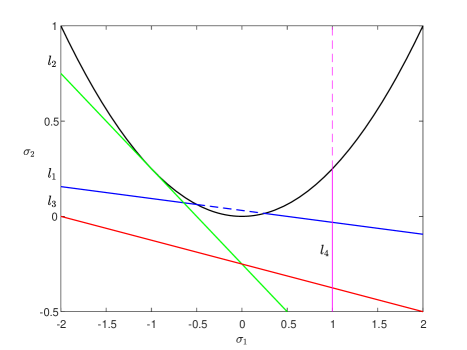
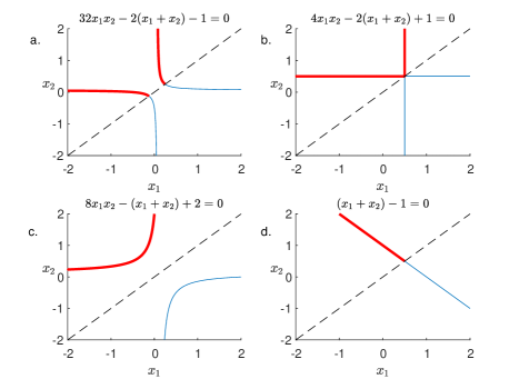
Figure 1: Typical projections of Prony curves.

In order to determine for which points $\mu=(\mu_{0},\mu_{1},\mu_{2},\mu_{3},\mu_{4})$ there is a collision of nodes observe that in terms of the symmetric polynomials $\sigma_{1},\sigma_{2}$ and $\sigma_{3}$ the nodes $x_{1}$ and $x_{2}$ collide if and only if the polynomial

$$\hskip-85.35826ptQ(z)=(z-x_{1})(z-x_{2})(z-x_{3})=z^{3}+\sigma_{1}z^{2}+\sigma_{2}z+\sigma_{3}$$

has a double real root which occurs if and only if its discriminant

$$\hskip-93.89418pt\triangle(\sigma_{1},\sigma_{2},\sigma_{3})=27\sigma_{3}^{2}+4\sigma_{2}^{3}-\sigma_{1}^{2}\sigma_{2}^{2}+4\sigma_{1}^{3}\sigma_{3}-18\sigma_{1}\sigma_{2}\sigma_{3}$$

vanishes. In terms of the symmetric polynomials $\sigma_{1},\sigma_{2},\sigma_{3}$ it follows, from equation (4.3), that a collision of nodes occurs if and only if the line

$$\hskip-227.62204pt\mu_{0}\sigma_{3}+\mu_{1}\sigma_{2}+\mu_{2}\sigma_{1}=-\mu_{3},$$

(4.4)

$$\hskip-227.62204pt\mu_{1}\sigma_{3}+\mu_{2}\sigma_{2}+\mu_{3}\sigma_{1}=-\mu_{4}$$

intersects the surface $\triangle(\sigma_{1},\sigma_{2},\sigma_{3})=0$. Using Proposition 1.2 for the special case where $d=3$ it follows that the line (4.4) has the following parametrization

$$\sigma_{1}=\frac{1}{|\mathcal{M}|}\left|\begin{array}[]{ccc}\mu_{0}&\mu_{1}&\mu_{3}\\ \mu_{1}&\mu_{2}&\mu_{4}\\ \mu_{2}&\mu_{3}&-t\end{array}\right|,\sigma_{2}=\frac{1}{|\mathcal{M}|}\left|\begin{array}[]{ccc}\mu_{0}&\mu_{3}&\mu_{2}\\ \mu_{1}&\mu_{4}&\mu_{3}\\ \mu_{2}&-t&\mu_{4}\end{array}\right|,\sigma_{3}=\frac{1}{|\mathcal{M}|}\left|\begin{array}[]{ccc}\mu_{3}&\mu_{1}&\mu_{2}\\ \mu_{4}&\mu_{2}&\mu_{3}\\ -t&\mu_{3}&\mu_{4}\end{array}\right|$$

where $t\in A_{\mu}$. Inserting the above expressions for the variables $\sigma_{1},\sigma_{2}$ and $\sigma_{3}$ into the equation $\triangle(\sigma_{1},\sigma_{2},\sigma_{3})=0$ we obtain an equation of the form

$$\hskip-42.67912ptP_{\mu}(t)=P_{8}(\mu)t^{4}+P_{9}(\mu)t^{3}+P_{10}(\mu)t^{2}+P_{11}(\mu)t+P_{12}(\mu)=0$$ (4.5)

where $P_{k}$ is a homogenous polynomial in the variable $\mu$ of degree $k$. Since equation (4.5) is the restriction of the discriminant $\triangle(\sigma_{1},\sigma_{2},\sigma_{3})$ to the line (4.4) it follows that for every root $t_{0}$ to equation (4.5) at least two nodes from $x_{1}(t_{0}),x_{2}(t_{0})$ or $x_{3}(t_{0})$ coincide and this in particular implies that all these nodes are real at $t=t_{0}$. Since the set $A_{\mu}$ consists of all $t\in\mathbb{R}$ such that all the nodes $x_{1},x_{2}$ and $x_{3}$ are real and distinct it follows that $t_{0}$ is a boundary point of $A_{\mu}$. Thus, the condition that $t\in A_{\mu}$ does not restrict the inclusion of any of the roots of equation (4.5) when considering nodes collision.

Thus, a collision of nodes occurs if and only if the polynomial $P_{\mu}$ in the left hand side of equation (4.5) has at least one real root. This answers Question A for $d=3$.

Contrary to the case $d=2$, for the case $d=3$ we preferred not to give an explicit relation on the parameters $\mu_{0},...,\mu_{4}$ for determining when collision of nodes occurs (or equivalently when $P_{\mu}$ has at least one real root) since this relation turns out to be overly complicated. One would hope that this relation could be written in a more compact form by expressing it in terms of the determinant of the matrix $\mathcal{M}$ and its minors.

Our aim now is to determine for which points $\mu=(\mu_{0},\mu_{1},\mu_{2},\mu_{3},\mu_{4})$ the projection $S_{4}^{X}(\mu)$ is bounded. Observe that in terms of the symmetric polynomials $\sigma_{1},\sigma_{2}$ and $\sigma_{3}$ each point $x$ in $S_{4}^{X}(\mu)$ corresponds, by the Vieta mapping, to a point $(\sigma_{1},\sigma_{2},\sigma_{3})$ on the line (4.4) for which $\triangle(\sigma_{1},\sigma_{2},\sigma_{3})<0$ (the last condition on the discriminant guarantees that all the roots of $Q$ all real and distinct). By a direct computation we obtain that

$$\hskip-65.44142ptP_{8}(\mu)=4\left|\begin{array}[]{cc}\mu_{0}&\mu_{1}\\ \mu_{1}&\mu_{2}\end{array}\right|^{3}\left|\begin{array}[]{cc}\mu_{1}&\mu_{2}\\ \mu_{2}&\mu_{3}\end{array}\right|-\left|\begin{array}[]{cc}\mu_{0}&\mu_{1}\\ \mu_{1}&\mu_{2}\end{array}\right|^{2}\left|\begin{array}[]{cc}\mu_{0}&\mu_{2}\\ \mu_{1}&\mu_{3}\end{array}\right|^{2}$$

$$\hskip-93.89418pt=-\frac{\mu_{0}^{4}}{27}\left|\begin{array}[]{cc}\mu_{0}&\mu_{1}\\ \mu_{1}&\mu_{2}\end{array}\right|^{2}\triangle\left(\frac{3\mu_{1}}{\mu_{0}},\frac{3\mu_{2}}{\mu_{0}},\frac{\mu_{3}}{\mu_{0}}\right).$$

Hence, if

$$\hskip-236.15796pt\mu_{0}\neq 0,\left|\begin{array}[]{cc}\mu_{0}&\mu_{1}\\ \mu_{1}&\mu_{2}\end{array}\right|\neq 0$$ (4.6)

then $S_{4}^{X}(\mu)$ is bounded in case where

$$\hskip-142.26378ptK(\mu_{0},\mu_{1},\mu_{2},\mu_{3}):=\triangle\left(\frac{3\mu_{1}}{\mu_{0}},\frac{3\mu_{2}}{\mu_{0}},\frac{\mu_{3}}{\mu_{0}}\right)<0$$ (4.7)

and unbounded if $K(\mu_{0},\mu_{1},\mu_{2},\mu_{3})>0$. Indeed, if (4.7) holds then the polynomial $P_{\mu}$ will be nonpositive only inside a bounded interval $I$ in the variable $t$. The polynomial $P_{\mu}$ is the discriminant of the polynomial $Q$ restricted to the line defined by the system of equations (4.4). Hence, $\triangle(\sigma_{1}(t),\sigma_{2}(t),\sigma_{3}(t))\leq 0$ only for $t\in I$ and since all the roots of $Q$ are real if and only if $\triangle(\sigma_{1},\sigma_{2},\sigma_{3})\leq 0$ it follows that our parametrization, in the variable $t$, for the variables $\sigma_{1},\sigma_{2}$ and $\sigma_{3}$ will be inside the interval $I$. That is, the set $A_{\mu}$ which parameterizes the symmetric polynomials $\sigma_{1},\sigma_{2}$ and $\sigma_{3}$ satisfies $A_{\mu}\subseteq I$ where $I$ is bounded. This implies in particular that $\sigma_{1},\sigma_{2}$ and $\sigma_{3}$ are bounded and thus, from the definition of the Vieta mapping, the nodes $x_{1},x_{2}$ and $x_{3}$ in the projection $S_{4}^{X}(\mu)$ will also be bounded.

In the exact same way we can show that if $K(\mu_{0},\mu_{1},\mu_{2},\mu_{3})>0$ then $S_{4}^{X}(\mu)$ is unbounded. This answers Question B for the case $d=3$ in the general case when $P_{8}(\mu)\neq 0$. In the extreme case where $P_{8}(\mu)=0$ then we can make the exact same analysis on the coefficients $P_{9},...,P_{12}$ that are left in order to determine whether $S_{4}^{X}(\mu)$ is bounded or not. The details are left for the reader.

5 Appendix

Proof of Lemma 1.1: For a fixed vector $\mu=(\mu_{0},...,\mu_{q})\in\mathbb{R}^{q+1}$ our aim is to show that the projection $X$ of each point $(A,X)\in\mathcal{P}_{d}$, satisfying the system (1.3), to the nodes parameter space $\mathcal{P}_{d}^{X}$ satisfies the system (1.5) and vice versa that each point $X\in\mathcal{P}_{d}^{X}\subset\mathbb{R}^{d}$, satisfying the system (1.5), also satisfies the system (1.3) for some point $A=(a_{1},...,a_{d})\in\mathcal{P}_{d}^{A}$.

For the proof of the first direction let us take the projection $X$ to the nodes parameter space $\mathcal{P}_{d}^{X}$ of a point $(A,X)\in\mathcal{P}_{d}$ which satisfies the system (1.3). For each $z\in\mathbb{C}$ the symmetric polynomials $\sigma_{1},...,\sigma_{d}$ satisfy

$$\hskip-56.9055ptQ(z)=(z-x_{1})(z-x_{2})...(z-x_{d})=z^{d}+\sigma_{1}(X)z^{d-1}+...+\sigma_{d}(X).$$ (5.1)

Hence, it follows that for $d\leq l\leq q$ we have

$$\hskip-99.58464pt\sum_{i=0}^{d}\mu_{l-i}\sigma_{i}(X)=\sum_{i=0}^{d}\sigma_{i}(X)\sum_{j=1}^{d}a_{j}x_{j}^{l-i}=\sum_{j=1}^{d}a_{j}\sum_{i=0}^{d}\sigma_{i}(X)x_{j}^{l-i}$$

$$\hskip-136.5733pt=\sum_{j=1}^{d}a_{j}x_{j}^{l-d}\sum_{i=0}^{d}\sigma_{i}(X)x_{j}^{d-i}=\sum_{j=1}^{d}a_{j}x_{j}^{l-d}Q(x_{j})=0$$

where in the notation $\sigma_{0}$ we mean that $\sigma_{0}=1$ and where in the last passage we used the fact that the polynomial $Q$ vanishes at the points $x_{i},i=1,...,d$ as can be seen from equation (5.1). This proves the first direction in the proof of Lemma 1.1.

For the proof of the opposite direction, assume that $X\in\mathcal{P}_{d}^{X}$ satisfies equation (1.5), then we need to find a point $(A,Y)\in\mathcal{P}_{d}$ which satisfies the system (1.3) and such that its projection to the nodes parameter space $\mathcal{P}_{d}^{X}$ coincides with $X$, i.e., $Y=X$. Observe that by our assumption that $q\geq d$ it follows that for every point $(A,Y)\in\mathcal{P}_{d}$ which satisfies the system (1.3) the point $A$ is uniquely determined by the first $d$ equations of (1.3) which is a nondegenerate system of equations of Vandermonde’s type since $Y\in\mathcal{P}_{d}^{X}$. Hence, we only need to show that by choosing $Y=X$ the last $q-d+1$ equations of the system (1.3) are satisfied assuming that the first $d$ equations of (1.3) are satisfied and that $X$ is a solution to (1.5). First we will prove that if the first $d+k-1$ equations of the system (1.3) are satisfied where $1\leq k\leq q-d+1$ and $X$ satisfies the system (1.5) then the $(d+k)^{th}$ equation of the system (1.3) is satisfied. Since the first $d+k-1$ equations in the system (1.3) are satisfied it follows in particular that the quantities $\mu_{k-1},...,\mu_{k+d-2}$ can be expressed by the moments of the point $X$. Thus, from the $k^{th}$ equation of the system (1.5) we have

$$\hskip-85.35826pt\mu_{d+k-1}=-\sum_{i=1}^{d}\mu_{k+d-i-1}\varrho_{i}(X)=-\sum_{i=1}^{d}\sum_{j=1}^{d}a_{j}x_{j}^{k+d-i-1}\varrho_{i}(X)$$

$$\hskip-14.22636pt=-\sum_{j=1}^{d}\sum_{i=1}^{d}a_{j}x_{j}^{k+d-i-1}\varrho_{i}(X)=-\sum_{j=1}^{d}a_{j}x_{j}^{k-1}\left(Q(x_{j})-x_{j}^{d}\right)=\sum_{j=1}^{d}a_{j}x_{j}^{d+k-1}$$

where in the fourth and fifth passages we used equation (5.1). Hence, we proved that the $(d+k)^{th}$ equation of the system (1.3) is satisfied. Now the opposite direction follows easily by induction. Indeed, Since by our assumption the first $d$ equations in (1.3) are satisfied then it follows that the $(d+1)^{th}$ equation is satisfied. Assume now that the first $d+m$ equations in the system (1.3) are satisfied where $0\leq m\leq q-d$, then in particular the last $d$ equations in this family of equations are satisfied and thus the $(d+m+1)^{th}$ equation is satisfied. This finishes the proof by induction and thus the system of equations (1.3) is satisfied. Hence, Lemma 1.1 is proved.

References

[1] A.A. Akinshin, D. Batenkov, G. Goldman and Y. Yomdin. Error amplification in solving Prony system with near-colliding nodes, preprint, arXiv:1701.04058.
[2] A.A. Akinshin, D. Batenkov and Y. Yomdin. Accuracy of spike-train Fourier reconstruction for colliding nodes in Sampling Theory and Applications (SampTA), pp. 617-621 (IEEE, 2015).
[3] A.A.Akinshin, G. Goldman, V.P. Golubyatnikov and Y. Yomdin. Accuracy
of reconstruction of spike-trains with two near-colliding nodes, to appear,
arXiv:1701.01482.
[4] A.A. Akinshin, V.P. Golubyatnikov and Y. Yomdin. Low-dimensional Prony
systems (In Russian), Proc. International Conference ”Lomonosov readings
in Altai: fundamental problems of science and education”, Barnaul, Altai state university. pp. 443-450, 20-24 October 2015.
[5] J. Auton. Investigation of Procedures for Automatic Resonance Extrac-
tion from Noisy Transient Electromagnetics Data. Volume III. Translation
of Pronyג€™s Original Paper and Bibliography of Pronyג€™s Method,
Tech. rep., Effects Technology, Santa Barbara, CA, 1981.
[6] J. M. Azaïs, Y. De Castro and F. Gamboa. Spike detection
from inaccurate samplings, Appl. Comput. Harmon. Anal. 38, no.
2, 177195, 2015.
[7] D. Batenkov. Accurate solution of near-colliding Prony systems via decimation and homotopy continuation, Theoretical Computer
Science, Vol. 681, pp 27-40, June 2017.
[8] D. Batenkov. Stability and super-resolution of generalized
spike recovery, Applied and Computational Harmonic Analysis,
Available online 5 October 2016, ISSN 1063-5203,
[9] D. Batenkov and Y. Yomdin. On the accuracy of solving confluent Prony
systems, SIAM J.Appl.Math., 73(1):134-154, 2013.
[10] E. Bernard, J. Odendaal and C. W. I. Pistorius. Two-dimensional superresolution radar imaging using the MUSIC algorithm, IEEE Transactions on Antennas and Propagation, 42(10):1386-1391, 1994.
[11] G. Beylkin and L. Monzon. Approximation by exponential sums revisited,
Appl. Comput. Harmon. Anal. 28, 131-149, 2010.
[12] E. J. Candès and C. Fernandez-Granda. Super-Resolution
from Noisy Data, Journal of Fourier Analysis and Applications,
19(6):1229-1254, December 2013.
[13] E. J. Candès and C. Fernandez-Granda. Towards a Mathematical Theory of Super-resolution, Communications on Pure and Applied
Mathematics, 67(6):906-956, June 2014.
[14] E. J. Candès and V. Morgenshtern. Super-resolution of positive sources: the
discrete setup, SIAM J. Imaging Sci. 9, no. 1, 412-444, 2016.
[15] L. Demanet, D. Needell and N. Nguyen. Super-resolution
via superset selection and pruning, In Proceedings of the 10th International
Conference on Sampling Theory and Applications (SAMPTA),
2013.
[16] L. Demanet and N. Nguyen. The recoverability limit for superresolution
via sparsity, Preprint, 2014. arXiv:1502.01385.
[17] D.L. Donoho. Superresolution via sparsity constraints, SIAM Journal on
Mathematical Analysis, 23(5):1309-1331, 1992.
[18] C. Fernandez-Granda. Super-resolution of point sources via convex programming, Inf. Inference 5, no. 3, 2016.
[19] P. K. Fullagar and S. Levy. Reconstruction of a sparse spike train from a portion of its spectrum and application to highג€ resolution deconvolution. Geophysics, 46(9), 1235-1243, 1981.
[20] S. Kawate, K. Minami and S. Minami. Superresolution of Fourier transform spectra by autoregressive model fitting with singular value decomposition, Appl. Optics, 24: 162-167, 1985.
[21] C. W. McCutchen. Superresolution in Microscopy and the Abbe Resolution Limit, J. Opt. Soc. Am., 57(10):1190-1192, 1967.
[22] T. Peter and G. Plonka. A generalized Prony method for reconstruction of
sparse sums of eigenfunctions of linear operators, Inverse Problems 29, 025001, 2013.
[23] T. Peter, D. Potts, and M. Tasche. Nonlinear approximation by sums
of exponentials and translates. SIAM Journal on Scientific Computing,
33(4), 1920-1947, 2011.
[24] G. Plonka and M. Wischerhoff. How many Fourier samples are needed
for real function reconstruction?, J. Appl. Math. Comput. 42, 117-137,
2013.
[25] D. Potts and M. Tasche. Fast ESPRIT algorithms based on
partial singular value decompositions, Appl. Numer. Math. 88, 31-45, 2015.
[26] R. Prony. Essai experimental et analytique, J. Ec. Polytech. (Paris), 2, pp. 24-76, 1795.
[27] L. R. Turner. Inverse of the Vandermonde matrix with applications, NASA technical
note, D-3547, Aug 1966.