Variance-Aware Regret Bounds for Undiscounted Reinforcement Learning in MDPs

\nameMohammad Sadegh Talebi \emailmstms@kth.se
\addrKTH Royal Institute of Technology, Stockholm, Sweden \AND\nameOdalric-Ambrym Maillard \emailodalric.maillard@inria.fr
\addrINRIA Lille โ€“ Nord Europe, Villeneuve dโ€™Ascq, France
The authors contributed equally.The authors contributed equally.
Abstract

The problem of reinforcement learning in an unknown and discrete Markov Decision Process (MDP) under the average-reward criterion is considered, when the learner interacts with the system in a single stream of observations, starting from an initial state without any reset. We revisit the minimax lower bound for that problem by making appear the local variance of the bias function in place of the diameter of the MDP. Furthermore, we provide a novel analysis of the KL-Ucrlย algorithm establishing a high-probability regret bound scaling as ๐’ช~โ€‹(Sโ€‹โˆ‘s,a๐•s,aโ‹†โ€‹T)~๐’ช๐‘†subscript๐‘ ๐‘Žsubscriptsuperscript๐•โ‹†๐‘ ๐‘Ž๐‘‡\widetilde{{\mathcal{O}}}\Bigl{(}{\textstyle\sqrt{S\sum_{s,a}{\bf V}^{\star}_{s,a}T}}\Big{)} for this algorithm for ergodic MDPs, where $S$ denotes the number of states and where ๐•s,aโ‹†subscriptsuperscript๐•โ‹†๐‘ ๐‘Ž{\bf V}^{\star}_{s,a} is the variance of the bias function with respect to the next-state distribution following action $a$ in state s๐‘ s. The resulting bound improves upon the best previously known regret bound $\widetilde{{\mathcal{O}}}(DS\sqrt{AT})$ for that algorithm, where $A$ and $D$ respectively denote the maximum number of actions (per state) and the diameter of MDP. We finally compare the leading terms of the two bounds in some benchmark MDPs indicating that the derived bound can provide an order of magnitude improvement in some cases. Our analysis leverages novel variations of the transportation lemma combined with Kullback-Leibler concentration inequalities, that we believe to be of independent interest.

Keywords: Undiscounted Reinforcement Learning, Markov Decision Processes, Concentration Inequalities, Regret Minimization, Bellman Optimality

1 Introduction

In this paper, we consider Reinforcement Learning (RL) in an unknown and discrete Markov Decision Process (MDP) under the average-reward criterion, when the learner interacts with the system in a single stream of observations, starting from an initial state without any reset. More formally, let $M=({\mathcal{S}},{\mathcal{A}},\nu,P)$ denote an MDP where ${\mathcal{S}}$ is a finite set of states and ${\mathcal{A}}$ is a finite set of actions available at any state, with respective cardinalities $S$ and $A$. The reward function and the transition kernel is respectively denoted by $\nu$ and $P$. The game goes as follows: the learner starts in some state s1โˆˆ๐’ฎsubscript๐‘ 1๐’ฎs_{1}\in\mathcal{S} at time $t=1$. At each time step $t\in\mathbb{N}$, the learner chooses one action $a\in\mathcal{A}$ in her current state sโˆˆ๐’ฎ๐‘ ๐’ฎs\in\mathcal{S} based on her past decisions and observations. When executing action $a$ in state s๐‘ s, the learner receives a random reward $r$ drawn independently from distribution ฮฝโ€‹(s,a)๐œˆ๐‘ ๐‘Ž\nu(s,a) with support $[0,1]$ and mean ฮผโ€‹(s,a)๐œ‡๐‘ ๐‘Ž\mu(s,a). The state then transits to a next state sโ€ฒโˆˆ๐’ฎsuperscript๐‘ โ€ฒ๐’ฎs^{\prime}\in{\mathcal{S}} sampled with probability pโ€‹(sโ€ฒ|s,a)๐‘conditionalsuperscript๐‘ โ€ฒ๐‘ ๐‘Žp(s^{\prime}|s,a), and a new decision step begins. As the transition probabilities and reward functions are unknown, the learner has to learn them by trying different actions and recording the realized rewards and state transitions. We refer to standard textbooks (Sutton and Barto, 1998; Puterman, 2014) for background material on RL and MDPs.

The performance of the learner can be quantified through the notion of regret, which compares the reward collected by the learner (or the algorithm) to that obtained by an oracle always following an optimal policy, where a policy is a mapping from states to actions. More formally, let $\pi:\mathcal{S}\to\mathcal{P}(\mathcal{A})$ denote a possibly stochastic policy. We further introduce the notation pโ€‹(sโ€ฒ|s,ฯ€โ€‹(s))=๐”ผZโˆผฯ€โ€‹(s)โ€‹[pโ€‹(sโ€ฒ|s,Z)]๐‘conditionalsuperscript๐‘ โ€ฒ๐‘ ๐œ‹๐‘ subscript๐”ผsimilar-to๐‘๐œ‹๐‘ delimited-[]๐‘conditionalsuperscript๐‘ โ€ฒ๐‘ ๐‘p(s^{\prime}|s,\pi(s))=\mathbb{E}_{Z\sim\pi(s)}[p(s^{\prime}|s,Z)], and $P_{\pi}f$ to denote the function sโ†ฆโˆ‘sโ€ฒโˆˆ๐’ฎpโ€‹(sโ€ฒ|s,ฯ€โ€‹(s))โ€‹fโ€‹(sโ€ฒ)maps-to๐‘ subscriptsuperscript๐‘ โ€ฒ๐’ฎ๐‘conditionalsuperscript๐‘ โ€ฒ๐‘ ๐œ‹๐‘ ๐‘“superscript๐‘ โ€ฒs\mapsto\sum_{s^{\prime}\in\mathcal{S}}p(s^{\prime}|s,\pi(s))f(s^{\prime}). Likewise, let ฮผฯ€โ€‹(s)=๐”ผZโˆผฯ€โ€‹(s)โ€‹[ฮผโ€‹(s,Z)]subscript๐œ‡๐œ‹๐‘ subscript๐”ผsimilar-to๐‘๐œ‹๐‘ delimited-[]๐œ‡๐‘ ๐‘\mu_{\pi}(s)=\mathbb{E}_{Z\sim\pi(s)}[\mu(s,Z)] denote the mean reward after choosing action ฯ€โ€‹(s)๐œ‹๐‘ \pi(s) in step s๐‘ s.

Definition 1 (Expected cumulative reward)

The expected cumulative reward of policy $\pi$ when run for $T$ steps from initial state s1subscript๐‘ 1s_{1} is defined as

Rฯ€,Tโ€‹(s1)=๐”ผโ€‹[โˆ‘t=1Trโ€‹(st,at)]=ฮผฯ€โ€‹(s1)+(Pฯ€โ€‹ฮผฯ€)โ€‹(s1)+โ‹ฏ=โˆ‘t=1T(Pฯ€tโˆ’1โ€‹ฮผฯ€)โ€‹(s1).subscript๐‘…๐œ‹๐‘‡subscript๐‘ 1๐”ผdelimited-[]superscriptsubscript๐‘ก1๐‘‡๐‘Ÿsubscript๐‘ ๐‘กsubscript๐‘Ž๐‘กsubscript๐œ‡๐œ‹subscript๐‘ 1subscript๐‘ƒ๐œ‹subscript๐œ‡๐œ‹subscript๐‘ 1โ‹ฏsuperscriptsubscript๐‘ก1๐‘‡superscriptsubscript๐‘ƒ๐œ‹๐‘ก1subscript๐œ‡๐œ‹subscript๐‘ 1\displaystyle R_{\pi,T}(s_{1})=\mathbb{E}\bigg{[}\sum_{t=1}^{T}r(s_{t},a_{t})\bigg{]}=\mu_{\pi}(s_{1})+(P_{\pi}\mu_{\pi})(s_{1})+\dots=\sum_{t=1}^{T}(P_{\pi}^{t-1}\mu_{\pi})(s_{1})\,.

where atโˆผฯ€โ€‹(st)similar-tosubscript๐‘Ž๐‘ก๐œ‹subscript๐‘ ๐‘กa_{t}\sim\pi(s_{t}), $s_{t+1}\sim p(\cdot|s_{t},a_{t})$, and finally rโ€‹(s,a)โˆผฮฝโ€‹(s,a)similar-to๐‘Ÿ๐‘ ๐‘Ž๐œˆ๐‘ ๐‘Žr(s,a)\sim\nu(s,a).

Definition 2 (Average gain and bias)

Let us introduce the average transition operator $\overline{P}_{\pi}=\lim_{T\to\infty}\frac{1}{T}\sum_{t=1}^{T}P_{\pi}^{t-1}$. The average gain $g_{\pi}$ and bias function $b_{\pi}$ are defined by

gฯ€โ€‹(s1)=limTโ†’โˆž1Tโ€‹Rฯ€,Tโ€‹(s1)=(Pยฏฯ€โ€‹ฮผฯ€)โ€‹(s1),bฯ€โ€‹(s)=โˆ‘t=1โˆž((Pฯ€tโˆ’1โˆ’Pยฏฯ€)โ€‹ฮผฯ€)โ€‹(s).formulae-sequencesubscript๐‘”๐œ‹subscript๐‘ 1subscriptโ†’๐‘‡1๐‘‡subscript๐‘…๐œ‹๐‘‡subscript๐‘ 1subscriptยฏ๐‘ƒ๐œ‹subscript๐œ‡๐œ‹subscript๐‘ 1subscript๐‘๐œ‹๐‘ superscriptsubscript๐‘ก1superscriptsubscript๐‘ƒ๐œ‹๐‘ก1subscriptยฏ๐‘ƒ๐œ‹subscript๐œ‡๐œ‹๐‘ \displaystyle g_{\pi}(s_{1})=\lim_{T\to\infty}\frac{1}{T}R_{\pi,T}(s_{1})=(\overline{P}_{\pi}\mu_{\pi})(s_{1})\,,\qquad b_{\pi}(s)=\sum_{t=1}^{\infty}\Big{(}(P_{\pi}^{t-1}-\overline{P}_{\pi})\mu_{\pi}\Big{)}(s)\,.

The previous definition requires some mild assumption on the MDP for the limits to makes sense. It is shown (see, e.g., (Puterman, 2014)) that the average gain achieved by executing a stationary policy $\pi$ in a communicating MDP $M$ is well-defined and further does not depend on the initial state, i.e., gฯ€โ€‹(s1)=gฯ€subscript๐‘”๐œ‹subscript๐‘ 1subscript๐‘”๐œ‹g_{\pi}(s_{1})=g_{\pi}. For this reason, we restrict our attention to such MDPs in the rest of this paper. Furthermore, let $\star$ denote an optimal policy, that is111The maximum is reached since there are only finitely many deterministic policies. $g_{\star}=\max_{\pi}g_{\pi}.$

Definition 3 (Regret)

We define the regret of any learning algorithm $\mathbb{A}$ after $T$ steps as

$\displaystyle\mathrm{Regret}_{\mathbb{A},T}:=\sum_{t=1}^{T}r(s_{t}^{\star},\star(s_{t}^{\star}))-\sum_{t=1}^{T}r(s_{t},a_{t})\quad\text{where }a_{t}=\mathbb{A}(s_{t},(\{s_{t^{\prime}},a_{t^{\prime}},r_{t^{\prime}}\})_{t^{\prime}<t})\,,$

and $s^{\star}_{t+1}\sim p(\cdot|s^{\star}_{t},\star(s^{\star}_{t}))$ with s1โ‹†=s1subscriptsuperscript๐‘ โ‹†1subscript๐‘ 1s^{\star}_{1}=s_{1} is a sequence generated by the optimal strategy.

By an application of Azuma-Hoeffdingโ€™s inequality for bounded random martingales, it is immediate to show that with probability higher than $1-\delta$,

$\displaystyle\mathrm{Regret}_{\mathbb{A},T}$ $\displaystyle\leqslant$ $\displaystyle\sum_{t=1}^{T}\Big{(}P_{\star}^{t-1}\mu_{\star}-P_{a_{t}}^{t-1}\mu_{a_{t}}\Big{)}+\sqrt{2T\log(2/\delta)}$
$\displaystyle=$ $\displaystyle\sum_{t=1}^{T}(P_{\star}^{t-1}-\overline{P}_{\star})\mu_{\star}+\bigg{[}Tg_{\star}-\sum_{t=1}^{T}P_{a_{t}}^{t-1}\mu_{a_{t}}\bigg{]}+\sqrt{2T\log(2/\delta)}\,.$

Thus, following (Jaksch etย al., 2010), it makes sense to focus on the control of the middle term in brackets only. This leads us to consider the following notion of regret, which we may call effective regret:

โ„œ๐”ธ,T:=Tโ€‹gโ‹†โˆ’โˆ‘t=1Trโ€‹(st,at).assignsubscriptโ„œ๐”ธ๐‘‡๐‘‡superscript๐‘”โ‹†superscriptsubscript๐‘ก1๐‘‡๐‘Ÿsubscript๐‘ ๐‘กsubscript๐‘Ž๐‘ก\displaystyle\mathfrak{R}_{\mathbb{A},T}:=Tg^{\star}-\sum_{t=1}^{T}r(s_{t},a_{t})\,.

To date, several algorithms have been proposed in order to minimize the regret based on the optimism in the face of uncertainty principle, coming from the literature on stochastic multi-armed bandits (see (Robbins, 1952)). Algorithms designed based on this principle typically maintain confidence bounds on the unknown reward and transition distributions, and choose an optimistic model that leads to the highest average long-term reward. One of the first algorithms based on this principle for MDPs is due to (Burnetas and Katehakis, 1997), which is shown to be asymptotically optimal. Their proposed algorithm uses the Kullback-Leibler (KL) divergence to define confidence bounds for transition probabilities. Subsequent studies by (Tewari and Bartlett, 2008), (Auer and Ortner, 2007), (Jaksch etย al., 2010), and (Bartlett and Tewari, 2009) propose algorithms that maintain confidence bounds on transition kernel defined by $L_{1}$ or total variation norm. The use of $L_{1}$ norm, instead of KL-divergence, allows one to describe the uncertainty of the transition kernel by a polytope, which in turn brings computational advantages and ease in the regret analysis. On the other hand, such polytopic models are typically known to provide poor representations of underlying uncertainties; we refer to the literature on the robust control of MDPs with uncertain transition kernels, e.g., (Nilim and Elย Ghaoui, 2005), and more appropriately to (Filippi etย al., 2010). Indeed, as argued in (Filippi etย al., 2010), optimistic models designed by $L_{1}$ norm suffer from two shortcomings: (i) the $L_{1}$ optimistic model could lead to inconsistent models by assigning a zero mass to an already observed element, and (ii) due to polytopic shape of $L_{1}$-induced confidence bounds, the maximizer of a linear optimization over $L_{1}$ ball could significantly vary for a small change in the value function, thus resulting in sub-optimal exploration (we refer to the discussion and illustrations on pages 120โ€“121 in (Filippi etย al., 2010)).

Both of these shortcomings are avoided by making use of the KL-divergence and properties of the corresponding KL-ball. In (Filippi etย al., 2010), the authors introduce the KL-Ucrlย algorithm that modifies the Ucrl2 algorithm of (Jaksch etย al., 2010) by replacing $L_{1}$ norms with KL divergences in order to define the confidence bound on transition probabilities. Further, they provide an efficient way to carry out linear optimization over the KL-ball, which is necessary in each iteration of the Extended Value Iteration. Despite these favorable properties and the strictly superior performance in numerical experiments (even for very short time horizons), the best known regret bound for KL-Ucrlย matches that of Ucrl2. Hence, from a theoretical perspective, the potential gain of use of KL-divergence to define confidence bounds for transition function has remained largely unexplored. The goal of this paper is to investigate this gap.

Main contributions.

In this paper we provide a new regret bound for KL-Ucrlย scaling as ๐’ช~โ€‹(Sโ€‹โˆ‘s,a๐•s,aโ‹†โ€‹T+Dโ€‹T)~๐’ช๐‘†subscript๐‘ ๐‘Žsuperscriptsubscript๐•๐‘ ๐‘Žโ‹†๐‘‡๐ท๐‘‡\widetilde{\mathcal{O}}\bigl{(}\sqrt{S\sum_{s,a}\mathbf{V}_{s,a}^{\star}T}+D\sqrt{T}\big{)} for ergodic MDPs with $S$ states, $A$ actions, and diameter $D$. Here, $\mathbf{V}^{\star}_{s,a}:=\mathbb{V}_{p(\cdot|s,a)}(b^{\star})$ denotes the variance of the optimal bias function $b^{\star}$ of the true (unknown) MDP with respect to next state distribution under state-action (s,a)๐‘ ๐‘Ž(s,a). This bound improves over the best previous bound of $\widetilde{\mathcal{O}}(DS\sqrt{AT})$ for KL-Ucrlย as ๐•s,aโ‹†โฉฝDsuperscriptsubscript๐•๐‘ ๐‘Žโ‹†๐ท\sqrt{\mathbf{V}_{s,a}^{\star}}\leqslant D. Interestingly, in several examples ๐•s,aโ‹†โ‰ชDmuch-less-thansuperscriptsubscript๐•๐‘ ๐‘Žโ‹†๐ท\sqrt{\mathbf{V}_{s,a}^{\star}}\ll D and actually ๐•s,aโ‹†subscriptsuperscript๐•โ‹†๐‘ ๐‘Ž\sqrt{\mathbf{V}^{\star}_{s,a}} is comparable to $\sqrt{D}$. Our numerical experiments on typical MDPs further confirm that Sโ€‹โˆ‘s,a๐•s,aโ‹†๐‘†subscript๐‘ ๐‘Žsuperscriptsubscript๐•๐‘ ๐‘Žโ‹†\sqrt{S\sum_{s,a}\mathbf{V}_{s,a}^{\star}} could be orders of magnitude smaller than $DS\sqrt{A}$. To prove this result, we provide novel transportation concentration inequalities inspired by the transportation method that relate the so-called transportation cost under two discrete probability measures to the KL-divergence between the two measures and the associated variances. To the best of our knowledge, these inequalities are new and of independent interest. To complete our result, we provide a new minimax regret lower bound of order $\Omega(\sqrt{SA\mathbf{V}_{\max}T})$, where ๐•max:=maxs,aโก๐•s,aโ‹†assignsubscript๐•subscript๐‘ ๐‘Žsubscriptsuperscript๐•โ‹†๐‘ ๐‘Ž\mathbf{V}_{\max}:=\max_{s,a}\mathbf{V}^{\star}_{s,a}. In view of the new minimax lower bound, the reported regret bound for KL-Ucrlย can be improved by only a factor $\sqrt{S}$.

Related work.

RL in unknown MDPs under average-reward criterion dates back to the seminal papers by (Graves and Lai, 1997), and (Burnetas and Katehakis, 1997), followed by (Tewari and Bartlett, 2008). Among these studies, for the case of ergodic MDPs, (Burnetas and Katehakis, 1997) derive an asymptotic MDP-dependent lower bound on the regret and provide an asymptotically optimal algorithm. Algorithms with finite-time regret guarantees and for wider class of MDPs are presented by (Auer and Ortner, 2007), (Jaksch etย al., 2010; Auer etย al., 2009), (Bartlett and Tewari, 2009), (Filippi etย al., 2010), and (Maillard etย al., 2014).

Ucrl2ย and KL-Ucrlย achieve a $\widetilde{\mathcal{O}}(DS\sqrt{AT})$ regret bound with high probability in communicating MDPs, for any unknown time horizon. Regal obtains a $\widetilde{\mathcal{O}}(D^{\prime}S\sqrt{AT})$ regret with high probability in the larger class of weakly communicating MDPs, provided that we know an upper bound $D^{\prime}$ on the span of the bias function. It is however still an open problem to incorporate this knowledge into an implementable algorithm. The TSDE algorithm by Ouyang et al.ย (Ouyang etย al., 2017) achieves a regret growing as $\widetilde{\mathcal{O}}(D^{\prime}S\sqrt{AT})$ for the class of weakly communicating MDPs, where $D^{\prime}$ is a given bound on the span of the bias function. In a recent study, (Agrawal and Jia, 2017) propose an algorithm based on posterior sampling for the class of communicating MDPs. Under the assumption of known reward function and known time horizon, their algorithm enjoys a regret bound scaling as $\widetilde{\cal O}(D\sqrt{SAT})$, which constitutes the best known regret upper bound for learning in communicating MDPs and has a tight dependencies on $S$ and $A$.

We finally mention that some studies consider regret minimization in MDPs in the episodic setting, where the length of each episode is fixed and known; see, e.g., (Osband etย al., 2013), (Gheshlaghiย Azar etย al., 2017), and (Dann etย al., 2017). Although RL in the episodic setting bears some similarities to the average-reward setting, the techniques developed in these paper strongly rely on the fixed length of the episode, which is assumed to be small, and do not directly carry over to the case of undiscounted RL considered here.

2 Background Material and The KL-Ucrlย Algorithm

In this section, we recall some basic material on undiscounted MDPs and then detail the KL-Ucrlย algorithm.

Lemma 4 (Bias and Gain)

The gain and bias function satisfy the following relations

$\displaystyle(\text{Bellman equation})\qquad b_{\pi}+g_{\pi}$ $\displaystyle=$ $\displaystyle\mu_{\pi}+P_{\pi}b_{\pi}$
$\displaystyle(\text{Fundamental matrix})\qquad\quad b_{\pi}$ $\displaystyle=$ $\displaystyle[I-P_{\pi}+\overline{P_{\pi}}]^{-1}[I-\overline{P}_{\pi}]\mu_{\pi}\,.$

This result is an easy consequence of the fact that ${\overline{P}}_{\pi}$ (see Definitionย 2) satisfies $\overline{P}_{\pi}P_{\pi}=P_{\pi}\overline{P}_{\pi}=\overline{P}_{\pi}\overline{P}_{\pi}=\overline{P}_{\pi}\,$ (see (Puterman, 2014) as well as Appendixย E for details).

According to the standard terminology, we say a policy is $b_{\star}$-improving if it satisfies ฯ€โ€‹(s)=argโกmaxaโˆˆ๐’œโกฮผโ€‹(s,a)+(Paโ€‹bโ‹†)โ€‹(s)๐œ‹๐‘ subscript๐‘Ž๐’œ๐œ‡๐‘ ๐‘Žsubscript๐‘ƒ๐‘Žsubscript๐‘โ‹†๐‘ \pi(s)=\arg\!\max_{a\in\mathcal{A}}\mu(s,a)+(P_{a}b_{\star})(s)โ€‰. Applying the theory of MDPs (see, e.g., (Puterman, 2014)), it can be shown that any $b_{\star}$-improving policy is optimal and thus that we can choose $\star$ to satisfy222The solution to this fixed-point equation is defined only up to an additive constant. Some people tend to use this equation in order to define $b_{\star}$ and $g_{\star}$, but this is a bad habit that we avoid here. the following fundamental identity333Throughout this paper, we may use $g^{\star}$ (resp.ย bโ‹†superscript๐‘โ‹†b^{\star}) and $g_{\star}$ (resp.ย bโ‹†subscript๐‘โ‹†b_{\star}) interchangeably.

(Bellman optimality equation)โˆ€sโˆˆ๐’ฎ,bโ‹†โ€‹(s)+gโ‹†=maxaโˆˆ๐’œโก(ฮผโ€‹(s,a)+โˆ‘yโˆˆ๐’ฎpโ€‹(y|s,a)โ€‹bโ‹†โ€‹(y)).formulae-sequenceBellman optimality equationfor-all๐‘ ๐’ฎsubscript๐‘โ‹†๐‘ subscript๐‘”โ‹†subscript๐‘Ž๐’œ๐œ‡๐‘ ๐‘Žsubscript๐‘ฆ๐’ฎ๐‘conditional๐‘ฆ๐‘ ๐‘Žsubscript๐‘โ‹†๐‘ฆ\displaystyle(\text{Bellman optimality equation})\quad\forall s\in\mathcal{S},\,b_{\star}(s)+g_{\star}=\max_{a\in{\mathcal{A}}}\Bigl{(}\mu(s,a)+\sum_{y\in{\mathcal{S}}}p(y|s,a)b_{\star}(y)\Big{)}\;.

We now recall the definition of diameter and mixing time as we consider only MDPs with finite diameter or mixing time.

Definition 5 (Diameter (Jaksch etย al., 2010))

Let Tฯ€โ€‹(sโ€ฒ|s)subscript๐‘‡๐œ‹conditionalsuperscript๐‘ โ€ฒ๐‘ T_{\pi}(s^{\prime}|s) denote the first hitting time of state sโ€ฒsuperscript๐‘ โ€ฒs^{\prime} when following stationary policy $\pi$ from initial state s๐‘ s. The diameter $D$ of an MDP $M$ is defined as

D:=maxsโ‰ sโ€ฒโกminฯ€โก๐”ผโ€‹[Tฯ€โ€‹(sโ€ฒ|s)].assign๐ทsubscript๐‘ superscript๐‘ โ€ฒsubscript๐œ‹๐”ผdelimited-[]subscript๐‘‡๐œ‹conditionalsuperscript๐‘ โ€ฒ๐‘ D:=\max_{s\neq s^{\prime}}\min_{\pi}\mathbb{E}[T_{\pi}(s^{\prime}|s)].
Definition 6 (Mixing time (Auer and Ortner, 2007))

Let $\mathcal{C}_{\pi}$ denote the Markov chain induced by the policy $\pi$ in an ergodic MDP $M$ and let $T_{\mathcal{C}_{\pi}}$ represent the hitting time of $\mathcal{C}_{\pi}$. The mixing time $T_{M}$ of $M$ is defined as

$\displaystyle T_{M}:=\max_{\pi}T_{\mathcal{C}_{\pi}}\,.$

For convenience, we also introduce, for any function $f$ defined on ${\mathcal{S}}$, its span defined by ๐•Šโ€‹(f):=maxsโˆˆ๐’ฎโกfโ€‹(s)โˆ’minsโˆˆ๐’ฎโกfโ€‹(s)assign๐•Š๐‘“subscript๐‘ ๐’ฎ๐‘“๐‘ subscript๐‘ ๐’ฎ๐‘“๐‘ \mathbb{S}(f):=\max_{s\in{\mathcal{S}}}f(s)-\min_{s\in{\mathcal{S}}}f(s). It actually acts as a semi-norm (see (Puterman, 2014)).

We finally introduce the following quantity that appears in the known problem-dependent lower-bounds on the regret, and plays the analogue of the mean gap in the bandit literature.

Definition 7 (Sub-optimality gap)

The sub-optimality of action $a$ at state s๐‘ s is

ฯ†โ€‹(s,a)๐œ‘๐‘ ๐‘Ž\displaystyle\varphi(s,a) $\displaystyle=\mu(s,\star(s))-\mu(s,a)+(p(\cdot|s,\star(s))-p(\cdot|s,a))^{\top}{b_{\star}}\;.$ (1)

Note importantly that $\varphi$ is defined in terms of the bias $b_{\star}$ of the optimal policy $\star$. Indeed, it can be shown that minimizing the effective regret (in expectation) is essentially equivalent to minimizing the quantity โˆ‘s,aฯ†โ€‹(s,a)โ€‹๐”ผโ€‹[NTโ€‹(s,a)]subscript๐‘ ๐‘Ž๐œ‘๐‘ ๐‘Ž๐”ผdelimited-[]subscript๐‘๐‘‡๐‘ ๐‘Ž\sum_{s,a}\varphi(s,a)\mathbb{E}[N_{T}(s,a)], where NTโ€‹(s,a)subscript๐‘๐‘‡๐‘ ๐‘ŽN_{T}(s,a) is the total number of steps when action $a$ has been played in state s๐‘ s. More precisely, it is not difficult to show (see Appendixย E for completeness) that for any stationary policy $\pi$ and all $t$,

๐”ผโ€‹[โ„œฯ€,t]=โˆ‘s,aฯ†โ€‹(s,a)โ€‹๐”ผโ€‹[Ntโ€‹(s,a)]+((Pฯ€tโˆ’1โˆ’I)โ€‹bโ‹†)โ€‹(s1)โฉฝโˆ‘s,aฯ†โ€‹(s,a)โ€‹๐”ผโ€‹[Ntโ€‹(s,a)]+D.๐”ผdelimited-[]subscriptโ„œ๐œ‹๐‘กsubscript๐‘ ๐‘Ž๐œ‘๐‘ ๐‘Ž๐”ผdelimited-[]subscript๐‘๐‘ก๐‘ ๐‘Žsubscriptsuperscript๐‘ƒ๐‘ก1๐œ‹๐ผsubscript๐‘โ‹†subscript๐‘ 1subscript๐‘ ๐‘Ž๐œ‘๐‘ ๐‘Ž๐”ผdelimited-[]subscript๐‘๐‘ก๐‘ ๐‘Ž๐ท\displaystyle\mathbb{E}[\mathfrak{R}_{\pi,t}]=\sum_{s,a}\varphi(s,a)\mathbb{E}[N_{t}(s,a)]+{\big{(}(P^{t-1}_{\pi}-I)b_{\star}\big{)}(s_{1})}\leqslant\sum_{s,a}\varphi(s,a)\mathbb{E}[N_{t}(s,a)]+D\,. (2)
The KL-Ucrlย algorithm.

The KL-Ucrlย algorithm (Filippi etย al., 2010; Filippi, 2010) is a model-based algorithm inspired by Ucrl2 (Jaksch etย al., 2010). To present the algorithm, we first describe how it defines, at each given time $t$, the set of plausible MDPs based on the observation available at that time. To this end, we introduce the following notations. Under a given algorithm and for a state-action pair (s,a)๐‘ ๐‘Ž(s,a), let Ntโ€‹(s,a)subscript๐‘๐‘ก๐‘ ๐‘ŽN_{t}(s,a) denote the number of visits, up to time $t$, to (s,a)๐‘ ๐‘Ž(s,a): Ntโ€‹(s,a)=โˆ‘tโ€ฒ=0tโˆ’1๐•€โ€‹{stโ€ฒ=s,atโ€ฒ=a}subscript๐‘๐‘ก๐‘ ๐‘Žsuperscriptsubscriptsuperscript๐‘กโ€ฒ0๐‘ก1๐•€formulae-sequencesubscript๐‘ superscript๐‘กโ€ฒ๐‘ subscript๐‘Žsuperscript๐‘กโ€ฒ๐‘ŽN_{t}(s,a)=\sum_{t^{\prime}=0}^{t-1}\mathbb{I}\{s_{t^{\prime}}=s,a_{t^{\prime}}=a\}. Then, let Ntโ€‹(s,a)+=maxโก{Ntโ€‹(s,a),1}subscript๐‘๐‘กsuperscript๐‘ ๐‘Žsubscript๐‘๐‘ก๐‘ ๐‘Ž1N_{t}(s,a)^{+}=\max\{N_{t}(s,a),1\}. Similarly, Ntโ€‹(s,a,sโ€ฒ)subscript๐‘๐‘ก๐‘ ๐‘Žsuperscript๐‘ โ€ฒN_{t}(s,a,s^{\prime}) denotes the number of visits to (s,a)๐‘ ๐‘Ž(s,a), up to time $t$, followed by a visit to state sโ€ฒsuperscript๐‘ โ€ฒs^{\prime}: Ntโ€‹(s,a,sโ€ฒ)=โˆ‘tโ€ฒ=0tโˆ’1๐•€โ€‹{stโ€ฒ=s,atโ€ฒ=a,stโ€ฒ+1=sโ€ฒ}subscript๐‘๐‘ก๐‘ ๐‘Žsuperscript๐‘ โ€ฒsuperscriptsubscriptsuperscript๐‘กโ€ฒ0๐‘ก1๐•€formulae-sequencesubscript๐‘ superscript๐‘กโ€ฒ๐‘ formulae-sequencesubscript๐‘Žsuperscript๐‘กโ€ฒ๐‘Žsubscript๐‘ superscript๐‘กโ€ฒ1superscript๐‘ โ€ฒN_{t}(s,a,s^{\prime})=\sum_{t^{\prime}=0}^{t-1}\mathbb{I}\{s_{t^{\prime}}=s,a_{t^{\prime}}=a,s_{t^{\prime}+1}=s^{\prime}\}. We introduce the empirical estimates of transition probabilities and rewards:

ฮผ^tโ€‹(s,a)=โˆ‘tโ€ฒ=0tโˆ’1rtโ€‹๐•€โ€‹{stโ€ฒ=s,atโ€ฒ=a}Ntโ€‹(s,a)+,p^tโ€‹(sโ€ฒ|s,a)=Ntโ€‹(s,a,sโ€ฒ)Ntโ€‹(s,a)+.formulae-sequencesubscript^๐œ‡๐‘ก๐‘ ๐‘Žsuperscriptsubscriptsuperscript๐‘กโ€ฒ0๐‘ก1subscript๐‘Ÿ๐‘ก๐•€formulae-sequencesubscript๐‘ superscript๐‘กโ€ฒ๐‘ subscript๐‘Žsuperscript๐‘กโ€ฒ๐‘Žsubscript๐‘๐‘กsuperscript๐‘ ๐‘Žsubscript^๐‘๐‘กconditionalsuperscript๐‘ โ€ฒ๐‘ ๐‘Žsubscript๐‘๐‘ก๐‘ ๐‘Žsuperscript๐‘ โ€ฒsubscript๐‘๐‘กsuperscript๐‘ ๐‘Ž\displaystyle\hat{\mu}_{t}(s,a)=\frac{\sum_{t^{\prime}=0}^{t-1}r_{t}\mathbb{I}\{s_{t^{\prime}}=s,a_{t^{\prime}}=a\}}{N_{t}(s,a)^{+}},\quad\hat{p}_{t}(s^{\prime}|s,a)=\frac{N_{t}(s,a,s^{\prime})}{N_{t}(s,a)^{+}}\,.

KL-Ucrl, as an optimistic model-based approach, considers the set ${\mathcal{M}}_{t}$ as a collection of all MDPs $M^{\prime}=({\mathcal{S}},{\mathcal{A}},\nu^{\prime},P^{\prime})$, whose transition kernels and reward functions satisfy:

$\displaystyle\texttt{KL}(\hat{p}_{t}(\cdot|s,a),p^{\prime}(\cdot|s,a))$ $\displaystyle\leqslant$ Cp/Ntโ€‹(s,a),subscript๐ถ๐‘subscript๐‘๐‘ก๐‘ ๐‘Ž\displaystyle C_{p}/N_{t}(s,a)\,, (3)
|ฮผ^tโ€‹(s,a)โˆ’ฮผโ€ฒโ€‹(s,a)|subscript^๐œ‡๐‘ก๐‘ ๐‘Žsuperscript๐œ‡โ€ฒ๐‘ ๐‘Ž\displaystyle|\hat{\mu}_{t}(s,a)-{\mu^{\prime}}(s,a)| $\displaystyle\leqslant$ Cฮผ/Ntโ€‹(s,a),subscript๐ถ๐œ‡subscript๐‘๐‘ก๐‘ ๐‘Ž\displaystyle\sqrt{C_{\mu}/N_{t}(s,a)}\,, (4)

where $\mu^{\prime}$ denotes the mean of $\nu^{\prime}$, and where $C_{p}:=C_{p}(T,\delta)=S\left(B+\log(G)(1+1/G)\right)$, with $B=B(T,\delta):=\log(2eS^{2}A\log(T)/\delta)$ and $G=B+1/\log(T)$, and $C_{\mu}:=C_{\mu}(T,\delta)=\log(4SA\log(T)/\delta)/1.99$. Importantly, as proven in (Filippi etย al., 2010, Propositionย 1), with probability at least $1-2\delta$, the true MDP $M$ belongs to the set ${\mathcal{M}}_{t}$ uniformly over all time steps $t\leqslant T$.

Similarly to Ucrl2, KL-Ucrlย proceeds in episodes of varying lengths; see Algorithmย 1. We index an episode by $k\in{\mathbb{N}}$. The starting time of the $k$-th episode is denoted $t_{k}$, and by a slight abuse of notation, let ${\mathcal{M}}_{k}:={\mathcal{M}}_{t_{k}}$, $N_{k}:=N_{t_{k}}$, $\hat{\mu}_{k}=\hat{\mu}_{t_{k}}$, and $\hat{p}_{k}:=\hat{p}_{t_{k}}$. At $t=t_{k}$, the algorithm forms the set of plausible MDPs ${\mathcal{M}}_{k}$ based on the observations gathered so far. It then defines an extended MDP $M_{\texttt{ext},k}=({\mathcal{S}},{\mathcal{A}}\times\mathcal{M}_{k},\mu_{\texttt{ext}},P_{\texttt{ext}})$, where for an extended action $a_{\texttt{ext}}=(a,M^{\prime})$, it defines ฮผextโ€‹(s,aext)=ฮผโ€ฒโ€‹(s,a)subscript๐œ‡ext๐‘ subscript๐‘Žextsuperscript๐œ‡โ€ฒ๐‘ ๐‘Ž\mu_{\texttt{ext}}(s,a_{\texttt{ext}})=\mu^{\prime}(s,a) and pextโ€‹(sโ€ฒ|s,aext)=pโ€ฒโ€‹(sโ€ฒ|s,a)subscript๐‘extconditionalsuperscript๐‘ โ€ฒ๐‘ subscript๐‘Žextsuperscript๐‘โ€ฒconditionalsuperscript๐‘ โ€ฒ๐‘ ๐‘Žp_{\texttt{ext}}(s^{\prime}|s,a_{\texttt{ext}})=p^{\prime}(s^{\prime}|s,a). Then, a $\frac{1}{\sqrt{t_{k}}}$-optimal extended policy $\pi_{\texttt{ext},k}$ is computed in the form ฯ€ext,kโ€‹(s)=(M~k,ฯ€~kโ€‹(s))subscript๐œ‹ext๐‘˜๐‘ subscript~๐‘€๐‘˜subscript~๐œ‹๐‘˜๐‘ \pi_{\texttt{ext},k}(s)=(\tilde{M}_{k},\tilde{\pi}_{k}(s)), in the sense that it satisfies

$$\tilde{g}_{k}\stackrel{{\scriptstyle\rm def}}{{=}}g_{\tilde{\pi}_{k}}(\tilde{M}_{k})\geqslant\max_{M^{\prime}\in{\mathcal{M}}_{k},\pi}g_{\pi}(M^{\prime})-\frac{1}{\sqrt{t_{k}}}\,,$$

where $g_{\pi}(M)$ denotes the gain of policy $\pi$ in MDP $M$. $\tilde{M}_{k}$ and $\tilde{\pi}_{k}$ are respectively called the optimistic MDP and the optimistic policy. Finally, an episode stops at the first step $t=t_{k+1}$ when the number of local counts vk,tโ€‹(s,a)=โˆ‘tโ€ฒ=tkt๐•€โ€‹{stโ€ฒ=s,atโ€ฒ=a}subscript๐‘ฃ๐‘˜๐‘ก๐‘ ๐‘Žsuperscriptsubscriptsuperscript๐‘กโ€ฒsubscript๐‘ก๐‘˜๐‘ก๐•€formulae-sequencesubscript๐‘ superscript๐‘กโ€ฒ๐‘ subscript๐‘Žsuperscript๐‘กโ€ฒ๐‘Žv_{k,t}(s,a)=\sum_{t^{\prime}=t_{k}}^{t}\mathbb{I}\{s_{t^{\prime}}=s,a_{t^{\prime}}=a\} exceeds Ntkโ€‹(s,a)subscript๐‘subscript๐‘ก๐‘˜๐‘ ๐‘ŽN_{t_{k}}(s,a) for some (s,a)๐‘ ๐‘Ž(s,a). We denote with some abuse $v_{k}=v_{k,t_{k+1}-1}$.

Remark 8

The value $1/\sqrt{t_{k}}$ is a parameter of Extended Value Iteration and is only here for computational reasons: with sufficient computational power, it could be replaced with 00.

Algorithm 1 KL-Ucrlย (Filippi etย al., 2010), with input parameter $\delta\in(0,1]$
ย ย Initialize: For all (s,a)๐‘ ๐‘Ž(s,a), set N0โ€‹(s,a)=0subscript๐‘0๐‘ ๐‘Ž0N_{0}(s,a)=0 and v0โ€‹(s,a)=0subscript๐‘ฃ0๐‘ ๐‘Ž0v_{0}(s,a)=0. Set $t=1$, $k=1$, and observe initial state s1subscript๐‘ 1s_{1}
ย ย forย episodes $k\geqslant 1$ย do
ย ย ย ย ย Set $t_{k}=t$
ย ย ย ย ย Set Nkโ€‹(s,a)=Nkโˆ’1โ€‹(s,a)+vkโˆ’1โ€‹(s,a)subscript๐‘๐‘˜๐‘ ๐‘Žsubscript๐‘๐‘˜1๐‘ ๐‘Žsubscript๐‘ฃ๐‘˜1๐‘ ๐‘ŽN_{k}(s,a)=N_{k-1}(s,a)+v_{k-1}(s,a) for all (s,a)๐‘ ๐‘Ž(s,a)
ย ย ย ย ย Find a $\tfrac{1}{\sqrt{t_{k}}}$-optimal policy $\tilde{\pi}_{k}$ and an optimistic MDP $\tilde{M}_{k}\in{\mathcal{M}}_{k}$ using Extended Value Iteration
ย ย ย ย ย whileย vkโ€‹(st,at)โฉพNkโ€‹(st,at)subscript๐‘ฃ๐‘˜subscript๐‘ ๐‘กsubscript๐‘Ž๐‘กsubscript๐‘๐‘˜subscript๐‘ ๐‘กsubscript๐‘Ž๐‘กv_{k}(s_{t},a_{t})\geqslant N_{k}(s_{t},a_{t})ย do
ย ย ย ย ย ย ย ย Play action at=ฯ€~kโ€‹(st)subscript๐‘Ž๐‘กsubscript~๐œ‹๐‘˜subscript๐‘ ๐‘กa_{t}=\tilde{\pi}_{k}(s_{t}), and observe the next state st+1subscript๐‘ ๐‘ก1s_{t+1} and reward rโ€‹(st,at)๐‘Ÿsubscript๐‘ ๐‘กsubscript๐‘Ž๐‘กr(s_{t},a_{t})
ย ย ย ย ย ย ย ย Update Nkโ€‹(s,a,x)subscript๐‘๐‘˜๐‘ ๐‘Ž๐‘ฅN_{k}(s,a,x) and vkโ€‹(s,a)subscript๐‘ฃ๐‘˜๐‘ ๐‘Žv_{k}(s,a) for all actions $a$ and states s,x๐‘ ๐‘ฅs,x
ย ย ย ย ย endย while
ย ย endย for

3 Regret Lower Bound

In order to motivate the dependence of the regret on the local variance, we first provide the following minimax lower bound that makes appear this scaling.

Theorem 9

There exists an MDP $M$ with $S$ states and $A$ actions with $S,A\geqslant 10$, such that the expected regret under any algorithm $\mathbb{A}$ after $T\geqslant DSA$ steps for any initial state satisfies

$\displaystyle\mathbb{E}[\mathfrak{R}_{\mathbb{A},T}]\geqslant 0.0123\sqrt{\mathbf{V}_{\max}SAT},\qquad\text{where }\qquad\mathbf{V}_{\max}:=\max_{s,a}\mathbb{V}_{p(\cdot|s,a)}(b^{\star})\,.$

Let us recall that (Jaksch etย al., 2010) present a minimax lower bound on the regret scaling as $\Omega(\sqrt{DSAT})$. Their lower bound follows by considering a family of hard-to-learn MDPs. To prove the above theorem, we also consider the same MDP instances as in (Jaksch etย al., 2010) and leverage their techniques. We however show that choosing a slightly different choice of transition probabilities for the problem instance leads to a lower bound scaling as $\Omega(\sqrt{\mathbf{V}_{\max}SAT})$, which does not depend on the diameter (the details are provided in the appendix).

We also remark that for the considered problem instance, easy calculations show that for any state-action pair (s,a)๐‘ ๐‘Ž(s,a), the variance of bias function satisfies $c_{1}\sqrt{D}\leqslant\mathbb{V}_{p(\cdot|s,a)}(b^{\star})\leqslant c_{2}D$ for some constants $c_{1}$ and $c_{2}$. Hence, the lower bound in Theorem 9 can serve as an alternative minimax lower bound without any dependence on the diameter.

4 Concentration Inequalities and The Kullback-Leibler Divergence

Before providing the novel regret bound for the KL-Ucrlย algorithm, let us discuss some important tools that we use for the regret analysis. We believe that these results, which could also be of independent interest beyond RL, shed light on some of the challenges of the regret analysis.

Let us first recall a powerful result from mathematical statistics (we provide the proof in Appendixย B for completeness) known as the transportation lemma; see, e.g., (Boucheron etย al., 2013, Lemmaย 4.18):

Lemma 10 (Transportation lemma)

For any function $f$, let us introduce $\varphi_{f}:\lambda\mapsto\log\mathbb{E}_{P}[\exp(\lambda(f(X)-\mathbb{E}_{P}[f]))]$. Whenever $\varphi_{f}$ is defined on some possibly unbounded interval $I$ containing 00, define its dual $\varphi_{\star,f}(x)=\sup_{\lambda\in I}\lambda x-\varphi_{f}(\lambda)$. Then it holds

$\displaystyle\forall Q\ll P,\quad\mathbb{E}_{Q}[f]-\mathbb{E}_{P}[f]$ $\displaystyle\leqslant$ $\displaystyle\varphi_{+,f}^{-1}(\emph{{KL}}(Q,P))\quad\text{where\; }\,\varphi_{+,f}^{-1}(t)=\inf\{x\geqslant 0:\varphi_{\star,f}(x)>t\}\,,$
$\displaystyle\forall Q\ll P,\quad\mathbb{E}_{Q}[f]-\mathbb{E}_{P}[f]$ $\displaystyle\geqslant$ $\displaystyle\varphi_{-,f}^{-1}(\emph{{KL}}(Q,P))\quad\text{where\; }\,\varphi_{-,f}^{-1}(t)=\sup\{x\leqslant 0:\varphi_{\star,f}(x)>t\}\,.$

This result is especially interesting when $Q$ is the empirical version of $P$ built from $n$ i.i.d.ย observations, since in that case it enables to decouple the concentration properties of the distribution from the specific structure of the considered function. Further, it shows that controlling the KL divergence between $Q$ and $P$ induces a concentration result valid for all (nice enough) functions $f$, which is especially useful when we do not know in advance the function $f$ we want to handle (such as bias function $b_{\star}$).

The quantities $\varphi_{+,f}^{-1}$, $\varphi_{-,f}^{-1}$ may look complicated. When $f(X)$ (where $X\sim P$) is Gaussian, they coincide with $t\mapsto\pm\sqrt{2\mathbb{V}_{P}(f)t}$. Controlling them in general is challenging. However for bounded functions, a Bernstein-type relaxation can be derived that uses the variance $\mathbb{V}_{P}(f)$ and the span $\mathbb{S}(f)$:

Corollary 11 (Bernstein transportation)

For any function $f$ such that $\mathbb{V}_{P}[f]$ and $\mathbb{S}(f)$ are finite,

$\displaystyle\forall Q\ll P,\quad\mathbb{E}_{Q}[f]-\mathbb{E}_{P}[f]$ $\displaystyle\leqslant$ $\displaystyle\sqrt{2\mathbb{V}_{P}[f]\emph{{KL}}(Q,P)}+\frac{2}{3}\mathbb{S}(f)\emph{{KL}}(Q,P)\,,$
$\displaystyle\forall Q\ll P,\quad\mathbb{E}_{P}[f]-\mathbb{E}_{Q}[f]$ $\displaystyle\leqslant$ $\displaystyle\sqrt{2\mathbb{V}_{P}[f]\emph{{KL}}(Q,P)}\,.$

We also provide below another variation of this result that is especially useful when the bounds of Corollaryย 11 cannot be handled, and that seems to be new (up to our knowledge):

Lemma 12 (Transportation method II)

Let $P\in\mathcal{P}(\mathcal{X})$ be a probability distribution on a finite alphabet $\mathcal{X}$. Then, for any real-valued function $f$ defined on $\mathcal{X}$, it holds that

$\displaystyle\forall P\ll Q,\quad\mathbb{E}_{Q}[f]-\mathbb{E}_{P}[f]$ $\displaystyle\leqslant$ $\displaystyle\Bigl{(}\sqrt{\mathcal{V}_{P,Q}(f)}+\sqrt{\mathcal{V}_{Q,P}(f)}\Big{)}\sqrt{2\emph{{KL}}(P,Q)}+\mathbb{S}(f)\emph{{KL}}(P,Q)\,,$
where $\displaystyle\mathcal{V}_{P,Q}(f)\,:=\sum_{x\in\mathcal{X}:P(x)\geqslant Q(x)}\!\!\!P(x)(f(x)-\mathbb{E}_{P}[f])^{2}\,.$

When $P$ is the transition law under a state-action pair (s,a)๐‘ ๐‘Ž(s,a) and $Q$ is its empirical estimates up to time $t$, i.e.ย Q=p^t(โ‹…|s,a)Q=\hat{p}_{t}(\cdot|s,a) and $P=p(\cdot|s,a)$, the first assertion in Corollary 11 can be used to decouple $\mathbb{E}_{Q}[f]-\mathbb{E}_{P}[f]$ from specific structure of $f$. In particular, if $f$ is some bias function, then $f$ has a bounded span $D$, and since $\texttt{KL}(Q,P)=\widetilde{\mathcal{O}}(N_{t}^{-1})$, the first order terms makes appear the variance of $f$. This would result in a term scaling as ๐’ช~โ€‹(Sโ€‹โˆ‘s,a๐•s,aโ‹†โ€‹T)~๐’ช๐‘†subscript๐‘ ๐‘Žsuperscriptsubscript๐•๐‘ ๐‘Žโ‹†๐‘‡\widetilde{\mathcal{O}}(\sqrt{S\sum_{s,a}\mathbf{V}_{s,a}^{\star}T}) in our regret bound, where $\widetilde{\mathcal{O}}(\cdot)$ hides poly-logarithmic terms.

Now, for the case when $Q=\hat{p}_{t}(\cdot|s,a)$ and $P=\tilde{p}_{t}(\cdot|s,a)$ is the optimistic transition law at time $t$, the second inequality in Corollaryย 11 allows us to bound $\mathbb{E}_{P}[f]-\mathbb{E}_{Q}[f]$ by the variance of $f$ under law $\tilde{p}(\cdot|s,a)$, which itself is controlled by the variance of $f$ under the true law $p(\cdot|s,a)$. Using such an approach would lead to a term scaling as ๐’ช~โ€‹(Sโ€‹โˆ‘s,a๐•s,aโ‹†โ€‹T+Dโ€‹S2โ€‹T1/4)~๐’ช๐‘†subscript๐‘ ๐‘Žsuperscriptsubscript๐•๐‘ ๐‘Žโ‹†๐‘‡๐ทsuperscript๐‘†2superscript๐‘‡14\widetilde{\mathcal{O}}(\sqrt{S\sum_{s,a}\mathbf{V}_{s,a}^{\star}T}+DS^{2}T^{1/4}). We can remove the term scaling as $\widetilde{\mathcal{O}}(T^{1/4})$ in our regret analysis by resorting to Lemmaย 12 instead, in combination with the following property of the operator ${\mathcal{V}}$:

Lemma 13

Consider two distributions $P,Q\in\mathcal{P}(\mathcal{X})$ with $|{\mathcal{X}}|\geqslant 2$. Then, for any real-valued function $f$ defined on ${\mathcal{X}}$, it holds that

$\displaystyle(i)\quad{\mathcal{V}}_{P,Q}(f)$ $\displaystyle\leqslant\mathbb{V}_{P}(f)\;,$
$\displaystyle(ii)\quad\sqrt{{\mathcal{V}}_{P,Q}(f)}$ $\displaystyle\leqslant\sqrt{2\mathbb{V}_{Q}(f)}+3\mathbb{S}(f)\sqrt{|{\mathcal{X}}|\emph{{KL}}(Q,P)}\;.$

5 Variance-Aware Regret Bound for KL-Ucrl

In this section, we present a regret upper bound for KL-Ucrlย that leverages the results presented in the previous section. Let $\Psi:=\mathbb{S}(b^{\star})$ denote the span of the bias function, and for any (s,a)โˆˆ๐’ฎร—๐’œ๐‘ ๐‘Ž๐’ฎ๐’œ(s,a)\in{\mathcal{S}}\times{\mathcal{A}} define $\mathbf{V}_{s,a}^{\star}:=\mathbb{V}_{p(\cdot|s,a)}(b^{\star})$ as the variance of the bias function under law $p(\cdot|s,a)$.

Let $\tilde{\star}_{k}$ denote the optimal policy in the extended MDP $\mathcal{M}_{k}$, whose gain $\tilde{g}_{\tilde{\star}_{k}}$ satisfies $\tilde{g}_{\tilde{\star}_{k}}=\max_{M^{\prime}\in\mathcal{M}_{k},\pi}g_{\pi}(M^{\prime})$. We consider a variant of KL-Ucrl, which computes, in every episode $k$, a policy $\tilde{\pi}_{k}$ satisfying: maxsโก|b~kโ€‹(s)โˆ’b~โ‹†~kโ€‹(s)|โฉฝ1tksubscript๐‘ subscript~๐‘๐‘˜๐‘ subscript~๐‘subscript~โ‹†๐‘˜๐‘ 1subscript๐‘ก๐‘˜\max_{s}|\tilde{b}_{k}(s)-\tilde{b}_{\tilde{\star}_{k}}(s)|\leqslant\frac{1}{\sqrt{t_{k}}}, and $\tilde{g}_{k}\geqslant\tilde{g}_{\tilde{\star}_{k}}-\frac{1}{\sqrt{t_{k}}}$.444We study such a variant to facilitate the analysis and presentation of the proof. This variant of KL-Ucrlย may be computationally less efficient than Algorithm 1. We stress however that, in view of the number of episodes (growing as $SA\log(T)$) as well as Remark 8, with sufficient computational power such an algorithm could be practical.

In the following theorem, we provide a refined regret bound for KL-Ucrl:

Theorem 14 (Variance-aware regret bound for KL-Ucrl)

With probability at least $1-6\delta$, the regret under KL-Ucrlย for any ergodic MDP $M$ and for any initial state satisfies

$\displaystyle\mathfrak{R}_{\textsc{{KL-Ucrl}},T}$ โฉฝ(31โ€‹Sโ€‹โˆ‘s,a๐•s,aโ‹†+35โ€‹Sโ€‹A+2โ€‹D+1)โ€‹Tโ€‹Bโ€‹(T,ฮด)absent31๐‘†subscript๐‘ ๐‘Žsubscriptsuperscript๐•โ‹†๐‘ ๐‘Ž35๐‘†๐ด2๐ท1๐‘‡๐ต๐‘‡๐›ฟ\displaystyle\leqslant\Bigl{(}31\sqrt{S\textstyle\sum_{s,a}\mathbf{V}^{\star}_{s,a}}+35S\sqrt{A}+\sqrt{2}D+1\Big{)}\sqrt{TB(T,\delta)}
$\displaystyle+\widetilde{{\mathcal{O}}}\Bigl{(}SA(T_{M}SA+D+S^{3/2})\log(T)\Big{)}\;,$

where $\widetilde{{\mathcal{O}}}$ hides the terms scaling as $\mathrm{polylog}(\log(T)/\delta)$. Hence, with probability at least $1-\delta$,

โ„œKL-Ucrl,T=๐’ชโ€‹([Sโ€‹โˆ‘s,a๐•s,aโ‹†+D]โ€‹Tโ€‹logโก(logโก(T)/ฮด)).subscriptโ„œKL-Ucrl๐‘‡๐’ชdelimited-[]๐‘†subscript๐‘ ๐‘Žsubscriptsuperscript๐•โ‹†๐‘ ๐‘Ž๐ท๐‘‡๐‘‡๐›ฟ\mathfrak{R}_{\textsc{{KL-Ucrl}},T}={\mathcal{O}}\Bigl{(}\bigl{[}\sqrt{S\textstyle\sum_{s,a}\mathbf{V}^{\star}_{s,a}}+D\big{]}\sqrt{T\log(\log(T)/\delta)}\Big{)}\,.
Remark 15

If the cardinality of the set ๐’ฎs,a+:={sโ€ฒ:pโ€‹(sโ€ฒ|s,a)>0}assignsuperscriptsubscript๐’ฎ๐‘ ๐‘Žconditional-setsuperscript๐‘ โ€ฒ๐‘conditionalsuperscript๐‘ โ€ฒ๐‘ ๐‘Ž0{\mathcal{S}}_{s,a}^{+}:=\{s^{\prime}:p(s^{\prime}|s,a)>0\} for state-action (s,a)๐‘ ๐‘Ž(s,a) is known, then one can use the following improved confidence bound for the pair (s,a)๐‘ ๐‘Ž(s,a) (instead of (3)):

$\displaystyle N_{t}(s,a)\emph{{KL}}(\hat{p}_{t}(\cdot|s,a),p^{\prime}(\cdot|s,a))$ โฉฝCps,a,absentsubscriptsuperscript๐ถ๐‘ ๐‘Ž๐‘\displaystyle\leqslant C^{s,a}_{p}\;, (5)

where Cps,a=|๐’ฎs,a+|Sโ€‹Cpsubscriptsuperscript๐ถ๐‘ ๐‘Ž๐‘superscriptsubscript๐’ฎ๐‘ ๐‘Ž๐‘†subscript๐ถ๐‘C^{s,a}_{p}=\frac{|{\mathcal{S}}_{s,a}^{+}|}{S}C_{p} (see, e.g., (Filippi, 2010, Propositionย 4.1) for the corresponding concentration result). As a result, if |๐’ฎs,a+|superscriptsubscript๐’ฎ๐‘ ๐‘Ž|{\mathcal{S}}_{s,a}^{+}| for all (s,a)โˆˆ๐’ฎร—๐’œ๐‘ ๐‘Ž๐’ฎ๐’œ(s,a)\in{\mathcal{S}}\times{\mathcal{A}} is known, it is then straightforward to show that the corresponding variant of KL-Ucrl, which relies on (5), achives a regret growing as ๐’ช~โ€‹(โˆ‘s,a|๐’ฎs,a+|โ€‹๐•s,aโ‹†โ€‹T+Dโ€‹T).~๐’ชsubscript๐‘ ๐‘Žsuperscriptsubscript๐’ฎ๐‘ ๐‘Žsuperscriptsubscript๐•๐‘ ๐‘Žโ‹†๐‘‡๐ท๐‘‡\widetilde{\mathcal{O}}\bigl{(}\sqrt{\textstyle{\sum_{s,a}|{\mathcal{S}}_{s,a}^{+}|\mathbf{V}_{s,a}^{\star}T}}+D\sqrt{T}\big{)}.

The regret bound provided in the aforementioned remark is of particular importance in the case of sparse MDPs, where most states transit to only a few next-states under various actions. We would like to stress that to get an improvement of a similar flavour for Ucrl2, to the best of our knowledge, one has to know the sets ๐’ฎs,a+superscriptsubscript๐’ฎ๐‘ ๐‘Ž{\mathcal{S}}_{s,a}^{+} for all (s,a)โˆˆ๐’ฎร—๐’œ๐‘ ๐‘Ž๐’ฎ๐’œ(s,a)\in{\mathcal{S}}\times{\mathcal{A}} rather than their cardinalities.

Sketch of proof of Theorem 14.

The detailed proof of this result is provided in Appendixย C. In order to better understand it, we now provide a high level sketch of proof explaining the main steps of the analysis.

First note that by an application of Azuma-Hoeffding inequality, the effective regret is upper bounded by โ„œ๐”ธ,TโฉฝTโ€‹gโ‹†โˆ’โˆ‘t=1Tฮผโ€‹(st,at)+Tโ€‹logโก(1/ฮด)/2,subscriptโ„œ๐”ธ๐‘‡๐‘‡subscript๐‘”โ‹†superscriptsubscript๐‘ก1๐‘‡๐œ‡subscript๐‘ ๐‘กsubscript๐‘Ž๐‘ก๐‘‡1๐›ฟ2\mathfrak{R}_{\mathbb{A},T}\leqslant Tg_{\star}-\sum_{t=1}^{T}\mu(s_{t},a_{t})+\sqrt{T\log(1/\delta)/2}, with probability at least $1-\delta$. We proceed by decomposing the term Tโ€‹gโ‹†โˆ’โˆ‘t=1Tฮผโ€‹(st,at)๐‘‡subscript๐‘”โ‹†superscriptsubscript๐‘ก1๐‘‡๐œ‡subscript๐‘ ๐‘กsubscript๐‘Ž๐‘กTg_{\star}-\sum_{t=1}^{T}\mu(s_{t},a_{t}) on the episodes $k=1,\dots,m(T)$, where $m(T)$ is the total number of episodes after $T$ steps. Introducing vkโ€‹(s,a)subscript๐‘ฃ๐‘˜๐‘ ๐‘Žv_{k}(s,a) as the number of visits to (s,a)๐‘ ๐‘Ž(s,a) during episode $k$ for any (s,a)๐‘ ๐‘Ž(s,a) and $k$, with probability at least $1-\delta$ we have

โ„œ๐”ธ,Tโฉฝโˆ‘k=1mโ€‹(T)ฮ”k+Tโ€‹logโก(1/ฮด)/2=โˆ‘k=1mโ€‹(T)ฮ”kwhereย โ€‹ฮ”k=โˆ‘s,avkโ€‹(s,a)โ€‹(gโ‹†โˆ’ฮผโ€‹(s,a)).formulae-sequencesubscriptโ„œ๐”ธ๐‘‡superscriptsubscript๐‘˜1๐‘š๐‘‡subscriptฮ”๐‘˜๐‘‡1๐›ฟ2superscriptsubscript๐‘˜1๐‘š๐‘‡subscriptฮ”๐‘˜whereย subscriptฮ”๐‘˜subscript๐‘ ๐‘Žsubscript๐‘ฃ๐‘˜๐‘ ๐‘Žsuperscript๐‘”โ‹†๐œ‡๐‘ ๐‘Ž\displaystyle\mathfrak{R}_{\mathbb{A},T}\leqslant\sum_{k=1}^{m(T)}\Delta_{k}+\sqrt{T\log(1/\delta)/2}=\sum_{k=1}^{m(T)}\Delta_{k}\quad\text{where }\Delta_{k}=\sum_{s,a}v_{k}(s,a)(g^{\star}-\mu(s,a))\,.

We focus on episodes such that $M\in\mathcal{M}_{k}$, corresponding to valid confidence intervals, up to losing a probability only $2\delta$. In order to control $\Delta_{k}\mathbb{I}\{M\in\mathcal{M}_{k}\}$, we use the decomposition

โˆ‘s,avkโ€‹(s,a)โ€‹(gโ‹†โˆ’ฮผโ€‹(s,a))=โˆ‘s,avkโ€‹(s,a)โ€‹(g~kโˆ’ฮผโ€‹(s,a)+(gโ‹†โˆ’g~k)).subscript๐‘ ๐‘Žsubscript๐‘ฃ๐‘˜๐‘ ๐‘Žsuperscript๐‘”โ‹†๐œ‡๐‘ ๐‘Žsubscript๐‘ ๐‘Žsubscript๐‘ฃ๐‘˜๐‘ ๐‘Žsubscript~๐‘”๐‘˜๐œ‡๐‘ ๐‘Žsuperscript๐‘”โ‹†subscript~๐‘”๐‘˜\displaystyle\sum_{s,a}v_{k}(s,a)(g^{\star}-\mu(s,a))=\sum_{s,a}v_{k}(s,a)(\tilde{g}_{k}-\mu(s,a)+(g^{\star}-\tilde{g}_{k}))\,.

We refrain from using the fact that $g^{\star}-\tilde{g}_{k}\leqslant 1/\sqrt{t_{k}}$ and instead use it as a slack later in the proof. We then introduce the bias function from the identity $\tilde{g}_{k}-\tilde{\mu}_{k}=(\widetilde{P}_{k}-I)\tilde{b}_{k}$, and thus get

$\displaystyle\Delta_{k}$ $\displaystyle=$ โˆ‘s,avkโ€‹(s,a)โ€‹((P~kโˆ’Pk)โ€‹bโ‹†โŸ(a)+(Pkโˆ’I)โ€‹b~kโŸ(b)+(P~kโˆ’Pk)โ€‹(b~kโˆ’bโ‹†)+(gโ‹†โˆ’g~k)โŸ(c))subscript๐‘ ๐‘Žsubscript๐‘ฃ๐‘˜๐‘ ๐‘ŽsubscriptโŸsubscript~๐‘ƒ๐‘˜subscript๐‘ƒ๐‘˜subscript๐‘โ‹†๐‘ŽsubscriptโŸsubscript๐‘ƒ๐‘˜๐ผsubscript~๐‘๐‘˜๐‘subscriptโŸsubscript~๐‘ƒ๐‘˜subscript๐‘ƒ๐‘˜subscript~๐‘๐‘˜subscript๐‘โ‹†superscript๐‘”โ‹†subscript~๐‘”๐‘˜๐‘\displaystyle\sum_{s,a}v_{k}(s,a)\Big{(}\underbrace{(\widetilde{P}_{k}-P_{k})b_{\star}}_{(a)}+\underbrace{(P_{k}-I)\tilde{b}_{k}}_{(b)}+\underbrace{(\widetilde{P}_{k}-P_{k})(\tilde{b}_{k}-b_{\star})+(g^{\star}-\tilde{g}_{k})}_{(c)}\Big{)}

Term (a). The first term is controlled thanks to our variance-aware concentration inequalities:

$\displaystyle(\widetilde{P}_{k}-P_{k})b_{\star}$ $\displaystyle=$ $\displaystyle(\widehat{P}_{k}-P_{k})b_{\star}+(\widetilde{P}_{k}-\widehat{P}_{k})b_{\star}\,,\quad\text{ where}$
โˆ€s,((P^kโˆ’Pk)โ€‹bโ‹†)โ€‹(s)for-all๐‘ subscript^๐‘ƒ๐‘˜subscript๐‘ƒ๐‘˜subscript๐‘โ‹†๐‘ \displaystyle\forall s,\quad((\widehat{P}_{k}-P_{k})b_{\star})(s) $\displaystyle\leqslant$ 2โ€‹๐•s,ฯ€~kโ€‹(s)โ‹†โ€‹KLโ€‹(p^k,p)+23โ€‹๐•Šโ€‹(bโ‹†)โ€‹KLโ€‹(p^k,p)ย and2subscriptsuperscript๐•โ‹†๐‘ subscript~๐œ‹๐‘˜๐‘ KLsubscript^๐‘๐‘˜๐‘23๐•Šsubscript๐‘โ‹†KLsubscript^๐‘๐‘˜๐‘ย and\displaystyle\sqrt{2{\bf V}^{\star}_{s,\tilde{\pi}_{k}(s)}\texttt{KL}(\hat{p}_{k},p)}+\frac{2}{3}\mathbb{S}(b_{\star})\texttt{KL}(\hat{p}_{k},p)\quad\text{ and}
โˆ€s,((P~kโˆ’P^k)โ€‹bโ‹†)โ€‹(s)for-all๐‘ subscript~๐‘ƒ๐‘˜subscript^๐‘ƒ๐‘˜subscript๐‘โ‹†๐‘ \displaystyle\forall s,\quad((\widetilde{P}_{k}-\widehat{P}_{k})b_{\star})(s) $\displaystyle\leqslant$ $\displaystyle(1+\sqrt{2})\sqrt{2\mathbb{V}_{\hat{p}_{k}}(b_{\star})\texttt{KL}(\hat{p}_{k},\tilde{p}_{k})}+\mathbb{S}(b_{\star})(1+3\sqrt{2S})\texttt{KL}(\hat{p}_{k},\tilde{p}_{k})\,.$

The first inequality is obtained by Corollaryย 11 while the second one by a combination of Lemmaย 12 together with Lemmaย 13. We then relate $\sqrt{\mathbb{V}_{\hat{p}_{k}}(b_{\star})}$ to $\sqrt{\mathbb{V}_{p}(b_{\star})}$ thanks to:

Lemma 16

For any episode $k\geqslant 1$ such that $M\in{\mathcal{M}}_{k}$, it holds that for any pair (s,a)๐‘ ๐‘Ž(s,a),

$\displaystyle\sqrt{\mathbb{V}_{\hat{p}_{k}(\cdot|s,a)}(f)}$ $\displaystyle\leqslant\sqrt{2\mathbb{V}_{p(\cdot|s,a)}(f)}+\frac{6S\mathbb{S}(f)B}{\sqrt{N_{k}(s,a)}}\quad\text{ with probability at least }1-\delta.$

It is then not difficult to show that this first term, when summed over all episodes, contributes to the regret as ๐’ช~โ€‹(Sโ€‹โˆ‘s,a๐•s,aโ‹†โ€‹Tโ€‹logโก(logโก(T)/ฮด))~๐’ช๐‘†subscript๐‘ ๐‘Žsubscriptsuperscript๐•โ‹†๐‘ ๐‘Ž๐‘‡๐‘‡๐›ฟ\widetilde{\cal O}(\sqrt{S\sum_{s,a}{\bf V}^{\star}_{s,a}}\sqrt{T\log(\log(T)/\delta)}), where the $\log(\log(T))$ terms comes from the use of time-uniform concentration inequalities.

Term (b). We then turn to Term (b) and observe that it makes appear a martingale difference structure. Following the same reasoning as in (Jaksch etย al., 2010) or (Filippi etย al., 2010), the right way to control it is however to sum this contribution over all episodes and make appear a martingale difference sequence of $T$ deterministic terms, bounded by the deterministic quantity $D$, since $\mathbb{S}(\tilde{b}_{k})\leqslant D$. This comes at the price of losing a constant error $D$ per episode. Now, since it can be shown that $m(T)\leqslant SA\log_{2}(8T/SA)$ as for Ucrl2, we deduce that with probability higher than $1-\delta$,

โˆ‘k=1mโ€‹(T)โˆ‘s,avkโ€‹(s,a)โ€‹(Pkโˆ’I)โ€‹b~kโฉฝDโ€‹2โ€‹Tโ€‹logโก(1/ฮด)+2โ€‹Dโ€‹Sโ€‹Aโ€‹log2โก(8โ€‹T/Sโ€‹A).superscriptsubscript๐‘˜1๐‘š๐‘‡subscript๐‘ ๐‘Žsubscript๐‘ฃ๐‘˜๐‘ ๐‘Žsubscript๐‘ƒ๐‘˜๐ผsubscript~๐‘๐‘˜๐ท2๐‘‡1๐›ฟ2๐ท๐‘†๐ดsubscript28๐‘‡๐‘†๐ด\displaystyle\sum_{k=1}^{m(T)}\sum_{s,a}v_{k}(s,a)(P_{k}-I)\tilde{b}_{k}\leqslant D\sqrt{2T\log(1/\delta)}+2DSA\log_{2}(8T/SA)\,.

Term (c). It thus remains to handle Term (c). To this end, we first partition the states into ๐’ฎs+={xโˆˆ๐’ฎ:P~kโ€‹(s,x)>Pkโ€‹(s,x)}superscriptsubscript๐’ฎ๐‘ conditional-set๐‘ฅ๐’ฎsubscript~๐‘ƒ๐‘˜๐‘ ๐‘ฅsubscript๐‘ƒ๐‘˜๐‘ ๐‘ฅ\mathcal{S}_{s}^{+}=\{x\in\mathcal{S}:\widetilde{P}_{k}(s,x)>P_{k}(s,x)\} and its complementary set ๐’ฎsโˆ’superscriptsubscript๐’ฎ๐‘ \mathcal{S}_{s}^{-}, and get

$\displaystyle v_{k}(\widetilde{P}_{k}-P_{k})(\tilde{b}_{k}-b_{\star})$ $\displaystyle=$ โˆ‘svkโ€‹(s,ฯ€~kโ€‹(s))โ€‹โˆ‘xโˆˆ๐’ฎs+(P~kโ€‹(s,x)โˆ’Pkโ€‹(s,x))โ€‹(b~kโ€‹(x)โˆ’bโ‹†โ€‹(x))subscript๐‘ subscript๐‘ฃ๐‘˜๐‘ subscript~๐œ‹๐‘˜๐‘ subscript๐‘ฅsubscriptsuperscript๐’ฎ๐‘ subscript~๐‘ƒ๐‘˜๐‘ ๐‘ฅsubscript๐‘ƒ๐‘˜๐‘ ๐‘ฅsubscript~๐‘๐‘˜๐‘ฅsubscript๐‘โ‹†๐‘ฅ\displaystyle\sum_{s}v_{k}(s,\tilde{\pi}_{k}(s))\sum_{x\in\mathcal{S}^{+}_{s}}(\widetilde{P}_{k}(s,x)-P_{k}(s,x))(\tilde{b}_{k}(x)-b_{\star}(x))
$\displaystyle+$ โˆ‘svkโ€‹(s,ฯ€~kโ€‹(s))โ€‹โˆ‘xโˆˆ๐’ฎsโˆ’(P~kโ€‹(s,x)โˆ’Pkโ€‹(s,x))โ€‹(b~kโ€‹(x)โˆ’bโ‹†โ€‹(x)).subscript๐‘ subscript๐‘ฃ๐‘˜๐‘ subscript~๐œ‹๐‘˜๐‘ subscript๐‘ฅsubscriptsuperscript๐’ฎ๐‘ subscript~๐‘ƒ๐‘˜๐‘ ๐‘ฅsubscript๐‘ƒ๐‘˜๐‘ ๐‘ฅsubscript~๐‘๐‘˜๐‘ฅsubscript๐‘โ‹†๐‘ฅ\displaystyle\sum_{s}v_{k}(s,\tilde{\pi}_{k}(s))\sum_{x\in\mathcal{S}^{-}_{s}}(\widetilde{P}_{k}(s,x)-P_{k}(s,x))(\tilde{b}_{k}(x)-b_{\star}(x))\,.

We thus need to control the difference of bias from above and from below. To that end, we note that by property of the bias function, it holds that

$\displaystyle\tilde{b}_{k}-b_{\star}=\underbrace{\tilde{g}_{\tilde{\star}_{k}}-\tilde{g}_{k}+(\tilde{\mu}_{k}-\mu_{k})+(\widetilde{P}_{k}-P_{k})b_{\star}}_{(d)}-\varphi_{k}+\widetilde{P}_{k}(\tilde{b}_{k}-b_{\star})\,.$

Owing to the fact that $\tilde{g}_{\tilde{\star}_{k}}-\tilde{g}_{k}\leqslant 1/\sqrt{t_{k}}$ and by the previous results on concentration inequalities, the term (d) can be shown to be scaling as ๐’ช~โ€‹(Sโ€‹๐•s,aโ‹†Nkโ€‹(s,a))~๐’ช๐‘†subscriptsuperscript๐•โ‹†๐‘ ๐‘Žsubscript๐‘๐‘˜๐‘ ๐‘Ž\widetilde{\cal O}\Bigl{(}\sqrt{\frac{S{\bf V}^{\star}_{s,a}}{N_{k}(s,a)}}\Big{)}. Thus, this means that provided that for all s,a๐‘ ๐‘Žs,a, Nkโ€‹(s,a)โ‰ณSโ€‹๐•s,aโ‹†ฯ†โ€‹(s,a)2greater-than-or-equivalent-tosubscript๐‘๐‘˜๐‘ ๐‘Ž๐‘†subscriptsuperscript๐•โ‹†๐‘ ๐‘Ž๐œ‘superscript๐‘ ๐‘Ž2N_{k}(s,a)\gtrsim\frac{S{\bf V}^{\star}_{s,a}}{\varphi(s,a)^{2}}, then (d)โˆ’ฯ†โ€‹(s,a)โฉฝ0๐‘‘๐œ‘๐‘ ๐‘Ž0(d)-\varphi(s,a)\leqslant 0, and thus $\tilde{b}_{k}-b_{\star}\leqslant 0+\widetilde{P}_{k}(0+\ldots)\leqslant 0$. On the other hand, for the control of the last term, we first note that for an $\tilde{b}_{\tilde{\star}_{k}}$-improving policy (which is optimal in the extended MDP), then for all $J\in\mathbb{N}$ it holds

$\displaystyle b_{\star}-\tilde{b}_{\tilde{\star}_{k}}$ $\displaystyle\leqslant$ $\displaystyle(\tilde{g}_{\tilde{\star}_{k}}-g_{\star})+P_{\star}(b_{\star}-\tilde{b}_{\tilde{\star}_{k}})\leqslant J(\tilde{g}_{\tilde{\star}_{k}}-g_{\star})+P_{\star}^{J}(b_{\star}-\tilde{b}_{\tilde{\star}_{k}})\,.$

Thus, we obtain that

$\displaystyle v_{k}(\widetilde{P}_{k}-P_{k})(\tilde{b}_{k}$ $\displaystyle-b_{\star})+v_{k}(g_{\star}-\tilde{g}_{\tilde{\star}_{k}})\mathbf{1}\leqslant\sum_{s}v_{k}(s,\tilde{\pi}_{k}(s))\sum_{x\in\mathcal{S}_{s}^{-}}(P_{k}(s,x)-\widetilde{P}_{k}(s,x))\bigl{(}P_{\star}^{J}(b_{\star}-\tilde{b}_{\tilde{\star}_{k}})\big{)}(x)$
+โˆ‘svkโ€‹(s,ฯ€~kโ€‹(s))โ€‹[1โˆ’Jโ€‹โˆ‘xโˆˆ๐’ฎsโˆ’(Pkโ€‹(s,x)โˆ’P~kโ€‹(s,x))]โ€‹(gโ‹†โˆ’g~โ‹†~k)+ฮทk,subscript๐‘ subscript๐‘ฃ๐‘˜๐‘ subscript~๐œ‹๐‘˜๐‘ delimited-[]1๐ฝsubscript๐‘ฅsuperscriptsubscript๐’ฎ๐‘ subscript๐‘ƒ๐‘˜๐‘ ๐‘ฅsubscript~๐‘ƒ๐‘˜๐‘ ๐‘ฅsubscript๐‘”โ‹†subscript~๐‘”subscript~โ‹†๐‘˜subscript๐œ‚๐‘˜\displaystyle+\sum_{s}v_{k}(s,\tilde{\pi}_{k}(s))\Bigl{[}1-J\sum_{x\in\mathcal{S}_{s}^{-}}(P_{k}(s,x)-\widetilde{P}_{k}(s,x))\Big{]}(g_{\star}-\tilde{g}_{\tilde{\star}_{k}})+\eta_{k}\,, (6)

where $\eta_{k}$ is controlled by the error of computing $\tilde{b}_{k}$ in episode $k$ (which, for the considered variant of the algorithm, is bounded by 32โ€‹Sโ€‹Bโ€‹โˆ‘s,avkโ€‹(s,a)Nkโ€‹(s,a)+32๐‘†๐ตsubscript๐‘ ๐‘Žsubscript๐‘ฃ๐‘˜๐‘ ๐‘Žsubscript๐‘๐‘˜superscript๐‘ ๐‘Ž\sqrt{32SB}\sum_{s,a}\frac{v_{k}(s,a)}{N_{k}(s,a)^{+}}). In order to handle the remaining terms in (6), and choose $J$, we use the fact that $P_{\star}$ is $\gamma$-contracting for some $\gamma<1$. Thus, choosing $J=\frac{\log(D)}{\log(1/\gamma)}$ ensures that contribution of the first term in (6) is less than 32โ€‹Sโ€‹Bโ€‹โˆ‘s,avkโ€‹(s,a)Nkโ€‹(s,a)+32๐‘†๐ตsubscript๐‘ ๐‘Žsubscript๐‘ฃ๐‘˜๐‘ ๐‘Žsubscript๐‘๐‘˜superscript๐‘ ๐‘Ž\sqrt{32SB}\sum_{s,a}\frac{v_{k}(s,a)}{\sqrt{N_{k}(s,a)^{+}}}. Furthermore, provided that Nkโ€‹(s,a)โ‰ณSโ€‹Bโ€‹J2greater-than-or-equivalent-tosubscript๐‘๐‘˜๐‘ ๐‘Ž๐‘†๐ตsuperscript๐ฝ2N_{k}(s,a)\gtrsim SBJ^{2} for all s๐‘ s and $a$, we observe that the term in brackets is non-negative, and hence the second term in (6) becomes negative (later on we consider the case where this condition is not satisfied). Putting together, we get (c)โฉฝ(2โ€‹32โ€‹Sโ€‹B+1)โ€‹โˆ‘s,avkโ€‹(s,a)Nkโ€‹(s,a)+๐‘232๐‘†๐ต1subscript๐‘ ๐‘Žsubscript๐‘ฃ๐‘˜๐‘ ๐‘Žsubscript๐‘๐‘˜superscript๐‘ ๐‘Ž(c)\leqslant(2\sqrt{32SB}+1)\sum_{s,a}\frac{v_{k}(s,a)}{\sqrt{N_{k}(s,a)^{+}}}.

Finally, it remains to handle the case where some state-action pair is not sufficiently sampled, that is there exists (s,a)๐‘ ๐‘Ž(s,a) such that Nkโ€‹(s,a)<โ„“s,asubscript๐‘๐‘˜๐‘ ๐‘Žsubscriptโ„“๐‘ ๐‘ŽN_{k}(s,a)<\ell_{s,a}, where

$$\ell_{s,a}=\ell_{s,a}(T,\delta):=\widetilde{\mathcal{O}}\Bigl{(}SB\max\Bigl{\{}\frac{\Psi}{\varphi(s,a)},\frac{\log(D)}{\log(1/\gamma)}\Big{\}}^{2}\Big{)}\,,\quad\forall s,a.$$

Borrowing some arguments from (Auer and Ortner, 2007), we show that a given state-action pair (s,a)๐‘ ๐‘Ž(s,a), which is not sufficiently sampled, contributes to the regret (until it becomes sufficiently sampled) by at most ๐’ชโ€‹(TMโ€‹maxโก(โ„“s,a,logโก(Sโ€‹A/ฮด)))๐’ชsubscript๐‘‡๐‘€subscriptโ„“๐‘ ๐‘Ž๐‘†๐ด๐›ฟ{\mathcal{O}}(T_{M}\max(\ell_{s,a},\log(SA/\delta))) with probability at least $1-\frac{\delta}{SA}$. Summing over (s,a)๐‘ ๐‘Ž(s,a) gives the total contribution to regret. At this point, the proof is essentially done, up to some technicalities and careful handling of second order terms.

Remark 17

Most steps in the proof of Theorem 14 carries over to the case of communicating MDPs without restriction (up to considering the fact that for a communicating MDP, $P_{\star}$ may not induce a contractive mapping. Yet there exists some integer $\beta\geqslant 1$ such that $P_{\star}^{\beta}$ induces a contractive mapping; this will only affect the terms scaling as $\widetilde{{\mathcal{O}}}(\log(T))$ in the regret bound). It is however not clear how to appropriately bound the regret when some state-action pair is not sufficiently sampled.

Illustrative numerical experiments.

In order to better highlight the magnitude of the main terms in Theorem 14 when compared to other existing results, we consider a standard class of environments for which we compute them explicitly.

For the sake of illustration, we consider the RiverSwim MDP, introduced in (Strehl and Littman, 2008), as our benchmark environment. In order to satisfy ergodicity, here we consider a slightly modified version of the original RiverSwim (see Figure 1). Furthermore, to convey more intuition about the potential gains, we consider varying number of states. The benefits of KL-Ucrlย have already been studied experimentally in (Filippi etย al., 2010), and we compute in Table 1 features that we believe explain the reason behind this. In particular, it is apparent that while $\Psi\sqrt{SA}\leqslant D\sqrt{SA}$ grows very large as $S$ increases, ๐•s,aโ‹†subscriptsuperscript๐•โ‹†๐‘ ๐‘Ž\mathbf{V}^{\star}_{s,a} is very small, on all tested environments, and does not change as $S$ increases. Further, even on this simple environment, we see that โˆ‘s,a๐•s,aโ‹†subscript๐‘ ๐‘Žsubscriptsuperscript๐•โ‹†๐‘ ๐‘Ž\sqrt{\sum_{s,a}\mathbf{V}^{\star}_{s,a}} is an order or magnitude smaller than $\Psi\sqrt{SA}$. We believe that these computations highlight the fact that the regret bound of Theoremย 14 captures a massive improvement over the initial analysis of KL-Ucrlย in (Filippi etย al., 2010), and over alternative algorithms such as Ucrl2.

Refer to caption

sNsubscript๐‘ ๐‘s_{N}

sNโˆ’1subscript๐‘ ๐‘1s_{N-1}

$0.6$

$(r=1)$

$0.6$

$0.35$

$0.95$

Refer to caption

$0.05$

$0.35$

$0.05$

$0.95$

Refer to caption

$0.05$

$0.05$

Refer to caption

s1subscript๐‘ 1s_{1}

$0.05$

$0.4$

$0.6$

$0.05$

$0.95$

Refer to caption

$0.6$

$0.95$

$(r=0.05)$

s2subscript๐‘ 2s_{2}

Refer to caption

$0.05$

$0.35$

$0.05$

$0.95$

Refer to caption

s3subscript๐‘ 3s_{3}

$0.6$

Refer to caption

$0.05$

$0.35$

$0.05$

$0.95$

Refer to caption
Figure 1: The $N$-state Ergodic RiverSwim MDP
$S$ $\Psi$ maxs,aโก๐•s,aโ‹†subscript๐‘ ๐‘Žsubscriptsuperscript๐•โ‹†๐‘ ๐‘Ž\max_{s,a}\mathbf{V}^{\star}_{s,a} $\Psi\sqrt{SA}$ โˆ‘s,a๐•s,aโ‹†subscript๐‘ ๐‘Žsubscriptsuperscript๐•โ‹†๐‘ ๐‘Ž\sqrt{\sum_{s,a}\mathbf{V}^{\star}_{s,a}}
$6$ 6.3 0.6322 21.9 1.8
$12$ 14.9 0.6327 72.9 2.8
$20$ 26.3 0.6327 166.4 3.7
$40$ 54.9 0.6327 490.9 5.3
$70$ 97.7 0.6327 1156.5 7.1
$100$ 140.6 0.6327 1988.3 8.5
Table 1: Comparison of span and variance for $S$-state Ergodic RiverSwim.

6 Conclusion

In this paper, we revisited the analysis of KL-Ucrlย as well as the lower bound on the regret in ergodic MDPs, in order to make appear the local variance of the bias function of the MDP. Our findings show that, owing to properties of the Kullback-Leibler divergence, the leading term $\widetilde{\cal O}(DS\sqrt{AT})$ obtained for the regret of KL-Ucrlย and Ucrl2ย can be reduced to ๐’ช~โ€‹(Sโ€‹โˆ‘s,a๐•s,aโ‹†โ€‹T)~๐’ช๐‘†subscript๐‘ ๐‘Žsubscriptsuperscript๐•โ‹†๐‘ ๐‘Ž๐‘‡\widetilde{\cal O}\Bigl{(}\sqrt{S\sum_{s,a}{\bf V}^{\star}_{s,a}T}\Big{)}, while the lower bound for any algorithm can be shown to be $\Omega(\sqrt{SA{\bf V}_{\max}T})$, where ๐•max:=maxs,aโก๐•s,aโ‹†assignsubscript๐•subscript๐‘ ๐‘Žsubscriptsuperscript๐•โ‹†๐‘ ๐‘Ž\mathbf{V}_{\max}:=\max_{s,a}\mathbf{V}^{\star}_{s,a}. Computations of these terms in some illustrative MDP show that the reported upper bound may improve an order of magnitude over the existing ones (as observed experimentally in (Filippi, 2010)), thus highlighting the fact that trading the diameter of the MDP to the local variance of the bias function may result in huge improvements.

We note that this improvement often corresponds to a gain of a factor ${\cal O}(\sqrt{D})$. A natural question is whether the $\sqrt{S}$ gap between the upper and lower bounds can be filled in. In the simpler setting of episodic reinforcement learning with known horizon $H$, several papers have shown that by taking advantage of this knowledge, it is possible to design strategies for which the regret bound does not lose a $\sqrt{S}$ factor. However, such strategies do not apply straightforwardly to undiscounted reinforcement learning. Nonetheless, we believe that combining techniques of such studies with the tools that we have developed is a fruitful research direction.

Acknowledgment

M.ย S.ย Talebi acknowledges the Ericsson Research Foundation for supporting his visit to INRIA Lille Nord โ€“ Europe. This work has been supported by CPER Nord-Pas de Calais/FEDER DATA Advanced data science and technologies 2015-2020, the French Ministry of Higher Education and Research, INRIA, and the French Agence Nationale de la Recherche (ANR), under grant ANR-16- CE40-0002 (project BADASS).


References

  • Agrawal and Jia (2017) Shipra Agrawal and Randy Jia. Optimistic posterior sampling for reinforcement learning: Worst-case regret bounds. In Advances in Neural Information Processing Systems 30 (NIPS), pages 1184โ€“1194, 2017.
  • Auer and Ortner (2007) Peter Auer and Ronald Ortner. Logarithmic online regret bounds for undiscounted reinforcement learning. Advances in Neural Information Processing Systems 19 (NIPS), 19:49, 2007.
  • Auer etย al. (2009) Peter Auer, Thomas Jaksch, and Ronald Ortner. Near-optimal regret bounds for reinforcement learning. In Advances in Neural Information Processing Systems 22 (NIPS), pages 89โ€“96, 2009.
  • Bartlett and Tewari (2009) Peterย L Bartlett and Ambuj Tewari. REGAL: A regularization based algorithm for reinforcement learning in weakly communicating MDPs. In Proceedings of the 25th Conference on Uncertainty in Artificial Intelligence (UAI), pages 35โ€“42, 2009.
  • Boucheron etย al. (2013) Stรฉphane Boucheron, Gรกbor Lugosi, and Pascal Massart. Concentration inequalities: A nonasymptotic theory of independence. Oxford University Press, 2013.
  • Burnetas and Katehakis (1997) Apostolosย N. Burnetas and Michaelย N. Katehakis. Optimal adaptive policies for Markov decision processes. Mathematics of Operations Research, 22(1):222โ€“255, 1997.
  • Dann etย al. (2017) Christoph Dann, Tor Lattimore, and Emma Brunskill. Unifying PAC and regret: Uniform PAC bounds for episodic reinforcement learning. In Advances in Neural Information Processing Systems 30 (NIPS), pages 5711โ€“5721, 2017.
  • Filippi (2010) Sarah Filippi. Stratรฉgies optimistes en apprentissage par renforcement. PhD thesis, Ecole nationale supรฉrieure des telecommunications-ENST, 2010.
  • Filippi etย al. (2010) Sarah Filippi, Olivier Cappรฉ, and Aurรฉlien Garivier. Optimism in reinforcement learning and Kullback-Leibler divergence. In Proceedings of the 48th Annual Allerton Conference on Communication, Control, and Computing (Allerton), pages 115โ€“122, 2010.
  • Garivier etย al. (2016) Aurรฉlien Garivier, Pierre Mรฉnard, and Gilles Stoltz. Explore first, exploit next: The true shape of regret in bandit problems. arXiv preprint arXiv:1602.07182, 2016.
  • Gheshlaghiย Azar etย al. (2017) Mohammad Gheshlaghiย Azar, Ian Osband, and Rรฉmi Munos. Minimax regret bounds for reinforcement learning. In Proceedings of the 34th International Conference on Machine Learning (ICML), pages 263โ€“272, 2017.
  • Graves and Lai (1997) Toddย L. Graves and Tzeย Leung Lai. Asymptotically efficient adaptive choice of control laws in controlled markov chains. SIAM Journal on Control and Optimization, 35(3):715โ€“743, 1997.
  • Jaksch etย al. (2010) Thomas Jaksch, Ronald Ortner, and Peter Auer. Near-optimal regret bounds for reinforcement learning. The Journal of Machine Learning Research, 11:1563โ€“1600, 2010.
  • Maillard etย al. (2014) Odalric-Ambrym Maillard, Timothyย A. Mann, and Shie Mannor. How hard is my MDP? โ€œthe distribution-norm to the rescueโ€. In Advances in Neural Information Processing Systems 27 (NIPS), pages 1835โ€“1843, 2014.
  • Nilim and Elย Ghaoui (2005) Arnab Nilim and Laurent Elย Ghaoui. Robust control of Markov decision processes with uncertain transition matrices. Operations Research, 53(5):780โ€“798, 2005.
  • Osband etย al. (2013) Ian Osband, Dan Russo, and Benjamin Vanย Roy. (more) efficient reinforcement learning via posterior sampling. In Advances in Neural Information Processing Systems 26 (NIPS), pages 3003โ€“3011, 2013.
  • Ouyang etย al. (2017) Yiย Ouyang, Mukul Gagrani, Ashutosh Nayyar, and Rahul Jain. Learning unknown Markov decision processes: A Thompson sampling approach. In Advances in Neural Information Processing Systems 30 (NIPS), pages 1333โ€“1342, 2017.
  • Puterman (2014) Martinย L. Puterman. Markov decision processes: discrete stochastic dynamic programming. John Wiley & Sons, 2014.
  • Robbins (1952) Herbert Robbins. Some aspects of the sequential design of experiments. Bulletin of the American Mathematical Society, 58(5):527โ€“535, 1952.
  • Strehl and Littman (2008) Alexanderย L Strehl and Michaelย L Littman. An analysis of model-based interval estimation for Markov decision processes. Journal of Computer and System Sciences, 74(8):1309โ€“1331, 2008.
  • Sutton and Barto (1998) Richardย S. Sutton and Andrewย G. Barto. Reinforcement learning: An introduction, volumeย 1. MIT Press Cambridge, 1998.
  • Tewari and Bartlett (2008) Ambuj Tewari and Peterย L. Bartlett. Optimistic linear programming gives logarithmic regret for irreducible MDPs. In Advances in Neural Information Processing Systems 20 (NIPS), pages 1505โ€“1512, 2008.
  • Topsรธe (2006) Flemming Topsรธe. Some bounds for the logarithmic function. Inequality theory and applications, 4:137, 2006.

A Regret Lower Bound

The proof of Theorem 9 mainly relies on the problem instance for the derivation of the minimax lower bound in (Jaksch etย al., 2010) and related arguments there. For the sake of completeness, we first recall their problem instance and then compute the variance of the corresponding bias function.

To get there, we first consider the two-state MDP $M^{\prime}$ shown in Figure 2, where there are two states {s0,s1}subscript๐‘ 0subscript๐‘ 1\{s_{0},s_{1}\}, each having $A^{\prime}=\lfloor\frac{A-1}{2}\rfloor$ actions. We consider deterministic rewards defined as rโ€‹(s0,a)=0๐‘Ÿsubscript๐‘ 0๐‘Ž0r(s_{0},a)=0 and rโ€‹(s1,a)=1๐‘Ÿsubscript๐‘ 1๐‘Ž1r(s_{1},a)=1 for all $a\in{\mathcal{A}}$. The learner knows the rewards but not the transition probabilities. Let $\delta:=\frac{4}{D}$, where $D$ is the diameter of the MDP for which we derive the lower bound. Under any action $a$, pโ€‹(s0|s1,a)=ฮด๐‘conditionalsubscript๐‘ 0subscript๐‘ 1๐‘Ž๐›ฟp(s_{0}|s_{1},a)=\delta. In state s0subscript๐‘ 0s_{0}, there is a unique optimal action $a^{\star}$, which will be referred to as the good action. For any aโ‰ aโ‹†๐‘Žsuperscript๐‘Žโ‹†a\neq a^{\star}, we have pโ€‹(s1|s0,a)=ฮด๐‘conditionalsubscript๐‘ 1subscript๐‘ 0๐‘Ž๐›ฟp(s_{1}|s_{0},a)=\delta whereas pโ€‹(s1|s0,aโ‹†)=ฮด+ฮต๐‘conditionalsubscript๐‘ 1subscript๐‘ 0superscript๐‘Žโ‹†๐›ฟ๐œ€p(s_{1}|s_{0},a^{\star})=\delta+\varepsilon for some $\varepsilon\in(0,\frac{\delta}{2})$ that will be determined later. Note that the diameter $D^{\prime}$ of $M^{\prime}$ satisfies: $D^{\prime}=\frac{1}{\delta}=\frac{D}{4}$.

Refer to caption

โ€ฆ

โ€ฆ

Refer to caption

โ€ฆ

โ€ฆ

$1-\delta-\varepsilon$

$1-\delta$

$\delta$

s0subscript๐‘ 0s_{0}

s1subscript๐‘ 1s_{1}

$1-\delta$

$\delta+\varepsilon$

$\delta$

Figure 2: The MDP $M^{\prime}$ for lower bound (Jaksch etย al., 2010)

We consider $\delta\in(0,{1\over 3})$.555The case of $\delta>1/3$ can be handled similarly to the analysis of (Jaksch etย al., 2010). After straightforward calculations, one finds that the average reward in $M^{\prime}$ is given by

$\displaystyle g^{\star}=\frac{1/\delta}{1/\delta+1/(\delta+\varepsilon)}=\frac{\delta+\varepsilon}{2\delta+\varepsilon}\;.$

Furthermore, from Bellman optimality equation we obtain

bโ‹†โ€‹(s0)+ฮด+ฮต2โ€‹ฮด+ฮต=(ฮด+ฮต)โ€‹bโ‹†โ€‹(s1)+(1โˆ’ฮดโˆ’ฮต)โ€‹bโ‹†โ€‹(s0),superscript๐‘โ‹†subscript๐‘ 0๐›ฟ๐œ€2๐›ฟ๐œ€๐›ฟ๐œ€superscript๐‘โ‹†subscript๐‘ 11๐›ฟ๐œ€superscript๐‘โ‹†subscript๐‘ 0\displaystyle b^{\star}(s_{0})+\frac{\delta+\varepsilon}{2\delta+\varepsilon}=(\delta+\varepsilon)b^{\star}(s_{1})+(1-\delta-\varepsilon)b^{\star}(s_{0})\;,

thus giving ฮจ:=๐•Šโ€‹(bโ‹†)=bโ‹†โ€‹(s1)โˆ’bโ‹†โ€‹(s0)=12โ€‹ฮด+ฮตassignฮจ๐•Šsuperscript๐‘โ‹†superscript๐‘โ‹†subscript๐‘ 1superscript๐‘โ‹†subscript๐‘ 012๐›ฟ๐œ€\Psi:=\mathbb{S}(b^{\star})=b^{\star}(s_{1})-b^{\star}(s_{0})=\frac{1}{2\delta+\varepsilon}. Consider aโ‰ aโ‹†๐‘Žsuperscript๐‘Žโ‹†a\neq a^{\star} and let $p=p(\cdot|s_{0},a)$. It follows that:

$\displaystyle\mathbb{E}_{p}[b^{\star}]$ =ฮดโ€‹bโ‹†โ€‹(s1)+(1โˆ’ฮด)โ€‹bโ‹†โ€‹(s0)=bโ‹†โ€‹(s0)+ฮดโ€‹ฮจ,absent๐›ฟsuperscript๐‘โ‹†subscript๐‘ 11๐›ฟsuperscript๐‘โ‹†subscript๐‘ 0superscript๐‘โ‹†subscript๐‘ 0๐›ฟฮจ\displaystyle=\delta b^{\star}(s_{1})+(1-\delta)b^{\star}(s_{0})=b^{\star}(s_{0})+\delta\Psi\;,
$\displaystyle\mathbb{V}_{p}(b^{\star})$ =ฮดโ€‹(bโ‹†โ€‹(s1)โˆ’๐”ผpโ€‹[bโ‹†])2+(1โˆ’ฮด)โ€‹(bโ‹†โ€‹(s0)โˆ’๐”ผpโ€‹[bโ‹†])2=ฮดโ€‹(1โˆ’ฮด)โ€‹ฮจ2.absent๐›ฟsuperscriptsuperscript๐‘โ‹†subscript๐‘ 1subscript๐”ผ๐‘delimited-[]superscript๐‘โ‹†21๐›ฟsuperscriptsuperscript๐‘โ‹†subscript๐‘ 0subscript๐”ผ๐‘delimited-[]superscript๐‘โ‹†2๐›ฟ1๐›ฟsuperscriptฮจ2\displaystyle=\delta(b^{\star}(s_{1})-\mathbb{E}_{p}[b^{\star}])^{2}+(1-\delta)(b^{\star}(s_{0})-\mathbb{E}_{p}[b^{\star}])^{2}=\delta(1-\delta)\Psi^{2}\;.

Similarly, we obtain

$\displaystyle\mathbb{V}_{p(\cdot|s_{0},a^{\star})}(b^{\star})$ $\displaystyle=(\delta+\varepsilon)(1-\delta-\varepsilon)\Psi^{2}\,,$
$\displaystyle\mathbb{V}_{p(\cdot|s_{1},a)}(b^{\star})$ $\displaystyle=\delta(1-\delta)\Psi^{2}\,,\quad\forall a.$

Hence, using the facts that $x\mapsto x(1-x)$ is increasing for $x\in[0,\tfrac{1}{2}]$ and $\varepsilon+\delta\leqslant\tfrac{1}{2}$, we obtain

$\displaystyle\mathbf{V}_{\max}:=\max_{s,a}\mathbb{V}_{p(\cdot|s,a)}(b^{\star})=(\delta+\varepsilon)(1-\delta-\varepsilon)\Psi^{2}\;.$

A.0.1 The composite MDP
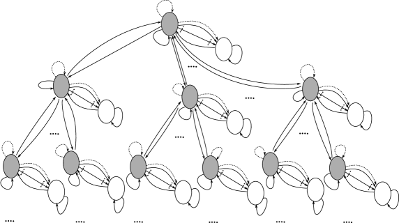
We now build a composite MDP $M$ as considered in (Jaksch etย al., 2010), as a concatenation of $k:=\lfloor\frac{S}{2}\rfloor$ copies of $M^{\prime}$ in the form of an $A^{\prime}$-ary tree, where only one copy contains the good action $a^{\star}$ (see Figure 3). To this end, we first add $A^{\prime}+1$ additional actions so that $M$ has at most $A$ actions per state. For any state s0subscript๐‘ 0s_{0}, one of these new actions connects s0subscript๐‘ 0s_{0} to the root, and the rest connect s0subscript๐‘ 0s_{0} to the leaves. Whereas for any state s1subscript๐‘ 1s_{1}, all new actions make a transition to the same state s1subscript๐‘ 1s_{1}. By construction, the diameter of the composite MDP $M$ does not exceed $2(\frac{D}{4}+\log_{A^{\prime}}k)$, so that MDP $M$ has $2\lfloor\frac{S}{2}\rfloor\leqslant S$ states, $\lfloor\frac{A^{\prime}-1}{2}\rfloor+\lfloor\frac{A^{\prime}-1}{2}\rfloor+1\leqslant A$ actions, and a diameter less than $D$.

Refer to caption
Figure 3: The composite MDP $M$ (Jaksch etย al., 2010)

A.1 Proof of Theorem 9

To derive the claimed result, we derive a lower bound on the regret for the composite MDP presented above. Our analysis is largely built on the techniques used in the proof of (Jaksch etย al., 2010, Theoremย 5). We also closely follow the notations used in (Jaksch etย al., 2010).

Let us assume, as in the proof of (Jaksch etย al., 2010, Theoremย 5), that all states s0subscript๐‘ 0s_{0} are identified so that $M$ is equivalent to an MDP $M^{\prime}$ with $kA^{\prime}$ actions (note that following the same argument as in (Jaksch etย al., 2010), despite the same maximal average reward, learning in $M^{\prime}$ is easier than in $M$, and so any regret lower bound for $M^{\prime}$ implies a lower bound in $M$, too). Note that by construction of $M$, it holds that $\mathbf{V}_{\max}$ in $M$ equals $\mathbf{V}_{\max}$ in $M^{\prime}$. Denote by (s0โ‹†,aโ‹†)subscriptsuperscript๐‘ โ‹†0superscript๐‘Žโ‹†(s^{\star}_{0},a^{\star}) the good copy, i.e., the one containing the good action $a^{\star}$. We assume that $a^{\star}$ is chosen uniformly at random among all actions $\{1,\ldots,k\}\times\{1,\ldots,A^{\prime}\}$. Let $\mathbb{E}_{\star}[\cdot]$ and $\mathbb{E}_{\mathrm{unif}}[\cdot]$ respectively denote the expectation with respect to the random choice of (s0โ‹†,aโ‹†)superscriptsubscript๐‘ 0โ‹†superscript๐‘Žโ‹†(s_{0}^{\star},a^{\star}) and the expectation when there is no good action. Furthermore, let $\mathbb{E}_{a}[\cdot]$ denote the expectation conditioned on $a=a^{\star}$, and introduce $N_{1}$, $N_{0}$, and $N_{0}^{\star}$ as the respective number of visits to s1subscript๐‘ 1s_{1}, s0subscript๐‘ 0s_{0}, and (s0,aโ‹†)subscript๐‘ 0superscript๐‘Žโ‹†(s_{0},a^{\star}).

The proof proceeds in the same steps as in the proof of (Jaksch etย al., 2010, Theoremย 5) up to Equation (36) there, where it is shown that assuming that the initial state is s0subscript๐‘ 0s_{0},

$\displaystyle\mathbb{E}_{a}[N_{1}]$ $\displaystyle\leqslant\mathbb{E}_{a}[N_{0}-N_{0}^{\star}]+(\delta+\varepsilon)D^{\prime}\mathbb{E}_{a}[N_{0}^{\star}]\leqslant T-\mathbb{E}_{\mathrm{unif}}[N_{1}]+\varepsilon D^{\prime}\mathbb{E}_{a}[N_{0}^{\star}]\,,$
$\displaystyle\mathbb{E}_{\mathrm{unif}}[N_{1}]$ $\displaystyle\geqslant\frac{T-D^{\prime}}{2}\,,$

so that the accumulated reward $R_{\mathbb{A},T}$ by the algorithm $\mathbb{A}$ in $M^{\prime}$ up to time step $T$ satisfies

$\displaystyle\mathbb{E}_{a}[R_{\mathbb{A},T}]\leqslant\mathbb{E}_{a}[N_{1}]\leqslant\frac{T+D^{\prime}}{2}+\varepsilon D^{\prime}\mathbb{E}_{a}[N_{0}^{\star}]\,.$

The following lemma, which is a straightforward modification to (Jaksch etย al., 2010, Lemmaย 13), enables us to control $\mathbb{E}_{a}[N_{0}^{\star}]$:

Lemma 18

Let f:{s0,s1}T+1โ†ฆ[0,B]:๐‘“maps-tosuperscriptsubscript๐‘ 0subscript๐‘ 1๐‘‡10๐ตf:\{s_{0},s_{1}\}^{T+1}\mapsto[0,B] be any function defined on any trajectory ๐ฌT+1=(st)1โฉฝtโฉฝT+1subscript๐ฌ๐‘‡1subscriptsubscript๐‘ ๐‘ก1๐‘ก๐‘‡1\boldsymbol{s}_{T+1}=(s_{t})_{1\leqslant t\leqslant T+1} in $M^{\prime}$. Then, for any $\delta\in[0,\tfrac{1}{3}]$, $\varepsilon\in(0,1-2\delta)$, and $a\in\{1,\ldots,kA^{\prime}\}$,

$\displaystyle\mathbb{E}_{a}[f(\boldsymbol{s})]$ $\displaystyle\leqslant\mathbb{E}_{\mathrm{unif}}[f(\boldsymbol{s})]+\varepsilon B\sqrt{\frac{\log(2)\mathbb{E}_{\mathrm{unif}}[N_{0}^{\star}]}{2(\delta+\varepsilon)(1-\delta-\varepsilon)}}\;.$

Noting that $N_{0}^{\star}$ is a function of $\boldsymbol{s}_{T+1}$ satisfying $N_{0}^{\star}\in[0,T]$, by Lemma 18 we deduce

$\displaystyle\mathbb{E}_{a}[N_{0}^{\star}]$ $\displaystyle\leqslant\mathbb{E}_{\mathrm{unif}}[N_{0}^{\star}]+\varepsilon T\sqrt{\frac{\log(2)\mathbb{E}_{\mathrm{unif}}[N_{0}^{\star}]}{2(\delta+\varepsilon)(1-\delta-\varepsilon)}}$
$\displaystyle=\mathbb{E}_{\mathrm{unif}}[N_{0}^{\star}]+\varepsilon\Psi T\sqrt{\frac{\log(2)\mathbb{E}_{\mathrm{unif}}[N_{0}^{\star}]}{2\mathbf{V}_{\max}}}\,,$

where we used $\sqrt{\mathbf{V}_{\max}}=\Psi\sqrt{(\delta+\varepsilon)(1-\varepsilon-\delta)}$. As shown in the proof of (Jaksch etย al., 2010, Theoremย 5), $\sum_{a=1}^{kA^{\prime}}\mathbb{E}_{\mathrm{unif}}[N_{0}^{\star}]\leqslant(T+D^{\prime})/2$ and $\sum_{a=1}^{kA^{\prime}}\sqrt{\mathbb{E}_{\mathrm{unif}}[N_{0}^{\star}]}\leqslant\sqrt{kA^{\prime}(T+D^{\prime})/2}$, so that we finally get, using the relation $\mathbb{E}_{\star}[R_{\mathbb{A},T}]=\frac{1}{kA^{\prime}}\sum_{a=1}^{kA^{\prime}}\mathbb{E}_{a}[R_{\mathbb{A},T}]$,

$\displaystyle\mathbb{E}_{\star}[\mathfrak{R}_{\mathbb{A},T,M^{\prime}}]$ $\displaystyle=\frac{\delta+\varepsilon}{2\delta+\varepsilon}T-\mathbb{E}_{\star}[R_{\mathbb{A},T}]$
$\displaystyle\geqslant\frac{\delta+\varepsilon}{2\delta+\varepsilon}T-\frac{T}{2}-\frac{\varepsilon D^{\prime}T}{2kA^{\prime}}-\frac{\varepsilon D^{\prime 2}}{2kA^{\prime}}$
$\displaystyle-\frac{\varepsilon^{2}\Psi D^{\prime}T}{kA^{\prime}}\sqrt{\frac{\log(2)kA^{\prime}T}{4\mathbf{V}_{\max}}}-\frac{\varepsilon^{2}\Psi D^{\prime}T}{kA^{\prime}}\sqrt{\frac{\log(2)kA^{\prime}D^{\prime}}{4\mathbf{V}_{\max}}}-\frac{D^{\prime}}{2}$
$\displaystyle\geqslant\frac{\varepsilon T}{4\delta+2\varepsilon}-\frac{\varepsilon D^{\prime}}{2kA^{\prime}}(T+D^{\prime})-\frac{0.42\varepsilon^{2}\Psi D^{\prime}T}{\sqrt{kA^{\prime}\mathbf{V}_{\max}}}(\sqrt{T}+\sqrt{D^{\prime}})-\frac{D^{\prime}}{2}\;.$

Noting that the assumption $T\geqslant DSA$ implies $T\geqslant 16D^{\prime}kA^{\prime}$, we deduce that

$\displaystyle\mathbb{E}_{\star}[\mathfrak{R}_{\mathbb{A},T,M^{\prime}}]$ $\displaystyle\geqslant\frac{\varepsilon T}{4\delta+2\varepsilon}-\frac{\varepsilon D^{\prime}T}{2kA^{\prime}}\Bigl{(}1+\frac{1}{16kA^{\prime}}\Big{)}-\frac{0.42\varepsilon^{2}\Psi D^{\prime}T\sqrt{T}}{\sqrt{kA^{\prime}\mathbf{V}_{\max}}}\Bigl{(}1+\frac{1}{4\sqrt{kA^{\prime}}}\Big{)}-\frac{D^{\prime}}{2}\,.$

The first term in the right-hand side of the above satisfies

$\displaystyle\frac{\varepsilon T}{4\delta+2\varepsilon}$ $\displaystyle=\frac{\varepsilon T\Psi}{2}\geqslant\frac{5\varepsilon\mathbf{V}_{\max}T}{6}\,,$

since

$\displaystyle\frac{\Psi}{\mathbf{V}_{\max}}=\frac{2\delta+\varepsilon}{(\delta+\varepsilon)(1-\delta-\varepsilon)}\geqslant 1+\frac{\delta}{\delta+\varepsilon}>\frac{5}{3}\,,$

where we used $\varepsilon\leqslant\frac{\delta}{2}$ in the last step. Hence, we get

$\displaystyle\mathbb{E}_{\star}[\mathfrak{R}_{\mathbb{A},T,M^{\prime}}]\geqslant\frac{5}{6}\varepsilon\mathbf{V}_{\max}T-\frac{\varepsilon D^{\prime}T}{2kA^{\prime}}\Bigl{(}1+\frac{1}{16kA^{\prime}}\Big{)}-\frac{0.42\varepsilon^{2}\Psi D^{\prime}T\sqrt{T}}{\sqrt{kA^{\prime}\mathbf{V}_{\max}}}\Bigl{(}1+\frac{1}{4\sqrt{kA^{\prime}}}\Big{)}-\frac{D^{\prime}}{2}\,.$

In particular, setting $\varepsilon=c\sqrt{\frac{kA^{\prime}}{\mathbf{V}_{\max}T}}$ for some $c$ (which will be determined later) yields

$\displaystyle\mathbb{E}_{\star}[\mathfrak{R}_{\mathbb{A},T,M^{\prime}}]$ $\displaystyle\geqslant\frac{5}{6}c\sqrt{kA^{\prime}\mathbf{V}_{\max}T}-\sqrt{kA^{\prime}\mathbf{V}_{\max}T}\left(\frac{cD^{\prime}}{2kA^{\prime}\mathbf{V}_{\max}}\Bigl{(}1+\frac{1}{16kA^{\prime}}\Big{)}\right)$
$\displaystyle-\sqrt{kA^{\prime}\mathbf{V}_{\max}T}\left(\frac{0.42c^{2}}{kA^{\prime}}\frac{D^{\prime}\Psi}{\mathbf{V}_{\max}^{2}}\Bigl{(}1+\frac{1}{4\sqrt{kA^{\prime}}}\Big{)}\right)-\frac{D^{\prime}}{2}\,.$

To simplify the above bound, note that

$\displaystyle\frac{D^{\prime}}{\mathbf{V}_{\max}}$ $\displaystyle\leqslant\frac{(2\delta+\varepsilon)^{2}}{\delta(\delta+\varepsilon)(1-\delta-\varepsilon)}\leqslant 2\Bigl{(}\frac{2\delta+\varepsilon}{\delta}\Big{)}^{2}\leqslant 12.5\,,$ (7)

where we used $1-\varepsilon-\delta\geqslant\tfrac{1}{2}$ since $\varepsilon\leqslant\frac{\delta}{2}$. Moreover,

$\displaystyle\frac{D^{\prime}\Psi}{\mathbf{V}_{\max}^{2}}$ $\displaystyle=\frac{D^{\prime}\Psi}{\Psi^{4}(\delta+\varepsilon)^{2}(1-\delta-\varepsilon)^{2}}$
$\displaystyle=\frac{(2\delta+\varepsilon)^{3}}{\delta(\delta+\varepsilon)^{2}(1-\delta-\varepsilon)^{2}}\leqslant 4\Bigl{(}\frac{2\delta+\varepsilon}{\delta}\Big{)}^{3}\leqslant 62.5\,.$

Putting these together with the fact that

$\displaystyle\frac{D^{\prime}}{2}\leqslant\frac{\sqrt{D^{\prime}}}{2}\sqrt{\frac{T}{16kA^{\prime}}}\leqslant\frac{\sqrt{12.5/16}}{2}\sqrt{\frac{\mathbf{V}_{\max}T}{kA^{\prime}}}\leqslant 0.45\sqrt{\frac{\mathbf{V}_{\max}T}{kA^{\prime}}}\,,$

which follows from (7), we deduce that

$\displaystyle\mathbb{E}_{\star}[\mathfrak{R}_{\mathbb{A},T,M^{\prime}}]\geqslant\sqrt{kA^{\prime}\mathbf{V}_{\max}T}\Bigl{(}\frac{5c}{6}-\frac{12.5c}{2kA^{\prime}}-\frac{12.5c}{32(kA^{\prime})^{2}}-\frac{26.25c^{2}}{kA^{\prime}}-\frac{6.6c^{2}}{(kA^{\prime})^{3/2}}-\frac{0.45}{kA^{\prime}}\Big{)},$

Taking $c=0.132$ and using the facts $k=\lfloor\tfrac{S}{2}\rfloor\geqslant 5$ and $A^{\prime}=\lfloor\frac{A-1}{2}\rfloor\geqslant 4$ yield the announced result. This completes the proof provided that we show that this choice of $c$ satisfies $\varepsilon\leqslant\frac{\delta}{2}$. To this end, observe that by the assumption $T\geqslant DSA\geqslant\frac{16kA^{\prime}}{\delta}$, it follows that

$\displaystyle\varepsilon=0.132\sqrt{\frac{kA^{\prime}}{\mathbf{V}_{\max}T}}\leqslant\frac{0.132}{4}\sqrt{\frac{\delta}{\mathbf{V}_{\max}}}\leqslant\frac{0.132}{4}\sqrt{\frac{\delta(2\delta+\varepsilon)^{2}}{(\delta+\varepsilon)(1-\delta-\varepsilon)}}\leqslant 0.047(2\delta+\varepsilon)\,,$

so that $\varepsilon\leqslant 0.1\delta$. This concludes the proof. $\Box$

A.2 Proof of Lemma 18

The lemma follows by a slight modification of the proof of (Jaksch etย al., 2010, Lemmaย 13). We recall that according to Equations (49)-(51) in (Jaksch etย al., 2010),

$\displaystyle\mathbb{E}_{a}[f(\boldsymbol{s})]-\mathbb{E}_{\mathrm{unif}}[f(\boldsymbol{s})]$ $\displaystyle\leqslant\frac{B}{2}\sqrt{2\log(2)\texttt{KL}(\mathbb{P}_{\mathrm{unif}},\mathbb{{\mathbb{P}}}_{a})}\,,$ (8)

where

$\displaystyle\texttt{KL}(\mathbb{P}_{\mathrm{unif}},\mathbb{{\mathbb{P}}}_{a})$ =โˆ‘t=1TKLโ€‹(โ„™unifโ€‹(st+1|๐’”t),โ„™aโ€‹(st+1|๐’”t))absentsuperscriptsubscript๐‘ก1๐‘‡KLsubscriptโ„™unifconditionalsubscript๐‘ ๐‘ก1superscript๐’”๐‘กsubscriptโ„™๐‘Žconditionalsubscript๐‘ ๐‘ก1superscript๐’”๐‘ก\displaystyle=\sum_{t=1}^{T}\texttt{KL}(\mathbb{P}_{\mathrm{unif}}(s_{t+1}|\boldsymbol{s}^{t}),{\mathbb{P}}_{a}(s_{t+1}|\boldsymbol{s}^{t}))
=โˆ‘t=1Tโ„™unifโ€‹(st=s0,at=a)โ€‹(ฮดโ€‹logโก(ฮดฮด+ฮต)+(1โˆ’ฮด)โ€‹logโก(1โˆ’ฮด1โˆ’ฮดโˆ’ฮต)).absentsuperscriptsubscript๐‘ก1๐‘‡subscriptโ„™unifformulae-sequencesubscript๐‘ ๐‘กsubscript๐‘ 0subscript๐‘Ž๐‘ก๐‘Ž๐›ฟ๐›ฟ๐›ฟ๐œ€1๐›ฟ1๐›ฟ1๐›ฟ๐œ€\displaystyle=\sum_{t=1}^{T}{\mathbb{P}}_{\mathrm{unif}}(s_{t}=s_{0},a_{t}=a)\left(\delta\log\Bigl{(}\frac{\delta}{\delta+\varepsilon}\Big{)}+(1-\delta)\log\Bigl{(}\frac{1-\delta}{1-\delta-\varepsilon}\Big{)}\right)\,.

Now using the inequality $\texttt{kl}(a,b)\leqslant\frac{(a-b)^{2}}{b(1-b)}$ valid for all $a,b\in(0,1)$ (instead of (Jaksch etย al., 2010, Lemmaย 20)) and noting that ๐”ผunifโ€‹[N0โ‹†]=โˆ‘t=1Tโ„™unifโ€‹(st=s0,at=a)subscript๐”ผunifdelimited-[]superscriptsubscript๐‘0โ‹†superscriptsubscript๐‘ก1๐‘‡subscriptโ„™unifformulae-sequencesubscript๐‘ ๐‘กsubscript๐‘ 0subscript๐‘Ž๐‘ก๐‘Ž\mathbb{E}_{\mathrm{unif}}[N_{0}^{\star}]=\sum_{t=1}^{T}{\mathbb{P}}_{\mathrm{unif}}(s_{t}=s_{0},a_{t}=a), we obtain

$\displaystyle\texttt{KL}(\mathbb{P}_{\mathrm{unif}},\mathbb{{\mathbb{P}}}_{a})=\texttt{kl}(\delta,\delta+\varepsilon)\mathbb{E}_{\mathrm{unif}}[N_{0}^{\star}]\leqslant\frac{\varepsilon^{2}}{(1-\delta)(1-\delta-\varepsilon)}\mathbb{E}_{\mathrm{unif}}[N_{0}^{\star}]\,.$

Plugging this into (8) completes the proof. $\Box$

B Concentration Inequalities

B.1 Proof of Lemmaย 10

Let us recall the fundamental equality

$\displaystyle\forall\lambda\in\mathbb{R},\quad\log\mathbb{E}_{P}[\exp(\lambda(X-\mathbb{E}_{P}[X])]=\sup_{Q\ll P}\bigg{[}\lambda\Big{(}\mathbb{E}_{Q}[X]-\mathbb{E}_{P}[X]\Big{)}-\texttt{KL}(Q,P)\bigg{]}.$

In particular, we obtain on the one hand that (see also (Boucheron etย al., 2013, Lemmaย 2.4))

$\displaystyle\forall Q\ll P,\quad\mathbb{E}_{Q}[f]-\mathbb{E}_{P}[f]$ $\displaystyle\leqslant$ $\displaystyle\min_{\lambda\in\mathbb{R}^{+}}\frac{\varphi_{f}(\lambda)+\texttt{KL}(Q,P)}{\lambda}\,.$

Since $\varphi_{f}(0)=0$, then the right-hand side of the above is non-negative. Let us call it $u$. Now, we note that for any $t$ such that $u\geqslant t\geqslant 0$, by construction of $u$, it holds that $\texttt{KL}(Q,P)\geqslant\varphi_{\star,f}(t)$. Thus, $\{x\geqslant 0:\varphi_{f,\star}(x)>\texttt{KL}(Q,P)\}=(u,\infty)$ and hence, $u=\varphi_{+,f}^{-1}(\texttt{KL}(Q,P))$.

On the other hand, it holds

$\displaystyle\forall Q\ll P,\quad\mathbb{E}_{Q}[f]-\mathbb{E}_{P}[f]$ $\displaystyle\geqslant$ $\displaystyle\max_{\lambda\in\mathbb{R}^{-}}\frac{\varphi_{f}(\lambda)+\texttt{KL}(Q,P)}{\lambda}\,.$

Since $\varphi(0)=0$, then the right-hand side quantity is non-positive. Let us call it $v$. Now, we note that for any $t$ such that $v\leqslant t\leqslant 0$, by construction of $v$, it holds that $\texttt{KL}(Q,P)\geqslant\varphi_{\star,f}(t)$. Thus, $\{x\leqslant 0:\varphi_{\star,f}(x)>\texttt{KL}(Q,P)\}=(-\infty,v)$ and hence, $v=\varphi_{-,f}^{-1}(\texttt{KL}(Q,P))$. $\Box$

B.2 Proof of Corollaryย 11

By a standard Bernstein argument (see for instance (Boucheron etย al., 2013, Sectionย 2.8)), it holds

$\displaystyle\forall\lambda\in[0,3/\mathbb{S}(f)),\quad\varphi_{f}(\lambda)$ $\displaystyle\leqslant$ $\displaystyle\frac{\mathbb{V}_{P}[f]}{2}\frac{\lambda^{2}}{1-\frac{\mathbb{S}(f)\lambda}{3}}\,,$
$\displaystyle\forall x\geqslant 0,\quad\varphi_{\star,f}(x)$ $\displaystyle\geqslant$ $\displaystyle\frac{x^{2}}{2(\mathbb{V}_{P}[f]+\frac{\mathbb{S}(f)}{3}x)}\,.$

Then, a direct computation (solving for $x$ in $\varphi_{\star,f}(x)=t$) shows that

$\displaystyle\varphi_{+,f}^{-1}(t)$ $\displaystyle\leqslant$ $\displaystyle\frac{\mathbb{S}(f)}{3}t+\sqrt{2t\mathbb{V}_{P}[f]+\Big{(}\frac{\mathbb{S}(f)}{3}t\Big{)}^{2}}\leqslant\sqrt{2t\mathbb{V}_{P}[f]}+\frac{2}{3}t\mathbb{S}(f)\,,$
$\displaystyle\varphi_{-,f}^{-1}(t)$ $\displaystyle\geqslant$ $\displaystyle\frac{\mathbb{S}(f)}{3}t-\sqrt{2t\mathbb{V}_{P}[f]+\Big{(}\frac{\mathbb{S}(f)}{3}t\Big{)}^{2}}\geqslant-\sqrt{2t\mathbb{V}_{P}[f]}\,,$

where we used that $\sqrt{a+b}\leqslant\sqrt{a}+\sqrt{b}$ for $a,b\geqslant 0$. Combining these bounds, we get

$\displaystyle\mathbb{E}_{Q}[f]-\mathbb{E}_{P}[f]$ $\displaystyle\leqslant$ $\displaystyle\sqrt{2\mathbb{V}_{P}[f]\texttt{KL}(Q,P)}+\frac{2}{3}\mathbb{S}(f)\texttt{KL}(Q,P)\,,$
$\displaystyle\mathbb{E}_{P}[f]-\mathbb{E}_{Q}[f]$ $\displaystyle\leqslant$ $\displaystyle\sqrt{2\mathbb{V}_{P}[f]\texttt{KL}(Q,P)}\,.$

$\Box$

B.3 Proof of Lemma 12

If $\mathbb{E}_{Q}[f]\leqslant\mathbb{E}_{P}[f]$, then the result holds trivially. We thus assume that $\mathbb{E}_{Q}[f]>\mathbb{E}_{P}[f]$. It is straightforward to verify that

$\displaystyle\mathbb{E}_{Q}[f]-\mathbb{E}_{P}[f]$ $\displaystyle=\sum_{x:Q(x)\geqslant P(x)}(f(x)-\mathbb{E}_{Q}[f])(Q(x)-P(x))+\sum_{x:Q(x)<P(x)}(f(x)-\mathbb{E}_{P}[f])(Q(x)-P(x))$
$\displaystyle+\sum_{x:P(x)>Q(x)}(\mathbb{E}_{P}[f]-\mathbb{E}_{Q}[f])(Q(x)-P(x))\;.$ (9)

The first term in the right-hand side of (9) is upper bounded as

$\displaystyle\sum_{x:Q(x)\geqslant P(x)}(f(x)-\mathbb{E}_{Q}[f])$ $\displaystyle(Q(x)-P(x))=\sum_{x:Q(x)\geqslant P(x)}\sqrt{Q(x)}(f(x)-\mathbb{E}_{Q}[f])\frac{Q(x)-P(x)}{\sqrt{Q(x)}}$
$\displaystyle\stackrel{{\scriptstyle(a)}}{{\leqslant}}\sqrt{\sum_{x:Q(x)\geqslant P(x)}Q(x)(f(x)-\mathbb{E}_{Q}[f])^{2}}\sqrt{\sum_{x:Q(x)\geqslant P(x)}\frac{(Q(x)-P(x))^{2}}{Q(x)}}$
$\displaystyle\stackrel{{\scriptstyle(b)}}{{\leqslant}}\sqrt{{\mathcal{V}}_{Q,P}(f)}\sqrt{2\texttt{KL}(P,Q)}\;,$ (10)

where (a) follows from Cauchy-Schwarz inequality and (b) follows from Lemma 22.

Similarly, the second term in (9) satisfies

$\displaystyle\sum_{x:Q(x)<P(x)}(f(x)-\mathbb{E}_{P}[f])(Q(x)-P(x))$ $\displaystyle=\sum_{x:Q(x)<P(x)}\sqrt{P(x)}(f(x)-\mathbb{E}_{P}[f])\frac{Q(x)-P(x)}{\sqrt{P(x)}}$
$\displaystyle\leqslant\sqrt{{\mathcal{V}}_{P,Q}(f)}\sqrt{2\texttt{KL}(P,Q)}\;.$ (11)

Finally, we bound the last term in (9):

$\displaystyle(\mathbb{E}_{P}[f]-\mathbb{E}_{Q}[f])\sum_{x:P(x)>Q(x)}(Q(x)-P(x))$ $\displaystyle\stackrel{{\scriptstyle(a)}}{{=}}\frac{1}{2}(\mathbb{E}_{Q}[f]-\mathbb{E}_{P}[f])\|P-Q\|_{1}$
$\displaystyle\leqslant\frac{1}{2}\mathbb{S}(f)\|P-Q\|_{1}^{2}\stackrel{{\scriptstyle(b)}}{{\leqslant}}\mathbb{S}(f)\texttt{KL}(P,Q)\;,$ (12)

where (a) follows from the fact that for any pair of distributions $U,V\in{\mathcal{P}}(\mathcal{X})$, it holds that $\sum_{x\in{\mathcal{X}}}|U(x)-V(x)|=2\sum_{x:U(x)\geqslant V(x)}(U(x)-V(x))$, and where (b) follows from Pinskerโ€™s inequality. The proof is concluded by combining (10), (11), and (12). $\Box$

B.4 Proof of Lemma 13

Statement (i) is a direct consequence of the definition of ${\mathcal{V}}_{P,Q}$. We next prove statement (ii). Observe that Lemma 22 implies that for all $x\in{\mathcal{X}}$

$\displaystyle|P(x)-Q(x)|\leqslant\sqrt{2\max(P(x),Q(x))\texttt{KL}(Q,P)}\;.$

Hence,

$\displaystyle{\mathcal{V}}_{P,Q}(f)$ $\displaystyle=\sum_{x:P(x)\geqslant Q(x)}P(x)(f(x)-\mathbb{E}_{P}[f])^{2}$
$\displaystyle\leqslant\sum_{x:P(x)\geqslant Q(x)}Q(x)(f(x)-\mathbb{E}_{P}[f])^{2}+\sqrt{2\texttt{KL}(Q,P)}\sum_{x:P(x)\geqslant Q(x)}\sqrt{P(x)}(f(x)-\mathbb{E}_{P}[f])^{2}\;.$ (13)

The first term in the right-hand side of (13) is bounded as follows:

$\displaystyle\sum_{x:P(x)\geqslant Q(x)}Q(x)(f(x)-\mathbb{E}_{P}[f])^{2}$ $\displaystyle\leqslant 2\sum_{x:P(x)\geqslant Q(x)}Q(x)(f(x)-\mathbb{E}_{Q}[f])^{2}+2(\mathbb{E}_{Q}[f]-\mathbb{E}_{P}[f])^{2}$
$\displaystyle\leqslant 2\mathbb{V}_{Q}(f)+2(\mathbb{E}_{Q}[f]-\mathbb{E}_{P}[f])^{2}\;.$

Note that

$$(\mathbb{E}_{Q}[f]-\mathbb{E}_{P}[f])^{2}\leqslant\mathbb{S}(f)^{2}\|P-Q\|_{1}^{2}\leqslant 2\mathbb{S}(f)^{2}\texttt{KL}(Q,P)\;,$$

which further gives

$\displaystyle\sum_{x:P(x)\geqslant Q(x)}Q(x)(f(x)-\mathbb{E}_{P}[f])^{2}$ $\displaystyle\leqslant 2\mathbb{V}_{Q}(f)+4\mathbb{S}(f)^{2}\texttt{KL}(Q,P)\;.$

Now we consider the second term in (13). First observe that

$\displaystyle\sum_{x:P(x)\geqslant Q(x)}\sqrt{P(x)}(f(x)-\mathbb{E}_{P}[f])^{2}$ $\displaystyle\leqslant\sqrt{\sum_{x:P(x)\geqslant Q(x)}P(x)(f(x)-\mathbb{E}_{P}[f])^{2}}\sqrt{\sum_{x}(f(x)-\mathbb{E}_{P}[f])^{2}}$
$\displaystyle\leqslant\sqrt{{\mathcal{V}}_{P,Q}(f)}\mathbb{S}(f)\sqrt{|{\mathcal{X}}|}\;,$

thanks to Cauchy-Schwarz inequality. Hence, the second term in (13) is upper bounded by

$$\mathbb{S}(f)\sqrt{2|{\mathcal{X}}|{\mathcal{V}}_{P,Q}(f)\texttt{KL}(Q,P)}\;.$$

Combining the previous bounds together, we get

$\displaystyle{\mathcal{V}}_{P,Q}(f)\leqslant 2\mathbb{V}_{Q}(f)+4\mathbb{S}(f)^{2}\texttt{KL}(Q,P)+\mathbb{S}(f)\sqrt{2|{\mathcal{X}}|{\mathcal{V}}_{P,Q}(f)\texttt{KL}(Q,P)}\;,$

which leads to

$\displaystyle\Bigl{(}\sqrt{{\mathcal{V}}_{P,Q}(f)}-\mathbb{S}(f)\sqrt{|{\mathcal{X}}|\texttt{KL}(Q,P)/2}\Big{)}^{2}\leqslant 2\mathbb{V}_{Q}(f)+\mathbb{S}(f)^{2}(|{\mathcal{X}}|/2+4)\texttt{KL}(Q,P)\;,$

so that using the inequality $\sqrt{a+b}\leqslant\sqrt{a}+\sqrt{b}$, we finally obtain

$\displaystyle\sqrt{{\mathcal{V}}_{Q,P}(f)}$ $\displaystyle\leqslant\sqrt{2\mathbb{V}_{Q}(f)+\mathbb{S}(f)^{2}(|{\mathcal{X}}|/2+4)\texttt{KL}(Q,P)}+\mathbb{S}(f)\sqrt{|{\mathcal{X}}|\texttt{KL}(Q,P)/2}$
$\displaystyle\leqslant\sqrt{2\mathbb{V}_{Q}(f)}+\mathbb{S}(f)(\sqrt{2|{\mathcal{X}}|}+2)\sqrt{\texttt{KL}(Q,P)}\;.$

The proof is completed by observing that $\sqrt{2|{\mathcal{X}}|}+2\leqslant 3\sqrt{|{\mathcal{X}}|}$ for $|{\mathcal{X}}|\geqslant 2$. $\Box$

B.5 Proof of Lemma 16

Let $\delta\in(0,1)$ and (s,a)โˆˆ๐’ฎร—๐’œ๐‘ ๐‘Ž๐’ฎ๐’œ(s,a)\in{\mathcal{S}}\times{\mathcal{A}}. Consider an episode $k\geqslant 1$ such that $M\in{\mathcal{M}}_{k}$, and define $\hat{p}_{k}=\hat{p}_{k}(\cdot|s,a)$, $p=p(\cdot|s,a)$, and Nk=Nkโ€‹(s,a)subscript๐‘๐‘˜subscript๐‘๐‘˜๐‘ ๐‘ŽN_{k}=N_{k}(s,a). Observe that by a Bernstein-like inequality (Dann etย al., 2017, Lemmaย F.2), we have: for all sโ€ฒโˆˆ๐’ฎsuperscript๐‘ โ€ฒ๐’ฎs^{\prime}\in{\mathcal{S}}, with probability at least $1-\delta$,

p^kโ€‹(sโ€ฒ)โˆ’pโ€‹(sโ€ฒ)โฉฝ2โ€‹pโ€‹(sโ€ฒ)โ€‹CbNk+2โ€‹CbNk,subscript^๐‘๐‘˜superscript๐‘ โ€ฒ๐‘superscript๐‘ โ€ฒ2๐‘superscript๐‘ โ€ฒsubscript๐ถ๐‘subscript๐‘๐‘˜2subscript๐ถ๐‘subscript๐‘๐‘˜\displaystyle\hat{p}_{k}(s^{\prime})-p(s^{\prime})\leqslant\sqrt{\frac{2p(s^{\prime})C_{b}}{N_{k}}}+\frac{2C_{b}}{N_{k}}\;,

with $C_{b}=C_{b}(t,\delta):=\log(3\log(\max(e,t))/\delta)$. It then follows that with probability at least $1-\delta$,

$\displaystyle\mathbb{V}_{\hat{p}_{k}}$ (f)=โˆ‘sโ€ฒp^kโ€‹(sโ€ฒ)โ€‹(fโ€‹(sโ€ฒ)โˆ’๐”ผp^kโ€‹[f])2๐‘“subscriptsuperscript๐‘ โ€ฒsubscript^๐‘๐‘˜superscript๐‘ โ€ฒsuperscript๐‘“superscript๐‘ โ€ฒsubscript๐”ผsubscript^๐‘๐‘˜delimited-[]๐‘“2\displaystyle(f)=\sum_{s^{\prime}}\hat{p}_{k}(s^{\prime})(f(s^{\prime})-\mathbb{E}_{\hat{p}_{k}}[f])^{2}
โฉฝโˆ‘sโ€ฒpโ€‹(sโ€ฒ)โ€‹(fโ€‹(sโ€ฒ)โˆ’๐”ผp^kโ€‹[f])2+2โ€‹CbNkโ€‹โˆ‘sโ€ฒpโ€‹(sโ€ฒ)โ€‹(fโ€‹(sโ€ฒ)โˆ’๐”ผp^kโ€‹[f])2+2โ€‹CbNkโ€‹โˆ‘sโ€ฒ(fโ€‹(sโ€ฒ)โˆ’๐”ผp^kโ€‹[f])2absentsubscriptsuperscript๐‘ โ€ฒ๐‘superscript๐‘ โ€ฒsuperscript๐‘“superscript๐‘ โ€ฒsubscript๐”ผsubscript^๐‘๐‘˜delimited-[]๐‘“22subscript๐ถ๐‘subscript๐‘๐‘˜subscriptsuperscript๐‘ โ€ฒ๐‘superscript๐‘ โ€ฒsuperscript๐‘“superscript๐‘ โ€ฒsubscript๐”ผsubscript^๐‘๐‘˜delimited-[]๐‘“22subscript๐ถ๐‘subscript๐‘๐‘˜subscriptsuperscript๐‘ โ€ฒsuperscript๐‘“superscript๐‘ โ€ฒsubscript๐”ผsubscript^๐‘๐‘˜delimited-[]๐‘“2\displaystyle\leqslant\sum_{s^{\prime}}p(s^{\prime})(f(s^{\prime})-\mathbb{E}_{\hat{p}_{k}}[f])^{2}+\sqrt{\frac{2C_{b}}{N_{k}}}\sum_{s^{\prime}}\sqrt{p(s^{\prime})}(f(s^{\prime})-\mathbb{E}_{\hat{p}_{k}}[f])^{2}+\frac{2C_{b}}{N_{k}}\sum_{s^{\prime}}(f(s^{\prime})-\mathbb{E}_{\hat{p}_{k}}[f])^{2}
โฉฝโˆ‘sโ€ฒpโ€‹(sโ€ฒ)โ€‹(fโ€‹(sโ€ฒ)โˆ’๐”ผp^kโ€‹[f])2โŸZ1+2โ€‹CbNkโ€‹โˆ‘sโ€ฒpโ€‹(sโ€ฒ)โ€‹(fโ€‹(sโ€ฒ)โˆ’๐”ผp^kโ€‹[f])2โŸZ2+2โ€‹Cbโ€‹Sโ€‹๐•Šโ€‹(f)2Nk.absentsubscriptโŸsubscriptsuperscript๐‘ โ€ฒ๐‘superscript๐‘ โ€ฒsuperscript๐‘“superscript๐‘ โ€ฒsubscript๐”ผsubscript^๐‘๐‘˜delimited-[]๐‘“2subscript๐‘12subscript๐ถ๐‘subscript๐‘๐‘˜subscriptโŸsubscriptsuperscript๐‘ โ€ฒ๐‘superscript๐‘ โ€ฒsuperscript๐‘“superscript๐‘ โ€ฒsubscript๐”ผsubscript^๐‘๐‘˜delimited-[]๐‘“2subscript๐‘22subscript๐ถ๐‘๐‘†๐•Šsuperscript๐‘“2subscript๐‘๐‘˜\displaystyle\leqslant\underbrace{\sum_{s^{\prime}}p(s^{\prime})(f(s^{\prime})-\mathbb{E}_{\hat{p}_{k}}[f])^{2}}_{Z_{1}}+\sqrt{\frac{2C_{b}}{N_{k}}}\underbrace{\sum_{s^{\prime}}\sqrt{p(s^{\prime})}(f(s^{\prime})-\mathbb{E}_{\hat{p}_{k}}[f])^{2}}_{Z_{2}}+\frac{2C_{b}S\mathbb{S}(f)^{2}}{N_{k}}\;. (14)

Next we bound $Z_{1}$ and $Z_{2}$. Observe that

$\displaystyle Z_{1}$ โฉฝ2โ€‹โˆ‘sโ€ฒpโ€‹(sโ€ฒ)โ€‹(fโ€‹(sโ€ฒ)โˆ’๐”ผpโ€‹[f])2+2โ€‹(๐”ผpโ€‹[f]โˆ’๐”ผp^kโ€‹[f])2absent2subscriptsuperscript๐‘ โ€ฒ๐‘superscript๐‘ โ€ฒsuperscript๐‘“superscript๐‘ โ€ฒsubscript๐”ผ๐‘delimited-[]๐‘“22superscriptsubscript๐”ผ๐‘delimited-[]๐‘“subscript๐”ผsubscript^๐‘๐‘˜delimited-[]๐‘“2\displaystyle\leqslant 2\sum_{s^{\prime}}p(s^{\prime})(f(s^{\prime})-\mathbb{E}_{p}[f])^{2}+2(\mathbb{E}_{p}[f]-\mathbb{E}_{\hat{p}_{k}}[f])^{2}
$\displaystyle\leqslant 2\mathbb{V}_{p}(f)+4\mathbb{S}(f)^{2}\texttt{KL}(\hat{p}_{k},p)\;,$

where the last inequality follows from

$\displaystyle(\mathbb{E}_{p}[f]-\mathbb{E}_{\hat{p}_{k}}[f])^{2}\leqslant\mathbb{S}(f)^{2}\|p-\hat{p}_{k}\|_{1}^{2}\leqslant 2\mathbb{S}(f)^{2}\texttt{KL}(\hat{p}_{k},p)\;.$ (15)

For $Z_{2}$ we have

Z2โฉฝ2โ€‹โˆ‘sโ€ฒpโ€‹(sโ€ฒ)โ€‹(fโ€‹(sโ€ฒ)โˆ’๐”ผpโ€‹[f])2+2โ€‹(๐”ผpโ€‹[f]โˆ’๐”ผp^kโ€‹[f])2โ€‹โˆ‘sโ€ฒpโ€‹(sโ€ฒ).subscript๐‘22subscriptsuperscript๐‘ โ€ฒ๐‘superscript๐‘ โ€ฒsuperscript๐‘“superscript๐‘ โ€ฒsubscript๐”ผ๐‘delimited-[]๐‘“22superscriptsubscript๐”ผ๐‘delimited-[]๐‘“subscript๐”ผsubscript^๐‘๐‘˜delimited-[]๐‘“2subscriptsuperscript๐‘ โ€ฒ๐‘superscript๐‘ โ€ฒ\displaystyle Z_{2}\leqslant 2\sum_{s^{\prime}}\sqrt{p(s^{\prime})}(f(s^{\prime})-\mathbb{E}_{p}[f])^{2}+2(\mathbb{E}_{p}[f]-\mathbb{E}_{\hat{p}_{k}}[f])^{2}\sum_{s^{\prime}}\sqrt{p(s^{\prime})}\;.

Now, using Cauchy-Schwarz inequality

โˆ‘sโ€ฒpโ€‹(sโ€ฒ)โ€‹(fโ€‹(sโ€ฒ)โˆ’๐”ผpโ€‹[f])2subscriptsuperscript๐‘ โ€ฒ๐‘superscript๐‘ โ€ฒsuperscript๐‘“superscript๐‘ โ€ฒsubscript๐”ผ๐‘delimited-[]๐‘“2\displaystyle\sum_{s^{\prime}}\sqrt{p(s^{\prime})}(f(s^{\prime})-\mathbb{E}_{p}[f])^{2} โฉฝโˆ‘sโ€ฒpโ€‹(sโ€ฒ)โ€‹(fโ€‹(sโ€ฒ)โˆ’๐”ผpโ€‹[f])2โ€‹โˆ‘sโ€ฒ(fโ€‹(sโ€ฒ)โˆ’๐”ผpโ€‹[f])2absentsubscriptsuperscript๐‘ โ€ฒ๐‘superscript๐‘ โ€ฒsuperscript๐‘“superscript๐‘ โ€ฒsubscript๐”ผ๐‘delimited-[]๐‘“2subscriptsuperscript๐‘ โ€ฒsuperscript๐‘“superscript๐‘ โ€ฒsubscript๐”ผ๐‘delimited-[]๐‘“2\displaystyle\leqslant\sqrt{\sum_{s^{\prime}}p(s^{\prime})(f(s^{\prime})-\mathbb{E}_{p}[f])^{2}\sum_{s^{\prime}}(f(s^{\prime})-\mathbb{E}_{p}[f])^{2}}
$\displaystyle\leqslant\sqrt{S\mathbb{V}_{p}(f)}\mathbb{S}(f)\;,$

so that using (15), we deduce that

$\displaystyle Z_{2}$ โฉฝ2โ€‹๐•Šโ€‹(f)โ€‹Sโ€‹๐•pโ€‹(f)+4โ€‹๐•Šโ€‹(f)2โ€‹KLโ€‹(p^k,p)โ€‹โˆ‘sโ€ฒpโ€‹(sโ€ฒ)absent2๐•Š๐‘“๐‘†subscript๐•๐‘๐‘“4๐•Šsuperscript๐‘“2KLsubscript^๐‘๐‘˜๐‘subscriptsuperscript๐‘ โ€ฒ๐‘superscript๐‘ โ€ฒ\displaystyle\leqslant 2\mathbb{S}(f)\sqrt{S\mathbb{V}_{p}(f)}+4\mathbb{S}(f)^{2}\texttt{KL}(\hat{p}_{k},p)\sum_{s^{\prime}}\sqrt{p(s^{\prime})}
$\displaystyle\leqslant 2\mathbb{S}(f)\sqrt{S\mathbb{V}_{p}(f)}+4\mathbb{S}(f)^{2}\texttt{KL}(\hat{p}_{k},p)\sqrt{S}\;,$

where the last inequality follows from Jensenโ€™s inequality:

โˆ‘sโ€ฒpโ€‹(sโ€ฒ)=โˆ‘sโ€ฒpโ€‹(sโ€ฒ)โ€‹1pโ€‹(sโ€ฒ)โฉฝโˆ‘sโ€ฒpโ€‹(sโ€ฒ)pโ€‹(sโ€ฒ)=S.subscriptsuperscript๐‘ โ€ฒ๐‘superscript๐‘ โ€ฒsubscriptsuperscript๐‘ โ€ฒ๐‘superscript๐‘ โ€ฒ1๐‘superscript๐‘ โ€ฒsubscriptsuperscript๐‘ โ€ฒ๐‘superscript๐‘ โ€ฒ๐‘superscript๐‘ โ€ฒ๐‘†\sum_{s^{\prime}}\sqrt{p(s^{\prime})}=\sum_{s^{\prime}}p(s^{\prime})\sqrt{\frac{1}{p(s^{\prime})}}\leqslant\sum_{s^{\prime}}\sqrt{\frac{p(s^{\prime})}{p(s^{\prime})}}=\sqrt{S}\;.

Putting together, we deduce that with probability at least $1-\delta$,

$\displaystyle\mathbb{V}_{\hat{p}_{k}}(f)$ $\displaystyle\leqslant 2\mathbb{V}_{p}(f)+2\mathbb{S}(f)\sqrt{\frac{2SC_{b}}{N_{k}}}\Bigl{(}\sqrt{\mathbb{V}_{p}(f)}+2\mathbb{S}(f)\texttt{KL}(\hat{p}_{k},p)\Big{)}+\mathbb{S}(f)^{2}\Bigl{(}4\texttt{KL}(\hat{p}_{k},p)+\frac{2SC_{b}}{N_{k}}\Big{)}\;.$

Noting that $M\in{\mathcal{M}}_{k}$, we obtain

$\displaystyle\mathbb{V}_{\hat{p}_{k}}(f)$ $\displaystyle\leqslant 2\mathbb{V}_{p}(f)+\mathbb{S}(f)\sqrt{\frac{8S\mathbb{V}_{p}(f)C_{b}}{N_{k}}}+4\mathbb{S}(f)^{2}\frac{\sqrt{2SC_{b}}C_{p}}{N_{k}^{3/2}}+\frac{(4C_{p}+2SC_{b})\mathbb{S}(f)^{2}}{N_{k}}$
$\displaystyle\leqslant 2\mathbb{V}_{p}(f)+\mathbb{S}(f)\sqrt{\frac{8S\mathbb{V}_{p}(f)C_{b}}{N_{k}}}+\frac{S\mathbb{S}(f)^{2}}{N_{k}}(16B\sqrt{2SC_{b}}+16B+2C_{b})$
$\displaystyle\leqslant 2\mathbb{V}_{p}(f)+\mathbb{S}(f)\sqrt{\frac{8S\mathbb{V}_{p}(f)B}{N_{k}}}+\frac{36S^{3/2}B^{3/2}\mathbb{S}(f)^{2}}{N_{k}}\;,$

with probability at least $1-\delta$, where we used $C_{p}=4SB$, $C_{b}\leqslant B$, and $S\geqslant 2$. The proof is concluded by observing that

$\displaystyle\sqrt{\mathbb{V}_{\hat{p}_{k}}(f)}$ $\displaystyle\leqslant\sqrt{2\mathbb{V}_{p}(f)}+\mathbb{S}(f)\sqrt{\frac{SB}{N_{k}}}+6\mathbb{S}(f)B\sqrt{\frac{S^{3/2}}{N_{k}}}$
$\displaystyle\leqslant\sqrt{2\mathbb{V}_{p}(f)}+\frac{6S\mathbb{S}(f)B}{\sqrt{N_{k}}}\;,$

with probability at least $1-\delta$. $\Box$

C Regret Upper Bound for KL-Ucrl

In this section, we provide the proof of the main result (Theorem 14). We will try to closely follow the notations used in the proof of (Jaksch etย al., 2010, Theoremย 2).

We first recall the following result indicating that the true model belongs to the set of plausible MDPs with high probability. Recall that for $\delta\in(0,1]$ and $t\in{\mathbb{N}}$,

$\displaystyle C_{\mu}:=C_{\mu}(T,\delta)$ $\displaystyle=\log(4SA\log(T)/\delta)/1.99\,,$
$\displaystyle C_{p}:=C_{p}(T,\delta)$ $\displaystyle=S\left(B+\log(G)(1+1/G)\right)\,,$

where

$\displaystyle B:$ $\displaystyle=B(T,\delta)=\log(2eS^{2}A\log(T)/\delta)\,,$ (16)
$\displaystyle G:$ $\displaystyle=G(T,\delta)=B+1/\log(T)\,.$

Moreover, observe that $C_{p}\leqslant 4SB$.

Lemma 19 ((Filippi etย al., 2010, Propositionย 1))

For all $T\geqslant 1$ and $\delta>0$, and for any pair (s,a)๐‘ ๐‘Ž(s,a), it holds that

โ„™โ€‹(โˆ€tโฉฝT,|ฮผ^tโ€‹(s,a)โˆ’ฮผโ€‹(s,a)|โฉฝCฮผ/Ntโ€‹(s,a))โ„™formulae-sequencefor-all๐‘ก๐‘‡subscript^๐œ‡๐‘ก๐‘ ๐‘Ž๐œ‡๐‘ ๐‘Žsubscript๐ถ๐œ‡subscript๐‘๐‘ก๐‘ ๐‘Ž\displaystyle{\mathbb{P}}\Bigl{(}\forall t\leqslant T,\;|\hat{\mu}_{t}(s,a)-\mu(s,a)|\leqslant\sqrt{C_{\mu}/N_{t}(s,a)}\Big{)} $\displaystyle\geqslant 1-\frac{\delta}{SA}\,,$
$\displaystyle{\mathbb{P}}\Bigl{(}\forall t\leqslant T,\;N_{t}(s,a)\emph{{KL}}(\hat{p}_{t}(s,a),p(\cdot|s,a))\leqslant C_{p}\Big{)}$ $\displaystyle\geqslant 1-\frac{\delta}{SA}\,.$

In particular, ${\mathbb{P}}(\forall t\leqslant T,\;M\in{\mathcal{M}}_{t})\geqslant 1-2\delta$.

Next we prove the theorem.

Proof (of Theorem 14). Let $T\geqslant 1$ and $\delta\in(0,1)$. Fix algorithm $\mathbb{A}=\textsc{{KL-Ucrl}}$. Denote by $m(T)$ the number of episodes started by KL-Ucrlย up to time step $T$ (hence, $1\leqslant k\leqslant m(T)$).

By applying Azuma-Hoeffding inequality, as in the proof of (Jaksch etย al., 2010, Theoremย 2), we deduce that

$\displaystyle\mathfrak{R}_{\mathbb{A},T}$ =Tโ€‹gโ‹†โˆ’โˆ‘t=1Trโ€‹(st,at)โฉฝโˆ‘s,aNTโ€‹(s,a)โ€‹(gโ‹†โˆ’ฮผโ€‹(s,a))+12โ€‹Tโ€‹logโก(1/ฮด),absent๐‘‡superscript๐‘”โ‹†superscriptsubscript๐‘ก1๐‘‡๐‘Ÿsubscript๐‘ ๐‘กsubscript๐‘Ž๐‘กsubscript๐‘ ๐‘Žsubscript๐‘๐‘‡๐‘ ๐‘Žsuperscript๐‘”โ‹†๐œ‡๐‘ ๐‘Ž12๐‘‡1๐›ฟ\displaystyle=Tg^{\star}-\sum_{t=1}^{T}r(s_{t},a_{t})\leqslant\sum_{s,a}N_{T}(s,a)(g^{\star}-\mu(s,a))+\sqrt{\tfrac{1}{2}T\log(1/\delta)}\;,

with probability at least $1-\delta$. The regret up to time $T$ can be decomposed as the sum of the regret incurred in various episodes. Let $\Delta_{k}$ denote the regret in episode $k$:

ฮ”k:=โˆ‘s,avkโ€‹(s,a)โ€‹(gโ‹†โˆ’ฮผโ€‹(s,a)).assignsubscriptฮ”๐‘˜subscript๐‘ ๐‘Žsubscript๐‘ฃ๐‘˜๐‘ ๐‘Žsuperscript๐‘”โ‹†๐œ‡๐‘ ๐‘Ž\displaystyle\Delta_{k}:=\sum_{s,a}v_{k}(s,a)(g^{\star}-\mu(s,a))\;.

Therefore, Lemma 19 implies that with probability at least $1-3\delta$,

$\displaystyle\mathfrak{R}_{\mathbb{A},T}$ $\displaystyle\leqslant\sum_{k=1}^{m(T)}\Delta_{k}\mathbb{I}\{M\in{\mathcal{M}}_{k}\}+\sqrt{\tfrac{1}{2}T\log(1/\delta)}\;.$

Next we derive an upper bound on the first term in the right-hand side of the above inequality. Consider an episode $k\geqslant 1$ such that $M\in{\mathcal{M}}_{k}$. The state-action pair (s,a)๐‘ ๐‘Ž(s,a) is considered as sufficiently sampled in episode $k$ if its number of observations satisfies Nkโ€‹(s,a)โฉพโ„“s,asubscript๐‘๐‘˜๐‘ ๐‘Žsubscriptโ„“๐‘ ๐‘ŽN_{k}(s,a)\geqslant\ell_{s,a}, with

โ„“s,a=โ„“s,aโ€‹(T,ฮด):=maxโก{128โ€‹Sโ€‹Bโ€‹maxโก(ฮจ2,1)ฯ†โ€‹(s,a)2,โ€‰32โ€‹Sโ€‹Bโ€‹(logโก(D)logโก(1/ฮณ))2},โˆ€s,a,formulae-sequencesubscriptโ„“๐‘ ๐‘Žsubscriptโ„“๐‘ ๐‘Ž๐‘‡๐›ฟassign128๐‘†๐ตsuperscriptฮจ21๐œ‘superscript๐‘ ๐‘Ž232๐‘†๐ตsuperscript๐ท1๐›พ2for-all๐‘ ๐‘Ž\ell_{s,a}=\ell_{s,a}(T,\delta):=\max\Bigl{\{}\frac{128SB\max(\Psi^{2},1)}{\varphi(s,a)^{2}},\,32SB\Big{(}\frac{\log(D)}{\log(1/\gamma)}\Big{)}^{2}\Big{\}},\quad\forall s,a\,,

where $B$ is given in (16), and where $\gamma$ denotes the contraction factor of the mapping induced by the transition probability matrix $P_{\star}$ of the optimal policy ($\gamma$ can be determined as a function of elements of $P_{\star}$).

Now consider the case where all state-action pairs are sufficiently sampled in episode $k$ (we analyse the case where some pairs are under-sampled (i.e., not sufficiently sampled) at the end of the proof). We have

|ฮผ~kโ€‹(s,a)โˆ’ฮผโ€‹(s,a)|subscript~๐œ‡๐‘˜๐‘ ๐‘Ž๐œ‡๐‘ ๐‘Ž\displaystyle|\tilde{\mu}_{k}(s,a)-\mu(s,a)| โฉฝ|ฮผ~kโ€‹(s,a)โˆ’ฮผ^kโ€‹(s,a)|+|ฮผ^kโ€‹(s,a)โˆ’ฮผโ€‹(s,a)|โฉฝ2โ€‹CฮผNkโ€‹(s,a)+.absentsubscript~๐œ‡๐‘˜๐‘ ๐‘Žsubscript^๐œ‡๐‘˜๐‘ ๐‘Žsubscript^๐œ‡๐‘˜๐‘ ๐‘Ž๐œ‡๐‘ ๐‘Ž2subscript๐ถ๐œ‡subscript๐‘๐‘˜superscript๐‘ ๐‘Ž\displaystyle\leqslant|\tilde{\mu}_{k}(s,a)-\hat{\mu}_{k}(s,a)|+|\hat{\mu}_{k}(s,a)-\mu(s,a)|\leqslant 2\sqrt{\frac{C_{\mu}}{N_{k}(s,a)^{+}}}\;.

Hence,

$\displaystyle\Delta_{k}$ =โˆ‘s,avkโ€‹(s,a)โ€‹(gโ‹†โˆ’ฮผ~kโ€‹(s,a))+โˆ‘s,avkโ€‹(s,a)โ€‹(ฮผ~kโ€‹(s,a)โˆ’ฮผโ€‹(s,a))absentsubscript๐‘ ๐‘Žsubscript๐‘ฃ๐‘˜๐‘ ๐‘Žsuperscript๐‘”โ‹†subscript~๐œ‡๐‘˜๐‘ ๐‘Žsubscript๐‘ ๐‘Žsubscript๐‘ฃ๐‘˜๐‘ ๐‘Žsubscript~๐œ‡๐‘˜๐‘ ๐‘Ž๐œ‡๐‘ ๐‘Ž\displaystyle=\sum_{s,a}v_{k}(s,a)(g^{\star}-\tilde{\mu}_{k}(s,a))+\sum_{s,a}v_{k}(s,a)(\tilde{\mu}_{k}(s,a)-\mu(s,a))
โฉฝโˆ‘s,avkโ€‹(s,a)โ€‹(gโ‹†โˆ’ฮผ~kโ€‹(s,a))+2โ€‹Cฮผโ€‹โˆ‘s,avkโ€‹(s,a)Nkโ€‹(s,a)+.absentsubscript๐‘ ๐‘Žsubscript๐‘ฃ๐‘˜๐‘ ๐‘Žsuperscript๐‘”โ‹†subscript~๐œ‡๐‘˜๐‘ ๐‘Ž2subscript๐ถ๐œ‡subscript๐‘ ๐‘Žsubscript๐‘ฃ๐‘˜๐‘ ๐‘Žsubscript๐‘๐‘˜superscript๐‘ ๐‘Ž\displaystyle\leqslant\sum_{s,a}v_{k}(s,a)(g^{\star}-\tilde{\mu}_{k}(s,a))+2\sqrt{C_{\mu}}\sum_{s,a}\frac{v_{k}(s,a)}{\sqrt{N_{k}(s,a)^{+}}}\;.

Let $\tilde{\mu}_{k}$ and $\widetilde{P}_{k}$ respectively denote the reward vector and transition probability matrix induced by the policy $\tilde{\pi}_{k}$ on $\tilde{M}_{k}$, i.e., ฮผ~k:=(ฮผ~kโ€‹(s,ฯ€~kโ€‹(s)))sassignsubscript~๐œ‡๐‘˜subscriptsubscript~๐œ‡๐‘˜๐‘ subscript~๐œ‹๐‘˜๐‘ ๐‘ \tilde{\mu}_{k}:=(\tilde{\mu}_{k}(s,\tilde{\pi}_{k}(s)))_{s}, P~k:=(p~kโ€‹(sโ€ฒ|s,ฯ€~kโ€‹(s)))s,sโ€ฒassignsubscript~๐‘ƒ๐‘˜subscriptsubscript~๐‘๐‘˜conditionalsuperscript๐‘ โ€ฒ๐‘ subscript~๐œ‹๐‘˜๐‘ ๐‘ superscript๐‘ โ€ฒ\widetilde{P}_{k}:=\bigl{(}\tilde{p}_{k}(s^{\prime}|s,\tilde{\pi}_{k}(s))\big{)}_{s,s^{\prime}}. By Bellman optimality equation, g~kโˆ’ฮผ~kโ€‹(s,a)=(P~kโˆ’๐‘ฐ)โ€‹b~ksubscript~๐‘”๐‘˜subscript~๐œ‡๐‘˜๐‘ ๐‘Žsubscript~๐‘ƒ๐‘˜๐‘ฐsubscript~๐‘๐‘˜\tilde{g}_{k}-\tilde{\mu}_{k}(s,a)=(\widetilde{P}_{k}-\boldsymbol{I})\tilde{b}_{k}. Hence, defining $v_{k}=(v_{k}(s,\tilde{\pi}_{k}(s))_{s}$ yields

ฮ”kโฉฝvkโ€‹(P~kโˆ’I)โ€‹b~k+(gโ‹†โˆ’g~k)โ€‹vkโ€‹๐Ÿ+2โ€‹Cฮผโ€‹โˆ‘s,avkโ€‹(s,a)Nkโ€‹(s,a)+.subscriptฮ”๐‘˜subscript๐‘ฃ๐‘˜subscript~๐‘ƒ๐‘˜๐ผsubscript~๐‘๐‘˜superscript๐‘”โ‹†subscript~๐‘”๐‘˜subscript๐‘ฃ๐‘˜12subscript๐ถ๐œ‡subscript๐‘ ๐‘Žsubscript๐‘ฃ๐‘˜๐‘ ๐‘Žsubscript๐‘๐‘˜superscript๐‘ ๐‘Ž\displaystyle\Delta_{k}\leqslant v_{k}(\widetilde{P}_{k}-I)\tilde{b}_{k}+(g^{\star}-\tilde{g}_{k})v_{k}\mathbf{1}+2\sqrt{C_{\mu}}\sum_{s,a}\frac{v_{k}(s,a)}{\sqrt{N_{k}(s,a)^{+}}}\;.

Now we use the following decomposition:

$\displaystyle v_{k}(\widetilde{P}_{k}-I)\tilde{b}_{k}$ $\displaystyle=\underbrace{v_{k}(\widetilde{P}_{k}-{P}_{k})b^{\star}}_{F_{1}(k)}+\underbrace{v_{k}(\widetilde{P}_{k}-{P}_{k})(\tilde{b}_{k}-b^{\star})}_{F_{2}(k)}+\underbrace{v_{k}({P}_{k}-{I})\tilde{b}_{k}}_{F_{3}(k)}\;.$

Let $c=1+\sqrt{2}$. The following two lemmas provide upper bounds for $F_{1}(k)$ and $F_{2}(k)$:

Lemma 20

For all $k\in{\mathbb{N}}$ such that $M\in{\mathcal{M}}_{k}$, with probability at least $1-\delta$, it holds that

$\displaystyle F_{1}(k)$ โฉฝ(4+6โ€‹2)โ€‹Sโ€‹Bโ€‹โˆ‘s,avkโ€‹(s,a)โ€‹๐•s,aโ‹†Nkโ€‹(s,a)++63โ€‹ฮจโ€‹S3/2โ€‹B3/2โ€‹โˆ‘s,avkโ€‹(s,a)Nkโ€‹(s,a)+.absent462๐‘†๐ตsubscript๐‘ ๐‘Žsubscript๐‘ฃ๐‘˜๐‘ ๐‘Žsubscriptsuperscript๐•โ‹†๐‘ ๐‘Žsubscript๐‘๐‘˜superscript๐‘ ๐‘Ž63ฮจsuperscript๐‘†32superscript๐ต32subscript๐‘ ๐‘Žsubscript๐‘ฃ๐‘˜๐‘ ๐‘Žsubscript๐‘๐‘˜superscript๐‘ ๐‘Ž\displaystyle\leqslant(4+6\sqrt{2})\sqrt{SB}\sum_{s,a}v_{k}(s,a)\sqrt{\frac{\mathbf{V}^{\star}_{s,a}}{N_{k}(s,a)^{+}}}+63\Psi S^{3/2}B^{3/2}\sum_{s,a}\frac{v_{k}(s,a)}{N_{k}(s,a)^{+}}\;.
Lemma 21

Let $k\in{\mathbb{N}}$ be the index of an episode such that $M\in{\mathcal{M}}_{k}$. Assuming that Nkโ€‹(s,a)โฉพโ„“s,asubscript๐‘๐‘˜๐‘ ๐‘Žsubscriptโ„“๐‘ ๐‘ŽN_{k}(s,a)\geqslant\ell_{s,a} for all s,a๐‘ ๐‘Žs,a, it holds that

$\displaystyle F_{2}(k)+(g^{\star}-\tilde{g}_{k})v_{k}\mathbf{1}$ โฉฝ(2โ€‹32โ€‹Sโ€‹B+1)โ€‹โˆ‘s,avkโ€‹(s,a)Nkโ€‹(s,a)+.absent232๐‘†๐ต1subscript๐‘ ๐‘Žsubscript๐‘ฃ๐‘˜๐‘ ๐‘Žsubscript๐‘๐‘˜superscript๐‘ ๐‘Ž\displaystyle\leqslant\bigl{(}2\sqrt{32SB}+1\big{)}\sum_{s,a}\frac{v_{k}(s,a)}{\sqrt{N_{k}(s,a)^{+}}}\,.
Analysis of Term $F_{3}$.

Now we bound the term $\sum_{k=1}^{m(T)}F_{3}(k)$. To this end, similarly to the proof of (Jaksch etย al., 2010, Theoremย 2) and (Filippi etย al., 2010, Theoremย 1), we define the martingale difference sequence $(Z_{t})_{t\geqslant 1}$, where $Z_{t}=(p(\cdot|s_{t},a_{t})-\mathbf{e}_{s_{t+1}})\tilde{b}_{k(t)}\mathbb{I}\{M\in\mathcal{M}_{k(t)}\}$ for $t\in\{t_{k},t_{k+1}-1\}$, where $k(t)$ denotes the episode containing $t$. Note that for all $t$, $|Z_{t}|\leqslant 2D$. Now applying Azuma-Hoeffding inequality, we deduce that with probability at least $1-\delta$

$\displaystyle\sum_{k=1}^{m(T)}F_{3}(k)$ $\displaystyle\leqslant\sum_{t=1}^{T}Z_{t}+2m(T)D$
$\displaystyle\leqslant D\sqrt{2T\log(1/\delta)}+2DSA\log_{2}\bigl{(}\tfrac{8T}{SA}\big{)}\;.$
The regret due to under-sampled state-action pairs.

To analyze the under-sampled regime, where some state-action pair is not sufficiently sampled, we borrow some techniques from (Auer and Ortner, 2007). For any state-action pair (s,a)๐‘ ๐‘Ž(s,a), let Ls,asubscript๐ฟ๐‘ ๐‘ŽL_{s,a} denote the set of indexes of episodes in which (s,a)๐‘ ๐‘Ž(s,a) is chosen and yet (s,a)๐‘ ๐‘Ž(s,a) is under-sampled; namely kโˆˆLs,a๐‘˜subscript๐ฟ๐‘ ๐‘Žk\in L_{s,a} if ฯ€~kโ€‹(s)=asubscript~๐œ‹๐‘˜๐‘ ๐‘Ž\tilde{\pi}_{k}(s)=a and Nkโ€‹(s,a)โฉฝโ„“s,asubscript๐‘๐‘˜๐‘ ๐‘Žsubscriptโ„“๐‘ ๐‘ŽN_{k}(s,a)\leqslant\ell_{s,a}. Furthermore, let ฯ„kโ€‹(s,a)subscript๐œ๐‘˜๐‘ ๐‘Ž\tau_{k}(s,a) denote the length of such an episode.

Consider an episode kโˆˆLs,a๐‘˜subscript๐ฟ๐‘ ๐‘Žk\in L_{s,a}. By Markovโ€™s inequality, with probability at least $\frac{1}{2}$, it takes at most $2T_{M}$ to reach state s๐‘ s from any state sโ€ฒsuperscript๐‘ โ€ฒs^{\prime} in $k$, where $T_{M}$ is the mixing time of $M$. Let us divide episode $k$ into โŒŠฯ„kโ€‹(s,a)2โ€‹TMโŒ‹subscript๐œ๐‘˜๐‘ ๐‘Ž2subscript๐‘‡๐‘€\lfloor\frac{\tau_{k}(s,a)}{2T_{M}}\rfloor sub-episodes, each with length greater than $2T_{M}$. It then follows that in each sub-episode, (s,a)๐‘ ๐‘Ž(s,a) is visited with probability at least $\frac{1}{2}$.

Using Hoeffdingโ€™s inequality, if we consider $n$ such sub-episodes, with probability at least $1-\frac{\delta}{SA}$,

Nโ€‹(s,a)>n/2โˆ’nโ€‹logโก(Sโ€‹A/ฮด).๐‘๐‘ ๐‘Ž๐‘›2๐‘›๐‘†๐ด๐›ฟ\displaystyle N(s,a)>n/2-\sqrt{n\log(SA/\delta)}.

Now we find $n$ that implies Nโ€‹(s,a)<โ„“s,a๐‘๐‘ ๐‘Žsubscriptโ„“๐‘ ๐‘ŽN(s,a)<\ell_{s,a}. Noting that $x\mapsto\frac{x}{2}-\sqrt{\alpha x}$ is increasing for $x\geqslant\alpha$, we have that for n>10โ€‹maxโก(โ„“s,a,logโก(Sโ€‹A/ฮด))๐‘›10subscriptโ„“๐‘ ๐‘Ž๐‘†๐ด๐›ฟn>10\max(\ell_{s,a},\log(SA/\delta)),

$\displaystyle n/2-\sqrt{n\log(SA/\delta)}$ >5โ€‹maxโก(โ„“s,a,logโก(Sโ€‹A/ฮด))โˆ’10โ€‹maxโก(โ„“s,a,logโก(Sโ€‹A/ฮด))โ€‹logโก(Sโ€‹A/ฮด)absent5subscriptโ„“๐‘ ๐‘Ž๐‘†๐ด๐›ฟ10subscriptโ„“๐‘ ๐‘Ž๐‘†๐ด๐›ฟ๐‘†๐ด๐›ฟ\displaystyle>5\max(\ell_{s,a},\log(SA/\delta))-\sqrt{10\max(\ell_{s,a},\log(SA/\delta))\log(SA/\delta)}
>maxโก(โ„“s,a,logโก(Sโ€‹A/ฮด)).absentsubscriptโ„“๐‘ ๐‘Ž๐‘†๐ด๐›ฟ\displaystyle>\max(\ell_{s,a},\log(SA/\delta))\;.

Hence, with probability at least $1-\frac{\delta}{SA}$, it holds that

โˆ‘kโˆˆLs,aโŒŠฯ„kโ€‹(s,a)2โ€‹TMโŒ‹โฉฝ10โ€‹maxโก(โ„“s,a,logโก(Sโ€‹A/ฮด)).subscript๐‘˜subscript๐ฟ๐‘ ๐‘Žsubscript๐œ๐‘˜๐‘ ๐‘Ž2subscript๐‘‡๐‘€10subscriptโ„“๐‘ ๐‘Ž๐‘†๐ด๐›ฟ\displaystyle\sum_{k\in L_{s,a}}\Bigl{\lfloor}\frac{\tau_{k}(s,a)}{2T_{M}}\Big{\rfloor}\leqslant 10\max(\ell_{s,a},\log(SA/\delta))\,.

Hence, the regret due to under-sampled state-action pairs can be upper bounded by

โˆ‘s,aโˆ‘kโˆˆLs,aฯ„kโ€‹(s,a)subscript๐‘ ๐‘Žsubscript๐‘˜subscript๐ฟ๐‘ ๐‘Žsubscript๐œ๐‘˜๐‘ ๐‘Ž\displaystyle\sum_{s,a}\sum_{k\in L_{s,a}}\tau_{k}(s,a) โฉฝ20โ€‹TMโ€‹โˆ‘s,amaxโก(โ„“s,a,logโก(Sโ€‹A/ฮด))+2โ€‹TMโ€‹โˆ‘s,a|Ls,a|absent20subscript๐‘‡๐‘€subscript๐‘ ๐‘Žsubscriptโ„“๐‘ ๐‘Ž๐‘†๐ด๐›ฟ2subscript๐‘‡๐‘€subscript๐‘ ๐‘Žsubscript๐ฟ๐‘ ๐‘Ž\displaystyle\leqslant 20T_{M}\sum_{s,a}\max(\ell_{s,a},\log(SA/\delta))+2T_{M}\sum_{s,a}|L_{s,a}|
โฉฝ20โ€‹TMโ€‹โˆ‘s,amaxโก(โ„“s,a,logโก(Sโ€‹A/ฮด))+2โ€‹TMโ€‹S2โ€‹A2โ€‹log2โก(8โ€‹TSโ€‹A),absent20subscript๐‘‡๐‘€subscript๐‘ ๐‘Žsubscriptโ„“๐‘ ๐‘Ž๐‘†๐ด๐›ฟ2subscript๐‘‡๐‘€superscript๐‘†2superscript๐ด2subscript28๐‘‡๐‘†๐ด\displaystyle\leqslant 20T_{M}\sum_{s,a}\max(\ell_{s,a},\log(SA/\delta))+2T_{M}S^{2}A^{2}\log_{2}\bigl{(}\tfrac{8T}{SA}\big{)}\;,

with probability at least $1-\delta$. Here we used that |Ls,a|โฉฝmโ€‹(T)subscript๐ฟ๐‘ ๐‘Ž๐‘š๐‘‡|L_{s,a}|\leqslant m(T).

Now applying Lemmas 20 and 21 together with the above bounds, and using the fact $C_{\mu}\leqslant B/1.99$, we deduce that with probability at least $1-3\delta$

$\displaystyle\sum_{k=1}^{m(T)}\Delta_{k}\mathbb{I}\{M\in{\mathcal{M}}_{k}\}$ โฉฝ(4+6โ€‹2)โ€‹Sโ€‹Bโ€‹โˆ‘s,avkโ€‹(s,a)Nkโ€‹(s,a)+โ€‹๐•s,aโ‹†absent462๐‘†๐ตsubscript๐‘ ๐‘Žsubscript๐‘ฃ๐‘˜๐‘ ๐‘Žsubscript๐‘๐‘˜superscript๐‘ ๐‘Žsubscriptsuperscript๐•โ‹†๐‘ ๐‘Ž\displaystyle\leqslant(4+6\sqrt{2})\sqrt{SB}\sum_{s,a}\frac{v_{k}(s,a)}{\sqrt{N_{k}(s,a)^{+}}}\sqrt{\mathbf{V}^{\star}_{s,a}}
+(2โ€‹32โ€‹Sโ€‹B+3โ€‹B+1)โ€‹โˆ‘s,avkโ€‹(s,a)Nkโ€‹(s,a)+232๐‘†๐ต3๐ต1subscript๐‘ ๐‘Žsubscript๐‘ฃ๐‘˜๐‘ ๐‘Žsubscript๐‘๐‘˜superscript๐‘ ๐‘Ž\displaystyle+(2\sqrt{32SB}+3\sqrt{B}+1)\sum_{s,a}\frac{v_{k}(s,a)}{\sqrt{N_{k}(s,a)^{+}}}
+63โ€‹ฮจโ€‹S3/2โ€‹B3/2โ€‹โˆ‘s,avkโ€‹(s,a)Nkโ€‹(s,a)+63ฮจsuperscript๐‘†32superscript๐ต32subscript๐‘ ๐‘Žsubscript๐‘ฃ๐‘˜๐‘ ๐‘Žsubscript๐‘๐‘˜superscript๐‘ ๐‘Ž\displaystyle+63\Psi S^{3/2}B^{3/2}\sum_{s,a}\frac{v_{k}(s,a)}{N_{k}(s,a)^{+}}
$\displaystyle+D\sqrt{2T\log(1/\delta)}+2DSA\log_{2}\bigl{(}\tfrac{8T}{SA}\big{)}$
+20โ€‹TMโ€‹โˆ‘s,amaxโก(โ„“s,a,logโก(Sโ€‹A/ฮด))+2โ€‹TMโ€‹S2โ€‹A2โ€‹log2โก(8โ€‹TSโ€‹A).20subscript๐‘‡๐‘€subscript๐‘ ๐‘Žsubscriptโ„“๐‘ ๐‘Ž๐‘†๐ด๐›ฟ2subscript๐‘‡๐‘€superscript๐‘†2superscript๐ด2subscript28๐‘‡๐‘†๐ด\displaystyle+20T_{M}\sum_{s,a}\max(\ell_{s,a},\log(SA/\delta))+2T_{M}S^{2}A^{2}\log_{2}\bigl{(}\tfrac{8T}{SA}\big{)}\;.

To simplify the above bound, we will use Lemmas 23, 24, and 25 together with Jensenโ€™s inequality:

โˆ‘k=1mโ€‹(T)โˆ‘s,avkโ€‹(s,a)Nkโ€‹(s,a)+โฉฝcโ€‹โˆ‘s,aNTโ€‹(s,a)โฉฝcโ€‹Sโ€‹Aโ€‹T,superscriptsubscript๐‘˜1๐‘š๐‘‡subscript๐‘ ๐‘Žsubscript๐‘ฃ๐‘˜๐‘ ๐‘Žsubscript๐‘๐‘˜superscript๐‘ ๐‘Ž๐‘subscript๐‘ ๐‘Žsubscript๐‘๐‘‡๐‘ ๐‘Ž๐‘๐‘†๐ด๐‘‡\displaystyle\sum_{k=1}^{m(T)}\sum_{s,a}\frac{v_{k}(s,a)}{\sqrt{N_{k}(s,a)^{+}}}\leqslant c\sum_{s,a}\sqrt{N_{T}(s,a)}\leqslant c\sqrt{SAT}\;,
โˆ‘k=1mโ€‹(T)โˆ‘s,avkโ€‹(s,a)Nkโ€‹(s,a)+โ€‹๐•s,aโ‹†โฉฝcโ€‹โˆ‘s,a๐•s,aโ‹†โ€‹NTโ€‹(s,a)โฉฝcโ€‹Tโ€‹โˆ‘s,a๐•s,aโ‹†,superscriptsubscript๐‘˜1๐‘š๐‘‡subscript๐‘ ๐‘Žsubscript๐‘ฃ๐‘˜๐‘ ๐‘Žsubscript๐‘๐‘˜superscript๐‘ ๐‘Žsubscriptsuperscript๐•โ‹†๐‘ ๐‘Ž๐‘subscript๐‘ ๐‘Žsubscriptsuperscript๐•โ‹†๐‘ ๐‘Žsubscript๐‘๐‘‡๐‘ ๐‘Ž๐‘๐‘‡subscript๐‘ ๐‘Žsubscriptsuperscript๐•โ‹†๐‘ ๐‘Ž\displaystyle\sum_{k=1}^{m(T)}\sum_{s,a}\frac{v_{k}(s,a)}{\sqrt{N_{k}(s,a)^{+}}}\sqrt{\mathbf{V}^{\star}_{s,a}}\leqslant c\sum_{s,a}\sqrt{\mathbf{V}^{\star}_{s,a}N_{T}(s,a)}\leqslant c\sqrt{T\textstyle\sum_{s,a}\mathbf{V}^{\star}_{s,a}}\;,
โˆ‘k=1mโ€‹(T)โˆ‘s,avkโ€‹(s,a)Nkโ€‹(s,a)+โฉฝ2โ€‹โˆ‘s,alogโก(NTโ€‹(s,a))+Sโ€‹Aโฉฝ2โ€‹Sโ€‹Aโ€‹logโก(TSโ€‹A)+Sโ€‹A.superscriptsubscript๐‘˜1๐‘š๐‘‡subscript๐‘ ๐‘Žsubscript๐‘ฃ๐‘˜๐‘ ๐‘Žsubscript๐‘๐‘˜superscript๐‘ ๐‘Ž2subscript๐‘ ๐‘Žsubscript๐‘๐‘‡๐‘ ๐‘Ž๐‘†๐ด2๐‘†๐ด๐‘‡๐‘†๐ด๐‘†๐ด\displaystyle\sum_{k=1}^{m(T)}\sum_{s,a}\frac{v_{k}(s,a)}{N_{k}(s,a)^{+}}\leqslant 2\sum_{s,a}\log(N_{T}(s,a))+SA\leqslant 2SA\log\bigl{(}\tfrac{T}{SA}\big{)}+SA\;.

Putting everything together, we deduce that with probability at least $1-6\delta$,

$\displaystyle\mathfrak{R}_{\mathbb{A},T}$ $\displaystyle\leqslant\sum_{k=1}^{m(T)}\Delta_{k}\mathbb{I}\{M\in{\mathcal{M}}_{k}\}+\sqrt{\tfrac{1}{2}T\log(1/\delta)}$
โฉฝ31โ€‹Sโ€‹โˆ‘s,a๐•s,aโ‹†โ€‹Tโ€‹B+35โ€‹Sโ€‹Aโ€‹Tโ€‹B+(2โ€‹D+1)โ€‹Tโ€‹logโก(1/ฮด)absent31๐‘†subscript๐‘ ๐‘Žsubscriptsuperscript๐•โ‹†๐‘ ๐‘Ž๐‘‡๐ต35๐‘†๐ด๐‘‡๐ต2๐ท1๐‘‡1๐›ฟ\displaystyle\leqslant 31\sqrt{S\sum_{s,a}\mathbf{V}^{\star}_{s,a}TB}+35S\sqrt{ATB}+(\sqrt{2}D+1)\sqrt{T\log(1/\delta)}
$\displaystyle+126S^{5/2}AB^{5/2}\log\bigl{(}\tfrac{T}{SA}\big{)}+2DSA\log_{2}\bigl{(}\tfrac{8T}{SA}\big{)}$
+20โ€‹TMโ€‹โˆ‘s,amaxโก(โ„“s,a,logโก(Sโ€‹A/ฮด))+2โ€‹TMโ€‹S2โ€‹A2โ€‹log2โก(8โ€‹TSโ€‹A)+63โ€‹S5/2โ€‹A.20subscript๐‘‡๐‘€subscript๐‘ ๐‘Žsubscriptโ„“๐‘ ๐‘Ž๐‘†๐ด๐›ฟ2subscript๐‘‡๐‘€superscript๐‘†2superscript๐ด2subscript28๐‘‡๐‘†๐ด63superscript๐‘†52๐ด\displaystyle+20T_{M}\sum_{s,a}\max(\ell_{s,a},\log(SA/\delta))+2T_{M}S^{2}A^{2}\log_{2}\bigl{(}\tfrac{8T}{SA}\big{)}+63S^{5/2}A\;.

Hence,

$\displaystyle\mathfrak{R}_{\mathbb{A},T}$ โฉฝ31โ€‹Sโ€‹โˆ‘s,a๐•s,aโ‹†โ€‹Tโ€‹B+35โ€‹Sโ€‹Aโ€‹Tโ€‹B+(2โ€‹D+1)โ€‹Tโ€‹logโก(1/ฮด)absent31๐‘†subscript๐‘ ๐‘Žsubscriptsuperscript๐•โ‹†๐‘ ๐‘Ž๐‘‡๐ต35๐‘†๐ด๐‘‡๐ต2๐ท1๐‘‡1๐›ฟ\displaystyle\leqslant 31\sqrt{S\sum_{s,a}\mathbf{V}^{\star}_{s,a}TB}+35S\sqrt{ATB}+(\sqrt{2}D+1)\sqrt{T\log(1/\delta)}
$\displaystyle+\widetilde{\mathcal{O}}\Bigl{(}SA(T_{M}SA+D+S^{3/2})\log(T)\Big{)}\;.$

Noting that $B={\mathcal{O}}(\log(\log(T)/\delta))$ gives the desired scaling and completes the proof. $\Box$

Next we prove Lemmas 20 and 21.

C.1 Proof of Lemma 20

We have

$$F_{1}(k)=\underbrace{v_{k}(\widehat{P}_{k}-{P}_{k})b^{\star}}_{G_{1}}+\underbrace{v_{k}(\widetilde{P}_{k}-\widehat{P}_{k})b^{\star}}_{G_{2}}$$

Next we provide upper bounds for $G_{1}$ and $G_{2}$.

Term $G_{1}$.

We have

$\displaystyle G_{1}$ =โˆ‘svkโ€‹(s,ฯ€kโ€‹(s))โ€‹โˆ‘sโ€ฒbโ‹†โ€‹(sโ€ฒ)โ€‹(p^kโ€‹(sโ€ฒ|s,ฯ€kโ€‹(s))โˆ’pโ€‹(sโ€ฒ|s,ฯ€kโ€‹(s)))absentsubscript๐‘ subscript๐‘ฃ๐‘˜๐‘ subscript๐œ‹๐‘˜๐‘ subscriptsuperscript๐‘ โ€ฒsuperscript๐‘โ‹†superscript๐‘ โ€ฒsubscript^๐‘๐‘˜conditionalsuperscript๐‘ โ€ฒ๐‘ subscript๐œ‹๐‘˜๐‘ ๐‘conditionalsuperscript๐‘ โ€ฒ๐‘ subscript๐œ‹๐‘˜๐‘ \displaystyle=\sum_{s}v_{k}(s,\pi_{k}(s))\sum_{s^{\prime}}b^{\star}(s^{\prime})\bigl{(}\hat{p}_{k}(s^{\prime}|s,\pi_{k}(s))-p(s^{\prime}|s,\pi_{k}(s))\big{)}
โฉฝโˆ‘s,avkโ€‹(s,a)โ€‹โˆ‘sโ€ฒbโ‹†โ€‹(sโ€ฒ)โ€‹(p^kโ€‹(sโ€ฒ|s,a)โˆ’pโ€‹(sโ€ฒ|s,a)).absentsubscript๐‘ ๐‘Žsubscript๐‘ฃ๐‘˜๐‘ ๐‘Žsubscriptsuperscript๐‘ โ€ฒsuperscript๐‘โ‹†superscript๐‘ โ€ฒsubscript^๐‘๐‘˜conditionalsuperscript๐‘ โ€ฒ๐‘ ๐‘Ž๐‘conditionalsuperscript๐‘ โ€ฒ๐‘ ๐‘Ž\displaystyle\leqslant\sum_{s,a}v_{k}(s,a)\sum_{s^{\prime}}b^{\star}(s^{\prime})\bigl{(}\hat{p}_{k}(s^{\prime}|s,a)-p(s^{\prime}|s,a)\big{)}\;.

Fix sโˆˆ๐’ฎ๐‘ ๐’ฎs\in{\mathcal{S}} and $a\in{\mathcal{A}}$. Define the short-hands $p=p(\cdot|s,a)$, $\hat{p}_{k}=\hat{p}_{k}(\cdot|s,a)$, and Nk+=Nkโ€‹(s,a)+superscriptsubscript๐‘๐‘˜subscript๐‘๐‘˜superscript๐‘ ๐‘ŽN_{k}^{+}=N_{k}(s,a)^{+}. Applying Corollary 11 (the first statement) and using the fact that $M\in{\mathcal{M}}_{k}$ give:

โˆ‘sโ€ฒbโ‹†โ€‹(sโ€ฒ)โ€‹(p^kโ€‹(sโ€ฒ)โˆ’pโ€‹(sโ€ฒ))subscriptsuperscript๐‘ โ€ฒsuperscript๐‘โ‹†superscript๐‘ โ€ฒsubscript^๐‘๐‘˜superscript๐‘ โ€ฒ๐‘superscript๐‘ โ€ฒ\displaystyle\sum_{s^{\prime}}b^{\star}(s^{\prime})(\hat{p}_{k}(s^{\prime})-p(s^{\prime})) โฉฝ2โ€‹๐•s,aโ‹†โ€‹KLโ€‹(p^k,p)+23โ€‹ฮจโ€‹KLโ€‹(p^k,p)absent2subscriptsuperscript๐•โ‹†๐‘ ๐‘ŽKLsubscript^๐‘๐‘˜๐‘23ฮจKLsubscript^๐‘๐‘˜๐‘\displaystyle\leqslant\sqrt{2\mathbf{V}^{\star}_{s,a}\texttt{KL}(\hat{p}_{k},p)}+\frac{2}{3}\Psi\texttt{KL}(\hat{p}_{k},p)
โฉฝ8โ€‹Sโ€‹๐•s,aโ‹†โ€‹B/Nk++8โ€‹ฮจโ€‹Sโ€‹B3โ€‹Nk+.absent8๐‘†subscriptsuperscript๐•โ‹†๐‘ ๐‘Ž๐ตsuperscriptsubscript๐‘๐‘˜8ฮจ๐‘†๐ต3superscriptsubscript๐‘๐‘˜\displaystyle\leqslant\sqrt{8S\mathbf{V}^{\star}_{s,a}B/N_{k}^{+}}+\frac{8\Psi SB}{3N_{k}^{+}}\;.

Therefore,

$\displaystyle G_{1}$ โฉฝ8โ€‹Sโ€‹Bโ€‹โˆ‘s,avkโ€‹(s,a)โ€‹๐•s,aโ‹†/Nkโ€‹(s,a)++83โ€‹ฮจโ€‹Sโ€‹Bโ€‹โˆ‘s,avkโ€‹(s,a)/Nkโ€‹(s,a)+.absent8๐‘†๐ตsubscript๐‘ ๐‘Žsubscript๐‘ฃ๐‘˜๐‘ ๐‘Žsubscriptsuperscript๐•โ‹†๐‘ ๐‘Žsubscript๐‘๐‘˜superscript๐‘ ๐‘Ž83ฮจ๐‘†๐ตsubscript๐‘ ๐‘Žsubscript๐‘ฃ๐‘˜๐‘ ๐‘Žsubscript๐‘๐‘˜superscript๐‘ ๐‘Ž\displaystyle\leqslant\sqrt{8SB}\sum_{s,a}v_{k}(s,a)\sqrt{\mathbf{V}^{\star}_{s,a}/N_{k}(s,a)^{+}}+\frac{8}{3}\Psi SB\sum_{s,a}v_{k}(s,a)/N_{k}(s,a)^{+}\;.
Term $G_{2}$.

We have

$\displaystyle G_{2}$ โฉฝโˆ‘s,avkโ€‹(s,a)โ€‹โˆ‘sโ€ฒbโ‹†โ€‹(sโ€ฒ)โ€‹(p~kโ€‹(sโ€ฒ|s,a)โˆ’p^kโ€‹(sโ€ฒ|s,a)).absentsubscript๐‘ ๐‘Žsubscript๐‘ฃ๐‘˜๐‘ ๐‘Žsubscriptsuperscript๐‘ โ€ฒsuperscript๐‘โ‹†superscript๐‘ โ€ฒsubscript~๐‘๐‘˜conditionalsuperscript๐‘ โ€ฒ๐‘ ๐‘Žsubscript^๐‘๐‘˜conditionalsuperscript๐‘ โ€ฒ๐‘ ๐‘Ž\displaystyle\leqslant\sum_{s,a}v_{k}(s,a)\sum_{s^{\prime}}b^{\star}(s^{\prime})\bigl{(}\tilde{p}_{k}(s^{\prime}|s,a)-\hat{p}_{k}(s^{\prime}|s,a)\big{)}\;.

Fix sโˆˆ๐’ฎ๐‘ ๐’ฎs\in{\mathcal{S}} and $a\in{\mathcal{A}}$. Define the short-hands $\hat{p}_{k}=\hat{p}_{k}(\cdot|s,a)$, $\tilde{p}_{k}=\tilde{p}_{k}(\cdot|s,a)$, and Nk+=Nkโ€‹(s,a)+superscriptsubscript๐‘๐‘˜subscript๐‘๐‘˜superscript๐‘ ๐‘ŽN_{k}^{+}=N_{k}(s,a)^{+}. An application of Lemma 12 and Lemma 13 gives

โˆ‘sโ€ฒbโ‹†โ€‹(sโ€ฒ)โ€‹(p~kโ€‹(sโ€ฒ)โˆ’p^kโ€‹(sโ€ฒ))subscriptsuperscript๐‘ โ€ฒsuperscript๐‘โ‹†superscript๐‘ โ€ฒsubscript~๐‘๐‘˜superscript๐‘ โ€ฒsubscript^๐‘๐‘˜superscript๐‘ โ€ฒ\displaystyle\sum_{s^{\prime}}b^{\star}(s^{\prime})(\tilde{p}_{k}(s^{\prime})-\hat{p}_{k}(s^{\prime})) $\displaystyle\leqslant\Bigl{(}\sqrt{{\mathcal{V}}_{\tilde{p}_{k},\hat{p}_{k}}(b^{\star})}+\sqrt{{\mathcal{V}}_{\hat{p}_{k},\tilde{p}_{k}}(b^{\star})}\Big{)}\sqrt{2\texttt{KL}(\hat{p}_{k},\tilde{p}_{k})}+\Psi\texttt{KL}(\hat{p}_{k},\tilde{p}_{k})$
$\displaystyle\leqslant c\sqrt{2\mathbb{V}_{\hat{p}_{k}}(b^{\star})\texttt{KL}(\hat{p}_{k},\tilde{p}_{k})}+\Psi(1+3\sqrt{2S})\texttt{KL}(\hat{p}_{k},\tilde{p}_{k})\;,$

where $c=1+\sqrt{2}$. Note that when $M\in{\mathcal{M}}_{k}$, an application of Lemma 16 implies that, with probability at least $1-\delta$,

โˆ‘sโ€ฒbโ‹†โ€‹(sโ€ฒ)โ€‹(p~kโ€‹(sโ€ฒ)โˆ’p^kโ€‹(sโ€ฒ))subscriptsuperscript๐‘ โ€ฒsuperscript๐‘โ‹†superscript๐‘ โ€ฒsubscript~๐‘๐‘˜superscript๐‘ โ€ฒsubscript^๐‘๐‘˜superscript๐‘ โ€ฒ\displaystyle\sum_{s^{\prime}}b^{\star}(s^{\prime})(\tilde{p}_{k}(s^{\prime})-\hat{p}_{k}(s^{\prime})) โฉฝ4โ€‹cโ€‹Sโ€‹๐•s,aโ‹†โ€‹B/Nk++ฮจโ€‹S3/2โ€‹B3/2Nk+โ€‹(12โ€‹cโ€‹2+12โ€‹2+4/S)absent4๐‘๐‘†subscriptsuperscript๐•โ‹†๐‘ ๐‘Ž๐ตsuperscriptsubscript๐‘๐‘˜ฮจsuperscript๐‘†32superscript๐ต32superscriptsubscript๐‘๐‘˜12๐‘21224๐‘†\displaystyle\leqslant 4c\sqrt{S\mathbf{V}^{\star}_{s,a}B/N_{k}^{+}}+\frac{\Psi S^{3/2}B^{3/2}}{N_{k}^{+}}(12c\sqrt{2}+12\sqrt{2}+4/\sqrt{S})
โฉฝ4โ€‹cโ€‹Sโ€‹๐•s,aโ‹†โ€‹B/Nk++61โ€‹ฮจโ€‹S3/2โ€‹B3/2Nk+,absent4๐‘๐‘†subscriptsuperscript๐•โ‹†๐‘ ๐‘Ž๐ตsuperscriptsubscript๐‘๐‘˜61ฮจsuperscript๐‘†32superscript๐ต32superscriptsubscript๐‘๐‘˜\displaystyle\leqslant 4c\sqrt{S\mathbf{V}^{\star}_{s,a}B/N_{k}^{+}}+\frac{61\Psi S^{3/2}B^{3/2}}{N_{k}^{+}}\;,

where we used that $S\geqslant 2$. Multiplying by vkโ€‹(s,a)subscript๐‘ฃ๐‘˜๐‘ ๐‘Žv_{k}(s,a) and summing over s,a๐‘ ๐‘Žs,a yields

$\displaystyle G_{2}$ โฉฝ4โ€‹cโ€‹Sโ€‹Bโ€‹โˆ‘s,avkโ€‹(s,a)โ€‹๐•s,aโ‹†/Nkโ€‹(s,a)++61โ€‹ฮจโ€‹S3/2โ€‹B3/2โ€‹โˆ‘s,avkโ€‹(s,a)/Nkโ€‹(s,a)+.absent4๐‘๐‘†๐ตsubscript๐‘ ๐‘Žsubscript๐‘ฃ๐‘˜๐‘ ๐‘Žsubscriptsuperscript๐•โ‹†๐‘ ๐‘Žsubscript๐‘๐‘˜superscript๐‘ ๐‘Ž61ฮจsuperscript๐‘†32superscript๐ต32subscript๐‘ ๐‘Žsubscript๐‘ฃ๐‘˜๐‘ ๐‘Žsubscript๐‘๐‘˜superscript๐‘ ๐‘Ž\displaystyle\leqslant 4c\sqrt{SB}\sum_{s,a}v_{k}(s,a)\sqrt{\mathbf{V}^{\star}_{s,a}/N_{k}(s,a)^{+}}+61\Psi S^{3/2}B^{3/2}\sum_{s,a}v_{k}(s,a)/N_{k}(s,a)^{+}\;.

The lemma follows by combing bounds on $G_{1}$ and $G_{2}$.

$\Box$

C.2 Proof of Lemma 21

Let $k\geqslant 1$ be the index of an episode such that $M\in{\mathcal{M}}_{k}$. Let $\tilde{\star}:=\tilde{\star}_{k}$ denote the optimal policy in $\mathcal{M}_{k}$. The proof proceeds in three steps.

Step 1.

We remark that by definition of the bias functions, it holds that

$\displaystyle\tilde{b}_{k}-b^{\star}$ $\displaystyle=(g^{\star}-\tilde{g}_{k})\mathbf{1}+\tilde{\mu}_{k}+\widetilde{P}_{k}b^{\star}-\mu_{\star}-P_{\star}b^{\star}+\widetilde{P}_{k}(\tilde{b}_{k}-b^{\star})$
$\displaystyle\leqslant(\tilde{g}_{\tilde{\star}}-\tilde{g}_{k})\mathbf{1}+\tilde{\mu}_{k}-\mu_{k}+(\widetilde{P}_{k}-P_{k})b^{\star}+\widetilde{P}_{k}(\tilde{b}_{k}-b^{\star})-\varphi_{k}\,,$

where we define ฯ†kโ€‹(s):=ฯ†โ€‹(s,ฯ€~kโ€‹(s))assignsubscript๐œ‘๐‘˜๐‘ ๐œ‘๐‘ subscript~๐œ‹๐‘˜๐‘ \varphi_{k}(s):=\varphi(s,\tilde{\pi}_{k}(s)) for all s๐‘ s. Defining

ฮพkโ€‹(s)subscript๐œ‰๐‘˜๐‘ \displaystyle\xi_{k}(s) =2โ€‹Cฮผ/Nkโ€‹(s,ฯ€~kโ€‹(s))+,ฮถkโ€‹(s)=ฮจโ€‹32โ€‹Sโ€‹B/Nkโ€‹(s,ฯ€~kโ€‹(s))+,formulae-sequenceabsent2subscript๐ถ๐œ‡subscript๐‘๐‘˜superscript๐‘ subscript~๐œ‹๐‘˜๐‘ subscript๐œ๐‘˜๐‘ ฮจ32๐‘†๐ตsubscript๐‘๐‘˜superscript๐‘ subscript~๐œ‹๐‘˜๐‘ \displaystyle=2\sqrt{C_{\mu}/N_{k}(s,\tilde{\pi}_{k}(s))^{+}},\qquad\zeta_{k}(s)=\Psi\sqrt{32SB/N_{k}(s,\tilde{\pi}_{k}(s))^{+}}\;,

we obtain the following bound:

$\displaystyle\tilde{b}_{k}-b^{\star}$ $\displaystyle\leqslant\frac{1}{\sqrt{t_{k}}}\mathbf{1}+\xi_{k}+\zeta_{k}-\varphi_{k}+\widetilde{P}_{k}(\tilde{b}_{k}-b^{\star})\,.$

It is straightforward to check that the assumption Nkโ€‹(s,ฯ€~kโ€‹(s))โฉพโ„“s,ฯ€~kโ€‹(s)subscript๐‘๐‘˜๐‘ subscript~๐œ‹๐‘˜๐‘ subscriptโ„“๐‘ subscript~๐œ‹๐‘˜๐‘ N_{k}(s,\tilde{\pi}_{k}(s))\geqslant\ell_{s,\tilde{\pi}_{k}(s)} for all s๐‘ s implies

$\displaystyle\tilde{b}_{k}-b^{\star}$ $\displaystyle\leqslant\widetilde{P}_{k}(\tilde{b}_{k}-b^{\star})\,.$ (17)

Note also that ฯ†โ€‹(s,ฯ€~kโ€‹(s))โฉพ0๐œ‘๐‘ subscript~๐œ‹๐‘˜๐‘ 0\varphi(s,\tilde{\pi}_{k}(s))\geqslant 0 since $\star$ is $b^{\star}$-improving.

On the other hand, it holds that

$\displaystyle b^{\star}-\tilde{b}_{\tilde{\star}}$ $\displaystyle=$ $\displaystyle(\tilde{g}_{\tilde{\star}}-g^{\star})\mathbf{1}+\mu_{\star}+P_{\star}b^{\star}-\tilde{\mu}_{\tilde{\star}}-\widetilde{P}_{\tilde{\star}}\tilde{b}_{\tilde{\star}}$
$\displaystyle\leqslant$ $\displaystyle(\tilde{g}_{\tilde{\star}}-g^{\star})\mathbf{1}+\mu_{\star}+P_{\star}b^{\star}-\mu_{\star}-P_{\star}\tilde{b}_{\tilde{\star}}$
$\displaystyle=$ $\displaystyle(\tilde{g}_{\tilde{\star}}-g^{\star})\mathbf{1}+P_{\star}(b^{\star}-\tilde{b}_{\tilde{\star}})\,.$

Noting $P_{\star}\mathbf{1}=\mathbf{1}$, and since all entries of $P_{\star}$ are non-negative, we thus get for all $J\in{\mathbb{N}}$,

$\displaystyle b^{\star}-\tilde{b}_{\tilde{\star}}$ $\displaystyle\leqslant$ $\displaystyle J(\tilde{g}_{\tilde{\star}}-g^{\star})\mathbf{1}+P_{\star}^{J}(b^{\star}-\tilde{b}_{\tilde{\star}})\,.$
Step 2.

Let us now introduce ๐’ฎs+={xโˆˆ๐’ฎ:P~kโ€‹(s,x)>Pkโ€‹(s,x)}superscriptsubscript๐’ฎ๐‘ conditional-set๐‘ฅ๐’ฎsubscript~๐‘ƒ๐‘˜๐‘ ๐‘ฅsubscript๐‘ƒ๐‘˜๐‘ ๐‘ฅ\mathcal{S}_{s}^{+}=\{x\in\mathcal{S}:\widetilde{P}_{k}(s,x)>P_{k}(s,x)\} as well as its complementary set ๐’ฎsโˆ’=๐’ฎโˆ–๐’ฎs+superscriptsubscript๐’ฎ๐‘ ๐’ฎsuperscriptsubscript๐’ฎ๐‘ \mathcal{S}_{s}^{-}=\mathcal{S}\setminus\mathcal{S}_{s}^{+}. Using (17), $\tilde{b}_{k}-b^{\star}\leqslant 0$ so that

$\displaystyle v_{k}(\widetilde{P}_{k}-P_{k})(\tilde{b}_{k}-b^{\star})$ =โˆ‘svkโ€‹(s,ฯ€~kโ€‹(s))โ€‹โˆ‘xโˆˆ๐’ฎ(P~kโ€‹(s,x)โˆ’Pkโ€‹(s,x))โ€‹(b~kโ€‹(x)โˆ’bโ‹†โ€‹(x))absentsubscript๐‘ subscript๐‘ฃ๐‘˜๐‘ subscript~๐œ‹๐‘˜๐‘ subscript๐‘ฅ๐’ฎsubscript~๐‘ƒ๐‘˜๐‘ ๐‘ฅsubscript๐‘ƒ๐‘˜๐‘ ๐‘ฅsubscript~๐‘๐‘˜๐‘ฅsuperscript๐‘โ‹†๐‘ฅ\displaystyle=\sum_{s}v_{k}(s,\tilde{\pi}_{k}(s))\sum_{x\in\mathcal{S}}(\widetilde{P}_{k}(s,x)-P_{k}(s,x))(\tilde{b}_{k}(x)-b^{\star}(x))
โฉฝโˆ‘svkโ€‹(s,ฯ€~kโ€‹(s))โ€‹โˆ‘xโˆˆ๐’ฎsโˆ’(Pkโ€‹(s,x)โˆ’P~kโ€‹(s,x)โŸโฉพ0)โ€‹(bโ‹†โ€‹(x)โˆ’b~kโ€‹(x)).absentsubscript๐‘ subscript๐‘ฃ๐‘˜๐‘ subscript~๐œ‹๐‘˜๐‘ subscript๐‘ฅsuperscriptsubscript๐’ฎ๐‘ subscriptโŸsubscript๐‘ƒ๐‘˜๐‘ ๐‘ฅsubscript~๐‘ƒ๐‘˜๐‘ ๐‘ฅabsent0superscript๐‘โ‹†๐‘ฅsubscript~๐‘๐‘˜๐‘ฅ\displaystyle\leqslant\sum_{s}v_{k}(s,\tilde{\pi}_{k}(s))\sum_{x\in\mathcal{S}_{s}^{-}}(\underbrace{P_{k}(s,x)-\widetilde{P}_{k}(s,x)}_{\geqslant 0})(b^{\star}(x)-\tilde{b}_{k}(x))\;.

We thus obtain

$\displaystyle v_{k}(\widetilde{P}_{k}-P_{{k}})$ (b~kโˆ’bโ‹†)โฉฝโˆ‘svkโ€‹(s,ฯ€~kโ€‹(s))โ€‹โˆ‘xโˆˆ๐’ฎsโˆ’(Pkโ€‹(s,x)โˆ’P~kโ€‹(s,x))โ€‹(bโ‹†โ€‹(x)โˆ’b~โ‹†~โ€‹(x))subscript~๐‘๐‘˜superscript๐‘โ‹†subscript๐‘ subscript๐‘ฃ๐‘˜๐‘ subscript~๐œ‹๐‘˜๐‘ subscript๐‘ฅsuperscriptsubscript๐’ฎ๐‘ subscript๐‘ƒ๐‘˜๐‘ ๐‘ฅsubscript~๐‘ƒ๐‘˜๐‘ ๐‘ฅsuperscript๐‘โ‹†๐‘ฅsubscript~๐‘~โ‹†๐‘ฅ\displaystyle(\tilde{b}_{k}-b^{\star})\leqslant\sum_{s}v_{k}(s,\tilde{\pi}_{k}(s))\sum_{x\in\mathcal{S}_{s}^{-}}(P_{k}(s,x)-\widetilde{P}_{k}(s,x))(b^{\star}(x)-\tilde{b}_{\tilde{\star}}(x))
+โˆ‘svkโ€‹(s,ฯ€~kโ€‹(s))โ€‹โˆ‘xโˆˆ๐’ฎsโˆ’(Pkโ€‹(s,x)โˆ’P~kโ€‹(s,x))โ€‹(b~โ‹†~โ€‹(x)โˆ’b~kโ€‹(x))subscript๐‘ subscript๐‘ฃ๐‘˜๐‘ subscript~๐œ‹๐‘˜๐‘ subscript๐‘ฅsuperscriptsubscript๐’ฎ๐‘ subscript๐‘ƒ๐‘˜๐‘ ๐‘ฅsubscript~๐‘ƒ๐‘˜๐‘ ๐‘ฅsubscript~๐‘~โ‹†๐‘ฅsubscript~๐‘๐‘˜๐‘ฅ\displaystyle+\sum_{s}v_{k}(s,\tilde{\pi}_{k}(s))\sum_{x\in\mathcal{S}_{s}^{-}}(P_{k}(s,x)-\widetilde{P}_{k}(s,x))(\tilde{b}_{\tilde{\star}}(x)-\tilde{b}_{k}(x))
โฉฝโˆ‘svkโ€‹(s,ฯ€~kโ€‹(s))โ€‹โˆ‘xโˆˆ๐’ฎsโˆ’(Pkโ€‹(s,x)โˆ’P~kโ€‹(s,x))โ€‹[Pโ‹†Jโ€‹(bโ‹†โˆ’b~โ‹†~)]โ€‹(x)absentsubscript๐‘ subscript๐‘ฃ๐‘˜๐‘ subscript~๐œ‹๐‘˜๐‘ subscript๐‘ฅsuperscriptsubscript๐’ฎ๐‘ subscript๐‘ƒ๐‘˜๐‘ ๐‘ฅsubscript~๐‘ƒ๐‘˜๐‘ ๐‘ฅdelimited-[]superscriptsubscript๐‘ƒโ‹†๐ฝsuperscript๐‘โ‹†subscript~๐‘~โ‹†๐‘ฅ\displaystyle\leqslant\sum_{s}v_{k}(s,\tilde{\pi}_{k}(s))\sum_{x\in\mathcal{S}_{s}^{-}}(P_{k}(s,x)-\widetilde{P}_{k}(s,x))[P_{\star}^{J}(b^{\star}-\tilde{b}_{\tilde{\star}})](x)
+โˆ‘svkโ€‹(s,ฯ€~kโ€‹(s))โ€‹โˆ‘xโˆˆ๐’ฎsโˆ’(Pkโ€‹(s,x)โˆ’P~kโ€‹(s,x))โ€‹(b~โ‹†~โ€‹(x)โˆ’b~kโ€‹(x))subscript๐‘ subscript๐‘ฃ๐‘˜๐‘ subscript~๐œ‹๐‘˜๐‘ subscript๐‘ฅsuperscriptsubscript๐’ฎ๐‘ subscript๐‘ƒ๐‘˜๐‘ ๐‘ฅsubscript~๐‘ƒ๐‘˜๐‘ ๐‘ฅsubscript~๐‘~โ‹†๐‘ฅsubscript~๐‘๐‘˜๐‘ฅ\displaystyle+\sum_{s}v_{k}(s,\tilde{\pi}_{k}(s))\sum_{x\in\mathcal{S}_{s}^{-}}(P_{k}(s,x)-\widetilde{P}_{k}(s,x))(\tilde{b}_{\tilde{\star}}(x)-\tilde{b}_{k}(x))
โˆ’Jโ€‹โˆ‘svkโ€‹(s,ฯ€~kโ€‹(s))โ€‹โˆ‘xโˆˆ๐’ฎsโˆ’(Pkโ€‹(s,x)โˆ’P~kโ€‹(s,x))โ€‹(gโ‹†โˆ’g~โ‹†~).๐ฝsubscript๐‘ subscript๐‘ฃ๐‘˜๐‘ subscript~๐œ‹๐‘˜๐‘ subscript๐‘ฅsuperscriptsubscript๐’ฎ๐‘ subscript๐‘ƒ๐‘˜๐‘ ๐‘ฅsubscript~๐‘ƒ๐‘˜๐‘ ๐‘ฅsuperscript๐‘”โ‹†subscript~๐‘”~โ‹†\displaystyle-J\sum_{s}v_{k}(s,\tilde{\pi}_{k}(s))\sum_{x\in\mathcal{S}_{s}^{-}}(P_{k}(s,x)-\widetilde{P}_{k}(s,x))(g^{\star}-\tilde{g}_{\tilde{\star}})\,. (18)

We thus get

$\displaystyle\sum_{s}v_{k}(s,\tilde{\pi}_{k}(s))\bigg{(}$ $\displaystyle(\widetilde{P}_{k}-P_{k})(\tilde{b}_{k}-b^{\star})(s)+g^{\star}-\tilde{g}_{\tilde{\star}}\bigg{)}$
โฉฝโˆ‘svkโ€‹(s,ฯ€~kโ€‹(s))โ€‹โˆ‘xโˆˆ๐’ฎsโˆ’(Pkโ€‹(s,x)โˆ’P~kโ€‹(s,x))โ€‹[Pโ‹†Jโ€‹(bโ‹†โˆ’b~โ‹†~)]โ€‹(x)+ฮทkabsentsubscript๐‘ subscript๐‘ฃ๐‘˜๐‘ subscript~๐œ‹๐‘˜๐‘ subscript๐‘ฅsuperscriptsubscript๐’ฎ๐‘ subscript๐‘ƒ๐‘˜๐‘ ๐‘ฅsubscript~๐‘ƒ๐‘˜๐‘ ๐‘ฅdelimited-[]superscriptsubscript๐‘ƒโ‹†๐ฝsuperscript๐‘โ‹†subscript~๐‘~โ‹†๐‘ฅsubscript๐œ‚๐‘˜\displaystyle\leqslant\sum_{s}v_{k}(s,\tilde{\pi}_{k}(s))\sum_{x\in\mathcal{S}_{s}^{-}}(P_{k}(s,x)-\widetilde{P}_{k}(s,x))[P_{\star}^{J}(b^{\star}-\tilde{b}_{\tilde{\star}})](x)+\eta_{k}
+โˆ‘svkโ€‹(s,ฯ€~kโ€‹(s))โ€‹[1โˆ’Jโ€‹โˆ‘xโˆˆ๐’ฎsโˆ’(Pkโ€‹(s,x)โˆ’P~kโ€‹(s,x))]โ€‹(gโ‹†โˆ’g~โ‹†~),subscript๐‘ subscript๐‘ฃ๐‘˜๐‘ subscript~๐œ‹๐‘˜๐‘ delimited-[]1๐ฝsubscript๐‘ฅsuperscriptsubscript๐’ฎ๐‘ subscript๐‘ƒ๐‘˜๐‘ ๐‘ฅsubscript~๐‘ƒ๐‘˜๐‘ ๐‘ฅsuperscript๐‘”โ‹†subscript~๐‘”~โ‹†\displaystyle+\sum_{s}v_{k}(s,\tilde{\pi}_{k}(s))\bigg{[}1-J\sum_{x\in\mathcal{S}_{s}^{-}}(P_{k}(s,x)-\widetilde{P}_{k}(s,x))\bigg{]}(g^{\star}-\tilde{g}_{\tilde{\star}})\,, (19)

where ฮทk:=โˆ‘svkโ€‹(s,ฯ€~kโ€‹(s))โ€‹โˆ‘xโˆˆ๐’ฎsโˆ’(Pkโ€‹(s,x)โˆ’P~kโ€‹(s,x))โ€‹(b~โ‹†~โ€‹(x)โˆ’b~kโ€‹(x))assignsubscript๐œ‚๐‘˜subscript๐‘ subscript๐‘ฃ๐‘˜๐‘ subscript~๐œ‹๐‘˜๐‘ subscript๐‘ฅsuperscriptsubscript๐’ฎ๐‘ subscript๐‘ƒ๐‘˜๐‘ ๐‘ฅsubscript~๐‘ƒ๐‘˜๐‘ ๐‘ฅsubscript~๐‘~โ‹†๐‘ฅsubscript~๐‘๐‘˜๐‘ฅ\eta_{k}:=\sum_{s}v_{k}(s,\tilde{\pi}_{k}(s))\sum_{x\in\mathcal{S}_{s}^{-}}(P_{k}(s,x)-\widetilde{P}_{k}(s,x))(\tilde{b}_{\tilde{\star}}(x)-\tilde{b}_{k}(x)) is controlled by the error of computing $\tilde{b}_{k}$ in episode $k$. In particular, for the considered variant of the algorithm,

$\displaystyle\eta_{k}$ $\displaystyle\leqslant\sum_{s}v_{k}(s,\tilde{\pi}_{k}(s))\|p(\cdot|s,\tilde{\pi}_{k}(s))-\tilde{p}_{k}(\cdot|s,\tilde{\pi}_{k}(s))\|_{1}\frac{1}{\sqrt{t_{k}}}$
โฉฝ32โ€‹Sโ€‹Bโ€‹โˆ‘svkโ€‹(s,ฯ€~kโ€‹(s))Nkโ€‹(s,ฯ€~kโ€‹(s))+,absent32๐‘†๐ตsubscript๐‘ subscript๐‘ฃ๐‘˜๐‘ subscript~๐œ‹๐‘˜๐‘ subscript๐‘๐‘˜superscript๐‘ subscript~๐œ‹๐‘˜๐‘ \displaystyle\leqslant\sqrt{32SB}\sum_{s}\frac{v_{k}(s,\tilde{\pi}_{k}(s))}{N_{k}(s,\tilde{\pi}_{k}(s))^{+}}\,,

where we used tkโฉพNkโ€‹(s,ฯ€~kโ€‹(s))subscript๐‘ก๐‘˜subscript๐‘๐‘˜๐‘ subscript~๐œ‹๐‘˜๐‘ t_{k}\geqslant N_{k}(s,\tilde{\pi}_{k}(s)) for all s๐‘ s.

Step 3.

It remains to choose $J$. To this end, we remark that the mapping induced by $P_{\star}$ is a contractive mapping, namely there exists some $\gamma<1$ such that for any function $f$,

$\displaystyle\mathbb{S}(P_{\star}f)\leqslant\gamma\mathbb{S}(f)\,.$

Let us choose $J\geqslant\frac{\log(D)}{\log(1/\gamma)}$, so that with a simple upper bound, it comes

โˆ‘svkโ€‹(s,ฯ€~kโ€‹(s))subscript๐‘ subscript๐‘ฃ๐‘˜๐‘ subscript~๐œ‹๐‘˜๐‘ \displaystyle\sum_{s}v_{k}(s,\tilde{\pi}_{k}(s)) โˆ‘xโˆˆ๐’ฎsโˆ’(Pkโ€‹(s,x)โˆ’P~kโ€‹(s,x))โ€‹[Pโ‹†Jโ€‹(bโ‹†โˆ’b~โ‹†~)]โ€‹(x)subscript๐‘ฅsuperscriptsubscript๐’ฎ๐‘ subscript๐‘ƒ๐‘˜๐‘ ๐‘ฅsubscript~๐‘ƒ๐‘˜๐‘ ๐‘ฅdelimited-[]superscriptsubscript๐‘ƒโ‹†๐ฝsuperscript๐‘โ‹†subscript~๐‘~โ‹†๐‘ฅ\displaystyle\sum_{x\in\mathcal{S}_{s}^{-}}(P_{k}(s,x)-\widetilde{P}_{k}(s,x))[P_{\star}^{J}(b^{\star}-\tilde{b}_{\tilde{\star}})](x)
$\displaystyle\leqslant\sum_{s}v_{k}(s,\tilde{\pi}_{k}(s))\|p(\cdot|s,\tilde{\pi}_{k}(s))-\tilde{p}_{k}(\cdot|s,\tilde{\pi}_{k}(s))\|_{1}\frac{\mathbb{S}(P_{\star}^{J}(b^{\star}-\tilde{b}^{\star}_{\tilde{\star}}))}{2}$
$\displaystyle\leqslant\sum_{s}v_{k}(s,\tilde{\pi}_{k}(s))\|p(\cdot|s,\tilde{\pi}_{k}(s))-\tilde{p}_{k}(\cdot|s,\tilde{\pi}_{k}(s))\|_{1}De^{-\log(D)}$
โฉฝโˆ‘svkโ€‹(s,ฯ€~kโ€‹(s))โ€‹32โ€‹Sโ€‹BNkโ€‹(s,ฯ€~kโ€‹(s))+.absentsubscript๐‘ subscript๐‘ฃ๐‘˜๐‘ subscript~๐œ‹๐‘˜๐‘ 32๐‘†๐ตsubscript๐‘๐‘˜superscript๐‘ subscript~๐œ‹๐‘˜๐‘ \displaystyle\leqslant\sum_{s}v_{k}(s,\tilde{\pi}_{k}(s))\sqrt{\frac{32SB}{N_{k}(s,\tilde{\pi}_{k}(s))^{+}}}\;.

In the sequel, we take $J=\frac{\log(D)}{\log(1/\gamma)}$. This enables us to control the first two terms in (19) and it remains to control the term

โˆ‘svkโ€‹(s,ฯ€~kโ€‹(s))โ€‹[1โˆ’Jโ€‹โˆ‘xโˆˆ๐’ฎsโˆ’(Pkโ€‹(s,x)โˆ’P~kโ€‹(s,x))]โ€‹(gโ‹†โˆ’g~โ‹†~).subscript๐‘ subscript๐‘ฃ๐‘˜๐‘ subscript~๐œ‹๐‘˜๐‘ delimited-[]1๐ฝsubscript๐‘ฅsuperscriptsubscript๐’ฎ๐‘ subscript๐‘ƒ๐‘˜๐‘ ๐‘ฅsubscript~๐‘ƒ๐‘˜๐‘ ๐‘ฅsuperscript๐‘”โ‹†subscript~๐‘”~โ‹†\displaystyle\sum_{s}v_{k}(s,\tilde{\pi}_{k}(s))\bigg{[}1-J\sum_{x\in\mathcal{S}_{s}^{-}}(P_{k}(s,x)-\widetilde{P}_{k}(s,x))\bigg{]}({g}^{\star}-\tilde{g}_{\tilde{\star}})\,.

In particular we would like to ensure that the term in brackets is non-negative, since in that case, it is multiplied by a term that is negative. To this end, we note that the term in brackets is lower bounded by

$\displaystyle 1-J\|p(\cdot|s,\tilde{\pi}_{k}(s))-\tilde{p}_{k}(\cdot|s,\tilde{\pi}_{k}(s))\|_{1}\geqslant 1-\frac{\log(D)}{\log(1/\gamma)}\sqrt{\frac{32SB}{N_{k}(s,\tilde{\pi}_{k}(s))^{+}}}\,,$

and is thus guaranteed to be non-negative since

Nkโ€‹(s,ฯ€~kโ€‹(s))โฉพโ„“s,ฯ€~kโ€‹(s)โฉพ32โ€‹Sโ€‹Bโ€‹(logโก(D)logโก(1/ฮณ))2.subscript๐‘๐‘˜๐‘ subscript~๐œ‹๐‘˜๐‘ subscriptโ„“๐‘ subscript~๐œ‹๐‘˜๐‘ 32๐‘†๐ตsuperscript๐ท1๐›พ2\displaystyle N_{k}(s,\tilde{\pi}_{k}(s))\geqslant\ell_{s,\tilde{\pi}_{k}(s)}\geqslant 32SB\Big{(}\frac{\log(D)}{\log(1/\gamma)}\Big{)}^{2}\,.

Putting together, we finally have shown that

$\displaystyle v_{k}(\widetilde{P}_{k}-P_{k})(\tilde{b}_{k}-b^{\star})+v_{k}(g^{\star}-\tilde{g}_{k})\mathbf{1}$ $\displaystyle\leqslant v_{k}(\widetilde{P}_{k}-P_{k})(\tilde{b}_{k}-b^{\star})+v_{k}(g^{\star}-\tilde{g}_{\tilde{\star}})\mathbf{1}+\frac{1}{\sqrt{t_{k}}}v_{k}\mathbf{1}$
โฉฝ(2โ€‹32โ€‹Sโ€‹B+1)โ€‹โˆ‘svkโ€‹(s,ฯ€~kโ€‹(s))Nkโ€‹(s,ฯ€~kโ€‹(s))+absent232๐‘†๐ต1subscript๐‘ subscript๐‘ฃ๐‘˜๐‘ subscript~๐œ‹๐‘˜๐‘ subscript๐‘๐‘˜superscript๐‘ subscript~๐œ‹๐‘˜๐‘ \displaystyle\leqslant\bigl{(}2\sqrt{32SB}+1\big{)}\sum_{s}\frac{v_{k}(s,\tilde{\pi}_{k}(s))}{\sqrt{N_{k}(s,\tilde{\pi}_{k}(s))^{+}}}
โฉฝ(2โ€‹32โ€‹Sโ€‹B+1)โ€‹โˆ‘s,avkโ€‹(s,a)Nkโ€‹(s,a)+,absent232๐‘†๐ต1subscript๐‘ ๐‘Žsubscript๐‘ฃ๐‘˜๐‘ ๐‘Žsubscript๐‘๐‘˜superscript๐‘ ๐‘Ž\displaystyle\leqslant\bigl{(}2\sqrt{32SB}+1\big{)}\sum_{s,a}\frac{v_{k}(s,a)}{\sqrt{N_{k}(s,a)^{+}}}\;,

which completes the proof. $\Box$

D Technical Lemmas

In this section we provide supporting lemmas for the regret analysis. The following lemma provides a local version of Pinskerโ€™s inequality for two probability distributions, which can be seen as the extension of (Garivier etย al., 2016, Lemmaย 2) for the case of discrete probability measures.

Lemma 22

Let $P$ and $Q$ be two probability distributions on a finite alphabet ${\mathcal{X}}$. Then,

$\displaystyle\emph{{KL}}(P,Q)$ โฉพ12โ€‹โˆ‘x:Pโ€‹(x)โ‰ Qโ€‹(x)(Pโ€‹(x)โˆ’Qโ€‹(x))2maxโก(Pโ€‹(x),Qโ€‹(x)).absent12subscript:๐‘ฅ๐‘ƒ๐‘ฅ๐‘„๐‘ฅsuperscript๐‘ƒ๐‘ฅ๐‘„๐‘ฅ2๐‘ƒ๐‘ฅ๐‘„๐‘ฅ\displaystyle\geqslant\frac{1}{2}\sum_{x:P(x)\neq Q(x)}\frac{(P(x)-Q(x))^{2}}{\max(P(x),Q(x))}\,.

Proof.ย The first and second derivatives of KL satisfy:

$\displaystyle\frac{\partial}{\partial P(x)}\texttt{KL}(P,Q)$ $\displaystyle=1+\log\frac{P(x)}{Q(x)},\quad\forall x\in{\mathcal{X}},$
$\displaystyle\frac{\partial^{2}}{\partial P(x)\partial P(y)}\texttt{KL}(P,Q)$ $\displaystyle=\frac{\mathbb{I}\{x=y\}}{P(x)},\quad\forall x,y\in{\mathcal{X}}.$

By Taylorโ€™s Theorem, there exists a probability vector $\Xi$, where $\Xi=tP+(1-t)Q$ for some $t\in(0,1)$, so that

$\displaystyle\texttt{KL}(P,Q)$ $\displaystyle=\texttt{KL}(Q,Q)+\sum_{x}(P(x)-Q(x))\frac{\partial}{\partial P}\texttt{KL}(Q,Q)$
$\displaystyle+\frac{1}{2}\sum_{x,y}(P(x)-Q(x))(P(y)-Q(y))\frac{\partial^{2}}{\partial P(x)\partial P(y)}\texttt{KL}(\Xi,Q)$
$\displaystyle=\sum_{x}(P(x)-Q(x))+\sum_{x}\frac{(P(x)-Q(x))^{2}}{2\Xi(x)}$
โฉพโˆ‘x:Pโ€‹(x)โ‰ Qโ€‹(x)(Pโ€‹(x)โˆ’Qโ€‹(x))22โ€‹maxโก(Pโ€‹(x),Qโ€‹(x)),absentsubscript:๐‘ฅ๐‘ƒ๐‘ฅ๐‘„๐‘ฅsuperscript๐‘ƒ๐‘ฅ๐‘„๐‘ฅ22๐‘ƒ๐‘ฅ๐‘„๐‘ฅ\displaystyle\geqslant\sum_{x:P(x)\neq Q(x)}\frac{(P(x)-Q(x))^{2}}{2\max(P(x),Q(x))}\;,

thus concluding the proof. $\Box$

Lemma 23 ((Jaksch etย al., 2010, Lemmaย 19))

Consider the sequence $(z_{k})_{1\leqslant k\leqslant n}$ with $0\leqslant z_{k}\leqslant Z_{k-1}:=\max\bigl{\{}1,\sum_{i=1}^{k-1}z_{i}\big{\}}$ for $k\geqslant 1$ and $Z_{0}\geqslant 1$. Then,

$\displaystyle\sum_{k=1}^{n}\frac{z_{k}}{\sqrt{Z_{k-1}}}\leqslant(\sqrt{2}+1)\sqrt{Z_{n}}\;.$
Lemma 24

Consider a sequence $(z_{k})_{1\leqslant k\leqslant n}$ with $0\leqslant z_{k}\leqslant Z_{k-1}:=\max\bigl{\{}1,\sum_{i=1}^{k-1}z_{i}\big{\}}$ for $k\geqslant 1$ and $Z_{0}=z_{1}$. Then,

$\displaystyle\sum_{k=1}^{n}\frac{z_{k}}{Z_{k-1}}\leqslant 2\log(Z_{n})+1\;.$

Proof.ย We prove the lemma by induction over $n$. For $n=1$, we have $z_{1}/Z_{0}=1$. Since $Z_{1}=\max\{1,z_{1}\}$, it holds that $z_{1}/Z_{0}\leqslant 2\log(Z_{1})+1$.

Now consider $n>1$. By the induction hypothesis, it holds that $\sum_{k=1}^{n-1}z_{k}/Z_{k-1}\leqslant 2\log(Z_{n-1})+1$. Now it follows from the facts $z_{n}=Z_{n}-Z_{n-1}$ and $Z_{n-1}\leqslant Z_{n}\leqslant 2Z_{n-1}$ for $n\geqslant 2$, that

$\displaystyle\sum_{k=1}^{n}\frac{z_{k}}{Z_{k-1}}$ $\displaystyle\leqslant 2\log(Z_{n-1})+\frac{z_{n}}{Z_{n-1}}+1$
$\displaystyle\leqslant 2\log(Z_{n-1})+2\frac{Z_{n}-Z_{n-1}}{Z_{n}}+1$
$\displaystyle=2\log(Z_{n-1})+2\Bigl{(}1-\frac{1}{Z_{n}/Z_{n-1}}\Big{)}+1\leqslant 2\log(Z_{n})+1\;,$

where the last inequality follows from $\log(x)\geqslant 1-\frac{1}{x}$ valid for all $x\geqslant 1$ (see, e.g., (Topsรธe, 2006)). This concludes the proof. $\Box$

Lemma 25

Let $\alpha_{i},\ldots,\alpha_{d}$ be non-negative numbers and $T\geqslant 1$, and denote by $V$ the optimal value of the following problem:

$\displaystyle\max_{x}$ $\displaystyle\;\;\sum_{i=1}^{d}\sqrt{\alpha_{i}x_{i}}$
$\displaystyle\mathrm{s.t.}$ $\displaystyle\;\;\sum_{i=1}^{d}x_{i}=T\,.$

Then, $V=\sqrt{T\textstyle\sum_{i=1}^{d}\alpha_{i}}$.

Proof.ย Introduce the Lagrangian

$$L(x,\lambda)=\sum_{i=1}^{d}\sqrt{\alpha_{i}x_{i}}+\lambda\Bigl{(}T-\sum_{i=1}^{d}x_{i}\Big{)}\;.$$

Writing KKT conditions, we observe that the optimal point $x^{\star}_{i},i=1,\ldots,d$ satisfies

$$\frac{\alpha_{i}}{2\sqrt{x^{\star}_{i}}}-\lambda=0,\;\forall i,\quad\hbox{ and }\quad\sum_{i=1}^{d}x^{\star}_{i}-T=0\,.$$

Hence, we obtain $x_{i}^{\star}=\alpha_{i}/(4\lambda^{2})$. Plugging this into the equality constraint, it follows that $\lambda=\sqrt{\frac{1}{4T}\textstyle\sum_{j=1}^{d}\alpha_{j}}$, thus giving $x^{\star}_{i}=\alpha_{i}T/\sum_{j=1}^{d}\alpha_{j}\;$. Therefore,

$$V=\sum_{i=1}^{d}\sqrt{\alpha_{i}x^{\star}_{i}}=\sum_{i=1}^{d}\frac{\alpha_{i}}{\sum_{j=1}^{d}\alpha_{j}}\sqrt{T\textstyle\sum_{j=1}^{d}\alpha_{j}}=\sqrt{T\textstyle\sum_{j=1}^{d}\alpha_{j}},$$

which completes the proof. $\Box$

E Background Material on Undiscounted MDPs

In this section, we provide the proof of a number of standard results for the sake of self-containedness, and as we believe it helps get intuition on learning in MDPs.

E.1 Proof of Lemmaย 4

We provide below a short proof of this standard result for the sake of self-containedness.

The fundamental matrix.

We first prove the relation involving the fundamental matrix. We note that by direct application of the relation $\overline{P}_{\pi}P_{\pi}=P_{\pi}\overline{P}_{\pi}=\overline{P}_{\pi}\overline{P}_{\pi}=\overline{P}_{\pi}$, it comes

$\displaystyle(I-P_{\pi}+\overline{P}_{\pi})b_{\pi}$ $\displaystyle=$ $\displaystyle\sum_{t=1}^{\infty}(I-P_{\pi})(P_{\pi}^{t-1}-\overline{P}_{\pi})\mu_{\pi}+\underbrace{\overline{P}_{\pi}(P_{\pi}^{t-1}-\overline{P}_{\pi})}_{0}\mu_{\pi}$
$\displaystyle=$ $\displaystyle\sum_{t=1}^{\infty}(I-P_{\pi})P_{\pi}^{t-1}\mu_{\pi}-\underbrace{(I-P_{\pi})\overline{P}_{\pi}}_{0}\mu_{\pi}=\sum_{t=1}^{\infty}\big{(}P_{\pi}^{t-1}-P_{\pi}^{t}\big{)}\mu_{\pi}\,.$

Thus, it remains to show that the latter sum equals $I-\overline{P}_{\pi}$. When $P_{\pi}$ is aperiodic, then the limit $\lim_{t}P^{t}_{\pi}$ exists and is equal to $\overline{P}_{\pi}$. Thus, we easily get

$\displaystyle\sum_{t=1}^{\infty}P_{\pi}^{t-1}-P_{\pi}^{t}=\lim_{T\to\infty}(I-P_{\pi}^{T})=I-\lim_{T\to\infty}P_{\pi}^{T}=I-\overline{P}_{\pi}\,.$

The general case is more intricate, and we refer to (Puterman, 2014).

Bellman equation.

Now in order to obtain the Bellman equation, we simply note that

$\displaystyle P_{\pi}b_{\pi}$ $\displaystyle=$ $\displaystyle\sum_{t=1}^{\infty}(P_{\pi}^{t}-\overline{P}_{\pi})\mu_{\pi}=\sum_{t=2}^{\infty}(P_{\pi}^{t-1}-\overline{P}_{\pi})\mu_{\pi}$
$\displaystyle=$ $\displaystyle b_{\pi}-(I-\overline{P}_{\pi})\mu_{\pi}=b_{\pi}-\mu_{\pi}+g_{\pi}\,.$

E.2 Value Iteration and Stopping Criterion

Definition 26 (Value iteration)

The value iteration procedure defines a sequence of functions $(u_{n})_{n\in\mathbb{N}}$ and policies $(\pi_{n})_{n\in\mathbb{N}}$ according to the following equations

โˆ€nโˆˆโ„•โ€‹{un+1โ€‹(s)=maxaโˆˆ๐’œโกฮผโ€‹(s,a)+(Paโ€‹un)โ€‹(s),whereย โ€‹u0=0ฯ€n+1โ€‹(s)=๐’ฐโ€‹(Argmaxaโˆˆ๐’œฮผโ€‹(s,a)+(Paโ€‹un)โ€‹(s)),for-all๐‘›โ„•casesformulae-sequencesubscript๐‘ข๐‘›1๐‘ subscript๐‘Ž๐’œ๐œ‡๐‘ ๐‘Žsubscript๐‘ƒ๐‘Žsubscript๐‘ข๐‘›๐‘ whereย subscript๐‘ข00otherwisesubscript๐œ‹๐‘›1๐‘ ๐’ฐsubscriptArgmax๐‘Ž๐’œ๐œ‡๐‘ ๐‘Žsubscript๐‘ƒ๐‘Žsubscript๐‘ข๐‘›๐‘ otherwise\displaystyle\forall n\in\mathbb{N}\begin{cases}u_{n+1}(s)=\max_{a\in\mathcal{A}}\mu(s,a)+(P_{a}u_{n})(s)\,,\quad\text{where }u_{0}=0\\ \pi_{n+1}(s)=\mathcal{U}\Big{(}\mathop{\mathrm{Argmax}}_{a\in\mathcal{A}}\mu(s,a)+(P_{a}u_{n})(s)\Big{)}\,,\end{cases}

where $\mathcal{U}(\mathcal{B})$ denotes the uniform distribution over a set $\mathcal{B}$.

The following result is useful in order to better understand the effect of the classical stopping criterion used for the value iteration procedure.

Lemma 27 (Value and gain)

Let us assume that $n$ is such that $\mathbb{S}(u_{n+1}-u_{n})\leqslant\varepsilon$. Then it holds that

$\displaystyle g_{\star}-g_{\pi_{n+1}}\leqslant\varepsilon,\quad|u_{n+1}-u_{n}-g_{\star}|\leqslant\varepsilon,\quad\text{and}\quad|u_{n+1}-u_{n}-g_{\pi_{n}+1}|\leqslant\varepsilon\,.$

Proof.ย We first show that the average gain satisfies $P_{\pi}g_{\pi}=g_{\pi}$ and

$\displaystyle\forall n\in\mathbb{N},\quad\overline{P}_{\pi_{n+1}}[u_{n+1}-u_{n}]\leqslant g_{\pi_{n+1}}\leqslant g_{\star}\leqslant\overline{P}_{\star}[u_{n+1}-u_{n}]\,.$

Indeed, we note that since $\overline{P}_{\star}P_{\star}=\overline{P}_{\star}$, then for any function $f$, $g_{\star}=\overline{P}_{\star}[\mu_{\star}+P_{\star}f-f]$. Applying to the function $u_{n}$, it comes

$\displaystyle g_{\star}$ $\displaystyle=$ $\displaystyle\overline{P}_{\star}[\mu_{\star}+P_{\star}u_{n}-u_{n}]$
$\displaystyle\leqslant$ $\displaystyle\overline{P}_{\star}[\mu_{\pi_{n+1}}+P_{\pi_{n+1}}u_{n}-u_{n}]$
$\displaystyle=$ $\displaystyle\overline{P}_{\star}(u_{n+1}-u_{n})\,,$

where in the second line, we used the maximal property of $\pi_{n+1}$. On the other hand, we use the equality

$\displaystyle g_{\pi_{n+1}}=\overline{P}_{\pi_{n+1}}[\mu_{\pi_{n+1}}+P_{\pi_{n+1}}u_{n}-u_{n}]=\overline{P}_{\pi_{n+1}}(u_{n+1}-u_{n})\,,$

together with the fact that by optimality of $\star$, $g_{\star}\geqslant g_{\pi_{n+1}}$.

Thus, all in all it holds on the one hand

$\displaystyle g_{\star}-g_{\pi_{n+1}}$ $\displaystyle\leqslant$ $\displaystyle\overline{P}_{\star}[u_{n+1}-u_{n}]-\overline{P}_{\pi_{n+1}}[u_{n+1}-u_{n}]$
$\displaystyle\leqslant$ maxsโˆˆ๐’ฎโก(un+1โˆ’un)โ€‹(s)โˆ’minsโˆˆ๐’ฎโก[un+1โˆ’un]=๐•Šโ€‹(un+1โˆ’un).subscript๐‘ ๐’ฎsubscript๐‘ข๐‘›1subscript๐‘ข๐‘›๐‘ subscript๐‘ ๐’ฎsubscript๐‘ข๐‘›1subscript๐‘ข๐‘›๐•Šsubscript๐‘ข๐‘›1subscript๐‘ข๐‘›\displaystyle\max_{s\in\mathcal{S}}(u_{n+1}-u_{n})(s)-\min_{s\in\mathcal{S}}[u_{n+1}-u_{n}]=\mathbb{S}(u_{n+1}-u_{n})\,.

On the other hand, using similar steps,

$\displaystyle 0$ $\displaystyle\leqslant$ Pยฏโ‹†โ€‹[un+1โˆ’un]โˆ’gโ‹†โฉฝmaxsโˆˆ๐’ฎโก[un+1โˆ’un]โˆ’gโ‹†subscriptยฏ๐‘ƒโ‹†delimited-[]subscript๐‘ข๐‘›1subscript๐‘ข๐‘›subscript๐‘”โ‹†subscript๐‘ ๐’ฎsubscript๐‘ข๐‘›1subscript๐‘ข๐‘›subscript๐‘”โ‹†\displaystyle\overline{P}_{\star}[u_{n+1}-u_{n}]-g_{\star}\leqslant\max_{s\in\mathcal{S}}[u_{n+1}-u_{n}]-g_{\star}
$\displaystyle\leqslant$ maxsโˆˆ๐’ฎโก[un+1โˆ’un]โˆ’Pยฏฯ€n+1โ€‹[un+1โˆ’un]โฉฝ๐•Šโ€‹(un+1โˆ’un).subscript๐‘ ๐’ฎsubscript๐‘ข๐‘›1subscript๐‘ข๐‘›subscriptยฏ๐‘ƒsubscript๐œ‹๐‘›1delimited-[]subscript๐‘ข๐‘›1subscript๐‘ข๐‘›๐•Šsubscript๐‘ข๐‘›1subscript๐‘ข๐‘›\displaystyle\max_{s\in\mathcal{S}}[u_{n+1}-u_{n}]-\overline{P}_{\pi_{n+1}}[u_{n+1}-u_{n}]\leqslant\mathbb{S}(u_{n+1}-u_{n})\,.

Thus, for all sโˆˆ๐’ฎ๐‘ ๐’ฎs\in\mathcal{S}, (un+1โˆ’un)โ€‹(s)โˆ’gโ‹†โฉฝฮตsubscript๐‘ข๐‘›1subscript๐‘ข๐‘›๐‘ subscript๐‘”โ‹†๐œ€(u_{n+1}-u_{n})(s)-g_{\star}\leqslant\varepsilon. Likewise, we get the reverse inequality 0โฉฝgโ‹†โˆ’minsโˆˆ๐’ฎโก(un+1โˆ’un)โ€‹(s)โฉฝ๐•Šโ€‹(un+1โˆ’un)โฉฝฮต0subscript๐‘”โ‹†subscript๐‘ ๐’ฎsubscript๐‘ข๐‘›1subscript๐‘ข๐‘›๐‘ ๐•Šsubscript๐‘ข๐‘›1subscript๐‘ข๐‘›๐œ€0\leqslant g_{\star}-\min_{s\in\mathcal{S}}(u_{n+1}-u_{n})(s)\leqslant\mathbb{S}(u_{n+1}-u_{n})\leqslant\varepsilon. The last bound is immediate from the relation $g_{\pi_{n+1}}=\overline{P}_{\pi_{n+1}}(u_{n+1}-u_{n})$. $\Box$

E.3 Pseudo-Regret

The following result relates the effective regret to the pseudo-regret

Lemma 28 (Effective regret to pseudo-regret reduction)

Let $\pi$ be any stationary policy. Then it comes for all $T$,

๐”ผโ€‹[โ„œฯ€,Tโ€‹(s1)]๐”ผdelimited-[]subscriptโ„œ๐œ‹๐‘‡subscript๐‘ 1\displaystyle\mathbb{E}[\mathfrak{R}_{\pi,T}(s_{1})] $\displaystyle=$ ([Pฯ€Tโˆ’1โˆ’I]โ€‹bโ‹†)โ€‹(s1)+โˆ‘s,a๐”ผโ€‹[NTโ€‹(s,a)]โ€‹ฯ†โ€‹(s,a)delimited-[]superscriptsubscript๐‘ƒ๐œ‹๐‘‡1๐ผsubscript๐‘โ‹†subscript๐‘ 1subscript๐‘ ๐‘Ž๐”ผdelimited-[]subscript๐‘๐‘‡๐‘ ๐‘Ž๐œ‘๐‘ ๐‘Ž\displaystyle\big{(}[P_{\pi}^{T-1}-I]b_{\star}\big{)}(s_{1})+\sum_{s,a}\mathbb{E}[N_{T}(s,a)]\varphi(s,a)
$\displaystyle\leqslant$ D+โˆ‘s,a๐”ผโ€‹[NTโ€‹(s,a)]โ€‹ฯ†โ€‹(s,a).๐ทsubscript๐‘ ๐‘Ž๐”ผdelimited-[]subscript๐‘๐‘‡๐‘ ๐‘Ž๐œ‘๐‘ ๐‘Ž\displaystyle D+\sum_{s,a}\mathbb{E}[N_{T}(s,a)]\varphi(s,a)\,.

Proof.ย Since $g_{\star}$ is a constant function, it first comes

$\displaystyle\mathbb{E}[\mathfrak{R}_{\pi,T}]$ $\displaystyle=$ $\displaystyle\sum_{t=1}^{T}\Big{(}g_{\star}-P_{\pi}^{t-1}\mu_{\pi}\Big{)}=\sum_{t=1}^{T}P_{\pi}^{t-1}\Big{(}g_{\star}-\mu_{\pi}\Big{)}\,.$

Then, we note that by construction, it holds that $g_{\star}-\mu_{\star}=(P_{\star}-I)b_{\star}$. Introducing the sub-optimality gap ฯ†ฯ€โ€‹(s):=ฯ†โ€‹(s,ฯ€โ€‹(s))=ฮผโ‹†โ€‹(s)+(Pโ‹†โ€‹bโ‹†)โ€‹(s)โˆ’ฮผฯ€โ€‹(s)โˆ’(Pฯ€โ€‹bโ‹†)โ€‹(s)assignsubscript๐œ‘๐œ‹๐‘ ๐œ‘๐‘ ๐œ‹๐‘ subscript๐œ‡โ‹†๐‘ subscript๐‘ƒโ‹†subscript๐‘โ‹†๐‘ subscript๐œ‡๐œ‹๐‘ subscript๐‘ƒ๐œ‹subscript๐‘โ‹†๐‘ \varphi_{\pi}(s):=\varphi(s,\pi(s))=\mu_{\star}(s)+(P_{\star}b_{\star})(s)-\mu_{\pi}(s)-(P_{\pi}b_{\star})(s), it then comes

$\displaystyle g_{\star}-\mu_{\pi}$ $\displaystyle=$ $\displaystyle\varphi_{\pi}+g_{\star}-\mu_{\star}-P_{\star}b_{\star}+P_{\tilde{\pi}}b_{\star}=(P_{\pi}-I)b_{\star}+\varphi_{\pi}\,.$

Thus far, we have we obtained that

$\displaystyle\mathbb{E}[\mathfrak{R}_{\pi,T}]$ $\displaystyle=$ $\displaystyle\sum_{t=1}^{T}P_{\pi}^{t-1}\varphi_{\pi}+\sum_{t=1}^{T}P_{\pi}^{t-1}(P_{\pi}-I)b_{\star}=\sum_{t=1}^{T}P_{\pi}^{t-1}\varphi_{\pi}+(P_{\pi}^{T-1}-I)b_{\star}\,.$

In order to conclude, we note that

(โˆ‘t=1TPฯ€ktโˆ’1โ€‹ฯ†ฯ€k)โ€‹(s1)superscriptsubscript๐‘ก1๐‘‡superscriptsubscript๐‘ƒsubscript๐œ‹๐‘˜๐‘ก1subscript๐œ‘subscript๐œ‹๐‘˜subscript๐‘ 1\displaystyle(\sum_{t=1}^{T}P_{\pi_{k}}^{t-1}\varphi_{\pi_{k}})(s_{1}) $\displaystyle=$ โˆ‘t=1T๐”ผstโˆ’1โ€‹[ฯ†ฯ€kโ€‹(stโˆ’1)]superscriptsubscript๐‘ก1๐‘‡subscript๐”ผsubscript๐‘ ๐‘ก1delimited-[]subscript๐œ‘subscript๐œ‹๐‘˜subscript๐‘ ๐‘ก1\displaystyle\sum_{t=1}^{T}\mathbb{E}_{s_{t-1}}[\varphi_{\pi_{k}}(s_{t-1})]
$\displaystyle=$ โˆ‘s,aฯ†โ€‹(s,a)โ€‹โˆ‘t=1T๐”ผstโˆ’1โ€‹[๐•€โ€‹{stโˆ’1=s,ฯ€kโ€‹(s)=a}]=โˆ‘s,aฯ†โ€‹(s,a)โ€‹๐”ผโ€‹[NTโ€‹(s,a)].subscript๐‘ ๐‘Ž๐œ‘๐‘ ๐‘Žsuperscriptsubscript๐‘ก1๐‘‡subscript๐”ผsubscript๐‘ ๐‘ก1delimited-[]๐•€formulae-sequencesubscript๐‘ ๐‘ก1๐‘ subscript๐œ‹๐‘˜๐‘ ๐‘Žsubscript๐‘ ๐‘Ž๐œ‘๐‘ ๐‘Ž๐”ผdelimited-[]subscript๐‘๐‘‡๐‘ ๐‘Ž\displaystyle\sum_{s,a}\varphi(s,a)\sum_{t=1}^{T}\mathbb{E}_{s_{t-1}}[\mathbb{I}\{s_{t-1}=s,\pi_{k}(s)=a\}]=\sum_{s,a}\varphi(s,a)\mathbb{E}[N_{T}(s,a)]\,.

For the inequality, we use the simple bound $[P_{\pi}^{T-1}-I]b_{\star}\leqslant\|P_{\pi}^{T-1}-I\|_{1}\frac{1}{2}\mathbb{S}(b_{\star})\leqslant D\,.$ Putting these together concludes the proof. $\Box$