A New 3D Maser Code Applied to Flaring Events

Abstract

We set out the theory and discretization scheme for a new finite-element computer code, written specifically for the simulation of maser sources. The code was used to compute fractional inversions at each node of a 3-D domain for a range of optical thicknesses. Saturation behaviour of the nodes with regard to location and optical depth were broadly as expected. We have demonstrated via formal solutions of the radiative transfer equation that the apparent size of the model maser cloud decreases as expected with optical depth as viewed by a distant observer. Simulations of rotation of the cloud allowed the construction of light-curves for a number of observable quantities. Rotation of the model cloud may be a reasonable model for quasi-periodic variability, but cannot explain periodic flaring.

1 Introduction

Astrophysical masers are observed in a variety of source types, particularly Galactic high-mass star-forming regions, the circumstellar envelopes of highly evolved stars, and the nuclei of some external galaxies (megamasers). In most environments, masers are generally considered to form in gaseous clouds that contain a population of the active molecular species. Such clouds are often modelled as spheres, cylinders or slabs, the last possibly being a better approximation to shock-compressed regions than either spheres or cylinders. However, in general we expect maser-forming clouds to have irregular shapes without exploitable symmetry, and the medium as a whole to consist, perhaps, of an assembly of similar clouds embedded in a surrounding medium that is usually considered to be significantly more diffuse than the maser clouds themselves.

The current work introduces a new radiative transfer code, written specifically for masers, that can treat clouds of arbitrary geometry. The code uses finite element discretization, and population solutions are determined at each node of the model. An obviously interesting problem that can be addressed directly by the new code is that of the beaming of maser radiation, and the effect that this has on observations, based on the position of the observer. An extension of this beaming problem, for a single cloud, is an analysis of the periodic, or near periodic, flaring that may result from the rotation of an irregular maser cloud through an observer’s line of sight.

1.1 Non-Filamentary Models of Masers

General equations for maser radiative transfer, including propagation in more than one dimension, have a rather long history, extending back at least as far as the work of Goldreich & Keeley (1972), who developed analytic expressions for the apparent sizes of spherical and cylindrical sources under a number of specific saturation conditions. Lang & Bender (1973) developed an approximate analytic solution of the radiative transfer equation for a spherical maser, by using rectangular lineshapes, and checked the accuracy of the solution against numerical models. The work of Litvak (1973) introduced a new analytical approximation for a spherical maser, and also introduced radial inhomogeneity, including a radial velocity field. A different approach to the problem (Bettwieser, 1976), including partial velocity redistribution (PVR) via different absorption and emission line shape functions, resulted in an approximate solution for a spherical system in which the maser gain coefficient had dependence on both radius and angle.

Frequently discussed parameters in the context of masers with non-filamentary structure are the degree of line shape re-broadening under saturation and the behaviour of the beam solid angle as a function of frequency. These are in part linked to whether a model assumes complete (CVR) or negligible (NVR) velocity redistribution. Neufeld (1992) discussed possible problems with a ‘standard’ spherical maser model, as adopted for example by Alcock & Ross (1985); Elitzur (1990). Whilst the standard model assumes CVR, strongly radially beamed radiation and a gain coefficient that is only a function of radius, Neufeld’s model assumed NVR and arbitrary ray directions. The principal conclusions from numerical results computed by Neufeld (1992) are, firstly, that the beam solid angle falls somewhat with frequency out to 1 Doppler width under NVR, whereas it rises dramatically under the standard model, and, secondly, that the NVR model predicts substantial amplification for impact parameters greater than the saturation radius (dividing the unsaturated core from the saturated exterior), but the standard model does not.

Results of more modern NVR computational models (Emmering & Watson, 1994; Watson & Wyld, 2003) for spheres and thin discs demonstrate that, under strong saturation, line profiles of masers of these geometries re-broaden to a near-gaussian form in a manner very similar to a filamentary maser. The only really significant departure of the results in Emmering & Watson (1994) from the standard model for spheres is in the behaviour of the apparent maser size as a function of frequency: whilst the standard model shows a monotonic rise, the more sophisticated model can, under some conditions of saturation, show a small reduction in size at frequencies below 1 Doppler width, whilst strong increase in apparent size with frequency does not start until larger shifts from line centre. Watson & Wyld (2003) links the frequency at which rapid size increase begins to an intensity level of order 0.1 times that at line centre, rather than to any specific frequency.

A spherical maser model of 40 levels of o-H₂O (Daniel & Cernicharo, 2013) is likely the most sophisticated of the spherical models. It separates maser and ‘thermal’ lines into groups that are treated, respectively, under NVR and CVR. Radiative transfer solutions employ the short-characteristic method by Olson & Kunasz (1987) and use is also made of work by Anderson & Watson (1993). Daniel & Cernicharo (2013) do not comment on the frequency-dependence of spot-sizes in their model, but do show that their accurate predictions of overall maser gains may differ by at least an order of magnitude from predictions that used less accurate methods. Mention should also be made of a spherical shell solution for the OH 1612-MHz maser in evolved stars (Spaans & van Langevelde, 1992).

In recent years, more general radiative transfer codes, for example, lime (Brinch & Hogerheijde, 2010) have been developed that allow pseudo-random point generation by sampling some physical model, with subsequent Delaunay triangulation of the point distribution in a similar manner to the current work. However, masers, particularly of strongly saturating intensity, are not treated accurately by lime. lime has recently been employed to study methanol emission in model T Tauri discs (Parfenov et al., 2016), but no significantly saturating maser emission was generated, so possible saturation problems were not investigated in that work.

1.2 Maser Flares

Maser sources were discovered, at the time of writing, 52 years ago, and are known to vary on timescales ranging from 1000 s (Scappaticci & Watson, 1992) to decades: One type of variability is flaring, examples of which are known from at least the species OH (Cimerman, 1979), H₂O (Sullivan, 1973; Abraham et al., 1979), CH₃OH (Goedhart et al., 2005), NH₃ (Madden et al., 1988) and H₂CO (Araya et al., 2007). The sources of these flares include star-forming regions, evolved stars and megamasers. Variability surveys have demonstrated that maser time-dependence, at least for the Class II methanol masers in massive star-forming regions, can have a wide variety of patterns, including monotonic increase and decay, and flaring behaviour (Goedhart et al., 2004). Flaring may be aperiodic, quasi-periodic or periodic. Goedhart et al. (2004) found seven periodic methanol maser sources with periods beween 132 and 668 d. The great majority of variability is not periodic, at least on timescales that have so far been studied. Periodic variability with shorter periods ($\sim$24 d) has also been discovered (Sugiyama et al., 2017).

There appears to be no standard definition of a flare that clearly separates such behaviour from any other type of variability, either with respect to duration, or maximum-to-minimum flux ratio. However, typical rise times are of order a few weeks to months, followed by a usually somewhat slower decay, for example Lekht & Sorochenko (1984); Etoka & Le Squeren (1996), but faster behaviour in single spectral features (hours to days) has been observed (Argon et al., 1993). Flux ratios between flaring maximum and a non-flaring state vary from apparently infinite (the original or non-flaring state is not detectable) to values below 2:1. Water maser flares in Orion (Strelnitskii, 1982) have yielded the highest brightness temperatures (up to 8$\times$10¹⁷ K) ever recorded for astrophysical masers. Other commonly observed properties include strong polarization and narrowing (broadening) of spectral lines as the flare brightens (fades).

Many theories have been put forward to explain flares, and these are often specific to a source or outburst. Some possibilities include binary orbits affecting infra-red pumping (Goedhart et al., 2003), more general variations in radiative pumping (Etoka & Le Squeren, 1996), shock compression and heating of a cloud (Strelnitskii, 1982), superradiant (non-maser) bursts (Rajabi & Houde, 2017), and the passage of a rotating foreground cloud through the line of sight to another maser cloud (Boboltz et al., 1998). More recent developments have included detection of correlated variability in different maser transitions, and even between different species, for example periodic and alternating flares in water and methanol (Szymczak et al., 2016), said to be due to cyclic accretion instabilities in a protostellar disc.

We introduce below, a first essay at a model that can address flaring resulting from at least the following scenarios: cloud rotation, superimposition of two or more clouds in the line of sight, changes in the maser optical depth or pumping strength, and variability in the amplified background radiation.

2 Theory

The coupled equations of radiative transfer and saturation of the inversion have been solved, in this work, in a geometrically irregular domain with finite-element discretization. In any solution, the fractional inversion, that is the ratio of the saturated to the unsaturated inversion, of a two-level model was determined at every node of the domain. The radiation observable from the domain at any distant viewpoint was calculated by amplifying background radiation through a domain solution along approximately parallel ray paths. Flaring behaviour resulting from rotation of the domain was simulated by choosing a set of viewpoints that form a circle around the domain.

2.1 Domain Generation

Domains were generated by Delaunay triangulation of the space formed by a weighted random distribution of nodal points. Where random numbers have been used in this work, the generating routine is based upon the ‘ran2 ’ subroutine from Press et al. (1992) that generates uniform deviates with a repeat period longer than $2\times 10^{18}$. The initial set of points were sorted into a boundary set and an internal set on the basis of their distance from the origin of the model. In the models used in this work, the boundary set was formed from the more distant 10 per cent of points. The Delaunay triangulation itself follows a description in Zienkiewicz & Taylor (2000): A bounding cuboid was initially divided into six tetrahedral elements. In this work, all elements are of the linear simplex type, so in 3-D they are tetrahedra with four nodes placed at the vertices. An initial discretization was then made between the set of boundary points and the eight corners of the bounding cuboid to form the ‘box mesh’. At the end of this process, the cuboid support was removed by deleting all elements that included, as nodes, at least one corner of the bounding cuboid.

At the next stage of triangulation, the remaining nodes, that is those not in the boundary set, were inserted into the irregular shape, the domain, formed by the boundary nodes, with a resulting increase in the overall number of elements at each insertion. If a point from the original weighted-random list fell outside the domain, it was ignored. Additional machine-generated points could be inserted in situations where the original elements had poor aspect ratios. The result of the triangulation was the usual pair of triangulation tables: the node definition table that records the cartesian 3-D coordinates of each node, and the element definition table that records the global numbers of the member nodes of each element, and the neighbour elements on each face. A neighbour number of zero is stored for external faces. The cartesian coordinates of all nodes were guaranteed to be in the range $-1..1$ along all three axes.

A table of edges (internal and external) of the final domain is not required for the computational solution, but was stored for graphical purposes only. A geometrical domain, constructed as above, may be modified by introducing a set of physical conditions at each node.

With no loss of generality, a table of shape-function coefficients can be calculated, since these depend only upon coordinates of the nodes of each tetrahedral element. Since there is one shape-function for each node, and each function has four coefficients, a total of 16 coefficients had to be stored per element. The method of calculation was standard, with the coefficients being formed from determinants of nodal positions, drawn from the nodal definition table, see for example Zienkiewicz & Taylor (2000). The shape function for local node $j$ (in the range 1..4) in terms of the coefficients computed above, takes the form,

$$f_{j}(x,y,z)=a_{j}+b_{j}x+c_{j}y+d_{j}z,$$ (1)

so that any scalar field $\phi(x,y,z)$ can be represented within an element as

$$\phi(x,y,z)=\sum_{j=1}^{4}(a_{j}+b_{j}x+c_{j}y+d_{j}z)\phi_{j}=\sum_{j=1}^{4}f_{j}(x,y,z)\phi_{j},$$ (2)

where the $\phi_{j}$ are the known nodal values of the field.

Once computed, the shape-function coefficients were subjected to a sum test: in any element the sum of the first coefficients, $\Sigma_{i}a_{i}=1$, where $i$ is the local node index. For the other coefficients $\Sigma_{i}\xi_{i}=0$, where $\xi$ can be any of the later coefficients, $b,c$ or $d$.

2.2 Formulation

Although the geometrical model is sophisticated, the fractional inversion at some position, $\mn@boldsymbol{r}$, within the domain is simply the two-level result,

$$\Delta(\mn@boldsymbol{r})=\frac{1}{1+\bar{j}(\mn@boldsymbol{r})},$$ (3)

where $\bar{j}(\mn@boldsymbol{r})$ is the mean intensity (angle and frequency averaged) at position $\mn@boldsymbol{r}$ as a multiple of the saturation intensity, that is the intensity necessary to enforce $\Delta(\mn@boldsymbol{r})=0.5$. The saturation intensity is assumed the same at all positions, which implies that the domain has uniform physical conditions in the absence of maser radiation. Although we take eq.(3) to be valid at an arbitrary position within the domain, it will usually be computed at one of the nodes, $k=1..K$, of the domain, but this will not yet be enforced.

If spontaneous emission is ignored, the radiative transfer equation that must be solved in conjunction with eq.(3) is

$$di_{\nu}/ds=\gamma_{\nu}(s)i_{\nu},$$ (4)

where $i_{\nu}$ is the specific intensity at frequency $\nu$ as a multiple of the saturation intensity, and $\gamma_{\nu}$ is the gain coefficient at the same frequency that depends upon the position $s$, along the ray path, only via the inversion and the line shape function, $\phi_{\nu}$. In fact, in this model, where pumping conditions are identical for all nodes, we may write

$$\gamma_{\nu}(s)=\gamma_{0}\Delta(s)\phi_{\nu}(s),$$ (5)

where $\gamma_{0}$ is a constant of the model. The trio of equations, eq.(3)-eq.(5) can be combined into a single radiative transfer equation, with inclusion of saturation:

$$\frac{di_{\nu}}{ds}=\frac{\gamma_{0}i_{\nu}(s)\phi_{\nu}(s)}{1+\bar{j}(s)},$$ (6)

where the equation of the straight-line corresponding to any ray can be used to convert between the $s$ and $\mn@boldsymbol{r}$ representations of position.

We assume that the line shape function of the molecular response is always Gaussian under conditions of negligible saturation. In this limit, the stimulated emission rate of the maser is vastly smaller than the rate of redistributive processes, such as kinetic collisions, that shift the response of individual molecules across the line shape. Two common approximations used in maser studies are the limit of complete redistribution, or CVR, in which a Gaussian response is maintained at any level of saturation, and the limit of negligible redistribution, or NVR, in which all velocity subgroups behave independently. We note that CVR is likely a better approximation for weak and modest levels of saturation, but must eventually become poor under very strong saturation, when stimulated emission becomes the fastest microscopic process. The present model considers CVR, so that the molecular response throughout follows the Gaussian form,

$$\phi_{\nu}(s)=\frac{1}{\pi^{1/2}\bar{W}}\frac{\bar{W}}{W(s)}\exp\left\{-\frac{\bar{W}^{2}(\tilde{\nu}-\hat{\mn@boldsymbol{n}}\cdot\mn@boldsymbol{u}(s))^{2}}{W^{2}(s)}\right\},$$ (7)

where $W(s)$ is the frequency width of the distribution at point $s$ along a ray, $\bar{W}$ is the mean frequency width over all nodes of the model, $\hat{\mn@boldsymbol{n}}$ is a unit vector in the direction of the ray, and $\mn@boldsymbol{u}(s)=\nu_{c}\mn@boldsymbol{v}(s)/(c\bar{W})$ is the dimensionless velocity of the cloud gas at $s$. The laboratory line centre frequency, $\nu_{c}$, and vacuum speed of light, $c$, have been used to complete this definition. The frequency has also been expressed in dimensionless form in eq.(7), where

$$\tilde{\nu}=(\nu-\nu_{c})/\bar{W}.$$ (8)

The factor of $1/(\pi^{1/2}\bar{W})$ from eq.(7) can now conveniently be combined with $\gamma_{0}$ in eq.(6) to form a constant of the model that can be absorbed into the path element to form the frequency-independent optical depth, $d\tau=[\gamma_{0}/(\pi^{1/2}\bar{W})]ds$. In terms of this new independent variable (along a single ray), the transfer equation, eq.(6) becomes,

$$\frac{di_{\tilde{\nu}}}{d\tau}=\frac{\bar{W}i_{\tilde{\nu}}(\tau)}{W(\tau)(1+\bar{j}(\tau))}\exp\left\{-\frac{\bar{W}^{2}(\tilde{\nu}-\hat{\mn@boldsymbol{n}}\cdot\mn@boldsymbol{u}(\tau))^{2}}{W^{2}(\tau)}\right\}.$$ (9)

In the integral-equation method, used in this work, the aim is to eliminate all radiation integrals, particularly $\bar{j}(\tau)$, the mean intensity. To this end, we therefore use eq.(3) in eq.(9) to introduce the inversion, leaving,

$$di_{\tilde{\nu}}/d\tau=i_{\tilde{\nu}}(\tau)\Delta(\tau)\eta(\tau)e^{-(\tilde{\nu}-\hat{\mn@boldsymbol{n}}\cdot\mn@boldsymbol{u}(\tau))^{2}\eta^{2}(\tau)},$$ (10)

where the new parameter $\eta(\tau)=\bar{W}/W(\tau)$.

Equation 10 may be integrated along a ray from a point on the boundary, where the optical depth is assumed to be $\tau_{0}$, to some arbitrary depth along the ray. Formally,

$$i_{\tilde{\nu}}(\tau)=i_{BG}\exp\left\{\int_{\tau_{0}}^{\tau}d\tau^{\prime}\Delta(\tau^{\prime})\eta(\tau^{\prime})e^{-(\tilde{\nu}-\hat{\mn@boldsymbol{n}}\cdot\mn@boldsymbol{u}(\tau^{\prime}))^{2}\eta^{2}(\tau^{\prime})}\right\}.$$ (11)

The remaining problem, of fundamental importance in a 3-D model, is the evaluation of the mean intensity at an arbitrary position, so that eq.(3) may again be applied to eliminate the radiation integral in favour of the inversion. We first generate a frequency-averaged intensity by multiplying eq.(11) by the line shape function and integrating over all possible values of $\tilde{\nu}$. Formally,

$$\bar{i}(\tau)=\frac{1}{\pi^{1/2}}\int_{-\infty}^{\infty}\phi_{\tilde{\nu}}(\tau)i_{\tilde{\nu}}(\tau)d\tilde{\nu},$$ (12)

noting that the line shape function in the dimensionless variables,

$$\phi_{\tilde{\nu}}(\tau)=\eta(\tau)e^{-\eta^{2}(\tau)(\tilde{\nu}-\hat{\mn@boldsymbol{n}}\cdot\mn@boldsymbol{u}(\tau))^{2}},$$ (13)

has the normalization $\int_{-\infty}^{\infty}\phi_{\tilde{\nu}}(\tau)d\tilde{\nu}=\pi^{1/2}$. The mean intensity (frequency and angle-averaged) is obtained by taking the mean of eq.(12) over solid angle, with the result

$$\bar{j}(\mn@boldsymbol{r})= \frac{i_{BG}}{4\pi^{3/2}}\oint d\Omega\eta(\tau)\int_{-\infty}^{\infty}d\tilde{\nu}e^{-\eta^{2}(\tau)(\tilde{\nu}-\hat{\mn@boldsymbol{n}}\cdot\mn@boldsymbol{u}(\tau))^{2}}$$

$$\times \exp\left\{\int_{\tau_{0}}^{\tau}d\tau^{\prime}\Delta(\tau^{\prime})\eta(\tau^{\prime})e^{-\eta^{2}(\tau^{\prime})(\tilde{\nu}-\hat{\mn@boldsymbol{n}}\cdot\mn@boldsymbol{u}(\tau^{\prime}))^{2}}\right\},$$ (14)

where $\mn@boldsymbol{r}$ is now the position where many rays, all with different values of $\tau$ and $\hat{\mn@boldsymbol{n}}$, meet, having been traced from points on the boundary of the domain. Elimination of the mean intensity via eq.(3) produces the following non-linear integral equation in the inversions at various positions:

$$\Delta(\mn@boldsymbol{r}) =\left[1+\frac{i_{BG}}{4\pi^{3/2}}\oint d\Omega\eta(\mn@boldsymbol{r})\int_{-\infty}^{\infty}d\tilde{\nu}e^{-\eta^{2}(\mn@boldsymbol{r})(\tilde{\nu}-\hat{\mn@boldsymbol{n}}\cdot\mn@boldsymbol{u}(\mn@boldsymbol{r}))^{2}}\right.$$

$$\times\left.\exp\left\{\int_{\mn@boldsymbol{r}_{0}}^{\mn@boldsymbol{r}}d\mn@boldsymbol{r}^{\prime}\Delta(\mn@boldsymbol{r}^{\prime})\eta(\mn@boldsymbol{r}^{\prime})e^{-\eta^{2}(\mn@boldsymbol{r}^{\prime})(\tilde{\nu}-\hat{\mn@boldsymbol{n}}\cdot\mn@boldsymbol{u}(\mn@boldsymbol{r}^{\prime}))^{2}}\right\}\right]^{-1}.$$ (15)

Note that in eq.(15), the observation has been made that, whatever the optical depth along a particular line of sight, all quantities outside the exponential with braces are calculated at the position $\mn@boldsymbol{r}$. All quantities that are functions of ray optical depth have been converted to functions of position, assuming that the equations of all rays (straight lines) are known. It must therefore be remembered that the set of positions is unique to a ray with direction along $\hat{\mn@boldsymbol{n}}$, each starting from a different point, $\mn@boldsymbol{r}_{0}(\hat{\mn@boldsymbol{n}})$, but finishing at the same point, $\mn@boldsymbol{r}$.

Equation 15 implies that the inversion at $\mn@boldsymbol{r}$ depends on the inversions at all other positions, $\mn@boldsymbol{r}^{\prime}$, within the domain, so the equation is not particularly useful in this form. However, it does have the significant advantage, pointed out in Elitzur & Asensio Ramos (2006), that the unknown inversions are always numbers between 0 and 1, however large the maser intensity along any ray may become. In the section that follows, eq.(15) will be reduced to a significantly more tractable form for numerical solution.

3 The Model

The equations from Section 2.2 were solved via a non-linear integral equation method that is the 3-D analogue of the 1-D Schwarzschild-Milne equation from the theory of stellar atmospheres, see for example King & Florance (1964). A computational slab-geometry implementation of this method has been implemented by Elitzur & Asensio Ramos (2006), and the theory outlined for a more general geometry with finite-element discretization in Gray (2012).

3.1 Analytic Frequency Integration

It is possibly advantagous to disentangle the frequency and solid angle integrals in eq.(15), so that the final integral equation can be written in terms of spatial integrals only. This has been achieved here, on an experimental basis, by completing the frequency integral analytically. In summary, the process involves making a power-series expansion of the main exponential (the one written with braces in eq.(15)), developing an expression for the term in an arbitrary power, and separating this expression into parts dependent on, and independent of, frequency. The frequency integral can then be carried out term by term via a standard formula, no. 7.4.32 of Abramowitz & Stegun (1972). Details are deferred to Appendix A, but if the cloud is assumed to be uniform, the frequency-integrated expression for the $n$th term in the expansion has the relatively simple form,

$$q_{n}=\frac{\pi^{1/2}}{n!(n+1)^{1/2}}\left[\int_{\mn@boldsymbol{r}_{0}}^{\mn@boldsymbol{r}}\Delta(\mn@boldsymbol{r}^{\prime})d\mn@boldsymbol{r}^{\prime}\right]^{n}.$$ (16)

The modified form of eq.(15) contains an infinite sum of terms of the form given in eq.(16), but now contains only the spatial integrals over solid angle (effectively a sum of rays) and the integral over positions along an individual ray that appears in eq.(16):

$$\Delta(\mn@boldsymbol{r})\!=\!\!\left[\!1+\frac{i_{BG}}{4\pi}\!\oint\!d\Omega\!\sum_{n=0}^{\infty}\frac{\pi^{1/2}}{n!(n+1)^{1/2}}\!\left(\int_{\mn@boldsymbol{r}_{0}}^{\mn@boldsymbol{r}}\!\!\Delta(\mn@boldsymbol{r}^{\prime})d\mn@boldsymbol{r}^{\prime}\right)^{n}\!\right]^{-1}.$$ (17)

The reduction of eq.(17) to a finite number of nodal positions is considered below; a uniform cloud will from now on be taken as standard.

3.2 Discretization

The aim here is to put eq.(17) into a form in which the fractional inversion is evaluated only at nodal points of the domain. The nodal points are assumed to have already been distributed amongst a set of simplex finite elements (see Section 2.1 above). First, the inner integral in eq.(17) that represents a ray path is broken into sections, each of which lies entirely within one finite element:

$$\int_{\mn@boldsymbol{r}_{0}}^{\mn@boldsymbol{r}}\Delta(\mn@boldsymbol{r}^{\prime})d\mn@boldsymbol{r}^{\prime}=\sum_{\{j\}}\int_{\mn@boldsymbol{r}_{0j}}^{\mn@boldsymbol{r}_{1j}}\Delta(\mn@boldsymbol{r}^{\prime})d\mn@boldsymbol{r}^{\prime},$$ (18)

where a ray consists of a set $\{j\}$ of elements along the path, each with an entry point $\mn@boldsymbol{r}_{0j}$ and an exit point $\mn@boldsymbol{r}_{1j}$.

The variation of any physical quantity, including the unknown inversion, within an element may be represented by the element shape functions in terms of its nodal values. Mathematically, if an element has $P$ shape functions and $P$ nodes, then at any point $\mn@boldsymbol{r}^{\prime}$ within element $j$, the inversion is, from eq.(2),

$$\Delta(\mn@boldsymbol{r}^{\prime})=\sum_{p=1}^{P}f_{p}(\mn@boldsymbol{r}^{\prime})\Delta_{p}^{j},$$ (19)

where $f_{p}$ is the shape function corresponding to node $p$, and $\Delta_{p}^{j}$ is the inversion at node $p$ of element $j$. Combining equations eq.(18) and eq.(19) completes the discretization of the ray integral, since the element shape functions are known:

$$\int_{\mn@boldsymbol{r}_{0}}^{\mn@boldsymbol{r}}\Delta(\mn@boldsymbol{r}^{\prime})d\mn@boldsymbol{r}^{\prime}=\sum_{\{j\}}\sum_{p=1}^{P}\Delta_{p}^{j}\int_{\mn@boldsymbol{r}_{0j}}^{\mn@boldsymbol{r}_{1j}}f_{p}(\mn@boldsymbol{r}^{\prime})d\mn@boldsymbol{r}^{\prime}=\sum_{\{j\}}\sum_{p=1}^{P}\Delta_{p}^{j}F_{p}^{j}$$ (20)

and the integral can be carried out to yield the final version on the right-hand side of eq.(20).

As inversions in eq.(17) can be specified at an arbitrary position, we choose an arbitray node with global index number, $i$, reducing this equation to

$$\Delta_{i}\!=\!\!\left[\!1\!+\!\frac{i_{BG}}{4\pi}\!\oint\!d\Omega\!\sum_{n=0}^{\infty}\frac{1}{n!(n+1)^{1/2}}\!\left(\sum_{\{j\}}\sum_{p=1}^{P}\Delta_{p}^{j}F_{p}^{j}\!\right)^{\!\!\!n}\right]^{-1},$$ (21)

noting that only the solid-angle integral remains in a continuous form. This integral must be replaced by a finite sum over the rays converging on node $i$ from the boundary. In fact, a double sum is used: one sum is over boundary faces (index $q$, total $Q$), and the other, over the number of rays assigned to start from each of these faces (index $b$ with $B$ rays per boundary face). An algorithm must be supplied (see Section 3.3.1 below) that specifies an area $a_{bq}$ per ray. The solid angle element associated with each ray is then

$$\delta\Omega_{bq}=a_{bq}/s_{bq}^{2}=a_{bq}/(\mn@boldsymbol{r}-\mn@boldsymbol{r}_{0bq})^{2},$$ (22)

where $\mn@boldsymbol{r}_{0bq}$ is the position where a specific ray enters the domain. An initial discretized form of eq.(21) is therefore

$$\Delta_{i}\!=\!\!\left[\!1\!+\!\frac{i_{BG}}{4\pi}\!\sum_{q=1}^{Q}\sum_{b=1}^{B}\!\frac{a_{bq}}{s_{bq}^{2}}\!\!\sum_{n=0}^{\infty}\!\frac{1}{n!(n\!+\!1)^{1/2}}\!\!\left(\!\sum_{\{j\}}\sum_{p=1}^{P}\Delta_{p}^{j}F_{p}^{j}\!\!\right)^{\!\!\!n}\right]^{\!-1}.$$ (23)

The significant problem that remains with eq.(23) is that node $i$ is specified globally, whilst the other nodes are specified locally, with two indices, corresponding to an element number and node number of 1 to 4 within that element. A single global node may be a member of more than one element. The aim is to obtain a single coefficient that represents the contribution of the saturated inversion of a single global node, via some set of rays, to the inversion at the target node, $i$.

A first step is to re-write the double-sum over the path (the set $\{j\}$ of elements and $p=1..P$ nodes per element) as a single sum over nodes in terms of their global numbers. Re-define $j=1..M_{bq}$ as the index of unique nodes that appear (possibly more than once each) in the set of elements along an individual ray path. Each of these nodes now contributes a saturating effect via a coefficient $\Phi_{G(j)}$ that is some combination of the relevant $F_{p}^{j}$, and $G(j)$ is the global node number of a node $j$ from the list $j=1..M_{bq}$. A similar procedure can be applied to the double sum over external faces and rays per face, but it is easier, since each ray is unique. The result is,

$$\Delta_{i}-\!\left[\!1\!+\!\frac{i_{BG}}{4\pi}\!\!\sum_{q^{\prime}=1}^{Q^{\prime}}\!\frac{a_{q^{\prime}}}{s_{q^{\prime}}^{2}}\!\sum_{n=0}^{\infty}\!\frac{1}{n!(n\!+\!1)^{1/2}}\!\left(\sum_{j=1}^{J}\Phi_{j,q^{\prime}}\Delta_{j}\!\right)^{\!\!\!n}\!\right]^{-1}\!\!=0,$$ (24)

where $Q^{\prime}$ and $J$ are now the respective total numbers of rays and nodes in the model. The adoption of $J$ amounts to extending the single-ray limit of $j=M_{bq}$ (see above) to include all nodes in the model, since a single node may contribute to more than one element on a ray to a given target node, and to more than one ray. Many ray and node pairs contribute zero saturating effect at target node $i$, and only non-zero contributions are stored. The new coefficient, $\Phi_{j,q^{\prime}}$, now expresses this saturating effect of ray $q^{\prime}$ and global node $j$ on the target node $i$, noting that it will in general be the sum of several of the original $F$-coefficients from eq.(23). Since the algorithm for solving eq.(24) is iterative, and the iteration sequence is based on its residual, a current estimate for the set of $\Delta_{j}$ is always available.

It is possible to use the multinomial theorem to re-write the power-of-$n$ bracket in a form in which the individual element sums (over index $p$) are written as a finite product. The second step is to apply the multinomial theorem again to each of these element sums, each of which has $P$ terms, where typically $P=4$. However, we do not consider this anlytical scheme further.

3.3 Algorithms

3.3.1 Main code

The main routine, responsible for solving the set of non-linear algebraic equations represented by eq.(24), uses a Levenberg-Marquardt (LM) two-stage algorithm as implemented by Amini & Rostami (2015). This routine was successful unsupported for modest levels of saturation, but its performance was much improved under more challenging conditions by the use of a simple least-squares convergence accelerator (Ng, 1974), usually applied every four LM iterations.

As the model introduced in Section 2 is simply scalable in optical depth, solution generally proceeded by solving eq.(24) for the same geometrical domain many times, progressively increasing the optical depth and therefore the degree of saturation. For optical depths lower than $\sim$ 3, it was found to be effective to simply use the nodal populations from the previous solution as the starting estimate for the new, thicker, model. At larger optical depths, a small number of previous solutions, typically 3-5, were used to extrapolate to a new starting estimate. The extrapolation algorithm was of polynomial type, and based on the ‘polint’ routine by Press et al. (1992).

For the solution of eq.(24), the starting positions of rays were based on a ‘celestial sphere’ structure, centered on the domain origin, but with a significantly larger radius, typically $r=5$, compared to the $r<1$ of the domain. To allocate rays with approximately equal solid angle, this external sphere was first partitioned into an icosahedral figure, such that the vertices of the icosahedron were coincident with the celestial sphere. The triangular faces were progressively subdivided into smaller triangles of equal area, with one ray starting at each vertex. It should be noted that a final back-projection of the intial ray positions onto the celestial sphere involves a small distortion from an ideal equal-area distribution of rays on the sphere.

For formal solutions, rays forming a narrow cone, pointing towards a distant observer, were traced through the domain with known nodal populations. The base of this cone was a disc of diameter greater than the length of the maximum chord through the domain. The details of ray tracing through the domain are discussed in Section 3.3.2 below, but the origin positions of the rays on the source disc were computed, with the goal of an equal-area distribution, according to a partition algorithm by Beckers & Beckers (2012).

3.3.2 Ray Tracing

Since the ray intensities have been entirely eliminated from eq.(24), they do not need to be explicitly calculated, but the route of a ray through the domain matters fundamentally through the coefficients $\Phi_{j,q^{\prime}}$. For each target node, all entry and exit points of the domain are determined. To do this, a subset of boundary elements is identified: those that have at least one face with a zero (external) neighbour value. For each external face, an intersection point of the extended plane of the face with the ray is computed, and this point is checked to see if it is within the external face, in which case a valid intersection is recorded. Such intersections must occur in pairs, defining one entry, and one exit, point for a ray segment within the domain. All segments that have an entry point more distant than the target node from the ray source are discarded. The remaining set of segments must include a final segment that has an external entry face, but no exit, since the ray terminates on the target node.

For each segment, the set of member elements is computed: unless the ray reaches the target node, it must leave the current element via a different face to the one by which it entered. The exit face must have an outward normal vector that points into the same hemisphere as the unit vector of the ray, and must have an intersection point of its extended plane with the ray that is within the face. The exit face is chosen as the closest of those that satisfy the above criteria. The new element into which the ray passes, and the entry face of the new element are known immediately from the neighbour information. The above process is therefore repeated until element and node membership of the ray segment is completed either by exit through a face with neighbour value 0, or contact with the target node. Element sets for complete ray paths can then be constructed by combining all segments between the first entry to the domain and the target node.

The integral in eq.(20) that forms the coefficient $F_{p}^{j}$ can be carried out analytically for each element along the ray path with the result,

$$F_{p}^{j} =s(a_{p}+b_{p}x_{0j}+c_{p}y_{0j}+d_{p}z_{0j})$$

$$+(s/2)(b_{p}x_{j}+c_{p}y_{j}+d_{p}z_{j}),$$ (25)

where the $a_{p},b_{p},c_{p},d_{p}$ are the shape-function coefficients for (local) node $p$, as defined in eq.(1). The vector $\mn@boldsymbol{r}_{j}=\mn@boldsymbol{r}_{1j}-\mn@boldsymbol{r}_{0j}$ is the ray path through element $j$ with components $(x_{j},y_{j},z_{j})$ from the entry point $\mn@boldsymbol{r}_{0j}=(x_{0j},y_{0j},z_{0j})$ to exit point $\mn@boldsymbol{r}_{1j}$. The scalar distance is $s=|\mn@boldsymbol{r}|$. By keeping track of the global node numbers, a sum of the $F_{p}^{j}$ can be accumulated for each global node along the ray, and on completion of the ray to its target, this sum becomes the $\Phi$ coefficient from eq.(24). It should be noted that these coefficients need to be computed only once per model, comprising a set of rays and a geometrical domain, and can simply be drawn from memory during the LM iterations.

4 Results of Computations

The results discussed here were computed for a domain of modest size, but still of sufficient scale to provide a useful test of the code. An initial set of 250 nodes was generated with a spherical distribution and even weighting by volume. After Delaunay triangulation, the final domain consisted of 202 nodes, of which 27 formed the boundary subset, generating 1177 linear tetrahedral elements. As expected for 4 nodes per element, the total number of shape-function coefficients was 4708. The largest estimated fractional error in any computed shape-function coefficient was $1.688\times 10^{-13}$.

The geometrical domain defined above was traversed by a total of 1442 rays towards each target node, so that a total of 291284 rays were used. The ray-tracing algorithms then found a total of 3777276 non-zero saturation coefficients (of the $\Phi$-type, see Section 3.3.2). A background radiation specific intensity of $i_{BG}=1.0\times 10^{-5}$, where the saturation intensity is 1.0, was used for all rays. A view of the geometrical domain is shown in Fig. 1, noting that the random selection of points, and selection of the boundary set, produced a significantly non-spherical cloud from an initially spherical point distribution.

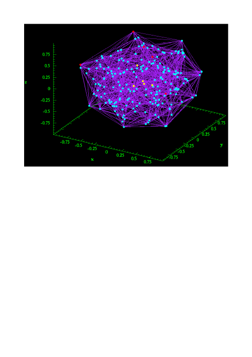
Figure 1: The geometrical domain of 1177 elements, formed from 202 nodes. The nodes are represented as cyan dots, except for the five that become the most saturated set (red) and the five that saturate least (yellow).

4.1 Nodal Solutions

Nodal solutions for the inversion were obtained by solving eq.(24) for the domain displayed in Fig. 1 for progressively increasing values of the model optical depth. Note that since the scalar distance $s$ is a common multiplier of all parts of $F_{p}^{j}$ in eq.(25), multiplication of these, or the node-summed $\Phi$ forms, by an extra scaling factor was sufficient to change the effective optical depth. After the first solution, where the initial guess at the fractional inversions was 1.0 for all nodes (unsaturated), initial guesses were based upon one or more previous solutions. Nodal solutions were eventually computed for optical depth multipliers between 0.5 and 13.5. These multipliers correspond to actual maximum maser depths that are approximately twice as large, as the dimensionless outer radius, rather than the diameter, of the original point distribution was 1.0. All successful solutions had a largest inversion residual smaller than 10^-8. Convergence problems eventually made progress to higher optical depth multipliers prohibitively slow beyond the upper limit of 13.5. However, it can be argued that the CVR approximation is already rather poor with the corresponding levels of saturation, and a switch to an approximation with weaker redistribution should be made.

To demonstrate the effects of increasing saturation (with optical depth) we show in Fig. 2 the inversions in the five most saturated, and the five least saturated, nodes as a function of the optical depth multiplier. The definitions of most and least saturated refer to the model at the highest optical depth achieved, as some swapping of the ordering with saturation does occur: for example, it is easy to see that Node 1, the least inverted node at maximum depth, does not become so until the depth multiplier reaches $\sim$8.5. Broadly speaking, the nodal inversions in Fig. 2 behave as expected. For the most saturated nodes, there is a rapid, almost linear, fall in the inversion with depth between depths of 7 and 10, followed by a distinct slowing of the saturation as the inversions fall below about 0.3. For the least-saturated set, all inversions remain above 0.9 over the range of depths investigated, and the phase of rapid population drop is only beginning beyond depths of $\sim$10.

Figure 2: The populations in the five most saturated nodes (lower panel) and the five least saturated nodes (upper panel) as a function of the optical depth multiplier.

Figure 3 shows the distribution of nodal inversions amongst decadal bins with increasing optical depth multiplier. All 202 inversions remained above 0.9 at a depth multiplier of 6.5; the first histogram plotted as at a depth of 8.5, where the great majority of nodes still have inversions $>$0.9. With increasing optical depth, an asymmetric distribution is built up, with the most populated bin moving to progressively lower inversions (rows 2 and 3 in Fig. 3).

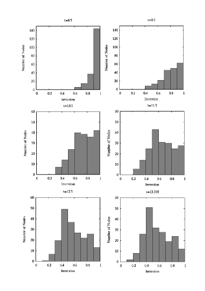
Figure 3: Histograms of the distribution of nodes amongst ten bins representing inversion ranges. Optical depth multipliers, $\tau$, marked at the top of each panel increase from left to right along each row, and by rows from top to bottom. Note the y-axis scale change in moving from the first to the second row.

The 0.9-1.0 bin ceases to be the most populated between $\tau=10.5$ and $\tau=11.5$, and at the latter depth, the most populated bin is clearly 0.5-0.6. A further shift to 0.4-0.5 has taken place by $\tau=12.5$.

Concentration of the least saturated nodes to the core of the domain, and most saturated nodes to the boundary, is demonstrated by taking the mean radii of the two groups of nodes displayed in Fig. 2: the mean radius of the five most saturated nodes is 0.9856, with a sample standard deviation of 0.0070, whilst the five least saturated nodes have a mean radius of only 0.2008 (sample standard deviation of 0.0736).

4.2 Formal Solutions

In the work discussed here, formal solutions were obtained by solving eq.(4) for a set of rays passing through the domain, with a known gain coefficient, based on known nodal inversions from eq.(5), and see Section 4.1 above. The nodal solutions can be for any optical depth multiplier, but in most of the work discussed here, they are for the maximum optical depth multiplier achieved. The rays for a formal solution originate on a disc that is larger than the maximum extent of the domain, and the disc was partitioned into zones for each ray as discussed in Section 3.3.1. Although the nodal solutions are for an undivided inversion, formal solutions were calculated for a number of spectral bins, or channels. The standard arrangement in this work allocated 25 spectral bins to cover 7 Doppler widths.

One of the expected observational features of a spherical, or near-spherical, maser cloud is that the apparent size of a cloud of fixed dimensions should diminish with increasing optical depth, a key beaming property discussed, for example, in Chapter 5 of Elitzur (1992). Testing this property is easy with the code in the current work, since the optical depth of a cloud of fixed dimensions is determined by a simple multiplier. We show in Fig. 4 the same view of the cloud at four different values of the optical depth multiplier. The observer’s position is along the $z$-axis of the model, at a scaled distance of $10^{4}$, so the observer is looking down on the North pole of the cloud from a distance vastly larger than the cloud dimensions, as shown by the $x$ and $y$ scales in the figure. The image is for the central spectral bin only. It is apparent that the emission of the cloud becomes increasingly centre brightened as the optical depth increases, so that the size of the object, down to, say, half the maximum brightness, falls as expected. Indeed the effect is more extreme than is apparent simply from the colour palette in Fig. 4 because the palette is re-scaled to a different range of numbers as the brightness range increases. While the background level is always 10^-5 with respect to the saturation intensity, the upper limit changes from 10^-3 at a depth multiplier of 2.0 to 10² in the later figures, where saturation becomes substantial. An observer with an interferometer of a fixed dynamic range of 10000 would therefore be able to see the object out to a radius of slightly more than 0.5 in the bottom right-hand panel, but would not detect the object at the depth of 2.0. The faint plume in the lower left corner of each panel in Fig. 4 is an artefact resulting from plotting the circular array of ray origins onto a square grid.

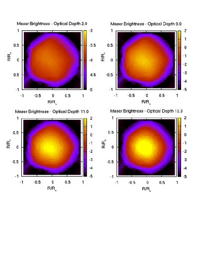
Figure 4: Simulated interferometer images of the cloud viewed from its North pole in the brightest (central) spectral channel. The value of the optical depth multiplier is shown for each image. On the distance scale shown, multiples of the model scale, $R_{m}$, the observer’s distance is $10^{4}$. Note that the figure in the top left, with the optical depth multiplier of 2.0, has a different colour scale to the other panels. In all cases the colour scale is proportional to the base-10 logarithm of the specific intensity divided by the saturation intensity.

In Fig. 5, we show the apparent size of the model maser feature as a function of the optical depth parameter for the line centre and two off-centre frequencies. The size here is defined as the fractional solid angle, or area, of the source that produces half the total flux as viewed by the observer, and is represented as the symbol $\Omega_{1/2}$. It is computed by generating partial fluxes from the brightest ray, in decreasing order, until half the total flux is reached. The solid angle corresponding to this subset of rays is then divided by the total solid angle of the source. The viewpoint and observer’s position are as used for Fig. 4 above.

Figure 5: The parameter $\Omega_{1/2}$ as a function of the optical depth multiplier for three dimensionless frequencies: 0.00, 0.84 and 1.70 Doppler widths from line centre. The parameter $\Omega_{1/2}$ is the fractional source area or solid angle that contributes half of the total flux at the observer’s position.

In this model, the apparent source size decreases monotonically with increasing maser depth at all frequencies. The smallest apparent size is found at line centre at all frequencies and, at any maser depth, the increase in size with frequency offset is monotonic. Saturation slows the decrease in apparent size with depth at all frequencies (see Fig. 5).

4.3 Simulations of Rotation

In order to study the possibility of flaring events with a single maser cloud, we have simulated observations of a rotating cloud by viewing a fixed cloud from a number of regularly spaced positions on a celestial great circle, centered on the cloud. Corrections were applied via the Doppler effect to convert between a rotating frame in which the cloud, assumed to be in solid-body rotation, is at rest, and the inertial frame of the observer. Further consequences of this arrangement with respect to the input radiation were avoided by assuming a spectrally flat background. If the rotation period, $P_{dec}$, is measured in decades, and the cloud diameter, $D_{AU}$, is in Astronomical Units, then the equatorial rotation velocity is

$$v_{rot}=1.49D_{AU}/P_{dec}\;\;\mathrm{km\,s^{-1}},$$ (26)

a value comparable to the speed of sound in the cloud gas.

With molecular velocities in the model scaled to a width parameter of $\bar{W}=\sqrt{2kT/m}$, where $T$ is the kinetic temperature and $m$ is the absolute molecular mass, rotation of a cloud of diameter $D$ with period $P$ leads to a maximum Doppler shift, from extreme red to line centre, of

$$\delta_{b}=4.14\frac{D_{AU}}{P_{dec}}\sqrt{\frac{m_{u}}{T_{100}}}$$ (27)

frequency bins, where 25 bins cover 7 Doppler widths (see Section 4.2). New quantites of order 1 in eq.(27) are the molecular mass in atomic mass units, $m_{u}$, and the kinetic temperature in units of 100 K, $T_{100}$. In the current work, a value of 1 was set for all these parameters, and a total of ten extra frequency bins assigned to allow for Doppler broadening, Five were allocated either side of the line centre, by rounding up the figure of 4.14 bins from eq.(27).

The greatest distance between any pair of boundary nodes of the domain was defined to be the long axis of the cloud. There are obviously an infinite number of unit vectors perpendicular to the long axis, but a rotation axis was chosen on the basis of the minimum absolute component algorithm. Having chosen this particular rotation axis, a set of observer’s positions were arranged in a plane that passed through the cloud origin perpendicular to the rotation axis. All observer’s positions were placed at a distance of $10^{4}$ in scaled units, as for the basic formal solutions. In the current work, 100 observer’s positions were used, equally spaced in angle around the plane defined above. Only one observer’s line of sight was exactly parallel to the long axis, and this occurred at a time of 0.3 yr. In the rotation models, the size of the source disc was based on the length of the long axis regardless of the observer’s position, so that the patch of sky viewed subtended the same solid angle in every case. This is unlike the ordinary formal solutions, where the size of the source disc is based on the maximum sky-plane extent of the cloud from the particular observer’s position.

Radiation transfer for the formal solutions, one per observer’s position, was carried out in the cloud frame, in which there can be no internal velocity gradients for solid-body rotation. The effects of the centrifugal and Coriolis frame forces were ignored, but their effects are discussed below in Section 4.3.2, regarding the stability of the cloud. Transformation to the observer’s frame was effected by calculating the perpendicular sky-plane distance of each ray from the rotation axis, and computing the associated Doppler shift in bins. Although the ray paths form a cone with the observer’s position at the apex, the observing positions are sufficiently distant, compared with the dimensions of the cloud, that convergence of rays through the cloud could be ignored, and the rays treated as parallel for the purposes of computing Doppler shifts.

The specific intensity of each ray was then shared between a pair of suitably shifted bins in proportion to the fractional overlap of the single bin of the old spectrum, and the new pair. The overall effect was mostly rotational broadening of the spectrum with a small (less than one bin) shift in the peak position at some observing positions. Overall, the Doppler corrected output radiation makes observing a fixed cloud from many observers’ positions analogous to observing a rotating cloud from a single position.

4.3.1 Results and Lightcurves

The basic results of the formal solutions simulating rotation are very similar to those of standard formal solutions: a table of specific intensities and a spectrum of flux densities for each rotation angle of the cloud. The major difference is that a maser light curve can be constructed by plotting suitable outputs as a function of rotation angle, or of time, based on a solid-body rotation speed.

There are, perhaps, three useful quantities that can be used on the $y$-axis of a light curve: one is the brightest specific intensity found in a table of size equal to the number of rays multiplied by the number of spectral bins. From an observer’s point of view, this would correspond to the brightest pixel in the image cube of a typical interferometric observation. The second possibility is the maximum flux density in the spectrum, regardless of the bin in which that maximum occurs. This quantity corresponds more to results seen by a single-dish observer. The third possibility is the total (frequency or velocity-integrated) flux. Light curves for all three of these quantities are plotted in Fig. 6 for a single rotation period of the cloud, 10 yr.

Figure 6: Normalized light curves for three possible observational quantities: $F_{pk}$ (solid line) is the maximum flux density in the spectrum; $I_{pk}$ (dashed line) is the brightest specific intensity, corresponding to the brightest pixel in an interferometer map at any channel; $F$ (dotted line) is the flux, integrated over all spectral channels. All quantities are normalized to the value at their own brightest epoch. Error bars, with half-height equal to the sample standard deviation, have been added for the integrated flux curve only for clarity. These standard deviations were computed from 1000 realizations with rotation axes that were also perpendicular to the long axis of the domain, but were otherwise of random orientation.

Perhaps the first point to note from Fig. 6 is that only $I_{pk}$, the brightest specific intensity, peaks at the time where the long axis is presented directly towards the observer. The maximum and integrated fluxes instead reach a maximum at 2 yr, and again, half a period later, at 7 yr. All three parameters, however, follow a similar pattern of four strong maxima per period in two pairs. As expected, the least averaged quantity, $I_{pk}$, displays the greatest dynamic range: the ratio between its first maximum and the deepest minimum, at 3.1 yr, is 2.94. A fainter maximum is visible at $\sim$4 yr, with a counterpart at 9 yr. Rise and fall times for all maxima are of the order of several months. The pattern of variability is continuous, with no distinct ‘on’ or ‘off’ states.

The curves plotted in Fig. 6 result from rotation about a specific axis that should not be special except that it was chosen to be perpendicular to the long axis of the domain. We therefore calculated dispersion information, based on 1000 realizations of the rotation model, each based on a different rotation axis. Each rotation axis was also on a circle perpendicular to the long axis, but the angle around this circle was chosen at random. The chosen dispersion statistic is the sample standard deviation, and error bars representing this have been plotted, for clarity, on the integrated flux curve only. The standard deviations for the other normalized quantities have similar behaviour, and are similar in magnitude, but somewhat larger, reflecting the less averaged quality of the peak flux and specific intensity. At times $t=0$ and $5$ yr, there are points with very small standard deviations, but once the observer’s position has moved well away from the long axis, typical standard deviations of 0.15-0.2 were found. This shows that, whilst the peaks near 0 and $5$ yr are always present due to orientation of the long axis close to the line of sight, other peaks and troughs are due only to the particular choice of the rotation axis. It should be noted, however, that for any given rotation axis, variability of a similar magnitude to that plotted in Fig. 6 is likely to be observed.

4.3.2 Stability of the Cloud

For any reasonable number density in a maser cloud, the cloud will be gravitationally stable. The Jeans length is of parsec scale, compared to the AU scale of the cloud. However, it is still useful to introduce the sound-crossing time, $t_{s}$, as a non-gravitational dynamical time, where

$$t_{s}=D/(2c_{s})=2.2D_{AU}(m_{u}/T_{100})^{1/2}\;\;\;{\rm yr},$$ (28)

and the sound speed $c_{s}=\sqrt{\gamma kT/m}$ has been used with the ratio of specific heats $\gamma=7/5$ for rigid diatomic molecules.

If the cloud is uniformly rotating, then, in the rotating frame of the cloud, the dominant forces acting on a parcel of gas at the surface of the cloud are the centrifugal frame force and the pressure difference between the cloud and any background medium in which the cloud is embedded. The equation of motion of the gas for an equatorial parcel of gas may be written,

$$\ddot{r}-\Omega^{2}r=-\beta,$$ (29)

where $\beta=\alpha n_{X}\sigma kT_{X}/m_{X}$ is a representation of the acceleration imparted by the pressure gradient, which has been written as $\alpha$ multiplied by the pressure of the external medium of number density, temperature and molecular mass, respectively $n_{X}$, $T_{X}$, $m_{X}$, acting over the mean-free-path $1/(\sigma n_{X})$, where sigma is the collision cross section. The general solution to eq.(29), if the initial radial velocity of the parcel of gas is zero, and the initial radius is the cloud radius, $R$, is

$$r(t)=(R-\beta/\Omega^{2})\cosh(\Omega t)+\beta/\Omega^{2}.$$ (30)

Two interesting extremes of eq.(30) are firstly the case of negligible external pressure ($\beta\sim 0$) in which case the cloud is unstable and disperses on a timescale of order $1/\Omega=P/(2\pi)$: for the cloud modelled in Fig. 6, approximately 1.6 yr. Secondly, in the case where $R-\beta/\Omega^{2}\ll 1$, the first term in eq.(30) can be ignored until some much larger time, and for times up to at least the order of $P$, the radius remains close to the constant value of $\beta/\Omega^{2}\sim R$. In the second case, the cloud is stable in the short term provided that $\alpha$ is small, that is the inward acceleration for centrifugal balance can be provided by only a small fraction of the pressure of the gas external to the cloud. With $\beta=R\Omega^{2}$, the value of $\alpha$ is

$$\alpha=\left(\frac{V_{rot}}{c_{sX}}\right)^{2}\frac{1}{R\sigma n_{X}}\simeq 7.3\times 10^{-4}\frac{D_{AU}}{P_{dec}^{2}T_{1000}\sigma_{20}n_{6}},$$ (31)

where $V_{rot}=\Omega R$ and $c_{sX}$ is the sound speed in the external gas. Other parameters are $T_{1000}$, the external gas temperature in units of 1000 K, $n_{6}$, the number density of the same material in units of $10^{6}$ cm^-3, and $\sigma_{20}$, the collision cross-section in units of $10^{-20}$ m². It does appear from eq.(31) that $\alpha$ will usually be small, allowing for a number of rotations before the cloud is destroyed.

Observational evidence from long-term single-dish monitoring of H₂O masers in massive star-forming regions (Lekht et al., 1999), suggests that, in a turbulence interpretation, there are either no long-lived vortices (which survive many rotations), or that the power spectrum of the turbulence is concentrated towards the largest scales. This in turn suggests that significant evolution in the shape of a cloud is likely in a single revolution, although identification of the model cloud with a turbulent eddy may not generally be appropriate. In evolved-stars, however, some maser structures supporting the 1612-MHz OH line survive for several pulsational cycles of typically 1 yr (Etoka & Le Squeren, 2000), and may therefore be long-lived if they are turbulence based.

4.4 Execution Times

Calculation of the nodal solutions dominates the execution time and, for the version of the code used in the present work, this is in turn dominated by the need to compute a Jacobian matrix of the derivatives of eq.(24) for the LM algorithm (see Section 3.3.1). The time needed to compute the Jacobian scales as the square of the number of nodes, whilst other calls to the solution checker scale only linearly. The time to complete one iteration of the Levenberg-Marquardt algorithm for the domain discussed in this work, call it $T$, is therefore approximately the time to compute the Jacobian, and it is equal to $\sim$270 s on an Intel Core i7-3930K CPU, rated at 3.20 GHz.

For values of the optical depth multiplier $\tau<$10, each solution requires an average of 2-3$T$, rising to $\sim$12$T$ when $\tau$ is in the approximate range 10-11.5. These estimates are based on a step of 0.1 in $\tau$ between solutions. This value of the step was used to give smooth results in graphs such as Fig. 2, and larger steps could have been used at small $\tau$. For values of $\tau>$11.5, progressively smaller step sizes must be used, and these became prohibitively small near the largest value of $\tau$ used in current work (13.303).

5 Discussion

There have been several previous essays at 3D-modelling of astrophysical masers, for example the toroidal model of hydrogen radio recombination-line masers in MWC349A (Báez-Rubio et al., 2013), and the protostellar (T-Tauri) disc model of methanol masers (Parfenov et al., 2016). However, the results presented in this paper are probably the first fully-3D maser solutions for an arbitrary degree of saturation. They span a range of stages from computation of inversions at each node of a triangulated domain, through the use of those solutions to carry out formal radiative transfer of rays from a background source to an observer, and the use of modified formal solutions to generate light-curves for a uniformly rotating maser cloud with Doppler rotational broadening.

Nodal solutions follow the expected pattern for an approximately spherical cloud, with the most saturated nodes found near the edges of the domain, and the least saturated nodes located near the centre. The brightest maser rays have intensities of approximately 600 times the saturation intensity in the most highly saturated version of the model. Formal solutions through a domain with known saturated nodal inversions leads to a clear reduction in the observed source size with increasing amplification and saturation. The effective source size, quantified as the source solid angle that provides half the observed flux, is clearly a function of frequency, and decreases monotonically with the degree of saturation at all frequencies. No effects such as the decrease in effective size with frequency for detunings smaller than approximately 1 Doppler width, as in Emmering & Watson (1994) were observed, but this is expected since the current work uses a CVR, rather than NVR, approximation for redistribution.

The light-curves show that very small deviations from spherical symmetry in a cloud supporting intense maser emission will result in significant changes in observed brightnesses, flux densities and fluxes. However, for cloud of similar shape to the one used here, the radiation beaming pattern is still far from the ideal filamentary type, even for the maximum depth parameter used. The contrast between minimum and maximum peak brightness for the rotation simulation is a factor of $\sim$3. Whilst this behaviour might be described as a small-amplitude flaring event, it can certainly not match the dynamic ranges of hundreds to thousands seen in, for example, extreme water-maser flares. Although the light-curves plotted in Fig. 6 are periodic, we would expect that geometrical evolution of the cloud would make variability from a real rotating cloud system only quasi-periodic. The dynamic ranges from the model light curve are more in accord with many of the flaring methanol sources monitored by Goedhart et al. (2004) over $\sim$4 yr. Two examples for comparison might be G331.13-024 (periodic) and G351.78-0.54 (aperiodic).

The numerical procedure used in this work has demonstrated that the integral equation method of solving the combined radiative transfer and inversion saturation problem is viable in 3-D finite element domains for strongly saturated maser sources. The method may be readily generalised to multi-level systems, weaker redistribution and non-uniform clouds. In the latter case, a more conventional numerical frequency integration is almost certainly better than the analytical technique used here, though under NVR this issue does not arise. A $J=1-0$ Zeeman polarization version of this model is under construction (Etoka & Gray, in preparation). For the more general multi-level case, we will work with fractional energy-level populations as the unknowns, and solve the set of statistical master equations for these populations. The coefficients of the master equations contain mean intensities that can be eliminated, as in the present work. However, in the general case, the mean intensity of a transition is replaced by a depth, solid angle and frequency integral over the pair of populations involved in the transition.

As noted in Section 4.4, performance of the code significantly degrades at values of the optical depth multiplier $>$11.5. This does not appear to be due to oscillation between multiple solutions of the non-linear equation problem, but instead appears to be due to an increasingly ‘shallow’ global minimum in the residuals. The fact that our strategy of starting from previous solutions at lower optical depth (see Section 3.3.1) is effective suggests that this is indeed the case. Improving the convergence properties of the code at high optical depths is obviously highly desirable. We have evidence that, as expected, increased resolution (more nodes) will do this, but at the expense of increased computing time. Other techniques that we intend to consider are better optimisation of the aspect ratios of the finite elements, better extrapolation algorithms than the current polint, and linear perturbation of eq.(24).

6 Conclusions

(1) Nodal inversion and formal RT solutions are as expected for a near-spherical maser; a discussion of historical apparent size versus frequency effects requires extension to an NVR model. (2) Rotation of the cloud provides a periodic signal of dynamic range approximately 3, purely from geometry, even for a domain that has only small departures from spherical symmetry. (3) On the grounds that a real cloud would likely evolve significantly during one rotation, this model cannot explain periodic flaring, but could produce quasi-periodic variability. (4) The domain used in the current work yields a light-curve that is not strongly weighted to either the higher or to the lower part of the flux range. It is therefore not a good model of sources with a very high, or very low, duty cycle.

Appendix A Analytic Frequency Integration

The standard power series expansion of the exponential in braces on the second line of eq.(15) leads to a general term, for power $n$ of the form

$$q_{n}=(1/n!)\left[\int_{\mn@boldsymbol{r}_{0}}^{\mn@boldsymbol{r}}d\mn@boldsymbol{r}^{\prime}\Delta(\mn@boldsymbol{r}^{\prime})\eta(\mn@boldsymbol{r}^{\prime})e^{-\eta^{2}(\mn@boldsymbol{r}^{\prime})(\tilde{\nu}-\hat{\mn@boldsymbol{n}}\cdot\mn@boldsymbol{u}(\mn@boldsymbol{r}^{\prime}))^{2}}\right]^{n}.$$ (32)

All such terms are subject to the frequency and solid angle integrals that appear in eq.(15). The power form of the expression in eq.(32) may be expanded to the multiple integral form,

$$q_{n} =(1/n!)\int_{\mn@boldsymbol{r}_{0}}^{\mn@boldsymbol{r}}d\mn@boldsymbol{r}_{n}\Delta(\mn@boldsymbol{r}_{n})\eta(\mn@boldsymbol{r}_{n})\int_{\mn@boldsymbol{r}_{0}}^{\mn@boldsymbol{r}}d\mn@boldsymbol{r}_{n-1}\Delta(\mn@boldsymbol{r}_{n-1})\eta(\mn@boldsymbol{r}_{n-1})...$$

$$...\int_{\mn@boldsymbol{r}_{0}}^{\mn@boldsymbol{r}}d\mn@boldsymbol{r}_{1}\Delta(\mn@boldsymbol{r}_{1})\eta(\mn@boldsymbol{r}_{1})\exp\left[-\sum_{k=1}^{n}\eta^{2}(\mn@boldsymbol{r}_{k})(\tilde{\nu}-\hat{\mn@boldsymbol{n}}\cdot\mn@boldsymbol{u}(\mn@boldsymbol{r}_{k}))^{2}\right],$$ (33)

noting that only the final exponential term is a function of frequency. The frequency integral from eq.(15) can therefore be brought inside all the spatial integrals in eq.(33) and written as,

$${\cal F}=\int_{-\infty}^{\infty}d\tilde{\nu}\exp\left[-\sum_{k=0}^{n}\eta^{2}(\mn@boldsymbol{r}_{k})(\tilde{\nu}-\hat{\mn@boldsymbol{n}}\cdot\mn@boldsymbol{u}(\mn@boldsymbol{r}_{k}))^{2}\right],$$ (34)

where $\mn@boldsymbol{r}_{0}=\mn@boldsymbol{r}$, the final position of the ray from eq.(15). The integral in eq.(34) can be carried out analytically in general via formula 7.4.32 from Abramowitz & Stegun (1972) with the coefficients $a=\sum_{k=0}^{n}\eta^{2}(\mn@boldsymbol{r}_{k})$ of the squared frequency, $b=-\sum_{k=0}^{n}\hat{\mn@boldsymbol{n}}\cdot\mn@boldsymbol{u}(\mn@boldsymbol{r}_{k})\eta^{2}(\mn@boldsymbol{r}_{k})$ of the frequency, and the frequency-independent term $c=\sum_{k=0}^{n}(\hat{\mn@boldsymbol{n}}\cdot\mn@boldsymbol{u}(\mn@boldsymbol{r}_{k}))^{2}\eta^{2}(\mn@boldsymbol{r}_{k})$. The result cannot generally be re-factored, but if there is no velocity field inside the cloud ($\mn@boldsymbol{u}=(0,0,0)$ everywhere), then $b=c=0$ and the result of eq.(34) is simply,

$${\cal F}=\left(\frac{\pi}{\sum_{k=0}^{n}\eta^{2}(\mn@boldsymbol{r}_{k})}\right)^{1/2}.$$ (35)

In the case of a uniform cloud, which will be assumed from now on, $\eta=1$ everywhere, and eq.(35) therefore reduces to ${\cal F}=\pi^{1/2}/\sqrt{(}n+1)$. This expression is a constant that can be removed from all the spatial integrals in eq.(33), leaving them in a form that is already factored, and can be restored to the power form in eq.(16) of the main text.

References

- Abraham et al. (1979) Abraham Z., Opher R., Raffaelli J. C., 1979, IAU Circular, 3415
- Abramowitz & Stegun (1972) Abramowitz M., Stegun I. A., 1972, Handbook of Mathematical Functions
- Alcock & Ross (1985) Alcock C., Ross R. R., 1985, ApJ, 290, 433
- Amini & Rostami (2015) Amini K., Rostami F., 2015, Journal of Computational and Applied Mathematics, 288, 341
- Anderson & Watson (1993) Anderson N., Watson W. D., 1993, ApJ, 407, 620
- Araya et al. (2007) Araya E., Hofner P., Sewiło M., Linz H., Kurtz S., Olmi L., Watson C., Churchwell E., 2007, ApJ, 654, L95
- Argon et al. (1993) Argon A. L., Greenhill L. J., Reid M. J., Moran J. M., Menten K. M., Henkel C., Inoue M., 1993, in American Astronomical Society Meeting Abstracts #182 Vol. 25 of Bulletin of the American Astronomical Society, First VLBI Observations of Extragalactic Water Vapor Maser Flares in IC10. p. 926
- Báez-Rubio et al. (2013) Báez-Rubio A., Martín-Pintado J., Thum C., Planesas P., 2013, A&A, 553, A45
- Beckers & Beckers (2012) Beckers B., Beckers P., 2012, Computational Geometry, 45, 275
- Bettwieser (1976) Bettwieser E., 1976, A&A, 50, 231
- Boboltz et al. (1998) Boboltz D. A., Simonetti J. H., Dennison B., Diamond P. J., Uphoff J. A., 1998, ApJ, 509, 256
- Brinch & Hogerheijde (2010) Brinch C., Hogerheijde M. R., 2010, A&A, 523, A25
- Cimerman (1979) Cimerman M., 1979, ApJ, 228, L79
- Daniel & Cernicharo (2013) Daniel F., Cernicharo J., 2013, A&A, 553, A70
- Elitzur (1990) Elitzur M., 1990, ApJ, 363, 638
- Elitzur (1992) Elitzur M., 1992, Astronomical masers. Kluwer, Dordrecht
- Elitzur & Asensio Ramos (2006) Elitzur M., Asensio Ramos A., 2006, MNRAS, 365, 779
- Emmering & Watson (1994) Emmering R. T., Watson W. D., 1994, ApJ, 424, 991
- Etoka & Le Squeren (1996) Etoka S., Le Squeren A. M., 1996, A&A, 315, 134
- Etoka & Le Squeren (2000) Etoka S., Le Squeren A. M., 2000, A&AS, 146, 179
- Goedhart et al. (2003) Goedhart S., Gaylard M. J., van der Walt D. J., 2003, MNRAS, 339, L33
- Goedhart et al. (2004) Goedhart S., Gaylard M. J., van der Walt D. J., 2004, MNRAS, 355, 553
- Goedhart et al. (2005) Goedhart S., Minier V., Gaylard M. J., van der Walt D. J., 2005, MNRAS, 356, 839
- Goldreich & Keeley (1972) Goldreich P., Keeley D. A., 1972, ApJ, 174, 517
- Gray (2012) Gray M. D., 2012, Maser Sources in Astrophysics. Cambridge University Press, Cambridge, UK
- King & Florance (1964) King J. I. F., Florance E. T., 1964, ApJ, 139, 397
- Lang & Bender (1973) Lang R., Bender P. L., 1973, ApJ, 180, 647
- Lekht et al. (1999) Lekht E. E., Mendoza-Torres J. E., Silant’ev N. A., 1999, Astronomy Reports, 43, 209
- Lekht & Sorochenko (1984) Lekht E. E., Sorochenko R. L., 1984, Soviet Astronomy Letters, 10, 307
- Litvak (1973) Litvak M. M., 1973, ApJ, 182, 711
- Madden et al. (1988) Madden S. C., Friberg P., Brown R., Godfrey P., 1988, IAU Circular, 4537, 1
- Neufeld (1992) Neufeld D. A., 1992, ApJ, 393, L37
- Ng (1974) Ng K.-C., 1974, J. Chem. Phys., 61, 2680
- Olson & Kunasz (1987) Olson G. L., Kunasz P. B., 1987, J. Quant. Spec. Rad. Trans., 38, 325
- Parfenov et al. (2016) Parfenov S. Y., Semenov D. A., Sobolev A. M., Gray M. D., 2016, MNRAS, 460, 2648
- Press et al. (1992) Press W. H., Teukolsky S. A., Vetterling W. T., Flannery B. P., 1992, Numerical recipes in FORTRAN. The art of scientific computing
- Rajabi & Houde (2017) Rajabi F., Houde M., 2017, Science Advances, 3, e1601858
- Scappaticci & Watson (1992) Scappaticci G. A., Watson W. D., 1992, ApJ, 387, L73
- Spaans & van Langevelde (1992) Spaans M., van Langevelde H. J., 1992, MNRAS, 258, 159
- Strelnitskii (1982) Strelnitskii V. S., 1982, Soviet Astronomy Letters, 8, 86
- Sugiyama et al. (2017) Sugiyama K., Nagase K., Yonekura Y., Momose M., Yasui Y., Saito Y., Motogi K., Honma M., Hachisuka K., Matsumoto N., Uchiyama M., Fujisawa K., 2017, PASJ, 69, 59
- Sullivan (1973) Sullivan III W. T., 1973, ApJS, 25, 393
- Szymczak et al. (2016) Szymczak M., Olech M., Wolak P., Bartkiewicz A., Gawroński M., 2016, MNRAS, 459, L56
- Watson & Wyld (2003) Watson W. D., Wyld H. W., 2003, ApJ, 598, 357
- Zienkiewicz & Taylor (2000) Zienkiewicz O., Taylor R., 2000, The Finite Element Method: The basis. Butterworth-Heinemann