Comparing the Behaviour of Deterministic and Stochastic Model of SIS Epidemic

Abstract

Studies about epidemic modelling have been conducted since before 19th century. Both deterministic and stochastiic model were used to capture the dynamic of infection in the population. The purpose of this project is to investigate the behaviour of the models when we set the basic reproduction number, $R_{0}$. This quantity is defined as the expected number of contacts made by a typical infective to susceptibles in the population. According to the epidemic threshold theory, when $R_{0}\leq 1$, minor epidemic occurs with probability one in both approaches, but when $R_{0}>1$, the deterministic and stochastic models have different interpretation. In the deterministic approach, major epidemic occurs with probability one when $R_{0}>1$ and predicts that the disease will settle down to an endemic equilibrium. Stochastic models, on the other hand, identify that the minor epidemic can possibly occur. If it does, then the epidemic will die out quickly. Moreover, if we let the population size be large and the major epidemic occurs, then it will take off and then reach the endemic level and move randomly around the deterministic’s equilibrium.

1 Introduction

Studies about epidemic modelling have been conducted since before 19th century. Both deterministic and stochastiic model were used to capture the dynamic of infection in the population. Upon the study, some other parameters were introduced to generalised the model, for example the infection and recovery rates, as well as if the infection occurs in close or open population.

One of the most important development in this study is threshold theorem. It states that an epidemic can only occur if the initial number of susceptibles is larger than some critical value which depends on the parameters of the model under consideration. The threshold behaviour is usually expressed in terms of epidemic basic reproduction number, $R_{0}$. This quantity is usually defined as the expected number of contacts made by a typical infective to susceptibles in the population. It is important to note that in general epidemic modelling, both stochastic and deterministic models have similar threshold value, which is attained at $R_{0}=1$.

According to Nåsell [15], the proportion of infectives in the deterministic model would converge to some equilibrium point as time approached infinity. There are only two stages of equilibrium, extinction or endemic. When $R_{0}$ below the threshold point, both deterministic and stochastic approaches have converged to extinction. Unfortunately, different outcome happens when $R_{0}$ exceed 1.

Motivation The main purpose of this paper is to investigate the behaviour of the SIS model when we set $R_{0}$. The model is named after the transition process, where each individual in the population is classified into some stages, i.e. susceptible (S) and infective (I). The characteristics of the model are also studied, especially the conditions when the models enter the endemic- equilibrium level.

2 The SIS Epidemic Model

Suppose that we have a closed mixing population with initially $n$ individuals and $m$ infectives, where $m<<n$. We define the SIS model as follows.

At $t=0$, there are $n-m$ susceptibles who are vulnerable to the diseases. Each infective contacts each susceptible according to independent Poisson processes with rate $\lambda/n$ and if a susceptible is contacted, it immediately becomes an infective. The infectives also have an infectious period which follow iid exponential distributions with rate $\gamma$, and then removed, but once the infective’s infectious period is over, the individual will immediately become vulnerable to the disease. Finally, the epidemic ends when no infective is left in the population. The transition scheme of this model is illustrated in figure 1.

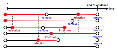
Figure 1: SIS epidemic illustration

2.1 The Transition Schemes of SIS Model

In this paper, we will assume that the population is closed. According to the figure 1, the SIS model consists of two processes, i.e. infection and removal.

For $t\geq 0$, let $Y_{n}(t)$ be the number of infectives at time $t$. Suppose that $Y_{n}(t)=i$, where $i\in\{1,2,\ldots n-1\}$. Then, there are $(n-i)i$ contacts between infectivees and susceptibles in the population. Therefore, the probability of infection and removal occurence in interval $(t,t+dt)$ are respectively

$$\mathbb{P}\{Y_{n}(t+dt)=i+1|Y_{n}(t)=i\} =\lambda/n\cdot(n-i)i\cdot dt+o(dt),$$ (1)

$$\mathbb{P}\{Y_{n}(t+dt)=i-1|Y_{n}(t)=i\} =\gamma i\cdot dt+o(dt).$$ (2)

2.2 The Deterministic Approach of SIS Model

To capture the behaviour of the SIS model, suppose that we allow $Y_{n}(t)$ be non–integer. Considering there are two transisitions in the model, we can interpret the transition scheme as follows

$$Y_{n}(t+dt)=Y_{n}(t)+\left(\frac{\displaystyle\lambda}{\displaystyle n}Y_{n}(t)\left[n-Y_{n}(t)\right]-\gamma Y_{n}(t)\right)dt+o(dt)$$ (3)

which yields as $dt\rightarrow 0$,

$$\frac{\displaystyle dY_{n}(t)}{\displaystyle dt}=\frac{\displaystyle\lambda}{\displaystyle n}Y_{n}(t)\left[n-Y_{n}(t)\right]-\gamma Y_{n}(t).$$ (4)

Let $y(t)=\frac{\displaystyle Y_{n}(t)}{\displaystyle n}$ represent the proportion of infective in the population at time $t$, then we can scale equation (3) as

$$\frac{dy(t)}{dt} =\lambda y(t)\cdot(1-y(t))-\gamma y(t),$$ (5)

where $\lambda y(t)\cdot(1-y(t))$ and $\gamma y(t)$ are infection and removal rate transitions of $y(t)$ with solution

$$y(t)=\begin{cases}\frac{\displaystyle(\lambda-\gamma)y(0)\cdot e^{(\lambda-\gamma)t}}{\displaystyle\lambda-\gamma+\lambda y(0)\left(e^{(\lambda-\gamma)t}-1\right)}&\text{if }\lambda\neq\gamma,\\ \frac{\displaystyle y(0)}{\displaystyle 1+\lambda y(0)t}&\text{if }\lambda=\gamma.\end{cases}$$

Figure 5 showed the behaviour of the processes with initial $(n,m)=(100,20)$. The stochastic processes behaved similar to deterministic models, but in other figures, some stochastic processes were not mimicing the behaviour of deterministic model, especially when $R_{0}>1$.

From the simulations, there are some tentative conditions that can distinguish the behaviour of deterministic and stochastic approaches to model SIS. These conditions are determined by the value of $R_{0}$, as the threshold theorem stated:

1. both deterministic and stochastic approaches of SIS will go exinct if and only if $R_{0}\leq 1$,

2. in deterministic approach, as $t\rightarrow\infty$, the SIS model showed an outbreak of disease as $R_{0}>1$,

3. in stochastic approach, there are two possibility of outcomes when $R_{0}>1$, i.e. the outbreak as deterministic approach or an extinction.

Therefore, we will prove mathematically the three points above to determine the behaviour of SIS model based on its reproduction number.

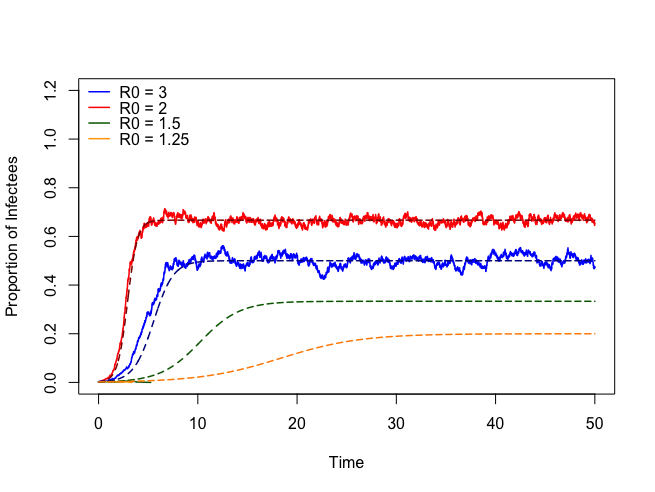
Figure 2: Initial susceptibles $=998$

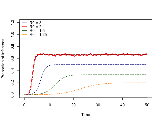
Figure 3: Initial susceptibles $=2998$

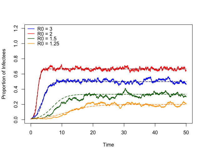
Figure 4: $(S_{0},I_{0})=(990,10)$

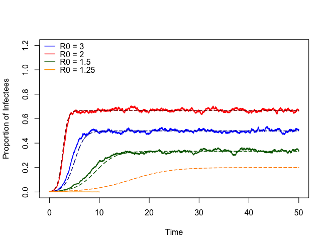
Figure 5: $(S_{0},I_{0})=(2990,10)$

3 The Behaviour of SIS Model According to Deterministic Approach

Recall equation (5). Obviously, the major epidemic occurs if and only if $\frac{\displaystyle dy}{\displaystyle dt}>0$ and otherwise. At some time $t,$ the increment of $y(t)$ will reach stationary and the process will hit the equilibrium point as shown in Figure 5 to 5. The roots of $\frac{\displaystyle dy}{\displaystyle dt}=0,$ are $y(t)=0$ when $R_{0}=\lambda/\gamma\leq 1$ and $y(t)=1-R_{0}^{-1}$ when $R_{0}$ exceeds 1. Therefore, according to the deterministic approach, the outbreak of epidemic happens when $R_{0}$ exceeds 1 with probability one, and otherwise.

4 The Behaviour of SIS Model According to Stochastic Approach

It is easier to study stochastic model of SIS using simulation. In deterministic approach, minor epidemic occurs if and only if $R_{0}\leq 1$, whilst major epidemic occurs otherwise. This is because when we let $\frac{\displaystyle dy}{\displaystyle dt}\leq 0\left(\text{or }\frac{\displaystyle dy}{\displaystyle dt}>0\right)$, the proportion of infection in (5) decreases (increases) in population upon time $t$ and then, the process will reach equilibrium.

As $t\rightarrow\infty$, the stochastic model of SIS also behaved in similar way. In fact, some processes will mimic the deterministic model, but others are not. In the next section, we will mathematically show why and what conditions stochastic model mimicing deterministic model.

4.1 Density Dependence Population Process

Suppose that $\{\boldsymbol{X}_{n}(t):t\geq 0\}$ is the CTMC process defined on $d$-dimensional integer lattice $\mathbb{Z}^{d}$ with finite number of possible transitions, given by $q_{i,i+l}=n\beta_{l}\left(\frac{\displaystyle k}{\displaystyle n}\right)$ where we define

$$\beta_{l}:\mathbb{Z}^{d}\rightarrow\left[0,\infty\right),l\in\Delta\subseteq\mathbb{Z}^{d},\sum_{l}\beta_{l}\left(\boldsymbol{x}\right)<\infty$$

for all $\boldsymbol{x}\in\mathbb{Z}^{d}$.

According to Ethier and Kurtz [10], if the the size of a certain population was $k$, then the density of that population was $\frac{\displaystyle k}{\displaystyle n}$ with intensities approximated proportionally to its size. For example, suppose that there are $i$-susceptibles and $j$-infectious individuals. The infectious and removal rates are given in eq. (1) and (2), which are density–dependent functions.

Suppose that $Y_{l}$ is a independent standard Poisson process, where each of possible transition $l\in\Delta$. By letting $\boldsymbol{X}_{n}(0)$ be non-random,

$$\boldsymbol{X}_{n}(t)=\boldsymbol{X}_{n}(0)+\sum_{l}lY_{l}\left(n\int_{0}^{t}\beta_{l}\left(\frac{\displaystyle\boldsymbol{X}_{n}(s)}{\displaystyle n}\right)ds\right).$$ (6)

Now let $\tilde{Y}_{l}(u)=Y_{l}(u)-u$ be a centered Poisson process at its expectation and $\boldsymbol{\bar{X}}_{n}(t)=\displaystyle\frac{\boldsymbol{X}_{n}(t)}{n}$. Following equation (6) and letting $F(\boldsymbol{x})=\displaystyle\sum_{l\in\Delta}l\beta_{l}(\boldsymbol{x})$,

$$\boldsymbol{\bar{X}}_{n}(t) =\bar{\boldsymbol{X}}_{n}(0)+\frac{1}{n}\sum_{l\in\Delta}l\tilde{Y}_{l}\left(n\int_{0}^{t}\beta_{l}\left(\bar{\boldsymbol{X}}_{n}(s)\right)ds\right)+\int_{0}^{t}F(\bar{\boldsymbol{X}}_{n}(s))ds.$$ (7)

We will show that the stochastic process in equation (7) can be approximated by non-random quantity when we let the population size become sufficiently large. But before that, consider following theorem.

Theorem 4.1.

If $\{Y(t),t\geq 0\}$ is a standard Poisson process, then for all $s\leq t$,

$$\lim_{n\rightarrow\infty}\sup_{s\leq t}\mid n^{-1}Y(ns)-s\mid=0$$

almost surely.

Proof.

Note that $Y(ns)\sim\text{Poisson}(ns)$, for $s\geq 0$. We can show easily show that $(Y(ns)-ns)^{4}$ is a submartingale. Therefore, for any $\varepsilon>0$

$$P\left(\sup_{0\leq s\leq t}\left|Y(ns)-ns\right|\geq\varepsilon n\right) =P\left(\sup_{0\leq s\leq t}(Y(ns)-ns)^{4}\geq\varepsilon^{4}n^{4}\right)$$

$$\leq\frac{E(Y(nt)-nt)^{4}}{\varepsilon^{4}n^{4}}=\frac{nt(1+3nt)}{\varepsilon^{4}n^{2}}\leq\frac{C(\varepsilon,t)}{n}.$$ (8)

If we let $n\rightarrow\infty$, then $P\left(\displaystyle\sup_{0\leq s\leq t}\left|Y(ns)-ns\right|\geq\varepsilon n\right)\rightarrow 0$. It implies that $\sum_{n=1}^{\infty}P\left(\left|Y(ns)-ns\right|\right)<\infty$ since the probability of its supremum tends to zero as $n\rightarrow\infty$. Therefore, according to Borel– Cantelli Lemma, $\displaystyle\lim_{n\rightarrow\infty}\sup_{s\leq t}\mid n^{-1}Y(ns)-s\mid=0$ almost surely. ∎

Now we will prove that eq. (7) can be approximated by non–random quantity as $n\rightarrow\infty$ by proofing theorem below.

Theorem 4.2.

Let $\displaystyle\lim_{n\rightarrow\infty}\bar{X}_{n}(0)=x_{0}$ and $x(t)=x_{0}+\displaystyle\int_{0}^{t}F(x(u))du$ be the deterministic version of equation (7). Suppose that for each compact $K\subset\mathbb{R}^{d},\exists M_{K}>0$ such that $\forall x,y\in K,\quad\mid F(x)-F(y)\mid\leq M_{K}\mid x-y\mid.$ Then, for $0\leq s\leq t,$

$$\lim_{n\rightarrow\infty}\sup_{s\leq t}\mid\bar{X}_{n}(s)-x(s)\mid=0$$

almost surely.

Proof.

Given $x(t)=x_{0}+\displaystyle\int_{0}^{t}F(x(u))du$, thus

$$\mid\bar{X}_{n}(t)-x(t)\mid \leq\mid\bar{X}_{n}(0)-x(0)\mid+\frac{1}{n}\sum_{l\in\Delta}\mid l\mid\sup_{s\leq t}\mid\tilde{Y}_{l}\left(n\beta_{l}\left(\bar{X}_{n}(s)\right)\right)\mid+\int_{0}^{t}M_{k}\mid\bar{X}_{n}(s)-x(s)\mid ds.$$ (9)

Now consider the second term of the right hand side of equation (9).

$$\frac{1}{n}\sum_{l\in\Delta}\mid l\mid\cdot\sup_{s\leq t}\mid\tilde{Y}_{l}\left(n\beta_{l}\left(\bar{X}_{n}(s)\right)\right)\mid =\sum_{l\in\Delta}\mid l\mid\cdot\sup_{s\leq t}\mid n^{-1}Y_{l}\left(n\beta_{l}\left(\bar{X}_{n}(t)\right)\right)-\beta_{l}\left(\bar{X}_{n}(t)\right)\mid.$$

According to Theorem 4.1, as $n\rightarrow\infty$, $\mid n^{-1}Y_{l}\left(n\beta_{l}\left(\bar{X}_{n}(t)\right)\right)-\beta_{l}\left(\bar{X}_{n}(t)\right)\mid\rightarrow 0$ almost surely. Therefore, equation (9) now becomes

$$\mid\bar{X}_{n}(t)-x(t)\mid =\mid\bar{X}_{n}(0)-x(0)\mid+\int_{0}^{t}M_{k}\mid\bar{X}_{n}(s)-x(s)\mid ds$$

$$\leq\mid\bar{X}_{n}(0)-x(0)\mid\cdot e^{M_{K}t}=0$$ (10)

by Gronwall’s inequallity. Therefore, by sanwich property, $\displaystyle\lim_{n\rightarrow\infty}\displaystyle\sup_{s\leq t}\mid\bar{X}_{n}(s)-x(s)\mid=0.$ ∎

Theorem 4.2 suggests that as $n\rightarrow\infty$, the process $\{\bar{\boldsymbol{X}}_{n}(t),t\geq 0\}$ will resemble the deterministic version $\boldsymbol{x}(t)$. If $\{Y_{n}(t),t\geq 0\}$ represents the number of infectees at time $t$ in SIS epidemic, then as $n$ sufficiently large and $t\rightarrow\infty$, the process will settle down and randomly move around its mean, in this case are the equilibrium points of deterministic model.

4.2 Branching Process

The mimicing behaviour of stochastic model of SIS is due to the convergence of its process, where according to the density dependent population process, as $n\rightarrow\infty$ the tail of stochastic model of SIS will converge to its mean. Note that after reaching some time, deterministic model of SIS will reach its stationary stage, i.e, extinction or endemic, which actually are the mean of stochastic SIS model.

According to Theorem 4.2, all stochastic processes of SIS should be mimicing the deterministic model. Obviously if $R_{0}\leq 1$, both stochastic and deterministic models go to extinction. Unfortunately, when $R_{0}$ exceeds 1, there are some cases when stochastic model extincts. These are illustrated in Figure 5 and 5. In stochastic processes, this anomaly is not surpraising at all since given a small number of infectees in an early epidemic, there is non–zero chance that the individual will recover before it makes contact to any susceptibles. The best analogy to illustrate this scenario is by branching process theorem.

Suppose that in a closed population, just by the end of its lifetime, each individual has independently produced $j\geq 0$ offsprings with probability $P_{j}$. Let $X_{n}$ denote the size of $n$-th generation, then the process $\{X_{n}:n=0,1,2,\cdots\}$ is a Markov chain having non-negative integer state space, where state $0$ is a recurrent state and others are transient. Since any finite transient state will be visited finitely often, this leads to the conclusion that if $P_{j}>0$, then the population will either die out or take off.

Let $\mu$ be the mean number of offspring from a single individual, then

$$E(X_{n}) =E\left(E\left(\sum_{j=1}^{X_{n-1}}\zeta_{j}\mid X_{n-1}\right)\right),\quad\zeta_{j}\text{ is number of $j$th individual's offspring}$$

$$=\mu^{2}E(X_{n-2})=\cdots=\mu^{n}E(X_{0})=\mu^{n},\quad\text{given $X_{0}=1$}.$$

Suppose that $\pi_{0}=\displaystyle\lim_{n\to\infty}P(X_{n}=0|X_{0}=1)$ denotes the probability that the population dies out. Note that if $\mu<1$, then $P(X_{n}\geq 1)\rightarrow 0$ almost surely as $n\rightarrow\infty$. This concept is very useful in epidemic modelling because when the expected number of infection is less than $1$, then the epidemic will obviously die out. But, if $\mu>1$, by conditioning on the $X_{1}$, $\pi_{0}=\sum_{j=0}^{\infty}P(\text{population dies out}|X_{1}=j)P_{j}.$

Note that given $X_{1}=j$, the population will eventually die out if and only if each of the $j$ families started by the members of the first generation die out. This statement is supported by the fact that the probability of extinction occuring in the early stage is non-zero. Moreover, the probability that the members of a typical family to die out is $\pi_{0}$. Thus, assuming that each individual acts independently, $P(\text{population dies out}|X_{1}=j)=\pi_{0}^{j}.$

Hence, $\pi_{0}$ must satisfy

$$\pi_{0}=\sum_{j=0}^{\infty}\pi_{0}^{j}P_{j}=E\left(\pi_{0}^{X_{1}}\right)=f(\pi_{0})$$ (11)

where $f(\pi_{0})$ is the pgf (probability generating function) of $X_{1}$, in such a way that $\pi_{0}$ is the smallest root in $[0,1]$ satisfying equation (11).

Table 1: Comparison table of probability the epidemics to die out approximated by branching process and empirical with $m=1$

$R_{0}$	Population Size	Branching Process	Empiral (10000 runs)
$\leq 1$	$N=100$	$1$	$1$
	$N=1000$	$1$	$1$
3.0	$N=100$	$0.3333$	$0.3420$
	$N=1000$	$0.3333$	$0.3331$
5.0	$N=100$	$0.2$	$0.1997$
	$N=1000$	$0.2$	$0.1996$
8.0	$N=100$	$0.125$	$0.1273$
	$N=1000$	$0.125$	$0.1282$

Now suppose that $T_{i}$ is infection period of $i$-th typical infective, which is assumed to follow independent exponential distributions with intensity $\gamma$ and let $R$ be the total number of contacts made by a typical infective in the epidemic model. Then,

$$R\mid T=t \sim\text{Poisson}(\beta t)$$ (12a)

$$T \sim\text{exponential}(\gamma).$$ (12b)

Now, suppose that $f(s),s\in[0,1]$ is the pgf of $R$ and $g(t)\quad(t\geq 0)$ is the pdf of $T$. Then,

$$f(s) =\sum_{k=0}^{\infty}s^{k}\int_{0}^{\infty}P(R=k\mid T=t)g(t)dt=\frac{\gamma}{\beta+\gamma}\sum_{k=0}^{\infty}\left(\frac{s\beta}{\beta+\gamma}\right)^{k}.$$

We find $s$, such that $f(s)=s$. Therefore, $s=1\quad\text{or}\quad s=\frac{\gamma}{\beta}.$ If $\gamma\geq\beta$, then the smallest root is $1$, but if $\gamma<\beta$, then the smallest root is $\frac{\displaystyle\gamma}{\displaystyle\beta}$. Hence, suppose there are $m$ initial infectives in the population and assuming that the contacts made are mutually independent, then

$$P(\text{epidemic dies out})\approx\begin{cases}1&\text{if }\gamma\geq\beta\\ \left(\frac{\displaystyle\gamma}{\displaystyle\beta}\right)^{m}&\text{if }\gamma<\beta.\end{cases}$$

Once again, the above result explains threshold behaviour of the process. All figures confirm the interpretation of threshold behaviour of the SIS deterministic model, that if $R_{0}>1$, major epidemic will occur despite of its initial values and population size. But in the stochastic model (which are displayed in jagged plots), some plots do not mimic the deterministic paths. Another simulation is provided in Table 1, where we compare the probability of the epidemics to die out approximated by brancing process and empirical.

5 Conclusion

We have successfully showed that both deterministic and stochastic models performed similar results when $R_{0}\leq 1$. That is, the disease-free stage in the epidemic. But when $R_{0}>1$, the deterministic and stochastic approaches had different interpretations. In the deterministic models, both the SIS and SIR models showed an outbreak of the disease and after some time $t$, the disease persisted and reached endemic-equilibrium stage. The stochastic models, on the other hands, had different interpretations. If we let the population size be sufficiently large, the epidemic might die out or survive. There were essentially two stages to this model. First, the infection might die out in the first cycle. If it did, then it would happen very quickly, just like the branching process theory described. Second, if it survived the first cycle, the outbreak was likely to occur, but after some time $t$, it would reach equilibrium just like the deterministic version. In fact, the stochastic models would mimic the deterministic’s paths and be scattered randomly around their equilibrium point.

6 Reference

References

- [1] H. Andersson and B. Djehiche, “A Threshold Limit Theorem for the Stochastic Logistic Epidemic”, J. Appl. Prob. 35, 662–670 (1998).
- [2] N. T. Bailey, The Mathematical Theory of Infectious Diseases and its Applications, 2nd edition (Griffin, London, 1975).
- [3] F. G. Ball, “The Threshold Behaviour of Epidemic Models”, J. Appl. Prob. 20, 227–241 (1983).
- [4] F. G. Ball, Epidemic Thresholds. Encyclopedia of Biostatistics. 3. (John Wiley & Sons, Chichester, 1998).
- [5] P. G. Ballard, N. G. Bean, J. V. Ross, “The Probability of Epidemic Fade-Out is Non-Monotonic in Transmission Rate for Markovian SIR Model with Demography”, Submitted J. Theoretical Bio. 393, 170–178 (2016).
- [6] H. Andersson and T. Britton, Stochastic Epidemic Models and Their Statistical Analysis (Springer, New York, 2000).
- [7] D. Clancy and P. K. Pollett, “A Note on Quasi-Stationary Distributions of Birth-Death Processes and the SIS Logistic Epidemic”, Submitted J. Appl. Prob. 40, 821–825 (2003).
- [8] J.N. Darroch and E. Seneta, “On Quasy-Stationary Distributions in Absorbing Discrete-Time Finite Markov Chains”, Submitted J. Appl. Prob. 2, 88–100 (1965).
- [9] J.N. Darroch and E. Seneta, “On Quasy-Stationary Distributions in Absorbing Continuous-Time Finite Markov Chains”, Submitted J. Appl. Prob. 4, 192–196 (1967).
- [10] S. N. Ethier and T. G. Kurtz, Markov Processes Characterization and Convergence (Wiley, New York, 1982).
- [11] s.‘Karlin, A First Course in Stochastic Processes. 2nd ed. (Academic Press Inc., California, 1975).
- [12] F. P. Kelly, Reversibility and Stochastic Networks (Cambridge University Press, Cambridge, 2011).
- [13] D. G. Kendall, “On the Generalized Birth and Death Process”, The Annals of Mathematical Statistics 19, 1–15 (1948).
- [14] R. J. Kryscio and C. Lefévre, “On the Extinction of SIS Stochastic Logistic Epidemic”, J. Appl. Prob. 26, 685–694 (1989).
- [15] I. Nåsell, “Stochastic Models of Some Endemic Infections”, Math. Bioscie. 179, 1–19 (2002).
- [16] R.H. Norden, “On the Distribution of The Time to Extinction in the Stochastic Logistic Population Model”, Adv. in Appl. Prob. 14, 687–708 (1982).
- [17] S.M. Ross, Introduction to Probability Models. 9th ed. (Elsevier Inc., London, 2007).
- [18] K. Susvitasari, “The Stochastic Modelling on SIS Epidemic Modelling”, Journal of Physics: Conference Series 795 (2017).