Stochastic Model of SIR Epidemic Modelling

Abstract

Threshold theorem is probably the most important development of mathematical epidemic modelling. Unfortunately, some models may not behave according to the threshold. In this paper, we will focus on the final outcome of SIR model with demography. The behaviour of the model approached by deteministic and stochastic models will be introduced, mainly using simulations. Furthermore, we will also investigate the dynamic of susceptibles in population in absence of infective. We have successfully showed that both deterministic and stochastic models performed similar results when $R_{0}\leq 1$. That is, the disease-free stage in the epidemic. But when $R_{0}>1$, the deterministic and stochastic approaches had different interpretations.

1 Introduction

In epidemic modelling, the deterministic and stochastic approximations were use to model the behaviour, especially to know the final outcome of the epidemic. Both models were important in any sense to describe this behaviour process. The deterministic model, in fact, is also an approximation of the stochastic model when the population size is sufficiently large.

Threshold theorem is the most important occurence in the development of the mathematical theory of epidemic. The threshold behaviour is usually expressed in term of epidemic basic reproduction number, $R_{0}$. This quantity is usually defined as the expected number of contacts made by a typical infectious individual to any susceptibles in the population. It is important to note that in general epidemic modelling, both stochastic and deterministic models have similar threshold value, which is attained at $R_{0}=1$. It then turns out that the models identify two parameter regions, $R_{0}\leq 1$ and $R_{0}>1$, with qualitatively different behaviour. In the deterministic model, minor epidemic always occurs if $R_{0}\leq 1$ with probability one, otherwise the major epidemic occurs also with probability one. So, the deterministic model simply identifies the process behaviour according to the value of $R_{0}$. But in the stochastic model, if we let the size of population be sufficiently large, minor epidemic definitely occurs when $R_{0}\leq 1$, whilst when $R_{0}>1$ major epidemic occurs with probability $p\in(0,1)$. It means that there is non-zero probability that the epidemic will die out even though $R_{0}>1$. This is an important difference between the two approaches.

In this paper, we will focus on the stochastic behaviour of the SIR epidemic model. Unlike SIS, we model SIR using the 2–dimensional Markov chain. We will also consider an SIR model with demography. Tabel 1 represents the transition rates of the SIR model in this paper.

Table 1: Transition rates of SIR model with demography

Description	Transitions	Rates
birth of susceptibles	$(S,I,R)\rightarrow(S+1,I,R)$	$\mu n$
death of susceptibles	$(S,I,R)\rightarrow(S-1,I,R)$	$\mu S$
death of infectives	$(S,I,R)\rightarrow(S,I-1,R)$	$\mu I$
death of removed	$(S,I,R)\rightarrow(S,I,R-1)$	$\mu R$
infection	$(S,I,R)\rightarrow(S-1,I+1,R)$	$\lambda SI/n$
removal	$(S,I,R)\rightarrow(S,I-1,R+1)$	$\gamma I$

We define a fixed birth rate of susceptibles, $\mu n$, and death rates of susceptible, infectious, and immuned individuals as $\mu S,\mu I,\mu R$. In contrast with model without demography, according to Nåsell [12], the SIR model with demography admits an almost stationary behaviour, corresponding to endemic infectious. Furthermore, we will also investigate the dynamic of susceptibles in population in absence of infective.

2 The SIR Model with Demography

In the model with demography, the population size is not closed, but actually depends upon the size of $S,I,\text{ and }R$ at time $t$. But in this case, since the birth rate of susceptibles is constant $\mu n$, the dynamical number of population due to the death rates will hardly affect the population size. Therefore, it is enough to only track the size of susceptibles and infectious individuals only.

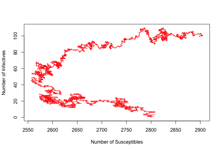
(a) Susceptibles vs infectives plot.

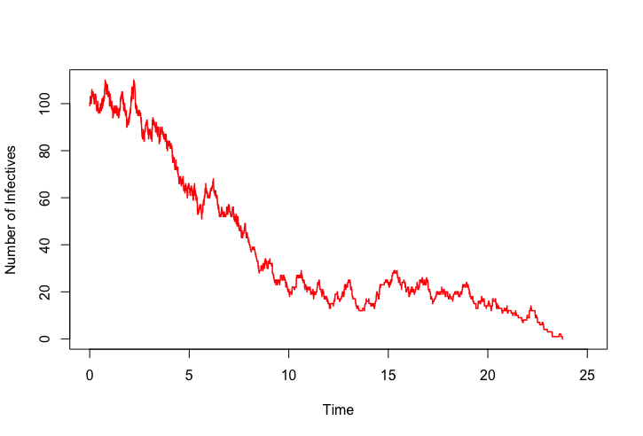
(b) Infectives vs time plot.

Figure 1: SIR with demography with $(R_{0},\mu,\gamma)=(1,0.1,1)$ and $(S(0),I(0))=(2900,100)$

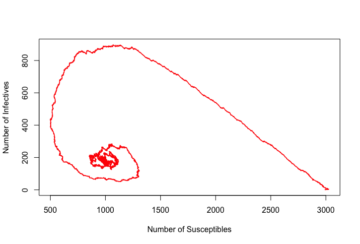
(a) $R_{0}=3$.

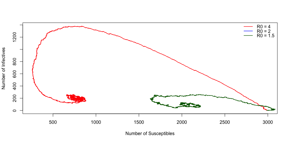
(b) $R_{0}=4,2,1.5$.

Figure 2: SIR with demography with $(\mu,\gamma)=(0.1,1)$ and $(S(0),I(0))=(2999,1)$

Similar to SIS model, SIR model also has threshold at $R_{0}=1$. In Figure 1, the epidemic dies out even though we assign quite a large number of initial infectious individuals, but in Figure 2aa, the epidemic takes off and survives in the first cycle. Another interesting fact is shown in Figure 2bb, one sample dies out quickly even though $R_{0}=2>1$. The normal scenario is that epidemic will die out if and only if $R_{0}\leq 1$, and take off otherwise due to eq.(1a) and (1b). But an anomaly occurs, which cannot explained by the deteministic model. There is a non–zero probability that the SIR will die out even though $R_{0}>1$.

2.1 The Deterministic Model of SIR with Demography

We define the SIR model using 2–dimensional Markov chain process. Suppose the process $\{(X_{n}(t),Y_{n}(t)):t\geq 0\}$ be the number of susceptibles and infectious individuals at time $t$, given inially size $n$ population.

The transition schemes of SIR model with demography is as follows

$$\frac{dX_{n}(t)}{dt} =\mu\left(n-X_{n}(t)\right)-\frac{\lambda}{n}X_{n}(t)Y_{n}(t)$$ (1a)

$$\frac{dY_{n}(t)}{dt} =\frac{\lambda}{n}X_{n}(t)Y_{n}(t)-(\mu+\gamma)Y_{n}(t).$$ (1b)

Suppose that $x(t)=\frac{\displaystyle X_{n}(t)}{\displaystyle n}$ and $y(t)=\frac{\displaystyle Y_{n}(t)}{\displaystyle n}$ denote the proportion of number of susceptibles and infectives at time $t$ respectively. Then, we can scale eq. (1a) and (1b) as follows

$$\frac{dx(t)}{dt} =\mu\left(1-x(t)\right)-\lambda x(t)y(t)$$ (2a)

$$\frac{dy(t)}{dt} =\lambda x(t)y(t)-(\mu+\gamma)y(t).$$ (2b)

Now we are interested to find the equilibrium points of the eq. (2a) and (2b). Setting $\displaystyle\frac{dx(t)}{dt}=0$ and $\displaystyle\frac{dy(t)}{dt}=0$ yields two equilibrium points. Suppose that $R_{0}=\displaystyle\frac{\lambda}{\mu+\gamma}$, equilibrium point $(1,0)$ is attained if and only if $R_{0}\leq 1$, and $\left(R_{0}^{-1},\displaystyle\frac{\mu}{\mu+\gamma}-\frac{\mu}{\lambda}\right)$ if and only if $R_{0}>1$. Using Theorem 4.1 in [14], the stochastoc process will mimic the behaviour of the deterministic process as $t\rightarrow\infty$ (see Figure 3).

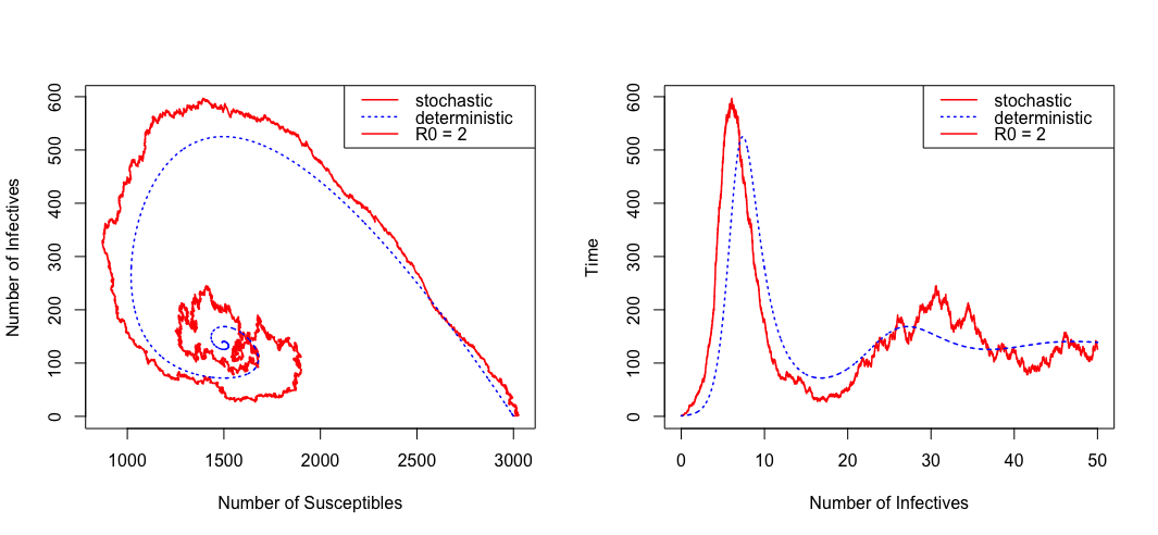
Figure 3: SIR epidemic with parameter $(R_{0},\mu,\gamma)=(2,0.1,1)$

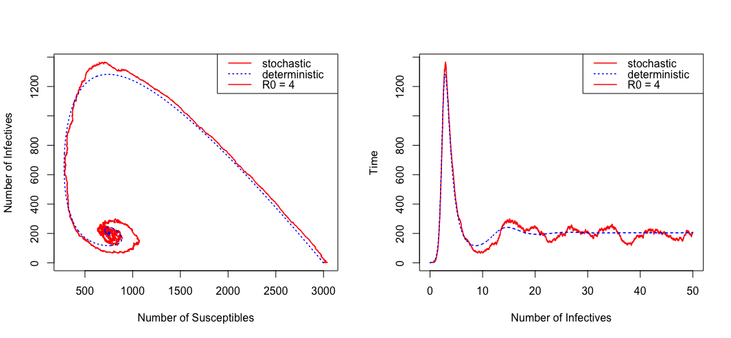
Figure 4: SIR epidemic with parameter $(R_{0},\mu,\gamma)=(4,0.1,1)$

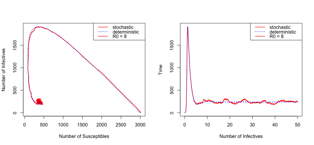
Figure 5: SIR epidemic with parameter $(R_{0},\mu,\gamma)=(8,0.1,1)$

2.2 The Stichastic Model of SIR with Demography

Suppose that $p_{sir}(t)=P\{S(t)=s,I(t)=i,R(t)=r\}$. Using the transition rates in Table 1, we can construct forward Kolmogorov equation as follows

$$p_{sir}^{\prime}(t) =p_{s-1,i,r}(t)\cdot(\mu n)+p_{s+1,i,r}(t)\cdot(\mu(s+1))+p_{s,i+1,r}(t)\cdot$$

$$\quad(\mu(i+1))+p_{s,i,r+1}(t)\cdot(\mu(r+1))+p_{s+1,i-1,r}(t)\cdot$$

$$\quad\left(\frac{\lambda}{n}(s+1)(i-1)\right)+p_{s,i+1,r-1}(t)\cdot(\gamma(i+1))-p_{sir}(t)\cdot$$

$$\quad\left(\mu(n+s+i+r)+\frac{\lambda}{n}si+\gamma i\right).$$ (3)

Now, consider Figures 3, 4, and 5. The SIR process certainly has similar behaviour to SIS. In Figure 3, we can see a certain deviance between the deterministic and the stochastic models, but in Figures 4 and 5 the stochastic model seems to settle down in equilibrium faster than in Figure 3 and the deterministic model also approximates nicely. This equilibrium is reached at point $\left(R_{0}^{-1},\frac{\displaystyle\mu}{\displaystyle\mu+\gamma}-\frac{\displaystyle\mu}{\displaystyle\lambda}\right)$. By changing $\mu$, we can see that the threshold theorem is still applied but the equilibrium point is shifted.

Another interesting fact about SIR epidemic modelling with demography is how the dynamic of susceptible size in the absence of infective. Recall equation (1a). In the absence of infective, the proportion of susceptibles in the population is

$$\frac{dx(t)}{dt}=\mu(1-x(t))$$

with solution $x(t)=1-\displaystyle\frac{m}{n}e^{-\mu t}$, given the initial value $x(0)=1-\frac{\displaystyle m}{\displaystyle n}\approx 1$.

We know that when $R_{0}>1$, there is possibility that the epidemic will die out very quickly. Suppose that the epidemic survives and $m=1$. Then, in the early stage of epidemic, we can approximate the process of infection using the birth– death process with birth rate $\lambda x(t)$ and death rate $(\gamma+\mu)$. Suppose that $p_{i}(t)$ denotes the probability $Y_{n}(t)=i$. Then, the modified forward Kolmogorov equation in (3) becomes

$$p_{i}^{\prime}(t)=(i+1)(\gamma+\mu)p_{i+1}(t)+(i-1)\lambda(t)p_{i-1}(t)-i(\lambda(t)+\gamma+\mu)p_{i}(t).$$ (4)

From the equation (3), the time to extinction of the SIR epidemic must satisfy the differential equation

$$p_{\cdot 0\cdot}^{\prime}(t) =p_{\cdot 1\cdot}(t)\cdot\mu+p_{\cdot 1\cdot}(t)\cdot\gamma$$

$$=(\mu+\gamma)p_{\cdot 1\cdot}(t)$$ (5)

The solution of eq. (4) can be seen in Kendall [11] Now consider Figure 6. When we set $R_{0}>1$, there are essentially two behaviours we should notice. First, given the small proportion of initial infectious individuals the infection may die out very quickly as in Figure 6. Second, if it survives, then it will enter endemic level at some $t$ as we can see in Figures 3, 4, and 5, where the osilation around the deterministic model becomes damped and the process is now mimicking the deterministic version.

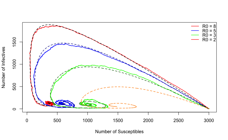
(a) Parameter $\mu=0.05$

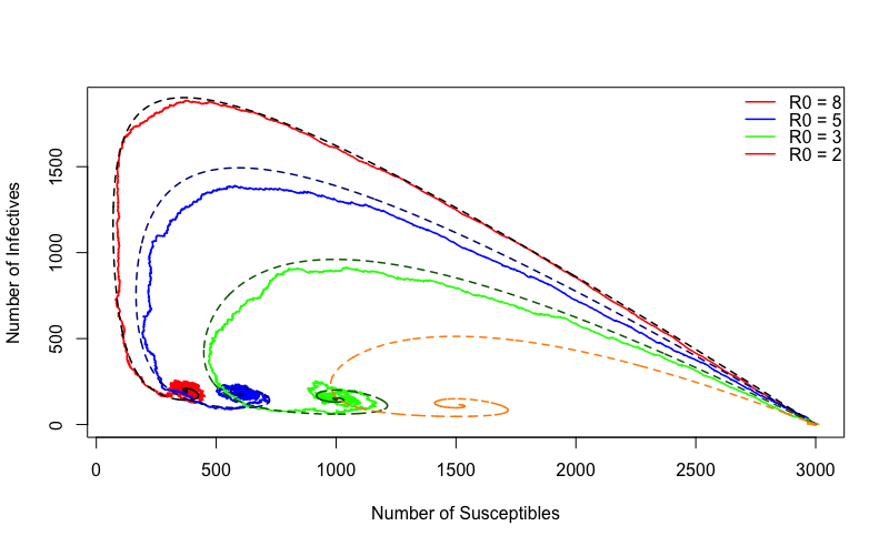
(b) Parameter $\mu=0.08$

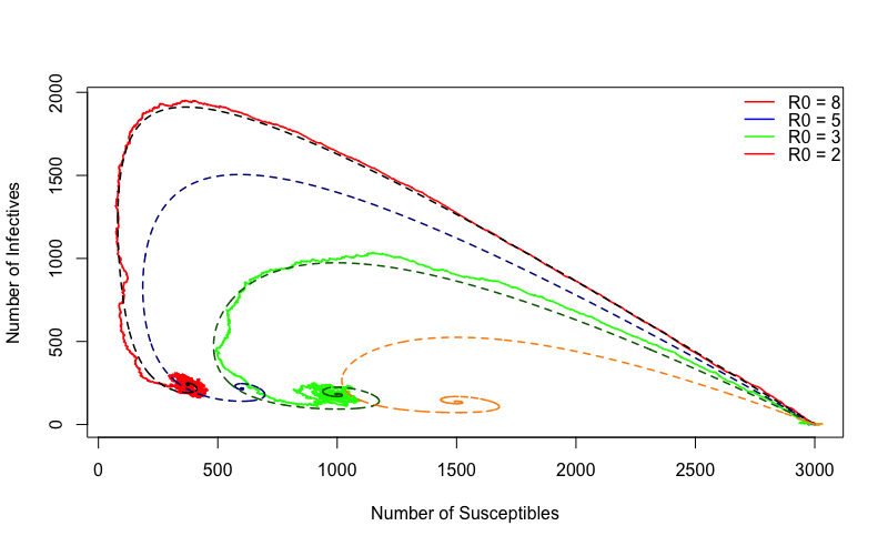
(c) Parameter $\mu=0.1$

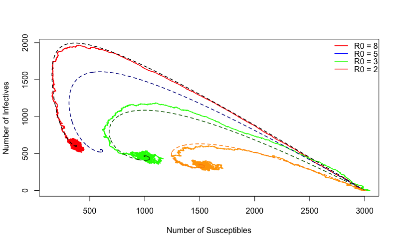
(d) Parameter $\mu=0.3$

Figure 6: SIR with demography with $(n,m,\gamma)=(3000,1,1)$

2.3 The Probability of Extinction when $R_{0}>1$

The second behaviour can be explained according to the density dependent process and using law of large number [14]. Now, we need to show that there is non–zero probability that the process will die out even though $R_{0}>1$.

First, we begin with defining $p_{i}(t)$ in more detail. The forward Kolmogirov equation is given in eq. (4) where $p_{1}(0)=1$ and $p_{i}(t)=0$ for $i<0$. The pgf of $p_{i}(t)$ is

$$\varphi(z,t)=\sum_{k=0}^{\infty}p_{k}(t)z^{k}$$ (6)

and it must satisfy

$$\frac{\displaystyle\partial\varphi}{\displaystyle\partial t}=(z-1)(\lambda(t)z-(\gamma+\mu))\frac{\displaystyle\partial\varphi}{\displaystyle\partial z}$$ (7)

with boundary condition $\varphi(z,0)=z$.

We use the result of Kendall [11] that the solution of eq. (4) is

$$p_{i}(t)=(1-p_{0}(t))\cdot(1-\eta_{t})\eta_{t}^{i-1}\quad\text{for all }i\geq 1$$ (8)

where $\eta_{t}$ is a function of $t$. Suppose we denote $p_{0}(t)=\xi$ and $\eta_{t}=\eta\neq 1$, then

$$\varphi(z,t) =\xi+\sum_{k=1}^{\infty}p_{k}(t)z^{k}$$

$$=\xi+(1-\xi)(1-\eta)\sum_{k=1}\eta^{k-1}z^{k}$$

$$=\frac{\xi+(1-\xi-\eta)z}{1-\eta z}.$$ (9)

Now, by differentiating equation (9) with respect to $t$ and $z$ and then substituting to equation (7), yields

$$(\eta\xi^{\prime}-\eta^{\prime}\xi)+\eta^{\prime}=\lambda(t)(1-\eta)(1-\xi)$$ (10)

and recall that $p_{0}^{\prime}(t)=\xi^{\prime}=(\gamma+\mu)p_{1}(t)$ and using the result from Kendall……… $p_{1}(t)=(1-\xi)(1-\eta)$. Thus,

$$\xi^{\prime}=(\gamma+\mu)(1-\xi)(1-\eta)$$ (11)

Therefore, by letting $U=1-\xi$ and $V=1-\eta$, eq. (10) and (11) become

$$-U^{\prime} =(\gamma+\mu)UV$$

$$\frac{U^{\prime}}{U} =-(\gamma+\mu)V$$ (12a)

$$-(1-V)U^{\prime}+V^{\prime}(1-U)-V^{\prime} =\lambda(t)VU$$

$$-(1-V)\frac{U^{\prime}}{U}-V^{\prime} =\lambda(t)V\$$

$$(\gamma+\mu)(1-V)V-V^{\prime} =\lambda(t)V$$

$$(\gamma+\mu-\lambda(t))V-(\gamma+\mu)V^{2} =V^{\prime}.$$ (12b)

Letting $W=\frac{\displaystyle 1}{\displaystyle V}$ implies that $W^{\prime}=-\frac{\displaystyle V^{\prime}}{\displaystyle V^{2}}=-W^{2}V^{\prime}$, then equation (12b) becomes

$$W^{\prime}+(\gamma+\mu-\lambda(t))W =(\gamma+\mu).$$ (13)

Note that equation (13) is the first order differential equation with general solution

$$W=\frac{(\gamma+\mu)\displaystyle\int_{0}^{t}e^{\rho(u)}du+c}{e^{\rho(t)}}$$ (14)

where $\rho(t)=\displaystyle\int_{0}^{t}\gamma+\mu-\lambda(u)du$. Now, recall that $p_{1}(0)=1$. It implies that $\xi_{0}=p_{0}(0)=0=p_{i}(0)=\eta_{0}$ for all $i\neq 1$. Consequently, $U_{0}=1-\xi_{0}=1=V_{0}=1-\eta_{0}$ and $W_{0}=\frac{\displaystyle 1}{\displaystyle V_{0}}=1$. Therefore, using initial condition at $t=0$ yields

$$W=e^{-\rho(t)}\left(1+(\gamma+\mu)\int_{0}^{t}e^{\rho(u)}du\right).$$ (15)

Returning to equation (12a) and (12b). Since $V=\frac{\displaystyle 1}{\displaystyle W}$, then it yields $\eta=1-V=1-\frac{\displaystyle 1}{\displaystyle W}$ and $\xi=1-U=1-\frac{\displaystyle e^{-\rho(t)}}{\displaystyle W}$. Note that $p_{0}(t)=\eta$. So,

$$p_{0}(t) =1-\frac{e^{-\rho(t)}}{e^{-\rho(t)}\left(1+(\gamma+\mu)\displaystyle\int_{0}^{t}e^{\rho(u)}du\right)}$$

$$=1-\frac{1}{\left(1+(\gamma+\mu)\displaystyle\int_{0}^{t}e^{\rho(u)}du\right)}$$

where $\rho(t)=\displaystyle\int_{0}^{t}(\gamma+\mu)-\lambda(u)du$.

Note that if we let $R_{0}=\frac{\displaystyle\lambda(t)}{\displaystyle\gamma+\mu}>1$, then equation (LABEL:eq:sir.final.prob.ext) lays in $(0,1)$. This explains mathematically the extinction in Figure 6 and also supports the branching process theory. Otherwise, by letting $R_{0}\leq 1$, and if we let $t\rightarrow\infty$, then $\left(1+(\gamma+\mu)\displaystyle\int_{0}^{t}e^{\rho(t)}du\right)\rightarrow\infty$. Consequently, $p_{0}(t)\rightarrow 1$ as $t\rightarrow\infty$. This result is not surprising since we have already known that when $R_{0}\leq 1$, the stable stage of the epidemic process is attained in the disease-free stage.

3 Conclusion

According to the threshold theorem, epidemic can only occur if the initial number of susceptibles is larger than some critical value, which depends on the parameters under consideration (Ball, 1983). Usually, it is expressed in terms of epidemic reproductive ratio number, $R_{0}$. This quantity is defined as the expected number of contacts made by a typical infective to susceptibles in the population.

We have successfully showed that both deterministic and stochastic models performed similar results when $R_{0}\leq 1$. That is, the disease-free stage in the epidemic. But when $R_{0}>1$, the deterministic and stochastic approaches had different interpretations. In the deterministic models, both the SIS and SIR models showed an outbreak of the disease and after some time $t$, the disease persisted and reached endemic-equilibrium stage. The stochastic models, on the other hands, had different interpretations. If we let the population size be sufficiently large, the epidemic might die out or survive. There were essentially two stages to this model. First, the infection might die out in the first cycle. If it did, then it would happen very quickly, just like the branching process theory described. Second, if it survived the first cycle, the outbreak was likely to occur, but after some time $t$, it would reach equilibrium just like the deterministic version. In fact, the stochastic models would mimic the deterministic’s paths and be scattered randomly around their equilibrium point.

4 References

References

- [1] H. Andersson and B. Djehiche, “A Threshold Limit Theorem for the Stochastic Logistic Epidemic”, J. Appl. Prob. 35, 662–670 (1998).
- [2] N. T. Bailey, The Mathematical Theory of Infectious Diseases and its Applications, 2nd edition (Griffin, London, 1975).
- [3] F. G. Ball, “The Threshold Behaviour of Epidemic Models”, J. Appl. Prob. 20, 227–241 (1983).
- [4] F. G. Ball, Epidemic Thresholds. Encyclopedia of Biostatistics. 3. (John Wiley & Sons, Chichester, 1998).
- [5] F. G. Ball and O. D. Lyne, “Optimal Vaccination Policies for Stochastic Epidemics among a Population of Households”, Submitted Math. Bioscie. 177–178, 333–354 (2002).
- [6] P. G. Ballard, N. G. Bean, J. V. Ross, “The Probability of Epidemic Fade-Out is Non-Monotonic in Transmission Rate for Markovian SIR Model with Demography”, Submitted J. Theoretical Bio. 393, 170–178 (2016).
- [7] H. Andersson and T. Britton, Stochastic Epidemic Models and Their Statistical Analysis (Springer, New York, 2000).
- [8] S. N. Ethier and T. G. Kurtz, Markov Processes Characterization and Convergence (Wiley, New York, 1982).
- [9] s.‘Karlin, A First Course in Stochastic Processes. 2nd ed. (Academic Press Inc., California, 1975).
- [10] F. P. Kelly, Reversibility and Stochastic Networks (Cambridge University Press, Cambridge, 2011).
- [11] D. G. Kendall, “On the Generalized Birth and Death Process”, The Annals of Mathematical Statistics 19, 1–15 (1948).
- [12] I. Nåsell, “Stochastic Models of Some Endemic Infections”, Math. Bioscie. 179, 1–19 (2002).
- [13] S.M. Ross, Introduction to Probability Models. 9th ed. (Elsevier Inc., London, 2007).
- [14] K. Susvitasari, “The Stochastic Modelling on SIS Epidemic Modelling”, Journal of Physics: Conference Series 795 (2017).