A numerical method to solve a phaseless coefficient inverse problem from a single measurement of experimental data.

Abstract

We propose in this paper a globally numerical method to solve a phaseless coefficient inverse problem: how to reconstruct the spatially distributed refractive index of scatterers from the intensity (modulus square) of the full complex valued wave field at an array of light detectors located on a measurement board. The propagation of the wave field is governed by the 3D Helmholtz equation. Our method consists of two stages. On the first stage, we use asymptotic analysis to obtain an upper estimate for the modulus of the scattered wave field. This estimate allows us to approximately reconstruct the wave field at the measurement board using an inversion formula. This reduces the phaseless inverse scattering problem to the phased one. At the second stage, we apply a recently developed globally convergent numerical method to reconstruct the desired refractive index from the total wave obtained at the first stage. Unlike the optimization approach, the two-stage method described above is global in the sense that it does not require a good initial guess of the true solution. We test our numerical method on both computationally simulated and experimental data. Although experimental data are noisy, our method produces quite accurate numerical results.

Key words: phaseless coefficient inverse problem, phased coefficient inverse problem, optical experimental data, single measurement, new numerical method, numerical reconstructions

AMS subject classification: 35R30, 78A46, 65C20

1 Introduction

Using the apparatus of the Riemannian geometry and asymptotic analysis, we construct in this paper a new numerical method for the solution of a 3D Phaseless Coefficient Inverse Problem (phaseless CIP) for the Helmholtz equation with the data resulting from a single measurement event. The unknown coefficient of the Helmholtz equation is $n^{2}\left(\mathbf{x}\right),\mathbf{x}\in\mathbb{R}^{3},$ where $n\left(\mathbf{x}\right)\geq 1$ is the spatially distributed refractive index. Our method computes locations and refractive indices of unknown scatterers using experimentally measured intensity (i.e. the square modulus) of the complex valued wave field. That wave field is the solution of the Helmholtz equation. The phase was not measured. We verify the accuracy of our computations via applying the same numerical method to computationally simulated data.

Measurements were conducted on a part of a plane outside of scatterers. Only a single direction of the incident plane wave on many wavelengths was used, which means a single measurement event. This is more difficult than the case of multiple measurements. The experimental data were collected by ourselves. The authors are unaware about other publications in which a 3D phaseless CIP would be computationally solved for the case when the experimental intensity data would be collected on several wavelengths and for a single measurement event.

Our scatterers are microspheres of the diameter of 6 $\mu m$ (micron). Our experimental data were collected for the case of the vertically propagated white light. To obtain data on an interval of frequencies, the light was filtered on six (6) wavelengths ranging from 0.420$\mu m$ to 0.671$\mu m.$ Following, e.g., [63], to measure the light intensity, we have used the detector array which is available in the camera of the Samsung Galaxy S3 mobile telephone unit. The idea of [63] is to built an extremely low weight optical system.

We used white light source with a set of narrow band filters to provide various illumination wavelengths because this technique can be used in combination with standard microscopes and in any environment such for example as clinical environment. This way we have measured the intensity of only the full wave field. However, since the case of the full wave field was not considered in the above cited publications on phaseless CIPs, we develop here a significantly new numerical method for our phaseless CIP. Phaseless CIPs for the case when the intensity of the full wave field is measured were also studied analytically in [61] for both Helmholtz and Schrödinger equations. In this case the medium is simultaneously illuminated by two point sources and many such pairs of sources are used. This does not work, however, for our experimental arrangement, since we have only a single direction of the incident plane wave.

First, we establish an inversion formula to approximate the wave field at the measurement site. This is considered as the first stage of our numerical method. This inversion formula is very interesting because the reconstruction of the complex number $z=|z|e^{{\mathrm{i}}\arg z}$ from $z$ is not unique. In this paper, we can successfully derive this approximate reconstruction by using an asymptotic behavior of the wave field and proving a priori bound for the scattering wave. After this stage, we obtain a Phased Coefficient Inverse Problem (phased CIP). On the second stage, we solve that phased CIP to reconstruct the unknown coefficient of the Helmholtz equation. It is on the second stage when we reconstruct locations and refractive indices of those microspheres. The numerical solution of the phased CIP is found using the globally convergent numerical method, which was recently developed in [38], also, see [46, 54, 53] for the performance of this method on microwave experimental backscattering data

Our interest in phaseless CIPs is motivated by applications to optical imaging of such small objects as, e.g. biological cells and microspheres. Sizes of biological cells are usually in the interval of $\left(5,100\right)\mu m$ [57]. To optically image such small targets, one should use light sources, in which case the wavelengths are of $1\mu m$ range. The wavelength $\lambda=1\mu m$ corresponds to the frequency $\omega\approx 300,000$ Gigahertz. It is currently impossible, however, to arrange stable measurements of the phase for such high frequencies. Only the intensity of the scattered wave field can be reliably measured on these frequencies [56, 62].

While we have measured the intensity of the full wave field, it is also possible sometimes to measure the intensity of the scattered wave field. On the other hand, a number of past works for phaseless CIPs of the first author with coauthors were devoted to the analytical reconstruction procedures for the case when the intensity of the scattered wave field is measured [40, 41, 42, 43, 37]. To arrange experimental measurements for this case, one needs to work with tunable lasers, which would operate on several wavelengths.

The question on how to solve the inverse scattering problem without the phase information was probably first posed in the book of Chadan and Sabatier [15, Chapter 10] published in 1977. Fifteen years later, the first uniqueness result for this problem in the 1D case was established in [45], also see [1] for a follow up result. Next, the first uniqueness result in 3D was obtained in [32]. Since then, the 3D phaseless CIPs were studied intensively. In [39] a modified reconstruction procedure of [42] was numerically implemented. Multiple locations of the point source at multiple frequencies were used in [42, 39]. Unlike this, in [37] the case of a single direction of the incident plane wave on a frequency interval was numerically implemented. We refer the reader to other versions of the uniqueness theorems for 3D phaseless CIPs in [31, 33, 34, 44]. As mentioned above, the analytic reconstruction procedures in for 3D phaseless CIPs were proposed in [40, 41, 42, 43] for the  case when the intensity of the scattered rather than full wave field is measured.

We now refer to other approaches to phaseless inverse scattering problems. In [7, 8] a phaseless CIP for Helmholtz equation was solved numerically using Kirchhoff migration and Born approximation. While coefficients of partial differential equations are subjects of interests in all above cited works, there is also a significant interest in the reconstruction of surfaces of scatterers from the phaseless data. In this regard we refer to publications [2, 5, 6, 25, 23, 24, 50] and references cited therein. We also mention the problem of the reconstruction of a compactly supported function from the absolute value of its Fourier transform [29, 35] as well as a closely related problem of the solution of the autoconvolution equation [18, 14, 13].

As to the phased CIPs, they arise in many real world applications including detection and identification of explosives, non-destructive testing, medical imaging, and geophysics prospecting. In general, CIPs are nonlinear and ill-posed. The developments of the numerical methods for CIPs are challenging. Due to a large variety of applications, there is a huge literature on numerical reconstruction methods for these problems.  We refer here to a few publications and references cited therein [3, 4, 2, 10, 16, 17, 19, 20, 47, 22, 50, 49, 51].

We call a numerical method for a CIP globally convergent if there is a theorem, which claims that this method delivers at least one point in a sufficiently small neighborhood of the exact solution without any advanced knowledge of this neighborhood. As to the numerical method of [38], which is used here, Theorem 6.1 of [38] ensures its global convergence. While the above mentioned globally convergent numerical method works for CIPs with single measurement data, we also refer to [28, 26, 27] for a global reconstruction technique for a CIP with the data resulting from multiple measurements. The idea of these references is based on an extension to the 2D case of the well-known Gelfand-Krein-Levitan method, which works for a 1D CIP.

In Section 2, we state our phaseless CIP. In Section 3, we recall the asymptotic behavior of the solution of the Helmholtz equation when the wave number tends to infinity. In Section 4 we estimate both analytically and numerically the intensity of the scattered wave field and, using this estimate derive inversion formulae which enable us to approximate the wave field at the measurement site. In Section 5, we briefly outline the globally convergent numerical method of [38]. In Section 6, we describe the procedure of the collection of the experimental data. In Section 7 we present our numerical results. In Section 8 We summarize results of this paper in Section 8.

2 Problem statement

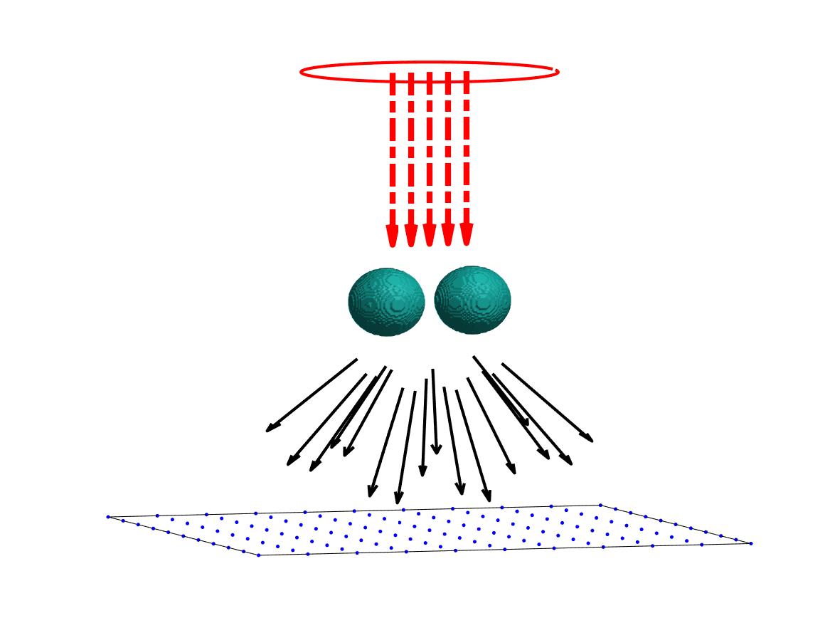
Figure 1: A schematic diagram of measurements.

In this section we formulate the phaseless CIP of this paper. To this end we first briefly describe the direct scattering problem. Suppose that an object is illuminated by an incident plane wave. The interaction of this incident wave with the object produces the scattered wave, see Figure 1. The total wave field is the sum of the incident wave and the scattered wave.

We denote $\mathbf{x}=\left(x_{1},x_{2},x_{3}\right)$ points of $\mathbb{R}^{3}$. Let $\Omega\subset\mathbb{R}^{3}$ be a bounded domain with a piecewise smooth boundary $\partial\Omega$, containing the scatterers. It is convenient for our computational purpose to specify the domain $\Omega$ as

$$\Omega=\left\{\mathbf{x}:\left|x_{1}\right|,\left|x_{2}\right|<b,x_{3}\in\left(-d_{1},d_{2}\right)\right\},$$ (2.1)

where $b,d_{1},d_{2}>0$. We also denote $\Gamma$ one of sides of $\Omega,$

$$\Gamma=\left\{\mathbf{x}:\left|x_{1}\right|,\left|x_{2}\right|<b,x_{3}=d_{2}\right\}\subset\partial\Omega.$$ (2.2)

Let the function $n\left(\mathbf{x}\right)$, defined for all $\mathbf{x}\in\mathbb{R}^{3},$ represent the spatially distributed refractive index of the medium. We assume that microspheres of our interest are located in the domain $\Omega.$ Assume that

$$n(\mathbf{x})=1\mbox{ for all }\mathbf{x}\in\mathbb{R}^{3}\setminus\overline{\Omega}\quad\mbox{ and }\quad n(\mathbf{x})\geq 1\mbox{ for all }\mathbf{x}\in\mathbb{R}^{3}.$$ (2.3)

Condition (2.3) means that the dielectric constant of the background is scaled to be 1 and that of the scattering object is greater than 1. Let $k>0$ be the wave number, consider the incident plane wave

$$u_{\mathrm{i}nc}(\mathbf{x},k)=e^{\mathrm{i}kx_{3}}.$$ (2.4)

Denote by $u_{\mathrm{sc}}(\mathbf{x},k)$ the scattering wave. Then, the total wave field

$$u(\mathbf{x},k)=u_{\mathrm{i}nc}(\mathbf{x},k)+u_{\mathrm{sc}}(\mathbf{x},k)$$ (2.5)

is governed by the Helmholtz equation with the Sommerfeld outgoing radiation condition at the infinity,

$$\left\{\begin{array}[]{rcll}\Delta u(\mathbf{x},k)+k^{2}n^{2}(\mathbf{x})u(\mathbf{x},k)&=&0&\mathbf{x}\in\mathbb{R}^{3},\\ \partial_{|\mathbf{x}|}u_{\mathrm{sc}}(\mathbf{x},k)-\mathrm{i}ku_{\mathrm{sc}}(\mathbf{x},k)&=&o(|\mathbf{x}|^{-1})&|\mathbf{x}|\rightarrow\infty.\end{array}\right.$$ (2.6)

Let the number

$$R>d_{2}.$$ (2.7)

Define the plane $P$ and a square $P_{\text{meas}}\subset P$ as

$$P=\{\mathbf{x=}(x_{1},x_{2},R):x_{1},x_{2}\in\mathbb{R}\},\quad P_{\text{meas}}=\{\mathbf{x=}(x_{1},x_{2},R):\left|x_{1}\right|,\left|x_{2}\right|<b\}.$$ (2.8)

We call $P$ the “measurement plane.” Measurements of the intensity are conducted on the square $P_{\text{meas}}$ for the wave numbers $k\in[\underline{k},\overline{k}].$ Here, the interval $k\in[\underline{k},\overline{k}]$ represents the allowable range of wave numbers.

Problem 2.1 (The phaseless coefficient inverse scattering problem).

Let $1\ll\underline{k}<\overline{k}<\infty$. Assume that the function $f(\mathbf{x},k),$

$$f(\mathbf{x},k)=|u(\mathbf{x},k)|^{2},\quad\mathbf{x}\in P_{\text{meas}},k\in[\underline{k},\overline{k}]$$ (2.9)

is known. Determine the function $n(\mathbf{x})$ for $\mathbf{x}\in\Omega$.

Remark 2.1 (A comment on the Helmholtz equation).

Although the full Maxwell’s system is the right model to describe the propagation of the total wave field, we use the Helmholtz equation (2.6) in this paper. We have numerically verified in [37, Section 8] that if the incident wave field has the form $(0,u_{inc}(\mathbf{x},k),0)$, then $E_{2}(\mathbf{x},k)$, the second component of the electric wave field satisfying the Maxwell’s system, matches well the total wave field $u(\mathbf{x},k)$. The study for the phaseless coefficient inverse problem for Maxwell’s system with general incident wave field is considered as future research.

It is well-known that the Helmholtz equation (2.6) can be reformulated as the Lippmann-Schwinger equation (see [17, Chapter 8])

$$u(\mathbf{x},k)=e^{\text{i}kx_{3}}+k^{2}\displaystyle\int\limits_{\Omega}\frac{\exp(\mathrm{i}k|\mathbf{x}-\mathbf{\xi}|)}{4\pi|\mathbf{x}-\mathbf{\xi}|}(n^{2}(\mathbf{\xi})-1)u(\mathbf{\xi},k)d\mathbf{\xi,}\quad\mathbf{x}\in\mathbb{R}^{3}.$$ (2.10)

Using the method in [48, 52], we solve numerically the integral equation (2.10) to computationally simulate the data for the phaseless CIP. In addition, we solve this equation iteratively on the second stage of our reconstruction procedure.

3 Asymptotic behavior of the total wave as $k\rightarrow\infty$

In this section we establish the asymptotic behavior of the function $u\left(\mathbf{x},k\right)$ and at $k\rightarrow\infty.$ Although results of this section follow from [43], we need to formulate these results again here since we essentially use them in our numerical method.

3.1 Geodesic lines

In addition to conditions (2.3) imposed on the function $n\left(\mathbf{x}\right),$ we also assume that

$$n\in C^{15}\left(\mathbb{R}^{3}\right).$$ (3.1)

The smoothness condition (3.1) is a technical one. It was used in [43] to prove an analog of Theorem 3.1. And that analog, in turn was derived in [43] using the construction of the solution of the Cauchy problem for a certain hyperbolic equation in [59]. This construction technically needs (3.1). In addition, usually extra smoothness assumptions are not of a great concern in the theory of CIPs, see, e.g. Theorem 4.1 in [58].

The Riemannian metric generated by the function $n\left(\mathbf{x}\right)$ is

$$d\tau(\mathbf{x})=n(\mathbf{x})|d\mathbf{x}|,\quad|d\mathbf{x}|=\sqrt{(dx_{1})^{2}+(dx_{2})^{2}+(dx_{3})^{2}}.$$ (3.2)

Let the number $a>d_{1}.$ Consider the plane

$$P_{a}=\{\mathbf{x}=(x_{1},x_{2},-a):x_{1},x_{2}\in\mathbb{R}\}.$$

Then by (2.1) and (2.7), both $\Omega$ and $P$ are contained in $\left\{x_{3}>-a\right\}.$ We assume below without further mentioning the condition about the regularity of geodesic lines:

Assumption (Regularity of geodesic lines).

For any point $\mathbf{x}\in\mathbb{R}^{3}$ there exists a unique geodesic line $\Gamma(\mathbf{x},a)$, with respect to the metric $d\tau$ in (3.2) connecting $\mathbf{x}$ with the plane $P_{a}$ and perpendicular to $P_{a}$.

Again, we need this assumption only for Theorem 3.5. But we do not verify it in our numerical studies. A sufficient condition of the regularity of geodesic lines is (see [60])

$$\sum\limits_{i,j=1}^{3}\frac{\partial^{2}\ln\left(n(\mathbf{x})\right)}{\partial x_{i}\partial x_{j}}\xi_{i}\xi_{j}\geq 0,\quad\text{for all }\mathbf{x}\in\overline{\Omega},\mathbf{\xi}\in\mathbb{R}^{3}.$$

For an arbitrary point $\mathbf{x}\in\left\{x_{3}>-a\right\}$ the travel time along the geodesic line $\Gamma(\mathbf{x},a)$ from the plane $P_{a}$ to the point $\mathbf{x}$ is (see [43])

$$\tau(\mathbf{x})=\displaystyle\int\limits_{\Gamma(\mathbf{x},a)}n\left(\mathbf{\xi}\right)d\sigma.$$ (3.3)

The following theorem follows immediately from formulae (4.24)-(4.26) of [43]:

Theorem 3.1.

Let $G\subset\left\{x_{3}>-a\right\}$ be an arbitrary bounded domain such that $\Omega,P_{\text{meas}}\subset G.$ Then the following asymptotic behavior of the solution of the problem (2.5), (2.6) holds

$$u(\mathbf{x},k)=A(\mathbf{x})\exp(\mathrm{i}k\tau(\mathbf{x}))\left(1+g(\mathbf{x},k)\right),\quad\mathbf{x}\in G,k\rightarrow\infty,$$ (3.4)

where functions $A(\mathbf{x})>0$ and $g(\mathbf{x},k)$ are smooth and also for $j=1,2,3$

$$g(\mathbf{x},k),\partial_{k}^{j}g(\mathbf{x},k)=O\left(1/k\right),\quad\mathbf{x}\in G,k\rightarrow\infty.$$ (3.5)

Corollary 3.1 follows immediately from (3.4), (3.5):

Corollary 3.1.

We have

$$A(\mathbf{x})=\lim_{k\rightarrow\infty}|u(\mathbf{x},k)|,\text{ }\forall\mathbf{x}\in G.$$ (3.6)

Using (3.4), we obtain the following approximate formula for the scattered wave field $u_{\text{sc}}\left(\mathbf{x},k\right)$ for sufficiently large values of the wave number $k$:

$$u_{\text{sc}}\left(\mathbf{x},k\right)=A\left(\mathbf{x}\right)\exp\left(\text{i}k\tau\left(\mathbf{x}\right)\right)-e^{\text{i}kx_{3}},\text{ }\mathbf{x}\in G.$$ (3.7)

4 An analytical upper estimate of $\left|u_{\text{sc}}\left(\mathbf{x},k\right)\right|^{2}$ and an approximate inversion formula

To derive our approximate inversion formula, we need to assume that the function $\left|u_{\text{sc}}\left(\mathbf{x},k\right)\right|^{2}$ is sufficiently small. We have computationally estimated $\left|u_{\text{sc}}\left(\mathbf{x},k\right)\right|^{2}$ for those parameters which we use in our studies of both computationally simulated and experimental data. Indeed, let $k$ be the dimensionless wave number, see Section 6 for details. We have measured data for $k\in\left[93.59,149.52\right],$ which corresponds to the wavelengths $\lambda\in\left[0.420,0.671\right]\mu m$. However, we have observed that data are too noisy for $k\notin\left[108.3,119.6\right],$ see (6.3). Hence, we set

$$k\in\left[\underline{k},\overline{k}\right]=\left[108.3,119.6\right].$$ (4.1)

We have computationally simulated the data for the interval of wave numbers (4.1) via the numerical solution of equation (2.10). In doing so, we have modeled the microspheres by exactly the same parameters as they are in the experiment. Figures 2a–2b display the graph of the function

$$\varphi(k)=\max_{{\mathbf{x}}\in P_{\mathrm{m}eas}}|u_{\mathrm{s}c}({\mathbf{x}},k)|^{2}\quad k\in[\underline{k},\overline{k}].$$ (4.2)

These illustrations indicate that our assumption about the smallness of the function $\varphi(k)$ is might be true, at least for models and the range of the parameters used in this paper.

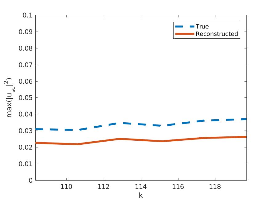
(a) Case of one microsphere described in Section 7.1. In this case $\varphi\left(k\right)\leq 0.038.$

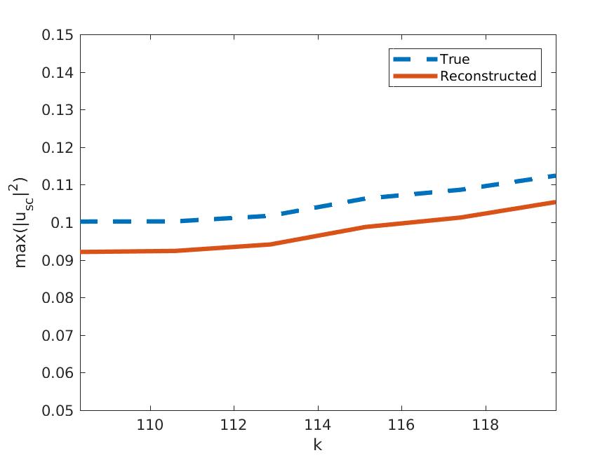
(b) The case of two microspheres described in Section 7.2. In this case $\varphi\left(k\right)\leq 0.115.$

Figure 2: The function $\varphi\left(k\right)$ defined in (4.2) is displayed for $k\in\left[\underline{k},\overline{k}\right]=\left[108.2,119.6\right].$ It is computed from the simulated data generated from exactly the same models and parameters as in the experiments. The function $\varphi\left(k\right)$ is sufficiently small. Here, “true” means the function $\varphi\left(k\right)$ results from the solution of equation (2.10). “Reconstructed” means that the function is computed from the reconstruction of the total wave $u({\mathbf{x}},k)$ using the method using formula (4.21) in this section and (2.5) .

4.1 An analytical upper estimate

It is desirable to provide an analytical justification to our computational finding (Figure 2) an upper bound for the function $\varphi(k),$ $k\in\left[\underline{k},\overline{k}\right].$ It follows immediately from (2.4), (2.5) and (2.10) that

$$u_{\text{sc}}(\mathbf{x},k)=k^{2}\displaystyle\int\limits_{\Omega}\frac{\exp(\mathrm{i}k|\mathbf{x}-\mathbf{\xi}|)}{4\pi|\mathbf{x}-\mathbf{\xi}|}\left(n^{2}(\mathbf{\xi})-1\right)u(\mathbf{\xi},k)d\mathbf{\xi,}\text{ }\mathbf{x}\in P_{\text{meas}}.$$ (4.3)

We can see from (4.3) that $|u_{\mathrm{s}c}({\mathbf{x}},k)|$ grows at the order $O(k^{2})$ as $k\to\infty$. Our goal in Theorem 4.6 is to decrease that growth to be $O(k)$. Since by (2.8), $\mathbf{x=}\left(x_{1},x_{2},R\right)$ on $P_{\text{meas}}.$ Assuming that $R\gg\max\left(b,1\right)$ and using the well-known formula for the far field approximation, we obtain from (4.3)

$$u_{\text{sc}}(\mathbf{x},k)=\frac{k^{2}}{4\pi R}e^{\text{i}kR}\displaystyle\int\limits_{\Omega}e^{-\text{i}k\xi_{3}}\left(n^{2}(\mathbf{\xi})-1\right)u(\mathbf{\xi},k)d\mathbf{\xi,}\quad\mathbf{x}\in P_{\text{meas}}.$$ (4.4)

We use in (4.4) “$=$” instead of “$\approx$” only for the convenience of the a priori bound established in Theorem 4.6 below.

Theorem 4.1.

Assume that

$$\left|\tau_{\xi_{3}}\left(\mathbf{\xi}\right)-1\right|\geq\beta=const.>0,\quad\forall\mathbf{\xi}\in\Omega.$$ (4.5)

Then the following estimate is valid for the function $u_{\text{sc}}(\mathbf{x},k)$ given in (4.4)

$$\left|u_{\text{sc}}(\mathbf{x},k)\right|\leq C\frac{k}{4\pi R}\left(1+O\left(1/k\right)\right),\quad\text{ }\mathbf{x}\in P_{\text{meas}},k\rightarrow\infty,$$ (4.6)

where the number $C>0$ depends only on the domain $\Omega,$ functions $A\left(\mathbf{\xi}\right),c\left(\mathbf{\xi}\right)$ for $\mathbf{\xi}\in\Omega$ and the number $\beta$ in (4.5).

Proof. Since the function $n^{2}(\mathbf{x})-1=0$ outside of the domain $\Omega$, then by (2.1), we can assume that $n^{2}(\mathbf{x})-1=0$ for $\left|\mathbf{x}\right|>r,$ where the number $r>0$ is such that $B\left(r\right)=\left\{\left|\mathbf{x}\right|<r\right\}\subset\Omega.$ Using $u(\mathbf{\xi},k)=A\left(\mathbf{\xi}\right)e^{\text{i}k\tau\left({\mathbf{\xi}}\right)}\left(1+O\left(1/k\right)\right)$ and substituting in (4.4), we obtain

$$u_{\text{sc}}(\mathbf{x},k)=\frac{k^{2}}{4\pi R}e^{\text{i}kR}\displaystyle\int\limits_{\xi_{1}^{2}+\xi_{2}^{2}<r^{2}}d\xi_{1}d\xi_{2}\displaystyle\int\limits_{-\sqrt{r^{2}-\xi_{1}^{2}-\xi_{2}^{2}}}^{\sqrt{r^{2}-\xi_{1}^{2}-\xi_{2}^{2}}}e^{-\text{i}k\xi_{3}}e^{\text{i}k\tau\left(\mathbf{\xi}\right)}\\ \left(1+O\left(1/k\right)\right)A\left(\mathbf{\xi}\right)\left(n^{2}(\mathbf{\xi})-1\right)d\xi_{3}\mathbf{.}$$ (4.7)

We now estimate the interior integral in (4.7),

$$I\left(\xi_{1},\xi_{2},k,r\right)=\displaystyle\int\limits_{-\sqrt{r^{2}-\xi_{1}^{2}-\xi_{2}^{2}}}^{\sqrt{r^{2}-\xi_{1}^{2}-\xi_{2}^{2}}}e^{-\text{i}k\xi_{3}}e^{\text{i}k\tau\left(\mathbf{\xi}\right)}\left(1+O\left(1/k\right)\right)A\left(\mathbf{\xi}\right)\left(c(\mathbf{\xi})-1\right)d\xi_{3}.$$ (4.8)

By (4.5) we can assume without a loss of generality that

$$\tau_{\xi_{3}}\left(\mathbf{\xi}\right)-1\geq\beta\text{ in }\Omega.$$ (4.9)

Change variables $\xi_{3}\Leftrightarrow z=\tau\left(\mathbf{\xi}\right)-\xi_{3}.$ By the implicit function theorem and (4.9) this equation can be uniquely solved with respect to $\xi_{3}$ as $\xi_{3}=\xi_{3}\left(z,\xi_{1},\xi_{2}\right).$ Then

$$d\xi_{3}=\frac{dz}{\tau_{\xi_{3}}\left(\xi_{1},\xi_{2},\xi_{3}\left(z,\xi_{1},\xi_{2}\right)\right)-1}.$$ (4.10)

Denote $\rho=\rho\left(\xi_{1},\xi_{2},r\right)=\sqrt{r^{2}-\xi_{1}^{2}-\xi_{2}^{2}}.$ Then (4.8)-(4.10) imply that

$$I\left(\xi_{1},\xi_{2},k,r\right)=\displaystyle\int\limits_{\tau\left(\xi_{1},\xi_{2},-\rho\right)+\rho}^{\tau\left(\xi_{1},\xi_{2},\rho\right)-\rho}e^{\text{i}kz}\left(1+O\left(1/k\right)\right)\frac{\left[A\left(n^{2}-1\right)\right]\left(\xi_{1},\xi_{2},\xi_{3}\left(z,\xi_{1},\xi_{2}\right)\right)}{\tau_{\xi_{3}}\left(\xi_{1},\xi_{2},\xi_{3}\left(z,\xi_{1},\xi_{2}\right)\right)-1}dz.$$ (4.11)

Next, for any finite interval $\left(a,b\right)$ and for any complex valued function $\phi\in C^{1}\left[a,b\right]$

$$\int\limits_{a}^{b}\phi\left(x\right)e^{\text{i}kx}dx=\frac{1}{ik}\left(\phi\left(b\right)e^{\text{i}kb}-\phi\left(a\right)e^{\text{i}ka}\right)-\frac{1}{ik}\displaystyle\int\limits_{a}^{b}\phi^{\prime}\left(x\right)e^{\text{i}kx}dx=O\left(1/k\right),\quad k\rightarrow\infty.$$

Hence, using (3.5), (4.9) and (4.11), we obtain

$$I\left(\xi_{1},\xi_{2},k,r\right)=O\left(1/k\right),\quad k\rightarrow\infty.$$ (4.12)

The inequality (4.6) follows immediately from (4.7), (4.10) and (4.12).  $\square$

4.2 Comparison with Figures 2

Hence, by (4.6)

$$\left|u_{\text{sc}}(\mathbf{x},k)\right|^{2}\leq C\left(\frac{k}{4\pi R}\right)^{2}\left(1+O\left(1/k\right)\right),\text{ }\mathbf{x}\in P_{\text{meas}},\quad k\rightarrow\infty.$$ (4.13)

Consider now specific values of parameters $k$ and $R$ which we have used both in computationally simulated and experimental data, substitute them in the term $\left[k/\left(4\pi R\right)\right]^{2}$ in (4.13) and compare resulting values in Figures 2. Since we have had one and two microspheres in the cases of Figures 2a and 2b respectively, we will multiply that term by 2 in the case of two microspheres: $\left[2k/\left(4\pi R\right)\right]^{2}$. Note that in our experiments and computationally simulated data, $R=49.5$ and $k\in\left[108.2,119.6\right].$ Thus, we obtain

$$\left\{\begin{array}[]{ll}\left[k/\left(4\pi R\right)\right]^{2}\leq 0.038&\mbox{the case of one microsphere}\\ \left[2k/\left(4\pi R\right)\right]^{2}\leq 0.150&\mbox{the case of one microsphere}\end{array}\right.$$ (4.14)

We observe that the number in the first line of (4.14) almost coincide with the bound in Figure 2a. As to the numbers in the second line of (4.14), even though it overestimates somewhat the numerical bound in Figure 2b, still one can regard them as sufficiently small numbers.

4.3 Reconstruction formulae

By (2.5), for $k\in[\underline{k},\overline{k}]$ and ${\mathbf{x}}\in P_{\mathrm{m}eas}$, we have

$$|u|^{2}=1+e^{{\mathrm{i}}kx_{3}}\overline{u_{\mathrm{s}c}}+e^{-{\mathrm{i}}kx_{3}}u_{\mathrm{s}c}+|u_{\mathrm{s}c}|^{2}.$$ (4.15)

Using Theorem 4.6 and computational results of Figures 2a–2b, we drop the small term $\left|u_{\text{sc}}\right|^{2}$ in (4.15) and obtain the following approximate formula:

$$\left|u\left(\mathbf{x},k\right)\right|^{2}=1+2\Re(e^{-\text{i}kx_{3}}u_{\text{sc}}),\quad\mathbf{x}\in P_{\text{meas}},k\in\left[\underline{k},\overline{k}\right].$$ (4.16)

Plugging (3.7) into (4.16), we have

$$|u({\mathbf{x}},k)|^{2}=-1+2A({\mathbf{x}})\Re\left(e^{{\mathrm{i}}k(\tau({\mathbf{x}})-x_{3})}\right)=-1+2A({\mathbf{x}})\cos(k(\tau({\mathbf{x}})-x_{3}))$$ (4.17)

for all $k\in[\underline{k},\overline{k}].$ Using Corollary 3.6, we approximate the function $A\left(\mathbf{x}\right)$ as

$$A(\mathbf{x})=|u(\mathbf{x},\overline{k})|=\sqrt{f(\mathbf{x},\overline{k})},\quad\mathbf{x}\in P_{\text{meas}}.$$ (4.18)

Next, using using (2.9), (4.17) and (4.18), we

$$f\left(\mathbf{x},k\right)=-1+2\sqrt{f(\mathbf{x},\overline{k})}\cos\left[k\left(\tau\left(\mathbf{x}\right)-x_{3}\right)\right],\quad\mathbf{x}\in P_{\text{meas}},k\in\left[\underline{k},\overline{k}\right].$$ (4.19)

Hence,

$$\tau\left(\mathbf{x}\right)=\frac{1}{k}\arccos\left(\frac{f\left(\mathbf{x},k\right)+1}{2\sqrt{f(\mathbf{x},\overline{k})}}\right)+R+\frac{2\pi m}{k},\quad\mathbf{x}\in P_{\text{meas}},k\in\left[\underline{k},\overline{k}\right]$$ (4.20)

for some integer $m=m({\mathbf{x}},k).$ Plugging this function $\tau$ into (3.4) and noting that $e^{2{\mathrm{i}}m\pi}=1$, we obtain the following inversion formula

$$u\left(\mathbf{x},k\right)=\sqrt{f(\mathbf{x},\overline{k})}\exp\left[\text{i}\arccos\left(\frac{f\left(\mathbf{x},k\right)+1}{2\sqrt{f(\mathbf{x},\overline{k})}}\right)+\text{i}kR\right],\text{ }\mathbf{x}\in P_{\text{meas}},k\in\left[\underline{k},\overline{k}\right].$$ (4.21)

Remark 4.1 (Comment about the distance of measurement).

 It seems to be from both (2.10) and (4.6) that, for a given value of the wave number $k$, the larger the distance $R$ between the scatterers and the measurement plane is, the better approximation of  $u\left(\mathbf{x},k\right)$ we would obtain by dropping the term with $\left|u_{\text{sc}}\right|^{2}$ in (4.15). However, this is not true from both numerical and Physics standpoints for exceedingly large values of $R$. Indeed, it follows from (4.4) that, for a fixed value of $k,$ we have $\left|u_{\text{sc}}\left(\mathbf{x},k\right)\right|=O\left(R^{-1}\right),R\rightarrow\infty.$ Hence, by (4.15) $\left|u\left(\mathbf{x},k\right)\right|^{2}=1+O\left(R^{-1}\right),$ $R\rightarrow\infty.$ Hence, for exceedingly large values of $R$ the influence of the terms with $u_{\text{sc}}$ in (4.15) is neglibly small, compared with $1.$ In other words, for these values of $R$ the total wave field basically becomes the same as the incident plane wave is, i.e. without any useful information about scatterers. This, therefore, makes it impossible to reconstruct the complex valued wave field $u\left(\mathbf{x},k\right)$ from the values of its intensity for those values of $R$.

Remark 4.2.

Since formula (4.19) is an approximate one and also since the intensity data $f\left(\mathbf{x},k\right)$ contains noise, the absolute value of the argument of the function $\arccos$ in (4.20) and (4.21) might exceed 1, at which we simply set in our computations $\tau\left(\mathbf{x}\right)=R$.

5 The phased coefficient inverse scattering problem

The reconstruction formula (4.21) provides approximate values of the wave field $u\left(\mathbf{x},k\right)$ at the measurement site $\mathbf{x}\in P_{\text{meas}}$ for the wave numbers $k\in\left[\underline{k},\overline{k}\right]$ of our interval. This is done on the first stage of our two-stage numerical procedure. We still need, however, to reconstruct the unknown coefficient $n^{2}\left(\mathbf{x}\right).$ And this is done on the second stage of our procedure. Indeed, we have obtained now a phased Coefficient Inverse Problem (phased CIP). It is well known that this problem is not easy to solve since it is both nonlinear and ill-posed. Still, we numerically solve this phased CIP on the second stage. We describe the solution method of this problem in this section.

Problem 5.1 (The phased coefficient inverse scattering problem).

Let $0<\underline{k}<\overline{k}<\infty$. Assume that the function $F(\mathbf{x},k),$

$$F(\mathbf{x},k)=u(\mathbf{x},k),\quad\mathbf{x}\in P_{\mathrm{m}eas},k\in[\underline{k},\overline{k}]$$ (5.1)

is known. Determine the function $n(\mathbf{x})$ for $\mathbf{x}\in\Omega$.

Hence, by (2.7), (2.8) and (5.1)

$$F(\mathbf{x},k)=u(x_{1},x_{2},R,k),\quad\left|x_{1}\right|,\left|x_{2}\right|<b,k\in\left[\underline{k},\overline{k}\right],$$ (5.2)

where the function $u(x_{1},x_{2},R,k)$ is defined in (4.21).

Problem 5.1 and its variations have been studied extensively, see, e.g. [10, 16, 38] and references cited therein. This problem is solved below by the globally convergent numerical method, which was developed in [38]. As it was mentioned in Section 1, this method was successfully tested on microwave experimental data in [46, 54, 53].

Since the method of [38] was described in a number of publications, we only briefly outline it below in this section for the convenience of the reader. We refer to [38] for details. The global convergence of this method is guaranteed by Theorem 6.1 of [38].

We now comment on the issue of the uniqueness of this phased CIP. All currently known uniqueness theorems for $n-$D ($n\geq 2)$ CIPs with single measurement data are proven only for the case when the right hand side of equation (2.6) is not zero in $\overline{\Omega}.$ All such theorems are proved using the idea of the paper [12]. In this paper, the method of Carleman estimates was introduced in the field of coefficient inverse problems. The idea of [12] became quite popular since its inception, see, e.g. the most recent book [11], sections 1.10 and 1.11 in the book [10], the survey [30] and references cited therein. More recently the idea of [12] was extended to the construction of some globally convergent numerical methods for CIPs, see e.g. [9, 35, 36]. However, the question about the uniqueness of the above phased CIP, so as of some other similar ones, remains a well known open problem since the right hand side of equation (2.6) identically equals to zero. Thus, we assume uniqueness for the sake of computations.

5.1 Data propagation

The measurement plane $P$ is located far away from the targets. To avoid working with a large computational domain, we “move” the data to a plane that is closer to the targets. More precisely, we move the phased data to the plane containing the square $\Gamma\subset\partial\Omega,$ see (2.2). This procedure is called “data propagation.” We briefly summarize it in Section 5.1.

The data propagation aims approximately to “move” the data from the measurement plane to a plane that is close to the targets, named $P_{p}$ and $\Gamma\subset P_{p}.$ It was observed that this method also helps to decrease the amount of noise in the data and focus the wave field on $P_{p}$. This method was extensively used for the preprocessing of experimental data for the globally convergent algorithm, see [46, 53, 54]. We refer to [53] for a rigorous derivation of the formula (5.3) as well as for some more details about the data propagation. The method is also known in optics as the spectrum angular representation, see [55, Chapter 2].

Keeping in mind (5.2), we define

$$\hat{u}(k_{1},k_{2},k)=\frac{1}{2\pi}\displaystyle\int\limits_{\mathbb{R}^{2}}F(x_{1},x_{2},k)\exp(-\mathrm{i}(k_{1}x_{1}+k_{2}x_{2}))dx_{1}dx_{2}.$$

Here we extend by zero values of the function $F(x_{1},x_{2},k)$ for $\left|x_{1}\right|,\left|x_{2}\right|>b.$ Finally the propagated data is (see (2.1), (2.2))

$$u(x_{1},x_{2},d_{2},k)=\frac{1}{2\pi}\displaystyle\int\limits_{\{k_{1}^{2}+k_{2}^{2}<k^{2}\}}\hat{u}(k_{1},k_{2},k)\exp\left(\mathrm{i}(k_{1}x_{1}+k_{2}x_{2}-k_{3}(d_{2}-R))\right)dk_{1}dk_{2},$$ (5.3)

where

$$k_{3}=\sqrt{k^{2}-k_{1}^{2}-k_{2}^{2}},\quad\left|x_{1}\right|,\left|x_{2}\right|<b\text{ and }k\in\left[\underline{k},\overline{k}\right].\text{ }$$ (5.4)

To speed up the process, in our computational implementation we compute the functions $\hat{u}(k_{1},k_{2},k)$ and $u(x_{1},x_{2},d_{2},k)$ using the Fast Fourier transform. It follows from (2.2) and (5.4) that in (5.3), $\left(x_{1},x_{2},d_{2}\right)\in\Gamma.$ Hence, we set

$$p\left(\mathbf{x},k\right)=u(x_{1},x_{2},d_{2},k)=u\mid_{\Gamma},\quad k\in\left[\underline{k},\overline{k}\right].$$ (5.5)

Since the boundary data $p\left(\mathbf{x},k\right)$ in (5.5) are given only on one side $\Gamma$ of the boundary of the domain $\Omega,$ we complement them on the rest of the boundary as

$$\widetilde{p}\left(\mathbf{x},k\right)=\left\{\begin{array}[]{ll}p\left(\mathbf{x},k\right),&\mathbf{x\in}\Gamma,\\ e^{\text{i}kx_{3}},&\mathbf{x\in}\partial\Omega\diagdown\Gamma.\end{array}\right.$$ (5.6)

Below we work only with the boundary data (5.6). It was demonstrated numerically in [38] that the reconstruction result for the case of the complemented boundary data (5.6) are close to ones for the case when the computationally simulated data are assigned on the entire boundary $\partial\Omega.$ The same conclusion was drawn in [16] for the version of this method which is close to the one of [10]. Also, (5.6) was used in all above cited works on microwave backscattering experimental data [46, 53, 54] and it did not negatively affect reconstruction results.

5.2 An integro-differential equation

For applications in imaging of microscale objects, the wave numbers $\underline{k},\overline{k}$ are sufficiently large. Therefore, Theorem 3.1 implies that the function $u(\mathbf{x},k)$ is nonzero for $x\in\overline{\Omega},k\in[\underline{k},\overline{k}]$. Introduce the function $v(\mathbf{x},k)$ as

$$v(\mathbf{x},k)=\log(u(\mathbf{x},k))\quad\mbox{for all }\mathbf{x}\in\Omega,k\in[\underline{k},\overline{k}].$$ (5.7)

We refer to [38, Section 4.1] for the construction of the logarithm of our complex-valued function $u$. In any case, since we use only derivatives of the function $v(\mathbf{x},k)$ rather than this function itself, then the non-uniqueness of the logarithm of a complex valued function is not of our concern. It is easy to see that

$$\nabla v(\mathbf{x},k)=\frac{\nabla u(\mathbf{x},k)}{u(\mathbf{x},k)},\quad\mathbf{x}\in\Omega,k\in[\underline{k},\overline{k}].$$ (5.8)

Using (2.6) and (5.8), we obtain

$$\Delta v(\mathbf{x},k)+(\nabla v(\mathbf{x},k))^{2}=-k^{2}n^{2}(\mathbf{x}).$$ (5.9)

Differentiating the equation (5.9) with respect to $k$ and defining

$$q(\mathbf{x},k)=\frac{\partial v(\mathbf{x},k)}{\partial k},$$ (5.10)

we obtain the following nonlinear integro-differential equation:

$$\frac{k}{2}\Delta q(\mathbf{x},k)+k\nabla q(\mathbf{x},k)\Bigg{(}-\int\limits_{k}^{\overline{k}}\nabla q(\mathbf{x},s)ds+\nabla V(\mathbf{x})\Bigg{)}=$$ (5.11)

$$-\int\limits_{k}^{\overline{k}}\Delta q(\mathbf{x},s)ds+\Delta V(\mathbf{x})+\Bigg{(}-\int\limits_{k}^{\overline{k}}\nabla q(\mathbf{x},s)ds+\nabla V(\mathbf{x})\Bigg{)}^{2},\quad\mathbf{x}\in\Omega,k\in[\underline{k},\overline{k}],$$

where the function

$$V(\mathbf{x})=v(\mathbf{x},\overline{k}).$$ (5.12)

is called the tail function and it is unknown. The Dirichlet boundary condition for the function $q(\mathbf{x},k)$ is

$$q(\mathbf{x},k)=\frac{\partial_{k}\widetilde{p}\left(\mathbf{x},k\right)}{\widetilde{p}\left(\mathbf{x},k\right)},\quad\mathbf{x}\in\partial\Omega,k\in[\underline{k},\overline{k}],$$ (5.13)

where the function $\widetilde{g}\left(\mathbf{x},k\right)$ is defined in (5.6).

5.3 The initial approximation for the tail function

The globally convergent numerical method is based on the iterative process of solving equation (5.11) with boundary condition (5.13) and simultaneously updating tail functions $V(\mathbf{x})$. The whole procedure will be described in Algorithm 1. First, we explain in this section how to obtain the initial guess for the tail function. We point out that when obtaining this guess, we do not use any prior information about a small neighborhood of the exact solution of our CIP.

Since the number $\overline{k}$ is assumed to be large, then, using (5.10), (5.12), (5.11) and the asymptotic behavior of the function $v\left(\mathbf{x},k\right)$ at $k\rightarrow\infty,$ which follows from (3.4), we obtain the following approximate equation for the function $V(\mathbf{x})$ [38, Section 4.1]:

$$\Delta V(\mathbf{x})=0,\quad\mathbf{x}\in\Omega.$$

Note that to solve (5.11) and (5.13), we need to know only the vector function $\nabla V(\mathbf{x})$. Thus, we can directly compute the vector $\nabla V(\mathbf{x})$ via solution of the following problem:

$$\left\{\begin{array}[]{rcll}\Delta(\nabla V(\mathbf{x}))&=&0&\mbox{in }\Omega\\ \nabla V(\mathbf{x})&=&R\left(\mathbf{x},\overline{k}\right)&\mbox{on }\partial\Omega.\end{array}\right.$$ (5.14)

Here we use (5.6) to define the vector function $R\left(\mathbf{x},\overline{k}\right)=\left(R_{1},R_{2},R_{3}\right)\left(\mathbf{x},\overline{k}\right)$ as:

$$R_{j}\left(\mathbf{x},\overline{k}\right)=\left\{\begin{array}[]{ll}\partial_{x_{j}}p\left(\mathbf{x},\overline{k}\right)/p\left(\mathbf{x},\overline{k}\right),&\mathbf{x}\in\Gamma,\\ 0,&\mathbf{x}\in\partial\Omega\diagdown\Gamma,\end{array}\right.j=1,2,$$ (5.15)

$$R_{3}\left(\mathbf{x},\overline{k}\right)=\left\{\begin{array}[]{ll}p_{1}\left(\mathbf{x},\overline{k}\right)/p\left(\mathbf{x},\overline{k}\right),&\mathbf{x}\in\Gamma,\\ i\overline{k},&\mathbf{x}\in\partial\Omega\diagdown\Gamma.\end{array}\right.$$ (5.16)

Here $p_{1}\left(\mathbf{x},\overline{k}\right)=\partial_{x_{3}}u(x_{1},x_{2},d_{2},\overline{k})=\partial_{x_{3}}u\left(\mathbf{x},\overline{k}\right)\mid_{\Gamma}.$ To find the function $p_{1}\left(\mathbf{x},\overline{k}\right),$ we propagate the data as in Section 6.1 to two planes: $P=\left\{x_{3}=d_{2}\right\}$ as in (5.3) and $P^{\varepsilon}=\left\{x_{3}=d_{2}+\varepsilon\right\}$ for a sufficiently small number $\varepsilon>0.$ Next, we use

$$p_{1}\left(\mathbf{x},\overline{k}\right)\approx\frac{u(x_{1},x_{2},d_{2}+\varepsilon,\overline{k})-u(x_{1},x_{2},d_{2},\overline{k})}{\varepsilon}.$$ (5.17)

The solution of problem (5.14) is considered as an initial approximation of $\nabla V$, which is denoted by $\nabla V_{0}(\mathbf{x})$. It was also derived in [38] from the above mentioned asymptotic behavior of the function $v\left(\mathbf{x},k\right)$ that the approximate value of the vector function $\nabla q\left(\mathbf{x},\overline{k}\right)$ can be found as

$$\nabla q\left(\mathbf{x},\overline{k}\right)=\frac{\nabla V_{0}(\mathbf{x})}{\overline{k}}.$$ (5.18)

Remark 5.1.

1. It was shown numerically in [38] that formulae (5.15) and (5.16) provide almost the same results as ones in the case when correct boundary conditions are prescribed on the entire boundary $\partial\Omega.$

2. It follows from (5.13) and (5.17) that we should differentiate the data, which usually contain noise. In all such cases we use finite differences for the differentiation. However, neither in the current work, nor in all above cited works with noisy experimental data we have not observed any instabilities, probably because the step sizes of our finite differences were not too small.

5.4 The globally convergent algorithm for Problem 5.1

As soon as the first approximation $\nabla V_{0}(\mathbf{x})$ for the gradient of the function $V(\mathbf{x})$ is found, we can proceed with our iterative algorithm of solving the problem (5.11) and (5.13). So, we present in this section the globally convergent algorithm which we use in this paper. Let

$$k_{N}=\underline{k}<k_{N-1}<k_{N-2}<\dots<k_{1}<k_{0}=\overline{k}$$

be a uniform partition of $[\underline{k},\overline{k}]$. Let $h=k_{i}-k_{i+1}$, $i=0,...,N-1$ denotes the grid step size of this partition. Define the function $q_{m}(\mathbf{x})$ as

$$q_{m}(\mathbf{x})=q(\mathbf{x},k_{m}),\quad u_{m}(\mathbf{x})=u(\mathbf{x},k_{m}),\quad\mathbf{x}\in\Omega.$$

Let the function $\nabla V_{0}$ be calculated as in Section 5.3 and the vector function $\nabla q_{0}(\mathbf{x})=\nabla q(\mathbf{x},\overline{k})$ is approximately found as in (5.18). Using the mathematical induction, assume that vector functions $\nabla V_{n-1}$ and $\nabla q_{n-1}$ are known for some $m\in\{1,\dots,N\}$. Recall that $\Delta\varphi=\mathop{\mathrm{d}iv}\left(\nabla\varphi\right)$ for any appropriate function $\varphi\left(\mathbf{x}\right)$. Thus, integro-differential equation (5.11) is approximated by

$$\frac{k_{m}}{2}\Delta q_{m}(\mathbf{x})+k_{m}\nabla q_{m}(\mathbf{x})\nabla Q_{m-1}(\mathbf{x})+k_{m}\nabla q_{m-1}(\mathbf{x})\nabla V_{m-1}(\mathbf{x})=$$

$$-\Delta Q_{m-1}(\mathbf{x})+\Delta V_{m-1}(\mathbf{x})+\big{(}-\nabla Q_{m-1}(\mathbf{x})+\nabla V_{m-1}(\mathbf{x})\big{)}^{2},\quad\mathbf{x}\in\Omega,$$ (5.19)

where

$$\nabla Q_{m-1}(\mathbf{x})=h\sum\limits_{j=0}^{m-1}\nabla q_{j}(\mathbf{x}),$$

is an approximation of the integral

$$\int_{k}^{\overline{k}}\nabla q(\mathbf{x},s)ds.$$

By (5.13) the boundary condition for the function $q_{n}(\mathbf{x})$ can be calculated as

$$q_{n}(\mathbf{x})=\frac{\partial_{k}\widetilde{p}\left(\mathbf{x},k_{n}\right)}{\widetilde{p}\left(\mathbf{x},k_{n}\right)},\quad\mathbf{x}\in\partial\Omega.$$ (5.20)

Our globally convergent algorithm of the solution of Problem 5.1 is summarized in Algorithm 1.

Algorithm 1 Globally convergent algorithm for Problem 5.1.

1: Propagate the data from $P_{\mathrm{m}eas}$ to $P_{p}$ as in Section 5.1.

2:Calculate the initial approximation $\nabla V_{0}({\mathbf{x}})$ of $\nabla V({\mathbf{x}})$ as in Section 5.3. Set $\nabla q_{0}({\mathbf{x}})$ as in (5.18).

3:for $n=1,2,\dots,N$ do

4:     Assume, by induction, that $\nabla V_{m}({\mathbf{x}})$ and $\nabla q_{m}({\mathbf{x}})$, $m=0,\dots,n-1$, are known. Set

$$Q_{n-1}({\mathbf{x}})=h\sum_{m=0}^{n-1}q_{m}({\mathbf{x}}).$$

Calculate $\nabla V_{n}({\mathbf{x}})$ and $\nabla q_{n}({\mathbf{x}})$ as follows.

5:     Set $\nabla q_{n,0}({\mathbf{x}})=\nabla q_{n-1}({\mathbf{x}})$ and $\nabla V_{n,0}({\mathbf{x}})=\nabla V_{n-1}({\mathbf{x}})$.

6:     for $i=1,2,\dots,I_{N}$ do

7:         Find $q_{n,i}({\mathbf{x}})$ by solving the boundary value problem (5.19)-(5.20).

8:         Update $\nabla v_{n,i}({\mathbf{x}})=\displaystyle-\left(h\nabla q_{n,i}({\mathbf{x}})+Q_{n-1}({\mathbf{x}})\right)+\nabla V_{n,i-1}({\mathbf{x}})$.

9:          Update $c_{n,i}({\mathbf{x}})$ via (5.9).

10:         Find $u_{n,i}(\mathbf{x},\overline{k})$ by solving integral equation (2.10) with $\beta(\mathbf{x})=c_{n,i}(\mathbf{x})-1$.

11:         Update $\nabla V_{n,i}(\mathbf{x})=\nabla u_{n,i}(\mathbf{x},\overline{k})/u_{n,i}(\mathbf{x},\overline{k})$.

12:     end for

13:     Update $q_{n}({\mathbf{x}})=q_{n,I_{N}}({\mathbf{x}}),c_{n}=c_{n,I_{N}}({\mathbf{x}})$ and $\nabla V_{n}({\mathbf{x}})=\nabla V_{n,I_{N}}({\mathbf{x}})$.

14:end for

15:The function $c({\mathbf{x}})$ is set to be the function $c_{n_{*}}({\mathbf{x}})$, in which

$$n_{*}=\mbox{argmin}\left\{\frac{\|c_{n-1}-c_{n}\|}{\|c_{n}\|}:n=3,\dots N,\right\}.$$

The Dirichlet boundary value problem (5.19), (5.20) is solved via the finite element method using the software FreeFem++ (see [21]). The numerical solution of the Lippmann-Schwinger integral equation in Step 11 is performed using the numerical method developed in [48, 52]. The number $I_{N}$ of inner iterations is chosen computationally. Usually $I_{N}=3$, see details in [54].

6 Data collection

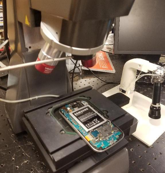
(a) The photograph of our experimental device.

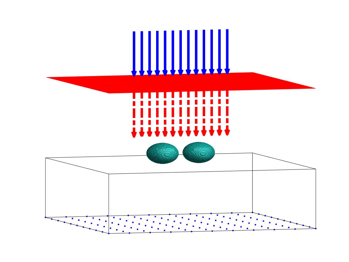
(b) A schematic diagram of data collection.

Figure 3: The data collection setup

As it was stated in Introduction, following the idea of a series of works of experimentalists, such as, e.g. [63], we use the detector array of the camera of Samsung Galaxy S3 cell phone. Figure 3 displays the photograph of our experimental device. We use white light. By using narrow-pass spectral filters, we filtered relatively narrow bands with the width around 10$\mu m$ centered at the different wavelengths ($\lambda$) which were distributed throughout the visible spectrum:

$$\lambda=0420,0.473,0.525,0.580,0.620,0.671\mu m.$$ (6.1)

We have made variables dimensionless via the change of variables in Helmholtz equation (2.6)

$$\mathbf{x}^{\prime}=\frac{\mathbf{x}}{10\mu m}.$$ (6.2)

Then the dimensionless wavelength $\lambda^{\prime}=\lambda/(10\mu m)$ and the wave number $k=2\pi/\lambda^{\prime}.$We keep the same notations for new variables for brevity. Hence, by (6.1) we use the following values of $k$:

$$k=93.6,101.3,108.3,119.7,132.8,149.5.$$ (6.3)

However, as stated in Section 4, we have observed that the data is too noisy for all values of $k$ in (6.3). Only data for wave numbers $108.3$ and $119.7$ have acceptable noise level. Hence, we set as in (4.1) $\underline{k}=108.3,\overline{k}=119.7$. Next, to obtain the data for $\left|u\left(\mathbf{x},k\right)\right|^{2}\mid_{\mathbf{x}\in P_{\text{meas}}}$ for all other values of $k\in\left[\underline{k},\overline{k}\right],$ we have linearly interpolated the measured data between points $k=\underline{k}$ and $k=\overline{k}.$

An array of camera’s photosensitive pixels was covered by the manufacturer with a protective glass layer, as illustrated in Figure 3b. In this glass, the refractive index $n_{0}=1.5$. Thus, we take this value as the refractive index of the background. We must scale the model, so that the value of the refractive index in the background would become $n_{\text{bkgr}}=1$. To do this, we again change variables as

$$\mathbf{y}=n_{0}\mathbf{x},\text{ }\mathbf{x}\in\mathbb{R}^{3}.$$ (6.4)

The Helmholtz equation in (2.6) becomes

$$\Delta_{\mathbf{y}}u(\mathbf{y},k)+k^{2}\left(\frac{n(\mathbf{y})}{n_{0}}\right)^{2}u(\mathbf{y},k)=0.$$

When we solve Problem 5.1 by the above globally convergent method, we find first the relative contrast $n_{\text{rel}},$

$$n_{\text{rel}}=\frac{n}{n_{0}}=\frac{n}{1.5}.\text{ }$$

Next, we find the refractive index as $n=1.5n_{\text{rel}}.$

Below all sizes are those which were made dimensionless first by (6.2) and scaled ones then by (6.4). The value of the dielectric constant in each microsphere of our experiments was

$$n\left(\text{microsphere}\right)=2.15,\text{ }n_{\text{rel}}\left(\text{microsphere}\right)=1.43.$$ (6.5)

In our experiments, we have collected the above mentioned data for the case when scatterers were microspheres of the radius $0.45$. The center of each microsphere was located on the plane $\left\{x_{3}=0\right\}.$ The measurement plane was located at $R=49.5$. We have measured the data at that plane on a square $P_{\text{meas}},$

$$P_{\text{meas}}=\left\{\left|x_{1}\right|,\left|x_{2}\right|<3.75,x_{3}=R=49.5\right\},$$ (6.6)

$$\Omega=\left\{\left|x_{1}\right|,\left|x_{2}\right|<3.75,x_{3}\in\left(6.8,0.7\right)\right\},$$

$$\Gamma=\left\{\left|x_{1}\right|,\left|x_{2}\right|<3.75,x_{3}=0.7\right\}.$$ (6.7)

7 Numerical Results 

In this section, we present our numerical results for solving Problem 2.1 for both computationally simulated and experimental data. First, we have reconstructed the wave field at $P_{\text{meas}}$ using the reconstruction formula (4.21). We reduce Problem 2.1 to Problem 5.1. Next, we have solved the latter problem by the method outlined in Section 5 and have reconstructed the unknown refractive index $n\left(\mathbf{x}\right)$ this way, i.e. we have imaged our microspheres.

We had two sets of experimental data. The first one was for the case of a single microsphere and the second one was for the case of two microspheres. For each case we have solved both phaseless CIPs: one with experimental data and the second one with computationally simulated data. It is important that computationally simulated data were generated for exactly the same values of parameters as those in corresponding microspheres in experiments: we have used exactly the same radii of spheres $0.45$, locations of their centers and values of the relative index $n=2.15$ in (6.5). In all tests, the interval of wave numbers was the sama as in (4.1).

We have performed such tests for computationally simulated data in order to verify our method via the comparison of results with those for experimental data.

We now describe how we modeled our microspheres for computationally simulated data. In order to improve the accuracy of the solution of the forward problem, we have decided to smooth out inclusion/background interface rather than having the function $c\left(\mathbf{x}\right)$ which would have a discontinuity on this interface.

Define the smooth function $\psi\in C^{\infty}(\mathbb{R}^{3})$ as

$$\psi(\mathbf{x})=\left\{\begin{array}[]{ll}\exp\left(-\frac{|\mathbf{x}|^{2}}{1-|\mathbf{x}|^{2}}\right)&|\mathbf{x}|<1\\ 0&|\mathbf{x}|\geq 1.\end{array}\right.$$

Let $\mathbf{x}_{0}$ be the center and $r=0.45$ be the radius of the microsphere used in our simulations. Then, taking into account that by (6.5) $n_{\text{rel}}^{2}\left(\text{microsphere}\right)=2.04$, we use the following function $n^{2}(\mathbf{x})$ in our computational simulations

$$n^{2}(\mathbf{x})=1+1.04\psi\left(\frac{\mathbf{x}-\mathbf{x}_{0}}{r}\right).$$

In the case of two microspheres with their centers at $\mathbf{x}_{0}^{\left(1\right)}$ and $\mathbf{x}_{0}^{\left(2\right)}$ and with the distance between their centers exceeding 1, we have

$$n^{2}(\mathbf{x})=1+1.04\psi\left(\frac{\mathbf{x}-\mathbf{x}_{0}^{\left(1\right)}}{r}\right)+1.04\psi\left(\frac{\mathbf{x}-\mathbf{x}_{0}^{\left(2\right)}}{r}\right).$$

Let $n^{\text{comp}}\left(\mathbf{x}\right),\mathbf{x}\in\overline{\Omega}$ be the computed refractive index $n\left(\mathbf{x}\right).$ As the computed value $n_{\text{comp}}$ of the refractive index $n$ in inclusions, we take:

$$n_{\text{comp}}\left(\text{microsphere}\right)=\max_{\overline{\Omega}}n^{\text{comp}}\left(\mathbf{x}\right).$$ (7.1)

7.1 Test 1: One microsphere

Figure 4 displays the modulus $\left|u\left(\mathbf{x},\underline{k}\right)\right|,\underline{k}=108.3$ of both experimental (a) and computationally simulated (b) data at the measurement square $P_{\text{meas}},$ see (6.6). One can see good agreement between the experimental (left) and computed (right) data. The difference can be ascribed to the noise in the experimental system.

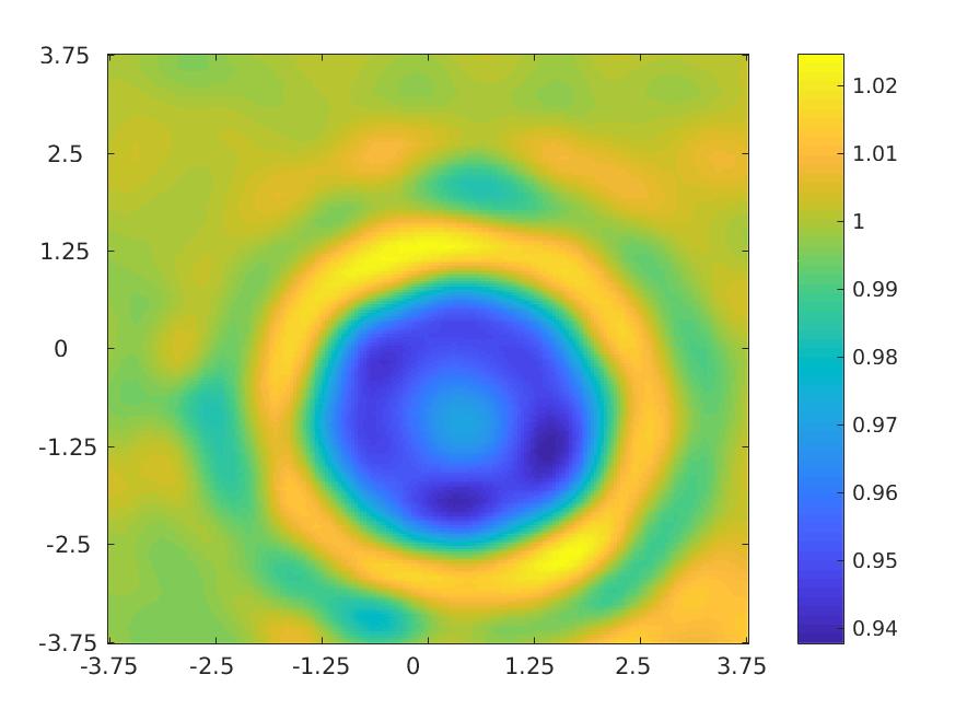
(a) Experimental data.

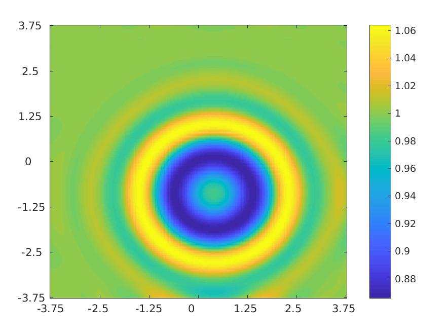
(b) Computationally simulated data.

Figure 4: Test 1. The function $|u({\mathbf{x}},k)|$, ${\mathbf{x}}\in P_{\mathrm{m}eas}$ and $k=119.7$. The similarity of experimental data and the computationally simulated data is evident.

Figure 5 represents the true and reconstructed real and imaginary parts of the function $u\left(\mathbf{x},\underline{k}\right)$ for $\mathbf{x}\in P_{\text{meas}}$ for computationally simulated data. The true function $u\left(\mathbf{x},\underline{k}\right)$ was computed via the numerical solution of equation (2.10). The reconstructed function $u\left(\mathbf{x},\underline{k}\right)$ was computed via the reconstruction formula (4.21). Figures 6 were obtained as follows: we have arranged a uniform $100\times 100$ grid of points $\{\mathbf{x}_{l}\}_{l=1}^{10,000}$ in $P_{\mathrm{meas}}$. So, Figures 6 show true and reconstructed values of $\mathop{\mathrm{R}e}u(\mathbf{x}_{s},\underline{k})$ and $\mathop{\mathrm{I}m}u(\mathbf{x}_{s},\underline{k})$, where $s\in\{7400,\dots,8600\}$. One can see that imaginary parts coincide quite well, whereas real parts coincide sort of satisfactory, given a highly oscillatory behavior of these curves. In addition, using Remark 4.1, we conclude that our reconstruction formulae of Theorem 4.2 are rather accurate ones, especially given a difficult nature of our phaseless CIP.

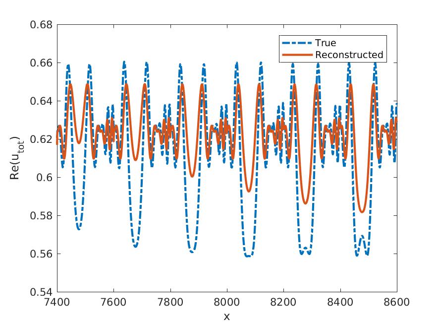
(a) The true and reconstructed real parts of the function $u({\mathbf{x}},k)$

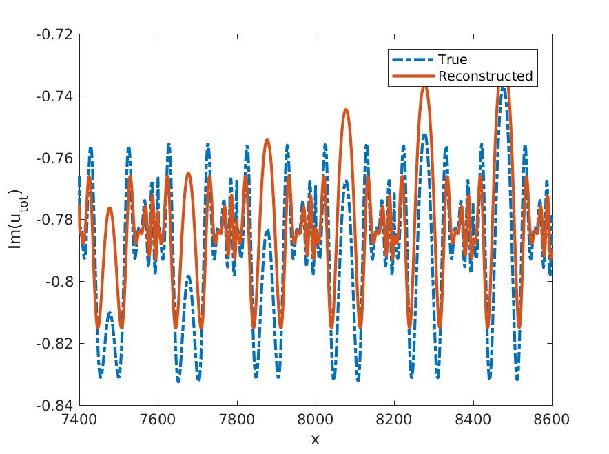
(b) The true and reconstructed imaginary parts of the function $u({\mathbf{x}},k)$

Figure 5: Test 1. The reconstruction of the complex valued function $u({\mathbf{x}},k)$ with $k=119.7$ using the inversion formula (4.21). One can see that imaginary parts coincide quite well, whereas real parts coincide sort of satisfactory, given a highly oscillatory behavior of these curves. We conclude that our reconstruction formula (4.21) is quite accurate.

Figure 6 displays the modulus of $\left|u\left(\mathbf{x},\underline{k}\right)\right|$ for $\mathbf{x}\in\Gamma,$ where $\Gamma\subset\partial\Omega$ was defined in (6.7). In other words, Figures 6 show the modulus of propagated data, both for the experimental and computationally simulated cases. One can see that Figures 6a and 6b look quite similar. In other words, propagated data for these two cases are quite close to each other. One can also see that the data propagation helps to figure out $\left(x_{1},x_{2}\right)$ coordinates of inclusions.

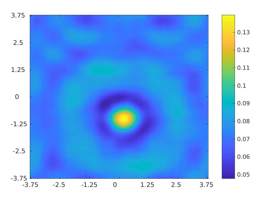
(a) The propagation of experimental data

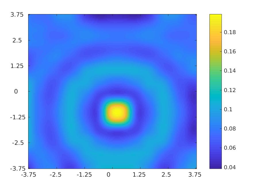
(b) The propagation of simulated data

Figure 6: Test 1. Modulus of the propagated data $|u({\mathbf{x}},k)|$ for ${\mathbf{x}}\in\Gamma$. A good similarity between (a) and (b) is observed. One can also see that the data propagation helps to figure out $(x_{1},x_{2})$ coordinates of inclusions.

Table 1: Test 1. True and computed values of the refractive indices in reconstructed microspheres, see (7.1).

Data	True $n\left(\text{microsphere}\right)$	$n_{\text{comp}}\left(\text{microsphere}\right)$	Relative error
Experimental	2.15	2.043	5.2%
Simulated	2.15	2.04	5.4%

It follows from Table 1 that values of the computed refractive indices of reconstructed microspheres for experimental and simulated data are almost the same. The computational error is quite small in both cases.

Figure 7 displays resulting images. One can see that images for both computationally simulated and experimental data are very similar and also similar with the true image. Thus, locations of inclusions are also correctly reconstructed.

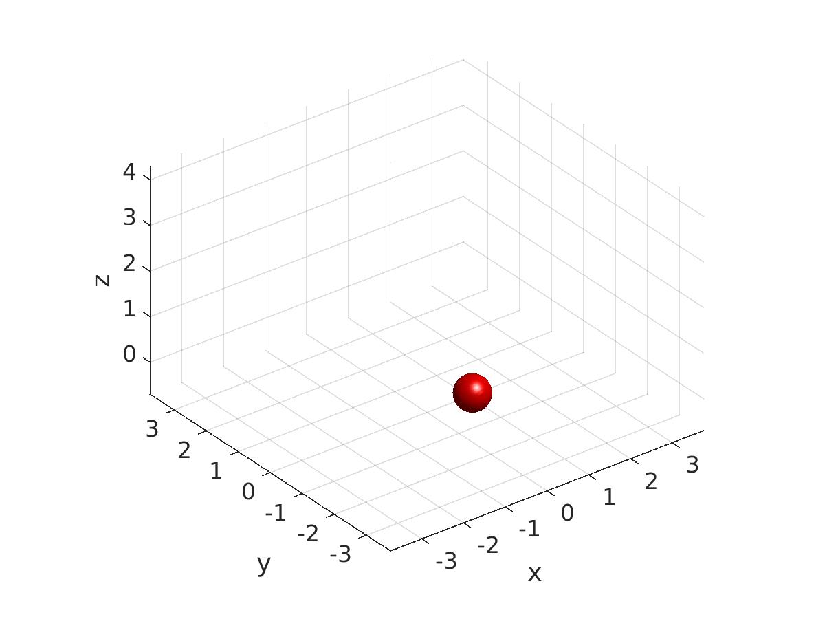
(a) True image

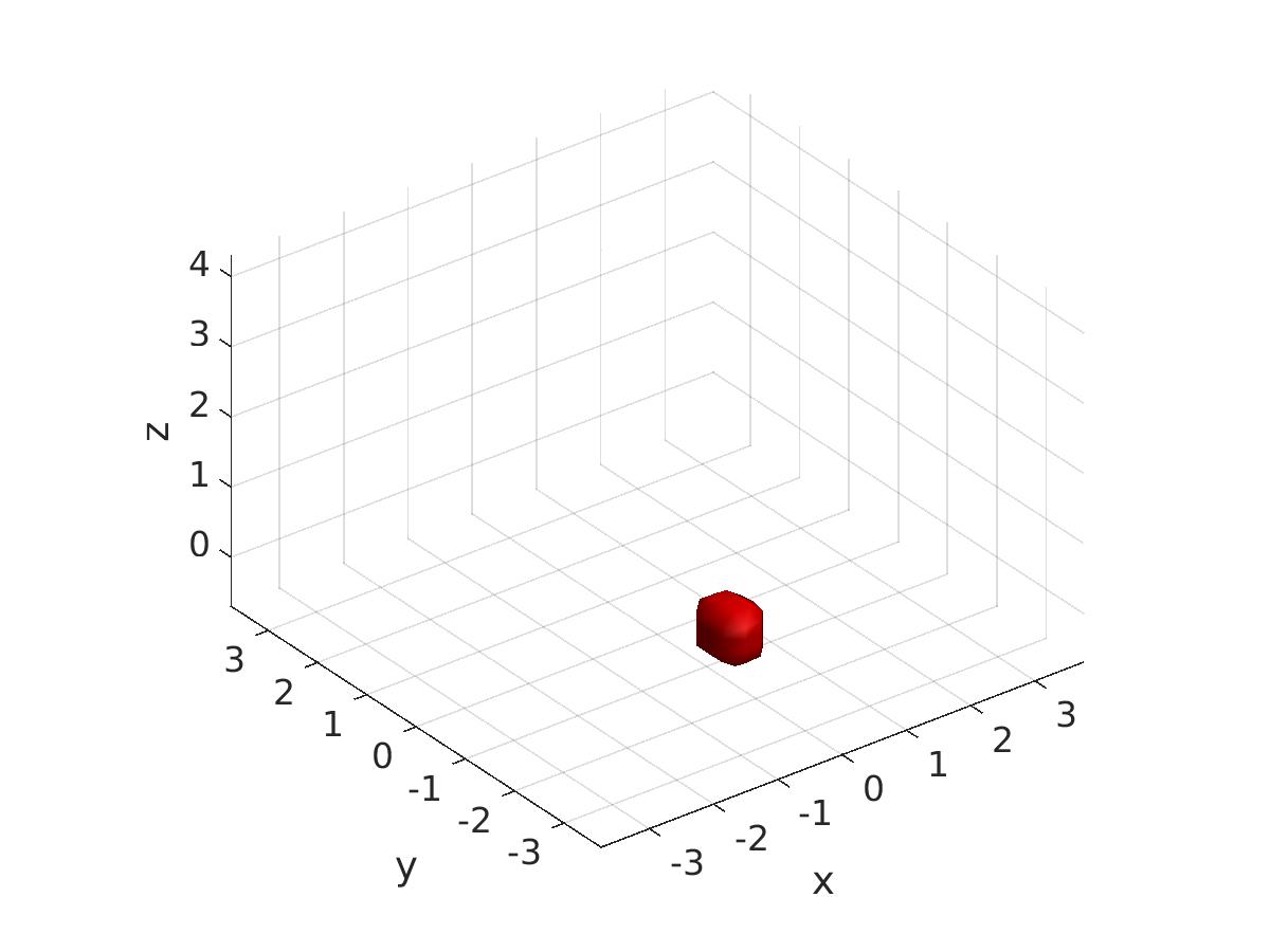
(b) Image computed from simulated data.

(c) Image computed from experimental data.

Figure 7: Test 1. True and computed images of the microsphere involved in the experiment. One can observe that the location of the unknown microsphere is imaged with a very good accuracy in both cases. A similarity between (b) and (c) can also be observed.

7.2 Test 2: Two microspheres

Since results for this case are very similar with ones for the case of one microsphere, we shorten in this section, compared with the previous one. Since the comparison of functions $\mathop{\mathrm{R}e}u(\mathbf{x},\underline{k})$ and $\mathop{\mathrm{I}m}u(\mathbf{x},\underline{k})$ for $\mathbf{x}\in P_{\text{meas}}$ for computationally simulated and experimental data is very similar for this case with Test 1, we do not show here an analog of Figure 5: for brevity. The same for an analog of Figure 6.

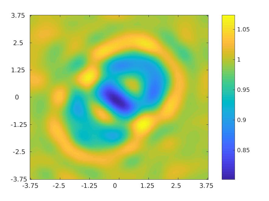
(a) Experimental data

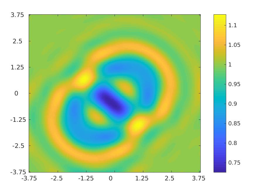
(b) Simulated data

Figure 8: Test 2. The data $|u({\mathbf{x}},k)|$, ${\mathbf{x}}\in P_{\mathrm{m}eas}$ and $k=119.7$.

Table 2: Test 2. Correct and computed values of the refractive indices in two reconstructed microspheres, see (7.1).

Data	Correct $n\left(\text{microsphere}\right)$	$n_{\text{comp}}\left(\text{microsphere}\right)$	Relative error
Experimental	2.15	2.04 (in both microspheres)	5.4%
Simulated	2.15	2.04 (in both microspheres)	5.4%

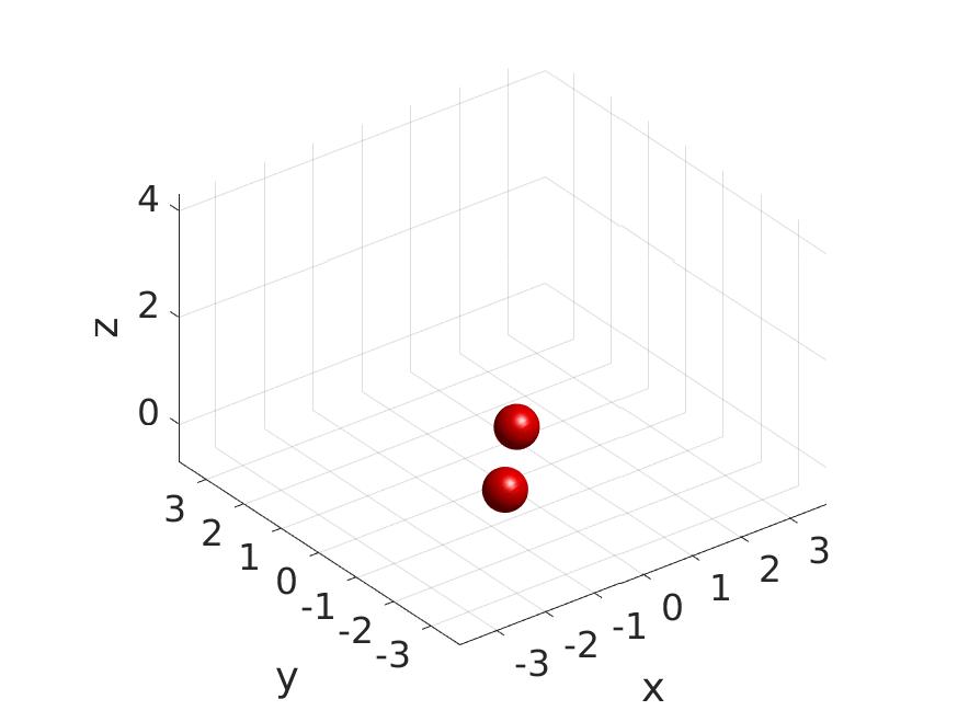
(a) True image

(b) Image computed from simulated data

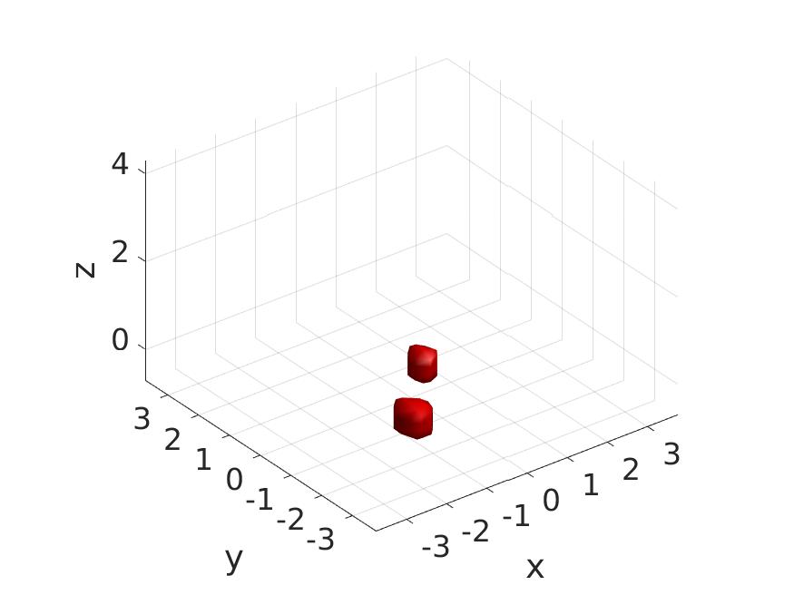
(c) Image computed from experimental data

Figure 9: Test 2. Correct and computed images of two microspheres involved in the experiment. One can observe that the locations of the unknown microspheres are imaged with a very good accuracy in both cases. A close similarity between (b) and (c) can also be observed.

8 Summary

We have collected phaseless scattering data on six (6) wavelengths $\lambda$ listed in (6.1) ranging from $\lambda=0.42\mu m$ to $\lambda=0.671\mu m.$ To obtain the data at these wavelengths from the white light, we have used narrow light filters. But only the data on $\lambda=0.525\mu m$ and $\lambda=0.580\mu m$ turned out to have a reasonable amount of noise. So, we have linearly interpolated the measured data between points $k=\underline{k}=108.3$ and $k=\overline{k}=119.7,$ which mean corresponding wave numbers. Only a single direction of the incident plane wave was used, i.e. we have worked with the phaseless CIP with the data resulting from a single measurement event. This is definitely more challenging than the case of multiple measurements. We have measured the intensity $\left|u\left(\mathbf{x},k\right)\right|^{2}\mid_{P_{\text{meas}}}$of the full complex valued wave field on a square $P_{\text{meas}}$ located on a plane, which is orthogonal to the direction of the propagation of the incident plane wave. Here $u\left(\mathbf{x},k\right)$ is the solution of the Helmholtz equation (2.6) with the radiation condition.

Since previous works on reconstruction procedures for phaseless CIPs [40, 41, 42, 43, 39, 37]of the first author with coauthors have discussed only phaseless CIPs with measurements of $\left|u_{\text{sc}}\left(\mathbf{x},k\right)\right|^{2}$, where $u_{\text{sc}}\left(\mathbf{x},k\right)$ is the scattered wave field, we have developed a new procedure to approximately reconstruct the function $u\left(\mathbf{x},k\right)\mid_{P_{\text{meas}}}$ from its modulus measured on $P_{\text{meas}}.$

One of the key obstacles in this direction was the absence of a proper analytical estimate of $\left|u_{\text{sc}}\left(\mathbf{x},k\right)\right|^{2}.$ While we have observed numerically that this term is small indeed and can be dropped (Figures 2), it was unclear how to prove this analytically. To obtain a proper estimate for this term, we have used Theorems 3.5 and 4.6. Both these theorems use ideas of the Riemannian geometry and asymptotic analysis. While Theorem 3.5 was actually proved in [43], Theorem 4.6 is completely new. As a result, our upper estimate (4.6) of $\left|u_{\text{sc}}\left(\mathbf{x},k\right)\right|^{2}\mid_{P_{\text{meas}}}$is a reasonable one for the given range of parameters. Furthermore, number-wise this estimate is approximately the same as purely numerical estimates of Figures 2. Thus, the analytical estimate (4.6) in combination with Figures 2 ensure that the term $\left|u_{\text{sc}}\left(\mathbf{x},k\right)\right|^{2}\mid_{P_{\text{meas}}}$ is sufficiently small compared with 1. Hence, this term can be dropped in (4.15). The resulting formula (4.16), in combination with Theorem 3.5, enables us to obtain the inversion formula (4.21).

As soon as the function $u\left(\mathbf{x},k\right)\mid_{P_{\text{meas}}}$ is approximately reconstructed, one obtains the conventional phased CIP, which, however, is also difficult to solve. Its numerical solution is the second stage of our reconstruction procedure. To solve this problem numerically, we have used the globally convergent numerical method which was developed in [38] and then successfully tested on microwave backscattering experimental data in [46, 54, 53].

In our numerical studies we have decided to verify the accuracy of our inversions of experimental data via comparison of inversion results with those of computationally simulated data. Thus, we have computationally generated the data for exactly the same microspheres as we have used in experiments. We have observed that computational results for the forward problem have a very good similarity with experimental data, see Figures 4, 5, 8. In addition, inversion results for both experimental data sets are very similar with the those of computationally simulated data, see Figures 6, 7, 9 and Tables 1,2. Finally, the reconstruction  error of the refractive index is between 5.2% and 5.4% in all cases, which is small.

Thus, we conclude that since results of the forward problem solution for computationally simulated data are quite close to the experimental data and also since our inversion provides quite accurate locations and refractive indices of microspheres of interest for both types of data, then our mathematical modeling of experimental data is quite accurate one, including the drop of the term $\left|u_{\text{sc}}\left(\mathbf{x},k\right)\right|^{2}\mid_{P_{\text{meas}}}$ in (4.15).

Acknowledgements

The work of M. V. Klibanov and N. A. Koshev was supported by the US Army Research Laboratory and US Army Research Office grant W911NF-15-1-0233 as well as by the Office of Naval Research grant N00014-15-1-2330. The work of L. H. Nguyen was partially supported by research funds FRG 111172 provided by University of North Carolina at Charlotte.

References

- [1] T. Aktosun and P. Sacks. Inverse problem on the line without phase information. Inverse Problems, 14 (2):211–224, 1998.
- [2] H. Ammari, Y. Chow, and J. Zou. Phased and phaseless domain reconstruction in inverse scattering problem via scattering coefficients. SIAM Journal on Applied Mathematics, 76:1000–1030, 2016.
- [3] H. Ammari, Y.T. Chow, and J. Zou. The concept of heterogeneous scattering and its applications in inverse medium scattering. SIAM Journal on Mathematical Analysis, 46:2905–2935, 2014.
- [4] H. Ammari, J. Garnier, W. Jing, H. Kang, M. Lim, K. Sølna, and H. Wang. Mathematical and Statistical Methods for Multistatic Imaging. Springer, 2013.
- [5] G. Bao, P. Li, and J. Lv. Numerical solution of an inverse diffraction grating problem from phaseless data. Journal of the Optical Society of America, 30:293–299, 2013.
- [6] G. Bao and L. Zhang. Shape reconstruction of the multi-scale rough surface from multi-frequency phaseless data. Inverse Problems, 32(8):0850002, 2016.
- [7] P. Bardsley and F. Guevar. Vasquez. Imaging with power controlled source pairs. SIAM Journal of Imaging Sciences, 9:185–211, 2016.
- [8] P. Bardsley and F.Guevara Vasquez. Kirchhoff migration without phases. Inverse Problems, 32:105006, 2016.
- [9] L. Baudouin, M. de Buhan, and S. Ervedoza. Convergent algorithm based on Carleman estimates for the recovery of a potential in the wave equation. SIAM Journal on Numerical Analysis, 55:1578–1613, 2017.
- [10] L. Beilina and M.V. Klibanov. Approximate Global Convergence and Adaptivity for Coefficient Inverse Problems. Springer, New York, 2012.
- [11] M. Bellassoued and M. Yamamoto. Carleman Estimates and Applications to Inverse Problems for Hyperbolic Systems. Springer Japan KK, 2017.
- [12] A. L. Bukhgeim and M. V. Klibanov. Global uniqueness of a class of multidimensional inverse problems. Soviet Math Dokl., 24:244–247, 1981.
- [13] S. Bürger, J. Flemming, and B. Hofmann. On complex-valued deautoconvolution of compactly supported functions with sparse Fourier representation. Inverse Problems, 32:104006, 2016.
- [14] S. Bürger and B. Hofmann. About a deficit in low-order convergence rates on the example of autoconvolution. Applicable Analysis, 94:477–493, 2015.
- [15] K. Chadan and P. Sabatier. Inverse Problems in Quantum Scattering Theory. Springer-Verlag, New York, 1977.
- [16] Y.T. Chow and J. Zou. A numerical method for reconstructing the coefficient in a wave equation. Numericall Methods for Partial Differential Equations, 31:289–307, 2015.
- [17] D. Colton and R. Kress. Inverse acoustic and electromagnetic scattering theory. Springer, New York, 3rd edition, 2013.
- [18] D. Gerthab, B. Hofmann, S. Birkholzc, S. Kokec, and G. Steinmeyer. Regularization of an autoconvolution problem in ultrashort laser pulse characterization. Inverse Problems of Science and Engineering, 22:245–266, 2014.
- [19] A.V. Goncharsky and S.Y. Romanov. Supercomputer technologies in inverse problems of ultrasound tomography. Inverse Problems, 29:075004, 2013.
- [20] A.V. Goncharsky and S.Y. Romanov. Iterative methods for solving coefficient inverse problems of wave tomography in models with attenuation. Inverse Problems, 33 (2):025003, 2017.
- [21] F. Hecht. New development in Freefem++. Journal of Numerical Mathematics, 20:251–266, 2012.
- [22] K. Ito, B. Jin, and J. Zou. A direct sampling method for inverse electromagnetic medium scattering. Inverse Problems, 29:095018, 2013.
- [23] O. Ivanyshyn and R. Kress. Identification of sound-soft 3D obstacles from phaseless data. Inverse Problems and Imaging, 4:131–149, 2010.
- [24] O. Ivanyshyn and R. Kress. Inverse scattering for surface impedance from phaseless far field data. Journal of Computational Physics, 230:3443–3452, 2011.
- [25] O. Ivanyshyn, R. Kress, and P. Serranho. Huygens’ principle and iterative methods in inverse obstacle scattering. Advances in Computational Mathematics, 33:413–429, 2010.
- [26] S.I. Kabanikhin, N.S. Novikov, I.V. Osedelets, and M. Shishlenin. Fast Toeplitz linear system inversion for solving two-dimensional acoustic inverse problem. Journal of Inverse and Ill-Posed Problems, 23:687–700, 2015.
- [27] S.I. Kabanikhin, K.K. Sabelfeld, N.S. Novikov, and M.A. Shishlenin. Numerical solution of the multidimensional Gelfand-Levitan equation. Journal of Inverse and Ill-Posed Problems, 23:439–450, 2015.
- [28] S.I. Kabanikhin, A.D. Satybaev, and M. Shishlenin. Direct Methods of Solving Multidimensional Inverse Hyperbolic Problem. VSP, Utrecht, 2004.
- [29] M.V. Klibanov. On the recovery of a 2-D function from the modulus of its fourier transform. Journal of Mathematical Analysis and Applications, 323:818–843, 2006.
- [30] M.V. Klibanov. Carleman estimates for global uniqueness, stability and numerical methods for coefficient inverse problems. Journal of Inverse and Ill-Posed Problems, 21:477–560, 2013.
- [31] M.V. Klibanov. On the first solution of a long standing problem: Uniqueness of the phaseless quantum inverse scattering problem in 3-d. Applied Mathematics Letters, 37:82–85, 2014.
- [32] M.V. Klibanov. Phaseless inverse scattering problems in three dimensions. SIAM Journal on Applied Mathematics, 74:392–410, 2014.
- [33] M.V. Klibanov. Uniqueness of two phaseless non-overdetermined inverse acoustics problems in 3-d. Applicable Analysis, 93:1135–1149, 2014.
- [34] M.V. Klibanov. A phaseless inverse scattering problem for the 3-D Helmholtz equation. Inverse Problems and Imaging, 11:263–276, 2017.
- [35] M.V. Klibanov and V.G. Kamburg. Uniqueness of a one-dimensional phase retrieval problem. Inverse Problems, 30:075004, 2014.
- [36] M.V. Klibanov, A.E. Kolesov, L. Nguyen, and A. Sullivan. Globally strictly convex cost functional for a 1-D inverse medium scattering problem with experimental data. SIAM Journal on Applied Mathematics, 77:1733–1755, 2017.
- [37] M.V. Klibanov, D.-L. Nguyen, and L.H. Nguyen. A coefficient inverse problem with a single measurement of phaseless scattering data. 2017.
- [38] M.V. Klibanov, D.-L. Nguyen, L.H. Nguyen, and H. Liu. A globally convergent numerical method for a 3d coefficient inverse problem with a single measurement of multi-frequency data. to appear in Inverse Problems and Imaging, 2017.
- [39] M.V. Klibanov, L.H. Nguyen, and K. Pan. Nanostructures imaging via numerical solution of a 3-D inverse scattering problem without the phase information. Applied Numerical Mathematics, 110:190–203, 2016.
- [40] M.V. Klibanov and V.G. Romanov. Explicit formula for the solution of the phaseless inverse scattering problem of imaging of nano structures. Journal of Inverse and Ill-Posed Problems, 23:187–193, 2015.
- [41] M.V. Klibanov and V.G. Romanov. Explicit solution of 3-d inverse scattering problem for the Schrödinger equation: the plane wave case. Eurasian Journal of Mathematical and Computer Applications, 3:48–63, 2015.
- [42] M.V. Klibanov and V.G. Romanov. Reconstruction procedures for two inverse scattering problems without the phase information. SIAM Journal on Applied Mathematics, 76:178–196, 2016.
- [43] M.V. Klibanov and V.G. Romanov. Two reconstruction procedures for a 3d phaseless inverse scattering problem for the generalized Helmholtz equation. Inverse Problems, 32:015005, 2016.
- [44] M.V. Klibanov and V.G. Romanov. Uniqueness of a 3-D coefficient inverse scattering problem without the phase information. Inverse Problems, 33:095007, 2017.
- [45] M.V. Klibanov and P. Sacks. Phaseless inverse scattering and the phase problem in optics. Journal of Mathematical Physics, 33:3813–3821, 1992.
- [46] A.E. Kolesov, M.V. Klibanov, L.H. Nguyen, D.-L. Nguyen, and N.T. Thành. Single measurement experimental data for an inverse medium problem inverted by a multi-frequency globally convergent numerical method. Applied Numerical Mathematics, 120:176–196, 2017.
- [47] A. Lakhal. A decoupling-based imaging method for inverse medium scattering for Maxwell’s equations. Inverse Problems, 26:015007, 2010.
- [48] A. Lechleiter and D.-L. Nguyen. A trigonometric Galerkin method for volume integral equations arising in TM grating scattering. Advances in Computational Mathematics, 40:1–25, 2014.
- [49] J. Li, P. Li, H. Liu, and X. Liu. Recovering multiscale buried anomalies in a two-layered medium. Inverse Problems, 31:105006, 2015.
- [50] J. Li, H. Liu, and Q. Wang. Enhanced multilevel linear sampling methods for inverse scattering problems. Journal of Computational Physics, 257:554–571, 2014.
- [51] J. Li, H. Liu, and Y. Wang. Recovering an electromagnetic obstacle by a few phaseless backscattering measurements. Inverse Problems, 33:035011, 2017.
- [52] D.-L. Nguyen. A volume integral equation method for periodic scattering problems for anisotropic Maxwell’s equations. Applied Numerical Mathematics, 98:59–78, 2015.
- [53] D.-L. Nguyen, M.V. Klibanov, L.H. Nguyen, and M.A. Fiddy. Imaging of buried objects from multi-frequency experimental data using a globally convergent inversion method. Inverse and Ill-posed Problems, https://doi.org/10.1515/jiip-2017-0047, 2017.
- [54] D.-L. Nguyen, M.V. Klibanov, L.H. Nguyen, A.E. Kolesov, M.A. Fiddy, and H. Liu. Numerical solution of a coefficient inverse problem with multi-frequency experimental raw data by a globally convergent algorithm. Journal of Computational Physics, 345:17–32, 2017.
- [55] L. Novotny and B. Hecht. Principles of Nano-Optics. Cambridge University Press, Cambridge, UK, 2 edition, 2012.
- [56] T. Petersena, V. Keastb, and D. Paganinc. Quantitative TEM-based phase retrieval of MgO nano-cubes using the transport of intensity equation. Ultramisroscopy, 108:805–815, 2008.
- [57] R. Phillips and R. Milo. A feeling for numbers in biology. In PNAS-USA, volume 106, pages 21465–21471. Academy of Sciences USA, 2009.
- [58] V.G. Romanov. Inverse Problems of Mathematical Physics. VSP, Utrecht, 1986.
- [59] V.G. Romanov. Investigation Methods for Inverse Problems. VSP, Utrecht, 2002.
- [60] V.G. Romanov. Inverse problems for differential equations with memory. Eurasian J. Math. Comput. Appl., 2:51–80, 2013.
- [61] V.G. Romanov and M. Yamamoto. Phaseless inverse problems with interference waves. arXiv:1801.10062, 2018.
- [62] A. Ruhlandt, M. Krenkel, M. Bartels, and T. Salditt. Three-dimensional phase retrieval in propagation-based phase-contrast imaging. Phys. Rev. A, 89:033847, 2014.
- [63] D. Tseng, O. Mudanyali, C. Oztoprak, S.O. Isikman, I. Sencan, O. Yagliderea, and A. Ozcan. Lensfree microscopy on a cellphone. Lab Chip., 10:1787–1792, 2010.