Inflationary perturbations with Lifshitz scaling

Abstract:

Instead of Lorentz invariance, gravitational degrees of freedom may obey Lifshitz scaling at high energies, as it happens in Hořava’s proposal for quantum gravity. We study consequences of this proposal for the spectra of primordial perturbations generated at inflation. Breaking of 4D diffeomorphism (Diff) invariance down to the foliation-preserving Diff in Hořava-Lifshitz (HL) gravity leads to appearance of a scalar degree of freedom in the gravity sector, khronon, which describes dynamics of the time foliation. One can naively expect that mixing between inflaton and khronon will jeopardize conservation of adiabatic perturbations at super Hubble scales. This indeed happens in the projectable version of the theory. By contrast, we find that in the non-projectable version of HL gravity, khronon acquires an effective mass which is much larger than the Hubble scale well before the Hubble crossing time and decouples from the adiabatic curvature perturbation $\zeta$ sourced by the inflaton fluctuations. As a result, at super Hubble scales the adiabatic perturbation $\zeta$ behaves as in an effectively single field system and its spectrum is conserved in time. Lifshitz scaling is imprinted in the power spectrum of $\zeta$ through the modified dispersion relation of the inflaton. We point out violation of the consistency relation between the tensor-to-scalar ratio and the spectral tilt of primordial gravitational waves and suggest that it can provide a signal of Lorentz violation in inflationary era.

1 Introduction

General relativity (GR) accurately describes all known gravitational phenomena. Still, it has a theoretical flaw: it is not renormalizable [1] and thus cannot be a complete theory of quantum gravity. One way to address this problem is to introduce terms with higher powers of the curvature tensor which make the theory renormalizable [2]. However, if Lorentz invariant, these higher curvature terms lead to loss of unitarity. This motivated P. Hořava to propose a framework to render gravity power-counting renormalizable by abandoning Lorentz invariance [3]. By breaking Lorentz invariance, we can introduce higher spatial derivative terms, while avoiding higher time derivative terms and thus making the theory compatible with unitarity. A key role in the power-counting argument is played by an approximate invariance of the theory at high energies and momenta with respect to the so-called Lifshitz scaling transformations. These stretch space and time by different amount, so they are also often referred to as anisotropic scaling. The dispersion relations of various degrees of freedom at high energies, compatible with anisotropic scaling, have the form $\omega\propto p^{z}/M_{*}^{z-1}$, where $\omega$ and $p$ are particle’s energy and momentum, $z$ is the Lifshitz exponent ($z$ equals the number of spatial dimensions in Hořava’s proposal) and $M_{*}$ is the energy threshold, above which the anisotropic scaling sets in. This framework has received the name of Hořava–Lifshitz (HL) gravity and the so-called projectable subclass of the resulting theories has been rigorously demonstrated to be perturbatively renormalizable [4, 5]. Moreover, in 2 spatial and 1 time dimensions the theory exhibits asymptotic freedom [6] which strongly suggests that it is ultraviolet (UV) complete.

Deviations from Lorentz invariance are tightly constrained in the Standard Model sector [7, 8, 9]. In the gravity sector constraints come from observations at low energies such as Solar System tests [9, 10], pulsar timing [11, 12, 13, 14], cosmology [15, 16, 17, 18, 19, 20, 21] and direct detection of the gravitational waves [22, 23, 24, 25]. By contrast, Lorentz violation (LV) in the gravity sector is poorly constrained at high energies where it is motivated by renormalization of gravity.

In order to examine the consequences of LV at high energies we study in this paper its effect on cosmic inflation in the early universe. One may expect that breaking of Lorentz invariance during inflation will leave an imprint on the primordial perturbations generated during inflation. This possibility has been explored in a number of works [26, 27, 28, 29, 30, 31, 32, 33, 34, 35]. In HL gravity, where 4D diffeomorphism (Diff) is reduced to foliation preserving Diff, there appears a scalar degree of freedom in gravity sector, so called khronon. It is tempting to speculate that this additional degree of freedom can play the role of inflaton. However, at the moment this seems to be forbidden due the restrictive symmetry structure of the theory. Therefore, to drive inflation, we need to introduce a scalar field, as usual. Then, in general, generation of the primordial scalar perturbation is described by a coupled system for two fields, the inflaton and khronon perturbations.

To provide a prediction of the observable quantities, we need to solve consistently the two field system of the inflaton and khronon, which are coupled with each other during inflation. When 4D Diff is preserved and the universe is dominated by a single component, it is well-known that the adiabatic curvature perturbation $\zeta$ stays constant in time after the Hubble crossing (see, e.g., Refs. [36, 37]). On the other hand, in HL gravity the number of scalar degrees of freedom is always greater than one due to the presence of khronon and it is not clear a priori if there exists a conserved variable or not.

The inflaton and khronon are gravitationally coupled even in the absence of a direct interaction between them. In this paper we compute the primordial power spectra by consistently solving the two field models with the inflaton and khronon. The previous studies mostly focused on the regime where the Hubble scale of inflation is low, $H<M_{*}$, so that the higher derivative terms in the action are unimportant and the theory is described by its infrared (IR) limit. By contrast, in this paper we are interested in the high-energy regime of Lifshitz scaling relevant for the case $H>M_{*}$. We consider both projectable and non-projectable versions of HL gravity. As discussed in Refs. [38, 39], the khronon sector of the projectable HL gravity suffers from either the gradient instability or the strong coupling in the IR limit. This means that it cannot describe the physics all the way down to low energies, unless inflationary epoch is separated from the later hot universe by a phase transition that eliminates khronon from the spectrum. Still, the projectable version is perfectly well-behaved in the high-energy regime and its study is instructive to make comparison with the non-projectable version.

When the fluctuations are deep inside the Hubble scale, the gravitational interaction is suppressed and we simply have two decoupled Lifshitz scalars. On the other hand, in the super Hubble scales, the gravitational interaction makes the inflaton and khronon coupled. Then one may naively expect that the primordial spectrum will depend on the time evolution of these two fields and we will need to solve the evolution all along also after the Hubble crossing time. Indeed, this is the case for the projectable version. On the other hand, in the non-projectable version, we will find that khronon gets decoupled from the adiabatic curvature perturbation $\zeta$. As a result, $\zeta$ is conserved at large scales and the power spectrum of $\zeta$ is solely determined by the inflaton. Thanks to the presence of the conserved quantity, we can easily calculate the spectrum of the fluctuation at the end of inflation. Then the consequence of the LV in the spectrum of $\zeta$ only stems from the modification of the dispersion relation.

The spectrum of primordial gravitational waves in HL gravity was computed in Ref. [27]. Once the scalar perturbation is obtained, we can also compute the tensor to scalar ratio $r$. In a 4D Diff invariant theory, there exists a universal relation between $r$ and the tensor spectral tilt $n_{t}$, the so-called consistency relation. We will show that this consistency relation can be broken if the primordial perturbations are generated in the anisotropic scaling regime. The violation of the consistency relation provides a signal of LV in the gravity sector in the high energy regime.

This paper is organized as follows. In Sec. 2 we describe our setup and review the computation of the power spectrum of the Lifshitz scalar and the gravitational waves generated in the anisotropic scaling regime. In Sec. 3 we discuss the behaviour of the khronon perturbation. We show that khronon stays gapless in the projectable version, while it is gapped in the non-projectable version, which leads to the decoupling from the adiabatic mode. In Sec. 4 we discuss violation of the consistency relation by inflationary perturbations with Lifshitz scaling. We conclude in Sec. 5. Appendices summarize some technical details.

2 Primordial perturbations with anisotropic scaling

In this section we describe our setup and briefly summarize the computation of the primordial spectra of the Lifshitz scalar and gravitational waves.

2.1 Projectable and non-projectable Hořava gravity

2.1.1 Lagrangian densities

First, we consider the non-projectable version of HL gravity [3] with the extension introduced in [40]. Due to the complexity of the most general Lagrangian in this framework, we restrict only to the terms that contribute to the action at quadratic order in the perturbations around spatially flat backgrounds and that preserve the parity invariance. This restriction is sufficient to capture the qualitative features of the theory. The complete list of these terms is given in [40] and leads to the following Lagrangian density,

$${\cal L}_{HG}=N\sqrt{h}\bigg{\{} \frac{M_{*}^{2}}{2}\bigg{[}\frac{1}{\alpha_{1}}K_{ij}K^{ij}-\frac{1}{\alpha_{2}}K^{2}+\frac{1}{\alpha_{3}}R+a_{i}a^{i}\bigg{]}$$ (1)

$$-\frac{1}{2}\bigg{[}\frac{R_{ij}R^{ij}}{\beta_{1}}+\frac{R^{2}}{\beta_{2}}-\frac{R\nabla_{i}a^{i}}{\beta_{3}}+\frac{a_{i}\Delta a^{i}}{\beta_{4}}\bigg{]}$$ (2)

$$-\frac{1}{2M_{*}^{2}}\bigg{[}\frac{(\nabla_{i}R_{jk})^{2}}{\gamma_{1}}+\frac{(\nabla_{i}R)^{2}}{\gamma_{2}}+\frac{\Delta R\nabla_{i}a^{i}}{\gamma_{3}}-\frac{a_{i}\Delta^{2}a^{i}}{\gamma_{4}}\bigg{]}\bigg{\}},$$ (3)

where we used the ADM line element, given by

$${\rm d}s^{2}=(N^{2}-N_{i}N^{i}){\rm d}t^{2}-2N_{i}{\rm d}t{\rm d}x^{i}-h_{ij}{\rm d}x^{i}{\rm d}x^{j}\,.$$ (4)

Here $R_{ij}$, $\nabla_{i}$ and $\Delta$ denote the 3-dimensional Ricci tensor, the covariant derivative with respect to $h_{ij}$ and the covariant Laplacian,

$$K_{ij}=\frac{\dot{h}_{ij}-\nabla_{i}N_{j}-\nabla_{j}N_{i}}{2N}$$ (5)

is the extrinsic curvature and we have defined $a_{i}$ as

$$a_{i}\equiv\frac{\partial_{i}N}{N}\,.$$ (6)

Note that we included the integration measure in the definition of the Lagrangian density. The terms in the first line of Eq. (3) describe the low energy part of the action, and the parameters entering it are constrained by the present-day observations. The relation between these parameters and the parameters $\alpha,\lambda,\xi$ introduced in [39] is

$$M_{*}^{2}=M_{P}^{2}\alpha\;,~{}~{}\alpha_{1}=\alpha\;,~{}~{}\alpha_{2}=\alpha/\lambda\;,~{}~{}\alpha_{3}=\alpha/\xi\;,$$ (7)

where $M_{P}$ is the Planck mass. In what follows, we will write

$$\alpha_{1}-\alpha_{2}=2\alpha_{1}\bar{\alpha}\,.$$ (8)

We also discuss the projectable version, where the lapse function is postulated to be space-independent,

$$N=N(t)\,.$$ (9)

The action for the projectable version can be obtained simply by dropping the perturbation of the lapse function in the action for the non-projectable version. Then the parameters $\beta_{3}$, $\beta_{4}$, $\gamma_{3}$, and $\gamma_{4}$ are irrelevant in the projectable theory.

For both the non-projectable and projectable versions, we add as the inflaton a Lifshitz scalar field whose Lagrangian density is given by:

$${\cal L}_{inf}=N\sqrt{h}\biggl{\{}\frac{(\dot{\Phi}-N^{i}\partial_{i}\Phi)^{2}}{2N^{2}}-\frac{\varkappa_{1}}{2}\nabla_{i}\Phi\nabla^{i}\Phi-\frac{\varkappa_{2}}{2M_{*}^{2}}\nabla_{i}\nabla_{j}\Phi\nabla^{i}\nabla^{j}\Phi$$ (10)

$$\qquad\qquad\qquad\qquad-\frac{\varkappa_{3}}{2M_{*}^{4}}\nabla_{i}\nabla_{j}\nabla_{k}\Phi\nabla^{i}\nabla^{j}\nabla^{k}\Phi-V(\Phi)\biggr{\}}\;.$$ (11)

In principle, the coefficients $\varkappa_{1,2,3}$ here can be functions of the field $\Phi$ which has zero scaling dimension. We concentrate on the case of constant coefficients for simplicity. We assume that the inflaton is minimally coupled to the gravity sector. We will briefly discuss a non-minimally coupled case in Sec. 5.

2.1.2 Parameter hierarchy

The Lagrangian density (3) contains a number of parameters. Here we discuss the hierarchy between them. Stability and constraints on deviations from Lorentz invariance at low energies require [39],

$$0<\alpha_{1}\ll 1\,.$$ (12)

Consider now the propagation of gravitational waves in flat spacetime where their dispersion relation is given by

$$\omega^{2}(p)=p^{2}\,\sum_{z=1}^{3}\varkappa_{\gamma,z}\left(\frac{p}{M_{*}}\right)^{2(z-1)}\,,$$ (13)

with

$$\varkappa_{\gamma,1}\equiv\frac{\alpha_{1}}{\alpha_{3}}\,,\qquad\varkappa_{\gamma,2}\equiv\frac{\alpha_{1}}{\beta_{1}}\,,\qquad\varkappa_{\gamma,3}\equiv\frac{\alpha_{1}}{\gamma_{1}}\,.$$ (14)

The coefficient $\varkappa_{\gamma,1}$ determines (the square of) the propagation speed of the gravitational waves at low energies. According to the constraints from the observation of the Hulse-Taylor pulsar [14] and more directly from the detections of the gravitational waves at the two detector sites [22], the propagation speed of the gravitational waves in the IR should be of order of the speed of light, which imposes $\alpha_{1}\simeq\alpha_{3}$. The recent detections of GW170817 and GRB170817A give a tight constraint $|\varkappa_{\gamma,1}-1|<10^{-15}$ [24]. (See also Ref. [41] for the constraint on the subluminal propagation of the gravitational waves from the absence of the gravitational Cherenkov radiation.) Next, requiring that the transition from linear dispersion relation to the Lifshitz scaling happens at $p\sim M_{*}$ we obtain the requirements $\varkappa_{\gamma,2},\varkappa_{\gamma,3}\simeq 1$. By combining these two conditions, we obtain

$$\alpha_{1}\simeq\alpha_{3}\simeq\beta_{1}\simeq\gamma_{1}\ll 1\,.$$ (15)

Let us now turn to khronon. In the projectable version its dispersion relation reads,

$$\omega_{pr}^{2}(p)=\frac{\alpha_{1}\bar{\alpha}}{1+\bar{\alpha}}p^{2}\left[-\frac{1}{\alpha_{3}}+\biggl{(}\frac{3}{\beta_{1}}+\frac{8}{\beta_{2}}\biggr{)}\biggl{(}\frac{p}{M_{*}}\biggr{)}^{2}+\biggl{(}\frac{3}{\gamma_{1}}+\frac{8}{\gamma_{2}}\biggr{)}\biggl{(}\frac{p}{M_{*}}\biggr{)}^{4}\right]\,.$$ (16)

The first term in the square brackets is negative and is responsible for gradient instability in IR. On the other hand, the remaining terms in (16) can be chosen positive, so that at $p>M_{*}$ the dispersion relation is well-behaved. Again, setting the transition to Lifshitz scaling at around $p\simeq M_{*}$ and taking into account (15) we obtain

$$\alpha_{1,3}\simeq\beta_{1,2}\simeq\gamma_{1,2}\ll 1\,.$$ (17)

Further requiring that the overall magnitude of the frequency $\omega_{pr}(p)$ in UV is ${\cal O}(p^{z}/M_{*}^{z-1})$ we set $\bar{\alpha}\simeq{\cal O}(1)$. To sum up, in the projectable case we will work under the assumptions,

$$\alpha_{1,2,3}\simeq\beta_{1,2}\simeq\gamma_{1,2}\ll 1\,,\qquad\bar{\alpha}={\cal O}(1)\qquad\qquad\text{(projectable).}$$ (18)

In the non-projectable version, the dispersion relation for khronon becomes more complicated and is given by

$$\omega_{npr}^{2}(p)=\omega_{pr}^{2}(p)+\frac{2\alpha_{1}\bar{\alpha}}{1+\bar{\alpha}}\,p^{2}\,\frac{\left[-\frac{1}{\alpha_{3}}+\frac{1}{\beta_{3}}(\frac{p}{M_{*}})^{2}+\frac{1}{\gamma_{3}}(\frac{p}{M_{*}})^{4}\right]^{2}}{1+\frac{1}{\beta_{4}}(\frac{p}{M_{*}})^{2}+\frac{1}{\gamma_{4}}(\frac{p}{M_{*}})^{4}}\;,$$ (19)

where the second piece comes from integrating out the lapse function $N$ which enters into the action without time derivatives. Setting the transition scale at $p\simeq M_{*}$ and using Eq. (15), we obtain

$$\alpha_{1,3}\simeq\beta_{1,2,3}\simeq\gamma_{1,2,3}\ll 1\,,\qquad\beta_{4}\simeq\gamma_{4}={\cal O}(1)\,.$$ (20)

Similarly to the discussion of the projectable version, we assume that $\omega(p)$ becomes ${\cal O}(p^{z}/M_{*}^{z-1})$ in UV and obtain

$$\bar{\alpha}\simeq\gamma_{3}^{2}/\alpha_{1}\ll 1\,.$$ (21)

Notice that the order of $\bar{\alpha}$ in the non-projectable version is different from the one in the projectable version, cf. Eq. (18). Combining all conditions together, we obtain

$$\alpha_{1,2,3}\simeq\beta_{1,2,3}\simeq\gamma_{1,2,3}\simeq\bar{\alpha}\ll 1\,,\qquad\beta_{4}\simeq\gamma_{4}={\cal O}(1)\qquad\qquad\text{(non-projectable).}$$ (22)

The parameters which satisfy these conditions are consistent with the experimental data in IR [39].

2.2 Background equations

Equations for the inflationary background read,

$$3M_{P}^{2}\frac{1+\bar{\alpha}}{1-2\bar{\alpha}}H^{2}=\frac{\dot{\phi}^{2}}{2}+V\,,$$ (23)

$$\ddot{\phi}+3H\dot{\phi}+V_{\phi}=0\,,$$ (24)

where $\phi$ is the background value of the inflaton and $V_{\phi}$ denotes the derivative of $V$ with respect to $\phi$. Positivity of the l.h.s. in the Friedmann equation (23) requires $\bar{\alpha}$ to be in the range $-1<\bar{\alpha}<1/2$. We define the slow-roll parameters,

$$\varepsilon_{1}\equiv-\frac{\dot{H}}{H^{2}}=\frac{1-2\bar{\alpha}}{2(1+\bar{\alpha})}\left(\frac{\dot{\phi}}{M_{P}H}\right)^{2}\,,$$ (25)

and

$$\varepsilon_{n}=\frac{{\rm d}\mathop{\rm ln}\nolimits\varepsilon_{n-1}}{{\rm d}\mathop{\rm ln}\nolimits a}\,,$$ (26)

for $n\geq 2$. The expressions for the slow-roll parameters agree with the standard ones up to ${\cal O}(\bar{\alpha})$ corrections. Using $\varepsilon_{2}$ we can express the second derivative of $\phi$ as

$$\frac{\ddot{\phi}}{H\dot{\phi}}=\frac{\varepsilon_{2}}{2}-\varepsilon_{1}\,.$$ (27)

We also define the slow-roll parameters $\varepsilon_{V}$ and $\eta_{V}$ as

$$\varepsilon_{V}\equiv\frac{M^{2}_{P}}{2}\left(\frac{V_{\phi}}{V}\right)^{2}=\frac{1-2\bar{\alpha}}{1+\bar{\alpha}}\varepsilon_{1}+{\cal O}(\varepsilon^{2})\,,$$ (28)

$$\eta_{V}\equiv M^{2}_{P}\frac{V_{\phi\phi}}{V}=\frac{1-2\bar{\alpha}}{1+\bar{\alpha}}\left(2\varepsilon_{1}-\frac{\varepsilon_{2}}{2}\right)+{\cal O}(\varepsilon^{2})\,,$$ (29)

where $V_{\phi\phi}\equiv{\rm d}^{2}V/{\rm d}\phi^{2}$. In the limit $\bar{\alpha}\rightarrow 0$ the relations between $(\varepsilon_{1},\,\varepsilon_{2})$ and $(\varepsilon_{V},\,\eta_{V})$ agree with those in GR.

2.3 Lifshitz scalar in a fixed background

As a warm-up exercise, in this subsection we briefly review the computation of the spectrum of a probe massless scalar field $\varphi$ in a fixed inflationary background. From now on we will work in conformal time $t$ and denote derivatives with respect to it by primes. The action for Fourier modes of the field reads,

$$S_{scalar}=\frac{1}{2}\int{\rm d}t\int{\rm d}^{3}\hbox{\boldmath{$p$}}\,a^{2}\left[\varphi^{\prime}_{\hbox{\boldmath{\scriptsize$p$}}}\varphi^{\prime}_{-\hbox{\boldmath{\scriptsize$p$}}}-{\omega^{2}_{\varphi}(t,\,p)}\varphi_{\hbox{\boldmath{\scriptsize$p$}}}\varphi_{-\hbox{\boldmath{\scriptsize$p$}}}\right]\,.$$ (30)

Anisotropic scaling in UV implies modified dispersion relation [30],

$$\frac{\omega_{\varphi}^{2}(t,p)}{{\cal H}^{2}}=\frac{p^{2}}{{\cal H}^{2}}\left[\varkappa_{1}+\varkappa_{2}\left(\frac{p}{aM_{*}}\right)^{2}+\varkappa_{3}\left(\frac{p}{aM_{*}}\right)^{4}\right]\,,$$ (31)

where ${\cal{H}}=a^{\prime}/a=aH$. The mode equation is given by

$$\varphi_{p}^{\prime\prime}+2{\cal{H}}\varphi_{p}^{\prime}+\omega^{2}_{\varphi}\varphi_{p}=0\,.$$ (32)

During inflation, we have

$${\cal{H}}=-1/t\,,$$ (33)

where we have neglected the corrections suppressed by the slow-roll parameters. When the contribution from either of $z=1,\,2,\,3$ dominates the others, using Eq. (33) and imposing the adiabatic initial condition:

$$\varphi_{p}(t)\to\frac{1}{a}\frac{1}{\sqrt{2\omega_{\varphi}}}e^{-i\int{\rm d}t\,\omega_{\varphi}}\,,$$ (34)

we can solve the mode equation as

$$\varphi_{p}=\frac{1}{2a}\sqrt{\frac{-\pi t}{z}}e^{i\frac{\pi(2\nu+1)}{4}}H^{(1)}_{\nu}\left[\frac{\sqrt{\varkappa_{z}}}{z}\frac{p}{{\cal H}}\left(\frac{p}{aM_{*}}\right)^{z-1}\right]\,,$$ (35)

where the index of the Hankel function is given by

$$\nu=\frac{3}{2z}\;.$$ (36)

At the Hubble crossing, $\omega_{\varphi}/{\cal H}\simeq z$, we obtain the power spectrum of Lifshitz scalar $\varphi$ as

$${\cal P}_{LS}(p)\equiv\frac{p^{3}}{2\pi^{2}}\left|\varphi_{p}\right|^{2}=\frac{\alpha_{1}^{\nu(z-1)}}{\varkappa_{z}^{\nu}}\frac{(2^{\nu}\Gamma[\nu])^{2}}{8\pi^{3}}z^{\frac{3}{z}-1}M_{P}^{2}\left(\frac{H_{p}}{M_{P}}\right)^{\frac{3}{z}-1}\,,$$ (37)

where $H_{p}$ denotes the Hubble parameter at this time. In order to obtain the power spectrum at the end of inflation, we need to solve the time evolution also after $\omega_{\varphi}/{\cal H}\simeq z$. In the massless case $\varphi$ stops evolving in time soon after the Hubble crossing. Then Eq. (37) gives the spectrum of $\varphi$ at the end of inflation. Notice that, as discussed in Ref. [30], for $z=3$ the spectrum of Lifshitz scalar is exactly flat. This is a consequence of the fact that for $z=3$ the scaling dimension of the scalar $\varphi$ vanishes. If the Lifshitz scalar has a small mass, its evolution must also be traced after the Hubble crossing and the final spectrum in general depends on the details of this evolution.

2.4 Gravitational waves

In this subsection we compute the spectrum of the gravitational waves generated during inflation in HL gravity. We consider the metric,

$$N=1,\quad N_{i}=0,\quad h_{ij}=a^{2}\left(\delta_{ij}+\gamma_{ij}\right)$$ (38)

with the transverse traceless condition on the perturbations:

$$\partial_{i}\gamma_{ij}=0\,,\qquad\gamma_{ii}=0\,.$$ (39)

The quadratic Lagrangian density for the gravitational waves is given by

$${\cal L}_{GW}=\frac{M_{*}^{2}}{8\alpha_{1}}a^{2}\biggl{[}{\gamma^{\prime}}^{i}\!_{j}{\gamma^{\prime}}^{j}\!_{i}-\frac{\alpha_{1}}{\alpha_{3}}\partial_{k}\gamma^{i}\!_{j}\partial^{k}\gamma^{j}\!_{i}-\frac{\alpha_{1}}{\beta_{1}M_{*}^{2}}a^{-2}\partial^{2}\gamma^{i}\!_{j}\partial^{2}\gamma^{j}\!_{i}-\frac{\alpha_{1}}{\gamma_{1}M_{*}^{4}}a^{-4}\partial^{2}\partial_{k}\gamma^{i}\!_{j}\partial^{2}\partial^{k}\gamma^{j}\!_{i}\biggr{]}.$$ (40)

This is the most general form of the Lagrangian for linear tensor perturbations in HL gravity in the absence of parity violation and non-minimal coupling to the inflaton. (See Ref. [27] for the computation of the polarized gravitational wave spectrum in the presence of the parity violation.)

Taking variation with respect to $\gamma_{ij}$, we obtain the mode equation for $\gamma_{ij}$ as usual,

$$\gamma_{ij\,p}^{\prime\prime}+2{\cal{H}}\gamma_{ij\,p}^{\prime}+\omega^{2}_{\gamma}\,\gamma_{ij\,p}=0\,,$$ (41)

where the frequency $\omega_{\gamma}$ is given by

$$\frac{\omega^{2}_{\gamma}(\eta,p)}{{\cal{H}}^{2}}=\left(\frac{p}{{\cal{H}}}\right)^{\!2}\,\sum_{z=1}^{3}\varkappa_{\gamma,z}\left(\frac{p}{aM_{*}}\right)^{2(z-1)}\,,$$ (42)

with $\varkappa_{\gamma,z}$ given in Eq. (14). We quantize the gravitational waves as

$$\gamma_{ij}(x)=\sum_{\lambda=\pm}\int\frac{{\rm d}^{3}\hbox{\boldmath{$p$}}}{(2\pi)^{3/2}}\gamma_{p}(t)e^{(\lambda)i}\!_{j}(\hbox{\boldmath{$p$}})e^{i\hbox{\boldmath{\scriptsize$p$}}\cdot\hbox{\boldmath{\scriptsize$x$}}}a_{\hbox{\boldmath{\scriptsize$p$}}}^{(\lambda)}+({\rm h.c.})\,,$$ (43)

where $\lambda$ is the helicity of the gravitational waves, $e^{(\lambda)}_{ij}$ are the standard transverse and traceless polarization tensors, and $a_{\hbox{\boldmath{\scriptsize$k$}}}^{(\lambda)}$ are the annihilation operators which satisfy

$$\left[a_{\hbox{\boldmath{\scriptsize$k$}}}^{(\lambda)},\,a_{\hbox{\boldmath{\scriptsize$p$}}}^{(\lambda^{\prime})\dagger}\right]=\delta_{\lambda\lambda^{\prime}}\delta^{(3)}(\hbox{\boldmath{$k$}}-\hbox{\boldmath{$p$}})\,.$$ (44)

The number of the polarizations in HL gravity is the same as in GR. Imposing the adiabatic initial condition:

$$\gamma_{p}(t)\to\frac{2}{aM_{P}}\frac{1}{\sqrt{2\omega_{\gamma}}}e^{-i\int{\rm d}t\,\omega_{\gamma}}\,,$$ (45)

we obtain the mode functions $\gamma_{p}$ as

$$\gamma_{p}(t)=\frac{1}{M_{P}a}\sqrt{\frac{-\pi t}{z}}e^{i\frac{\pi(2\nu+1)}{4}}H_{\nu}^{(1)}\left[\frac{\sqrt{\varkappa_{\gamma,z}}}{z}\frac{p}{{\cal H}}\left(\frac{p}{aM_{*}}\right)^{z-1}\right]\,,$$ (46)

where the Hankel index $\nu$ is given in Eq. (36). Like in the GR, $\gamma_{p}$ is conserved in time for $\omega_{\gamma}/{\cal H}<z$. Using Eq. (46) we obtain the power spectrum of the gravitational waves as

$${\cal P}_{\gamma}\equiv\frac{p^{3}}{\pi^{2}}\left|\gamma_{p}\right|^{2}=\frac{\alpha_{1}^{\nu(z-1)}}{\varkappa_{\gamma,z}^{\nu}}\frac{(2^{\nu}\Gamma[\nu])^{2}}{\pi^{3}}z^{\frac{3}{z}-1}\left(\frac{H_{p,\gamma}}{M_{P}}\right)^{\frac{3}{z}-1}\,,$$ (47)

where $H_{p,\gamma}$ denotes the Hubble parameter when $\omega_{\gamma}/{\cal H}\simeq z$.

The spectral index for the gravitational waves is given by

$$n_{t}\equiv\frac{{\rm d}\mathop{\rm ln}\nolimits{\cal{P}}_{\gamma}}{{\rm d}\mathop{\rm ln}\nolimits p}\simeq-\frac{3-z}{z}\varepsilon_{1}\,.$$ (48)

In 4D Diff invariant theory, the spectrum of the primordial gravitational waves is generically red-tilted in an inflationary universe with $\varepsilon_{1}>0$ [42]. By contrast, in HL gravity, for $z=3$, the spectral index $n_{t}$ vanishes even if $\varepsilon_{1}\neq 0$. This serves as a distinctive feature of the anisotropic scaling regime of gravity. Since the lapse function is irrelevant to the gravitational waves at the linear order of perturbation, the results of this section apply both to the projectable and non-projectable versions of HL gravity.

3 Decoupling and non-decoupling of khronon

In this section, we consider the scalar linear perturbations including the inflaton and metric perturbations. We express the fields as,

$$\Phi(t,\,\hbox{\boldmath{$x$}})=\phi(t)+\varphi(t,\,\hbox{\boldmath{$x$}})\,,\quad N=a(1+\delta N)\,,\quad N_{i}=a^{2}\partial_{i}B\;,\quad h_{ij}=a^{2}e^{2{\cal R}}\delta_{ij}\,.$$ (49)

In general relativity, the metric perturbation ${\cal R}$ and the fluctuation of the inflaton $\varphi$ are not independent. By contrast, in HL gravity ${\cal R}$ serves an additional scalar degree of freedom, khronon, as a consequence of the lack of 4D Diff invariance. In this section we discuss the evolution of khronon both in the projectable and non-projectable versions of HL gravity. We will find that the khronon behaviour differs qualitatively in these two cases.

3.1 Projectable HL gravity

First we consider the projectable version of HL gravity. A review of this version can be found in Ref. [43]. In this case the lapse function is constrained to be homogeneous and does not affect local physics. Setting $\delta N=0$ and integrating out the non-dynamical field $B$ we find the action,

$$S=\int{\rm d}t\int{\rm d}^{3}\hbox{\boldmath{$p$}}\left[{\cal{L}}_{{\cal R}}+{\cal{L}}_{\varphi}+{\cal{L}}_{{\cal R}\varphi}\right]\,,$$ (50)

with

$${\cal L}_{{\cal R}}=a^{2}M_{*}^{2}\frac{1+\bar{\alpha}}{\alpha_{1}\bar{\alpha}}\left[{{\cal R}^{\prime}}_{\hbox{\boldmath{\scriptsize$p$}}}{{\cal R}^{\prime}}_{-\hbox{\boldmath{\scriptsize$p$}}}-\omega_{{\cal R}}^{2}(t,\,p){\cal R}_{\hbox{\boldmath{\scriptsize$p$}}}{\cal R}_{-\hbox{\boldmath{\scriptsize$p$}}}\right]\,,$$ (51)

$${\cal L}_{\varphi}=\frac{a^{2}}{2}\left[{\varphi^{\prime}}_{\hbox{\boldmath{\scriptsize$p$}}}{\varphi^{\prime}}_{-\hbox{\boldmath{\scriptsize$p$}}}-\omega_{\varphi}^{2}(t,\,p)\varphi_{\hbox{\boldmath{\scriptsize$p$}}}\varphi_{-\hbox{\boldmath{\scriptsize$p$}}}\right]\,,$$ (52)

$${\cal L}_{{\cal R}\varphi}=a^{2}\frac{1-2\bar{\alpha}}{\bar{\alpha}}{\phi^{\prime}}\varphi_{\hbox{\boldmath{\scriptsize$p$}}}{{\cal R}^{\prime}}_{-\hbox{\boldmath{\scriptsize$p$}}}\,.$$ (53)

The frequencies $\omega^{2}_{\cal R}$ and $\omega^{2}_{\varphi}$ are given by

$$\frac{\omega^{2}_{{\cal R}}(t,\,p)}{{\cal{H}}^{2}}=\frac{\alpha_{1}\bar{\alpha}}{1+\bar{\alpha}}\biggl{(}\frac{p}{{\cal{H}}}\biggr{)}^{2}\left[-\frac{1}{\alpha_{3}}+\biggl{(}\frac{3}{\beta_{1}}+\frac{8}{\beta_{2}}\biggr{)}\biggl{(}\frac{p}{aM_{*}}\biggr{)}^{2}+\biggl{(}\frac{3}{\gamma_{1}}+\frac{8}{\gamma_{2}}\biggr{)}\biggl{(}\frac{p}{aM_{*}}\biggr{)}^{4}\right]\,,$$ (54)

$$\frac{\omega^{2}_{\varphi}(t,\,p)}{{\cal{H}}^{2}}=\biggl{(}\frac{p}{{\cal{H}}}\biggr{)}^{2}\left[\varkappa_{1}+\varkappa_{2}\biggl{(}\frac{p}{aM_{*}}\biggr{)}^{2}+\varkappa_{3}\biggl{(}\frac{p}{aM_{*}}\biggr{)}^{4}\right]-\frac{1+\bar{\alpha}}{\bar{\alpha}}\varepsilon_{1}+\frac{3(1+\bar{\alpha})}{1-2\bar{\alpha}}\eta_{V}\,.$$ (55)

We observe that in a de Sitter universe, where the inflaton is absent, khronon ${\cal R}$ behaves as a massless Lifshitz scalar and thus is conserved at super Hubble scales. However, mixing with the inflaton (53) essentially modifies the dynamics.

Positivity of khronon kinetic energy requires,

$$\frac{1+\bar{\alpha}}{\alpha_{1}\bar{\alpha}}>0\,,$$ (56)

which implies that ${\cal R}$ suffers from a gradient instability in the IR limit, since $\alpha_{3}>0$. An attempt to suppress this instability by taking the coefficient $\alpha_{1}\bar{\alpha}/\alpha_{3}(1+\bar{\alpha})$ to be small leads to strong coupling and invalidates the perturbative description (see a detailed discussion in Ref. [39]). Thus, projectable HL gravity cannot provide a viable low-energy phenomenology in the regime of weak coupling. By analogy with non-Abelian gauge theories, one might envision a scenario where strong coupling occurs only in IR and leads to confinement of khronon at low energies. However, currently there exist no controllable realizations of this scenario. Here we restrict to the anisotropic scaling regime where the second and third terms in the brackets in (54) dominate, the theory is stable and weakly coupled.

Estimates of various terms in the Lagrangian show that at $\omega_{{\cal R}},\omega_{\varphi}\gg{\cal H}\sqrt{\varepsilon}$ the mixing term between ${\cal R}$ and $\varphi$ is negligible and these two fields evolve independently. Assuming that either $z=2$ or $z=3$ contribution is dominant and imposing the standard WKB initial condition we find the mode functions for ${\cal R}$ and $\varphi$,

$${\cal R}_{p}(t)=\frac{1}{M_{P}a}\,\sqrt{\frac{\bar{\alpha}}{1+\bar{\alpha}}}\,\sqrt{\frac{-\pi t}{8z}}e^{i\frac{\pi(2\nu+1)}{4}}H^{(1)}_{\nu}\left[\frac{\omega_{{\cal R}}}{z{\cal H}}\right]\,,$$ (57)

$$\varphi_{p}(t)=\frac{1}{2a}\,\sqrt{\frac{-\pi t}{z}}e^{i\frac{\pi(2\nu+1)}{4}}H^{(1)}_{\nu}\left[\frac{\omega_{\varphi}}{z{\cal H}}\right]\,,$$ (58)

where the Hankel index $\nu$ is given by Eq. (36). We did not write explicitly the arguments of the Hankel functions; they have the same dependence on $p$ and $t$ as those in Eqs. (35) and (46). We have also neglected the slow-roll correction in $\omega_{\varphi}/{\cal H}$, since the momentum dependent contribution dominates it in this regime.

The above solutions cannot be extended to super Hubble evolution where $\omega_{{\cal R}},\omega_{\varphi}\lesssim{\cal H}\sqrt{\varepsilon}$ and the mixing between ${\cal R}$ and $\varphi$ becomes important. In this regime we have two light Lifshitz scalars, the inflaton and khronon, which are mixed with each other. As in a 4D Diff invariant theory with more than one light scalar fields, in this case we do not find an adiabatic mode which is conserved in time at large scales (see, e.g., Ref. [44]). Then, in order to compute the observed fluctuations, we need to solve the time evolution which can depend on concrete models of the reheating, the transition to the isotropic scaling regime, and so on. As discussed above, this would require also a controllable description of the mechanism that suppresses the IR instability of the theory, which is currently missing. Therefore it appears problematic to provide a robust prediction for primordial scalar power spectrum in the projectable version of HL gravity.

3.2 Non-projectable HL gravity

In this subsection we will find that the time evolution of khronon in the non-projectable version is qualitatively different from the one in the projectable version discussed above. In particular, we will show that khronon is decoupled from the adiabatic curvature perturbation $\zeta$ at large scales. Because of that, $\zeta$ is conserved in time as in the single field model with 4D Diff invariance. Therefore, we can derive a robust prediction for the power spectrum of $\zeta$ without solving the detailed evolution after the Hubble crossing.

3.2.1 Mass gap of khronon and anti-friction

In the non-projectable version of HL gravity, upon eliminating the non-dynamical fields $B$ and $\delta N$, we obtain the action for ${\cal R}$ and $\varphi$ in the form (50) with

$${\cal L}_{{\cal R}}=a^{2}M_{*}^{2}\frac{1+\bar{\alpha}}{\alpha_{1}\bar{\alpha}}\left[(1-\Omega_{1}(t,\,p)){\cal R}^{\prime}_{\hbox{\boldmath{\scriptsize$p$}}}{\cal R}^{\prime}_{-\hbox{\boldmath{\scriptsize$p$}}}-\omega_{{\cal R}}^{2}(t,\,p){\cal R}_{\hbox{\boldmath{\scriptsize$p$}}}{\cal R}_{-\hbox{\boldmath{\scriptsize$p$}}}\right]\,\;.$$ (59)

The expressions for ${\cal L}_{\varphi},{\cal L}_{{\cal R}\varphi}$ are given in Appendix A. We introduce the functions $\Omega_{i}(t,\,p)$ with $i=1,\,2$ as

$$\Omega_{1}(t,\,p)=\left\{1+\frac{\bar{\alpha}\varepsilon_{1}}{1-2\bar{\alpha}}+\frac{\alpha_{1}\bar{\alpha}}{2(1+\bar{\alpha})}\biggl{(}\frac{p}{{\cal{H}}}\biggr{)}^{2}\biggl{[}1+\frac{1}{\beta_{4}}\biggl{(}\frac{p}{aM_{*}}\biggr{)}^{2}+\frac{1}{\gamma_{4}}\biggl{(}\frac{p}{aM_{*}}\biggr{)}^{4}\biggr{]}\right\}^{-1},$$ (60)

$$\Omega_{2}(t,\,p)=\frac{\alpha_{1}\bar{\alpha}}{1+\bar{\alpha}}\biggl{(}\frac{p}{{\cal{H}}}\biggr{)}^{2}\left[-\frac{1}{\alpha_{3}}+\frac{1}{\beta_{3}}\biggl{(}\frac{p}{aM_{*}}\biggr{)}^{2}+\frac{1}{\gamma_{3}}\biggl{(}\frac{p}{aM_{*}}\biggr{)}^{4}\right]\Omega_{1}(t,\,p)\,.$$ (61)

In terms of these quantities the frequency $\omega_{{\cal R}}$ is expressed as,

$$\frac{\omega^{2}_{{\cal R}}(t,\,p)}{{\cal{H}}^{2}}= \frac{\alpha_{1}\bar{\alpha}}{1+\bar{\alpha}}\biggl{(}\frac{p}{{\cal{H}}}\biggr{)}^{2}\left[-\frac{1}{\alpha_{3}}+\biggl{(}\frac{3}{\beta_{1}}+\frac{8}{\beta_{2}}\biggr{)}\biggl{(}\frac{p}{aM_{*}}\biggr{)}^{2}+\biggl{(}\frac{3}{\gamma_{1}}+\frac{8}{\gamma_{2}}\biggr{)}\biggl{(}\frac{p}{aM_{*}}\biggr{)}^{4}\right]$$ (62)

$$+\frac{\Omega_{2}^{2}(t,\,p)}{\Omega_{1}(t,\,p)}-\frac{(a^{2}{\cal H}\Omega_{2}(t,\,p))^{\prime}}{a^{2}{\cal H}^{2}}.$$ (63)

We observe that the khronon Lagrangian is now much more complicated than in the projectable case. A crucial new feature is the dependence of the coefficient in front of the term with time derivatives in (59) on the mode momentum. This leads to a peculiar behavior of khronon in inflationary universe, as we presently discuss.

It is convenient to introduce the notation,

$$X(t,p) \equiv\biggl{(}\frac{p}{{\cal{H}}}\biggr{)}^{2}\biggl{\{}1+\frac{1}{\beta_{4}}\biggl{(}\frac{p}{aM_{*}}\biggr{)}^{2}+\frac{1}{\gamma_{4}}\biggl{(}\frac{p}{aM_{*}}\biggr{)}^{4}\biggr{\}}\,.$$ (64)

Roughly speaking, this quantity characterizes the (square of the) ratio between the frequencies of the perturbations and the Hubble rate (the precise expressions will be given below). In the course of cosmological evolution it goes through four different regimes:

$$\text{{\it(a) }}\qquad X\gg 1/\alpha^{2}\;,$$ (65)

$$\text{{\it(b) }}\qquad\varepsilon_{1}/\alpha\ll X\ll 1/\alpha^{2}\;,$$ (66)

$$\text{{\it(c) }}\qquad 1\ll X\lesssim\varepsilon_{1}/\alpha\;,$$ (67)

$$\text{{\it(d) }}\qquad X\ll 1\;.$$ (68)

Recall that in the non-projectable case the parameters are assumed to satisfy the hierarchy (22). Here and below we symbolically denote the small quantities in (22) by $\alpha$. Additionally, we will assume for the moment that

$$\varepsilon_{1}/\alpha\gg 1\;.$$ (69)

The opposite case will be commented on at the end of the section. Let us consider the above regimes one by one.

(a) $X\gg 1/\alpha^{2}$. In this case

$$\Omega_{1}\simeq\frac{1}{\alpha_{1}\bar{\alpha}X}\ll 1\;,$$ (70)

$$\frac{\omega_{\cal R}^{2}}{{\cal H}^{2}}\simeq 2\alpha_{1}\bar{\alpha}\bigg{(}\frac{p}{\cal H}\bigg{)}^{2}\frac{\left[-\frac{1}{\alpha_{3}}+\frac{1}{\beta_{3}}(\frac{p}{aM_{*}})^{2}+\frac{1}{\gamma_{3}}(\frac{p}{aM_{*}})^{4}\right]^{2}}{1+\frac{1}{\beta_{4}}(\frac{p}{aM_{*}})^{2}+\frac{1}{\gamma_{4}}(\frac{p}{aM_{*}})^{4}}\;.$$ (71)

In the latter expression we recognize the dispersion relation of khronon in flat spacetime (19) (up to suppressed corrections). In the UV regime, $p>aM_{*}$, it behaves as a Lifshitz scalar with $z=3$ and

$$\omega_{\cal R}^{2}\simeq\frac{2\gamma_{4}\alpha_{1}\bar{\alpha}}{\gamma_{3}^{2}}p^{2}\Big{(}\frac{p}{aM_{*}}\Big{)}^{4}\;,$$

whereas if $p<aM_{*}$ (but (65) still satisfied) it obeys the $z=1$ scaling,

$$\omega_{\cal R}^{2}\simeq\frac{2\alpha_{1}\bar{\alpha}}{\alpha_{3}^{2}}p^{2}\;.$$

Note that in both limiting cases the ratio $\omega_{\cal R}^{2}/{\cal H}^{2}$ is of order $X(t,p)$. From expressions given in Appendix A one can infer that inflaton $\varphi$ also behaves in this regime as a Lifshitz scalar with dispersion relation (31). Further, by estimating various terms in the Lagrangian ${\cal L}_{{\cal R}\varphi}$, Eq. (113), it is straightforward to check that mixing between modes ${\cal R}$ and $\varphi$ is negligible.

The IR limit $p\ll aM_{*}$ of non-projectable HL gravity is closely related to Einstein-aether theory [45]. Evolution of cosmological perturbations in the latter theory was analyzed in [18] and it was shown that in the short wavelength limit the khronon ${\cal R}$ and the fluctuation of the inflaton $\varphi$ are decoupled from each other, which allows to impose the WKB initial condition as usual. Our analysis provides a generalization of this result to the UV modes of HL gravity where terms with Lifshitz scaling $z=2$ and $3$ are important.

(b) $\varepsilon_{1}/\alpha\ll X\ll 1/\alpha^{2}$. In this regime we have,

$$\Omega_{1}\approx 1-\frac{\alpha_{1}\bar{\alpha}}{2}X\;,$$

and the khronon Lagrangian takes the form,

$${\cal L}_{\cal R}=a^{2}\frac{M^{2}_{*}X(t,p)}{2}\big{(}{\cal R}^{\prime}_{\hbox{\boldmath{\scriptsize$p$}}}{\cal R}^{\prime}_{-{\hbox{\boldmath{\scriptsize$p$}}}}-\bar{\omega}_{\cal R}^{2}(t,p){\cal R}_{\hbox{\boldmath{\scriptsize$p$}}}{\cal R}_{-{\hbox{\boldmath{\scriptsize$p$}}}}\big{)}\;.$$

The khronon frequency $\bar{\omega}_{\cal R}$ now reads,

$$\frac{\bar{\omega}_{{\cal R}}^{2}}{{\cal H}^{2}}=\!\frac{a^{2}\Big{[}m_{k,1}^{2}\!+\!\frac{m_{k,2}^{2}}{\beta_{4}}(\frac{p}{aM_{*}})^{2}\!+\!\frac{m_{k,3}^{2}}{\gamma_{4}}(\frac{p}{aM_{*}})^{4}\Big{]}}{{\cal H}^{2}\left[1+\frac{1}{\beta_{4}}(\frac{p}{aM_{*}})^{2}+\frac{1}{\gamma_{4}}(\frac{p}{aM_{*}})^{4}\right]}+2\alpha_{1}\bar{\alpha}\bigg{(}\frac{p}{\cal H}\bigg{)}^{\!\!2}\frac{\left[-\frac{1}{\alpha_{3}}+\frac{1}{\beta_{3}}(\frac{p}{aM_{*}})^{2}+\frac{1}{\gamma_{3}}(\frac{p}{aM_{*}})^{4}\right]^{2}}{1+\frac{1}{\beta_{4}}(\frac{p}{aM_{*}})^{2}+\frac{1}{\gamma_{4}}(\frac{p}{aM_{*}})^{4}},$$ (72)

where

$$m_{k,1}^{2}\equiv 2\frac{\varepsilon_{1}}{\alpha_{3}}H^{2}\,,$$ (73)

$$m_{k,2}^{2}\equiv 2\beta_{4}\left(\frac{3}{\beta_{1}}+\frac{8}{\beta_{2}}+\frac{1}{\beta_{3}}\right)H^{2}\,,$$ (74)

$$m_{k,3}^{2}\equiv 2\gamma_{4}\left(\frac{3}{\gamma_{1}}+\frac{8}{\gamma_{2}}+\frac{3}{\gamma_{3}}\right)H^{2}\,.$$ (75)

The second term in (72) is the same as (71). However, we observe that a new contribution appears which gives the khronon a mass gap. For the regime where terms with a given $z=1,2,3$ dominate the mass is given by $m_{k,z}$. Notice that $m_{k,1}$ is suppressed by the slow-roll parameter compared to $m_{k,2}$ and $m_{k,3}$. Still, within our assumption (69) all the masses are parametrically larger than the Hubble rate.

Inspection of the terms ${\cal L}_{\varphi}$ and ${\cal L}_{{\cal R}\varphi}$ in the Lagrangian (see Appendix A) again shows that the inflaton fluctuation $\varphi$ behaves as a Lifshitz scalar with dispersion relation (31) and decouples from ${\cal R}$. Thus we can study evolution of ${\cal R}$ separately.

Due to the mass gap, the khronon rapidly oscillates. However, unlike one could naively expect, the amplitude of these oscillations does not decay in the Lifshitz regime. When either $z=2$ or $z=3$ contribution is dominant and the khronon frequency $\bar{\omega}_{\cal R}$ is dominated by the mass term, as happens for $X\ll 1/\alpha$, the equation for ${\cal R}$ reads,

$${\cal R}^{\prime\prime}-2(z-1){\cal H}{\cal R}^{\prime}+a^{2}m^{2}_{k,\,z}{\cal R}=0\,.$$ (76)

The second term here produces an ‘anti-friction’. The canonically normalized mode functions have the form in the WKB approximation,

$${\cal R}(t)=\frac{HM_{*}^{z-2}}{p^{z}\sqrt{2m_{k,z}}}\,(a(t))^{z-3/2}\,e^{-i\int{\rm d}ta(t)m_{k,z}}\,,$$ (77)

and describe oscillations with a growing amplitude, $|{\cal R}_{p}|\propto a^{z-3/2}$. We are going to see in the next subsection that the growth of khronon perturbations persists also at $X<\varepsilon_{1}/\alpha$ as long as the modes remain in the Lifshitz regime and stops only when they pass into the isotropic scaling $z=1$. To stay within the validity of perturbation theory, we will impose the requirement that the amplitude of khronon perturbations remains small throughout the cosmological evolution, $p^{3/2}|R_{p}|<1$. This translates into certain conditions on the inflationary parameters that will be discussed below.

3.2.2 Khronon-inflaton mixing

As the modes are further redshifted, the fields ${\cal R}$ and $\varphi$ get mixed and no longer provide a convenient basis for perturbations. To find the appropriate basis, we study the Lagrangian for ${\cal R}$ and $\varphi$ in the regime:

(c) $1\ll X\lesssim\varepsilon_{1}/\alpha$. We will focus in this subsection on the case when the terms with Lifshitz scaling $z=2$ or $3$ dominate in the dispersion relation. This is true if the inflationary Hubble rate $H$ is bigger than $M_{*}$, which is the scenario of primary interest to us. For completeness we consider the case of isotropic scaling in Appendix B.

In the Lifshitz regime the leading mixing term is the first contribution in (113). Simplifying the expressions using the assumed parameter hierarchy and introducing the canonically normalized field

$$\hat{\cal R}\equiv\sqrt{2\varepsilon_{1}+\alpha_{1}X}\,M_{P}{\cal R}\;,$$

we obtain the relevant part of the Lagrangian,

$${\cal L}=\frac{a^{2}}{2}\big{(}\hat{\cal R}^{\prime}_{\hbox{\boldmath{\scriptsize$p$}}}\hat{\cal R}^{\prime}_{-\hbox{\boldmath{\scriptsize$p$}}}-\hat{\omega}_{{\cal R}}^{2}\hat{\cal R}_{\hbox{\boldmath{\scriptsize$p$}}}\hat{\cal R}_{-\hbox{\boldmath{\scriptsize$p$}}}\big{)}+\frac{a^{2}}{2}\big{(}\varphi^{\prime}_{\hbox{\boldmath{\scriptsize$p$}}}\varphi^{\prime}_{-\hbox{\boldmath{\scriptsize$p$}}}-\omega^{2}_{\varphi}\varphi_{\hbox{\boldmath{\scriptsize$p$}}}\varphi_{-\hbox{\boldmath{\scriptsize$p$}}}\big{)}-\frac{a^{2}}{\sqrt{1+\frac{\alpha_{1}X}{2\varepsilon_{1}}}}{\varphi^{\prime}}_{\hbox{\boldmath{\scriptsize$p$}}}{\hat{\cal R}^{\prime}}_{-\hbox{\boldmath{\scriptsize$p$}}}\;,$$ (78)

where $\omega_{\varphi}^{2}$ is given by (31) and

$$\hat{\omega}_{\cal R}^{2}=\frac{\omega_{\cal R}^{2}}{\bar{\alpha}(\varepsilon_{1}+\alpha_{1}X/2)}\;.$$

In deriving these expressions we have neglected contributions of order ${\cal H}$ into the frequencies. Note that $\hat{\omega}_{\cal R}$ is much higher than $\omega_{\varphi}$. Indeed, we have

$$\hat{\omega}_{\cal R}^{2}\simeq a^{2}\frac{\alpha_{1}}{\varepsilon_{1}}m_{k,z}^{2}X\simeq{\cal H}^{2}\frac{X}{\varepsilon_{1}}\gg{\cal H}^{2}X\simeq\omega_{\varphi}^{2}\;.$$ (79)

The Lagrangian (78) confirms explicitly our previous assertion that at $X\gg\varepsilon_{1}/\alpha$ the mixing between ${\cal R}$ and $\varphi$ is negligible. On the other hand, we see that at $X\ll\varepsilon_{1}/\alpha$ it becomes essential. To identify the independent modes we use the substitution,

$$\chi_{+}=\varphi\cos{\theta}-\hat{\cal R}\frac{\hat{\omega}_{\cal R}}{\omega_{\varphi}}\sin{\theta}\,,$$ (80)

$$\chi_{-}=\varphi\frac{\omega_{\varphi}}{\hat{\omega}_{\cal R}}\sin{\theta}+\hat{\cal R}\cos{\theta}\,,$$ (81)

and find that the mixing term between $\chi_{\pm}$ disappears provided that

$$\tan{2\theta}=\frac{2\omega_{\varphi}\hat{\omega}_{\cal R}}{\hat{\omega}_{\cal R}^{2}-\omega_{\varphi}^{2}}\frac{1}{\sqrt{1+\frac{\alpha_{1}X}{2\varepsilon_{1}}}}\,.$$ (82)

Due to (79) the mixing angle $\theta$ is always small and the expressions for the new variables $\chi_{\pm}$ simplify. At $X\ll\varepsilon_{1}/\alpha$ they become,

$$\chi_{+}=\varphi-\sqrt{2\varepsilon_{1}}M_{P}{\cal R}\;,$$ (83)

$$\chi_{-}=\sqrt{2\varepsilon_{1}}M_{P}{\cal R}+\Big{(}\frac{\omega_{\varphi}}{\hat{\omega}_{\cal R}}\Big{)}^{2}\varphi\;,$$ (84)

where we have switched back to the original metric perturbation ${\cal R}$. In the expression (83) we recognize the standard gauge invariant variable

$$\zeta\equiv{\cal R}-\frac{\cal H}{\phi^{\prime}}\,\varphi=-\frac{\cal H}{\phi^{\prime}}\chi_{+}$$ (85)

describing curvature perturbation on the slices of constant inflaton field. The Lagrangian for $\chi_{\pm}$ reads,

$${\cal L}=\frac{a^{2}}{2}\big{(}{\chi_{+}^{\prime}}^{2}-\omega_{\varphi}^{2}(t,p)\chi_{+}^{2}\big{)}+a^{2}\,\frac{\alpha_{1}X(t,p)}{4\varepsilon_{1}}\big{(}{\chi_{-}^{\prime}}^{2}-\bar{\omega}_{\cal R}^{2}(t,p)\chi_{-}^{2}\big{)}\;,$$ (86)

where $\bar{\omega}_{\cal R}^{2}$ is the same as in (72). We see that $\chi_{+}$ (or equivalently $\zeta$) inherits the dispersion relation of the inflaton, whereas the second mode $\chi_{-}$ — that of khronon. In other words, in the regime (67) we still have two independent physical excitations, inflaton and khronon, with their respective dispersion relations (31), (72). The corresponding eigenfunctions are connected to the original variables by (83), (84). This is illustrated in Fig. 1.

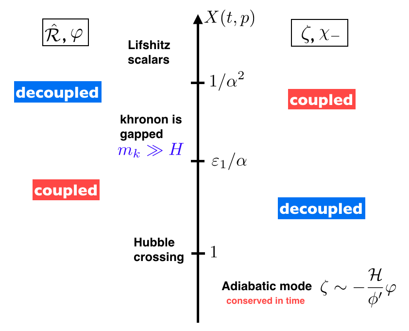
Figure 1: Summary of the time evolution of the fluctuations. The central axis denotes the quantity $X(t,p)$ introduced in Eq. (64).

3.2.3 Long wavelength evolution and power spectrum

We have shown that the variables $\chi_{\pm}$ are independent as long as the frequencies of the modes remain higher than the Hubble rate. As the modes redshift and approach the ‘horizon crossing’, $X\simeq 1$, the situation gets more complicated due to the terms proportional to ${\cal H}$ in the Lagrangian that can no longer be neglected. However, the situation simplifies again for ‘super Hubble’ modes corresponding to the regime:

(d) $X\ll 1$. In the standard relativistic single field inflation the curvature perturbation $\zeta$ is conserved at these scales. In Appendix A we show that this also holds for non-projectable HL gravity, despite the presence of khronon, by explicitly writing the quadratic Lagrangian in terms of $\zeta$ and $\varphi$. All non-derivative terms in the $\zeta$-equation turn out to be suppressed by $X$, so that we obtain the solution,

$$\zeta=const\;.$$ (87)

This allows to immediately write down the power spectrum for $\zeta$ by matching to the amplitude of $\chi_{+}$ fluctuations at the Hubble crossing, see Eq. (85),

$${\cal P}_{\zeta}(p)=\frac{1}{2\varepsilon_{1,p}M_{P}^{2}}\,{\cal P}_{LS}(p)\,,$$ (88)

where ${\cal P}_{LS}(p)$ is the power spectrum of the Lifshitz scalar and $\varepsilon_{1,p}$ is the value of the slow-roll parameter at the Hubble crossing time of the mode $p$. Explicitly we have,

$${\cal P}_{\zeta}(p)=\frac{\alpha_{1}^{\nu(z-1)}}{\varepsilon_{1,p}\varkappa_{z}^{\nu}}\frac{(2^{\nu}\Gamma[\nu])^{2}}{16\pi^{3}}z^{\frac{3}{z}-1}\left(\frac{H_{p}}{M_{P}}\right)^{\frac{3}{z}-1}\,,\qquad\qquad\nu=\frac{3}{2z}\;.$$ (89)

Note that for $z=3$ the spectrum is independent of the Hubble rate at inflation,

$${\cal P}_{\zeta}(p)=\frac{1}{8\pi^{2}}\frac{\alpha_{1}}{\varepsilon_{1,p}\sqrt{\varkappa_{3}}}\;,\qquad\qquad z=3\;.$$ (90)

The spectral index is given by

$$n_{s}-1\equiv\frac{{\rm d}\mathop{\rm ln}\nolimits{\cal{P}}_{\zeta}}{{\rm d}\mathop{\rm ln}\nolimits p}=-\frac{3-z}{z}\varepsilon_{1}-\varepsilon_{2}\,,$$ (91)

or alternatively,

$$n_{s}-1=-\frac{3(1+z)}{z}\varepsilon_{V}+2\eta_{V}\,.$$ (92)

For $z=1$ we recover the standard expressions.

We now analyze the super Hubble behavior of khronon, or ‘isocurvature’ mode. Despite the fact that the frequency term for $\varphi$ in the Lagrangian (119), as well as its mixing with $\zeta$, are suppressed by $X$, it still evolves non-trivially, because its time derivative term is also proportional to $X$. When the contributions with Lifshitz scaling $z=2,3$ dominate, the equation for $\varphi$ following from (119), (121) simplifies,

$$\varphi^{\prime\prime}-2{\cal H}(z-1)\varphi^{\prime}+a^{2}m_{k,z}^{2}\big{(}\varphi+\sqrt{2\varepsilon_{1}}M_{P}\zeta)=0\;.$$ (93)

The combination in brackets in the last term is nothing but $\sqrt{2\varepsilon_{1}}M_{P}{\cal R}$, which also coincides with $\chi_{-}$, up to slow-roll suppressed corrections. Also Eq. (93) is the same as the khronon equation (76). We conclude that khronon preserves its identity through Hubble crossing. Despite very long wavelength of the modes, they continue to rapidly oscillate with growing amplitude due to anti-friction. The decoupling of $\zeta$ and ${\cal R}$ now receives an intuitive explanation: these excitations have very different frequencies and therefore cannot mix.

The amplitude of khronon oscillations seizes to grow when the momentum redshifts down to $p/aM_{*}\simeq 1$. For $\sqrt{\varepsilon_{1}}\ll p/aM_{*}\ll 1$ the equation for $\varphi$ reads,

$$\varphi^{\prime\prime}+\beta_{4}\frac{p^{2}m_{k,2}^{2}}{M_{*}^{2}}\big{(}\varphi+\sqrt{2\varepsilon_{1}}M_{P}\zeta)=0\;,$$ (94)

and describes pure oscillations of ${\cal R}$ with constant amplitude. This is illustrated in Fig. 2. Finally, for $p/aM_{*}\ll\sqrt{\varepsilon_{1}}$ the $\varphi$-equation becomes,

$$\varphi^{\prime\prime}+\frac{2{\cal H}^{2}\varepsilon_{1}}{\alpha_{1}}\Big{(}\varkappa_{1}-\frac{\alpha_{1}}{\alpha_{3}}\Big{)}\varphi=0\;.$$ (95)

First, we notice that $\varphi$ has completely decoupled from $\zeta$. This is consistent with the result of [18] which studied inflation in the $z=1$ limit of HL gravity and identified the independent modes in the super Hubble regime as $\zeta$ and $\delta{\cal N}=({\cal H}/\phi^{\prime})\varphi$. The latter has geometric interpretation of the difference in the number of $e$-foldings between the surfaces of constant inflaton (i.e. constant density) and constant khronon. Second, the nature of solutions to (95) depends on the sign of the combination in brackets which has the physical meaning of the difference between (the squares of) the low-energy velocities of the inflaton, $c_{\varphi}^{2}\equiv\varkappa_{1}$, and graviton $c_{\gamma}^{2}\equiv\alpha_{1}/\alpha_{3}$ (see Eqs. (14), (31)). If it is positive, the mode $\varphi$ performs rapid oscillations with the physical frequency $\omega_{\varphi}/a\simeq H\sqrt{\varepsilon_{1}/\alpha_{1}}\gg H$ and the amplitude decaying as $a^{-1/2}$. On the other hand, if $\varkappa_{1}<\alpha_{1}/\alpha_{3}$, the solutions to (95) exhibit an exponential runaway behavior, signaling an instability. These two cases are illustrated in Fig. 2. To avoid instability, we will assume that $\varkappa_{1}>\alpha_{1}/\alpha_{3}$.

Equation (95) has been derived under the assumption that the low-energy velocities of inflaton and graviton differ by a factor of order one. Alternatively, one can impose the requirement that this difference should be small, $c_{\varphi}^{2}-c_{\gamma}^{2}={\cal O}(\alpha)$, which corresponds to an emergence of approximate Lorentz invariance at low energies. In this case one must retain additional contributions of the same order in the expression (LABEL:tomegaphi) for the frequency of $\varphi$, so that the $\varphi$-Lagrangian becomes,

$$\tilde{\cal L}_{\varphi}=a^{2}\frac{\alpha_{1}}{4\varepsilon_{1}}\bigg{(}\frac{p}{\cal H}\bigg{)}^{2}\bigg{[}{\varphi^{\prime}}^{2}-{\cal H}^{2}\,\varepsilon_{1}\bigg{(}1-\frac{\varepsilon_{2}}{2\varepsilon_{1}}+\frac{2(c^{2}_{\varphi}-c^{2}_{\gamma})}{\alpha_{1}}+\frac{3c_{k}^{2}}{c_{\gamma}^{2}}\bigg{)}\,\varphi^{2}\bigg{]}\;,$$ (96)

where $c_{k}^{2}\equiv 2\alpha_{1}\bar{\alpha}/\alpha_{3}^{2}$ is the low-energy velocity of the khronon. Upon proper translation of notations, this coincides with the Lagrangian for the isocurvature mode obtained in [18]. From (96) we see that the isocurvature mode evolves slowly with the rate suppressed by the slow-roll parameter $\varepsilon_{1}$. This behavior is also illustrated in Fig. 2.

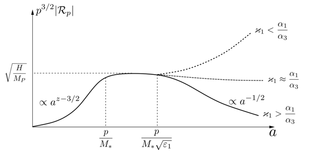
Figure 2: The amplitude of a khronon mode with conformal momentum $p$ as a function of the scale factor. It grows in the Lifshitz regime and reaches the value $\sqrt{H/M_{P}}$. Then it remains constant till $a\sim p/M_{*}\sqrt{\varepsilon_{1}}$, where the mode enters into the $z=1$ scaling. The subsequent evolution depends on the relation between velocities of the inflaton and graviton characterized by the parameters $\varkappa_{1}$ and $\alpha_{1}/\alpha_{3}$, as explained in the main text.

Even if the isocurvature mode does not develop instability at late times, it initially grows due to anti-friction, see Eq. (93) and Fig. 2. By the time the growth terminates the power spectrum of ${\cal R}$ reaches

$${\cal P}_{\cal R}\Big{|}_{a=p/M_{*}}=\frac{H^{2}}{4\pi^{2}m_{k,z}M_{*}}\simeq\frac{H}{4\pi^{2}M_{P}}\;.$$ (97)

For the validity of the linearized theory developed above we must require that the perturbations of ${\cal R}$ do not exceed unity. Then we obtain an upper bound on the inflationary Hubble scale,

$$H<4\pi^{2}M_{P}\;.$$ (98)

This constraint is somewhat unexpected, as a priori HL gravity should be applicable also at trans-Planckian energies. In fact, the requirement (98) may be too restrictive. It follows from consideration of metric perturbations with very long wavelengths. Unlike in GR, we cannot use a space-dependent reparameterization of time to remove this perturbation completely. However, space-independent time reparameterizations are still a symmetry of HL gravity and can be used to remove the fluctuation ${\cal R}$ at any given point. This suggests that coupling of khronon to other physical degrees of freedom should involve spatial derivatives and its almost homogeneous fluctuation, even with a large amplitude, should not have any effect locally. This property is indeed satisfied by the Lagrangian (121) describing dynamics of $\zeta$ and khronon at super Hubble scales. We have also verified that in pure de Sitter universe the growth of ${\cal R}$ does not lead to divergence of local gauge invariant observables constructed out of the metric $h_{ij}$, such as the extrinsic curvature $K$ and $K^{i}\!_{j}K^{j}\!_{i}$ and the spatial Ricci scalar $R$. For instance, the linear perturbation of the trace part of the extrinsic curvature is given by

$$\delta K=K-3H=-\frac{1-2\bar{\alpha}}{\bar{\alpha}}\left[(1-\Omega_{1})\dot{{\cal R}}-\Omega_{2}H{\cal R}\right]\propto a^{-(z+\frac{3}{2})}\,.$$ (99)

These arguments indicate that the constraint (98) may be avoided by a more careful treatment where the growth of super Hubble khronon fluctuations is absorbed by an appropriate field redefinition. This study is, however, beyond the scope of the present paper.

Before concluding this section, let us describe what happens if the slow-roll parameter $\varepsilon_{1}$ is the smallest quantity in the setup,

$$\varepsilon_{1}/\alpha_{1}\ll 1\;.$$ (100)

In this case the perturbations ${\cal R}$ and $\varphi$ are decoupled all the way through the Hubble crossing down to $X\simeq\varepsilon_{1}/\alpha$. After that, the good variables are $\zeta$ and $\varphi$. As before, $\zeta$ is conserved, whereas the evolution of $\varphi$ is described by Eqs. (93), (94), (95), (96). The power spectrum of $\zeta$ is determined by matching it to the fluctuations of the inflaton and khronon at $X\simeq\varepsilon_{1}/\alpha$. It is easy to see that the inflaton fluctuations dominate, so the spectrum is still given by (89) (leaving aside a small correction due to the damping of the inflaton perturbations between the Hubble crossing and $X\simeq\varepsilon_{1}/\alpha$). Note that for $z=3$ the hierarchy (100) is actually not viable, as it would imply that the power spectrum is larger than unity, see Eq. (90).

4 Violation of consistency relation

In the previous section, we computed the power spectra of the adiabatic curvature perturbation $\zeta$ and the primordial gravitational waves in the anisotropic scaling regime of HL gravity. In particular, we have shown that in the non-projectable case $\zeta$ is conserved at super Hubble scales during inflation, despite the presence of an isocurvature scalar perturbation. The intuitive explanation of this conservation is that the isocurvature mode, associated to the shift of khronon, is locally unobservable and its interaction with $\zeta$ is suppressed by spatial derivatives. This suggests that $\zeta$ will not be affected by the isocurvature mode at super Hubble scales also after the end of inflation. Indeed, conservation of $\zeta$ at super Hubble scales has been demonstrated for rather general matter content in the low-energy limit ($z=1$) of non-projectable HL gravity in Refs. [18, 31]. We will proceed under the assumption that this also holds between the end of inflation and the time when the universe enters into the isotropic scaling regime. Below we discuss a signal of the Lifshitz scaling in the primordial spectra.

4.1 Consistency relation in 4D Diff invariant theories

Before discussing the primordial spectra generated in the anisotropic scaling regime, let us review the discussion in theories encompassed by the Effective Field Theory (EFT) of inflation [46] where the inflaton background breaks 4D Diff invariance down to time-dependent spatial Diff. We follow Ref. [42]. Within EFT of inflation, the quadratic action for the gravitational waves is given by

$$S_{\gamma\gamma}=\frac{1}{8}\int{{\rm d}t\,{\rm d}^{3}\hbox{\boldmath{$x$}}\,a^{2}\,\frac{M^{2}_{P}}{c_{\gamma}^{2}}\left[(\gamma^{\prime}_{ij})^{2}-c^{2}_{\gamma}(\partial_{k}{\gamma_{ij}})^{2}\right]}\,.$$ (101)

In the presence of a time-dependent inflaton background which breaks Lorentz invariance and time-translations, the parameters $M_{P}$ and $c_{\gamma}$ can deviate from their vacuum values and can vary with time. However, one can always set these parameters to fixed values by a redefinition of the metric. Indeed, performing the disformal transformation:

$$g_{\mu\nu}\mapsto g_{\mu\nu}+(1-c^{2}_{\gamma}(t))n_{\mu}n_{\nu}\,,$$ (102)

where $n_{\mu}$ is the unit vector orthogonal to the constant-inflaton slices, and successively performing the conformal transformation to the Einstein frame,

$$g_{\mu\nu}\mapsto c^{-1}_{\gamma}(t)\frac{M_{P}^{2}(t)}{M^{2}_{P,0}}g_{\mu\nu}\,,$$ (103)

we can set the graviton speed $c_{\gamma}$ to unity and $M_{P}^{2}$ to constant. The equivalence between the Einstein frame and the Jordan frame for the gravitational waves was explicitly confirmed in Ref. [42]. The price to pay is that these transformations also alter the sector of scalar perturbations. For instance, if the propagation speed of the inflaton $c_{s}$ is 1 in the original frame, after the above disformal transformation which sets $c_{\gamma}$ to 1, the sound speed $c_{s}$ is changed into $c_{s}=c^{-1}_{\gamma}$.

After inflation, the non-minimal coupling introduced by the inflaton should disappear. Therefore, it is reasonable to calculate the primordial spectra in the Einstein frame for the gravitational waves. Then the spectrum for the gravitational waves is given by the standard expression and depends only on the ratio of inflationary Hubble scale and Planck mass. Besides, one obtains the well-known consistency relation

$$n_{t}=-\frac{r}{8c_{s}}\,,$$ (104)

which relates the spectral index for the gravitational waves $n_{t}$ and the tensor to scalar ratio $r$. (The sub leading contribution to the consistency relation in the slow-roll approximation can be found, e.g., in Ref. [47].) In a Lorentz invariant theory the velocity of any excitation cannot exceed unity, $c_{s}\leq 1$, which implies a bound,

$$-n_{t}\geq\frac{r}{8}\,.$$ (105)

This is a robust prediction of (single field) EFT of inflation. Moreover, when $c_{s}$ is smaller than $1$ the equilateral non-Gaussianity is enhanced by $1/c_{s}^{2}$ (see, e.g., Refs. [48, 49, 50]). Thus, a deviation from equality in (105) should be accompanied by large non-Gaussianity.

4.2 Violation of consistency relation in Hořava–Lifshitz gravity

We now discuss the primordial spectra generated in gravity with anisotropic scaling. In this case the symmetry breaking pattern is different: there are no 4D Diff to start with, but only the reduced symmetry of foliation-preserving Diff, that is further broken to time-dependent spatial Diff by the inflaton background. The velocity of graviton depends now on the wavenumber $p$, so one cannot set it to unity by the disformal transformation which globally changes the time component of the metric. This means that the modified dispersion relation physically changes the spectrum of the gravitational waves. In particular, the relation between the power spectrum ${\cal P}_{\gamma}$, Eq. (47), and the inflationary Hubble rate is no longer straightforward: it depends on the scaling exponent $z$ and other parameters of the theory. For $z=3$ the tensor power spectrum does not depend on $H$ at all. On the other hand, a robust prediction for $z=3$ is vanishing of the tensor spectral index, $n_{t}=0$.

Using Eqs. (47) and (89), at the leading order in the slow-roll approximation, we obtain the tensor-to-scalar ratio as

$$r\equiv\frac{{\cal P}_{\gamma}}{{\cal P}_{\zeta}}\simeq 16\varepsilon_{1}\left(\frac{\varkappa_{z}}{\varkappa_{\gamma,z}}\right)^{\frac{3}{2z}}\,.$$ (108)

Exceptionally, for $\varkappa_{z}=\varkappa_{\gamma,z}$ the tensor-to-scalar ratio is given by the standard expression irrespective of the value of $z$. Using Eqs. (48) and (108), we obtain the modified consistency relation for the primordial perturbations in the anisotropic scaling regime as

$$n_{t}\simeq-\frac{3-z}{z}\frac{r}{16}\left(\frac{\varkappa_{\gamma,z}}{\varkappa_{z}}\right)^{\frac{3}{2z}}\,.$$ (109)

We see that $n_{t}$ and $r$ are still related linearly, but the coefficient depends on $z$, $\varkappa_{z}$, and $\varkappa_{\gamma,z}$. Clearly, this can violate the lower bound (105) on $-n_{t}$ obtained in Lorentz invariant theories.

5 Concluding remarks

HL gravity contains an additional scalar degree of freedom in the gravity sector, khronon, corresponding to fluctuations of the preferred time foliation. Therefore, a minimal model of inflation possesses two scalar degrees of freedom: the inflaton and khronon. These two fields are coupled gravitationally. In the small scale limit, as usual, the gravitational interaction is suppressed and we simply have two decoupled Lifshitz scalar fields. Naively, one may expect that in the large scale limit, the gravitational interaction becomes important and these two fields start to be coupled. This is indeed the case in the projectable version of HL gravity. The inflaton and khronon stay nearly gapless modes which are bi-linearly coupled. Then the adiabatic curvature perturbation $\zeta$ is generically not conserved at large scales.

On the other hand, the situation is crucially different in the non-projectable version. In the anisotropic scaling regime, khronon acquires the effective mass $m_{K}$, which is much larger than the Hubble scale, well before Hubble crossing time. It then decouples from the adiabatic mode $\zeta$ and does not leave any impact on the power spectrum of $\zeta$, which is conserved at super Hubble scales. The power spectrum of $\zeta$ is simply given by that of the Lifshitz scalar with the multiplicative factor $1/(2\varepsilon_{1}M_{P}^{2})$. The decoupled khronon rapidly oscillates, with the amplitude of the oscillations growing exponentially due to anti-friction. The growth persists until the mode enters into the regime of isotropic scaling as a consequence of the redshift of its momentum. We need a more careful consideration to see if this exponential growth can or cannot affect observable quantities.

One remaining question is whether the decoupling between the adiabatic mode $\zeta$ and khronon is a robust feature of non-projectable HL gravity also beyond the restricted setup considered in this paper. We have focused on the linear order in perturbations. The physical interpretation presented in Sec. 3.2 suggests that the decoupling will also persist at non-linear orders. We postpone an explicit analysis of this issue, as well as of primordial non-Gaussianity, to a future work. In this paper we assumed the minimal coupling of the inflaton to the gravity sector. One may wonder whether a non-minimal interaction can prevent the decoupling of khronon. Recall that khronon gets gapped due to a peculiar structure of the coefficient in front of the (quadratic) time derivative term in the action. Thus, to make khronon gapless, the non-minimal coupling should modify the time derivative terms. The only contribution that can change the time derivative terms under the assumption of foliation-preserving Diff and time reversal symmetry is the term with $K\dot{\Phi}/N$. However, this can be removed by a redefinition of the metric $h_{ij}\to\Omega^{2}(\Phi)h_{ij}$ and $N\to\Omega^{3}(\Phi)N$. Therefore, we expect that the decoupling between $\zeta$ and khronon takes place generically in the non-projectable version of HL gravity with the time reversal symmetry in the anisotropic scaling regime. It may be interesting to study if this decoupling takes place also in the case when the time reversal symmetry is broken, e.g. by a term with $\sqrt{h}\,\dot{\Phi}/N$.

We also pointed out that the consistency relation between the tensor to scalar ratio $r$ and the tensor spectral index $n_{t}$, which holds in the general single field EFT of inflation, can be violated by the primordial perturbations generated during the anisotropic scaling regime. If the primordial gravitational waves are detected, the value of $r$ will give the lower bound on $-n_{t}$ in Lorentz invariant theory. A violation of this bound will indicate violation of Lorenz invariance in the early universe.

Appendix A Quadratic action

In this Appendix we give the complete expression of the quadratic action for the mixed system of the inflaton and khronon.

A.1 Action for ${\cal R}$ and $\varphi$

Substituting the fields (49) into the Lagrangian consisting of (3) and (10), expanding to second order in perturbations and integrating out the lapse function and the shift vector, we obtain

$$S=\int{\rm d}^{4}x{\cal L}=\int{\rm d}t\int{\rm d}^{3}\hbox{\boldmath{$p$}}\left[{\cal L}_{{\cal R}}+{\cal L}_{\varphi}+{\cal L}_{{\cal R}\varphi}\right]$$ (110)

with

$${\cal L}_{{\cal R}}=a^{2}M_{*}^{2}\frac{1+\bar{\alpha}}{\alpha_{1}\bar{\alpha}}\left[(1-\Omega_{1}(t,\,p)){\cal R}^{\prime}_{\hbox{\boldmath{\scriptsize$p$}}}{\cal R}^{\prime}_{-\hbox{\boldmath{\scriptsize$p$}}}-\omega_{{\cal R}}^{2}(t,\,p){\cal R}_{\hbox{\boldmath{\scriptsize$p$}}}{\cal R}_{-\hbox{\boldmath{\scriptsize$p$}}}\right]\,,$$ (111)

$${\cal L}_{\varphi}=\frac{a^{2}}{2}\left[\left(1-\frac{\bar{\alpha}\varepsilon_{1}}{1-2\bar{\alpha}}\Omega_{1}(t,\,p)\right)\varphi^{\prime}_{\hbox{\boldmath{\scriptsize$p$}}}\varphi^{\prime}_{-\hbox{\boldmath{\scriptsize$p$}}}-\omega^{2}_{\varphi}(\eta,\,p)\varphi_{\hbox{\boldmath{\scriptsize$p$}}}\varphi_{-\hbox{\boldmath{\scriptsize$p$}}}\right]\,,$$ (112)

$${\cal L}_{{\cal R}\varphi}=a^{2}\bigg{\{}-\frac{\phi^{\prime}}{\cal H}\Omega_{1}(t,\,p)\varphi^{\prime}_{\hbox{\boldmath{\scriptsize$p$}}}{\cal R}^{\prime}_{-\hbox{\boldmath{\scriptsize$p$}}}+\left[\frac{1-2\bar{\alpha}}{\bar{\alpha}}(1-\Omega_{1}(t,\,p))\phi^{\prime}+\Omega_{1}(t,\,p)\frac{\phi^{\prime\prime}-{\cal H}\phi^{\prime}}{{\cal H}}\right]\varphi_{\hbox{\boldmath{\scriptsize$p$}}}{\cal R}^{\prime}_{-\hbox{\boldmath{\scriptsize$p$}}}$$

$$\qquad\qquad\qquad\qquad-\phi^{\prime}\Omega_{2}(t,\,p)\varphi^{\prime}_{\hbox{\boldmath{\scriptsize$p$}}}{\cal R}_{-\hbox{\boldmath{\scriptsize$p$}}}-\left(\frac{1+\bar{\alpha}}{\bar{\alpha}}{\cal H}\phi^{\prime}+a^{2}V_{\phi}\right)\Omega_{2}(t,\,p)\varphi_{\hbox{\boldmath{\scriptsize$p$}}}{\cal R}_{-\hbox{\boldmath{\scriptsize$p$}}}\bigg{\}}\,,$$ (113)

where the functions $\Omega_{1,2}(t,p)$ have been introduced in (60), (61), the frequency $\omega_{{\cal R}}$ is given by Eq. (63) and $\omega_{\varphi}$ is given by

$$\frac{\omega^{2}_{\varphi}(t,\,p)}{{\cal H}^{2}}=\biggl{(}\frac{p}{{\cal H}}\biggr{)}^{2}\left[\varkappa_{1}+\varkappa_{2}\biggl{(}\frac{p}{aM_{*}}\biggr{)}^{2}+\varkappa_{3}\biggl{(}\frac{p}{aM_{*}}\biggr{)}^{4}\right]+\frac{a^{2}V_{\phi\phi}}{{\cal H}^{2}}-\frac{1+\bar{\alpha}}{\bar{\alpha}}\varepsilon_{1}$$ (114)

$$\qquad\qquad\qquad\qquad\quad+\frac{(1+\bar{\alpha})\alpha_{1}}{2\bar{\alpha}M_{*}^{2}}\biggl{(}\phi^{\prime}+\frac{\bar{\alpha}}{1+\bar{\alpha}}\frac{a^{2}V_{\phi}}{\cal H}\biggr{)}^{\!2}\frac{\Omega_{1}(t,\,p)}{{\cal H}^{2}}$$ (115)

$$\qquad\qquad\qquad\qquad\quad-\frac{\alpha_{1}}{2M_{*}^{2}}\frac{1}{({\cal H}a)^{2}}\biggl{[}a^{2}\phi^{\prime}\bigg{(}\phi^{\prime}+\frac{\bar{\alpha}}{1+\bar{\alpha}}\frac{a^{2}V_{\phi}}{\cal H}\bigg{)}\frac{\Omega_{1}(t,\,p)}{\cal H}\!\biggr{]}^{\prime}.$$ (116)

By inspection of various terms in the Lagrangian we can see that ${\cal R}$ and $\varphi$ are decoupled in the limit of large momenta $p$.

A.2 Action for $\zeta$ and $\varphi$

Using $\zeta$ defined in (85) and eliminating ${\cal R}$, we obtain the quadratic action as

$$S=\int{\rm d}t\int{\rm d}^{3}\hbox{\boldmath{$p$}}\left[{\cal L}_{\zeta}+\tilde{{\cal L}}_{\varphi}+{\cal L}_{\zeta\varphi}\right]$$ (117)

with

$${\cal L}_{\zeta}=a^{2}M_{*}^{2}\frac{1+\bar{\alpha}}{\alpha_{1}\bar{\alpha}}\left[(1-\Omega_{1}(t,\,p))\zeta^{\prime}_{\hbox{\boldmath{\scriptsize$p$}}}\zeta^{\prime}_{-\hbox{\boldmath{\scriptsize$p$}}}-\omega_{{\cal R}}^{2}(t,\,p)\zeta_{\hbox{\boldmath{\scriptsize$p$}}}\zeta_{-\hbox{\boldmath{\scriptsize$p$}}}\right]\,,$$ (118)

$$\tilde{\cal L}_{\varphi}=\frac{a^{2}}{2}\left[\frac{(1-2\bar{\alpha})\alpha_{1}}{2(1+\bar{\alpha})\varepsilon_{1}}\left(1+\frac{\bar{\alpha}\varepsilon_{1}}{1-2\bar{\alpha}}\right)\Omega_{3}(t,\,p)\varphi^{\prime}_{\hbox{\boldmath{\scriptsize$p$}}}\varphi^{\prime}_{-\hbox{\boldmath{\scriptsize$p$}}}-\tilde{\omega}^{2}_{\varphi}(t,\,p)\varphi_{\hbox{\boldmath{\scriptsize$p$}}}\varphi_{-\hbox{\boldmath{\scriptsize$p$}}}\right]\,,$$ (119)

$${\cal L}_{\zeta\varphi}=a^{2}\bigg{\{}M_{*}^{2}\frac{{\cal H}}{\phi^{\prime}}\Omega_{3}(t,\,p)\left(\zeta^{\prime}_{\hbox{\boldmath{\scriptsize$p$}}}\varphi^{\prime}_{-\hbox{\boldmath{\scriptsize$p$}}}-\frac{\phi^{\prime\prime}-{\cal H}\phi^{\prime}}{\phi^{\prime}}\zeta^{\prime}_{\hbox{\boldmath{\scriptsize$p$}}}\varphi_{-\hbox{\boldmath{\scriptsize$p$}}}\right)-\phi^{\prime}\Omega_{2}(t,\,p)\zeta_{\hbox{\boldmath{\scriptsize$p$}}}\varphi^{\prime}_{-\hbox{\boldmath{\scriptsize$p$}}}$$ (120)

$$\quad\qquad\quad\quad-\left[2M_{*}^{2}\frac{1+\bar{\alpha}}{\alpha_{1}\bar{\alpha}}\frac{{\cal H}}{\phi^{\prime}}\omega^{2}_{{\cal R}}(t,\,p)+\!\left(\frac{1+\bar{\alpha}}{\bar{\alpha}}{\cal H}\phi^{\prime}+a^{2}V_{\phi}\right)\Omega_{2}(t,\,p)\right]\!\zeta_{\hbox{\boldmath{\scriptsize$p$}}}\varphi_{-\hbox{\boldmath{\scriptsize$p$}}}\bigg{\}}\,,$$ (121)

where we introduced

$$\Omega_{3}(t,\,p)=\biggl{(}\frac{p}{{\cal H}}\biggr{)}^{2}\biggl{[}1+\frac{1}{\beta_{4}}\biggl{(}\frac{p}{aM_{*}}\biggr{)}^{2}+\frac{1}{\gamma_{4}}\biggl{(}\frac{p}{aM_{*}}\biggr{)}^{4}\biggr{]}\Omega_{1}(t,\,p)\,.$$ (122)

The new expression for the $\varphi$-frequency is

$$\frac{\tilde{\omega}_{\varphi}^{2}(t,\,p)}{{\cal H}^{2}}=\biggl{(}\frac{p}{{\cal H}}\biggr{)}^{2}\left[\varkappa_{1}+\varkappa_{2}\biggl{(}\frac{p}{aM_{*}}\biggr{)}^{2}+\varkappa_{3}\biggl{(}\frac{p}{aM_{*}}\biggr{)}^{4}\right]+\frac{1-2\bar{\alpha}}{\varepsilon_{1}\bar{\alpha}}\frac{\omega_{{\cal R}}^{2}(t,\,p)}{{\cal H}^{2}}$$ (123)

$$\qquad\qquad\quad-\frac{\alpha_{1}\bar{\alpha}}{2(1+\bar{\alpha})}\left\{\frac{1-2\bar{\alpha}}{\bar{\alpha}}\varepsilon_{1}+\left(\varepsilon_{1}-\frac{\varepsilon_{2}}{2}\right)^{2}\right\}\Omega_{3}(t,\,p)$$ (124)

$$\qquad\qquad\quad+\frac{1}{(a{\cal H})^{2}}\left\{a^{2}{\cal H}\left[-\Omega_{2}(t,\,p)+\frac{(1-2\bar{\alpha})\alpha_{1}}{2(1+\bar{\alpha})\varepsilon_{1}}\left(\varepsilon_{1}-\frac{\varepsilon_{2}}{2}\right)\bigg{(}1+\frac{\varepsilon_{1}\bar{\alpha}}{1-2\bar{\alpha}}\bigg{)}\Omega_{3}(t,\,p)\right]\right\}^{\prime}$$ (125)

$$\qquad\qquad\quad+2\left(\frac{1-2\bar{\alpha}}{\bar{\alpha}}+\varepsilon_{1}-\frac{\varepsilon_{2}}{2}\right)\Omega_{2}(t,\,p)-\frac{(1-2\bar{\alpha})\alpha_{1}}{8(1+\bar{\alpha})}\frac{\varepsilon_{2}}{\varepsilon_{1}}(\varepsilon_{2}-4\varepsilon_{1})\Omega_{3}(t,\,p).$$ (126)

Notice that all terms in ${\cal L}_{\zeta\varphi}$ and $\tilde{\cal L}_{\varphi}$ are multiplied by factors of order ${\cal O}(X)$. This implies that $\zeta$ has a constant solution in the long-wavelength limit. As discussed in the main text, the degree of freedom which is orthogonal to $\zeta$ acquires a mass gap which is much larger than $H$ in the anisotropic scaling regime.

Appendix B Khronon-inflaton mixing for $z=1$

If the inflationary Hubble rate is low, $H<M_{*}\sqrt{\alpha_{1}/\varepsilon_{1}}$, mixing between the inflaton and khronon perturbations occurs in the regime where the dynamics is dominated by the terms with relativistic scaling $z=1$. In this Appendix, we consider the case with $\varepsilon_{1}/\alpha>1$ and the range $X\ll 1/\alpha^{2}$.

Compared to the Lagrangian (78) considered in the main text, one should keep an additional mixing contribution, so that the total mixing Lagrangian reads,

$${\cal L}_{{\cal R}\varphi}=a^{2}\,\bigg{[}-\frac{\varphi_{\hbox{\boldmath{\scriptsize$p$}}}^{\prime}\hat{R}_{-\hbox{\boldmath{\scriptsize$p$}}}^{\prime}}{\sqrt{1+\frac{\alpha_{1}X}{2\varepsilon_{1}}}}+\frac{\alpha_{1}}{\alpha_{3}}\frac{{\cal H}^{2}X}{\sqrt{1+\frac{\alpha_{1}X}{2\varepsilon_{1}}}}\varphi_{\hbox{\boldmath{\scriptsize$p$}}}\hat{R}_{-\hbox{\boldmath{\scriptsize$p$}}}\bigg{]}\;.$$ (128)

The quantity $X$ is now given simply by,

$$X=(p/{\cal H})^{2}\;,$$

whereas the fields’ frequencies are,

$$\hat{\omega}_{\cal R}^{2}=p^{2}\frac{\alpha_{1}}{\alpha_{3}}\frac{1+\frac{\alpha_{1}\bar{\alpha}}{\alpha_{3}\varepsilon_{1}}X}{1+\frac{\alpha_{1}X}{2\varepsilon_{1}}}~{},~{}~{}~{}~{}~{}~{}\omega_{\varphi}^{2}=\varkappa_{1}p^{2}\;.$$

At $X\gg\varepsilon_{1}/\alpha_{1}$ the fields $\varphi$ and $\hat{\cal R}$ are decoupled and have the same velocities as the inflaton and khronon in flat spacetime, whereas at $X\ll\varepsilon_{1}/\alpha_{1}$ they become strongly mixed. To diagonalize the Lagrangian in the latter case, we write it in terms of $\varphi$ and

$$\chi_{+}=\varphi-\frac{\hat{\cal R}}{\sqrt{1+\frac{\alpha_{1}X}{2\varepsilon_{1}}}}\;.$$

It is straightforward to see that the mixing terms are negligible at $X\ll\varepsilon_{1}/\alpha_{1}$. Thus, we conclude that in this regime the decoupled modes are $\chi_{+}$ (or equivalently $\zeta$, see Eq. (85)) and $\varphi$. Their Lagrangian reads,

$${\cal L}=\frac{a^{2}}{2}\Big{(}{\chi_{+}^{\prime}}^{2}-\frac{\alpha_{1}}{\alpha_{3}}p^{2}\,\chi_{+}^{2}\Big{)}+\frac{a^{2}\alpha_{1}}{4\varepsilon_{1}}\bigg{(}\frac{p}{\cal H}\bigg{)}\bigg{[}\varphi^{\prime 2}-{\cal H}^{2}\frac{2\varepsilon_{1}}{\alpha_{1}}\Big{(}\varkappa_{1}-\frac{\alpha_{1}}{\alpha_{3}}\Big{)}\,\varphi^{2}\bigg{]}\;.$$ (129)

It is worth stressing that in this Appendix we have focused on ‘sub Hubble’ modes, i.e. modes with $X\gg 1$. Nevertheless, we observe that the $\varphi$-equation following from the Lagrangian (129) coincides with Eq. (95) obeyed by super Hubble isocurvature modes in the $z=1$ regime. In other words, in the $z=1$ case the adiabatic and isocurvature modes are described respectively by $\zeta$ and $\varphi$ at all times when $X\ll\varepsilon_{1}/\alpha_{1}$. Note that the velocity of the adiabatic mode is given by $\sqrt{\alpha_{1}/\alpha_{3}}$ and coincides with the velocity of gravitons, rather than the velocity of inflaton.

References

- [1] M. H. Goroff and A. Sagnotti, “The Ultraviolet Behavior of Einstein Gravity,” Nucl. Phys. B 266, 709 (1986).
- [2] K. S. Stelle, “Renormalization of higher-derivative quantum gravity”, Phys. Rev. D 16, 953 (1977).
- [3] P. Hořava, “Quantum Gravity at a Lifshitz Point,” Phys. Rev. D 79, 084008 (2009) [arXiv:0901.3775 [hep-th]].
- [4] A. O. Barvinsky, D. Blas, M. Herrero-Valea, S. M. Sibiryakov and C. F. Steinwachs, “Renormalization of Hořava gravity,” Phys. Rev. D 93, no. 6, 064022 (2016) [arXiv:1512.02250 [hep-th]].
- [5] A. O. Barvinsky, D. Blas, M. Herrero-Valea, S. M. Sibiryakov and C. F. Steinwachs, “Renormalization of gauge theories in the background-field approach,” arXiv:1705.03480 [hep-th].
- [6] A. O. Barvinsky, D. Blas, M. Herrero-Valea, S. M. Sibiryakov and C. F. Steinwachs, “Hořava gravity is asymptotically free (in 2+1 dimensions),” Phys. Rev. Lett. 119, no. 21, 211301 (2017) [arXiv:1706.06809 [hep-th]].
- [7] D. Mattingly, “Modern tests of Lorentz invariance,” Living Rev. Rel. 8, 5 (2005) [gr-qc/0502097].
- [8] V. A. Kostelecky and N. Russell, “Data Tables for Lorentz and CPT Violation,” Rev. Mod. Phys. 83, 11 (2011) [arXiv:0801.0287 [hep-ph]].
- [9] S. Liberati, “Tests of Lorentz invariance: a 2013 update,” Class. Quant. Grav. 30, 133001 (2013) [arXiv:1304.5795 [gr-qc]].
- [10] C. M. Will, “The Confrontation between general relativity and experiment,” Living Rev. Rel. 9, 3 (2006) [gr-qc/0510072].
- [11] K. Yagi, D. Blas, N. Yunes and E. Barausse, “Strong Binary Pulsar Constraints on Lorentz Violation in Gravity,” Phys. Rev. Lett. 112, no. 16, 161101 (2014) [arXiv:1307.6219 [gr-qc]].
- [12] K. Yagi, D. Blas, E. Barausse and N. Yunes, “Constraints on Einstein-aether theory and Hořava gravity from binary pulsar observations,” Phys. Rev. D 89, no. 8, 084067 (2014) Erratum: [Phys. Rev. D 90, no. 6, 069902 (2014)] [arXiv:1311.7144 [gr-qc]].
- [13] L. Shao, R. N. Caballero, M. Kramer, N. Wex, D. J. Champion and A. Jessner, “A new limit on local Lorentz invariance violation of gravity from solitary pulsars,” Class. Quant. Grav. 30, 165019 (2013) [arXiv:1307.2552 [gr-qc]].
- [14] J. Beltran Jimenez, F. Piazza and H. Velten, “Evading the Vainshtein Mechanism with Anomalous Gravitational Wave Speed: Constraints on Modified Gravity from Binary Pulsars,” Phys. Rev. Lett. 116, no. 6, 061101 (2016) [arXiv:1507.05047 [gr-qc]].
- [15] E. N. Saridakis, “Hořava-Lifshitz Dark Energy,” Eur. Phys. J. C 67, 229 (2010) [arXiv:0905.3532 [hep-th]].
- [16] S. Dutta and E. N. Saridakis, “Observational constraints on Hořava-Lifshitz cosmology,” JCAP 1001, 013 (2010) [arXiv:0911.1435 [hep-th]].
- [17] T. Kobayashi, Y. Urakawa and M. Yamaguchi, “Cosmological perturbations in a healthy extension of Hořava gravity,” JCAP 1004, 025 (2010) [arXiv:1002.3101 [hep-th]].
- [18] C. Armendariz-Picon, N. F. Sierra and J. Garriga, “Primordial Perturbations in Einstein-Aether and BPSH Theories,” JCAP 1007, 010 (2010) [arXiv:1003.1283 [astro-ph.CO]].
- [19] D. Blas, M. M. Ivanov and S. Sibiryakov, “Testing Lorentz invariance of dark matter,” JCAP 1210, 057 (2012) [arXiv:1209.0464 [astro-ph.CO]].
- [20] B. Audren, D. Blas, J. Lesgourgues and S. Sibiryakov, “Cosmological constraints on Lorentz violating dark energy,” JCAP 1308, 039 (2013) [arXiv:1305.0009 [astro-ph.CO]].
- [21] B. Audren, D. Blas, M. M. Ivanov, J. Lesgourgues and S. Sibiryakov, “Cosmological constraints on deviations from Lorentz invariance in gravity and dark matter,” JCAP 1503, no. 03, 016 (2015) [arXiv:1410.6514 [astro-ph.CO]].
- [22] D. Blas, M. M. Ivanov, I. Sawicki and S. Sibiryakov, “On constraining the speed of gravitational waves following GW150914,” Pisma Zh. Eksp. Teor. Fiz. 103 (2016) no.10, 708 [JETP Lett. 103 (2016) no.10, 624] [arXiv:1602.04188 [gr-qc]].
- [23] N. Yunes, K. Yagi and F. Pretorius, “Theoretical Physics Implications of the Binary Black-Hole Mergers GW150914 and GW151226,” Phys. Rev. D 94, no. 8, 084002 (2016) [arXiv:1603.08955 [gr-qc]].
- [24] B. P. Abbott et al. [LIGO Scientific and Virgo and Fermi-GBM and INTEGRAL Collaborations], “Gravitational Waves and Gamma-rays from a Binary Neutron Star Merger: GW170817 and GRB 170817A,” Astrophys. J. 848, no. 2, L13 (2017) [arXiv:1710.05834 [astro-ph.HE]].
- [25] A. Emir Gümrükçüoǧlu, M. Saravani and T. P. Sotiriou, “Hořava gravity after GW170817,” Phys. Rev. D 97, no. 2, 024032 (2018) [arXiv:1711.08845 [gr-qc]].
- [26] N. Arkani-Hamed, P. Creminelli, S. Mukohyama and M. Zaldarriaga, “Ghost inflation,” JCAP 0404, 001 (2004) [hep-th/0312100].
- [27] T. Takahashi and J. Soda, “Chiral Primordial Gravitational Waves from a Lifshitz Point,” Phys. Rev. Lett. 102, 231301 (2009) [arXiv:0904.0554 [hep-th]].
- [28] G. Calcagni, “Cosmology of the Lifshitz universe,” JHEP 0909, 112 (2009) [arXiv:0904.0829 [hep-th]].
- [29] E. Kiritsis and G. Kofinas, “Hořava-Lifshitz Cosmology,” Nucl. Phys. B 821, 467 (2009) [arXiv:0904.1334 [hep-th]].
- [30] S. Mukohyama, “Scale-invariant cosmological perturbations from Hořava-Lifshitz gravity without inflation,” JCAP 0906, 001 (2009) [arXiv:0904.2190 [hep-th]].
- [31] T. Kobayashi, Y. Urakawa and M. Yamaguchi, “Large scale evolution of the curvature perturbation in Hořava-Lifshitz cosmology,” JCAP 0911, 015 (2009) [arXiv:0908.1005 [astro-ph.CO]].
- [32] W. Donnelly and T. Jacobson, “Coupling the inflaton to an expanding aether,” Phys. Rev. D 82, 064032 (2010) [arXiv:1007.2594 [gr-qc]].
- [33] P. Creminelli, J. Norena, M. Pena and M. Simonovic, “Khronon inflation,” JCAP 1211, 032 (2012) [arXiv:1206.1083 [hep-th]].
- [34] A. R. Solomon and J. D. Barrow, “Inflationary Instabilities of Einstein-Aether Cosmology,” Phys. Rev. D 89, no. 2, 024001 (2014) [arXiv:1309.4778 [astro-ph.CO]].
- [35] M. M. Ivanov and S. Sibiryakov, “UV-extending Ghost Inflation,” JCAP 1405, 045 (2014) [arXiv:1402.4964 [astro-ph.CO]].
- [36] D. Wands, K. A. Malik, D. H. Lyth and A. R. Liddle, “A New approach to the evolution of cosmological perturbations on large scales,” Phys. Rev. D 62, 043527 (2000) [astro-ph/0003278].
- [37] S. Weinberg, “Adiabatic modes in cosmology,” Phys. Rev. D 67, 123504 (2003) [astro-ph/0302326].
- [38] D. Blas, O. Pujolas and S. Sibiryakov, “On the Extra Mode and Inconsistency of Horava Gravity,” JHEP 0910, 029 (2009) [arXiv:0906.3046 [hep-th]].
- [39] D. Blas, O. Pujolas and S. Sibiryakov, “Models of non-relativistic quantum gravity: The Good, the bad and the healthy,” JHEP 1104, 018 (2011) [arXiv:1007.3503 [hep-th]].
- [40] D. Blas, O. Pujolas and S. Sibiryakov, “Consistent Extension of Hořava Gravity,” Phys. Rev. Lett. 104, 181302 (2010) [arXiv:0909.3525 [hep-th]].
- [41] G. D. Moore and A. E. Nelson, “Lower bound on the propagation speed of gravity from gravitational Cherenkov radiation,” JHEP 0109, 023 (2001) [hep-ph/0106220].
- [42] P. Creminelli, J. Gleyzes, J. Norena and F. Vernizzi, “Resilience of the standard predictions for primordial tensor modes,” Phys. Rev. Lett. 113, no. 23, 231301 (2014) [arXiv:1407.8439 [astro-ph.CO]].
- [43] S. Mukohyama, “Hořava-Lifshitz Cosmology: A Review,” Class. Quant. Grav. 27, 223101 (2010) [arXiv:1007.5199 [hep-th]].
- [44] C. Gordon, D. Wands, B. A. Bassett and R. Maartens, “Adiabatic and entropy perturbations from inflation,” Phys. Rev. D 63, 023506 (2001) [astro-ph/0009131].
- [45] T. Jacobson, “Extended Hořava gravity and Einstein-aether theory,” Phys. Rev. D 81, 101502 (2010) Erratum: [Phys. Rev. D 82, 129901 (2010)] [arXiv:1001.4823 [hep-th]].
- [46] C. Cheung, P. Creminelli, A. L. Fitzpatrick, J. Kaplan and L. Senatore, “The Effective Field Theory of Inflation,” JHEP 0803, 014 (2008) [arXiv:0709.0293 [hep-th]].
- [47] D. Baumann, D. Green and R. A. Porto, “B-modes and the Nature of Inflation,” JCAP 1501, no. 01, 016 (2015) [arXiv:1407.2621 [hep-th]].
- [48] D. Seery and J. E. Lidsey, “Primordial non-Gaussianities in single field inflation,” JCAP 0506, 003 (2005) [astro-ph/0503692].
- [49] D. Baumann and D. Green, “Equilateral Non-Gaussianity and New Physics on the Horizon,” JCAP 1109, 014 (2011) [arXiv:1102.5343 [hep-th]].
- [50] P. A. R. Ade et al. [Planck Collaboration], “Planck 2015 results. XVII. Constraints on primordial non-Gaussianity,” Astron. Astrophys. 594, A17 (2016) [arXiv:1502.01592 [astro-ph.CO]].