A high-order discontinuous Galerkin approach to the elasto-acoustic problem

Abstract

We address the spatial discretization of an evolution problem arising from the coupling of viscoelastic and acoustic wave propagation phenomena by employing a discontinuous Galerkin scheme on polygonal and polyhedral meshes. The coupled nature of the problem is ascribed to suitable transmission conditions imposed at the interface between the solid (elastic) and fluid (acoustic) domains. We state and prove a well-posedness result for the strong formulation of the problem, present a stability analysis for the semi-discrete formulation, and finally prove an a priori $hp$-version error estimate for the resulting formulation in a suitable (mesh-dependent) energy norm. We also discuss the time integration scheme employed to obtain the fully discrete system. The convergence results are validated by numerical experiments carried out in a two-dimensional setting.

Introduction

This work is devoted to the development and analysis of a discontinuous Galerkin (dG) method on polygonal and polyhedral grids [1, 2, 3, 4] for an evolution problem modeling the coupling of viscoelastic and acoustic wave propagation phenomena. Such kind of problems arise, for example, in geophysics, namely in the modeling and simulation of seismic events near coastal environments. Other contexts in which this problem plays a major role are the modeling of sensing or actuation devices immersed in an acoustic fluid [5], as well as medical ultrasonics [6]. In practical applications, the underlying geometry one has to deal with is remarkably complicated and irregular; considering a conforming triangulation would therefore be computationally very expensive. We are thus led to consider a space discretization method capable to reproduce the geometrical constraints under consideration to a reasonable extent of accuracy, without being at the same time too much demanding. Such a discretization is then performed using general polygonal or polyhedral (briefly, polytopic) elements, with no restriction on the number of faces each element can possess, and possibly allowing for face degeneration in mesh refinement. The dG method has been recently proven to successfully support polytopic meshes: we refer the reader, e.g., to [7, 8, 9, 10, 11, 12, 13, 14, 15], as well as to the comprehensive research monograph by Cangiani et al. [16]. In addition to the dG method, several other methods are capable to support polytopic meshes, such as the Polygonal Finite Element method [17, 18, 19, 20], the Mimetic Finite Difference method [21, 22, 23, 24], the Virtual Element method [25, 26, 27, 28], the Hybridizable Discontinuous Galerkin method [29, 30, 31, 32, 33], and the Hybrid High-Order method [34, 35, 36, 37, 38].

An elasto-acoustic coupling typically occurs in the following framework: a domain made up by two subdomains, one occupied by a solid (elastic) body, the other by a fluid (acoustic) one, with suitable transmission conditions imposed at the interface between the two. The aim of such conditions is to account for the following physical properties:  (i) the normal component of the velocity field is continuous at the interface; (ii) a pressure load is exerted by the fluid body on the solid one through the interface. In this paper, the unknowns of the problem are the displacement field in the solid domain and the acoustic potential in the fluid domain; the latter, say $\varphi$, is defined in terms of the acoustic velocity field $\mathbf{v}_{a}$ in such a way that $\mathbf{v}_{a}=-\mathbf{\nabla}\varphi$. However, other formulations are possible; for instance, one can consider a pressure-based formulation in the acoustic subdomain [6], or a displacement-based formulation in both subdomains [39].

In a geophysics context, when a seismic event occurs, both pressure (P) and shear (S) waves are generated. However, only P-waves (i.e., whose direction of propagation is aligned with the displacement of the medium) are able to travel through both solid and fluid bodies, unlike S-waves (i.e., whose direction of propagation is orthogonal to the displacement of the medium), which can travel only through solids. This explains the reason for considering the first interface condition. On the other hand, the second one accounts for the fact that an acoustic wave propagating in a fluid domain of density $\rho_{a}$ gives rise to an acoustic pressure field of magnitude $\rho_{a}|\accentset{\mbox{\footnotesize.}}{\varphi}|$, $\accentset{\mbox{\footnotesize.}}{\varphi}$ denoting the first time derivative of the acoustic potential.

Mathematical and numerical aspects of the elasto-acoustic coupling have been the subject of an extremely broad literature. We give hereinafter a brief overview of some of the research works carried out so far in this field.

Barucq et al. [40] have characterized the Fréchet differentiability of the elasto-acoustic field with respect to Lipschitz-continuous deformation of the shape of an elastic scatterer. The same authors [41] have also proposed a dG method for computing the scattered field from an elastic bounded object immersed in an infinite homogeneous fluid medium, employing high-order polynomial-shape functions to address the high-frequency propagation regime, and curved boundary edges to provide an accurate representation of the fluid-structure interface. Bermúdez et al. [39] have solved an interior elasto-acoustic problem in a three-dimensional setting, employing a displacement-based formulation on both the fluid and the solid domains, and a discretization consisting of linear tetrahedral finite elements for the solid and Raviart–Thomas elements of lowest order for the fluid; a further unknown is introduced on the interface between solid and fluid to impose the trasmission conditions. Brunner et al. [42] have treated the case of thin structures and dense fluids; the structural part is modeled with the finite element method, and the exterior acoustic problem is efficiently modeled with the Galerkin boundary element method. De Basabe and Sen [43] have compared Finite Difference and Spectral Element methods for elastic wave propagation in media with a fluid-solid interface. Fischer and Gaul [44] have proposed a coupling algorithm based on Lagrange multipliers for the simulation of structure-acoustic interaction; finite plate elements are coupled with a Galerkin boundary element formulation of the acoustic domain, and the interface pressure is interpolated as a Lagrange multiplier, thereby allowing for coupling non-matching grids. Flemisch et al. [5] have considered a numerical scheme based on two independently generated grids on the elastic and acoustic domains, thereby allowing as much flexibility as possible, given that the computational grid in one subdomain can in general be considerably coarser than in the other subdomain. As a result, non-conforming grids appear at the interface of the two subdomains. Mandel [45] has proposed a parallel iterative method for the solution of the linear equations resulting from the finite element discretization of the coupled fluid-solid systems in fluid pressure and solid displacement formulation, in harmonic regime. Mönköla [46] has examined the accuracy and efficiency of the numerical solution based on high-order discretizations, in the case of transient regime. Spatial discretization is performed by the Spectral Element method, and three different schemes are compared for time discretization. Péron [47] has presented equivalent conditions and asymptotic models for the diffraction problem of elastic and acoustic waves in a solid medium surrounded by a thin layer of fluid medium in harmonic regime. Other noteworthy references in this field are [48, 49, 50, 51, 52, 53, 54, 55, 56].

At the best of our knowledge, in all of the aforementioned works a well-posedness result for the mathematical formulation of the coupled problem cannot be found. In this work, the proof of existence and uniqueness for a strong solution is accomplished in a semigroup framework, by resorting to the Hille–Yosida theorem [57, Chap. 7]. Notice that a similar abstract setting wherein semigroup theory on Hilbert spaces can be invoked, was employed in [58]; here, the problem of acoustic waves scattered by a piezoelectric solid is investigated.

The rest of the paper is organized as follows. In Section 1 we give the formulation of the problem and prove the existence and uniqueness of the solution under suitable hypotheses on source terms and initial values. In Section 2 we introduce the discrete setting, with particular reference to the assumptions on the underlying polytopic mesh. In Section 3 we present the formulation of the semi-discrete problem. In Section 4 we prove the stability of the semi-discrete formulation in a suitable energy norm. In Section 5, we prove $hp$-convergence results (with $h$ and $p$ denoting, as usual, the meshsize and the polynomial degree, respectively) for the error in the energy norm. The fully discrete formulation is discussed in Section 6. Finally, in Section 7, we present some numerical experiments carried out in a two-dimensional setting to validate the theoretical results. The proofs of two technical lemmas are postponed to A.

1 The elasto-acoustic problem

In what follows, scalar fields are represented by lightface letters, vector fields by boldface roman letters, and second-order tensor fields by boldface greek letters. We let $\Omega\subset\mathbb{R}^{d}$, $d\in\{2,3\}$, denote an open bounded convex domain with Lipschitz boundary, given by the union of two open disjoint bounded convex subdomains $\Omega_{e}$ and $\Omega_{a}$ representing an elastic and an acoustic domain, respectively. We denote by $\Gamma_{\mathrm{I}}=\partial\Omega_{e}\cap\partial\Omega_{a}$ the interface between the two domains, also of Lipschitz regularity and with strictly positive surface measure. We assume that the following partitions hold: $\partial\Omega_{e}=\Gamma_{eD}\cup\Gamma_{\mathrm{I}}$ and $\partial\Omega_{a}=\Gamma_{aD}\cup\Gamma_{\mathrm{I}}$, where $\Gamma_{eD}$ and $\Gamma_{aD}$ also have strictly positive surface measure, and $\Gamma_{eD}\cap\Gamma_{\mathrm{I}}=\emptyset=\Gamma_{aD}\cap\Gamma_{\mathrm{I}}$. We further denote by $\mathbf{n}_{e}$ and $\mathbf{n}_{a}$ the outer unit normal vectors to $\partial\Omega_{e}$ and $\partial\Omega_{a}$, respectively; thereby, $\mathbf{n}_{e}=-\mathbf{n}_{a}$ on $\Gamma_{\mathrm{I}}$. For $X\subseteq\overline{\Omega}$, we write $\mathbf{L}^{2}(X)$ in place of $L^{2}(X)^{d}$, with scalar product denoted by $(\raisebox{-0.86108pt}{\scalebox{1.3}{$\cdot$}},\raisebox{-0.86108pt}{\scalebox{1.3}{$\cdot$}})_{X}$ and associated norm $\|{\cdot}\|_{X}$. Analogously, we write $\mathbf{H}^{l}(X)$ in place of $H^{l}(X)^{d}$ for Hilbertian Sobolev spaces of vector-valued functions with index $l\geq 0$, equipped with norm $\|{\cdot}\|_{l,X}$ (so that $\|{\cdot}\|_{0,X}\equiv\|{\cdot}\|_{X}$ on $\mathbf{H}^{0}(X)\equiv\mathbf{L}^{2}(X)$). Given an integer $p\geq 1$, $\mathscr{P}_{p}(X)$ denotes the space spanned by polynomials of total degree at most $p$ on $X$. Given a subdivision $\mathcal{T}_{h}$ of $\Omega$ into disjoint open elements $\kappa$ such that $\overline{\Omega}=\bigcup_{\kappa\in\mathcal{T}_{h}}\overline{\kappa}$, we denote by

$$\mathscr{P}_{\mathbf{p}}(\mathcal{T}_{h})=\{v\in L^{2}(\Omega):v_{|\kappa}\in\mathscr{P}_{p_{\kappa}}(\kappa)\ \forall\kappa\in\mathcal{T}_{h}\}$$

the space of piecewise polynomial functions on $\mathcal{T}_{h}$, with $\mathbf{p}=(p_{\kappa})_{\kappa\in\mathcal{T}_{h}}$, $p_{\kappa}\geq 1\,\forall\kappa\in\mathcal{T}_{h}$. Finally, for $T>0$, we let $(0,T]$ denote a time interval. For the sake of readibility we omit, at times, the dependence on time $t\in(0,T]$. The first and second time derivatives of a scalar- or vector-valued function $\Psi=\Psi(t)$ are denoted by $\accentset{\mbox{\footnotesize.}}{\Psi}$ and $\accentset{\mbox{\footnotesize..}}{\Psi}$, respectively.

The elasto-acoustic problem is formulated as follows: for sufficiently smooth loads per unit volume ${\mathbf{f}_{e}}$ and $f_{a}$, and initial conditions $(\mathbf{u}_{0},\mathbf{u}_{1},\varphi_{0},\varphi_{1})$, find $(\mathbf{u},\varphi)$ such that:

$$\left\{\begin{aligned} \rho_{e}\accentset{\mbox{\footnotesize..}}{\mathbf{u}}+2\rho_{e}\zeta\accentset{\mbox{\footnotesize.}}{\mathbf{u}}+\rho_{e}\zeta^{2}\mathbf{u}-\mathbf{div}\,\bm{\sigma}(\mathbf{u})&={\mathbf{f}_{e}}&\qquad&\hbox{in }\Omega_{e}\times(0,T],\\[4.0pt] \mathbf{u}&=\mathbf{0}&\qquad&\hbox{on }\Gamma_{eD}\times(0,T],\\ \bm{\sigma}(\mathbf{u})\mathbf{n}_{e}&=-\rho_{a}\accentset{\mbox{\footnotesize.}}{\varphi}\,\mathbf{n}_{e}&\qquad&\hbox{on }\Gamma_{\mathrm{I}}\times(0,T],\\[4.0pt] \mathbf{u}(0)&=\mathbf{u}_{0},&\qquad&\hbox{in }\Omega_{e},\\ \accentset{\mbox{\footnotesize.}}{\mathbf{u}}(0)&=\mathbf{u}_{1}&\qquad&\hbox{in }\Omega_{e};\\[12.0pt] c^{-2}\accentset{\mbox{\footnotesize..}}{\varphi}-\triangle\varphi&=f_{a}&\qquad&\hbox{in }\Omega_{a}\times(0,T],\\[4.0pt] \varphi&=0&\qquad&\hbox{on }\Gamma_{aD}\times(0,T],\\ {\partial\varphi}/{\partial\mathbf{n}_{a}}&=-\accentset{\mbox{\footnotesize.}}{\mathbf{u}}\raisebox{-0.86108pt}{\scalebox{1.3}{$\cdot$}}\mathbf{n}_{a}&\qquad&\hbox{on }\Gamma_{\mathrm{I}}\times(0,T];\\[4.0pt] \varphi(0)&=\varphi_{0},&\qquad&\hbox{in }\Omega_{a},\\ \accentset{\mbox{\footnotesize.}}{\varphi}(0)&=\varphi_{1}&\qquad&\hbox{in }\Omega_{a}.\end{aligned}\right.$$ (1)

Here, $\mathbf{u}\colon\overline{\Omega}_{e}\times[0,T]\to\mathbb{R}^{3}$ and $\varphi\colon\overline{\Omega}_{a}\times[0,T]\to\mathbb{R}$ represent the displacement vector and the acoustic potential, respectively. Moreover, $\rho_{e}$ is the density of the elastic body ${\Omega_{e}}$, with $0<\rho_{e}^{-}\leq\rho_{e}\leq\rho_{e}^{+}<+\infty$ a.e. in ${\Omega_{e}}$, $\bm{\sigma}(\mathbf{u})=\mathbb{C}\bm{\varepsilon}(\mathbf{u})$ is the Cauchy stress tensor, with $\mathbb{C}$ the fourth-order, symmetric and uniformly elliptic elasticity tensor, and $\bm{\varepsilon}(\mathbf{u})=\frac{1}{2}\left(\mathbf{\nabla}\mathbf{u}+\mathbf{\nabla}\mathbf{u}^{T}\right)$ is the strain tensor. Also, we denote by $\rho_{a}$ the density of the acoustic region $\Omega_{a}$, with $0<\rho_{a}^{-}\leq\rho_{a}\leq\rho_{a}^{+}<+\infty$ a.e. in ${\Omega_{a}}$, and by $c>0$ the speed of the acoustic wave. The damping factor $\zeta\geq 0$, $\zeta\in L^{\infty}(\Omega)$, is a decay factor with the dimension of the inverse of time. Usually, in engineering applications, the viscoelastic behavior of a material is expressed through the adimensional quality factor $Q=Q_{0}f/f_{0}$, where $f_{0}$ is a reference frequency and $Q_{0}=\pi f_{0}/\zeta$ [59].

Notice that the coupled nature of the problem is to be ascribed to the trasmission conditions imposed on $\Gamma_{\mathrm{I}}\times(0,T]$. The first one takes account of the acoustic pressure exterted by the fluid onto the elastic body through the interface, whereas the second one expresses the continuity of the normal component of the velocity field at the interface.

Let us now introduce the Hilbertian Sobolev spaces

$$\mathbf{H}^{1}_{D}(\Omega_{e}) =\{\mathbf{v}\in\mathbf{H}^{1}(\Omega_{e}):\mathbf{v}=\mathbf{0}\hbox{ on }\Gamma_{eD}\}, \ \ H^{1}_{D}(\Omega_{a}) =\{v\in H^{1}(\Omega_{a}):v=0\hbox{ on }\Gamma_{aD}\},$$ (2)

$$\mathbf{H}^{\triangle}_{\mathbb{C}}(\Omega_{e}) =\{\mathbf{v}\in\mathbf{L}^{2}(\Omega_{e}):\mathbf{div}\,\mathbb{C}\bm{\varepsilon}(\mathbf{v})\in\mathbf{L}^{2}(\Omega_{e})\}, \ \ H^{\triangle}(\Omega_{a}) =\{v\in L^{2}(\Omega_{a}):\triangle v\in L^{2}(\Omega_{a})\}.$$

The existence and uniqueness of a strong solution to (1) can be inferred in the framework of the Hille–Yosida theory. In particular, the following theorem holds.

Theorem 1.1 (Existence and uniqueness).

Assume that the initial data have the following regularity:

$$\mathbf{u}_{0}\in\mathbf{H}^{\triangle}_{\mathbb{C}}(\Omega_{e})\cap\mathbf{H}^{1}_{D}(\Omega_{e}),\ \ \mathbf{u}_{1}\in\mathbf{H}^{1}_{D}(\Omega_{e}),\quad\varphi_{0}\in H^{\triangle}(\Omega_{a})\cap H^{1}_{D}(\Omega_{a}),\ \ \varphi_{1}\in H^{1}_{D}(\Omega_{a})$$ (3)

and that the source terms are such that

$${\mathbf{f}_{e}}\in C^{1}([0,T];\mathbf{L}^{2}(\Omega_{e})),\quad f_{a}\in C^{1}([0,T];L^{2}({\Omega_{a}})).$$ (4)

Then, problem (1) admits a unique strong solution $(\mathbf{u},\varphi)$ such that

$$\mathbf{u} \in C^{2}([0,T];\mathbf{L}^{2}(\Omega_{e}))\cap C^{1}([0,T];\mathbf{H}^{1}_{D}(\Omega_{e}))\cap C^{0}([0,T];\mathbf{H}^{\triangle}_{\mathbb{C}}({\Omega_{e}})\cap\mathbf{H}^{1}_{D}({\Omega_{e}})),$$ (5)

$$\varphi \in C^{2}([0,T];L^{2}(\Omega_{a}))\cap C^{1}([0,T];H^{1}_{D}(\Omega_{a}))\cap C^{0}([0,T];H^{\triangle}({\Omega_{a}})\cap H^{1}_{D}({\Omega_{a}})).$$

Remark 1.2 (Boundary conditions).

We consider formulation (1) for ease of presentation, but more general boundary conditions, such as Dirichlet and Neumann nonhomogeneous conditions, can be taken into account, provided the data are sufficiently regular. In this case, suitable trace liftings of boundary data have to be introduced, by resorting to a one-parameter family of static problems (where the parameter is time). Then, it can be shown that a result analogous to (5) holds, provided boundary data have $C^{3}$-regularity in time (see, e.g., [60, Theorem 1.1], where a similar issue arises).

Remark 1.3 (Convexity).

The above result also holds without any convexity assumption on neither $\Omega$ nor the subdomains ${\Omega_{e}}$ and ${\Omega_{a}}$. On the other hand, this hypothesis is necessary to ensure that the exact solution $(\mathbf{u},\varphi)$ is (at least) $H^{2}$-regular, so that the traces of $\mathbf{\nabla}\mathbf{u}$ and $\mathbf{\nabla}\varphi$ on $(d-1)$-dimensional simplices are both well defined, in view of the forthcoming analysis of the semi-discrete problem (cf. Section 3).

Proof of Theorem 1.1.

Let $\mathbf{w}=\accentset{\mbox{\footnotesize.}}{\mathbf{u}}$, $\phi=\accentset{\mbox{\footnotesize.}}{\varphi}$, and $\mathcal{U}=(\mathbf{u},\mathbf{w},\varphi,\phi)$. We introduce the Hilbert space

$$\mathbb{H}=\mathbf{H}^{1}_{D}({\Omega_{e}})\times\mathbf{L}^{2}({\Omega_{e}})\times H^{1}_{D}({\Omega_{a}})\times L^{2}({\Omega_{a}}),$$

equipped with the following scalar product:

$$(\mathcal{U}_{1},\mathcal{U}_{2})_{\mathbb{H}}= \ (\rho_{e}\zeta^{2}\mathbf{u}_{1},\mathbf{u}_{2})_{\Omega_{e}}+\left(\mathbb{C}\bm{\varepsilon}(\mathbf{u}_{1}),\bm{\varepsilon}(\mathbf{u}_{2})\right)_{\Omega_{e}}$$ (6)

$$+(\rho_{e}\mathbf{w}_{1},\mathbf{w}_{2})_{\Omega_{e}}+(\rho_{a}\mathbf{\nabla}\varphi_{1},\mathbf{\nabla}\varphi_{2})_{\Omega_{a}}+(c^{-2}\rho_{a}\phi_{1},\phi_{2})_{\Omega_{a}}.$$

Then, we define the operator $A\colon D(A)\subset\mathbb{H}\to\mathbb{H}$ by

$$A\mathcal{U}=\big{(}{-\mathbf{w}},\ {2\zeta\mathbf{w}+\zeta^{2}\mathbf{u}-\rho_{e}^{-1}\mathbf{div}\,\mathbb{C}\bm{\varepsilon}(\mathbf{u})},\ {-\phi},\ {-c^{2}\triangle\varphi}\big{)}\quad\forall\mathcal{U}\in D(A),$$

where the domain $D(A)$ of the operator is the linear subspace of $\mathbb{H}$ defined as follows (cf. definition (2)):

$$D(A)=\Big{\{}\mathcal{U}\in\mathbb{H}: \ \mathbf{u}\in\mathbf{H}^{\triangle}_{\mathbb{C}}({\Omega_{e}}),\ \mathbf{w}\in\mathbf{H}^{1}_{D}({\Omega_{e}}),\ \varphi\in H^{\triangle}({\Omega_{a}}),\ \phi\in H^{1}_{D}({\Omega_{a}});$$ (7)

$$\left(\mathbb{C}\bm{\varepsilon}(\mathbf{u})+\rho_{a}\phi\mathbf{I}\right)\mathbf{n}_{e}=\mathbf{0}\text{ on }\Gamma_{\mathrm{I}},\ \ {\left(\mathbf{\nabla}\varphi+\mathbf{w}\right)}\raisebox{-0.86108pt}{\scalebox{1.3}{$\cdot$}}{\mathbf{n}_{a}}=0\text{ on }\Gamma_{\mathrm{I}}\Big{\}}.$$

Finally, let

$$\mathcal{F}=(\mathbf{0},\rho_{e}^{-1}{\mathbf{f}_{e}},0,c^{2}f_{a}).$$

Problem (1) can then be reformulated as follows: given $\mathcal{F}\in C^{1}([0,T];\mathbb{H})$ and $\mathcal{U}_{0}\in D(A)$, find $\mathcal{U}\in C^{1}([0,T];\mathbb{H})\cap C^{0}([0,T];D(A))$ such that

$$\frac{\mathrm{d}\mathcal{U}}{\mathrm{d}t}(t)+A\mathcal{U}(t) =\mathcal{F}(t),\quad t\in(0,T],$$ (8)

$$\mathcal{U}(0) =\mathcal{U}_{0}.$$

Owing to the Hille–Yosida Theorem, this problem is well-posed provided $A$ is maximal monotone, i.e., $(A\mathcal{U},\mathcal{U})_{\mathbb{H}}\geq 0\,\,\forall\mathcal{U}\in D(A)$ and $I+A$ is surjective from $D(A)$ onto $\mathbb{H}$. By the definition (6) of the scalar product in $\mathbb{H}$, we have

$$(A\mathcal{U},\mathcal{U})_{\mathbb{H}}= \ (-\rho_{e}\zeta^{2}\mathbf{w},\mathbf{u})_{\Omega_{e}}+(-\mathbb{C}\bm{\varepsilon}(\mathbf{w}),\bm{\varepsilon}(\mathbf{u}))_{\Omega_{e}}+\left(2\rho_{e}\zeta\mathbf{w}+\rho_{e}\zeta^{2}\mathbf{u}-\mathbf{div}\,\mathbb{C}\bm{\varepsilon}(\mathbf{u}),\mathbf{w}\right)_{\Omega_{e}}$$

$$\ +(-\rho_{a}\mathbf{\nabla}\phi,\mathbf{\nabla}\varphi)_{\Omega_{a}}+(-\rho_{a}\triangle\varphi,\phi)_{\Omega_{a}}.$$

Taking into account the definition (7) of the domain $D(A)$ and integrating by parts, we obtain

$$(A\mathcal{U},\mathcal{U})_{\mathbb{H}}=(2\rho_{e}\zeta\mathbf{w},\mathbf{w})_{\Omega_{e}}\geq 0,$$

i.e., $A$ is monotone. It then remains to verify that, for any $\mathcal{F}\equiv({\mathbf{F}}_{1},{\mathbf{F}}_{2},F_{3},F_{4})\in\mathbb{H}$, there is (a unique) $\mathcal{U}\in D(A)$ such that $\mathcal{U}+A\mathcal{U}=\mathcal{F}$, that is,

$$\mathbf{u}-\mathbf{w} ={\mathbf{F}}_{1},$$ (9)

$$(1+2\zeta)\mathbf{w}+\zeta^{2}\mathbf{u}-\rho_{e}^{-1}\mathbf{div}\,\mathbb{C}\bm{\varepsilon}(\mathbf{u}) ={\mathbf{F}}_{2},$$

$$\varphi-\phi =F_{3},$$

$$\phi-c^{2}\triangle\varphi =F_{4}.$$

The first and third equations allow to express $\mathbf{w}$ and $\phi$ in terms of $\mathbf{u}$ and $\varphi$, respectively; substituting these two relations in the other two equations gives

$$(\zeta+1)^{2}\mathbf{u}-\rho_{e}^{-1}\mathbf{div}\,\mathbb{C}\bm{\varepsilon}(\mathbf{u}) =(1+2\zeta){\mathbf{F}}_{1}+{\mathbf{F}}_{2},$$ (10)

$$\varphi-c^{2}\triangle\varphi =F_{3}+F_{4}.$$

Since $\mathbf{n}_{e}=-\mathbf{n}_{a}$ on $\Gamma_{\mathrm{I}}$, and owing to the first and third equations of (9) and to the transmission conditions on $\Gamma_{\mathrm{I}}$ embedded in the definition of $D(A)$, the variational formulation of the above problem reads: find ${(\mathbf{u},\varphi)}\in{\mathbf{H}^{1}_{D}({\Omega_{e}})}\times{H^{1}_{D}({\Omega_{a}})}$ such that, for any $(\mathbf{v},\psi)\in\mathbf{H}^{1}_{D}({\Omega_{e}})\times H^{1}_{D}({\Omega_{a}})$,

$$\mathscr{A}((\mathbf{u},\varphi),(\mathbf{v},\psi))=\mathscr{L}(\mathbf{v},\psi),$$

where

$$\mathscr{A}((\mathbf{u},\varphi),(\mathbf{v},\psi))= \ (\rho_{e}(\zeta+1)^{2}\mathbf{u},\mathbf{v})_{\Omega_{e}}+(\mathbb{C}\bm{\varepsilon}(\mathbf{u}),\bm{\varepsilon}(\mathbf{v}))_{\Omega_{e}}+(\rho_{a}\varphi\mathbf{n}_{e},\mathbf{v})_{\Gamma_{\mathrm{I}}}$$

$$+(\rho_{a}c^{-2}\varphi,\psi)_{\Omega_{a}}+(\rho_{a}\mathbf{\nabla}\varphi,\mathbf{\nabla}\psi)_{\Omega_{a}}-(\rho_{a}\mathbf{u}\raisebox{-0.86108pt}{\scalebox{1.3}{$\cdot$}}\mathbf{n}_{e},\psi)_{\Gamma_{\mathrm{I}}}$$

and

$$\mathscr{L}(\mathbf{v},\psi)\!=(\rho_{e}(1+2\zeta)\mathbf{F}_{1}+\rho_{e}\mathbf{F}_{2},\mathbf{v})_{\Omega_{e}}+(\rho_{a}F_{3}\mathbf{n}_{e},\mathbf{v})_{\Gamma_{\mathrm{I}}}+(\rho_{a}c^{-2}(F_{3}+F_{4}),\psi)_{\Omega_{a}}-(\rho_{a}\mathbf{F}_{1}\raisebox{-0.86108pt}{\scalebox{1.3}{$\cdot$}}\mathbf{n}_{e},\psi)_{\Gamma_{\mathrm{I}}}.$$

This problem is well-posed owing to the Lax–Milgram Lemma (notice, in particular, that the bilinear form $\mathscr{A}$ is coercive since the interface contributions vanish when $\mathbf{v}=\mathbf{u}$ and $\psi=\varphi$). In addition, thanks to equations (10) we infer that $\mathbf{u}\in\mathbf{H}^{\triangle}_{\mathbb{C}}({\Omega_{e}})\cap\mathbf{H}^{1}_{D}({\Omega_{e}})$ and $\varphi\in H^{\triangle}({\Omega_{a}})\cap H^{1}_{D}({\Omega_{a}})$. This in turn gives $(\mathbf{w},\phi)\in\mathbf{H}^{1}_{D}({\Omega_{e}})\times H^{1}_{D}({\Omega_{a}})$ thanks to the first and third equations of (9). Thus, $\mathcal{U}\in D(A)$ and the proof is complete. ∎

With a view towards introducing the semi-discrete counterpart of (1) and to carry out its analysis, we observe that the solution given by (5) satisfies the following weak form of (1): for any $t\in(0,T]$, and all $(\mathbf{v},\psi)\in\mathbf{H}^{1}_{D}({\Omega_{e}})\times H^{1}_{D}({\Omega_{a}})$,

$$\begin{multlined}(\rho_{e}\accentset{\mbox{\footnotesize..}}{\mathbf{u}}(t),\mathbf{v})_{\Omega_{e}}+(c^{-2}\rho_{a}\accentset{\mbox{\footnotesize..}}{\varphi}(t),\psi)_{\Omega_{a}}+(2\rho_{e}\zeta\accentset{\mbox{\footnotesize.}}{\mathbf{u}}(t),\mathbf{v})_{\Omega_{e}}+(\rho_{e}\zeta^{2}\mathbf{u}(t),\mathbf{v})_{\Omega_{e}}\\[4.0pt] +\mathcal{A}_{e}(\mathbf{u}(t),\mathbf{v})+\mathcal{A}_{a}(\varphi(t),\psi)+\mathcal{I}_{e}(\accentset{\mbox{\footnotesize.}}{\varphi}(t),\mathbf{v})+\mathcal{I}_{a}(\accentset{\mbox{\footnotesize.}}{\mathbf{u}}(t),\psi)\\ =({\mathbf{f}_{e}}(t),\mathbf{v})_{\Omega_{e}}+(\rho_{a}f_{a}(t),\psi)_{\Omega_{a}}.\end{multlined}(\rho_{e}\accentset{\mbox{\footnotesize..}}{\mathbf{u}}(t),\mathbf{v})_{\Omega_{e}}+(c^{-2}\rho_{a}\accentset{\mbox{\footnotesize..}}{\varphi}(t),\psi)_{\Omega_{a}}+(2\rho_{e}\zeta\accentset{\mbox{\footnotesize.}}{\mathbf{u}}(t),\mathbf{v})_{\Omega_{e}}+(\rho_{e}\zeta^{2}\mathbf{u}(t),\mathbf{v})_{\Omega_{e}}\\[4.0pt] +\mathcal{A}_{e}(\mathbf{u}(t),\mathbf{v})+\mathcal{A}_{a}(\varphi(t),\psi)+\mathcal{I}_{e}(\accentset{\mbox{\footnotesize.}}{\varphi}(t),\mathbf{v})+\mathcal{I}_{a}(\accentset{\mbox{\footnotesize.}}{\mathbf{u}}(t),\psi)\\ =({\mathbf{f}_{e}}(t),\mathbf{v})_{\Omega_{e}}+(\rho_{a}f_{a}(t),\psi)_{\Omega_{a}}.$$ (11)

Remark 1.4 (Weak formulation).

This does not guarantee, of course, that looking for a solution of weaker regularity is a well-posed problem. Nevertheless, in view of the semi-discrete energy error analysis (cf. Section 5, in particular Theorem 5.1), we have to assume that the solution is smooth enough in time and space.

Here, the bilinear forms $\mathcal{A}_{e}\colon\mathbf{H}^{1}_{D}(\Omega_{e})\times\mathbf{H}^{1}_{D}(\Omega_{e})\to\mathbb{R}$,   $\mathcal{I}_{e}\colon H^{1}_{D}(\Omega_{a})\times\mathbf{H}^{1}_{D}(\Omega_{e})\to\mathbb{R}$, $\mathcal{A}_{a}\colon H^{1}_{D}(\Omega_{a})\times H^{1}_{D}(\Omega_{a})\to\mathbb{R}$, and $\mathcal{I}_{a}\colon\mathbf{H}^{1}_{D}(\Omega_{e})\times H^{1}_{D}(\Omega_{a})\to\mathbb{R}$ are defined as follows:

$$\begin{aligned} \mathcal{A}_{e}(\mathbf{u},\mathbf{v})&=({\mathbb{C}}\bm{\varepsilon}(\mathbf{u}),\bm{\varepsilon}(\mathbf{v}))_{\Omega_{e}},\\ \mathcal{A}_{a}(\varphi,\psi)&=(\rho_{a}\mathbf{\nabla}\varphi,\mathbf{\nabla}\psi)_{\Omega_{a}},\end{aligned}$$

Notice that we have multiplied the second evolution equation by $\rho_{a}$ to ensure (skew) symmetry of the two interface terms (since $\mathbf{n}_{a}=-\mathbf{n}_{e}$).

2 Discrete setting

Assuming that $\Omega_{e}$ and $\Omega_{a}$ are polygonal or polyhedral, we now introduce a polytopic mesh $\mathcal{T}_{h}$ over $\Omega$. We denote by $h_{\kappa}$ the diameter of an element $\kappa\in\mathcal{T}_{h}$, and set $h=\max_{\kappa\in\mathcal{T}_{h}}h_{\kappa}$. We assume that $\mathcal{T}_{h}$ is compliant with the underlying geometry, i.e., the decomposition $\mathcal{T}_{h}=\mathcal{T}_{h}^{e}\cup\mathcal{T}_{h}^{a}$ holds, where $\mathcal{T}_{h}^{e}=\{\kappa\in\mathcal{T}_{h}:\overline{\kappa}\subseteq\overline{\Omega}_{e}\}$ and $\mathcal{T}_{h}^{a}=\{\kappa\in\mathcal{T}_{h}:\overline{\kappa}\subseteq\overline{\Omega}_{a}\}$. We assume that $\mathbb{C}$ and $\rho_{a}$ are element-wise constant, and set

$$\overline{\mathbb{C}}_{\kappa}=({|\mathbb{C}^{\nicefrac{{1}}{{2}}}|_{2}^{2}})_{|\kappa}\ \ \forall\kappa\in\mathcal{T}_{h}^{e},\qquad\overline{\rho}_{a,\kappa}={\rho_{a}}_{|\kappa}\ \ \forall\kappa\in\mathcal{T}_{h}^{a}.$$ (12)

Here we have denoted by $|{\cdot}|_{2}$ the operator norm induced by the $\ell^{2}$-norm on $\mathbb{R}^{n}$, with $n$ the dimension of the space of symmetric second-order tensors ($n=3$ if $d=2$, $n=6$ if $d=3$). With each element of $\mathcal{T}_{h}^{e}$ (resp. $\mathcal{T}_{h}^{a}$), we associate a polynomial degree $p_{e,\kappa}\geq 1$ (resp. $p_{a,\kappa}\geq 1$), and introduce the following finite-dimensional spaces:

$$\mathbf{V}_{\!h}^{e} =[\mathscr{P}_{\mathbf{p}_{e}}(\mathcal{T}_{h}^{e})]^{d}=\left\{{\mathbf{v}}_{h}\in\mathbf{L}^{2}(\Omega_{e}):\mathbf{v}_{h|\kappa}\in[\mathscr{P}_{p_{e,\kappa}}(\kappa)]^{d}\ \forall\kappa\in\mathcal{T}_{h}^{e}\right\},$$

$$V_{h}^{a} =\mathscr{P}_{\mathbf{p}_{a}}(\mathcal{T}_{h}^{a})=\left\{\psi_{h}\in L^{2}(\Omega_{a}):\psi_{h|\kappa}\in\mathscr{P}_{p_{a,\kappa}}(\kappa)\ \forall\kappa\in\mathcal{T}_{h}^{a}\right\}.$$

For an integer $l\geq 1$, we also introduce the broken Sobolev spaces

$$\mathbf{H}^{l}(\mathcal{T}_{h}^{e}) =\left\{\mathbf{v}\in\mathbf{L}^{2}(\Omega_{e})\,:\,\mathbf{v}_{|\kappa}\in\mathbf{H}^{l}(\kappa)\ \forall\kappa\in\mathcal{T}_{h}^{e}\right\},$$ (13)

$$H^{l}(\mathcal{T}_{h}^{a}) =\left\{\psi\in L^{2}(\Omega_{a})\,:\,\psi_{|\kappa}\in H^{l}(\kappa)\ \forall\kappa\in\mathcal{T}_{h}^{a}\right\}.$$

Henceforth, we write $x\lesssim y$ and $x\gtrsim y$ in place of $x\leq Cy$ and $x\geq Cy$ respectively, for $C>0$ independent of the discretization parameters (polynomial degree and meshsize), as well as of the number of faces of a mesh element, but possibly depending on material properties, such as $\mathbb{C}$, $\rho_{e}$, $c$, and $\rho_{a}$.

2.1 Grid assumptions

We term interface of $\mathcal{T}_{h}$ the intersection of the boundaries of any two neighboring elements of $\mathcal{T}_{h}$. This definition allows for the treatment of situations where hanging nodes or edges are present. Therefore, for $d=2$, an interface will always consist of a piecewise linear segment. On the other hand, for $d=3$, an interface will be given by the union of general polygonal surfaces; we thereby assume that each planar section of a given interface may be subdivided into a set of co-planar triangles. We refer to such $(d-1)$-dimensional simplices (line segments for $d=2$, triangles for $d=3$), whose union determines an interface of $\mathcal{T}_{h}$, as faces. We denote by $\mathcal{F}_{h}$ the set of all faces of $\mathcal{T}_{h}$. Also, let

$$\mathcal{T}_{h,\mathrm{I}}=\{\kappa\in\mathcal{T}_{h}:\partial\kappa\cap\Gamma_{\mathrm{I}}\neq\emptyset\}$$ (14)

denote the set of elements sharing a part of their boundary with $\Gamma_{\mathrm{I}}$, and $\mathcal{T}_{h,\mathrm{I}}^{e}=\mathcal{T}_{h,\mathrm{I}}\cap\mathcal{T}_{h}^{e}$, $\mathcal{T}_{h,\mathrm{I}}^{a}=\mathcal{T}_{h,\mathrm{I}}\cap\mathcal{T}_{h}^{a}$. We then define the set of faces laying on $\Gamma_{\mathrm{I}}$ as follows:

$$\mathcal{F}_{h,\mathrm{I}}=\{F\in\mathcal{F}_{h}:F\subset\partial\kappa^{e}\cap\partial\kappa^{a},\ \kappa^{e}\in\mathcal{T}_{h,\mathrm{I}}^{e},\ \kappa^{a}\in\mathcal{T}_{h,\mathrm{I}}^{a}\}$$ (15)

(see Figure LABEL:notation). Hence, we assume the following decomposition: $\mathcal{F}_{h}=\mathcal{F}_{h}^{e}\cup\mathcal{F}_{h,\mathrm{I}}\cup\mathcal{F}_{h}^{a}$, where $\mathcal{F}_{h}^{e}$ and $\mathcal{F}_{h}^{a}$ collect, respectively, all faces of $\mathcal{T}_{h}^{e}$ and of $\mathcal{T}_{h}^{a}$ that do not lay on $\Gamma_{\mathrm{I}}$. Further, $\mathcal{F}_{h}^{e}$ and $\mathcal{F}_{h}^{a}$ are decomposed as follows: $\mathcal{F}_{h}^{e}=\mathcal{F}_{h}^{e,\mathrm{i}}\cup\mathcal{F}_{h}^{e,\mathrm{b}}$, $\mathcal{F}_{h}^{a}=\mathcal{F}_{h}^{a,\mathrm{i}}\cup\mathcal{F}_{h}^{a,\mathrm{b}}$, where $\mathcal{F}_{h}^{e,\mathrm{i}}$ and $\mathcal{F}_{h}^{a,\mathrm{i}}$ collect the internal faces of $\mathcal{T}_{h}^{e}$ and $\mathcal{T}_{h}^{a}$, respectively, and $\mathcal{F}_{h}^{e,\mathrm{b}}$, $\mathcal{F}_{h}^{a,\mathrm{b}}$ collect the boundary faces of $\mathcal{T}_{h}^{e}$ and $\mathcal{T}_{h}^{a}$, respectively.

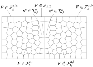
Figure 1: Explanation of the employed notation for mesh elements and faces, in a two-dimensional setting. The left domain is elastic, the right one acoustic.

We can now proceed to state the main assumptions on $\mathcal{T}_{h}$, referring to [16] for further details.

Assumption 1a.

Given an element $\kappa\in\mathcal{T}_{h}$, there exists a set of nonoverlapping (not necessarily shape-regular) $d$-dimensional simplices $\{\kappa_{\flat}^{F}\}_{F\subset\partial\kappa}\subset\kappa$, such that, for any face $F\subset\partial\kappa$,

$$(\mathrm{i})\ \displaystyle h_{\kappa}\lesssim\frac{d|\kappa_{\flat}^{F}|}{|F|},\qquad(\mathrm{ii})\ \displaystyle\bigcup_{F\subset\partial\kappa}\overline{\kappa}_{\flat}^{F}\subseteq\overline{\kappa},$$

where the hidden constant is independent of the discretization parameters, the number of faces of $\kappa$, the measure of $F$, and the material properties.

Remark 2.1 (Number of faces and degenerating faces).

Notice that no restriction is imposed by Assumption 1a on either the number of faces of an element, or the measure of the face of an element with respect to the diameter of the element itself. Therefore, the case of faces degenerating under mesh refinement can be considered as well, cf. also [16, 7].

We recall that, under Assumption 1a, the following trace-inverse inequality holds for polytopic elements:

$$\forall\kappa\in\mathcal{T}_{h},\,\forall v\in\mathscr{P}_{p}(\kappa),\quad\|v\|_{L^{2}(\partial\kappa)}\lesssim ph_{\kappa}^{-\nicefrac{{1}}{{2}}}\|v\|_{L^{2}(\kappa)},$$ (16)

where the hidden constant is independent of the discretization parameters, the number of faces per element, and the material properties [16].

Assumption 1b.

Let $\mathcal{T}_{h}^{\sharp}=\{\mathcal{K}\}$ denote a covering of $\Omega={\Omega_{e}}\cup{\Omega_{a}}$ consisting of shape-regular $d$-dimensional simplices $\mathcal{K}$. We assume that, for any $\kappa\in\mathcal{T}_{h}$, there exists $\mathcal{K}\in\mathcal{T}_{h}^{\sharp}$ such that $\kappa\subset\mathcal{K}$ and

$$\max_{\kappa\in\mathcal{T}_{h}}\operatorname{card}\left\{\kappa^{\prime}\in\mathcal{T}_{h}:\kappa^{\prime}\cap\mathcal{K}\neq\emptyset,\ \mathcal{K}\in\mathcal{T}_{h}^{\sharp}\hbox{ such that }\kappa\subset\mathcal{K}\right\}\lesssim 1;$$

and that, for each pair $\kappa\in\mathcal{T}_{h}$, $\mathcal{K}\in\mathcal{T}_{h}^{\sharp}$ with $\kappa\subset\mathcal{K}$,

$$\hbox{diam}(\mathcal{K})\lesssim h_{\kappa},$$

where the hidden constant is independent of the discretization parameters and of the material properties [11, 16].

Assumption 1c.

Let $\kappa^{+},\kappa^{-}$ be any two neighboring elements of $\mathcal{T}_{h}$. We assume the following $hp$-local bounded variation property for both the meshsize and the polynomial degree:

$$h_{\kappa^{+}}\lesssim h_{\kappa^{-}}\lesssim h_{\kappa^{+}},\quad p_{\kappa^{+}}\lesssim p_{\kappa^{-}}\lesssim p_{\kappa^{+}},$$

where the hidden constant is independent of the discretization parameters, the number of faces per element, and the material properties [61, 62].

3 Semi-discrete problem

Before stating the dG formulation of the semi-discrete problem we introduce the following average and jump operators [1, 63]. For sufficiently smooth scalar-, vector- and tensor-valued fields $\psi$, $\mathbf{v}$, and $\mathbf{\tau}$, we define averages and jumps on an internal face $F\in\mathcal{F}_{h}^{e,\mathrm{i}}\cup\mathcal{F}_{h}^{a,\mathrm{i}}$, $F\subset\partial\kappa^{+}\cap\partial\kappa^{-}$ with $\kappa^{+}$ and $\kappa^{-}$ any two neighboring elements in $\mathcal{T}_{h}^{e}$ or $\mathcal{T}_{h}^{a}$, as follows:

$${[[{\psi}]]} =\psi^{+}\mathbf{n}^{+}+\psi^{-}\mathbf{n}^{-}, \qquad{\{\{{\psi}\}\}} =\frac{\psi^{+}+\psi^{-}}{2},$$

$${[[{\mathbf{v}}]]} =\mathbf{v}^{+}\otimes\mathbf{n}^{+}+\mathbf{v}^{-}\otimes\mathbf{n}^{-}, \qquad{\{\{{\mathbf{v}}\}\}} =\frac{\mathbf{v}^{+}+\mathbf{v}^{-}}{2},$$

$${[[{\mathbf{\tau}}]]} =\mathbf{\tau}^{+}\mathbf{n}^{+}+\mathbf{\tau}^{-}\mathbf{n}^{-}, \qquad{\{\{{\mathbf{\tau}}\}\}} =\frac{\mathbf{\tau}^{+}+\mathbf{\tau}^{-}}{2},$$

where $\mathbf{a}\otimes\mathbf{b}$ denotes the tensor product of $\mathbf{a},\mathbf{b}\in\mathbb{R}^{3}$, and $\psi^{\pm}$, $\mathbf{v}^{\pm}$ and $\mathbf{\tau}^{\pm}$ denote the traces of $\psi$, $\mathbf{v}$ and $\mathbf{\tau}$ on $F$ taken from the interior of $\kappa^{\pm}$, and $\mathbf{n}^{\pm}$ is the outer unit normal vector to $\partial\kappa^{\pm}$. When considering a boundary face $F\in\mathcal{F}_{h}^{e,\mathrm{b}}\cup\mathcal{F}_{h}^{a,\mathrm{b}}$, we set ${[[{\psi}]]}=\psi\mathbf{n}$, ${[[{\mathbf{v}}]]}=\mathbf{v}\otimes\mathbf{n}$, ${[[{\mathbf{\tau}}]]}=\mathbf{\tau}\mathbf{n}$, and ${\{\{{\psi}\}\}}=\psi$, ${\{\{{\mathbf{v}}\}\}}=\mathbf{v}$, ${\{\{{\mathbf{\tau}}\}\}}=\mathbf{\tau}$. We also use the shorthand notation

$$\left\langle\Phi,\Psi\right\rangle_{\mathcal{F}}=\sum_{F\in\mathcal{F}}(\Phi,\Psi)_{F},\qquad\|\Phi\|_{\mathcal{F}}=\left\langle\Phi,\Phi\right\rangle_{\mathcal{F}}^{\nicefrac{{1}}{{2}}}$$

for scalar, vector or tensor fields $\Phi$ and $\Psi$ and for a generic collection of faces $\mathcal{F}\subset\mathcal{F}_{h}$.

The semi-discrete approximation of problem (11) reads: find $(\mathbf{u}_{h},\varphi_{h})\!\in\!C^{2}([0,T];\!\mathbf{V}_{\!h}^{e})\times C^{2}([0,T];\!V_{h}^{a})$ such that, for all $(\mathbf{v}_{h},\psi_{h})\in\mathbf{V}_{\!h}^{e}\times V_{h}^{a}$,

$$\begin{multlined}(\rho_{e}\accentset{\mbox{\footnotesize..}}{\mathbf{u}}_{h}(t),\mathbf{v}_{h})_{\Omega_{e}}+(c^{-2}\rho_{a}\accentset{\mbox{\footnotesize..}}{\varphi}_{h}(t),\psi_{h})_{\Omega_{a}}+(2\rho\zeta\accentset{\mbox{\footnotesize.}}{\mathbf{u}}_{h}(t),\mathbf{v}_{h})_{\Omega_{e}}+(\rho\zeta^{2}\mathbf{u}_{h}(t),\mathbf{v}_{h})_{\Omega_{e}}\\[5.0pt] +\mathcal{A}_{h}^{e}(\mathbf{u}_{h}(t),\mathbf{v}_{h})+\mathcal{A}_{h}^{a}(\varphi_{h}(t),\psi_{h})+\mathcal{I}_{h}^{e}(\accentset{\mbox{\footnotesize.}}{\varphi}_{h}(t),\mathbf{v}_{h})+\mathcal{I}_{h}^{a}(\accentset{\mbox{\footnotesize.}}{\mathbf{u}}_{h}(t),\psi_{h})\\ =({\mathbf{f}_{e}}(t),\mathbf{v}_{h})_{\Omega_{e}}+(\rho_{a}f_{a}(t),\psi_{h})_{\Omega_{a}},\end{multlined}(\rho_{e}\accentset{\mbox{\footnotesize..}}{\mathbf{u}}_{h}(t),\mathbf{v}_{h})_{\Omega_{e}}+(c^{-2}\rho_{a}\accentset{\mbox{\footnotesize..}}{\varphi}_{h}(t),\psi_{h})_{\Omega_{a}}+(2\rho\zeta\accentset{\mbox{\footnotesize.}}{\mathbf{u}}_{h}(t),\mathbf{v}_{h})_{\Omega_{e}}+(\rho\zeta^{2}\mathbf{u}_{h}(t),\mathbf{v}_{h})_{\Omega_{e}}\\[5.0pt] +\mathcal{A}_{h}^{e}(\mathbf{u}_{h}(t),\mathbf{v}_{h})+\mathcal{A}_{h}^{a}(\varphi_{h}(t),\psi_{h})+\mathcal{I}_{h}^{e}(\accentset{\mbox{\footnotesize.}}{\varphi}_{h}(t),\mathbf{v}_{h})+\mathcal{I}_{h}^{a}(\accentset{\mbox{\footnotesize.}}{\mathbf{u}}_{h}(t),\psi_{h})\\ =({\mathbf{f}_{e}}(t),\mathbf{v}_{h})_{\Omega_{e}}+(\rho_{a}f_{a}(t),\psi_{h})_{\Omega_{a}},$$ (20)

with initial conditions $\left({\mathbf{u}_{h}(0),\accentset{\mbox{\footnotesize.}}{\mathbf{u}}_{h}(0),\varphi_{h}(0),\accentset{\mbox{\footnotesize.}}{\varphi}_{h}(0)}\right)\in\mathbf{V}_{\!h}^{e}\times\mathbf{V}_{\!h}^{e}\times V_{h}^{a}\times V_{h}^{a}$, where the bilinear forms $\mathcal{A}_{h}\colon\mathbf{V}_{\!h}^{e}\times\mathbf{V}_{\!h}^{e}\to\mathbb{R}$, $\mathcal{A}_{h}^{a}\colon V_{h}^{a}\times V_{h}^{a}\to\mathbb{R}$, $\mathcal{I}_{h}^{e}\colon V_{h}^{a}\times\mathbf{V}_{\!h}^{e}\to\mathbb{R}$ and $\mathcal{I}_{h}^{a}\colon\mathbf{V}_{\!h}^{e}\times V_{h}^{a}\to\mathbb{R}$ are given by

$$\mathcal{A}_{h}^{e}(\mathbf{u},\mathbf{v})= \ (\bm{\sigma}_{h}(\mathbf{u}),\bm{\varepsilon}_{h}(\mathbf{v}))_{\Omega_{e}}-\left\langle{\{\{{\bm{\sigma}_{h}(\mathbf{u})}\}\}},{[[{\mathbf{v}}]]}\right\rangle_{{\mathcal{F}}_{h}^{e}}-\left\langle{[[{\mathbf{u}}]]},{\{\{{\bm{\sigma}_{h}(\mathbf{v})}\}\}}\right\rangle_{{\mathcal{F}}_{h}^{e}}+\left\langle\eta{[[{\mathbf{u}}]]},{[[{\mathbf{v}}]]}\right\rangle_{{\mathcal{F}}_{h}^{e}}$$ (21)

$$\mathcal{A}_{h}^{a}(\varphi,\psi)= \ (\rho_{a}\mathbf{\nabla}_{h}\varphi,\mathbf{\nabla}_{h}\psi)_{\Omega_{a}}-\left\langle{\{\{{\rho_{a}\mathbf{\nabla}_{h}\varphi}\}\}},{[[{\psi}]]}\right\rangle_{{\mathcal{F}}_{h}^{a}}-\left\langle{[[{\varphi}]]},{\{\{{\rho_{a}\mathbf{\nabla}_{h}\psi}\}\}}\right\rangle_{{\mathcal{F}}_{h}^{a}}+\left\langle\chi{[[{\varphi}]]},{[[{\psi}]]}\right\rangle_{{\mathcal{F}}_{h}^{a}}$$

$$\mathcal{I}_{h}^{e}(\psi,\mathbf{v})= \ (\rho_{a}\psi\mathbf{n}_{e},\mathbf{v})_{\Gamma_{\mathrm{I}}},\quad\mathcal{I}_{h}^{a}(\mathbf{v},\psi)=({\rho_{a}\mathbf{v}}\raisebox{-0.86108pt}{\scalebox{1.3}{$\cdot$}}{\mathbf{n}_{a}},\psi)_{\Gamma_{\mathrm{I}}}=-\mathcal{I}_{h}^{e}(\psi,\mathbf{v}),$$

with $\mathbf{\nabla}_{h}$ the usual broken gradient operator on $\mathcal{T}_{h}$. We point out that the last identity in (21) holds due to the fact that $\mathbf{n}_{a}=-\mathbf{n}_{e}$. Here we have set, for any integer $l\geq 1$ and any $\mathbf{v}\in\mathbf{H}^{l}(\mathcal{T}_{h}^{e})\supset\mathbf{V}_{\!h}^{e}$,

$$\bm{\varepsilon}_{h}(\mathbf{v})=\frac{1}{2}\left(\mathbf{\nabla}_{h}\mathbf{v}+\mathbf{\nabla}_{h}\mathbf{v}^{T}\right),\quad\bm{\sigma}_{h}(\mathbf{v})=\mathbb{C}\bm{\varepsilon}_{h}(\mathbf{v}).$$

The stabilization functions $\eta\in L^{\infty}({\mathcal{F}}_{h}^{e})$ and $\chi\in L^{\infty}({\mathcal{F}}_{h}^{a})$ are defined as follows:

$$\eta_{|F} =\begin{cases}\displaystyle\alpha\max_{\kappa\in\{\kappa^{+},\kappa^{-}\}}\left(\frac{\overline{\mathbb{C}}_{\kappa}p^{2}_{e,\kappa}}{h_{\kappa}}\right)&\quad\forall F\in{\mathcal{F}}_{h}^{e,\mathrm{i}},\quad\ F\subseteq\partial{\kappa^{+}}\cap\partial{\kappa^{-}},\\[15.0pt] \displaystyle\frac{\overline{\mathbb{C}}_{\kappa}p^{2}_{e,\kappa}}{h_{\kappa}}&\quad\forall F\in{\mathcal{F}}_{h}^{e,\mathrm{b}},\quad F\subseteq\partial\kappa;\end{cases}$$ (22a)

$$\chi_{|F} =\begin{cases}\displaystyle\beta\max_{\kappa\in\{\kappa^{+},\kappa^{-}\}}\left(\frac{\overline{\rho}_{a,\kappa}p_{a,\kappa}^{2}}{h_{\kappa}}\right)&\ \,\forall F\in{\mathcal{F}}_{h}^{a,\mathrm{i}},\quad\,F\subseteq\partial{\kappa^{+}}\cap\partial{\kappa^{-}},\\[15.0pt] \displaystyle\frac{\overline{\rho}_{a,\kappa}p_{a,\kappa}^{2}}{h_{\kappa}}&\ \,\forall F\in{\mathcal{F}}_{h}^{a,\mathrm{b}},\quad F\subseteq\partial\kappa.\end{cases}$$ (22b)

where $\alpha,\beta>0$ are positive constants to be properly chosen. We now introduce the following norms:

$$\|\mathbf{v}\|_{{\mathrm{dG}},e}^{2} =\|\mathbb{C}^{\nicefrac{{1}}{{2}}}\bm{\varepsilon}_{h}(\mathbf{v})\|_{\Omega_{e}}^{2}+\|{\eta^{\nicefrac{{1}}{{2}}}{[[{\mathbf{v}}]]}}\|_{{\mathcal{F}}_{h}^{e}}^{2} \forall\mathbf{v}\in\mathbf{H}^{1}(\mathcal{T}_{h}^{e})\supset\mathbf{V}_{\!h}^{e},$$ (23)

$$\vvvert\mathbf{v}\vvvert_{{\mathrm{dG}},e}^{2} =\|\mathbf{v}\|_{\mathrm{dG},e}^{2}+\|{\eta^{-\nicefrac{{1}}{{2}}}{\{\{{\mathbb{C}\bm{\varepsilon}_{h}(\mathbf{v})}\}\}}}\|_{{\mathcal{F}}_{h}^{e}}^{2} \forall\mathbf{v}\in\mathbf{H}^{2}(\mathcal{T}_{h}^{e}),$$

$$\|\psi\|_{{\mathrm{dG}},a}^{2} =\|\rho_{a}^{\nicefrac{{1}}{{2}}}\mathbf{\nabla}_{h}\psi\|_{{\Omega_{a}}}^{2}+\|{\chi^{\nicefrac{{1}}{{2}}}{[[{\psi}]]}}\|_{{\mathcal{F}}_{h}^{a}}^{2} \forall\psi\in H^{1}(\mathcal{T}_{h}^{a})\supset V_{h}^{a},$$

$$\vvvert\psi\vvvert_{{\mathrm{dG},a}}^{2} =\|\psi\|_{\mathrm{dG},a}^{2}+\|{\chi^{-\nicefrac{{1}}{{2}}}{\{\{{\rho_{a}\mathbf{\nabla}_{h}\psi}\}\}}}\|_{{\mathcal{F}}_{h}^{a}}^{2} \forall\psi\in H^{2}(\mathcal{T}_{h}^{a}).$$

The following result follows based on employing standard arguments.

Lemma 3.1 (Coercivity and boundedness of $\mathcal{A}_{h}^{e}$ and $\mathcal{A}_{h}^{a}$).

Provided that $\mathcal{T}_{h}$ satisfies Assumption 1a, and that constants $\alpha$ and $\beta$ in (22a)–(22b) are chosen sufficiently large, the following continuity and coercivity bounds hold:

$$\mathcal{A}_{h}^{e}(\mathbf{u},\mathbf{v}) \lesssim\|\mathbf{u}\|_{{\mathrm{dG}},e}\|\mathbf{v}\|_{{\mathrm{dG}},e} \forall\mathbf{u},\mathbf{v}\in\mathbf{V}_{\!h}^{e},$$ (24a)

$$\mathcal{A}_{h}^{e}(\mathbf{v},\mathbf{v}) \gtrsim\|\mathbf{v}\|_{{\mathrm{dG}},e}^{2} \forall\mathbf{v}\in\mathbf{V}_{\!h}^{e},$$

$$\mathcal{A}_{h}^{a}(\varphi,\psi) \lesssim\|\varphi\|_{{\mathrm{dG}},a}\|\psi\|_{{\mathrm{dG}},a} \forall\varphi,\psi\in V_{h}^{a},$$ (24b)

$$\mathcal{A}_{h}^{a}(\psi,\psi) \gtrsim\|\psi\|_{{\mathrm{dG}},a}^{2} \forall\psi\in V_{h}^{a}.$$

Moreover,

$$\mathcal{A}_{h}^{e}(\mathbf{w},\mathbf{v}) \lesssim{\vvvert{\mathbf{w}}\vvvert}_{{\mathrm{dG}},e}\|\mathbf{v}\|_{{\mathrm{dG}},e} \forall(\mathbf{w},\mathbf{v})\in\mathbf{H}^{2}(\mathcal{T}_{h}^{e})\times\mathbf{V}_{\!h}^{e},$$ (25)

$$\mathcal{A}_{h}^{a}(\varphi,\psi) \lesssim{\vvvert{\varphi}\vvvert}_{{\mathrm{dG}},a}\|\psi\|_{{\mathrm{dG}},a} \forall(\varphi,\psi)\in H^{2}(\mathcal{T}_{h}^{a})\times V_{h}^{a}.$$

As a consequence of (24a)–(24b), whose proof hinges on Lemma A1, the theory of ordinary differential equations guarantees that problem (20) is well-posed (notice, also, that the coupling terms stemming from bilinear forms $\mathcal{I}_{h}^{e}$ and $\mathcal{I}_{h}^{a}$ do not contribute to the energy of the system, cf. Remark 4.1 below).

4 Stability of the semi-discrete formulation

In this section we prove a stability result for the semi-discrete problem (20) (see [9, 62, 64, 65] for the purely elastic case). Let $\mathbf{W}=(\mathbf{v},\psi)\in C^{1}([0,T];\mathbf{V}_{\!h}^{e})\times C^{1}([0,T];V_{h}^{a})$; we introduce the following mesh-dependent energy norm

$$\|{\mathbf{W}}(t)\|_{\mathcal{E}}^{2}=\|\mathbf{v}(t)\|_{{\mathcal{E}}_{e}}^{2}+\|\psi(t)\|_{{\mathcal{E}}_{a}}^{2},$$ (26)

where

$$\|\mathbf{v}(t)\|_{{\mathcal{E}}_{e}}^{2} =\|\rho_{e}^{\nicefrac{{1}}{{2}}}\accentset{\mbox{\footnotesize.}}{\mathbf{v}}(t)\|_{\Omega_{e}}^{2}+\|\rho_{e}^{\nicefrac{{1}}{{2}}}\zeta\mathbf{v}(t)\|_{\Omega_{e}}^{2}+\|\mathbf{v}(t)\|_{\mathrm{dG},e}^{2},$$ (27)

$$\|\psi(t)\|_{{\mathcal{E}}_{a}}^{2} =\|c^{-1}\rho_{a}^{\nicefrac{{1}}{{2}}}\accentset{\mbox{\footnotesize.}}{\psi}(t)\|_{\Omega_{a}}^{2}+\|\psi(t)\|_{\mathrm{dG},a}^{2}.$$

Remark 4.1 (Energy norm).

The definition of the energy norm does not take into account the interface terms. The reason is related to the fact that, as observed previously, the bilinear forms $\mathcal{I}_{h}^{e}$ and $\mathcal{I}_{h}^{a}$ are skew-symmetric, i.e., $\mathcal{I}_{h}^{a}(\mathbf{v},\psi)=-\mathcal{I}_{h}^{e}(\psi,\mathbf{v})$ for all $(\mathbf{v},\psi)\in\mathbf{V}_{\!h}^{e}\times V_{h}^{a}$.

Theorem 4.2 (Stability of the semi-discrete formulation).

Let $\mathbf{U}_{h}=(\mathbf{u}_{h},\varphi_{h})$ be the solution of (20). For sufficiently large penalty parameters $\alpha$ and $\beta$ in (22a) and (22b), respectively, the following bound holds:

$$\|{\mathbf{U}}_{h}(t)\|_{\mathcal{E}}\lesssim\|{\mathbf{U}}_{h}(0)\|_{\mathcal{E}}+\int_{0}^{t}\left(\|{\mathbf{f}_{e}}(\tau)\|_{\Omega_{e}}+\|f_{a}(\tau)\|_{\Omega_{a}}\right)\,\mathrm{d}\tau,\quad t\in(0,T].$$ (28)

Proof.

Taking $\mathbf{v}_{h}=\accentset{\mbox{\footnotesize.}}{\mathbf{u}}_{h}$ and $\psi_{h}=\accentset{\mbox{\footnotesize.}}{\varphi}_{h}$ in (20), we obtain

$$(\rho_{e}\accentset{\mbox{\footnotesize..}}{\mathbf{u}}_{h},\accentset{\mbox{\footnotesize.}}{\mathbf{u}}_{h})_{\Omega_{e}}+(2\rho_{e}\zeta\accentset{\mbox{\footnotesize.}}{\mathbf{u}}_{h},\accentset{\mbox{\footnotesize.}}{\mathbf{u}}_{h})_{\Omega_{e}}+(\rho_{e}\zeta^{2}\mathbf{u}_{h},\accentset{\mbox{\footnotesize.}}{\mathbf{u}}_{h})_{\Omega_{e}}+\big{(}\bm{\sigma}_{h}(\mathbf{u}_{h}),\bm{\varepsilon}_{h}(\accentset{\mbox{\footnotesize.}}{\mathbf{u}}_{h})\big{)}_{\Omega_{e}}\\ -\left\langle{\{\{{\bm{\sigma}_{h}(\mathbf{u}_{h})}\}\}},{[[{\accentset{\mbox{\footnotesize.}}{\mathbf{u}}_{h}}]]}\right\rangle_{{\mathcal{F}}_{h}^{e}}-\left\langle{[[{\mathbf{u}_{h}}]]},{\{\{{\bm{\sigma}_{h}(\accentset{\mbox{\footnotesize.}}{\mathbf{u}}_{h})}\}\}}\right\rangle_{{\mathcal{F}}_{h}^{e}}+\left\langle\eta{[[{\mathbf{u}_{h}}]]},{[[{\accentset{\mbox{\footnotesize.}}{\mathbf{u}}_{h}}]]}\right\rangle_{{\mathcal{F}}_{h}^{e}}\\ +(c^{-2}\rho_{a}\accentset{\mbox{\footnotesize..}}{\varphi}_{h},\accentset{\mbox{\footnotesize.}}{\varphi}_{h})_{\Omega_{a}}+(\rho_{a}\mathbf{\nabla}_{h}\varphi_{h},\mathbf{\nabla}_{h}\accentset{\mbox{\footnotesize.}}{\varphi}_{h})_{\Omega_{a}}-\left\langle{\{\{{\rho_{a}\mathbf{\nabla}_{h}\varphi_{h}}\}\}},{[[{\accentset{\mbox{\footnotesize.}}{\varphi}_{h}}]]}\right\rangle_{{\mathcal{F}}_{h}^{a}}\\ -\left\langle\rho_{a}{[[{\varphi_{h}}]]},{\{\{{\mathbf{\nabla}_{h}\accentset{\mbox{\footnotesize.}}{\varphi}_{h}}\}\}}\right\rangle_{{\mathcal{F}}_{h}^{a}}+\left\langle\chi{[[{\varphi_{h}}]]},{[[{\accentset{\mbox{\footnotesize.}}{\varphi}_{h}}]]}\right\rangle_{{\mathcal{F}}_{h}^{a}}=({\mathbf{f}_{e}},\accentset{\mbox{\footnotesize.}}{\mathbf{u}}_{h})_{\Omega_{e}}+(\rho_{a}f_{a},\accentset{\mbox{\footnotesize.}}{\varphi}_{h})_{\Omega_{a}},$$

that is,

$$\frac{1}{2}\frac{\mathrm{d}}{\mathrm{d}t}\left(\|{\mathbf{U}}_{h}\|_{\mathcal{E}}^{2}-2\left(\left\langle{\{\{{\bm{\sigma}_{h}(\mathbf{u}_{h})}\}\}},{[[{\mathbf{u}_{h}}]]}\right\rangle_{{\mathcal{F}}_{h}^{e}}+\left\langle{\{\{{\rho_{a}\mathbf{\nabla}_{h}\varphi_{h}}\}\}},{[[{\varphi_{h}}]]}\right\rangle_{{\mathcal{F}}_{h}^{a}}\right)\right)\\ +2\|\rho_{e}^{\nicefrac{{1}}{{2}}}\zeta^{\nicefrac{{1}}{{2}}}\accentset{\mbox{\footnotesize.}}{\mathbf{u}}_{h}\|_{\Omega_{e}}^{2}=({\mathbf{f}_{e}},\accentset{\mbox{\footnotesize.}}{\mathbf{u}}_{h})_{\Omega_{e}}+(\rho_{a}{f_{a}},\accentset{\mbox{\footnotesize.}}{\varphi}_{h})_{\Omega_{a}}.$$

Integrating the above identity over the interval $(0,t)$ we have

$$\|{\mathbf{U}}_{h}(t)\|_{\mathcal{E}}^{2}-2\left(\left\langle{\{\{{\bm{\sigma}_{h}(\mathbf{u}_{h}(t))}\}\}},{[[{\mathbf{u}_{h}(t)}]]}\right\rangle_{{\mathcal{F}}_{h}^{e}}+\left\langle{\{\{{\rho_{a}\mathbf{\nabla}_{h}\varphi_{h}(t)}\}\}},{[[{\varphi_{h}(t)}]]}\right\rangle_{{\mathcal{F}}_{h}^{a}}\right)\\ +\,4\!\int_{0}^{t}\|\rho_{e}^{\nicefrac{{1}}{{2}}}\zeta^{\nicefrac{{1}}{{2}}}\accentset{\mbox{\footnotesize.}}{\mathbf{u}}_{h}(\tau)\|_{\Omega_{e}}^{2}\mathrm{d}\tau=\|{\mathbf{U}}_{h}(0)\|_{\mathcal{E}}^{2}-2\left(\left\langle{\{\{{\bm{\sigma}_{h}(\mathbf{u}_{h}(0))}\}\}},{[[{\mathbf{u}_{h}(0)}]]}\right\rangle_{{\mathcal{F}}_{h}^{e}}\right.\\ +\left.\left\langle{\{\{{\rho_{a}\mathbf{\nabla}_{h}\varphi_{h}(0)}\}\}},{[[{\varphi_{h}(0)}]]}\right\rangle_{{\mathcal{F}}_{h}^{a}}\right)+2\int_{0}^{t}\!\big{(}{\mathbf{f}_{e}}(\tau),\accentset{\mbox{\footnotesize.}}{\mathbf{u}}_{h}(\tau)\big{)}_{\Omega_{e}}\mathrm{d}\tau+2\int_{0}^{t}\!\big{(}\rho_{a}{f_{a}}(\tau),\accentset{\mbox{\footnotesize.}}{\varphi}_{h}(\tau)\big{)}_{\Omega_{a}}\mathrm{d}\tau,$$

and, since the last term on the left-hand side is positive, we get

$$\|{\mathbf{U}}_{h}(t)\|_{\mathcal{E}}^{2}-2\left(\left\langle{\{\{{\bm{\sigma}_{h}(\mathbf{u}_{h}(t))}\}\}},{[[{\mathbf{u}_{h}(t)}]]}\right\rangle_{{\mathcal{F}}_{h}^{e}}+\left\langle{\{\{{\rho_{a}\mathbf{\nabla}_{h}\varphi_{h}(t)}\}\}},{[[{\varphi_{h}(t)}]]}\right\rangle_{{\mathcal{F}}_{h}^{a}}\right)\\ \leq\|{\mathbf{U}}_{h}(0)\|_{\mathcal{E}}^{2}-2\left(\left\langle{\{\{{\bm{\sigma}_{h}(\mathbf{u}_{h}(0))}\}\}},{[[{\mathbf{u}_{h}(0)}]]}\right\rangle_{{\mathcal{F}}_{h}^{e}}+\left\langle{\{\{{\rho_{a}\mathbf{\nabla}_{h}\varphi_{h}(0)}\}\}},{[[{\varphi_{h}(0)}]]}\right\rangle_{{\mathcal{F}}_{h}^{a}}\right)\\ +2\int_{0}^{t}\!\big{(}{\mathbf{f}_{e}}(\tau),\accentset{\mbox{\footnotesize.}}{\mathbf{u}}_{h}(\tau)\big{)}_{\Omega_{e}}\,\mathrm{d}\tau+2\int_{0}^{t}\!\big{(}\rho_{a}{f_{a}}(\tau),\accentset{\mbox{\footnotesize.}}{\varphi}_{h}(\tau)\big{)}_{\Omega_{a}}\,\mathrm{d}\tau.$$

From Lemma A2 in the Appendix, we get

$$\|{\mathbf{U}}_{h}(t)\|_{\mathcal{E}}^{2}-2\left(\left\langle{\{\{{\bm{\sigma}_{h}(\mathbf{u}_{h}(t))}\}\}},{[[{\mathbf{u}_{h}(t)}]]}\right\rangle_{{\mathcal{F}}_{h}^{e}}+\left\langle{\{\{{\rho_{a}\mathbf{\nabla}_{h}\varphi_{h}(t)}\}\}},{[[{\varphi_{h}(t)}]]}\right\rangle_{{\mathcal{F}}_{h}^{a}}\right) \gtrsim\|{\mathbf{U}}_{h}(t)\|_{\mathcal{E}}^{2},$$

$$\|{\mathbf{U}}_{h}(0)\|_{\mathcal{E}}^{2}-2\left(\left\langle{\{\{{\bm{\sigma}_{h}(\mathbf{u}_{h}(0))}\}\}},{[[{\mathbf{u}_{h}(0)}]]}\right\rangle_{{\mathcal{F}}_{h}^{e}}+\,\left\langle{\{\{{\rho_{a}\mathbf{\nabla}_{h}\varphi_{h}(0)}\}\}},{[[{\varphi_{h}(0)}]]}\right\rangle_{{\mathcal{F}}_{h}^{a}}\right) \lesssim\|{\mathbf{U}}_{h}(0)\|_{\mathcal{E}}^{2},$$

where the first bound holds if the stability parameters $\alpha$ and $\beta$ are chosen large enough. Consequently

$$\|{\mathbf{U}}_{h}(t)\|_{\mathcal{E}}^{2} \lesssim\|{\mathbf{U}}_{h}(0)\|_{\mathcal{E}}^{2}+2\int_{0}^{t}\big{(}{\mathbf{f}_{e}}(\tau),\accentset{\mbox{\footnotesize.}}{\mathbf{u}}_{h}(\tau)\big{)}_{\Omega_{e}}\,\mathrm{d}\tau+2\int_{0}^{t}\big{(}\rho_{a}{f_{a}}(\tau),\accentset{\mbox{\footnotesize.}}{\varphi}_{h}(\tau)\big{)}_{\Omega_{a}}\,\mathrm{d}\tau$$

$$\lesssim\|{\mathbf{U}}_{h}(0)\|_{\mathcal{E}}^{2}+\int_{0}^{t}\|{\mathbf{f}_{e}}(\tau)\|_{\Omega_{e}}\|\rho_{e}^{\nicefrac{{1}}{{2}}}\accentset{\mbox{\footnotesize.}}{\mathbf{u}}_{h}(\tau)\|_{\Omega_{e}}+\int_{0}^{t}\|{f_{a}}(\tau)\|_{\Omega_{a}}\|c^{-1}\rho_{a}^{\nicefrac{{1}}{{2}}}\accentset{\mbox{\footnotesize.}}{\varphi}_{h}(\tau)\|_{\Omega_{a}}$$

$$\lesssim\|{\mathbf{U}}_{h}(0)\|_{\mathcal{E}}^{2}+\int_{0}^{t}\left(\|{\mathbf{f}_{e}}(\tau)\|_{\Omega_{e}}+\|f_{a}(\tau)\|_{\Omega_{a}}\right)\|{\mathbf{U}}_{h}(\tau)\|_{\mathcal{E}}\,\mathrm{d}\tau,$$

where we have used the Cauchy–Schwarz inequality and the definition (26) of the energy norm in the last two bounds. The assertion follows then by employing Gronwall’s Lemma (see e.g. [66, p. 28]). ∎

5 Semi-discrete error estimate

The main subject of this section is the derivation of an a priori error estimate for the semi-discrete coupled problem (20).

For an open bounded polytopic domain $D\subset\mathbb{R}^{d}$, and a generic polytopic mesh $\mathcal{T}_{h}$ over $D$, we introduce, for any $\kappa\in\mathcal{T}_{h}$ and $m\in\mathbb{N}_{0}$, the extension operator ${\mathscr{E}}\colon H^{m}(\kappa)\to H^{m}(\mathbb{R}^{d})$ such that $\mathscr{E}v_{|\kappa}=v$, $\|\mathscr{E}v\|_{H^{m}(\mathbb{R}^{d})}\leq C\|v\|_{H^{m}(\kappa)}$, with $C>0$ depending only on $m$ and $\kappa$. The corresponding vector-valued version, mapping $\mathbf{H}^{m}(\kappa)$ onto $\mathbf{H}^{m}(\mathbb{R}^{d})$, acts component-wise and will be denoted in the same way. The result below is a consequence of the $hp$-approximation properties stated in [16, Lemmas 23 and 33] and of Assumption 1c on local bounded variation.

Lemma 5.1 (Interpolation estimates).

For any pair of functions $(\mathbf{v},\psi)\in\mathbf{H}^{m}(\mathcal{T}_{h}^{e})\times H^{n}(\mathcal{T}_{h}^{a})$, $m\geq 2$, $n\geq 2$, there exists a pair of interpolants $(\mathbf{v}_{I},\psi_{I})\in\mathbf{V}_{\!h}^{e}\times V_{h}^{a}$ such that

$$\vvvert{\mathbf{v}-\mathbf{v}_{I}}\vvvert_{\mathrm{dG},e}^{2} \lesssim\sum_{\kappa\in\mathcal{T}_{h}^{e}}\frac{h_{\kappa}^{2\min(m,p_{e,\kappa}+1)-2}}{p_{e,\kappa}^{2m-3}}\|\mathscr{E}\mathbf{v}\|^{2}_{m,\mathcal{K}},$$

$$\vvvert{\psi-\psi_{I}}\vvvert_{\mathrm{dG},a}^{2} \lesssim\sum_{\kappa\in\mathcal{T}_{h}^{a}}\frac{h_{\kappa}^{2\min(n,p_{a,\kappa}+1)-2}}{p_{a,\kappa}^{2n-3}}\|\mathscr{E}\psi\|^{2}_{n,\mathcal{K}}.$$

Additionally, if $({\mathbf{v}},\psi)\in C^{1}([0,T];\mathbf{H}^{m}(\mathcal{T}_{h}^{e}))\times C^{1}([0,T];H^{n}(\mathcal{T}_{h}^{a}))$, $m\geq 2$, $n\geq 2$, then

$$\|\mathbf{v}-\mathbf{v}_{I}\|_{{\mathcal{E}}_{e}}^{2} \lesssim\sum_{\kappa\in\mathcal{T}_{h}^{e}}\!\frac{h_{\kappa}^{2\min(m,p_{e,\kappa}+1)-2}}{p_{e,\kappa}^{2m-3}}\left(\|\mathscr{E}\accentset{\mbox{\footnotesize.}}{\mathbf{v}}\|_{m,\mathcal{K}}^{2}+\|\mathscr{E}\mathbf{v}\|_{m,\mathcal{K}}^{2}\right),$$

$$\|\psi-\psi_{I}\|_{{\mathcal{E}}_{a}}^{2} \lesssim\sum_{\kappa\in\mathcal{T}_{h}^{a}}\!\frac{h_{\kappa}^{2\min(n,p_{a,\kappa}+1)-2}}{p_{a,\kappa}^{2n-3}}\left(\|\mathscr{E}\accentset{\mbox{\footnotesize.}}{\psi}\|_{n,\mathcal{K}}^{2}+\|\mathscr{E}\psi\|_{n,\mathcal{K}}^{2}\right).$$

We are now ready to state the main result of this section.

Theorem 5.1 (A priori error estimate in the energy norm).

Let Assumptions 1a–1c hold. Assume that the exact solution of problem (1) is such that $\mathbf{u}\in C^{2}([0,T];\mathbf{H}^{m}({\Omega_{e}}))$ and $\varphi\in C^{2}([0,T];H^{n}({\Omega_{a}}))$, with $m\geq 2$, $n\geq 2$. Let $(\mathbf{u}_{h},\varphi_{h})\in C^{2}([0,T];\mathbf{V}_{\!h}^{e})\times C^{2}([0,T];V_{h}^{a})$ be the corresponding solution of the semi-discrete problem (20), with sufficiently large penalty parameters $\alpha$ and $\beta$ in (22a)–(22b). Then, the following bound holds for the discretization error $\mathbf{E}(t)=(\mathbf{e}_{e}(t),e_{a}(t))=(\mathbf{u}(t)-\mathbf{u}_{h}(t),\varphi(t)-\varphi_{h}(t))$:

$$\sup_{t\in[0,T]}\|\mathbf{E}(t)\|_{\mathcal{E}}^{2}\lesssim\sup_{t\in[0,T]}\left(\sum_{\kappa\in\mathcal{T}_{h}^{e}}\frac{h_{\kappa}^{2\min(m,p_{e,\kappa}+1)-2}}{p_{e,\kappa}^{2m-3}}\left(\|\mathscr{E}\accentset{\mbox{\footnotesize.}}{\mathbf{u}}\|_{m,\mathcal{K}}^{2}+\|\mathscr{E}\mathbf{u}\|_{m,\mathcal{K}}^{2}\right)\right.$$ (41)

$$\qquad\qquad\qquad\qquad\left.+\sum_{\kappa\in\mathcal{T}_{h}^{a}}\frac{h_{\kappa}^{2\min(n,p_{a,\kappa}+1)-2}}{p_{a,\kappa}^{2n-3}}\left(\|\mathscr{E}\accentset{\mbox{\footnotesize.}}{\varphi}\|_{n,\mathcal{K}}^{2}+\|\mathscr{E}\varphi\|_{n,\mathcal{K}}^{2}\right)\right)+$$

$$\qquad\qquad\quad\ \ +\int_{0}^{T}\!\left(\sum_{\kappa\in\mathcal{T}_{h}^{e}}\frac{h_{\kappa}^{2\min(m,p_{e,\kappa}+1)-2}}{p_{e,\kappa}^{2m-3}}\left(\|\mathscr{E}\accentset{\mbox{\footnotesize..}}{\mathbf{u}}\|_{m,\mathcal{K}}^{2}+\|\mathscr{E}\accentset{\mbox{\footnotesize.}}{\mathbf{u}}\|_{m,\mathcal{K}}^{2}+\|\mathscr{E}\mathbf{u}\|_{m,\mathcal{K}}^{2}\right)\right.$$

$$\qquad\qquad\qquad\left.+\sum_{\kappa\in\mathcal{T}_{h}^{a}}\frac{h_{\kappa}^{2\min(n,p_{a,\kappa}+1)-2}}{p_{a,\kappa}^{2n-3}}\left(\|\mathscr{E}\accentset{\mbox{\footnotesize..}}{\varphi}\|_{n,\mathcal{K}}^{2}+\|\mathscr{E}\accentset{\mbox{\footnotesize.}}{\varphi}\|_{n,\mathcal{K}}^{2}+\|\mathscr{E}\varphi\|_{n,\mathcal{K}}^{2}\right)\right)\mathrm{d}\tau.$$

Corollary 5.2 (A priori error estimate in the energy norm).

Under the hypotheses of Theorem 5.1, assume that $h\simeq h_{\kappa}$ for any $\kappa\in\mathcal{T}_{h}$, $p_{e,\kappa}=p_{e}$ for any $\kappa\in\mathcal{T}_{h}^{e}$, and $p_{a,\kappa}=p_{a}$ for any $\kappa\in\mathcal{T}_{h}^{a}$. Then, if $({\mathbf{u}},\varphi)\in C^{2}([0,T];\mathbf{H}^{m}({\Omega_{e}}))\times C^{2}([0,T];H^{n}({\Omega_{a}}))$ with $m\geq p_{e}+1$ and $n\geq p_{a}+1$, the error estimate (LABEL:eq:error-estimate) reads

$$\sup_{t\in[0,T]}\|\mathbf{E}(t)\|_{\mathcal{E}}^{2}\lesssim \ \frac{h^{2p_{e}}}{p_{e}^{2m-3}}\Bigg{(}\sup_{t\in[0,T]}\left(\|\accentset{\mbox{\footnotesize.}}{\mathbf{u}}\|_{m,{\Omega_{e}}}^{2}+\|\mathbf{u}\|_{m,{\Omega_{e}}}^{2}\right)+\int_{0}^{T}\!\!\left(\|\accentset{\mbox{\footnotesize..}}{\mathbf{u}}\|_{m,{\Omega_{e}}}^{2}+\|\accentset{\mbox{\footnotesize.}}{\mathbf{u}}\|_{m,{\Omega_{e}}}^{2}+\|\mathbf{u}\|_{m,{\Omega_{e}}}^{2}\right)\mathrm{d}t\Bigg{)}$$ (42)

$$+\frac{h^{2p_{a}}}{p_{a}^{2n-3}}\Bigg{(}\sup_{t\in[0,T]}\left(\|\accentset{\mbox{\footnotesize.}}{\varphi}\|_{n,{\Omega_{a}}}^{2}+\|\varphi\|_{n,{\Omega_{a}}}^{2}\right)+\int_{0}^{T}\!\!\big{(}\|\accentset{\mbox{\footnotesize..}}{\varphi}\|_{n,{\Omega_{a}}}^{2}+\|\accentset{\mbox{\footnotesize.}}{\varphi}\|_{n,{\Omega_{a}}}^{2}+\|\varphi\|_{n,{\Omega_{a}}}^{2}\big{)}\,\mathrm{d}t\Bigg{)}.$$

Proof of Theorem 5.1.

It is easy to see that the semi-discrete formulation (20) is strongly consistent, i.e., the exact solution $(\mathbf{u},\varphi)$ satisfies (20) for any $t\in(0,T]$:

$$\begin{multlined}(\rho_{e}\accentset{\mbox{\footnotesize..}}{\mathbf{u}},\mathbf{v})_{\Omega_{e}}+(c^{-2}\rho_{a}\accentset{\mbox{\footnotesize..}}{\varphi},\psi)_{\Omega_{a}}+(2\rho_{e}\zeta\accentset{\mbox{\footnotesize.}}{\mathbf{u}},\mathbf{v})_{\Omega_{e}}+(\rho_{e}\zeta^{2}\mathbf{u},\mathbf{v})_{\Omega_{e}}\\[4.0pt] +\mathcal{A}_{h}^{e}(\mathbf{u},\mathbf{v})+\mathcal{A}_{h}^{a}(\varphi,\psi)+\mathcal{I}_{h}^{e}(\accentset{\mbox{\footnotesize.}}{\varphi},\mathbf{v})+\mathcal{I}_{h}^{a}(\accentset{\mbox{\footnotesize.}}{\mathbf{u}},\psi)\\ \hskip 113.81102pt=({\mathbf{f}_{e}},\mathbf{v})_{\Omega_{e}}+(\rho_{a}f_{a},\psi)_{\Omega_{a}},\quad\forall(\mathbf{v},\psi)\in\mathbf{V}_{\!h}^{e}\times V_{h}^{a}.\end{multlined}(\rho_{e}\accentset{\mbox{\footnotesize..}}{\mathbf{u}},\mathbf{v})_{\Omega_{e}}+(c^{-2}\rho_{a}\accentset{\mbox{\footnotesize..}}{\varphi},\psi)_{\Omega_{a}}+(2\rho_{e}\zeta\accentset{\mbox{\footnotesize.}}{\mathbf{u}},\mathbf{v})_{\Omega_{e}}+(\rho_{e}\zeta^{2}\mathbf{u},\mathbf{v})_{\Omega_{e}}\\[4.0pt] +\mathcal{A}_{h}^{e}(\mathbf{u},\mathbf{v})+\mathcal{A}_{h}^{a}(\varphi,\psi)+\mathcal{I}_{h}^{e}(\accentset{\mbox{\footnotesize.}}{\varphi},\mathbf{v})+\mathcal{I}_{h}^{a}(\accentset{\mbox{\footnotesize.}}{\mathbf{u}},\psi)\\ \hskip 113.81102pt=({\mathbf{f}_{e}},\mathbf{v})_{\Omega_{e}}+(\rho_{a}f_{a},\psi)_{\Omega_{a}},\quad\forall(\mathbf{v},\psi)\in\mathbf{V}_{\!h}^{e}\times V_{h}^{a}.$$ (46)

Subtracting (20) from the above identity, we obtain the error equation:

$$\begin{multlined}(\rho_{e}\accentset{\mbox{\footnotesize..}}{\mathbf{e}}_{e},\mathbf{v})_{\Omega_{e}}+(c^{-2}\rho_{a}\accentset{\mbox{\footnotesize..}}{e}_{a},\psi)_{\Omega_{a}}+(2\rho_{e}\zeta\accentset{\mbox{\footnotesize.}}{\mathbf{e}}_{e},\mathbf{v})_{\Omega_{e}}+(\rho_{e}\zeta^{2}\mathbf{e}_{e},\mathbf{v})_{\Omega_{e}}\\[4.0pt] +\mathcal{A}_{h}^{e}(\mathbf{e}_{e},\mathbf{v})+\mathcal{A}_{h}^{a}(e_{a},\psi)+\mathcal{I}_{h}^{e}(\accentset{\mbox{\footnotesize.}}{e}_{a},\mathbf{v})+\mathcal{I}_{h}^{a}(\accentset{\mbox{\footnotesize.}}{\mathbf{e}}_{e},\psi)=0,\ \ \forall(\mathbf{v},\psi)\in\mathbf{V}_{\!h}^{e}\times V_{h}^{a}.\end{multlined}(\rho_{e}\accentset{\mbox{\footnotesize..}}{\mathbf{e}}_{e},\mathbf{v})_{\Omega_{e}}+(c^{-2}\rho_{a}\accentset{\mbox{\footnotesize..}}{e}_{a},\psi)_{\Omega_{a}}+(2\rho_{e}\zeta\accentset{\mbox{\footnotesize.}}{\mathbf{e}}_{e},\mathbf{v})_{\Omega_{e}}+(\rho_{e}\zeta^{2}\mathbf{e}_{e},\mathbf{v})_{\Omega_{e}}\\[4.0pt] +\mathcal{A}_{h}^{e}(\mathbf{e}_{e},\mathbf{v})+\mathcal{A}_{h}^{a}(e_{a},\psi)+\mathcal{I}_{h}^{e}(\accentset{\mbox{\footnotesize.}}{e}_{a},\mathbf{v})+\mathcal{I}_{h}^{a}(\accentset{\mbox{\footnotesize.}}{\mathbf{e}}_{e},\psi)=0,\ \ \forall(\mathbf{v},\psi)\in\mathbf{V}_{\!h}^{e}\times V_{h}^{a}.$$ (49)

We next decompose the error $\mathbf{E}=(\mathbf{e}_{e},e_{a})$ as follows: $\mathbf{E}=\mathbf{E}_{I}-\mathbf{E}_{h}$, with $\mathbf{E}_{I}=(\mathbf{e}_{I},e_{I})=(\mathbf{u}-\mathbf{u}_{I},\varphi-\varphi_{I})$, and $\mathbf{E}_{h}=(\mathbf{e}_{h},e_{h})=(\mathbf{u}_{h}-\mathbf{u}_{I},\varphi_{h}-\varphi_{I})$, $(\mathbf{u}_{I},\varphi_{I})\in\mathbf{V}_{\!h}^{e}\times V_{h}^{a}$ being the interpolants defined as in Lemma 5.1. By taking as test functions $(\mathbf{v},\psi)=(\accentset{\mbox{\footnotesize.}}{\mathbf{e}}_{h},\accentset{\mbox{\footnotesize.}}{e}_{h})$, the above identity reads then

$$(\rho_{e}\accentset{\mbox{\footnotesize..}}{\mathbf{e}}_{h},\accentset{\mbox{\footnotesize.}}{\mathbf{e}}_{h})_{\Omega_{e}}+(c^{-2}\rho_{a}\accentset{\mbox{\footnotesize..}}{e}_{h},\accentset{\mbox{\footnotesize.}}{e}_{h})_{\Omega_{a}}+(2\rho_{e}\zeta\accentset{\mbox{\footnotesize.}}{\mathbf{e}}_{h},\accentset{\mbox{\footnotesize.}}{\mathbf{e}}_{h})_{\Omega_{e}}+(\rho_{e}\zeta^{2}\mathbf{e}_{h},\accentset{\mbox{\footnotesize.}}{\mathbf{e}}_{h})_{\Omega_{e}}\\ +\mathcal{A}_{h}^{e}(\mathbf{e}_{h},\accentset{\mbox{\footnotesize.}}{\mathbf{e}}_{h})+\mathcal{A}_{h}^{a}(e_{h},\accentset{\mbox{\footnotesize.}}{e}_{h})+\mathcal{I}_{h}^{e}(\accentset{\mbox{\footnotesize.}}{e}_{h},\accentset{\mbox{\footnotesize.}}{\mathbf{e}}_{h})+\mathcal{I}_{h}^{a}(\accentset{\mbox{\footnotesize.}}{\mathbf{e}}_{h},\accentset{\mbox{\footnotesize.}}{e}_{h})\\ =(\rho_{e}\accentset{\mbox{\footnotesize..}}{\mathbf{e}}_{I},\accentset{\mbox{\footnotesize.}}{\mathbf{e}}_{h})_{\Omega_{e}}+(c^{-2}\rho_{a}\accentset{\mbox{\footnotesize..}}{e}_{I},\accentset{\mbox{\footnotesize.}}{e}_{h})_{\Omega_{a}}+(2\rho_{e}\zeta\accentset{\mbox{\footnotesize.}}{\mathbf{e}}_{I},\accentset{\mbox{\footnotesize.}}{\mathbf{e}}_{h})_{\Omega_{e}}+(\rho_{e}\zeta^{2}\mathbf{e}_{I},\accentset{\mbox{\footnotesize.}}{\mathbf{e}}_{h})_{\Omega_{e}}\\ +\mathcal{A}_{h}^{e}(\mathbf{e}_{I},\accentset{\mbox{\footnotesize.}}{\mathbf{e}}_{h})+\mathcal{A}_{h}^{a}(e_{I},\accentset{\mbox{\footnotesize.}}{e}_{h})+\mathcal{I}_{h}^{e}(\accentset{\mbox{\footnotesize.}}{e}_{I},\accentset{\mbox{\footnotesize.}}{\mathbf{e}}_{h})+\mathcal{I}_{h}^{a}(\accentset{\mbox{\footnotesize.}}{\mathbf{e}}_{I},\accentset{\mbox{\footnotesize.}}{e}_{h}).$$

Using the Cauchy–Schwarz inequality to bound the terms on the right-hand side, the above estimate can be rewritten as

$$\frac{1}{2}\frac{\mathrm{d}}{\mathrm{d}t}\left(\|\mathbf{E}_{h}\|_{\mathcal{E}}^{2}-2\left\langle{\{\{{\bm{\sigma}_{h}(\mathbf{e}_{h})}\}\}},{[[{\mathbf{e}_{h}}]]}\right\rangle_{{\mathcal{F}}_{h}^{e}}-2\left\langle{\{\{{\rho_{a}{\mathbf{\nabla}_{\!h}}e_{h}}\}\}},{[[{e_{h}}]]}\right\rangle_{{\mathcal{F}}_{h}^{a}}\right)\\ +2\|\rho_{e}^{\nicefrac{{1}}{{2}}}\zeta^{\nicefrac{{1}}{{2}}}\accentset{\mbox{\footnotesize.}}{\mathbf{e}}_{h}\|_{\Omega_{e}}^{2}\leq\|\accentset{\mbox{\footnotesize.}}{\mathbf{e}}_{I}\|_{{\mathcal{E}}_{e}}\|\mathbf{e}_{h}\|_{{\mathcal{E}}_{e}}+\|\accentset{\mbox{\footnotesize.}}{e}_{I}\|_{{\mathcal{E}}_{a}}\|e_{h}\|_{{\mathcal{E}}_{a}}+2\|\rho_{e}^{\nicefrac{{1}}{{2}}}\zeta^{\nicefrac{{1}}{{2}}}\accentset{\mbox{\footnotesize.}}{\mathbf{e}}_{I}\|_{\Omega_{e}}\|\rho_{e}^{\nicefrac{{1}}{{2}}}\zeta^{\nicefrac{{1}}{{2}}}\accentset{\mbox{\footnotesize.}}{\mathbf{e}}_{h}\|_{\Omega_{e}}\\ +\mathcal{A}_{h}^{e}(\mathbf{e}_{I},\accentset{\mbox{\footnotesize.}}{\mathbf{e}}_{h})+\mathcal{A}_{h}^{a}(e_{I},\accentset{\mbox{\footnotesize.}}{e}_{h})+\mathcal{I}_{h}^{e}(\accentset{\mbox{\footnotesize.}}{e}_{I},\accentset{\mbox{\footnotesize.}}{\mathbf{e}}_{h})+\mathcal{I}_{h}^{a}(\accentset{\mbox{\footnotesize.}}{\mathbf{e}}_{I},\accentset{\mbox{\footnotesize.}}{e}_{h})+(\rho\zeta^{2}\mathbf{e}_{I},\accentset{\mbox{\footnotesize.}}{\mathbf{e}}_{h})_{\Omega_{e}}.$$

This inequality can be further manipulated by observing that

$$2\|\rho_{e}^{\nicefrac{{1}}{{2}}}\zeta^{\nicefrac{{1}}{{2}}}\accentset{\mbox{\footnotesize.}}{\mathbf{e}}_{I}\|_{\Omega_{e}}\|\rho_{e}^{\nicefrac{{1}}{{2}}}\zeta^{\nicefrac{{1}}{{2}}}\accentset{\mbox{\footnotesize.}}{\mathbf{e}}_{h}\|_{\Omega_{e}}\leq\|\rho_{e}^{\nicefrac{{1}}{{2}}}\zeta^{\nicefrac{{1}}{{2}}}\accentset{\mbox{\footnotesize.}}{\mathbf{e}}_{I}\|_{\Omega_{e}}^{2}+\|\rho_{e}^{\nicefrac{{1}}{{2}}}\zeta^{\nicefrac{{1}}{{2}}}\accentset{\mbox{\footnotesize.}}{\mathbf{e}}_{h}\|_{\Omega_{e}}^{2};$$

thereby we obtain

$$\frac{1}{2}\frac{\mathrm{d}}{\mathrm{d}t}\left(\|\mathbf{E}_{h}\|_{\mathcal{E}}^{2}-2\left\langle{\{\{{\bm{\sigma}_{h}(\mathbf{e}_{h})}\}\}},{[[{\mathbf{e}_{h}}]]}\right\rangle_{{\mathcal{F}}_{h}^{e}}-2\left\langle{\{\{{\rho_{a}{\mathbf{\nabla}_{\!h}}e_{h}}\}\}},{[[{e_{h}}]]}\right\rangle_{{\mathcal{F}}_{h}^{a}}\right)\\ +\|\rho_{e}^{\nicefrac{{1}}{{2}}}\zeta^{\nicefrac{{1}}{{2}}}\accentset{\mbox{\footnotesize.}}{\mathbf{e}}_{h}\|_{\Omega_{e}}^{2}\leq\|\accentset{\mbox{\footnotesize.}}{\mathbf{e}}_{I}\|_{{\mathcal{E}}_{e}}\|\mathbf{e}_{h}\|_{{\mathcal{E}}_{e}}+\|\accentset{\mbox{\footnotesize.}}{e}_{I}\|_{{\mathcal{E}}_{a}}\|e_{h}\|_{{\mathcal{E}}_{a}}+\|\rho_{e}^{\nicefrac{{1}}{{2}}}\zeta^{\nicefrac{{1}}{{2}}}\accentset{\mbox{\footnotesize.}}{\mathbf{e}}_{I}\|_{\Omega_{e}}^{2}\\ +\mathcal{A}_{h}^{e}(\mathbf{e}_{I},\accentset{\mbox{\footnotesize.}}{\mathbf{e}}_{h})+\mathcal{A}_{h}^{a}(e_{I},\accentset{\mbox{\footnotesize.}}{e}_{h})+\mathcal{I}_{h}^{e}(\accentset{\mbox{\footnotesize.}}{e}_{I},\accentset{\mbox{\footnotesize.}}{\mathbf{e}}_{h})+\mathcal{I}_{h}^{a}(\accentset{\mbox{\footnotesize.}}{\mathbf{e}}_{I},\accentset{\mbox{\footnotesize.}}{e}_{h})+(\rho\zeta^{2}\mathbf{e}_{I},\accentset{\mbox{\footnotesize.}}{\mathbf{e}}_{h})_{\Omega_{e}}.$$

Since $\|\rho_{e}^{\nicefrac{{1}}{{2}}}\zeta^{\nicefrac{{1}}{{2}}}\accentset{\mbox{\footnotesize.}}{\mathbf{e}}_{h}\|_{\Omega_{e}}^{2}\geq 0$, integrating in time between $0$ and $t$, using Lemma A2, and choosing the projections of the initial data such that $\mathbf{e}_{h}(0)=\mathbf{u}_{0,h}-(\mathbf{u}_{0})_{I}=\mathbf{0}$ and $e_{h}(0)=\varphi_{0,h}-(\varphi_{0})_{I}=0$, we get

$$\|\mathbf{E}_{h}\|_{\mathcal{E}}^{2}\lesssim\int_{0}^{t}\left(\|\accentset{\mbox{\footnotesize.}}{\mathbf{e}}_{I}\|_{{\mathcal{E}}_{e}}\|\mathbf{e}_{h}\|_{{\mathcal{E}}_{e}}+\|\accentset{\mbox{\footnotesize.}}{e}_{I}\|_{{\mathcal{E}}_{a}}\|e_{h}\|_{{\mathcal{E}}_{a}}\right)\mathrm{d}\tau+\int_{0}^{t}\|\rho_{e}^{\nicefrac{{1}}{{2}}}\zeta^{\nicefrac{{1}}{{2}}}\accentset{\mbox{\footnotesize.}}{\mathbf{e}}_{I}\|_{\Omega_{e}}^{2}\mathrm{d}\tau+\int_{0}^{t}(\rho_{e}\zeta^{2}\mathbf{e}_{I},\accentset{\mbox{\footnotesize.}}{\mathbf{e}}_{h})_{\Omega_{e}}\mathrm{d}\tau\\ +\int_{0}^{t}\big{(}\mathcal{A}_{h}^{e}(\mathbf{e}_{I},\accentset{\mbox{\footnotesize.}}{\mathbf{e}}_{h})+\mathcal{A}_{h}^{a}(e_{I},\accentset{\mbox{\footnotesize.}}{e}_{h})\big{)}\mathrm{d}\tau+\int_{0}^{t}\big{(}\mathcal{I}_{h}^{e}(\accentset{\mbox{\footnotesize.}}{e}_{I},\accentset{\mbox{\footnotesize.}}{\mathbf{e}}_{h})+\mathcal{I}_{h}^{a}(\accentset{\mbox{\footnotesize.}}{\mathbf{e}}_{I},\accentset{\mbox{\footnotesize.}}{e}_{h})\big{)}\mathrm{d}\tau.$$ (62)

Performing integration by parts in time between $0$ and $t$ on the third term on the right-hand side, and using the fact that $\mathbf{e}_{h}(0)=\mathbf{0}$, $e_{h}(0)=0$ and the definition (26) of the energy norm yields

$$\int_{0}^{t}(\rho_{e}\zeta^{2}\mathbf{e}_{I},\accentset{\mbox{\footnotesize.}}{\mathbf{e}}_{h})_{\Omega_{e}}\mathrm{d}\tau =(\rho_{e}\zeta^{2}\mathbf{e}_{I}(t),\mathbf{e}_{h}(t))_{\Omega_{e}}-\int_{0}^{t}(\rho_{e}\zeta^{2}\accentset{\mbox{\footnotesize.}}{\mathbf{e}}_{I},\mathbf{e}_{h})_{\Omega_{e}}\mathrm{d}\tau$$

$$\lesssim\|\mathbf{e}_{I}\|_{{\mathcal{E}}_{e}}\|\mathbf{e}_{h}\|_{{\mathcal{E}}_{e}}+\int_{0}^{t}\|\accentset{\mbox{\footnotesize.}}{\mathbf{e}}_{I}\|_{{\mathcal{E}}_{e}}\|\mathbf{e}_{h}\|_{{\mathcal{E}}_{e}}\mathrm{d}\tau.$$

Analogously, using the continuity of bilinear forms $\mathcal{A}_{h}^{e}$ and $\mathcal{A}_{h}^{a}$ expressed by (25), and the definition (26) of the energy norm, we obtain

$$\int_{0}^{t}\big{(}\mathcal{A}_{h}^{e}(\mathbf{e}_{I},\accentset{\mbox{\footnotesize.}}{\mathbf{e}}_{h})+\mathcal{A}_{h}^{a}(e_{I},\accentset{\mbox{\footnotesize.}}{e}_{h})\big{)}\mathrm{d}\tau= \ \mathcal{A}_{h}^{e}(\mathbf{e}_{I}(t),{\mathbf{e}}_{h}(t))+\mathcal{A}_{h}^{a}(e_{I}(t),e_{h}(t))$$

$$\ -\int_{0}^{t}\big{(}\mathcal{A}_{h}^{e}(\accentset{\mbox{\footnotesize.}}{\mathbf{e}}_{I},{\mathbf{e}}_{h})+\mathcal{A}_{h}^{a}({\accentset{\mbox{\footnotesize.}}{e}}_{I},e_{h})\big{)}\mathrm{d}\tau$$

$$\lesssim\ \vvvert{\mathbf{e}_{I}}\vvvert_{\mathrm{dG},e}\|\mathbf{e}_{h}\|_{{\mathcal{E}}_{e}}+\vvvert{e_{I}}\vvvert_{\mathrm{dG},a}\|e_{h}\|_{{\mathcal{E}}_{a}}$$

$$\ +\int_{0}^{t}\big{(}{\vvvert{\accentset{\mbox{\footnotesize.}}{\mathbf{e}}_{I}}\vvvert}_{\mathrm{dG},e}\|\mathbf{e}_{h}\|_{{\mathcal{E}}_{e}}+{\vvvert{\accentset{\mbox{\footnotesize.}}{e}_{I}}\vvvert}_{\mathrm{dG},a}\|e_{h}\|_{{\mathcal{E}}_{a}}\big{)}\mathrm{d}\tau.$$

We now seek a bound on the fifth term on the right-hand side of (62). Focusing on the bilinear form $\mathcal{I}_{h}^{e}$ (cf. definition (21)), we have

$$\mathcal{I}_{h}^{e}(\accentset{\mbox{\footnotesize.}}{e}_{I},\accentset{\mbox{\footnotesize.}}{\mathbf{e}}_{h}) =\sum_{F\in\mathcal{F}_{h,\mathrm{I}}}(\rho_{a}\accentset{\mbox{\footnotesize.}}{e}_{I}\mathbf{n}_{e},\accentset{\mbox{\footnotesize.}}{\mathbf{e}}_{h})_{F}\leq\sum_{F\in\mathcal{F}_{h,\mathrm{I}}}\|\rho_{a}\accentset{\mbox{\footnotesize.}}{e}_{I}\|_{F}\|\accentset{\mbox{\footnotesize.}}{\mathbf{e}}_{h}\|_{F}\lesssim\sum_{\kappa^{e}\in\mathcal{T}_{h,\mathrm{I}}^{e},\,\kappa^{a}\in\mathcal{T}_{h,\mathrm{I}}^{a}}\|\accentset{\mbox{\footnotesize.}}{e}_{I}\|_{\partial\kappa^{a}}\|\accentset{\mbox{\footnotesize.}}{\mathbf{e}}_{h}\|_{\partial\kappa^{e}}$$

$$\lesssim\sum_{\kappa^{e}\in\mathcal{T}_{h,\mathrm{I}}^{e},\,\kappa^{a}\in\mathcal{T}_{h,\mathrm{I}}^{a}}p_{e,\kappa^{e}}h_{\kappa^{e}}^{-\nicefrac{{1}}{{2}}}\|\accentset{\mbox{\footnotesize.}}{e}_{I}\|_{\partial\kappa^{a}}\|\accentset{\mbox{\footnotesize.}}{\mathbf{e}}_{h}\|_{\kappa^{e}}\|\mathbf{e}_{h}\|_{{\mathcal{E}}_{e}},$$

where we have used the Cauchy–Schwarz inequality, the trace-inverse inequality (16), the definition (26) of the energy norm, and, in the last bound, Assumption 1c on $hp$-local bounded variation. Hence, we have

$$\int_{0}^{t}\mathcal{I}_{h}^{e}(\accentset{\mbox{\footnotesize.}}{e}_{I},\accentset{\mbox{\footnotesize.}}{\mathbf{e}}_{h})\,\mathrm{d}\tau\lesssim\int_{0}^{t}\bigg{(}\sum_{\kappa\in\mathcal{T}_{h,\mathrm{I}}^{a}}p_{a,\kappa}h_{\kappa}^{-\nicefrac{{1}}{{2}}}\|\accentset{\mbox{\footnotesize.}}{e}_{I}\|_{\partial\kappa}\bigg{)}\|\mathbf{e}_{h}\|_{{\mathcal{E}}_{e}}\mathrm{d}\tau\equiv\int_{0}^{t}\mathcal{J}_{h}^{a}(\accentset{\mbox{\footnotesize.}}{e}_{I})\|\mathbf{e}_{h}\|_{{\mathcal{E}}_{e}}\mathrm{d}\tau.$$ (63)

Recalling that $\mathcal{I}_{h}^{a}(\accentset{\mbox{\footnotesize.}}{\mathbf{e}}_{I},\accentset{\mbox{\footnotesize.}}{e}_{h})=-\mathcal{I}_{h}^{e}(\accentset{\mbox{\footnotesize.}}{e}_{h},\accentset{\mbox{\footnotesize.}}{\mathbf{e}}_{I})$, with completely analogous arguments we obtain

$$\int_{0}^{t}\mathcal{I}_{h}^{a}(\accentset{\mbox{\footnotesize.}}{\mathbf{e}}_{I},\accentset{\mbox{\footnotesize.}}{e}_{h})\,\mathrm{d}\tau\lesssim\int_{0}^{t}\bigg{(}\sum_{\kappa\in\mathcal{T}_{h,\mathrm{I}}^{e}}p_{e,\kappa}h_{\kappa}^{-\nicefrac{{1}}{{2}}}\|\accentset{\mbox{\footnotesize.}}{\mathbf{e}}_{I}\|_{\partial\kappa}\bigg{)}\|e_{h}\|_{{\mathcal{E}}_{a}}\mathrm{d}\tau\equiv\int_{0}^{t}\mathcal{J}_{h}^{e}(\accentset{\mbox{\footnotesize.}}{\mathbf{e}}_{I})\|e_{h}\|_{{\mathcal{E}}_{a}}\mathrm{d}\tau.$$ (64)

Substituting the above bounds into (62), we get

$$\|\mathbf{E}_{h}\|_{\mathcal{E}}^{2}\lesssim \left(\|\mathbf{e}_{I}\|_{{\mathcal{E}}_{e}}+{\vvvert{\mathbf{e}_{I}}\vvvert}_{\mathrm{dG},e}\right)\|\mathbf{e}_{h}\|_{{\mathcal{E}}_{e}}+{\vvvert{e_{I}}\vvvert}_{\mathrm{dG},a}\|e_{h}\|_{{\mathcal{E}}_{a}}+\int_{0}^{t}\|\rho_{e}^{\nicefrac{{1}}{{2}}}\zeta^{\nicefrac{{1}}{{2}}}\accentset{\mbox{\footnotesize.}}{\mathbf{e}}_{I}\|_{\Omega_{e}}^{2}\mathrm{d}\tau$$

$$+\int_{0}^{t}\big{(}\|\accentset{\mbox{\footnotesize.}}{\mathbf{e}}_{I}\|_{{\mathcal{E}}_{e}}+{\vvvert{\accentset{\mbox{\footnotesize.}}{\mathbf{e}}_{I}}\vvvert}_{\mathrm{dG},e}+\mathcal{J}_{h}^{e}(\accentset{\mbox{\footnotesize.}}{e}_{I})\big{)}\|\mathbf{e}_{h}\|_{{\mathcal{E}}_{e}}\mathrm{d}\tau+\int_{0}^{t}\big{(}\|\accentset{\mbox{\footnotesize.}}{e}_{I}\|_{{\mathcal{E}}_{a}}+{\vvvert{\accentset{\mbox{\footnotesize.}}{e}_{I}}\vvvert}_{{\mathrm{dG},a}}+\mathcal{J}_{h}^{a}(\accentset{\mbox{\footnotesize.}}{\mathbf{e}}_{I})\big{)}\|e_{h}\|_{{\mathcal{E}}_{a}}\mathrm{d}\tau.$$

Observe now that $\|\mathbf{e}_{h}\|_{{\mathcal{E}}_{e}}\leq\|\mathbf{E}_{h}\|_{\mathcal{E}}$ and $\|e_{h}\|_{{\mathcal{E}}_{a}}\leq\|\mathbf{E}_{h}\|_{\mathcal{E}}$. Thanks to Young’s inequality we have

$$\left(\|\mathbf{e}_{I}\|_{{\mathcal{E}}_{e}}+{\vvvert{\mathbf{e}_{I}}\vvvert}_{\mathrm{dG},e}\right)\|\mathbf{e}_{h}\|_{{\mathcal{E}}_{e}} \leq\frac{\epsilon}{2}\|\mathbf{e}_{h}\|_{{\mathcal{E}}_{e}}^{2}+\frac{1}{2\epsilon}\left(\|\mathbf{e}_{I}\|_{{\mathcal{E}}_{e}}+{\vvvert{\mathbf{e}_{I}}\vvvert}_{\mathrm{dG},e}\right)^{2}$$

$$\leq\frac{\epsilon}{2}\|\mathbf{E}_{h}\|_{{\mathcal{E}}}^{2}+\frac{1}{\epsilon}\left(\|\mathbf{e}_{I}\|_{{\mathcal{E}}_{e}}^{2}+{\vvvert{\mathbf{e}_{I}}\vvvert}_{\mathrm{dG},e}^{2}\right),$$

$${\vvvert{e_{I}}\vvvert}_{\mathrm{dG},a}\|e_{h}\|_{{\mathcal{E}}_{a}} \leq\frac{\delta}{2}\|\mathbf{E}_{h}\|_{\mathcal{E}}^{2}+\frac{1}{2\delta}{\vvvert{e_{I}}\vvvert}_{\mathrm{dG},a}^{2}.$$

Choosing $\epsilon$ such that $1-\frac{1}{2}C\epsilon>0$ and $\delta$ such that $1-\frac{1}{2}C(\delta+\epsilon)>0$, $C$ being the hidden constant in (62), we infer that

$$\|\mathbf{E}_{h}\|_{\mathcal{E}}^{2}\lesssim \ \|\mathbf{e}_{I}\|_{{\mathcal{E}}_{e}}^{2}+{\vvvert{\mathbf{e}_{I}}\vvvert}_{\mathrm{dG},e}^{2}+{\vvvert{e_{I}}\vvvert}_{\mathrm{dG},a}^{2}+\int_{0}^{t}\|\rho_{e}^{\nicefrac{{1}}{{2}}}\zeta^{\nicefrac{{1}}{{2}}}\accentset{\mbox{\footnotesize.}}{\mathbf{e}}_{I}\|_{\Omega_{e}}^{2}\mathrm{d}\tau$$

$$+\int_{0}^{t}\left(\|\accentset{\mbox{\footnotesize.}}{\mathbf{e}}_{I}\|_{{\mathcal{E}}_{e}}+{\vvvert{\accentset{\mbox{\footnotesize.}}{\mathbf{e}}_{I}}\vvvert}_{\mathrm{dG},e}+\mathcal{J}_{h}^{a}(\accentset{\mbox{\footnotesize.}}{e}_{I})+\|\accentset{\mbox{\footnotesize.}}{e}_{I}\|_{{\mathcal{E}}_{a}}+{\vvvert{\accentset{\mbox{\footnotesize.}}{e}_{I}}\vvvert}_{{\mathrm{dG},a}}+\mathcal{J}_{h}^{e}(\accentset{\mbox{\footnotesize.}}{\mathbf{e}}_{I})\right)\|\mathbf{E}_{h}\|_{\mathcal{E}}\ \mathrm{d}\tau.$$

Upon setting

$$G=\sup_{t\in[0,T]}\left(\|\mathbf{e}_{I}\|_{{\mathcal{E}}_{e}}^{2}+{\vvvert{\mathbf{e}_{I}}\vvvert}_{\mathrm{dG},e}^{2}+{\vvvert{e_{I}}\vvvert}_{\mathrm{dG},a}^{2}\right)+\int_{0}^{T}\|\rho_{e}^{\nicefrac{{1}}{{2}}}\zeta^{\nicefrac{{1}}{{2}}}\accentset{\mbox{\footnotesize.}}{\mathbf{e}}_{I}\|_{\Omega_{e}}^{2}\mathrm{d}\tau,$$

and applying Gronwall’s Lemma [66, p. 28] along with Jensen’s inequality, we get

$$\|\mathbf{E}_{h}\|_{\mathcal{E}}^{2}\lesssim G+\int_{0}^{T}\left(\|\accentset{\mbox{\footnotesize.}}{\mathbf{e}}_{I}\|_{{\mathcal{E}}_{e}}^{2}+{\vvvert{\accentset{\mbox{\footnotesize.}}{\mathbf{e}}_{I}}\vvvert}_{\mathrm{dG},e}^{2}+\mathcal{J}_{h}^{e}(\accentset{\mbox{\footnotesize.}}{\mathbf{e}}_{I})^{2}+\|\accentset{\mbox{\footnotesize.}}{e}_{I}\|_{{\mathcal{E}}_{a}}^{2}+{\vvvert{\accentset{\mbox{\footnotesize.}}{e}_{I}}\vvvert}_{{\mathrm{dG},a}}^{2}+\mathcal{J}_{h}^{a}(\accentset{\mbox{\footnotesize.}}{e}_{I})^{2}\right)\mathrm{d}\tau.$$ (65)

Owing to $hp$-approximation boundary estimates [16, Lemma 33], we infer that

$$\mathcal{J}_{h}^{a}(\accentset{\mbox{\footnotesize.}}{e}_{I}) \lesssim\sum_{\kappa\in\mathcal{T}_{h,\mathrm{I}}^{a}}\frac{h_{\kappa}^{\min(p_{a,\kappa}+1,n)-1}}{p_{a,\kappa}^{n-\nicefrac{{3}}{{2}}}}\|\mathscr{E}\accentset{\mbox{\footnotesize.}}{\varphi}\|_{n,\mathcal{K}},$$

$$\mathcal{J}_{h}^{e}(\accentset{\mbox{\footnotesize.}}{\mathbf{e}}_{I}) \lesssim\sum_{\kappa\in\mathcal{T}_{h,\mathrm{I}}^{e}}\frac{h_{\kappa}^{\min(p_{e,\kappa}+1,m)-1}}{p_{e,\kappa}^{m-\nicefrac{{3}}{{2}}}}\|\mathscr{E}\accentset{\mbox{\footnotesize.}}{\mathbf{u}}\|_{m,\mathcal{K}}$$

(cf. (63) and (64)). Applying the bounds of Lemma 5.1 to estimate the energy- and ${\mathrm{dG}}$-norms in the right-hand side of (65), observing that $\|\mathbf{E}(t)\|_{{\mathcal{E}}}^{2}\leq 2(\|\mathbf{E}_{h}(t)\|_{\mathcal{E}}^{2}+\|\mathbf{E}_{I}(t)\|_{\mathcal{E}}^{2})$ $\forall t\in[0,T]$, applying again the bounds of Lemma 5.1 to estimate the second addend, and taking the supremum over $[0,T]$ of the resulting estimate, the thesis follows. ∎

6 Fully discrete formulation

By choosing bases for the discrete spaces $\mathbf{V}_{\!h}^{e}$ and $V_{h}^{a}$, the semi-discrete algebraic formulation of problem (20) reads

$$\begin{dcases}\begin{aligned} \mathsf{M}_{e}^{1}\accentset{\mbox{\footnotesize..}}{\mathsf{U}}(t)+\mathsf{M}_{e}^{2}\accentset{\mbox{\footnotesize.}}{\mathsf{U}}(t)+(\mathsf{M}_{e}^{3}+\mathsf{A}_{e})\mathsf{U}(t)+\mathsf{C}_{e}\accentset{\mbox{\footnotesize.}}{\mathsf{\Phi}}(t)&=\mathsf{F}_{e}(t),\quad t\in(0,T],\\ \mathsf{M}_{a}\accentset{\mbox{\footnotesize..}}{\mathsf{\Phi}}(t)+\mathsf{A}_{a}\mathsf{\Phi}(t)+\mathsf{C}_{a}\accentset{\mbox{\footnotesize.}}{\mathsf{U}}(t)&=\mathsf{F}_{a}(t),\quad t\in(0,T],\\ \mathsf{U}(0)&=\mathsf{U}^{0},\\ \accentset{\mbox{\footnotesize.}}{\mathsf{U}}(0)&=\mathsf{V}^{0},\\ \mathsf{\Phi}(0)&=\mathsf{\Phi}^{0},\\ \accentset{\mbox{\footnotesize.}}{\mathsf{\Phi}}(0)&=\mathsf{\Psi}^{0},\\ \end{aligned}\end{dcases}$$ (66)

where vectors $\mathsf{U}(t)$ and $\mathsf{\Phi}(t)$ represent the expansion coefficients of $\bm{u}_{h}(t)$ and $\varphi_{h}(t)$ in the chosen bases. Analogously, $\mathsf{M}_{e}^{1}$, $\mathsf{M}_{e}^{2}$, $\mathsf{M}_{e}^{3}$, $\mathsf{A}_{e}$, and $\mathsf{C}_{e}$ are the matrices stemming from the bilinear forms

$$(\rho_{e}\mathbf{u},\mathbf{v})_{{\Omega_{e}}},\ (2\rho_{e}\zeta\mathbf{u},\mathbf{v})_{{\Omega_{e}}},\ (\rho_{e}\zeta^{2}\mathbf{u},\mathbf{v})_{{\Omega_{e}}},\ \mathcal{A}_{h}(\mathbf{u},\mathbf{v}),\ \mathcal{I}_{h}^{e}(\psi,\mathbf{v}),$$

respectively, and $\mathsf{M}_{a}$, $\mathsf{A}_{a}$, $\mathsf{C}_{a}\equiv-\mathsf{C}_{e}^{\mathsf{T}}$ represent the bilinear forms

$$(c^{-2}\rho_{a}\varphi,\psi)_{{\Omega_{a}}},\ \mathcal{A}_{h}^{a}(\varphi,\psi),\ \mathcal{I}_{h}^{a}(\mathbf{v},\psi),$$

respectively. Finally, $\mathsf{F}_{e}(t)$ and $\mathsf{F}_{a}(t)$ are the vector representations of linear functionals $(\mathbf{f}_{e},\mathbf{v})_{\Omega_{e}}$ and $(\rho_{a}f_{a},\psi)_{\Omega_{a}}$, respectively.

To fully discretize (20), we employ a time marching method based on centered finite-difference, widely employed for the numerical simulation of wave propagation, namely, the leap-frog scheme. We now subdivide the time interval $(0,T]$ into $N_{T}$ subintervals of amplitude $\Delta t=T/N_{T}$ and we denote by $\mathsf{U}^{i}\approx\mathsf{U}(t_{i})$ and $\mathsf{\Phi}^{i}\approx\mathsf{\Phi}(t_{i})$ the approximations of $\mathsf{U}$ and $\mathsf{\Phi}$ at time $t_{i}=i\Delta t$, $i\in\{1,\dots,N_{T}\}$. The centered finite-difference method reads then

$$\begin{bmatrix}\mathsf{M}_{e}^{1}+\frac{\Delta t}{2}\mathsf{M}_{e}^{2}&\frac{\Delta t}{2}\mathsf{C}_{e}\\ -\frac{\Delta t}{2}\mathsf{C}_{e}^{\mathsf{T}}&\mathsf{M}_{a}\end{bmatrix}\begin{bmatrix}\mathsf{U}^{n+1}\\ \mathsf{\Phi}^{n+1}\end{bmatrix}= \begin{bmatrix}-\mathsf{M}_{e}^{1}+\frac{\Delta t}{2}\mathsf{M}_{e}^{2}&\frac{\Delta t}{2}\mathsf{C}_{e}\\ -\frac{\Delta t}{2}\mathsf{C}_{e}^{\mathsf{T}}&-\mathsf{M}_{a}\end{bmatrix}\begin{bmatrix}\mathsf{U}^{n-1}\\ \mathsf{\Phi}^{n-1}\end{bmatrix}$$

$$+\begin{bmatrix}2\mathsf{M}_{e}^{1}-{\Delta t^{2}}(\mathsf{A}_{e}+\mathsf{M}_{e}^{3})&\mathsf{0}\\ \mathsf{0}&2\mathsf{M}_{a}-\Delta t^{2}\mathsf{A}_{a}\end{bmatrix}\begin{bmatrix}\mathsf{U}^{n}\\ \mathsf{\Phi}^{n}\end{bmatrix}+\Delta t^{2}\begin{bmatrix}\mathsf{F}_{e}^{n}\\ \mathsf{F}_{a}^{n}\end{bmatrix},$$

for $n\in\{1,\dots,N_{T}-1\}$, where $\mathsf{U}^{1}=\mathsf{U}^{0}+\Delta t\,\mathsf{V}^{0}$, $\mathsf{\Phi}^{1}=\mathsf{\Phi}^{0}+\Delta t\,\mathsf{\Psi}^{0}$, and $\mathsf{F}_{e(a)}^{n}=\mathsf{F}_{e(a)}(t_{n})$. Let us remark that the centered finite-difference method is an explicit second-order-accurate scheme; thus, to ensure its numerical stability, a Courant-Friedrich-Lewy (CFL) condition has to be satisfied (see [67]).

7 Numerical examples

In this section we solve problem (1) for $\zeta=0$ in the rectangle $\Omega=(-1,1)\times(0,1)$ on polygonal meshes such as the one represented in Figure 2. Numerical experiments have been carried out both to test $hp$-convergence (besides validating numerically estimate (42) by computing the dG-norm of the error, we also check convergence of the method in the $L^{2}$-norm) and to simulate a problem of physical interest, where the system is excited by a point source load in the acoustic domain. In all cases, we assume that ${\Omega_{e}}=(-1,0)\times(0,1)$ is occupied by an isotropic material, i.e., $\mathbb{C}$ is such that $\bm{\sigma}(\mathbf{u})=2\mu\,\bm{\varepsilon}(\mathbf{u})+\lambda(\mbox{\rm{div}}\,\mathbf{u})\mathbf{I}$, with $\mu$ and $\lambda$ the Lamé coefficients, both constant over ${\Omega_{e}}$, and ${\Omega_{a}}=(0,1)\times(0,1)$ is occupied by a fluid with constant density $\rho_{a}$. The interface is thus given by $\Gamma_{\mathrm{I}}=\{0\}\times(0,1)$. Meshes have been generated using PolyMesher [68]. The timestep will be precised depending on the case under consideration. In all of the numerical experiments, all the physical quantities involved are supposed to be dimensionless. In Sections 7.1 and 7.2 we choose, as in [6], $\mu=26.29$, $\lambda=51.20$, $\rho_{e}=2.7$, $\rho_{a}=1$, and $c=1$.

7.1 Test case 1

In this test case, the right-hand sides $\mathbf{f}_{e}$ and $f_{a}$ are chosen so that the exact solution is given by

$$\mathbf{u}(x,y;t)=x^{2}\cos(\sqrt{2}\pi t)\cos\left(\frac{\pi}{2}x\right)\sin(\pi y)\,\widehat{\mathbf{u}},\ \ \varphi(x,y;t)=x^{2}\sin(\sqrt{2}\pi t)\sin(\pi x)\sin(\pi y),$$ (67)

where $\widehat{\mathbf{u}}=(1,1)$. The timestep is here set to $\Delta t=10^{-4}$, so that the error due to time integration is negligeable, and the final time is set to $T=1$. Notice that, in this case, both the left- and right-hand sides of the transmission conditions on $\Gamma_{\mathrm{I}}$ (cf. (1)) vanish, as well as the unknowns $\mathbf{u}$ and $\varphi$ themselves.

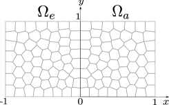
Figure 2: Computational domain and mesh made up by $120$ polygons.

Figure 3 shows convergence results in the dG- and $L^{2}$-norms respectively, for four nested, sequentially refined polygonal meshes, when polynomials of uniform degree $p=2$ are employed. The numerical results concerning the dG-error show asymptotic convergence rates that match those predicted by estimate (42). Also, as it is typical for dG methods, the $L^{2}$-error turns out to converge in $h^{p+1}$ (see, e.g., [65, Theorem 2] for the case of the elastodynamics equation).

Figure 4 shows convergence results in a semilogarithmic scale, in the dG- and $L^{2}$-norms respectively, for a fixed mesh given by 300 elements and a uniform polynomial degree ranging from 1 to 5. Since the exact solution is analytical, as expected, the error undergoes an exponential decay.

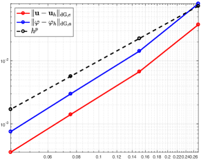
(a) $\|\mathbf{u}-\mathbf{u}_{h}\|_{{\mathrm{dG},e}}$ and $\|\varphi-\varphi_{h}\|_{\mathrm{dG},a}$ vs. $h$ at $T=1$

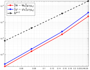
(b) $\|\mathbf{u}-\mathbf{u}_{h}\|_{\Omega_{e}}$ and $\|\varphi-\varphi_{h}\|_{\Omega_{a}}$ vs. $h$ at $T=1$

Figure 3: Test case 1. dG-error and $L^{2}$-error vs. $h$ for four sequentially refined polygonal meshes and second-order polynomials.

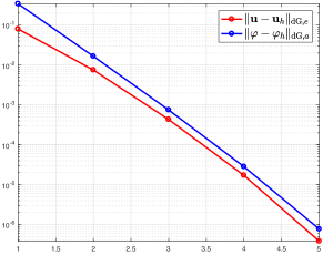
(a) $\|\mathbf{u}-\mathbf{u}_{h}\|_{{\mathrm{dG},e}}$ and $\|\varphi-\varphi_{h}\|_{\mathrm{dG},a}$ vs. $p$ at $T=1$

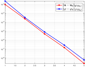
(b) $\|\mathbf{u}-\mathbf{u}_{h}\|_{\Omega_{e}}$ and $\|\varphi-\varphi_{h}\|_{\Omega_{a}}$ vs. $p$ at $T=1$

Figure 4: Test case1. dG-error and $L^{2}$-error vs. $p$ for $p$ ranging from 1 to 5 and a mesh given by 300 polygons.

7.2 Test case 2

We now choose the right-hand sides $\mathbf{f}_{e}$ and $f_{a}$ so that the exact solution is given by

$$\mathbf{u}(x,y;t)=\left(\cos\Big{(}\frac{4\pi x}{c_{p}}\Big{)},\,\cos\Big{(}\frac{4\pi x}{c_{s}}\Big{)}\right)\cos(4\pi t),\ \ \varphi(x,y;t)=\sin(4\pi x)\sin(4\pi t),$$ (68)

where $c_{p}=\sqrt{\frac{\lambda+2\mu}{\rho_{e}}}$ and $c_{s}=\sqrt{\frac{\mu}{\rho_{e}}}$ are the velocities of pressure and shear waves in the elastic domain, respectively. The same test has been carried out in [6] using a Spectral Element discretization; the choice of material parameters is also the same as in the previous test case. In this case, on $\Gamma_{\mathrm{I}}$, both the traction $\bm{\sigma}(\mathbf{u})\mathbf{n}_{e}$ and the acoustic pressure $-\rho_{a}\accentset{\mbox{\footnotesize.}}{\varphi}\mathbf{n}_{e}$ vanish; on the other hand, we have $\partial\varphi/\partial\mathbf{n}_{a}=-\accentset{\mbox{\footnotesize.}}{\mathbf{u}}\cdot\mathbf{n}_{a}=4\pi\sin(4\pi t)$. The timestep is, again, set to $\Delta t=10^{-4}$; on the other hand, the final time is in this case set to $T=0.8$, to ensure that none of the two unknowns $\mathbf{u}$ and $\varphi$ be identically zero when dG- and $L^{2}$-errors are computed.

Figure 5 shows convergence results in the dG- and $L^{2}$-norms respectively, for four nested, sequentially refined polygonal meshes, when polynomials of uniform degree $p=2$ are employed. The numerical results concerning the dG-error again show asymptotic convergence rates matching those predicted by estimate (42). Also, the $L^{2}$-error convergence rates turn out to be slightly higher than $h^{p+1}$ both for $\mathbf{u}$ and for $\varphi$; in the latter case, this difference is more remarkable.

Figures 6 shows convergence results in a semilogarithmic scale, in the dG- and $L^{2}$-norms respectively, for a fixed mesh given by 300 elements and a uniform polynomial degree ranging from 1 to 5. Again, the error undergoes an exponential decay. Notice that, concerning the $L^{2}$-error on $\mathbf{u}$ (Figure 6b), the convergence rate decreases when passing from polynomial degree 4 to 5: in both cases the $L^{2}$-error is on the order of $10^{-7}$. This behavior is related to the choice of the timestep $\Delta t$, set to $10^{-4}$; indeed, when a leap-frog time discretization is employed, the error is expected to converge in $\Delta t^{2}$. In our case, $\Delta t^{2}=10^{-8}$, which is only one order of magnitude lower than the $L^{2}$-error for $p=4$ and $p=5$. Decreasing the timestep to $\Delta t=10^{-5}$ allows to recover the expected convergence.

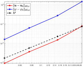
(a) $\|\mathbf{u}-\mathbf{u}_{h}\|_{{\mathrm{dG},e}}$ and $\|\varphi-\varphi_{h}\|_{\mathrm{dG},a}$ vs. $h$ at $T=0.8$

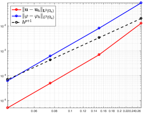
(b) $\|\mathbf{u}-\mathbf{u}_{h}\|_{{\Omega_{e}}}$ and $\|\varphi-\varphi_{h}\|_{{\Omega_{a}}}$ vs. $h$ at $T=0.8$

Figure 5: Test case 2. dG-error and $L^{2}$-error vs. $h$ for four sequentially refined polygonal meshes and second-order polynomials.

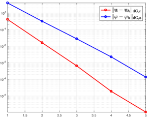
(a) $\|\mathbf{u}-\mathbf{u}_{h}\|_{{\mathrm{dG},e}}$ and $\|\varphi-\varphi_{h}\|_{\mathrm{dG},a}$ vs. $p$ at $T=0.8$

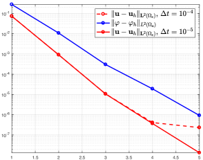
(b) $\|\mathbf{u}-\mathbf{u}_{h}\|_{{\Omega_{e}}}$ and $\|\varphi-\varphi_{h}\|_{{\Omega_{a}}}$ vs. $p$ at $T=0.8$

Figure 6: Test case 2. dG-error and $L^{2}$-error vs. $p$ for $p$ ranging from 1 to 5 and a mesh given by 300 polygons.

7.3 Test case 3: a physical example

As a further numerical experiment, we simulate a seismic source. In particular, we suppose that the system is excited only by a Ricker wavelet, i.e., by the following point source load placed in the acoustic domain:

$$f_{a}(\mathbf{x},t)=-2\pi a\left(1-2\pi a(t-t_{0})^{2}\right)e^{-\pi a(t-t_{0})^{2}}\delta(\mathbf{x}-\mathbf{x}_{0}),\ \ \mathbf{x}_{0}\in{\Omega_{a}},\ t_{0}\in(0,T],$$ (69)

where $\mathbf{x}\equiv(x,y)$, $\mathbf{x}_{0}\equiv(x_{0},y_{0})$ is a given point in ${\Omega_{a}}$, and $\delta$ is the Dirac distribution (cf. Figure 7 for a representation of the time factor in (69)). All initial conditions, as well as the body force $\mathbf{f}_{e}$, are set to zero. The Dirac distribution in $\mathbf{x}_{0}$ is approximated numerically by a Gaussian distribution centered at $\mathbf{x}_{0}$. We consider the following values of the material parameters: $\rho_{e}=2.5$, $\rho_{a}=1$, $\mu=10$, $\lambda=20$, $c=1.5$; also, in (69), we choose $\mathbf{x}_{0}=(0.2,0.5)$, $t_{0}=0.1$, and $a=576$. We employ here a polygonal mesh of 5000 elements, corresponding to a meshsize $h\simeq 0.04$, a uniform polynomial degree $p=3$, and a timestep $\Delta t=10^{-5}$. The final time is set to $T=1$.

Figure 8 shows the numerical solution (horizontal and vertical elastic displacements, and acoustic potential) at time $t=0.5$. The vertical displacement, displayed in Figure 8b, turns out to be very close to zero in a large elastic subregion, except near the boundary, where small reflected wavefronts can be detected, because of homogeneous Dirichlet boundary conditions. This behavior is due to the fact that the seismic source is placed close enough to the interface $\Gamma_{\mathrm{I}}$, so that the effects of reflected waves in the elastic region are not observed for a certain time, and hence only the coupling effects are visible (only longitudinal stresses are propagated through the elasto-acoustic interface, since fluids cannot sustain shear stresses). Nevertheless, after a certain time, elastic waves are reflected, which gives rise to a nonzero vertical displacement. Concerning the acoustic region, spherical wavefronts generated by the point source load can be clearly observed in Figure 8c; again, waves are reflected on the boundary for the same reason as before.

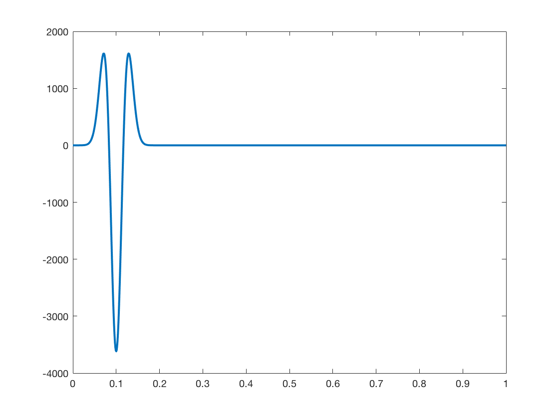
Figure 7: $t\mapsto-2\pi a\left(1-2\pi a(t-t_{0})^{2}\right)e^{-\pi a(t-t_{0})^{2}}$ for $a=576$ and $t_{0}=0.1$.

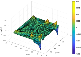
(a) Horizontal elastic displacement at $t=0.5$

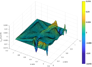
(b) Vertical elastic displacement at $t=0.5$

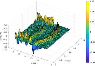
(c) Acoustic potential at $t=0.5$

Figure 8: Numerical solution at $t=0.5$.

Appendix A

Lemma A1.

The following inequalities hold:

$$\|\eta^{-\nicefrac{{1}}{{2}}}{\{\{{\bm{\sigma}_{h}(\mathbf{v})}\}\}}\|_{{\mathcal{F}}_{h}^{e}} \lesssim\frac{1}{\sqrt{\alpha}}\|\mathbb{C}^{\nicefrac{{1}}{{2}}}\bm{\varepsilon}_{h}(\mathbf{v})\|_{\Omega_{e}} \forall\mathbf{v}\in\mathbf{V}_{\!h}^{e},$$ (70a)

$$\|\chi^{-\nicefrac{{1}}{{2}}}{\{\{{\rho_{a}\mathbf{\nabla}_{h}\psi}\}\}}\|_{{\mathcal{F}}_{h}^{a}} \lesssim\frac{1}{\sqrt{\beta}}\|\rho_{a}^{\nicefrac{{1}}{{2}}}\mathbf{\nabla}_{h}\psi\|_{\Omega_{a}} \forall\psi\in V_{h}^{a},$$ (70b)

where $\alpha$ and $\beta$ are the stability parameters appearing in the definition of stabilization functions (22a)–(22b).

Proof.

We only prove (70a), the arguments for showing (70b) being completely analogous.

Recall that the following trace-inverse inequality holds for simplices [16, p. 25]: given a simplex $T\subset\mathbb{R}^{d}$ and a polynomial degree $p\geq 1$, for all $v\in\mathscr{P}_{p}(T)$ there is a real number $C>0$ independent of the discretization parameters such that

$$\|v\|_{F}^{2}\leq Cp^{2}\frac{|F|}{|T|}\|v\|_{T}^{2}.$$ (71)

Owing to (71), the definition (12) of $\overline{\mathbb{C}}_{\kappa}$, the definition (22a) of $\eta$, and Assumption 1a, for any $\mathbf{v}\in\mathbf{V}_{\!h}^{e}$ we obtain

$$\|\eta^{-\nicefrac{{1}}{{2}}}{\{\{{\bm{\sigma}_{h}(\mathbf{v})}\}\}}\|_{{\mathcal{F}}_{h}^{e}}^{2} \leq\sum_{\kappa\in\mathcal{T}_{h}^{e}}\sum_{F\subset\partial\kappa}\overline{\mathbb{C}}_{\kappa}\|\eta^{-\nicefrac{{1}}{{2}}}\mathbb{C}^{\nicefrac{{1}}{{2}}}\bm{\varepsilon}(\mathbf{v})\|_{F}^{2}$$

$$\lesssim\sum_{\kappa\in\mathcal{T}_{h}^{e}}\sum_{F\subset\partial\kappa}\eta^{-1}\overline{\mathbb{C}}_{\kappa}p_{e,\kappa}^{2}\frac{|F|}{|\kappa_{\flat}^{F}|}\|\mathbb{C}^{\nicefrac{{1}}{{2}}}\bm{\varepsilon}(\mathbf{v})\|_{\kappa_{\flat}^{F}}^{2}\lesssim\frac{1}{\alpha}\|\mathbb{C}^{\nicefrac{{1}}{{2}}}\bm{\varepsilon}_{h}(\mathbf{v})\|_{{\Omega_{e}}}^{2}.$$

∎

Lemma A2.

For any ${\mathbf{W}}=(\mathbf{v},\psi)\in C^{1}([0,T];\mathbf{V}_{\!h}^{e})\times C^{1}([0,T];V_{h}^{a})$, it holds

$$\|{\mathbf{W}}\|_{\mathcal{E}}^{2}-2\left(\left\langle{\{\{{\bm{\sigma}_{h}(\mathbf{v})}\}\}},{[[{\mathbf{v}}]]}\right\rangle_{{\mathcal{F}}_{h}^{e}}+\left\langle{\{\{{\rho_{a}\mathbf{\nabla}_{h}\psi}\}\}},{[[{\psi}]]}\right\rangle_{{\mathcal{F}}_{h}^{a}}\right) \lesssim\|{\mathbf{W}}\|_{\mathcal{E}}^{2},$$ (72)

$$\|{\mathbf{W}}\|_{\mathcal{E}}^{2}-2\left(\left\langle{\{\{{\bm{\sigma}_{h}(\mathbf{v})}\}\}},{[[{\mathbf{v}}]]}\right\rangle_{{\mathcal{F}}_{h}^{e}}+\left\langle{\{\{{\rho_{a}\mathbf{\nabla}_{h}\psi}\}\}},{[[{\psi}]]}\right\rangle_{{\mathcal{F}}_{h}^{a}}\right) \gtrsim\|{\mathbf{W}}\|_{\mathcal{E}}^{2},$$

Proof.

The first bound follows from the Cauchy–Schwarz inequality, the definition (26) of the energy norm, and Lemma A1:

$$\|{\mathbf{W}}\|_{\mathcal{E}}^{2}\ - \ 2\left(\left\langle{\{\{{\bm{\sigma}_{h}(\mathbf{v})}\}\}},{[[{\mathbf{v}}]]}\right\rangle_{{\mathcal{F}}_{h}^{e}}+\left\langle{\{\{{\rho_{a}\mathbf{\nabla}_{h}\psi}\}\}},{[[{\psi}]]}\right\rangle_{{\mathcal{F}}_{h}^{a}}\right)$$

$$\lesssim\ \|{\mathbf{W}}\|_{\mathcal{E}}^{2}+\|\eta^{-\nicefrac{{1}}{{2}}}{\{\{{\bm{\sigma}_{h}(\mathbf{v})}\}\}}\|_{{\mathcal{F}}_{h}^{e}}\|\eta^{\nicefrac{{1}}{{2}}}{[[{\mathbf{v}}]]}\|_{{\mathcal{F}}_{h}^{e}}+\|\chi^{-\nicefrac{{1}}{{2}}}{\{\{{\rho_{a}\mathbf{\nabla}_{h}\psi}\}\}}\|_{{\mathcal{F}}_{h}^{a}}\|\chi^{\nicefrac{{1}}{{2}}}{[[{\psi}]]}\|_{{\mathcal{F}}_{h}^{a}}$$

$$\lesssim\|{\mathbf{W}}\|_{\mathcal{E}}^{2}+\frac{1}{\sqrt{\alpha}}\|\mathbb{C}^{\nicefrac{{1}}{{2}}}\bm{\varepsilon}_{h}(\mathbf{v})\|_{\Omega_{e}}\|\mathbf{v}\|_{\mathrm{dG},e}+\frac{1}{\sqrt{\beta}}\|\rho_{a}^{\nicefrac{{1}}{{2}}}\mathbf{\nabla}_{h}\psi\|_{\Omega_{a}}\|\psi\|_{\mathrm{dG},a}$$

$$\lesssim\|{\mathbf{W}}\|_{\mathcal{E}}^{2}+\|{\mathbf{W}}\|_{\mathrm{dG}}^{2}\lesssim\|{\mathbf{W}}\|_{\mathcal{E}}^{2},$$

where we have set $\|{\mathbf{W}}\|_{\mathrm{dG}}^{2}=\|\mathbf{v}\|_{{\mathrm{dG}},e}^{2}+\|\psi\|_{{\mathrm{dG}},a}^{2}$. To prove the second bound, it suffices to show that

$$\|{\mathbf{W}}\|_{\mathrm{dG}}^{2}-2\left(\left\langle{\{\{{\bm{\sigma}_{h}(\mathbf{v})}\}\}},{[[{\mathbf{v}}]]}\right\rangle_{{\mathcal{F}}_{h}^{e}}+\left\langle{\{\{{\rho_{a}\mathbf{\nabla}_{h}\psi}\}\}},{[[{\psi}]]}\right\rangle_{{\mathcal{F}}_{h}^{a}}\right)\gtrsim\|{\mathbf{W}}\|_{\mathrm{dG}}^{2}.$$ (73)

Indeed, by the definition (26) of the energy norm and (73),

$$\|{\mathbf{W}}\|_{\mathcal{E}}^{2}-2\left(\left\langle{\{\{{\bm{\sigma}_{h}(\mathbf{v})}\}\}},{[[{\mathbf{v}}]]}\right\rangle_{{\mathcal{F}}_{h}^{e}}+\left\langle{\{\{{\rho_{a}\mathbf{\nabla}_{h}\psi}\}\}},{[[{\psi}]]}\right\rangle_{{\mathcal{F}}_{h}^{a}}\right)\\ =\|\rho_{e}^{\nicefrac{{1}}{{2}}}\accentset{\mbox{\footnotesize.}}{\mathbf{v}}\|_{\Omega_{e}}^{2}+\|\rho_{e}^{\nicefrac{{1}}{{2}}}\zeta\mathbf{v}\|_{\Omega_{e}}^{2}+\|c^{-1}\rho_{a}^{\nicefrac{{1}}{{2}}}\accentset{\mbox{\footnotesize.}}{\psi}\|_{\Omega_{a}}^{2}+\|{\mathbf{W}}\|_{\mathrm{dG}}^{2}-2\left(\left\langle{\{\{{\bm{\sigma}_{h}(\mathbf{v})}\}\}},{[[{\mathbf{v}}]]}\right\rangle_{{\mathcal{F}}_{h}^{e}}+\left\langle{\{\{{\rho_{a}\mathbf{\nabla}_{h}\psi}\}\}},{[[{\psi}]]}\right\rangle_{{\mathcal{F}}_{h}^{a}}\right)\\ \gtrsim\|\rho_{e}^{\nicefrac{{1}}{{2}}}\accentset{\mbox{\footnotesize.}}{\mathbf{v}}\|_{\Omega_{e}}^{2}+\|\rho_{e}^{\nicefrac{{1}}{{2}}}\zeta\mathbf{v}\|_{\Omega_{e}}^{2}+\|c^{-1}\rho_{a}^{\nicefrac{{1}}{{2}}}\accentset{\mbox{\footnotesize.}}{\psi}\|_{\Omega_{a}}^{2}+\|{\mathbf{W}}\|_{\mathrm{dG}}^{2}=\|{\mathbf{W}}\|_{\mathcal{E}}^{2}.$$

Thus, we next show that (73) holds provided the stability parameters $\alpha$ and $\beta$ are chosen large enough. To this purpose, using Young’s inequality we infer that, for any $\delta,\epsilon>0$,

$$\left\langle{\{\{{\bm{\sigma}_{h}(\mathbf{v})}\}\}},{[[{\mathbf{v}}]]}\right\rangle_{{\mathcal{F}}_{h}^{e}} \leq\sum_{F\in{\mathcal{F}}_{h}^{e}}\|\eta^{-\nicefrac{{1}}{{2}}}{\{\{{\bm{\sigma}_{h}(\mathbf{v})}\}\}}\|_{F}\|\eta^{\nicefrac{{1}}{{2}}}{[[{\mathbf{v}}]]}\|_{F}\leq\frac{1}{2\delta}\|\eta^{-\nicefrac{{1}}{{2}}}{\{\{{\bm{\sigma}_{h}(\mathbf{v})}\}\}}\|_{{\mathcal{F}}_{h}^{e}}^{2}+\frac{\delta}{2}\|\eta^{\nicefrac{{1}}{{2}}}{[[{\mathbf{v}}]]}\|_{{\mathcal{F}}_{h}^{e}}^{2},$$

$$\left\langle{\{\{{\rho_{a}\mathbf{\nabla}_{h}\psi}\}\}},{[[{\psi}]]}\right\rangle_{{\mathcal{F}}_{h}^{a}} \leq\sum_{F\in{\mathcal{F}}_{h}^{a}}\|\chi^{-\nicefrac{{1}}{{2}}}{\{\{{\rho_{a}\mathbf{\nabla}_{h}\psi}\}\}}\|_{F}\|\chi^{\nicefrac{{1}}{{2}}}{[[{\psi}]]}\|_{F}\leq\frac{1}{2\epsilon}\|\chi^{-\nicefrac{{1}}{{2}}}{\{\{{\rho_{a}\mathbf{\nabla}_{h}\psi}\}\}}\|_{{\mathcal{F}}_{h}^{a}}^{2}+\frac{\epsilon}{2}\|\chi^{\nicefrac{{1}}{{2}}}{[[{\psi}]]}\|_{{\mathcal{F}}_{h}^{a}}^{2}.$$

Hence, from the definition of the $\|{\cdot}\|_{{\mathrm{dG}},e}$- and $\|{\cdot}\|_{{\mathrm{dG}},a}$-norms on $\mathbf{V}_{\!h}^{e}$ and $V_{h}^{a}$, it follows that

$$\|{\mathbf{W}}\|_{\mathrm{dG}}^{2}-2\left(\left\langle{\{\{{\bm{\sigma}_{h}(\mathbf{v})}\}\}},{[[{\mathbf{v}}]]}\right\rangle_{{\mathcal{F}}_{h}^{e}}+\left\langle{\{\{{\rho_{a}\mathbf{\nabla}_{h}\psi}\}\}},{[[{\psi}]]}\right\rangle_{{\mathcal{F}}_{h}^{a}}\right)\\ \geq\|\mathbb{C}^{\nicefrac{{1}}{{2}}}\bm{\varepsilon}(\mathbf{v})\|_{\Omega_{e}}^{2}+\|\rho_{a}^{\nicefrac{{1}}{{2}}}\mathbf{\nabla}_{h}\psi\|_{\Omega_{a}}^{2}+\left(1-{\delta}\right)\|\eta^{\nicefrac{{1}}{{2}}}{[[{\mathbf{v}}]]}\|_{{\mathcal{F}}_{h}^{e}}^{2}-\frac{1}{\delta}\|\eta^{-\nicefrac{{1}}{{2}}}{\{\{{\bm{\sigma}_{h}(\mathbf{v})}\}\}}\|_{{\mathcal{F}}_{h}^{e}}^{2}\\ +\left(1-{\epsilon}\right)\|\chi^{\nicefrac{{1}}{{2}}}{[[{\psi}]]}\|_{{\mathcal{F}}_{h}^{a}}^{2}-\frac{1}{\epsilon}\|\chi^{-\nicefrac{{1}}{{2}}}{\{\{{\rho_{a}\mathbf{\nabla}_{h}\psi}\}\}}\|_{{\mathcal{F}}_{h}^{a}}^{2}\\ \geq\left(1-\frac{C_{1}}{\alpha\delta}\right)\|\mathbb{C}^{\nicefrac{{1}}{{2}}}\bm{\varepsilon}_{h}(\mathbf{v})\|_{\Omega_{e}}^{2}+\left(1-\frac{C_{2}}{\beta\epsilon}\right)\|\rho_{a}^{\nicefrac{{1}}{{2}}}\mathbf{\nabla}_{h}\psi\|_{\Omega_{a}}^{2}\\ +\left(1-{\delta}\right)\|\eta^{\nicefrac{{1}}{{2}}}{[[{\mathbf{v}}]]}\|_{{\mathcal{F}}_{h}^{e}}^{2}+\left(1-{\epsilon}\right)\|\chi^{\nicefrac{{1}}{{2}}}{[[{\psi}]]}\|_{{\mathcal{F}}_{h}^{a}}^{2},$$

where in the last bound we have applied Lemma A1 with hidden constants $C_{1}$ and $C_{2}$. Then (73) follows by choosing, for instance, $\delta=\epsilon=\nicefrac{{1}}{{2}}$ and $\alpha\geq 4C_{1}$, $\beta\geq 4C_{2}$. ∎

References

- [1] D. N. Arnold, F. Brezzi, B. Cockburn, L. D. Marini, Unified analysis of discontinuous Galerkin methods for elliptic problems, SIAM J. Numer. Anal. 39 (2002) 1749–1779.
- [2] B. Rivière, Discontinuous Galerkin methods for solving elliptic and parabolic equations, Frontiers in Applied Mathematics, SIAM, 2008.
- [3] D. A. Di Pietro, A. Ern, Mathematical aspects of Discontinuous Galerkin methods, Mathématiques & Applications, Springer-Verlag, 2012.
- [4] J. S. Hesthaven, T. Warburton, Nodal Discontinuous Galerkin Methods, Vol. 54 of Texts in Applied Mathematics, Springer-Verlag New York, 2008.
- [5] B. Flemisch, M. Kaltenbacher, B. I. Wohlmuth, Elasto–acoustic and acoustic–acoustic coupling on non-matching grids, Int. J. Numer. Meth. Engng 67 (2006) 1791–1810.
- [6] S. Mönköla, Numerical simulation of fluid-structure interaction between acoustic and elastic waves, Ph.D. thesis, University of Jyväskylä (2011).
- [7] P. F. Antonietti, P. Houston, X. Hu, M. Sarti, M. Verani, Multigrid algorithms for hp-version interior penalty discontinuous Galerkin methods on polygonal and polyhedral meshes, Calcolo 54 (2017) 1169–1198.
- [8] P. F. Antonietti, A. Cangiani, J. Collis, Z. Dong, E. H. Georgoulis, S. Giani, P. Houston, Review of discontinuous galerkin finite element methods for partial differential equations on complicated domains, in: G. Barrenechea, F. Brezzi, A. Cangiani, E. Georgoulis (Eds.), Building bridges: connections and challenges in modern approaches to numerical partial differential equations, Vol. 114 of Lecture Notes in Computational Science and Engineering, Springer, Cham, 2016.
- [9] P. F. Antonietti, I. Mazzieri, High-order discontinuous Galerkin methods for the elastodynamics equation on polygonal and polyhedral meshes, MOX-Report No. 06/2018, submitted (2018).
- [10] P. F. Antonietti, F. Brezzi, L. D. Marini, Bubble stabilization of discontinuous Galerkin methods, Comput. Methods Appl. Mech. Engrg. 198 (2009) 1651–1659.
- [11] A. Cangiani, E. H. Georgoulis, P. Houston, -Version discontinuous Galerkin methods on polygonal and polyhedral meshes, Math. Models Methods Appl. Sci. 24 (2014) 2009–2041.
- [12] A. Cangiani, Z. Dong, E. H. Georgoulis, P. Houston, -Version discontinuous Galerkin methods for advection–diffusion–reaction problems on polytopic meshes, ESAIM Math. Model. Numer. Anal. 50 (2016) 699–725.
- [13] A. Cangiani, Z. Dong, E. H. Georgoulis, -Version space-time discontinuous Galerkin methods for parabolic problems on prismatic meshes, SIAM J. Sci. Comput. 39 (2017) A1251–A1279.
- [14] P. F. Antonietti, G. Pennesi, -cycle multigrid algorithms for discontinuous Galerkin methods on non-nested polytopic meshes, J. Sci. Comput. Published online. doi:10.1007/s10915-018-0783-x.
- [15] P. F. Antonietti, P. Houston, G. Pennesi, Fast numerical integration on polytopic meshes with applications to discontinuous Galerkin finite element methods, J. Sci. Comput. 77 (2018) 1339–1370.
- [16] A. Cangiani, Z. Dong, E. H. Georgoulis, P. Houston, -Version discontinuous Galerkin methods on polygonal and polyhedral meshes, SpringerBriefs in Mathematics, Springer International Publishing, 2017.
- [17] N. Sukumar, A. Tabarrei, Conforming polygonal finite elements, Int. J. Numer. Meth. Engng 61 (2004) 2045–2066.
- [18] A. Tabarrei, N. Sukumar, Application of polygonal finite elements in linear elasticity, Int. J. Comput. Methods 3 (2006) 503–520.
- [19] G. Manzini, A. Russo, N. Sukumar, New perspectives on polygonal and polyhedral finite element methods, Math. Models Methods Appl. Sci. 24 (2014) 1665–1699.
- [20] A. Tabarrei, N. Sukumar, Extended finite-element method on polygonal and quadtree meshes, Comput. Methods Appl. Mech. Engrg. 197 (2008) 425–438.
- [21] P. F. Antonietti, N. Bigoni, M. Verani, Mimetic discretizations of elliptic control problems, J. Sci. Comput. 56 (2013) 14–27.
- [22] F. Brezzi, A. Buffa, K. Lipnikov, Mimetic finite differences for elliptic problems, ESAIM Math. Model. Numer. Anal. 43 (2009) 277–295.
- [23] V. Gyrya, K. Lipnikov, G. Manzini, The arbitrary order mixed mimetic finite difference method for the diffusion equation, ESAIM Math. Model. Numer. Anal. 50 (2016) 851–877.
- [24] L. Beirão da Veiga, K. Lipnikov, G. Manzini, Arbitrary-order nodal mimetic discretizations of elliptic problems on polygonal meshes, SIAM J. Numer. Anal. 49 (2011) 1737–1760.
- [25] L. Beirão da Veiga, F. Brezzi, L. D. Marini, A. Russo, Basic principles of virtual element methods, Math. Models Methods Appl. Sci. 23 (2013) 199–214.
- [26] L. Beirão da Veiga, F. Brezzi, L. D. Marini, A. Russo, Mixed virtual element methods for general second order elliptic problems on polygonal meshes, ESAIM Math. Model. Numer. Anal. 50 (2016) 727–747.
- [27] L. Beirão da Veiga, F. Brezzi, L. D. Marini, A. Russo, Virtual element method for general second-order elliptic problems on polygonal meshes, Math. Models Methods Appl. Sci. 26 (2016) 729–750.
- [28] P. F. Antonietti, G. Manzini, M. Verani, The fully nonconforming virtual element method for biharmonic problems, Math. Models Methods Appl. Sci. 28 (2018) 387–407.
- [29] B. Cockburn, J. Gopalakrishnan, R. Lazarov, Unified hybridization of discontinuous Galerkin, mixed, and continuous Galerkin methods for second order elliptic problems, SIAM J. Numer. Anal. 47 (2009) 1319–1365.
- [30] R. M. Kirby, S. J. Sherwin, B. Cockburn, To CG or to HDG: a comparative study, J. Sci. Comput. 51 (2012) 183–212.
- [31] B. Cockburn, J. Gopalakrishnan, F. J. Sayas, A projection-based error analysis of hdg methods, Math. Comp. 79 (2010) 1351–1367.
- [32] B. Cockburn, M. Solano, Solving dirichlet boundary-value problems on curved domains by extensions from subdomains, SIAM J. Sci. Comput. 34 (2012) A497–A519.
- [33] B. Cockburn, O. Dubois, J. Gopalakrishnan, S. Tan, Multigrid for an hdg method, IMA J. Numer. Anal. 34 (2014) 1386–1425.
- [34] D. A. Di Pietro, A. Ern, A hybrid high-order locking-free method for linear elasticity on general meshes, Comput. Methods Appl. Mech. Engrg. 283 (2015) 1–21.
- [35] D. A. Di Pietro, A. Ern, S. Lemaire, An arbitrary-order and compact-stencil discretization of diffusion on general meshes based on local reconstruction operators, Comput. Method Appl. Math. 14 (2014) 461–472.
- [36] D. A. Di Pietro, J. Droniou, A hybrid high-order method for Leray–Lions elliptic equations on general meshes, Math. Comp. 86 (2017) 2159–2191.
- [37] F. Bonaldi, D. A. Di Pietro, G. Geymonat, F. Krasucki, A hybrid high-order method for Kirchhoff–Love plate bending problems, ESAIM Math. Model. Numer. Anal. 52 (2018) 393–421.
- [38] D. A. Di Pietro, R. Tittarelli, An introduction to hybrid high-order methods, in: D. A. Di Pietro, A. Ern, L. Formaggia (Eds.), Lectures from the Fall 2016 thematic quarter at Institut Henri Poincaré, Springer, 2017, accepted for publication.
- [39] A. Bermúdez, L. Hervella-Nieto, R. Rodríguez, Finite element computation of three-dimensional elastoacoustic vibrations, Journal of Sound and Vibration 219 (1999) 279–306.
- [40] H. Barucq, R. Djellouli, E. Estecahandy, Characterization of the Fréchet derivative of the elasto-acoustic field with respect to Lipschitz domains, J. Inverse Ill-Posed Probl. 22 (2014) 1–8.
- [41] H. Barucq, R. Djellouli, E. Estecahandy, Efficient dg-like formulation equipped with curved boundary edges for solving elasto-acoustic scattering problems, Int. J. Numer. Meth. Engng 98 (2014) 747–780.
- [42] D. Brunner, M. Junge, L. Gaul, A comparison of FE–BE coupling schemes for large-scale problems with fluid-structure interaction, Int. J. Numer. Meth. Engng 77 (2009) 664–688.
- [43] J. D. De Basabe, M. K. Sen, A comparison of finite-difference and spectral-element methods for elastic wave propagation in media with a fluid-solid interface, Geophysical Journal International 200 (2015) 278–298.
- [44] M. Fischer, L. Gaul, Fast BEM–FEM mortar coupling for acoustic-structure interaction, Int. J. Numer. Meth. Engng 62 (2005) 1677–1690.
- [45] J. Mandel, An iterative substructuring method for coupled fluid–solid acoustic problems, J. Comput. Phys. 177 (2002) 95–116.
- [46] S. Mönköla, On the accuracy and efficiency of transient spectral element models for seismic wave problems, Adv. Math. Phys.
- [47] V. Péron, Equivalent boundary conditions for an elasto-acoustic problem set in a domain with a thin layer, ESAIM Math. Model. Numer. Anal. 48 (2014) 1431–1449.
- [48] M. Popa, Finite element solution of scattering in coupled fluid-solid systems, Ph.D. thesis, University of Colorado (2002).
- [49] G. W. Benthien, H. A. Schenck, Structural-acoustic coupling, in: R. Ciskowski, C. Brebbia (Eds.), Boundary element methods in acoustics, Computational mechanics publications, Elsevier Applied Science, Southampton, 1991.
- [50] B. Flemisch, M. Kaltenbacher, S. Triebenbacher, B. I. Wohlmuth, The equivalence of standard and mixed finite element methods in applications to elasto-acoustic interaction, SIAM J. Sci. Comput. 32 (2010) 1980–2006.
- [51] G. C. Hsiao, N. Nigam, A transmission problem for fluid-structure interaction in the exterior of a thin domain, Adv. Differential Equations 8 (2003) 1281–1318.
- [52] G. C. Hsiao, F. J. Sayas, R. J. Weinacht, Time-dependent fluid-structure interaction, Math. Methods Appl. Sci. 40 (2017) 486–500.
- [53] G. C. Hsiao, T. Sánchez-Vizuet, F. J. Sayas, Boundary and coupled boundary–finite element methods for transient wave–structure interaction, IMA J. Numer. Anal. 37 (2017) 237–265.
- [54] R. A. Jeans, I. C. Mathews, Solution of fluid-structure interaction problems using a coupled finite element and variational boundary element technique, The Journal of the Acoustical Society of America 88.
- [55] D. Komatitsch, C. Barnes, J. Tromp, Wave propagation near a fluid-solid interface: a spectral-element approach, Geophysics 65 (2000) 623–631.
- [56] H. Y. Lee, S. C. Lim, D. J. Min, B. D. Kwon, M. Park, 2D time-domain acoustic-elastic coupled modeling: a cell-based finite-difference method, Geosciences Journal 13 (2009) 407–414.
- [57] H. Brezis, Functional analysis, Sobolev spaces and partial differential equations, Universitext, Springer-Verlag New York, 2011.
- [58] T. S. Brown, T. Sánchez-Vizuet, F. J. Sayas, Evolution of a semidiscrete system modeling the scattering of acoustic waves by a piezoelectric solid, ESAIM Math. Model. Numer. Anal. 52 (2018) 423–455.
- [59] R. Kosloff, D. Kosloff, Absorbing boundaries for wave propagation problems, J. Comput. Phys. 63 (1986) 363–376.
- [60] F. Bonaldi, G. Geymonat, F. Krasucki, Modeling of smart materials with thermal effects: dynamic and quasi-static evolution, Math. Models Methods Appl. Sci. 25 (2015) 2633–2667.
- [61] I. Perugia, D. Schötzau, An -analysis of the local discontinuous galerkin method for diffusion problems, J. Sci. Comput. 17 (2002) 561–571.
- [62] P. F. Antonietti, A. Ferroni, I. Mazzieri, R. Paolucci, A. Quarteroni, C. Smerzini, M. Stupazzini, Numerical modeling of seismic waves by discontinuous spectral element methods, ESAIM:ProcS.
- [63] D. N. Arnold, F. Brezzi, R. S. Falk, L. D. Marini, Locking-free Reissner–Mindlin elements without reduced integration, Comput. Methods Appl. Mech. Engrg. 196 (2007) 3660–3671.
- [64] P. F. Antonietti, B. Ayuso de Dios, I. Mazzieri, A. Quarteroni, Stability analysis of discontinuous Galerkin approximations to the elastodynamics problem, J. Sci. Comput. 68 (2016) 143–170.
- [65] P. F. Antonietti, A. Ferroni, I. Mazzieri, A. Quarteroni, -Version discontinuous Galerkin approximations of the elastodynamics equation, in: M. Bittencourt, N. Dumont, J. Hesthaven (Eds.), Spectral and High Order Methods for Partial Differential Equations ICOSAHOM 2016, Vol. 119 of Lecture Notes in Computational Science and Engineering, Springer, Cham, 2017.
- [66] A. Quarteroni, Numerical Models for Differential Problems, 2nd Edition, Vol. 8 of MS&A, Springer-Verlag Mailand, 2014.
- [67] A. Quarteroni, A. Valli, Numerical Approximation of Partial Differential Equations, Vol. 23, Springer Science & Business Media, 2008.
- [68] C. Talischi, G. H. Paulino, A. Pereira, I. F. M. Menezes, PolyMesher: a general-purpose mesh generator for polygonal elements written in Matlab, Struct. Multidisc. Optim. 45 (2012) 309–328.