How do hydrogen bonds break in supercooled water?: Detecting pathways not going through saddle point of two-dimensional potential of mean force

Abstract

Supercooled water exhibits remarkably slow dynamics similar to the behavior observed for various glass-forming liquids. The local order of tetrahedral structures due to hydrogen-bonds (H-bonds) increases with decreasing temperature. Thus, it is important to clarify the temperature dependence of the H-bond breakage process. This was investigated here using molecular dynamics simulations of TIP4P supercooled water. The two-dimensional (2D) potential of mean force (PMF) is presented using combinations of intermolecular distance and angle between two water molecules. The saddle point of the 2D PMF suggests the presence of the transition state that distinguishes between H-bond and non H-bond states. However, we observed pathways not going through this saddle point particularly at supercooled states, which are due to translational, rather than rotational motions of the molecules. We quantified the characteristic time scales of rotational and translational H-bond breakages. The time scale of translational H-bond breakage shows a non-Arrhenius temperature dependence comparable to that of the H-bond lifetime. This time scale is relevant for the temperature dependence of the transmission coefficient based on the transition state theory. The translational H-bond breakage is also related to cage-jumps observed in glass-forming liquids, which mostly involve spatially correlated molecules. Our findings warrant further exploration of an appropriate free-energy surface or reaction coordinates beyond the geometrical variables of the water dimer to describe a possible saddle point related to collective jump motions.

I Introduction

Liquid water is a complex material that exhibits many anomalous properties. Eisenberg and Kauzmann (2005) When liquid water is supercooled below its melting temperature, such anomalies become remarkable. The controversial concept of a liquid-liquid transition in deeply supercooled states has attracted much attention from researchers. Debenedetti (2003); Stanley (2013); Gallo et al. (2016) Thus, clarification of the structures and dynamics in supercooled water has been increasingly important in recent years. In particular, water molecules in supercooled water exhibit remarkably slow dynamics similar to that of viscous glass-forming liquids. Gallo et al. (1996); Sciortino et al. (1996, 1997); Giovambattista et al. (2003, 2005); Chen et al. (2006); Kumar et al. (2007); Xu et al. (2009); Gallo and Rovere (2012); Dehaoui, Issenmann, and Caupin (2015); De Marzio et al. (2016); Guillaud et al. (2017); Galamba (2017); De Marzio et al. (2017); Kawasaki and Kim (2017); Singh, Issenmann, and Caupin (2017)

It is generally expected that the hydrogen-bonds (H-bonds) of water molecules play a crucial role in determining their anomalous properties. Eisenberg and Kauzmann (2005) A large number of experiments and simulations have been carried out to investigate the local structure of H-bonds and the network rearrangement. Stillinger (1975, 1980); Ohmine and Tanaka (1993); Teixeira, Luzar, and Longeville (2006); Bakker and Skinner (2010); Agmon (2012); Perakis et al. (2016) The H-bond is generally defined based on certain structural or energetic criteria of the water-water configuration. Various H-bond definitions in liquid water have been developed for molecular dynamics (MD) simulations. Kumar, Schmidt, and Skinner (2007); Matsumoto (2007); Prada-Gracia, Shevchuk, and Rao (2013); Ozkanlar, Zhou, and Clark (2014) A widely used criterion for determining the H-bond is a geometry definition for a pair of water molecules, i.e., a pair of water molecules is considered H-bonded if the intermolecular distance and angle become less than pre-assigned threshold values. Accordingly, the H-bond correlation function is formulated, allowing quantification of the averaged H-bond lifetime, $\tau_{\mathrm{HB}}$. Stillinger (1975); Rapaport (1983); Luzar and Chandler (1996a, b); Luzar (2000) Its derivative with respect to time, which is related to the reactive flux, characterizes the H-bond breakage rate. Luzar and Chandler (1996a, b); Luzar (2000) As an alternative to $\tau_{\mathrm{HB}}$ from the correlation function, the distribution function of the H-bond lifetime has been examined using the trajectory based analyses. Sciortino et al. (1990); Starr, Nielsen, and Stanley (1999, 2000); Henchman and Irudayam (2010); Martiniano and Galamba (2013); Galamba (2017) Furthermore, the molecular mechanism of the breakage and reforming of H-bond was comprehensively investigated considering molecular mobility of bifurcated H-bonds Sciortino, Geiger, and Stanley (1991, 1992) and molecular reorientational motions. Laage and Hynes (2006, 2008); Henchman and Irudayam (2010); Stirnemann and Laage (2012); Henchman (2016).

The analysis of H-bond dynamics was also applied in MD simulations of supercooled water. Starr, Nielsen, and Stanley (1999, 2000); Stirnemann and Laage (2012); Martiniano and Galamba (2013); Saito, Ohmine, and Bagchi (2013); Kawasaki and Kim (2017) The temperature dependence is conventionally analyzed by examining the Arrhenius plot, $\tau_{\mathrm{HB}}\propto\exp(E_{\mathrm{A}}/k_{\mathrm{B}}T)$, where $T$ is the temperature, $k_{\mathrm{B}}$ is the Boltzmann constant, and $E_{\mathrm{A}}$ is the Arrhenius activation energy of H-bond breakage considering reaction rate theory. The MD studies revealed that $\tau_{\mathrm{HB}}$ significantly increased with decreasing temperature, showing non-Arrhenius behavior, where $E_{\mathrm{A}}$ increased with decreasing the temperature. Collective molecular motions are expected to be a possible scenario by using the analogy with dynamic heterogeneities in glassy systems. Berthier et al. (2011) However, generally speaking, it is difficult to interpret for $E_{\mathrm{A}}$ of supercooled liquids and glasses, i.e., a fragility classification for the temperature dependence of the dynamics. Angell (2008) The fragility is also relevant with searching for transition states connecting numerous stable states in the rugged free-energy landscape of complex many-body systems. Stillinger (1995); Debenedetti and Stillinger (2001) A study based on this concept was reported using configuration-space-network analysis for H-bond rearrangements. Prada-Gracia et al. (2012)

Kumar et al. proposed a method to describe the profile for the two-dimensional (2D) potential of mean force (PMF), which is also referred to as the free-energy surface, from the distribution function of the intermolecular distance and angle between two water molecules. Kumar, Schmidt, and Skinner (2007) This 2D PMF profile enabled the systematic quantification of the distance and angle thresholds, which distinguishes between H-bond and non H-bond regions in classical MD simulations. In Ref. Kumar, Schmidt, and Skinner, 2007, an attempt was made to understand the consistency with H-bond definition based on an electronic structure of water dimer. In addition, profiles of 2D PMF have been also provided by recent ab initio MD simulations. Morawietz et al. (2016); Chen et al. (2017) If the chosen intermolecular distance and angle are treated as the reaction coordinates for the H-bond breakage transition, the dynamics of H-bond breakage is then predicted by the pathway that goes through the saddle point on the 2D PMF profile.

In general, it is challenging to appropriately describe the transition state in various chemical processes in many-body systems, including the H-bond breakage in liquid water investigated here. Bolhuis, Dellago, and Chandler (1998); Geissler, Dellago, and Chandler (1999); Bolhuis, Dellago, and Chandler (2000) Using a stochastic transition path sampling method for rare events, the kinetic pathway of the H-bond breakage in liquid water was investigated, but little attention was paid to the connection with the 2D PMF. Csajka and Chandler (1998) The aim of this study is to address the pathway of H-bond breakage, particularly in supercooled water. In addition, we discuss the mechanism of the non-Arrhenius behavior of the temperature dependence of $\tau_{\mathrm{HB}}$.

This study analyses the impact of the the H-bond breakage dynamics in TIP4P supercooled water using MD simulations. The investigated temperatures ranged from 300 K to 190 K at a fixed volume. Using the geometrical variables between water dimer, we calculated the distance-angle distribution function and the associated 2D PMF. Kumar, Schmidt, and Skinner (2007) From the 2D profile, H-bond and non H-bond regions are distinguished by specifying the saddle point. The H-bond lifetime was quantified from the H-bond correlation function. In addition, the transmission coefficient was calculated based on transition state theory (TST) from reactive flux analysis. Chandler (1978); Hänggi, Talkner, and Borkovec (1990) and its relationship with the free-energy barrier of the saddle point on the 2D PMF profile was examined.

The present work also focuses on the characteristic time scales of rotational and translational H-bond breakages, which were evaluated from the time dependent H-bond breakage populations. To this aim, the populations in the neighboring regions of the H-bond region were quantified on the 2D PMF profile. The physical implication of the transmission coefficient was examined considering the relationship between rotational and translational H-bond breakages.

II Model and simulations

MD simulations were performed using the TIP4P water model. Jorgensen et al. (1983) The various properties of this model have been intensely examined so far. In particular, the comparison with other models including TIP4P/2005 was carefully performed. Vega and Abascal (2011) All the simulations in this work were performed with the GROMACS package. Hess et al. (2008); Abraham et al. (2015) The simulation system contained $N=1,000$ molecules in the cubic box with the periodic boundary conditions. The mass density was fixed at $1$ $\mathrm{g/cm^{3}}$. Correspondingly, the linear dimension of the system was approximately 3.1 nm. The investigated temperatures were $T=300$, $260$, $240$, $220$, $210$, $200$, and $190$ K. The system was first equilibrated with the NVT ensemble at each temperature for 10 ns. Then, the trajectories for the calculations of various quantities were produced with the NVE ensemble for 10 ns ($T\geq 210$ K) and 100 ns ($T\leq 200$ K). A time step of 1 fs was used. For this model, dynamical quantities such as intermediate scattering function and mean square displacement have been reported previously, Gallo and Rovere (2012) with which our simulation results were in agreement (data not shown). This indicates that our computational setups are adequate in turn.

The H-bond was investigated by using distance-angle definitions between two water molecules. Kumar, Schmidt, and Skinner (2007) Specifically, a pair of $R$ and $\beta$ was chosen, where $R$ represents the O-O intermolecular distance and $\beta$ is the O-OH intermolecular angle. Note that $0<\beta<180^{\circ}$. The combined distance-angle distribution function, $g(R,\beta)$, was calculated at each temperature. Kumar, Schmidt, and Skinner (2007) For this $R$-$\beta$ definition, $2\pi\rho R^{2}\sin\beta g(R,\beta)dRd\beta$ represents the averaged number of O atoms found in the partial spherical shell having $dR$ and $d\beta$ at distance $R$ and angle $\beta$ from one fixed O atom. Here, $\rho$ is the molecular density of the system. The function $g(R,\beta)$ results in the PMF defined by $W(R,\beta)=-k_{\mathrm{B}}T\ln g(R,\beta)$. This 2D PMF can be regarded as the free-energy surface using reaction coordinates $(R,\beta)$. The saddle point of $W(R,\beta)$ was numerically determined from the calculations of the gradient $\nabla W(R,\beta)$. Furthermore, the free-energy difference $\Delta G^{\ddagger}$ between the global minimum and saddle point was quantified.

We calculated the time correlation function of the H-bond, $c(t)=\langle h(0)h(t)\rangle/\langle h(0)\rangle,$ where $h(t)$ denotes the H-bond operator at a time $t$. Luzar and Chandler (1996b, a) Here, $\tau_{\mathrm{HB}}$ was determined from $c(t)$ by fitting it to the exponential function $\exp(-t/\tau_{\mathrm{HB}})$. Furthermore, we examined the reactive flux function, $k(t)=-dc(t)/dt,$ which quantifies the averaged rate of H-bond breakage. Luzar and Chandler (1996a); Luzar (2000) In particular, $k(0)$ is the so-called TST rate constant, $k_{\mathrm{TST}}$, which characterizes the escape rate towards the H-bond broken state at the assumed transition state. We estimated $k_{\mathrm{TST}}$ from a finite difference of $c(t)$ with $\Delta t=1$ fs at each temperature. In contrast, the rate constant for H-bond breakage is approximated by $k=1/\tau_{\mathrm{HB}}$, which corresponds to the plateau value of $k(t)$ at longer times. These two variables are connected by introducing the transmission coefficient, defined as $\kappa=k/k_{\mathrm{TST}}$, where $\kappa$ is generally less than unity. Chandler (1978); Hänggi, Talkner, and Borkovec (1990) The role of the transmission coefficient has been also discussed for H-bond kinetics in liquid water. Luzar (2000)

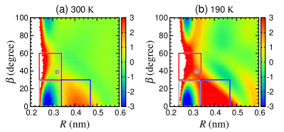
Figure 1: Contour plots of the potential of mean force, $W(R,\beta)$, at a temperature of 300 K (a) and 190 K (b). The value of the color bar is normalized by $k_{\mathrm{B}}T$. The saddle point is shown by the gray point. The rectangle indicated by the gray line represents the H-bond region. The areas surrounded by red and blue lines represent the H-bond breakage regions due to rotational and translational motions, respectively (denoted as regions R and T). The region with unsampled configurations is shown in white.

III Results and discussion

III.1 2D PMF and H-bond lifetimes

The 2D PMF contour plots are shown in Fig. 1 for $T=300$ K and $190$ K. The H-bond criterion is given by the geometrical condition between the two water molecules. Kumar, Schmidt, and Skinner (2007) Two molecules are considered H-bonded if the distance-angle relationship is $(0.24~{}\mathrm{nm},0^{\circ})\leq(R,\beta)\leq(0.34~{}\mathrm{nm},30^{\circ})$ (rectangular area indicated in Fig. 1). This criterion is mostly consistent with that reported previously. Kumar, Schmidt, and Skinner (2007) At shorter distance less than $R=0.24$ nm, the radial distribution functions $g_{\mathrm{OO}}(r)$ vanishes. The position $R=0.34$ nm corresponds to the first minima of $g_{\mathrm{OO}}(r)$. These threshold values remain unchanged at any temperature, as seen in Fig. 1. Figure 1 also shows that the temperature dependence of saddle point position is negligible. Instead, the roughness of the landscape becomes larger with decreasing the temperature and the free-energy difference $\Delta G^{\ddagger}$ between the global minimum and saddle point becomes correspondingly larger.

The transition from H-bonded to H-bond breakage states can be generally characterized by the saddle point on the free-energy surface. From our calculations, $(R^{\ddagger},\beta^{\ddagger})=(0.32~{}\mathrm{nm},39^{\circ})$ was obtained (indicated by the gray dot in Fig. 1). The H-bond is expected to be broken by increasing $\beta$, i.e., by exploiting molecular rotational motions. It is important to note that these 2D plots are not directly linked with $k_{\mathrm{TST}}$, which is the reactive flux at $t=0$ for a barrier-crossing dynamics with a dividing surface. The introduction of $k_{\mathrm{TST}}$ corresponds effectively to adopting a one-dimensional description of the reaction coordinate. On the other hand, a focus in the present work is to determine the TST-type expression, $\exp(-\Delta G^{\ddagger}/k_{\mathrm{B}}T)$, evaluated by referring to the saddle point on the 2D PMF profile. Although this expression does not definitely coincide with $k_{\mathrm{TST}}$, $\Delta G^{\ddagger}$ can be regarded as the Arrhenius activation energy $E_{\mathrm{A}}$ when it is independent of temperature over the dividing surface for the reactive flux and $\kappa$ is unity. Accordingly, the deviation from the Arrhenius behavior of $k=1/\tau_{\mathrm{HB}}$ has three sources: (1) the temperature dependence of $\Delta G^{\ddagger}$, which is concerned with the entropy of the activation; (2) the dimensionality of the reaction coordinate, which depends on the choice of reaction coordinate; and (3) the temperature dependence of $\kappa(<1)$, which reflects the detailed dynamics of barrier crossing. These issues are discussed in more detail.

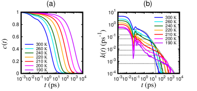
Figure 2: (a) H-bond correlation function $c(t)$. (b) Reactive flux $k(t)=-dc(t)/dt$. Dotted curves represent the exponential function $\exp(-t/\tau_{\mathrm{HB}})/\tau_{\mathrm{HB}}$ with H-bond lifetime $\tau_{\mathrm{HB}}$.

The H-bond correlation function $c(t)$ and reactive flux $k(t)$ are shown in Fig. 2. For comparison, the exponential decay curve $\exp(-t/\tau_{\mathrm{HB}})/\tau_{\mathrm{HB}}$ is plotted in Fig. 2(b). As mentioned in the end of Sec. II, the decay of $k(t)$ at longer times is characterized by the inverse of H-bond lifetime, $1/\tau_{\mathrm{HB}}$, at each temperature. These behaviors are consistent with previously reported results using SPC/E supercooled water. Starr, Nielsen, and Stanley (1999, 2000) The temperature dependence of $\tau_{\mathrm{HB}}$ is plotted in Fig. 3, where $\tau_{\mathrm{HB}}$ increases significantly with decreasing temperature. This drastic increase in $\tau_{\mathrm{HB}}$, particularly at supercooled states, has been recently reported using MD simulations. Kawasaki and Kim (2017) In particular, the temperature dependence shows Arrhenius behaviors, $\exp(E_{\mathrm{A}}/k_{\mathrm{B}}T)$, with different $E_{\mathrm{A}}$ values. As shown in Fig. 3, $E_{\mathrm{A}}$ increases with decreasing the temperature. The $E_{\mathrm{A}}$ were 17.9 and 39.6 kJ/mol at the high and low temperature regions, respectively. In contrast, the time scale $\tau_{\mathrm{s}}=1/k_{\mathrm{TST}}$ associated with the TST rate constant shows the Arrhenius temperature dependence, $\tau_{\mathrm{s}}\propto\exp(E_{\mathrm{s}}/k_{\mathrm{B}}T)$. The estimated Arrhenius activation energy was $E_{\mathrm{s}}=$ 9.7 kJ/mol, as shown in Fig. 3. Similar values of the activation energy have reported in other liquid water models, where the average of H-bond persistence lifetime was analyzed. Starr, Nielsen, and Stanley (1999, 2000); Martiniano and Galamba (2013); Galamba (2017) This persistence lifetime is relevant with the time scale of TST rate constant. Luzar (2000) These numerical results are also comparable with experimental values obtained from depolarized Rayleigh scattering. Conde and Teixeira (1984); Teixeira et al. (1985). Our observations indicate that the transmission coefficient $\kappa=k/k_{\mathrm{TST}}=\tau_{\mathrm{s}}/\tau_{\mathrm{HB}}$ decreases significantly when the temperature is lowered.

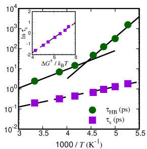
Figure 3: H-bond lifetime $\tau_{\mathrm{HB}}$ and inverse TST rate constant $\tau_{s}={k_{\mathrm{TST}}}^{-1}$ vs. inverse temperature $1000/T$. The Arrhenius behavior $\tau_{\mathrm{HB}}\propto\exp(E_{\mathrm{A}}/k_{\mathrm{B}}T)$ in the high and low temperature ranges are shown as two straight lines, with activation energies with $E_{\mathrm{A}}=$ 17.9 and 39.6 kJ/mol, respectively. The dashed line shows Arrhenius behavior for $\tau_{\mathrm{s}}\propto\exp(E_{\mathrm{s}}/k_{\mathrm{B}}T)$ with $E_{\mathrm{s}}=$ 9.7 kJ/mol. Inset: $\ln\tau_{\mathrm{s}}$ vs. the free-energy barrier of the saddle point $\Delta G^{\ddagger}/k_{\mathrm{B}}T$ on the 2D PMF profile. The dashed straight line is the fitting of $\tau_{\mathrm{s}}\propto\exp(C\Delta G^{\ddagger}/k_{\mathrm{B}}T)$ with a constant $C=0.7$.

Next, we investigated the relationship between $k_{\mathrm{TST}}$ and $\Delta G^{\ddagger}$ (note that $k_{\mathrm{TST}}$ is introduced as $k(0)$ in this work). Inset of Fig. 3 demonstrates the TST-type relationship, $\tau_{\mathrm{s}}\propto\exp(C\Delta G^{\ddagger}/k_{\mathrm{B}}T))$ with the slope about 0.7; the free-energy barrier corresponding to $k_{\mathrm{TST}}$ is underestimated considering the expected value of TST. We again note that the free-energy barrier of 2D PMF is a different quantity from that of the TST framework, which may have resulted in this underestimation. Another possible explanation is H-bond breakages due to non-trivial environmental effects around the tagged H-bonded molecules. Indeed, it has been demonstrated that molecular reorientations are occurred collectively. Laage and Hynes (2006) Such collective motions may have decreased the activation barrier lower than the TST prediction.

From the general expression, $k=\kappa k_{\mathrm{TST}}$, the non-Arrhenius behavior of $\tau_{\mathrm{HB}}(=1/k)$ and the increase in $E_{\mathrm{A}}$ with decreasing temperature are attributed to the temperature dependency of transmission coefficient $\kappa$, which considerably decreases with decreasing temperature (see Fig. 3). An analogous non-Arrhenius temperature dependence of $\tau_{\mathrm{HB}}$ has been demonstrated in TIP4P/2005 supercooled water. Kawasaki and Kim (2017) The physical implication of this is elucidated later.

III.2 Temporal development of H-bond distribution function

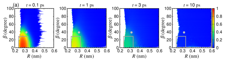
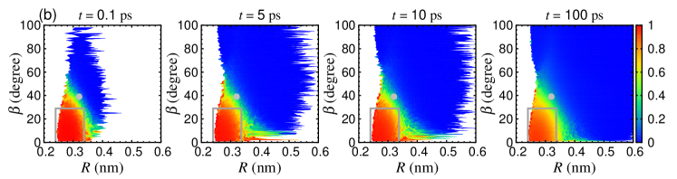
Figure 4: Conditional distance-angle distribution function $G(R,\beta;t)$ at temperatures of 300 K (a) and 190 K (b). The saddle point is shown by the gray point. The rectangle indicated by the gray line represents the H-bond region. The region with unsampled configurations is shown in white. (Multimedia view)

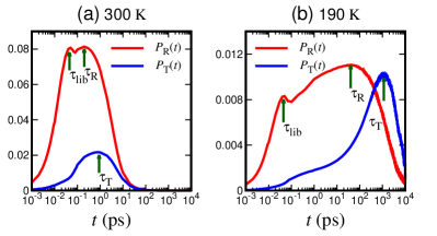
Figure 5: Time evolution of the normalized populations $P_{\mathrm{R}}(t)$ and $P_{\mathrm{T}}(t)$ for H-bond breakage regions at temperatures of 300 K (a) and 190 K (b). The H-bond breakage regions (regions R and T) are depicted in Fig. 1. Here, $\tau_{\mathrm{lib}}$, $\tau_{\mathrm{R}}$, and $\tau_{\mathrm{T}}$ are indicated by arrows.

To reveal the molecular mechanism of H-bond breakage in supercooled water, we examined the change of the geometric structure of two water molecules that are initially H-bonded. To this end, we propose the extension of $g(R,\beta)$ to the time dependent distribution function. Specifically, we introduce the conditional distribution function, $g(R,\beta;t|\mathrm{HB})$, which denotes the distance-angle distribution function of $(R,\beta)$ at time $t$ for a pair of water molecules located in the H-bonded region at an initial time $t=0$. Then, the time dependent ratio of the distance-angle distribution function is defined as follows,

$$G(R,\beta;t)=\frac{g(R,\beta;t|\mathrm{HB})}{g(R,\beta)}.$$ (1)

This function characterizes the evolution of the spatial correlations of the H-bond over time. Over longer times, the nonequilibrium distribution $g(R,\beta;t=0|\mathrm{HB})$ initially being inside the H-bond region finally recovers to that of the equilibrium distribution $g(R,\beta)$ because of the memory loss. More precisely, we observe $g(R,\beta;t|\mathrm{HB})\to(N_{\mathrm{HB}}/N)g(R,\beta)$ $(t\to\infty)$, where $N$ is the total number of molecules in the system and $N_{\mathrm{HB}}$ denotes the number of averaged accepted H-bonds calculated from integrating $g(R,\beta)$ over the H-bond region (denoted as region HB),

$$N_{\mathrm{HB}}=\int\int_{\mathrm{HB}}2\pi\rho R^{2}\sin\beta g(R,\beta)dRd\beta.$$ (2)

Note that $N_{\mathrm{HB}}$ ranged from from 1.7 ($T=300$ K) to 2.0 ($T=190$ K), which is not close to 4 since one of the water molecules has the O atom at the origin and acts only as the H-bond donor, while the H-bond angle $\beta$ is defined by considering the other water molecule as the H-bond acceptor. We also note that the present investigation is analogous to examining structural relaxation of the selected spectral using the hole-burning technique. Laenen, Rauscher, and Laubereau (1998)

Figure 4(Multimedia view) shows the time series of $G(R,\beta;t)$. At short time scales, the distribution is firstly elongated towards the angle direction (increasing $\beta$). This observation shows that the kinetic pathway of the H-bond breakage mainly passes through the saddle point on the 2D PMF profile. However, as the temperature is decreased, the penetration towards the distance direction (increasing $R$) becomes more apparent at longer time scales, showing transitions that do not pass through the saddle point. The random, but highly tetrahedral structures lead to frustrations in the H-bond networks in supercooled water. It is possible that these frustrations can be relaxed by collective molecular rearrangements, causing the translational jump motions. Ohmine and Tanaka (1993); Stanley et al. (1997); Giovambattista et al. (2004); Agmon (2012) Such collective rearrangements require larger activation energies. Furthermore, the 2D PMF using the distance-angle combinations of two-molecule geometry, $(R,\beta)$, does not show the saddle points consistent with the TST-type behavior.

The translational H-bond breakages are also regarded as the cage effects in glass-forming liquids, suggesting a transient environment around a tagged molecule surrounded by neighboring molecules. Doliwa and Heuer (1998); Weeks and Weitz (2002); Schweizer and Saltzman (2004); Shiba, Kawasaki, and Onuki (2012); Ciamarra, Pastore, and Coniglio (2016); Pastore et al. (2017) As demonstrated in various studies, there exists a plateau at an intermediate time regime in the translational mean square displacement of supercooled water, which is a manifestation of cage effects. Gallo et al. (1996); Sciortino et al. (1996); Giovambattista et al. (2004); Mazza et al. (2007); Kawasaki and Kim (2017) In fact, the decay of $c(t)$ at the time regime $\tau_{\mathrm{HB}}$ is dominated by the diffusion process. Starr, Nielsen, and Stanley (2000) Furthermore, the coupling between $\tau_{\mathrm{HB}}$ and the translational diffusion constant $D$ was suggested from the relationship $D\sim{\tau_{\mathrm{HB}}}^{-1}$ in TIP4P/2005 supercooled water. Kawasaki and Kim (2017)

III.3 Time scales of rotational and translational H-bond breakages

For the 2D PMF, it is impracticable to calculate the flux across a dividing surface as the kinetic pathway is not along a one-dimensional coordinate. As an alternative, the populations of non H-bond regions adjacent to the H-bonded region were quantified. For this purpose, we define the rectangular H-bond breakage regions, as described in Fig. 1. The H-bond breakage region due to rotational motions (increasing the angle $\beta$) is defined as $(0.24~{}\mathrm{nm},30^{\circ})<(R,\beta)<(0.34~{}\mathrm{nm},60^{\circ})$, where this region is denoted by R. The H-bond breakage region due to translational motions (increasing the distance $R$) is also defined as $(0.34~{}\mathrm{nm},0^{\circ})<(R,\beta)<(0.47~{}\mathrm{nm},30^{\circ})$, denoted as region T. Note that the area of the H-bond breakage region obtained from the integral $2\pi R^{2}\sin\beta$ is same for regions R and T. The population of each region was calculated using:

$$N_{i}(t)=\int\int_{i}2\pi\rho R^{2}\sin\beta g(R,\beta;t|\mathrm{HB})dRd\beta,$$ (3)

where $i$ represents the symbol of the region ($i\in${HB, R, T}). Normalization by the number of averaged accepted H-bonds, $N_{\mathrm{HB}}$, is defined as $P_{i}(t)\equiv N_{i}(t)/N_{\mathrm{HB}}$. Note that $P_{\mathrm{HB}}(t)=N_{\mathrm{HB}}(t)/H_{\mathrm{HB}}$ is equivalent to the H-bond correlation function $c(t)$ from the definition. We also note that the sum, $P_{\mathrm{HB}}(t)+P_{\mathrm{R}}(t)+P_{\mathrm{T}}(t)$, is not a conserved quantity; it begins as unity at $t=0$ ($P_{\mathrm{HB}}(0)=1$ and $P_{\mathrm{R}}(0)=P_{\mathrm{T}}(0)=0$) and decays to zero as the populations inside the regions R and T at time $t$ will spontaneously migrate to other non H-bond states afterwards.

Figure 5 shows the time evolution of the normalized population, $P_{i}(t)(=N_{i}(t)/N_{\mathrm{HB}})$. Both $P_{\mathrm{R}}(t)$ and $P_{\mathrm{T}}(t)$ started from zero and increases with time $t$. This regime indicates that the inflow due to the H-bond breakage exceeds the outflow towards other non H-bond states. For $P_{\mathrm{R}}(t)$, we observed additional peaks at around $\tau_{\mathrm{lib}}\lesssim 0.1$ ps, which are independent of the temperature, attributed to libration motion. They eventually decay to zero after a peak time, where the outflow exceeds the inflow for longer time scales. That is, the maximum peaks are determined by the balance. Thus, the peak times of $P_{\mathrm{R}}(t)$ and $P_{\mathrm{T}}(t)$ (denoted as $\tau_{\mathrm{R}}$ and $\tau_{\mathrm{T}}$, respectively) can be regarded as the characteristic time scales of irreversible H-bond breakages due to rotational and translational motions, respectively. It should be noted that the pathways going from region R(T) to T(R) were not detected. In fact, the H-bond breakages for time regimes at either $\tau_{\mathrm{R}}$ or $\tau_{\mathrm{T}}$ are irreversible for a particular pair of water molecules and two water molecules hardly reform the same H-bond pair. We observed that there existed a population of the translational H-bond breakage, even at higher temperatures. The peak value of $P_{\mathrm{T}}(t)$ becomes comparable to that of $P_{\mathrm{R}}(t)$ with decreasing the temperature. This indicates the increasing number of pathways not going through the saddle point on the 2D PMF profile, particularly for supercooled water.

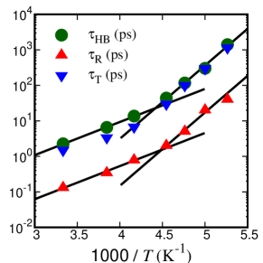
Figure 6: Temperature dependence of the maximum times in $P_{\mathrm{R}}(t)$ and $P_{\mathrm{T}}(t)$, as denoted by $\tau_{\mathrm{R}}$ and $\tau_{\mathrm{T}}$, respectively. Comparisons with $\tau_{\mathrm{HB}}$ are also shown. The straight lines represent Arrhenius behavior $\exp(E_{\mathrm{A}}/k_{\mathrm{B}}T)$ in the high and low temperature ranges with activation energies with $E_{\mathrm{A}}=$ 17.9 and 39.6 kJ/mol, respectively.

The temperature dependence of $\tau_{\mathrm{R}}$ and $\tau_{\mathrm{T}}$ is plotted in Fig. 6. It can be seen that $\tau_{\mathrm{T}}$ is comparable with $\tau_{\mathrm{HB}}$ at all studied temperatures. In contrast, the time scale of $\tau_{\mathrm{R}}$ is about one order of magnitude smaller than $\tau_{\mathrm{T}}$ although the temperature dependence of $\tau_{\mathrm{R}}$ shows similar Arrhenius behaviors. These observations indicate that the H-bond lifetime $\tau_{\mathrm{HB}}$ is dominated by the H-bond breakages caused by translational motions. Finally, this observation $\tau_{\mathrm{T}}\simeq\tau_{\mathrm{HB}}$ results in the following implication for the temperature dependence of $\kappa$;

$$\frac{1}{\kappa}=\frac{\tau_{\mathrm{HB}}}{\tau_{\mathrm{s}}}\propto\tau_{\mathrm{T}}\exp\left(-\frac{C\Delta G^{\ddagger}}{k_{\mathrm{B}}T}\right).$$ (4)

This relationship is direct evidence that the temperature dependence of $\kappa$ is caused by that of the time scale of H-bond breakage due to translational motions.

IV Conclusions

We analyzed the H-bond breakage dynamics in the TIP4P supercooled water considering a geometric definition of the H-bond. We first investigated the temperature dependence of the 2D PMF obtained from the distance-angle distribution function. It was found that the position of the saddle point distinguishing H-bond and non H-bond regions remains unchanged at all the temperatures studied, while the free-energy barrier of the saddle point, $\Delta G^{\ddagger}$, gradually increased with decreasing temperature. We showed that the Arrhenius activation energy of $\tau_{\mathrm{HB}}$ increases with decreasing temperature. In contrast, the TST rate constant $k_{\mathrm{TST}}$ of the H-bond breakage approximately followed the Arrhenius temperature dependence. In addition, the TST-type expression, $\exp(-C\Delta G^{\ddagger}/k_{\mathrm{B}}T)$, was obtained, where the correction factor $C$ was temperature independent. This suggests a significant decrease in the transmission coefficient $\kappa$ with decreasing temperature.

To elucidate the molecular mechanism of H-bond breakage, the kinetic pathways of H-bond breakage were studied. In particular, the time dependence of the conditional distance-angle distribution function revealed the pathways that did not go through the saddle point when the system was deeply supercooled, which was attributed to H-bond breakages due to translational motions. This translational H-bond breakage is thought to be associated with the cage-jump motion, which is commonly observed in various glass-forming liquids. In addition, it is proposed that the avalanches of cage-jump motions trigger collective molecular motions, referred to as dynamic heterogeneities. Our observations indicated that such collective motions involving many molecules were not described well by the present 2D PMF using geometric variables defined by the water dimer.

Furthermore, we quantified the time dependent populations of the rotational and translational H-bond breakages. With decreasing temperature, the population of the translational H-bond breakage became comparable to that of the rotational H-bond breakage passing through the saddle point. In particular, the time scale of the translational H-bond breakage $\tau_{\mathrm{T}}$ became much longer than that of the rotational H-bond breakage $\tau_{\mathrm{R}}$. The temperature dependence of the H-bond lifetime $\tau_{\mathrm{HB}}$ was comparable to that of $\tau_{\mathrm{T}}$. This suggests that the H-bond lifetime $\tau_{\mathrm{HB}}$ is dominated by the translational motions.

Finally, we note that it is important to investigate whether the 2D PMF associated with H-bonds and their breakages is suitable for supercooled water. In fact, Sciortino et al. demonstrated that the bifurcated H-bond configuration promotes H-bond breakages with high mobility Sciortino, Geiger, and Stanley (1991, 1992), which is apparently “hidden” in the 2D PMF drawn for a pair of water molecules; a bifurcated bond can be explicitly described only beyond the pair level. Our observations suggested that there exists another possible saddle point on the 2D PMF profile that reflects the translational H-bond breakage relevant with the bifurcated bonds. Hence, the profile of the PMF might be appropriately transformed, even with the same reaction coordinates, by using information regarding the kinetic pathways from the H-bond to the non H-bond regions. We are currently undertaking further investigations to clarify this issue.