fficient Fuzzing by Principled Search

Abstract

Fuzzing is a popular technique for finding software bugs. However, the performance of the state-of-the-art fuzzers leaves a lot to be desired. Fuzzers based on symbolic execution produce quality inputs but run slow, while fuzzers based on random mutation run fast but have difficulty producing quality inputs. We propose new mutation-based fuzzer that outperforms the state-of-the-art fuzzers by a wide margin. The main goal of to increase branch coverage by solving path constraints without symbolic execution. To solve path constraints efficiently, we introduce several key techniques: scalable byte-level taint tracking, context-sensitive branch count, search based on gradient descent, and input length exploration. On the LAVA-M data set, und almost all the injected bugs, found more bugs than any other fuzzer that we compared with, and found eight times as many bugs as the second-best fuzzer in the program who. so found 103 bugs that the LAVA authors injected but could not trigger. We also tested eight popular, mature open source programs. und 6, 52, 29, 40 and 48 new bugs in file, jhead, nm, objdump and size, respectively. We measured the coverage of d evaluated how its key techniques contribute to its impressive performance.

1 Introduction

Fuzzing is a popular technique for finding software bugs. Coverage-based fuzzers face the key challenge of how to create inputs to explore program states. Some fuzzers use symbolic execution to solve path constraints [5, 8], but symbolic execution is slow and cannot solve many types of constraints efficiently [6]. To avoid these problems, AFL uses no symbolic execution or any heavy weight program analysis [1]. It instruments the program to observe which inputs explore new program branches, and keeps these inputs as seeds for further mutation. AFL incurs low overhead on program execution, but most of the inputs that it creates are ineffective (i.e., they fail to explore new program states) because it blindly mutates the input without taking advantage of the data flow in the program. Several fuzzers added heuristics to AFL to solve simple predicates, such as “magic bytes” [25, 19], but they cannot solve other path constraints.

We designed and implemented a fuzzer, called , that explores the states of a program by solving path constraints without using symbolic execution. acks the unexplored branches and tries to solve the path constraints on these branches. We introduced the following techniques to solve path constraints efficiently.

TABLE I: Bugs found on the LAVA-M data set by different fuzzers. Note that und more bugs than listed by LAVA authors.

Program	Listed	Bugs found by each fuzzer
	bugs		AFL	FUZZER	SES	VUzzer	Steelix
uniq	$28$	$29$	$9$	$7$	$0$	$27$	$7$
base64	$44$	$48$	$0$	$7$	$9$	$17$	$43$
md5sum	$57$	$57$	$0$	$2$	$0$	Fail	$28$
who	$2136$	$1541$	$1$	$0$	$18$	$50$	$194$

• Context-sensitive branch coverage. AFL uses context-insensitive branch coverage to approximate program states. Our experience shows that adding context to branch coverage allows explore program states more pervasively (Section 3.2).

• Scalable byte-level taint tracking. Most path constraints depend on only a few bytes in the input. By tracking which input bytes flow into each path constraint, tates only these bytes instead of the entire input, therefore reducing the space of exploration substantially (Section 3.3).

• Search based on gradient descent. When mutating the input to satisfy a path constraint, oids symbolic execution, which is expensive and cannot solve many types of constraints. Instead, es the gradient descent algorithm popular in machine learning to solve path constraints (Section 3.4).

• Type and shape inference. Many bytes in the input are used collectively as a single value in the program, e.g., a group of four bytes in the input used as a 32-bit signed integer in the program. To allow gradient descent to search efficiently, cates the above group and infers its type (Section 3.5).

• Input length exploration. A programs may explore certain states only when the length of the input exceeds some threshold, but neither symbolic execution nor gradient descent can tell the fuzzer when to increase the length of the input. tects when the length of the input may affect a path constraint and then increases the input length adequately (Section 3.6).

tperformed state-of-the-art fuzzers substantially. Section 1 compares the bugs found by th other fuzzers on the LAVA-M data set [9]. und more bugs in each program in the data set. Particularly, in who und 1541 bugs, which is eight times as many bugs as found by the second-best fuzzer, Steelix. Moreover, und 103 bugs that the LAVA authors injected but could not trigger. We also tested eight popular, mature open source programs. und 6, 52, 29, 40 and 48 new bugs in file, jhead, nm, objdump and size, respectively (Table V). We measured the coverage of d evaluated how its key techniques contribute to its impressive performance.

2 Background: American Fuzzy Lop (AFL)

Fuzzing is an automated testing technique to find bugs. American Fuzzy Lop (AFL) [1] is a state-of-the-art mutation-based graybox fuzzer. AFL employs light-weight compile-time instrumentation and genetic algorithms to automatically discover test cases that likely trigger new internal states in the targeted program. As a coverage-based fuzzer, AFL generates inputs to traverse different paths in the program to trigger bugs.

2.1 Branch coverage

AFL measures a path by a set of branches. During each run, AFL counts how many times each branch executes. It represents a branch as a tuple ($l_{\mathrm{prev}},l_{\mathrm{cur}}$), where $l_{\mathrm{prev}}$ and $l_{\mathrm{cur}}$ are the IDs of the basic blocks before and after the conditional statement, respectively. AFL gets the branch coverage information by using lightweight instrumentation. The instrumentation is injected at each branch point at compile time. For each run, AFL allocates a path trace table to count how many times each branch of every conditional statement executes. The index to the table is the hash of a branch, $h(l_{\mathrm{prev}},l_{\mathrm{cur}})$, where $h$ is a hash function.

AFL also keeps a global branch coverage table across different runs. Each entry contains an 8-bit vector that records how many times the branch executes in different runs. Each bit in this vector $b$ represents a range: $b_{0},\ldots,b_{7}$ represent the ranges $[1]$, $[2]$, $[3]$, $[4,7]$, $[8,15]$, $[16,31]$, $[32,127]$, $[128,\infty)$, respectively. For example, if $b_{3}$ is set, then it indicates that there exists a run where this branch executed between 4 and 7 times, inclusively.

AFL compares the path trace table and branch coverage table to determine, heuristically, whether a new input triggers a new internal state of the program. An input triggers a new internal state if either of the following happens:

• The program executes a new branch, i.e., the path trace table has an entry for this branch but the branch coverage table has no entry for this branch.

• There exists a branch where the number of times, $n$, this branch executed in the current run is different from any previous runs. AFL determines this approximately by examining whether the bit representing the range of $n$ was set in the corresponding bit vector in the branch coverage table.

2.2 Mutation strategies

AFL applies the following mutations on the input randomly [3].

• Bit or byte flips.

• Attempts to set “interesting” bytes, words, or dwords.

• Addition or subtraction of small integers to bytes, words, or dwords.

• Completely random single-byte sets.

• Block deletion, block duplication via overwrite or insertion, or block memset.

• Splice two distinct input files at a random location.

3 Design

3.1 Overview

1:function Fuzz($program,seeds$)

2:     Instrument $program$ in two versions: $program_{\mathrm{nt}}$ (no taint tracking) and $program_{\mathrm{t}}$ (with taint tracking).

3:     $branches\leftarrow$ empty hash table $\triangleright$ Key: an unexplored branch $b$. Value: the input that explored $b$’s sibling branch.

4:     for all $input\in seeds$ do

5:         $path\leftarrow$ Run $program_{\mathrm{t}}(input)$

6:         for all unexplored branch $b$ on $path$ do

7:              $branches[b]\leftarrow input$

8:         end for

9:     end for

10:     while $branches\not=\emptyset$ do

11:         Select $b$ from $branches$

12:         while $b$ is still unexplored do

13:              Mutate $branches[b]$ to get a new input $input^{\prime}$ (Algorithm 5)

14:              Run $program_{\mathrm{nt}}(input^{\prime})$

15:              if $input^{\prime}$ explored new branches then

16:                  $path^{\prime}\leftarrow$ Run $program_{\mathrm{t}}(input^{\prime})$

17:                  for all unexplored branch $b^{\prime}$ on $path^{\prime}$ do

18:                       $branches[b^{\prime}]\leftarrow input^{\prime}$

19:                  end for

20:              end if

21:              if $b$ was explored then

22:                  $branches\leftarrow branches-\{b\}$

23:              end if

24:         end while

25:     end while

26:end function

Algorithm 1 fuzzing loop. Each while loop has a budget (maximum allowed number of iterations)

AFL and other similar fuzzers use branch coverage as the metric. However, they fail to consider the call context when calculating branch coverage. Our experience shows that without context, branch coverage would fail to explore program states adequately. Therefore, we propose context-sensitive branch coverage as the metric of coverage (Section 3.2).

Algorithm 1 shows two stages: instrumentation and the fuzzing loop. During each iteration of the fuzzing loop, lects an unexplored branch and searches for an input that explores this branch. We introduce the following key techniques to find the input efficiently.

• For most conditional statements, its predicate is influenced by only a few bytes in the input, so it would be unproductive to mutate the entire input. Therefore, when exploring a branch, termines which input bytes flow into the corresponding predicate and focuses on mutating these bytes only (Section 3.3).

• After determining which input bytes to mutate, eds to decide how to mutate them. Using random or heuristics-based mutations is unlikely to find satisfactory values efficiently. Instead, we view the path constraint on a branch as a constraint on a blackbox function over the input, and we adapt the gradient descent algorithm for solving the constraint (Section 3.4).

• During gradient descent, we evaluate the blackbox function over its arguments, where some arguments consist of multiple bytes. For example, when four consecutive bytes in the input that are always used together as an integer flow into a conditional statement, we ought to consider these four bytes as a single argument to the function instead of as four independent arguments. To achieve this goal, we need to infer which bytes in the input are used collectively as a single value and what the type of the value is (Section 3.5).

• It would be inadequate to only mutate bytes in the input. Some bugs are triggered only after the input is longer than a threshold, but this creates a dilemma on deciding the length of the input. If the input is too short, it may not trigger certain bugs. But if the input is too long, the program may run too slow. Most fuzzers change the length of inputs using ad hoc approaches. By contrast, struments the program with code that detects when a longer input may explore new branches and that determines the minimum required length (Section 3.6).

Figure 1 shows a diagram of the steps in fuzzing a conditional statement. The program in Figure 2 demonstrates these steps in action.

• Byte-level taint tracking: When fuzzing the conditional statement on Line 2, using byte-level taint tracking, termines that bytes 1024–1031 flow into this expression, so it mutates these bytes only.

• Search algorithm based on gradient descent: eds to find inputs that run both branches of the conditional statement on Line 2, respectively. eats the expression in the conditional statement as a function $f(\mathbf{x})$ over the input $\mathbf{x}$, and uses gradient descent to find two inputs $\mathbf{x}$ and $\mathbf{x}^{\prime}$ such that $f(\mathbf{x})>0$ and $f(\mathbf{x}^{\prime})\leq 0$.

• Shape and type inference: $f(\mathbf{x})$ is a function over the vector $\mathbf{x}$. During gradient descent, mputes the partial derivative of $f$ over each component of $\mathbf{x}$ separately, so it must determine each component and its type. On Line 2, termines that $\mathbf{x}$ consists of two components each consisting of four bytes in the input and having the type 32-bit signed integer.

• Input length exploration: main will not call foo unless the input has at least 1032 bytes. Instead of blindly trying longer inputs, we instrument common functions that read from input and determine if longer input would explore new states. For example, if the initial input is shorter than 1024 bytes, then the conditional statement on Line 12 will execute the true branch. Since the return value of fread is compared with 1024, ows that only inputs at least 1024 bytes long will explore the false branch. Similarly, the instrumentation on Lines 16 and 19 instructs extend the input to at least 1032 bytes to execute the function foo.

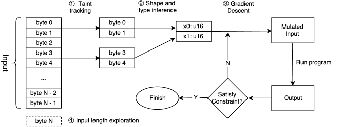
Figure 1: Steps in fuzzing a conditional statment.

⬇

1void foo(int i, int j) {

2 if (i * i - j * 2 > 0) {

3 // some code

4 } else {

5 // some code

6 }

7}

8

9int main() {

10 char buf[1024];

11 int i = 0, j = 0;

12 if(fread(buf, sizeof(char), 1024, fp)

13 < 1024) {

14 return(1);

15 }

16 if(fread(&i, sizeof(int), 1, fp) < 1){

17 return(1);

18 }

19 if(fread(&j, sizeof(int), 1, fp) < 1){

20 return(1);

21 }

22 foo(i, j);

23}

Figure 2: Example program showing core techniques

3.2 Context-sensitive branch count

Section 2 describes AFL’s branch coverage table. Its design has several advantages. First, it is space efficient. The number of branches is linear in the size of the program. Second, using ranges to count branch execution provides good heuristics on whether a different execution count indicates new internal state of the program. When the execution count is small (e.g., less than four), any change in the count is significant. However, when the execution count is large (e.g., greater than 32), a change has to be large enough to be considered significant.

But this design has a limitation. Because AFL’s branches are context-insensitive, they fail to distinguish the executions of the same branch in different contexts, which may overlook new internal states of the program. Figure 3 illustrates this problem. Consider the coverage of the branch on Line 3. During the first run, the program takes the input “10”. When it calls f() on Line 19, it executes the true branch on Line 4. Later, when it calls f() on Line 21, it executes the false branch on Line 10. Since AFL’s definition of branch is context-insensitive, it thinks that both branches have executed. Later, when the program takes a new input “01”, AFL thinks that this input triggers no new internal state, since both the branches on Line 4 and 10 executed in the previous run. But in fact this new input triggers a new internal state, as it will cause crash on Line 6 when input[2]==1.

⬇

1void f(bool x) {

2 static bool trigger = false;

3 if (x) {

4 if (trigger) {

5 if (input[2]) {

6 // crash;

7 }

8 }

9 } else {

10 if (!trigger) {

11 trigger = true;

12 }

13 }

14}

15

16bool[] input;

17

18int main() {

19 f(input[0]);

20 ...

21 f(input[1]);

22}

Figure 3: Example where context-insensitive branch count fails to detect new behavior

We incorporate context into the definition of branches. We define a branch as a tuple $(l_{\mathrm{prev}},l_{\mathrm{cur}},context)$, where $l_{\mathrm{prev}}$ and $l_{\mathrm{cur}}$ are the IDs of the basic blocks before and after the conditional statement, respectively, $context$ is $h(stack)$ where $h$ is a hash function, and $stack$ contains the state of the call stack. For example, let the program in Figure 3 first run on the input 10. After it enters f() from Line 19, it will execute the branch $(l_{\ref{lst:branch}},l_{\ref{lst:true}},[l_{\ref{lst:caller1}}])$. Then, after it enters f() from Line 21, it will execute the branch $(l_{\ref{lst:branch}},l_{\ref{lst:false}},[l_{\ref{lst:caller2}}])$. By contrast, when the program executes on the input “01”, it will execute the branches $(l_{\ref{lst:branch}},l_{\ref{lst:false}},[l_{\ref{lst:caller1}}])$ followed by $(l_{\ref{lst:branch}},l_{\ref{lst:true}},[l_{\ref{lst:caller2}}])$. By incorporating calling context into the definition of branch, n detect that the second run triggers a new internal state, which will lead to the crash site on Line 6 when mutating input[2].

Adding context to branches increases the number of unique branches, which could be dramatic when deep recursion occurs. Our current implementation mitigates this problem by selecting a particular function $h$ for computing the hash of the call stack where $h$ computes the xor of the IDs of all the call sites on the stack. When struments the program, it assigns a random ID to each call site. Therefore, when a function f recursively calls itself, no matter how many times shes the ID of the same call site to the call stack, $h(stack)$ outputs at most two unique values, which at most doubles the number of unique branches in the function f. Our evaluation on real world programs shows that after incorporating context, the number of unique branches increases by as many as 7.21 times (Table VII) in exchange for the benefit of improved code coverage (Figure 7).

3.3 Byte-level taint tracking

The objective of to create inputs to execute unexplored branches. When it tries to execute an unexplored branch, it must know which byte offsets in the input affect the predicate of the branch. Therefore, quires byte-level taint tracking. However, taint tracking is expensive, especially when tracking each byte individually, so AFL avoids it. Our key insight is that taint tracking is unnecessary on most runs of the program. Once we run taint tracking on an input (Step 1 in Figure 1), we can record which byte offsets flow into each conditional statement. Then, when we mutate these bytes, we can run the program without taint tracking. This amortizes the cost of taint tracking on one input over its many mutations, which allows have a similar throughput of input execution as AFL (Section 5.6).

sociates each variable $x$ in the program with a taint label $t_{x}$, which represents the byte offsets in the input that may flow into $x$. The data structure of taint labels has a big impact on its memory footprint. A naive implementation would be to represent each taint label as a bit vector, where each bit $i$ represents the $i$th byte in the input. However, since the size of this bit vector grows linearly in the size of the input, this data structure would be prohibitive for large input, but large input is necessary for finding bugs in certain programs.

To reduce the size of the taint labels, we could store the bit vectors in a table, and use the indices to the table as taint labels. As long as the logarithm of the number of entries in the table is much less than the length of the longest bit vectors, which is often the case, we can greatly reduce the size of the taint labels.

However, this data structure raises a new challenge. The taint labels must support the following operations:

• Insert($b$): inserts a bit vector $b$ and returns its label.

• Find($t$): returns the bit vector of the taint label $t$.

• Union($t_{x},t_{y}$): returns the taint label representing the union of the bit vectors of the taint labels $t_{x}$ and $t_{y}$.

Find is cheap, but union is expensive. union takes the following steps. First, it finds the bit vectors of the two labels and computes their union $u$. This step is cheap. Next, it searches the table to determine if $u$ already exists. If not, it adds $u$. But how to search efficiently? A linear search would be expensive. Alternatively, we could build a hash set of the bit vectors, but if there are a lot of them and each bit vector is long, it would take much time to compute the hash code and much space to store the hash set. Since union is a common operation when we track tainted data in arithmetic expressions, it must be efficient. Note that we cannot use the union-find data structure because the vectors are not disjoint, i.e., two different bit vectors may have 1 at the same position.

We propose a new data structure for storing the bit vectors that allows efficient insert, find and union. For each bit vector, the data structure assigns it a unique label using an unsigned integer. When the program inserts a new bit vector, the data structure assigns it the next available unsigned integer.

The data structure contains two components.

• A binary tree maps bit vectors to their labels. Each bit vector $b$ is represented by a unique tree node $v_{b}$ at level $|b|$, where $|b|$ is the length of $b$. $v_{b}$ stores the label of $b$. To reach $v_{b}$ from the root, examine $b_{0},b_{1},\ldots$ sequentially. If $b_{i}$ is 0, go to the left child; otherwise, go to the right child. Each node contains a back pointer to its parent to allow us to retrieve the bit vector starting from $v_{b}$.

• A look up table maps labels to their bit vectors. A label is an index to this table, and the corresponding entry points to the tree node representing the bit vector of this label.

In this data structure, all leaves in the tree represent bit vectors, and no internal node represents bit vectors. However, many nodes in the tree may be unnecessary. For example, if a vector $x00*$ is in the tree but no vector $x0[01]*1[01]*$ is in the tree, where $x$ is any sequence of bits, then it would be unnecessary to store any node after the node representing $x$, because $x$ has only one decedent that is a leaf, and this leaf represents $x00*$. Here we use the common notation for regular expressions where $x*$ means that $x$ is repeated zero or more times, and $[xy]$ means either $x$ or $y$. This observation allows us to trim a vector when inserting it into a tree as follows:

1. Remove all the trailing 0s of the vector.

2. Follow the bits in the vector, from the first to the last bit, to traverse the tree.

   • If a bit is 0, follow the left child

   • Otherwise, follow the right child.

   If a child is missing, create it.

3. Store the label of the vector in the last node we visited.

Algorithm 2 describes this insert operations in detail. Algorithm 3 and Algorithm 4 describe the find and union operations, respectively. Note that when we create a node, initially it contains no label. Later, if this node is the last node visited when we insert a bit vector, we store the label of the bit vector in this node. With this optimization, this tree has the following properties:

• Each leaf node contains a label.

• An internal node may contain a label. We may store a label in an internal node that has no label yet, but we never replace the label in any internal node.

1:function insert($root,vector,nodes$) $\triangleright$ $root$: root of the tree. $vector$: the vector to be inserted. $nodes$: an array indexed by labels containing pointers to tree nodes. $return$: the label representing $vector$.

2:     Trims all the trailing 0s in $vector$

3:     if $vector$ is empty then

4:         if $root$ contains no label then

5:              $root.label\leftarrow nodes.length()$ $\triangleright$ Assigns the next available integer as the label for this vector.

6:              $nodes.push(root)$

7:         end if

8:         return $root.label$

9:     end if

10:     if $vector[0]==0$ then

11:         $node\leftarrow root.left$

12:     else

13:         $node\leftarrow root.right$

14:     end if

15:     if $node$ does not exist then

16:         Creates $node$

17:         if $|vector|==1$ then

18:              $node.label=nodes.length()$ $\triangleright$ Assigns the next available integer as the label for this vector.

19:              $nodes.push(node)$

20:         end if

21:     end if

22:     if $|vector|==1$ then

23:         return $node.label$

24:     else

25:         return insert($node,vector[1..],nodes$) $\triangleright$ $vector[1..]$ is $vector$ after first element removed.

26:     end if

27:end function

Algorithm 2 Insert a bit vector into the tree

1:function find($label,nodes$) $\triangleright$ $label$: an integer representing a tree node, which represents a bit vector. $nodes$: an array indexed by labels and containing pointers to tree nodes. $return$: the bit vector represented by $label$.

2:     $vector\leftarrow$ empty vector

3:     $node\leftarrow nodes[label]$

4:     $parent\leftarrow node.parent$

5:     while $parent$ exists do

6:         if $node$ is the left child of $parent$ then

7:              $vector.insert\_at\_beginning(0)$

8:         else

9:              $vector.insert\_at\_beginning(1)$

10:         end if

11:         $node\leftarrow parent$

12:         $parent\leftarrow node.parent$

13:     end while

14:     return vector

15:end function

Algorithm 3 Find a bit vector by its label

1:function union($label_{1},label_{2},nodes,root$) $\triangleright$ $label_{1},label_{2}$: labels of two bit vectors. $nodes$: a table containing pointers to tree nodes. $root$: root of the tree. Return: the label representing the union of the bit vectors.

2:     $v_{1}\leftarrow\mbox{{find}}(label_{1},nodes)$

3:     $v_{2}\leftarrow\mbox{{find}}(label_{2},nodes)$

4:     $v\leftarrow v_{1}\cup v_{2}$

5:     return insert($root,v,nodes$)

6:end function

Algorithm 4 Union two bit vectors

This data structure greatly reduces the memory footprint for storing the bit vectors. Let the length of each bit vector be $n$, and let there be $l$ bit vectors. If we naively store all the bit vectors in a look up table, it would take $O(nl)$ space. However, in our data structure, the number of nodes in the tree is $O(l)$. Each node may store at most one index to the look up table. Since the look up table has $l$ entries and each entry is a pointer and so has a fixed size, the size of the look up table is $O(l)$, and each index to the look up table has $O(\log l)$ bits. Therefore, the total space requirement is $O(l\cdot\log l)$.

3.4 Search algorithm based on gradient descent

Byte-level taint tracking discovers which byte offsets in the input flow into a conditional statement. But how to mutate the input to run the unexplored branch of the statement? Most fuzzers mutate the input randomly or using crude heuristics, but those strategies are unlikely to find an appropriate input value quickly. By contrast, we view this as a search problem and take advantage of search algorithms in machine learning. We used gradient descent in our implementation, but other search algorithms might also work.

In this approach, we view the predicate for executing a branch as a constraint on a blackbox function $f(\mathbf{x})$, where $\mathbf{x}$ is a vector of the values in the input that flow into the predicate, and $f()$ captures the computation on the path from the start of the program to this predicate. There are three types of constraints on $f(\mathbf{x})$:

1. $f(\mathbf{x})<0$.

2. $f(\mathbf{x})<=0$.

3. $f(\mathbf{x})==0$.

Table II shows that we can transform all forms of comparison into the above three types of constraints. If the predicate of a conditional statement contains logical operators && or ||, lits the statement into multiple conditional statements. For example, it splits if (a && b) { s } else { t } into if (a) { if (b) {s} else {t} } else {t} .

TABLE II: Transforming comparisons into constraints. $a$ and $b$ represent arbitrary expressions.

Comparison	f	Constraint
$a<b$	$f=a-b$	$f<0$
$a<=b$	$f=a-b$	$f<=0$
$a>b$	$f=b-a$	$f<0$
$a>=b$	$f=b-a$	$f<=0$
$a==b$	$f=abs(a-b)$	$f==0$
$a!=b$	$f=-abs(a-b)$	$f<0$

Algorithm 5 shows the search algorithm. Starting from an initial $\mathbf{x_{0}}$, find $\mathbf{x}$ such that $f(\mathbf{x})$ satisfies the constraint. Note that to satisfy each type of constraint, we need to minimize $f(\mathbf{x})$, and we use gradient descent for this purpose.

Gradient descent finds a minimum of a function $f(\mathbf{x})$. The method is iterative. Each iteration starts from an $\mathbf{x}$, computes $\nabla_{\mathbf{x}}f(\mathbf{x})$ (the gradient of $f(\mathbf{x})$ at $\mathbf{x}$), and updates $\mathbf{x}$ as $\mathbf{x}-\epsilon\nabla_{\mathbf{x}}f(\mathbf{x})$ where $\epsilon$ is the learning rate.

When training neural networks, researchers use gradient descent to find a set of weights that minimize the training error. However, gradient descent has the problem that it sometimes may be stuck in a local minimum that is not a global minimum. Fortunately, this is often not a problem in fuzzing, because we only need to find an input $\mathbf{x}$ that is good enough instead of a globally optimal $\mathbf{x}$. For example, if the constraint is $f(\mathbf{x})<0$, then we just need to find an $\mathbf{x}$ where $f(\mathbf{x})<0$ instead of where $f(\mathbf{x})$ is a global minimum.

However, we face unique challenges when applying gradient descent to fuzzing. Gradient descent requires computing the gradient $\nabla_{\mathbf{x}}f(\mathbf{x})$. In neural networks, we can write $\nabla_{\mathbf{x}}f(\mathbf{x})$ in an analytic form. However, in fuzzing, we have no analytic form of $f(\mathbf{x})$. Second, in neural networks, $f(\mathbf{x})$ is a continuous function because $\mathbf{x}$ contains the weights of the network, but in fuzzing $f(\mathbf{x})$ is usually a discrete function. This is because most variables in a typical program are discrete, so most elements in $\mathbf{x}$ are discrete.

We solve these problems using numerical approximation. The gradient of $f(\mathbf{x})$ is the unique vector field whose dot product with any unit vector $\mathbf{v}$ at each point $\mathbf{x}$ is the directional derivative of $f$ along $\mathbf{v}$. We approximate each directional derivative by $\frac{\partial f(\mathbf{x})}{\partial\mathbf{x}_{i}}=\frac{f(\mathbf{x}+\delta\mathbf{v}_{i})-f(\mathbf{x})}{\delta}$ where $\delta$ is a small positive value (e.g., 1) and $\mathbf{v}_{i}$ is the unit vector in the $i$th dimension. To compute each directional derivative, we need to run the program twice, once with the original input $\mathbf{x}$ and once with the perturbed input $\mathbf{x}+\delta\mathbf{v}_{i}$. It is possible that in the second run, the program fails to reach the program point where $f(\mathbf{x}+\delta\mathbf{v}_{i})$ is calculated because the program took a different branch at an earlier conditional statement. When this happens, we set $\delta$ to a small negative value (e.g., -1) and try to compute $f(\mathbf{x}+\delta\mathbf{v}_{i})$ again. If this succeeds, we compute the directional derivative based on it. Otherwise, we set the derivative to zero, instructing gradient descent not to move $\mathbf{x}$ in this direction. The time for computing the gradient is proportional to the length of the vector $\mathbf{x}$ since mputes each directional derivative separately. Section 3.5 will describe how to reduce the length of $\mathbf{x}$ by merging continuous bytes that are used as a single value in the program.

In theory gradient descent can solve any constraint. In practice, how fast gradient descent can solve a constraint depends on the complexity of the mathematical function.

• If $f(\mathbf{x})$ is monotonic or convex, then gradient descent can find a solution quickly even if $f(\mathbf{x})$ has a complex analytic form. For example, consider the constraint $f(\mathbf{x})<0$ where $f(\mathbf{x})$ approximates $\log(\mathbf{x})$ using some polynomial series. This constraint would be very difficult for symbolic execution to solve because of the complex analytic form. However, it is easy for gradient descent to solve because $f(\mathbf{x})$ is monotonic.

• If the local minimum that gradient descent finds satisfies the constraint, finding the solution is also quick.

• If the local minimum does not satisfy the constraint, s to randomly walk to another value $\mathbf{x^{\prime}}$ and start to perform gradient descent from there hoping to find another local minimum that satisfies the constraint.

Note that es not produce an analytic form of $f(\mathbf{x})$ but rather runs the program to compute $f(\mathbf{x})$.

1:function FuzzConditionalStmt($stmt,input$) $\triangleright$ $stmt$: The conditional statement to fuzz. $input$: The input to the program

2:     repeat

3:         $\mathbf{grad}\leftarrow$CalculateGradient($stmt,input$)

4:         if $\mathbf{grad}==\mathbf{0}$ then

5:              $input\leftarrow$ ReSample($input$)

6:              Continue to the next iteration

7:         end if

8:         $input,value\leftarrow$ Descend($stmt,input,grad$)

9:     until SatisfyConstraint($stmt,value$) or timeout

10:end function

Algorithm 5 Using gradient descent to solve path constraints

3.5 Shape and type inference

Naively, we could let each element in $\mathbf{x}$ be a byte in the input that flows into the predicate. However, this would cause problems in gradient descent because of type mismatch. For example, let the program treat four consecutive bytes $b_{3}b_{2}b_{1}b_{0}$ in the input as an integer, and let $\mathbf{x}_{i}$ represent this integer value. When computing $f(\mathbf{x}+\delta\mathbf{v}_{i})$, we should add $\delta$ to this integer. But if we naively assign each byte $b_{3}$, $b_{2}$, $b_{1}$, $b_{0}$ to a different element in $\mathbf{x}$, then we would compute $f(\mathbf{x}+\delta\mathbf{v}_{i})$ on each of these bytes, but this is inappropriate. The program combines these bytes as a single value and uses only the combined value in expressions, so when we add a small $\delta$ to any byte other than the least significant byte, we would change this combined value significantly, which would cause the calculated partial derivative to be a poor approximation of the true value.

To avoid this problem, we must determine (1) which bytes in the input are always used together as a single value in the program, and (2) what is the type of the value. We call the first problem shape inference, the second problem type inference, and solve them during dynamic taint analysis. For shape inference, initially all the bytes in the input are independent. During taint analysis, when an instruction reads a sequence of input bytes into a variable where the size of the sequence matches the size of a primitive type (e.g., 1, 2, 4, 8 bytes), gs these bytes as belonging to the same value. When conflicts arise, es the smallest size. For type inference, lies on the semantics of the instruction that operates on the value. For example, if an instruction operates on a signed integer, then fers the corresponding operand to be a signed integer. When the same value is used both as signed and unsigned types, eats it as the unsigned type. Note that when ils to infer the precise size and type of a value, this does not prevent gradient descent from finding a solution — the search just takes longer.

1:procedure InferTypes

2:     $type\_table\leftarrow Array(0,INPUT\_SIZE)$ $\triangleright$ An array whose size is the same as the input, and all elements are 0 initially.

3:     for all $inst\in$ memory_read_instructions do

4:         $address,size\leftarrow$ GetMemReadInfo($inst$)

5:         if IsVaildType($size$) then

6:              if IsConsecutiveBytes($address$, $size$) then

7:                  $offset\leftarrow$ GetInputOffset($address$)

8:                  if $type\_table[offset]==0$ or

9:                    $type\_table[offset]>size$ then

10:                       $type\_table[offset]\leftarrow size$

11:                  end if

12:              end if

13:         end if

14:     end for

15:end procedure

Algorithm 6 Infer which bytes in the input are used collectively as single values in the program

3.6 Input length exploration

ike most other fuzzers, starts fuzzing with inputs as small as possible. However, some branches are executed only when the input is longer than a threshold. This creates a dilemma for the fuzzer. If the fuzzer uses too short inputs, it cannot explore those branches. But if it uses too long inputs, the program may run slow or even out of memory. Most tools try inputs of different lengths using ad hoc approaches. By contrast, creases the input length only when doing so might explore new branches.

During taint tracking, sociates the destination memory in the read-like function calls with the corresponding byte offsets in the input. It also marks return value from the read calls with a special label. If the return value is used in a conditional statement and the constraint is not satisfied, creases the input length so that the read call can get all the bytes that it requests. For example, in Figure 2, if the conditional statement is false on Line 12, tends the input length so that fread can read all the 1024 bytes that it requests. Our criteria are not exhaustive because programs could consume the input and check its length in ways that we have not anticipated, but it would be easy to add those criteria to ce we discover them.

4 Implementation

4.1 Instrumentation

For each program to be fuzzed, oduces corresponding executables by instrumenting the program with LLVM Pass [18]. The instrumentation

• collects basic information of conditional statements, and links a conditional statement to its corresponding input byte offsets with taint analysis. On each input, ns this step only once (not while mutating this input).

• records execution traces to identify new inputs.

• supports context at runtime (Section 3.2).

• gathers expression values in predicates (Section 3.4).

To support scalable byte-level taint tracking described in Section 3.3, we implemented taint tracking for extending DataFlowSanitizer (DFSan) [21]. We implemented caching facility for operations find and union, which speeds up taint tracking significantly .

pends on LLVM 4.0.0 (including DFSan). Its LLVM pass has 820 lines of C++ code excluding DFSan, and the runtime has 1950 lines of C++ code, including the data structure for storing taint labels and the hooks for tainting the input and tracking conditional statements.

In addition to the if statement, which has two branches, LLVM IR also supports the switch statement, which may introduce multiple branches. In our implementation, anslates each switch statement to a sequence of if statements for convenience.

cognizes libc functions for comparing strings and arrays when they appear in conditional statements. For example, ansforms “strcmp(x, y)” into “x strcmp y”, where strcmp is a special comparison operator understood by Fuzzer We implemented 4488 lines of Rust code. We optimized th techniques such as fork server [30] and CPU binding.

5 Evaluation

We evaluated three steps. First, we compared the performance of th other state-of-the-art fuzzers. Then, we measured the test coverage of d its ability to find unknown bugs in real world programs. Finally, we evaluated its key novel features.

We ran all our experiments on a server with an Intel Xeon E5-2630 v3 and 256 GB memory running 64-bit Ubuntu 16.04 LTS. Even though n fuzz a program on multiple cores simultaneously, we configured it to fuzz the program on only one core during evaluation to compare its performance with other fuzzers. We ran each experiment five times and report the average performance.

5.1 Compare th other fuzzers

The ultimate metric for comparing fuzzers is their ability to find bugs. A good test set should contain real programs with realistic bugs. LAVA is a technique for producing ground-truth corpora by injecting a large number of realistic bugs into program source code [9]. The authors created a corpus LAVA-M by injecting multiple bugs into each program. LAVA-M consists of four GNU coreutils programs: uniq, base64, md5sum, and who. Each injected bug has an unique ID, which is printed when the bug is triggered.

We compared th the following state-of-the-art fuzzers:

• FUZZER (a coverage-based fuzzer) and SES (symbolic execution and SAT solving). The LAVA authors ran both of them for five hours [9].

• VUzzer: a fuzzer using the “magic bytes” strategy [25]. Its authors reported the number of bugs found in the programs in LAVA-M, but not the running time.

• Steelix: a fuzzer outperforming VUzzer on LAVA-M [19]. The authors reported the number of bugs found in the programs in LAVA-M by running the fuzzer for five hours.

• AFL 2.51b: the latest version of AFL as of this writing. We ran AFL for five hours, where we provided AFL with one CPU core for fuzzing each program.

• e used the same set up (one CPU core per program) as AFL.

Section 1 compares the bugs found by all the fuzzers. AFL performed the worst, finding a total of 10 bugs in all the programs. VUzzer’s authors could not run it on md5sum because the LAVA authors incorrectly modified md5sum to cause it to crash on all the inputs. We confirmed this problem with the LAVA authors and fixed it. Steelix is the second best fuzzer, finding almost all the bugs in base64, but only 7 out of 28 injected bugs in uniq, 28 out of 57 injected bugs in md5sum, and 194 out of 2136 injected bugs in who. tperformed Steelix by a large margin, finding all the bugs in uniq, base64, and md5sum, and 1443 out of 2136 injected bugs in who.

LAVA assigns each injected bug a unique ID, which is printed when the bug is triggered. The file validated_bugs lists all the injected bugs that the LAVA authors were able to trigger when creating LAVA. und not only all the listed bugs in uniq, base64, md5sum and most listed bugs in who, but also 103 unlisted bugs (bugs that the LAVA authors injected but were unable to trigger). Section 5.1 shows the IDs of these unlisted bugs. Table IV shows the breakdown of the listed and unlisted bugs found by table[t]

Program	IDs of bugs unlisted by LAVA-M but found by uniq	227
base64	274, 521, 526, 527
md5sum	-
who	2, 4, 6, 8, 12, 16, 24, 55, 57, 59, 61, 63, 73, 77, 81, 85, 89, 125, 165, 169, 173, 177, 181, 185, 189, 193, 197, 210, 214, 218, 222, 226, 294, 298, 303, 307, 312, 316, 321, 325, 327, 334, 336, 338, 350, 359, 468, 472, 477, 481, 488, 514, 526, 535, 974, 975, 995, 1007, 1026, 1034, 1071, 1072, 1415, 1429, 1436, 1456, 1718, 1735, 1736, 1737, 1738, 1747, 1748, 1755, 1756, 1891, 1892, 1893, 1894, 1903, 1904, 1911, 1912, 1921, 1925, 1935, 1936, 1943, 1944, 1949, 1953, 2231, 3264, 3545, 3551, 3939, 4287, 4295

TABLE IV: Bugs found by d the corresponding running time on the LAVA-M data set. Listed bugs are in LAVA’s validated_bugs file. Unlisted bugs were not triggered when LAVA’s authors prepared the data set.

Program	Listed	Found bugs		Time (min)
	bugs	Listed	Unlisted
uniq	$28$	$28$	$1$	$10$
base64	$44$	$44$	$4$	$10$
md5sum	$57$	$57$	$0$	$10$
who	$2136$	$1443$	$98$	$45$

Figure 4 shows the cumulative number of bugs in who found by er time. We did not show the results by the other fuzzers because they found few bugs in who. Figure 4 shows that initially scovered bugs quickly, finding 1000 bugs in less than five minutes. Then the discovery rate slowed, but it still found more than 1500 bugs in merely 45 minutes, out of the total 2136 listed bugs.

We explain why und a magnitude more bugs than the next best fuzzer as follows. First, LAVA uses “magic bytes” to guard branches that contain bugs, but some magic bytes are not copied from the input directly but rather are computed from the input. Since VUzzer and Steelix’s “magic bytes” strategy can only copy magic bytes to the input directly, that strategy cannot create inputs that explore those branches. By contrast, acks the input byte offsets that flow into a predicate, and then mutates these offsets by gradient descent instead of assuming “magic bytes” or any other special relation between the input and the predicate, so n find inputs that explore those branches. Second, VUzzer tries the “magic bytes” strategy blindly, and Steelix focuses on the “magic bytes” strategy once one of the magic bytes matches a byte in the input after a random mutation. By contrast, hedules all its computing power to solve path constraints on unexplored branches, so it can cover more branches and therefore find most of the injected bugs in LAVA-M quickly.

Figure 4: Cumulative number of bugs in who found by er time

5.2 Evaluate unmodified real world programs

s impressive performance on LAVA, finding not only most of the listed bugs but also many unlisted bugs. However, its skeptic might contend that these bugs were artificially injected. To address this concern, we evaluated eight popular open source programs using their latest versions. Since these mature, popular programs had been extensively tested, we expected them to have few residue crashing bugs. Therefore, besides measuring the number of new bugs found, we also measured coverage on these programs. We used gcov, which records all the lines and branches executed in a program on an input [14]. We fed each input generated by the program compiled with gcov to obtain the cumulative code coverage, and afl-cov allowed us to do this automatically. We also ran AFL on these programs for comparison. Table V shows the results after running d AFL with one CPU core for five hours, respectively. We deduplicated the crashes by AFL’s afl-cmin -C command.

Table V shows that tperformed AFL on line coverage, branch coverage, and found crashes on each program. In file, jhead, nm, objdump, and size, AFL found 0, 19, 12, 4, 6 unique crashes while und 6, 52, 29, 40 and 48 unique crashes, respectively. The contrast is the most prominent on jhead, where proved the line coverage by 127.4%, and branch coverage by 144.0%. Figure 5 compares the cumulative line and branch coverage by d AFL over time. It shows that vers more lines and branches than AFL at all time. The reason for superior coverage is that it can explore both branches of complicated conditional statements. For example, Figure 6 shows such a statement in file, where ccessfully explored both branches but AFL could not explore the true branch.

TABLE V: Comparison of d AFL on real world programs

Program	Argument	Size	Line coverage			Branch coverage			Unique crashes
		(kB)	AFL		Increase	AFL		Increase	AFL
file-5.32		$617$	$2070$	$2534$	$21.2\text{\,}\mathrm{\char 37\relax}$	$1462$	$1899$	$29.9\text{\,}\mathrm{\char 37\relax}$	$0$	$6$
jhead-3.00		$120$	$347$	$789$	$127.4\text{\,}\mathrm{\char 37\relax}$	$218$	$532$	$144.0\text{\,}\mathrm{\char 37\relax}$	$19$	$52$
xmlwf(expat)-2.2.5		$791$	$1980$	$2025$	$2.3\text{\,}\mathrm{\char 37\relax}$	$2905$	$3158$	$8.7\text{\,}\mathrm{\char 37\relax}$	$0$	$0$
djpeg(ijg)-v9b		$790$	$5401$	$5509$	$2.0\text{\,}\mathrm{\char 37\relax}$	$1677$	$1782$	$6.3\text{\,}\mathrm{\char 37\relax}$	$0$	$0$
readpng(libpng)-1.6.34		$972$	$1592$	$1799$	$13.0\text{\,}\mathrm{\char 37\relax}$	$872$	$1007$	$15.5\text{\,}\mathrm{\char 37\relax}$	$0$	$0$
nm-2.29	-C	$6252$	$6372$	$7721$	$21.2\text{\,}\mathrm{\char 37\relax}$	$4105$	$4693$	$14.3\text{\,}\mathrm{\char 37\relax}$	$12$	$29$
objdump-2.29	-x	$9063$	$3448$	$6216$	$80.3\text{\,}\mathrm{\char 37\relax}$	$2071$	$3393$	$63.8\text{\,}\mathrm{\char 37\relax}$	$4$	$40$
size-2.29		$6207$	$2839$	$4832$	$70.2\text{\,}\mathrm{\char 37\relax}$	$1792$	$2727$	$52.2\text{\,}\mathrm{\char 37\relax}$	$6$	$48$

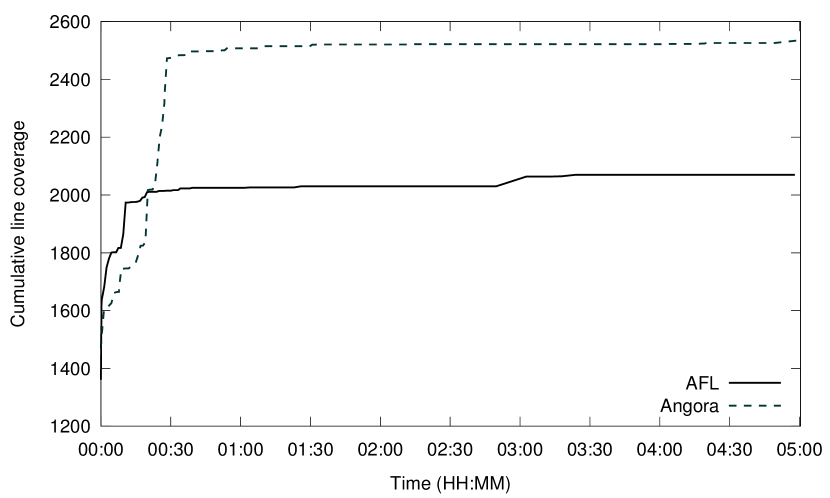
(a) Line coverage

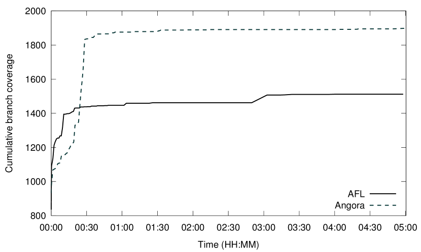
(b) Branch coverage

Figure 5: Line and branch coverage on file by d AFL in five hours

⬇

// readelf.c:620

if (namesz == 10 &&

strcmp((char*)&nbuf[noff], "DragonFly")==0

&& type == NT_DRAGONFLY_VERSION

&& descsz == 4) {

...

}

Figure 6: A complicated conditional statement in the file readelf.c in the program file whose true branch plored successfully but AFL could not

In the next sections, we will evaluate how each of key features contributes to its superior performance.

5.3 Context-sensitive branch count

5.3.1 Performance

Section 3.2 introduced context-sensitive branch count. We believe that distinguishing the same branch in different function call contexts will find more bugs. To evaluate this hypothesis, we ran file with context-sensitive branch count and context-insensitive branch count separately. Table VI shows that und 6 bugs with context-sensitive branch count, but no bug without it. Figure 7 shows that starting from 30 minutes into fuzzing, nsistently covered more cumulative lines with context-sensitive branch count. We discovered several real world examples where context-sensitive branch count allowed explore more paths. For example, Figure 8 shows a code snippet in the file readelf.c in the program file. The function getu32 is called in multiple contexts, and it returns different results based on the swap argument. Without context-sensitive branch count, uld not be able to explore both branches of the conditional statement in all calling contexts.

TABLE VI: Comparison of non-context-sensitive branch count vs.  context-sensitive branch count on the program file

Metric	Non-context-sensitive	Context-sensitive
Line coverage	$2416$	$2534$
Branch coverage	$1788$	$1899$
Unique crashes	$0$	$6$

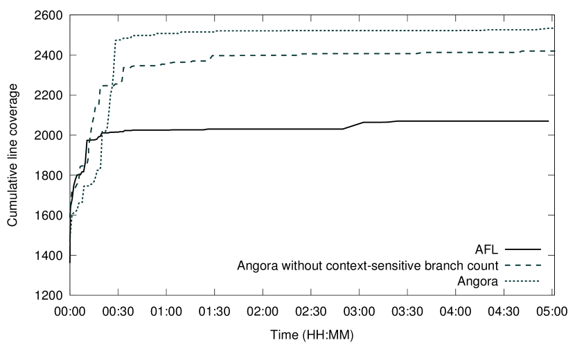
Figure 7: Comparison of non-context-sensitive vs. context-sensitive branch count on line coverage on the program file in five hours

⬇

// readelf.c:96

uint32_t getu32(int swap, uint32_t value) {

...

if (swap) {

...

return retval.ui;

} else

return value;

}

Figure 8: An example showing that without context sensitive branch count, uld not be able to explore both branches of the conditional statement, because getu32 is called from different contexts

5.3.2 Hash collision

Similar to AFL, ores branch counts in a hash table. When corporates calling context when counting branch coverage, it will insert more unique branches into the hash table, so we have to increase the size of the hash table to keep the collision rate low. We evaluated how many more unique branches context sensitivity brings on the real-world programs described in Section 5.2. The author of AFL observed that the number of unique branches (without context) usually ranges between 2k and 10k, and a hash table with $2^{16}$ buckets should be enough for common cases [30]. Table VII shows that incorporating context sensitivity increases the number of unique branches by a factor of at most 8, which requires us to increase the size of the hash table by also a factor of 8 to have the same expected hash collision rate. By default locates $2^{20}$ buckets in its hash table, which is 16 times as large as the hash table in AFL and should be adequate for most programs. Although growing the hash table may be harmful when it no longer fits in the cache, unlike AFL, which traverses the hash table both to find new paths and to prioritize inputs that cover many basic blocks, for each input averses the hash table only once to find new paths. Therefore, less affected by the growing size of the hash table, as demonstrated by the execution speed in Section 5.6).

TABLE VII: Impact of incorporating context sensitivity on unique branches

Program	Unique branches		Ratio
	Context insensitive	Context sensitive
file	$3578$	$13\,554$	$3.79$
jhead	$1049$	$6914$	$6.59$
xmlwf	$5531$	$11\,746$	$2.20$
djpeg	$3819$	$13\,787$	$3.61$
readpng	$7130$	$27\,577$	$3.87$
nm	$9029$	$65\,131$	$7.21$
objdump	$8113$	$40\,539$	$5.00$
size	$5964$	$40\,148$	$6.73$

5.4 Search based on gradient descent

Section 3.4 described how to use gradient descent to solve constraints in conditional statements. We compared gradient descent with two other strategies: random mutation, and VUzzer’s magic bytes plus random mutation. To exclude other variables in the measurement, we ensure that the three strategies receive the same inputs: we collected the inputs generated by AFL in Section 5.2, and fed them to the only inputs to fuzz. We ran r two hours using the above three strategies respectively.

Table VIII shows that gradient descent solved more constraints than the other two strategies on all the programs. As explained in the last paragraph of Section 5.1, the “magic bytes” strategy cannot solve constraints whose values are not copied directly from the input. For example, the variable descsz in Figure 6 is used in many constraints in the program, but it is not copied from the input directly, so the “magic bytes” strategy did not help.

TABLE VIII: Percentage of solved constraints in conditional statements using three strategies

Program	Random	Magic bytes	Gradient descent
		+ random
file	$63.5\text{\,}\mathrm{\char 37\relax}$	$76.0\text{\,}\mathrm{\char 37\relax}$	$87.1\text{\,}\mathrm{\char 37\relax}$
jhead	$86.9\text{\,}\mathrm{\char 37\relax}$	$87.1\text{\,}\mathrm{\char 37\relax}$	$97.6\text{\,}\mathrm{\char 37\relax}$
xmlwf	$77.4\text{\,}\mathrm{\char 37\relax}$	$81.4\text{\,}\mathrm{\char 37\relax}$	$97.0\text{\,}\mathrm{\char 37\relax}$
djpeg	$66.1\text{\,}\mathrm{\char 37\relax}$	$73.6\text{\,}\mathrm{\char 37\relax}$	$78.3\text{\,}\mathrm{\char 37\relax}$
readpng	$19.9\text{\,}\mathrm{\char 37\relax}$	$23.7\text{\,}\mathrm{\char 37\relax}$	$24.5\text{\,}\mathrm{\char 37\relax}$
nm	$57.5\text{\,}\mathrm{\char 37\relax}$	$66.4\text{\,}\mathrm{\char 37\relax}$	$80.2\text{\,}\mathrm{\char 37\relax}$
objdump	$47.0\text{\,}\mathrm{\char 37\relax}$	$54.9\text{\,}\mathrm{\char 37\relax}$	$56.3\text{\,}\mathrm{\char 37\relax}$
size	$44.1\text{\,}\mathrm{\char 37\relax}$	$52.4\text{\,}\mathrm{\char 37\relax}$	$54.3\text{\,}\mathrm{\char 37\relax}$

5.5 Input length exploration

TABLE IX: Comparison of input length exploration vs. other tools’ random strategy. The total columns report how many times the strategies created a longer input, respectively. The useful columns report how many of these inputs successfully explored new branches, respectively. The two rightmost columns report the average lengths of the inputs in the useful columns, respectively.

Program	Longer inputs				Average length
	Random				Random	missing
	Useful	Total	Useful	Total
file	185	79k	251	3342	889.9	399.0
jhead	0	66k	0	26	0.0	0.0
xmlwf	277	143k	588	2196	190.3	128.9
djpeg	32	106k	474	3476	846.6	283.6
readpng	46	35k	43	152	2242.7	363.1
nm	17	170k	19	872	771.7	248.0
objdump	44	214k	60	1614	1271.6	496.0
size	27	197k	33	1482	1584.5	949.7

Section 3.6 describes that creases the length of the input on demand when it observes that a path constraint may depend on the length, while AFL and related fuzzers increase the input length randomly. We compared these two strategies based on two criteria:

• How many times does the strategy increase the input length? Among the inputs created by this strategy, how many are useful? An input is useful if it explores a new branch either directly or after some mutation.

• What is the average length of those useful inputs?

We ran th our proposed strategy and the random strategy for five hours respectively. Section 5.5 shows that strategy increased the input length about two orders of magnitude fewer times than the random strategy, but it found more useful inputs in all cases except two: on readpng it found three fewer useful inputs out of a total of 46, and on jhead neither strategy found any useful input because jhead only parses the header of an image and therefore is not affected by the length of the image data. Section 5.5 also shows that while strategy generated more useful inputs, it generated shorter inputs on average on each program tested. Shorter inputs make many programs run faster. This evaluation shows that strategy generates higher quality inputs than the random strategy.

5.6 Execution speed

taint tracking is expensive. However, ns taint tracking once for each input, and then mutates the input and runs the program many times without taint tracking, so the one-time cost is amortized. Since branch count dominates the running time of the instrumented code without taint tracking, the nstrumented program runs at about the same speed as its AFL-instrumented version. Table X shows that AFL executes inputs at a slightly higher rate than owever, because nerates higher-quality inputs that more likely explore new branches, d much better coverage and found significantly more bugs as shown earlier.

TABLE X: Inputs tested per second

Program	AFL	file	971.17	791.73
jhead	2684.45	2648.91
xmlwf	2225.07	2206.24
djpeg	1439.94	1185.52
readpng	3374.43	2881.72
nm	1633.72	1045.35
objdump	1882.05	1192.04
size	1671.95	1174.55

6 Related work

6.1 Prioritize seed inputs

An important optimization for mutation-based fuzzers is to select the seed input wisely. Rebert et.al. [26] formulated and reasoned about the seed selection scheduling problem. They designed and evaluated six different seed selection algorithms based on PeachFuzzer [23]. The algorithms used different features to minimize the seed input set, such as execution time and file size. The result showed that heuristics employed by seed selection algorithms performed better than fully random sampling. AFLFast [4] observed that most fuzzing tests exercised the same few “high frequency” paths. They used Markov chain to identify “low-frequency” paths. AFLFast prioritized the inputs that contain such path. VUzzer [25] used control-flow features to model a path to prioritize the input whose path is hard-to-reach. Additionally, VUzzer detected error-handing basic-blocks, and prioritized the valid inputs that do not contain these basic-blocks. By contrast, lects the inputs whose paths contain conditional statements with unexplored branches. This is a more general strategy, which automatically directs focus on the low-frequency paths after exploring the high-frequency ones.

6.2 Taint-based fuzzing

Taint tracking has many uses, such as analyzing malware behavior [24], detecting and preventing information leaks [10, 29], and debugging software [22, 12]. It can also be used in fuzzing. Taint-based fuzzers analyze how an application processes an input to determine which part of the input should be modified. Some of these fuzzers [13, 2, 17] aimed to locate the values used in security sensitive code in input files, and then fuzzed these parts of input file to trigger crashes. For example, BuzzFuzz [13] used taint tracking to find which input bytes were processed by “attack point” that they defined. Dowser [17] considered code that likely leads to buffer overflow as security sensitive code. In other words, these fuzzers aimed to exploit bugs in the reachable paths. Woo et al. mentioned the trade off between exploration vs. exploitation [32]. n incorporate these techniques to exploit the explored paths. Taintscope [31] used taint analysis to infer checksum-handling code and bypassed these checks by control flow alteration, because these checks are hard to satisfy by mutating the input.

VUzzer [25] is an application-aware fuzzer that used taint analysis to locate the position of “magic bytes” in input files, and then assigned these magic bytes to fixed positions in the input. VUzzer can find magic bytes only when they appear continuously in the input. Steelix [19] improved VUzzer by learning from program state where the magic bytes are located in the input and how to mutate the input to match the magic bytes efficiently. By contrast, plies byte-level taint tracking to get the byte offsets in the input that flow into each conditional statement, and then mutates these bytes to satisfy the condition for the unexplored branch, so n find many more types of values efficiently than magic bytes, e.g., non-continuous magic bytes or magic bytes that are not copied directly from the input but are computed from the input. Besides, VUzzer uses a compressed bit-set data structure to represent taint labels where each bit corresponds to a unique byte offset in the input. Therefore, the size of the taint label is large for values with a complex pattern of input byte offsets because they can not be effectively compressed. By contrast, ores the byte offsets in a tree and uses indices into the tree as taint labels, so the size of the taint label is constant regardless of how many input byte offsets are in the label. For example, when the taint labels of several values have the same byte offsets, VUzzer repeatedly stores these byte offsets in each taint label, but ores these byte offsets only once in the tree, thus greatly reducing the memory consumption.

data structure for efficiently representing taint labels is similar to reduced ordered binary decision diagrams (roBDD). roBDD was used to represent dynamic slices [33] and data lineage [20] compactly, but to the best of our knowledge, the first to use this idea to represent taint labels efficiently.

6.3 Symbolic-assisted fuzzing

Dynamic symbolic execution provides high semantic insight into the target application. Since such techniques know how to trigger desired program state, they can be used to find vulnerabilities in programs directly. Classic approaches performed symbolic execution to maximize code coverage to find crashes [5, 8]. But the challenges of path explosion and constraint solving make symbolic execution hard to scale [6, 27]. Some tools tried to mitigate this obstacle by combining it with fuzzing [15, 16, 7, 28]. DART [15] and SAGE [16] used a dynamic symbolic execution engine to modify input in fuzzing. SYMFUZZ [7] leveraged symbolic analysis on an execution trace to detect dependencies among the bit positions in an input, and then used this dependency to compute an optimal mutation ratio to guide fuzzing. Driller [28] used dynamic symbolic execution only when fuzzing with AFL got stuck. However, all of them inherited the scalability problem from symbolic execution. By contrast, es not use symbolic execution, and can find many bugs on large programs efficiently.

7 Conclusion

We designed and implemented powerful mutation-based fuzzer that produces high quality inputs, thanks to the following key techniques: scalable byte-level taint tracking, context-sensitive branch count, search algorithm based on gradient descent, shape and type inference, and input length exploration. tperformed other state-of-the-art fuzzers by a wide margin. It found significantly more bugs than other fuzzers on LAVA-M, found 103 bugs that the LAVA authors could not trigger when they prepared the data set, and a total of 175 new bugs in eight popular, mature open source programs. Our evaluation shows that ised the bar of fuzzing to a new level.

8 Acknowledgment

We thank Dongyu Meng for helpful discussions throughout this project and for reviewing drafts of this paper. The paper improved substantially thanks to the detailed feedback from the anonymous reviewers.

TABLE III: IDs of bugs injected but unlisted by LAVA, because the LAVA authors were unable to trigger them when preparing the data set. und these bugs.

References

- [1] “American fuzzy lop” URL: http://lcamtuf.coredump.cx/afl/
- [2] Sofia Bekrar, Chaouki Bekrar, Roland Groz and Laurent Mounier “A taint based approach for smart fuzzing” In IEEE International Conference on Software Testing, Verification and Validation (ICST), 2012, pp. 818–825
- [3] “Binary fuzzing strategies: what works, what doesn’t” URL: https://lcamtuf.blogspot.sg/2014/08/binary-fuzzing-strategies-what-works.html
- [4] Marcel Böhme, Van-Thuan Pham and Abhik Roychoudhury “Coverage-based greybox fuzzing as markov chain” In Proceedings of the 2016 ACM SIGSAC Conference on Computer and Communications Security, 2016, pp. 1032–1043
- [5] Cristian Cadar, Daniel Dunbar and Dawson R Engler “KLEE: unassisted and automatic generation of high-Coverage tests for complex systems programs.” In OSDI 8, 2008, pp. 209–224
- [6] Cristian Cadar and Koushik Sen “Symbolic execution for software testing: three decades later” In Communications of the ACM 56.2, 2013, pp. 82–90
- [7] Sang Kil Cha, Maverick Woo and David Brumley “Program-adaptive mutational fuzzing” In Security and Privacy (SP), 2015 IEEE Symposium on, 2015, pp. 725–741
- [8] Sang Kil Cha, Thanassis Avgerinos, Alexandre Rebert and David Brumley “Unleashing mayhem on binary code” In Security and Privacy (SP), 2012 IEEE Symposium on, 2012, pp. 380–394
- [9] Brendan Dolan-Gavitt et al. “LAVA: large-scale automated vulnerability addition” In Security and Privacy (SP), 2016 IEEE Symposium on, 2016, pp. 110–121
- [10] William Enck et al. “TaintDroid: an information-flow tracking system for realtime privacy monitoring on smartphones” In ACM Transactions on Computer Systems (TOCS) 32.2, 2014, pp. 5
- [11] “Fuzzing with AFL is an art” URL: http://moyix.blogspot.com/2016/07/fuzzing-with-afl-is-an-art.html
- [12] Malay Ganai, Dongyoon Lee and Aarti Gupta “DTAM: dynamic taint analysis of multi-threaded programs for relevancy” In Proceedings of the ACM SIGSOFT 20th International Symposium on the Foundations of Software Engineering, 2012, pp. 46
- [13] Vijay Ganesh, Tim Leek and Martin Rinard “Taint-based directed whitebox fuzzing” In Proceedings of the 31st International Conference on Software Engineering, 2009, pp. 474–484
- [14] “gcov -— a test coverage program” URL: https://gcc.gnu.org/onlinedocs/gcc/Gcov.html#Gcov
- [15] Patrice Godefroid, Nils Klarlund and Koushik Sen “DART: directed automated random testing” In ACM SIGPLAN Notices 40.6, 2005, pp. 213–223
- [16] Patrice Godefroid, Michael Y Levin and David A Molnar “Automated whitebox fuzz testing.” In NDSS 8, 2008, pp. 151–166
- [17] Istvan Haller, Asia Slowinska, Matthias Neugschwandtner and Herbert Bos “Dowsing for overflows: a guided fuzzer to find buffer boundary violations.” In USENIX security, 2013, pp. 49–64
- [18] Chris Lattner and Vikram Adve “LLVM: a compilation framework for lifelong program analysis and transformation” In CGO, 2004, pp. 75–88
- [19] Yuekang Li et al. “Steelix: program-state based binary fuzzing” In Proceedings of the 2017 11th Joint Meeting on Foundations of Software Engineering, 2017, pp. 627–637
- [20] Zhiqiang Lin, Xiangyu Zhang and Dongyan Xu “Convicting exploitable software vulnerabilities: an efficient input provenance based approach” In Dependable Systems and Networks With FTCS and DCC, 2008. DSN 2008. IEEE International Conference on, 2008, pp. 247–256
- [21] “LLVM dataFlowSanitizer” URL: https://clang.llvm.org/docs/DataFlowSanitizer.html
- [22] Wes Masri, Andy Podgurski and David Leon “Detecting and debugging insecure information flows” In Software Reliability Engineering, 2004. ISSRE 2004. 15th International Symposium on, 2004, pp. 198–209
- [23] “Peach fuzzer” URL: http://www.peachfuzzer.com/
- [24] Georgios Portokalidis, Asia Slowinska and Herbert Bos “Argos: an emulator for fingerprinting zero-day attacks for advertised honeypots with automatic signature generation” In ACM SIGOPS Operating Systems Review 40.4, 2006, pp. 15–27
- [25] Sanjay Rawat et al. “VUzzer: application-aware evolutionary fuzzing” In NDSS, 2017
- [26] Alexandre Rebert et al. “Optimizing seed selection for fuzzing” In USENIX security, 2014, pp. 861–875
- [27] Yan Shoshitaishvili et al. “SOK:(State of) the art of war: offensive techniques in binary analysis” In Security and Privacy (SP), 2016 IEEE Symposium on, 2016, pp. 138–157
- [28] Nick Stephens et al. “Driller: augmenting fuzzing through selective symbolic execution” In Proceedings of the Network and Distributed System Security Symposium, 2016
- [29] Mingshen Sun, Tao Wei and John Lui “Taintart: a practical multi-level information-flow tracking system for android runtime” In Proceedings of the 2016 ACM SIGSAC Conference on Computer and Communications Security, 2016, pp. 331–342
- [30] “Technical "whitepaper" for afl-fuzz” URL: http://lcamtuf.coredump.cx/afl/technical_details.txt
- [31] Tielei Wang, Tao Wei, Guofei Gu and Wei Zou “TaintScope: a checksum-aware directed fuzzing tool for automatic software vulnerability detection” In Security and privacy (SP), 2010 IEEE symposium on, 2010, pp. 497–512
- [32] Maverick Woo, Sang Kil Cha, Samantha Gottlieb and David Brumley “Scheduling black-box mutational fuzzing” In Proceedings of the 2013 ACM SIGSAC conference on Computer & communications security, 2013, pp. 511–522
- [33] Xiangyu Zhang, Rajiv Gupta and Youtao Zhang “Efficient forward computation of dynamic slices using reduced ordered binary decision diagrams” In Proceedings of the 26th International Conference on Software Engineering, 2004, pp. 502–511