Power-law Interpolation of AC-DC Differences

Abstract

In this work we present a general method, commonly applied to the numerical analysis of stochastic models, to interpolate AC-DC differences (usually denoted by the greek letter $\delta$) between calibration points in thermal transfer standards. This method assigns a power-law behaviour to AC-DC differences, solely under the assumption that $\delta$ must be some smooth-varying function of voltage and frequency. We argue it may be straightfowardly applied to all working ranges of the standards, with no distinction.

I Introduction

Recent progress has been made towards the standardization of the AC voltage and current laiz2005 , but thermal transference methods, by which AC-volt and AC-ampère are compared to standard DC functions by thermal conversion, remain the most important resource in AC metrology practice on industrial and scientific electrical standards. The measurand is the difference between a DC current and the AC current needed to dissipate the same quantity $Q$ of heat on the transfer standard; it is usually called AC-DC difference, and denoted by the greek letter $\delta$ inglis1992 ; calibration .

We expect the measured AC-DC differences to be a continuous function of $Q$. Both numerical and theoretical results, and simple considerations on the physics of the heat production on the converters support this assumption. Neverthless, the same physical considerations are not yet able to make satisfactory predictions to a metrological level.

Despite this, we show in this work we can make use of the smoothness of $\delta$ (see Sec. IV), to associate correction exponents to the solution of the limiting equation for the problem, which is very easily formulated, and obtain a precise form for $\delta$, at least on some neighbouring frequencies and values of the input function cpem .

Sections II and III show results regarding the AC-DC difference in thermal converters, and review some important equations that relate to these results. Sections IV and V present a detailed description of the method, and some results obtained on transfer standards and thin-film multijunction systems; a brief conclusion is then presented in the last section.

II Thermal Converters

The most simple available thermal converter is the single junction thermal converter (SJTC), extensively studied and introduced as a transfer standard in the 50’s by Hermach hermach1952 . The SJTC may be combined with a resistor in order to extend its transfer ranges. This set makes a thermal converter (TC), which can be in series or parallel configuration, depending on the function being calibrated, whether it is voltage (when the set is assigned the term thermal voltage converter, or TVC) or current (alternatively, thermal current converter, or TCC), respectively.

A SJTC consists of a thermocouple welded to the middle of a low-resistence heater wire, through which electrical current flows and dissipate heat.The weld between thermocouple and heater is made from ceramic or similar material, and provides electrical, but no thermal insulation, allowing the hot junction to quickly get into thermal equilibrium with the center of the heater inglis1992 . These thermoelements, as they are also called, are usually mounted in an evacuated glass bulb, as shown in Fig. 1, and serve well to illustrate the principles of AC-DC metrology through thermal converters.

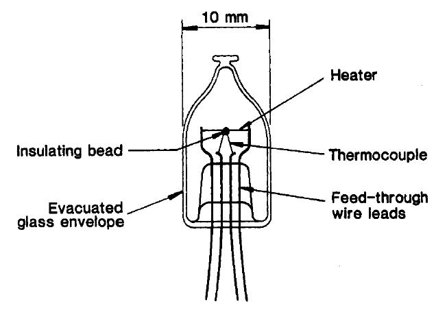
Figure 1: SJTC schematics. The temperature in the heater during operation is about $220^{o}C$, and its output voltage can range tipically from 8 to 12 mV; the bead provides electrical, but no thermal insulation, and allows the hot junction to quickly get into thermal equilibrium with the center of the heater. After Ref. inglis1992 .

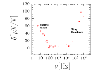
Figure 2: TVC/TCC characteristics sketch. This illustration shows a typical frequency behaviour of voltage AC-DC differences at fixed voltage, obtained from a rough simulation. The main causes of AC-DC difference in SJTC are DC offset, stray reactance and low-frequency thermal ripple.

Fig. 2 shows sketch of the typical frequency dependence of a SJTC, in which we can see the most relevant sources of error in thermal converters in general. The main causes of AC-DC difference in thermal converters are DC offset, stray reactance and low-frequency thermal ripple. The contribution of frequency combined effects to the AC-DC difference can be of the order of 0.1 $\mu$V/V from 100 Hz to 20 kHz, to 100 $\mu$V/V at 1 MHz for an ordinary SJTC sasaki1999 .

Thermal conversion is today the most economically feasible form available for making AC-DC transfers. Another very commonly used type of TC are eletronic, solid-state-based thermal standards as the one sketched in Fig. 3. The output of such an electronic TC responds linearly to temperature increases in a heater resistor. The output voltage at full input is about 2 V, instead of the 12 mV obtained from thermocouple-based TC’s calibration ; apnote .

Three electronic thermal standards Fluke model 792A (F792A), one of them assigned primary, are the transfer standards at Inmetro. And though studies are being carried out in order to replace them by thin-film multijunction converters (PMJTC) in primary standardization renato2009 , such electronic transfer standards are widely used in all areas where AC transfer is required, including many other National Metrology Institutes (NMI).

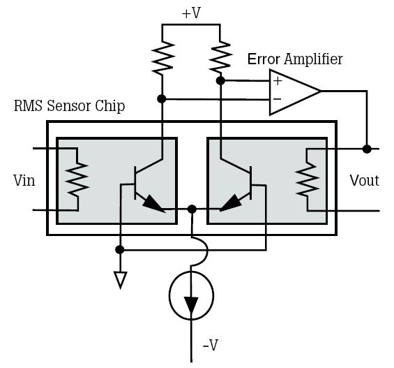
Figure 3: Simplified Fluke rms sensor. The sensor chip consists of two matched thermal voltage converters that lay on the temperature sensitivity of solid-state junctions rather than the ordinary thermocouple. After Ref. apnote .

III Transfer Characteristics

We can assign the output of a thermal converter the general form

$${E=kf[Y;\omega],}$$ (1)

where $E$ is the rms output voltage, $k$ is some constant scale factor dependent on the input funtion (voltage or current) and $f$ is a response functional dependent on the input function time evolution $Y$ and, by an obvious extension, the frequency $\omega$. The functional $f$ (which may be also called transfer characteristic) gives, without loss of generality, a measure of the heat dissipated in the heater of the TC, whatever design it might have, be it a simple resistive element or some complex electronic circuit.

May the input function $Y=I(t)$ be current, the AC-DC difference of a converter at some $I$ and $\omega$, referenced to a known DC current $I_{0}$, is given by schoe1978

$${\delta=-\left.{E[I]-E[I_{0}]\over n\cdot E[I_{0}]}\right|_{I=I_{0}}}$$ (2)

where $n$ is the characteristic exponent (often called “normalized index” or “linearity coefficient”) of the converter.

Should Joule effect be the only significant contribution to heat generation in the converter, supposing perfect sinewave voltage input $Y=I\sin(\omega t)$, we should have

$${f[Y]=\int_{\omega/2\pi}dt^{\prime}\cdot Y^{2}(t^{\prime}),}$$ (3)

and we expect $\displaystyle f[Y]\sim I^{2}$. As other thermoelectric effects become important, we must consider higher order contributions to $f$ in its arguments, or even incorporate time-dependent factors, if good estimates for AC-DC differences are to be obtained.

Then, following Schoenwetter schoe1978 , the lack of square-law response in SJTC for sinewave input currents at low-frequencies can be modelled as

$$\displaystyle{Y^{2}} {}={} \displaystyle{aI^{2}\left(1-m\cos(2\omega t)\right)}$$ (4)

$${+}\>\displaystyle{abI^{4}\left(1-m\cos(2\omega t)\right)^{2}}$$

where $a,b$ are scale constants, $I$ is the rms value of the current through the heater, $\tau$ is the thermal integration time constant of the TC and

$$m^{2}={1\over 1+\left(2\omega\tau\right)^{2}}.$$

Substituting Eq. 4 in Eq. 3 and carrying on the integration:

$${f[I]=I^{2}\left[\left({m^{2}\over 2}+1\right)bI^{2}+1\right]}$$ (5)

if $\omega\neq 0$. At DC regimes ($\omega=0$), the same procedure leads to

$${f[I_{0}]=I^{2}\left[bI^{2}+1\right].}$$ (6)

According to Ref. schoe1978 , $b$ can be evaluated through DC measurements of the output voltage of the TC. Then, applying Eqs. 5 and 6 to Eq. 2, the low-frequency AC-DC difference of a converter at some $I$ and $\omega$, referenced to a known DC standard $I_{0}$, is given by

$${\delta\approx-{bm^{2}\over 4}I^{2}.}$$ (7)

Eqs. 4 to 6 also enclose the following idea: losses and temperature-dependent coefficients in thermal and electrical conductivity of the heater increase with increasing input power, and affect the dissipated power in uneven ways at input signal maxima and minima. Eqs. 5 and 6 show that at low-frequency AC regimes, these non-linearities affect the average power generated in the sensor, in the sense that more AC than DC is required in order to obtain the same output response.

Eq. 7 was obtained by considering, as an aproximation, some time-independent transfer characteristic $f$, and a frequency-tracking correction to the input function of the form $1+m\cos(2\omega t)$, plus higher order terms that account for the non-linearities discussed above. The same aproximation also applies to F792A measurements calibration ; apnote , and is very similar, as far as the powers of $\nu$ and $V$ are concerned, to the results Hermach had earlier obtained hermach1952 , which account for radiation losses contributions as a perturbation to the heat-conduction equation above the thermal integration time-constant limit. Comments on the agreement of both results to PMJTC data can be found in Ref. laiz1999 .

These results bring, among many other implications, better knowledge of the expected limiting curves of $\delta$ at fixed voltage and frequency at low frequencies. This allows us to derive formulae for interpolation of AC-DC differences between calibration points.

Measurement of AC-DC differences in voltages and frequencies different from the ones usually offered in calibration services can be an important matter for data analysis and prediction, for instance. This brings the question as to whether it is possible to improve the results for standardization between calibration points of the standard, and has provided the initial motivation to this work.

IV Power-Law Interpolation

Based on the behaviour of the AC-DC difference $\delta$ reported in the previous sections, we expect, as $\nu\to 0$, that

$${\delta\sim{Y^{2}\over\nu^{2}}}$$ (8)

but for a multiplicative constant.

Assuming Eq. 8 holds, a common way to interpolate $(\nu,\delta)$ or $(Y,\delta)$ pairs to experimental AC-DC difference data is to operate a change of variables so as to make $\delta$ linear in its arguments; in few words, this means we pick $Y^{2}$ and $1/\nu^{2}$ as parameters. This change of variables is reported in Ref. 792apendixc .

Such linearization processes are based on some truncated integer-power expansion of $f$ in its arguments, true only in the limit. Deviations of Eq. 8 can be particularly important where uncertainties are of the order of the interpolation error estimates. And while this is not always true for the F792A, it certainly applies to PMJTC standards.

Our proposal is to neglect complex details as the limiting form of $f$ or the random effects of fluctuations, while still considering the possible strong higher order terms mentioned earlier, by assuming, in some neighborhood of the point to be interpolated, low-frequency $\delta$ has the power-law form

$${\delta\sim{Y^{2-\beta}\over\nu^{2-\alpha}}}$$ (9)

where $\alpha$ and $\beta$ are the corrections to the limiting form in Eq. 8.

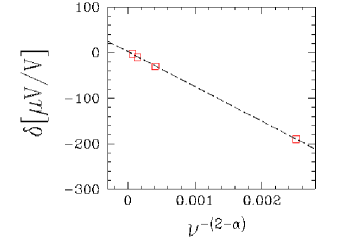
Figure 4: Linear fits of 792A data at fixed voltage. The picture shows a least square fit line for 792A AC-DC differences $\delta$ (in $\mu$V/V) at fixed 300 mV, and frequencies $10<\nu<40$ Hz. Uncertainties are of order of 10 $\mu$V/V, and are not shown.

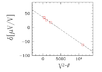
Figure 5: Linear fits of 792A data at fixed frequency. The picture shows a least square fit line for 792A AC-DC differences $\delta$ (in $\mu$V/V) at fixed 40 Hz, and voltages $0.002<V<0.020$ volts. Uncertainties range from 35 to 75 $\mu$V/V, and are not shown.

Exponents $\alpha$ and $\beta$ are adjusted under the condition of maximum linear correlation between, for instance, fixed-voltage or fixed-frequency AC-DC differences; this criterion has been consistently applied in similar adjustment on the context of scaling random systems fabio2001 . The implicit assumption behind Eq. 9 is that the AC-DC difference is a smooth function of $Y$ and $\nu$, in the statistical sense.

Table 1: Frequency Interpolation of F792A Data at 0.300 V

$\nu$	$\delta$	U	$\Delta$
10	-190	10	0.03
20	-30	10	0
30	-10	10	-0.60
40	-3	10	0.60

[2in][c] This table shows the adjusted points $(\nu,\delta)$, their combined uncertainties $U$ and the interpolation errors $\Delta$ for F792A calibration data. The frequency $\nu$ is given in hertz; $\delta$, $U$ and $\Delta$ are expressed in $\mu V/V$.

Table 2: Voltage Interpolation of F792A Data at 40 Hz

$V$	$\delta$	U	$\Delta$
0.002	-62	75	-0.28
0.006	18	60	0.27
0.010	26	50	-1.87
0.020	35	35	1.44

[2in][c] This table shows the adjusted points $(V,\delta)$, their combined uncertainties $U$ and the interpolation errors $\Delta$ for F792A calibration data. The voltage $V$ is given in volts; $\delta$, $U$ and $\Delta$ are expressed in $\mu V/V$.

Figs. 4 and 5 show least square fits for AC-DC low-frequency differences on two different F792A instruments, obtained from calibration against PMTC, both in voltage and frequency. Exponents $\alpha$ and $\beta$ were adjusted until the correlation coefficient $R^{2}$ of the fits came to a maximum. In Fig. 4, $\alpha=-0.6$ to $R^{2}=0.99998$; in Fig. 5, $\beta=3.5$ to $R^{2}=0.9995$ (see Eq. 9).

The combined uncertainties $U$ are of 10 $\mu$V/V for the points in Fig. 4; for the points in Fig. 5, $U$ range from 35 to 75 $\mu$V/V. The standard errors of the fits are $\sigma=0.6$ $\mu$V/V (Fig. 4) and $\sigma=1.7$ $\mu$V/V (Fig. 5). These figures represent negligible contribution to the combined uncertainties of those points, and therefore no important contribution of the interpolation method to the uncertainty is expected in points interpolated between calibration points. The adjusted points $(\nu,\delta)$ and $(V,\delta)$, their combined uncertainties $U$ and the interpolation errors $\Delta$ are summarized in Tables 1 and 2.

V Results for PMJTC Data

The AC standardization project at Inmetro has a fully operational automated PMJTC voltage system, and the first measurements are being carried out. This system is composed of two 180 $\Omega$-heater PMJTC, calibrated at Physikalisch-Technische Bundesanstalt (PTB), in 1.5 volts and frequencies from 10 to 1 MHz; twelve 90 $\Omega$, one 400 $\Omega$ and one 900 $\Omega$ PMJTC. These junctions are used with range-resistors from 200 mV to 1000 V; the standardization method chosen is the voltage step-up renato2009 .

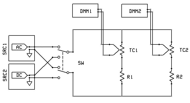
Figure 6: PMJTC system at Inmetro. This sketch shows the voltage system used to calibrate junctions in 50 V. SRC1 and SRC2 are multifunction calibrators; SW is a switch; DMM1 and DMM2 are digital nanovoltmeters; TC1/R1 and TC2/R2 are sets of PMJTC and range resistors (see text).

Fig. 6 shows an schematics of the PMJTC voltage system used at Inmetro to calibrate junctions from 1.5 to 100 V. In this sketch, SRC1 and SRC2 are multifunction calibrators Fluke model 5720; SW is an AC-DC switching unit built at the Swiss Federal Office of Metrology and Accreditation (Metas); DMM1 and DMM2 are digital nanovoltmeters Keithley model 2182A; TC1 and TC2 are PMJTC made at PTB; and R1 and R2 are the proper range resistors for the set.

We assume Eq. 9 holds, and again adjust exponents $\alpha$ and $\beta$ under the condition of maximum linear correlation between AC-DC differences. Figs. 7 and 8 show frequency fits for AC-DC low-frequency differences on two different 90 $\Omega$ PMJTC sets, obtained from calibration against the 90 $\Omega$ standards for the 50 V step. Exponents $\alpha$ were adjusted until the correlation coefficient $R^{2}$ of the fits came to a maximum. In Fig. 7, $\alpha=-1.1$ to $R^{2}=0.893$; in Fig. 8, $\alpha=0.5$ to $R^{2}=0.807$ (see Eq. 9).

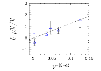
Figure 7: Linear fits of PMJTC data at fixed voltage (1). The picture shows a least square fit of AC-DC differences $\delta$ (in $\mu$V/V) for the 90 $\Omega$ PMJTC set 90-8/R100V at fixed 50 V, and frequencies $10<\nu<1000$ Hz. Error bars are standard deviations, and range from 0.2 to 0.7 $\mu$V/V.

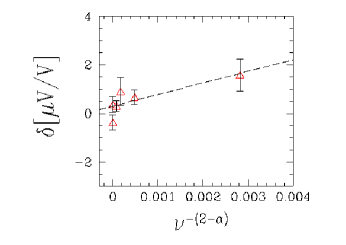
Figure 8: Linear fits of PMJTC data at fixed voltage (2). The picture shows a least square fit of AC-DC differences $\delta$ (in $\mu$V/V) for the 90 $\Omega$ PMJTC set 90-9/R300V at fixed 50 V, and frequencies $10<\nu<1000$ Hz. Error bars are standard deviations, and range from 0.4 to 0.7 $\mu$V/V.

The standard deviations $s$ of the AC-DC difference measurements range from 0.2 to 0.7 $\mu$V/V for the points in Fig. 7; for the points in Fig. 8, $s$ range from 0.4 to 0.7 $\mu$V/V. The standard errors of the fits are $\sigma=0.33$ $\mu$V/V (Fig. 7) and $\sigma=0.15$ $\mu$V/V (Fig. 8). These figures are of the order of the standard deviations of the measurements, and must represent no significant contribution to the combined uncertainties of those points, and therefore no important contribution of the interpolation method to the uncertainty is expected in points interpolated between calibration points. The adjusted points $(\nu,\delta)$, the standard deviations $s$ and the interpolation errors $\Delta$ are summarized in Tables 3 and 4.

Table 3: Frequency Interpolation of PMJTC Data at 50 V (1)

$\nu$	$\delta$	s	$\Delta$
10	1.58	0.66	0.01
20	0.67	0.30	-0.16
30	0.90	0.57	-0.33
40	0.31	0.22	-0.13
500	-0.37	0.31	-0.40
1000	0.36	0.33	0.35

[2in][c] This table shows the adjusted points $(\nu,\delta)$, their combined uncertainties $U$ and the interpolation errors $\Delta$ for PMJTC set labelled 90-8/R100V. The frequency $\nu$ is given in hertz; $\delta$, $U$ and $\Delta$ are expressed in $\mu V/V$.

Table 4: Frequency Interpolation of PMJTC Data at 50 V (2)

$\nu$	$\delta$	s	$\Delta$
10	3.11	0.46	-0.01
20	-0.62	0.41	0.16
30	-1.46	0.65	-0.16
40	-1.60	0.50	-0.16
500	-1.53	0.49	0.05
1000	-1.46	0.55	0.12

[2in][c] This table shows the adjusted points $(\nu,\delta)$, their combined uncertainties $U$ and the interpolation errors $\Delta$ for PMJTC set labelled 90-9/R300V. The frequency $\nu$ is given in hertz; $\delta$, $U$ and $\Delta$ are expressed in $\mu V/V$.

VI Final Remarks

Fully- and semi-automated systems based on electronic thermal standards can make it very practical for laboratories to handle demands for large numbers of calibration points in many different ranges. Recently reported automated systems have overall calibration time limited only by the charge duration of embedded batteries bob , and though AC-DC transfer services can often last a few weeks long, electronic thermal standards are very likely to be around for a long time yet. So, one of the many features of good interpolation methods is a possible reduction on the number of calibrated points within ranges of electronic standards such as the F792A, both in voltage and frequency.

The method presented here has never been applied to the study of measurement data from TC, though it can be very useful in the analysis of many theoretical models of statistical physics fabio2001 ; eu2007 . As in those models, further investigation of the correction exponents (Eq. 9) for PMJTC data can bring deeper understanding of these non-linearities and might lead to important insights on these effects, instead of the other way around.

We also obtained small interpolation uncertainties on PMJTC standards. For PMJTC, a robust interpolation method, which in some way takes into account the physics behind the measurement system, together with calibration schemes such as described in youlden1963 , can help to spare the extensive use of standards, while still promoting improvement in results.

We should expect deviations from square and inverse-square laws that rule AC-DC differences at low frequencies in such standards to be related mainly to Thomsom heating and non-linear contributions to emissivity and thermal diffusivity in the heater hermach1952 ; inglis1992 ; sasaki1999 ; laiz1999 ; oldham1997 , as well as non-linear contributions from circuitry in electronic standards, though the contribution of sistematic fluctuations of statistical nature should also be investigated.

References

- (1) Laiz,H., “Low Frequency AC Voltage Standards: An Overview”, in Proc. of VI SEMETRO, pp. 15 (2005)
- (2) Inglis, B. D., “Standards for AC-DC Transfer”, Metrologia 29, 191 (1992)
- (3) Fluke Corp., Calibration: Phylosophy in Practice, Fluke Corp. (1994)
- (4) F. A. Silveira, R. M. Souza. and R. P. Landim, “Power-Law Picture for the Interpolation of AC-DC Differences in Thermal Standards”, Digest of Conf. on Precision Electromagnetic Measurements (CPEM2010), June 13- June 18, 2010, Daejeon, Korea.
- (5) Hermach, F. L., “Thermal Converters as AC-DC Transfer Standards for Current and Voltage Measurements at Audio Frequencies”, J. Res. Nat. Bur. Std. 48, 163 (1952)
- (6) Sasaki, H. and Takahashi, K., “Development of a High Precision AC-DC Transfer Standard using FRDC Method”, Res. of Electr. Lab. 989, 90P (1999)
- (7) Fluke Corp., Design and Evaluation of the 792A AC/DC Transfer Standard, Fluke Application Note 1268781 A-ENG-N Rev. B (2000)
- (8) Afonso Jr., R., Borghi, G., Landim, R. P., Afonso, E. and Silveira, F. A., “O Sistema de Padronização AC do Inmetro”, in Proc. of VII Semetro, N 52010 (2009)
- (9) Schoenwetter, H. K., “An RMS Digital Voltmeter/Calibratior for Very-Low Frequencies”, IEEE Trans. Instr. Meas. 27, 259 (1978)
- (10) Laiz, M. L., “Low Frequency Behaviour of Thin-Film Multijunction Thermal Converters”, Physikalisch-Technische Bundesanstalt, PTB-Bericht E-63 (1999)
- (11) Fluke Corp., Calculating Correction Factors for F100 Hz, 792A Transfer Standard Instruction Manual, PN 871723 Rev 1, C-1 (1990)
- (12) Aarão Reis, F. D. A., “Universality and Corrections to Scaling in the Ballistic Deposition Model”, Phys. Rev. E 63, 056116 (2001)
- (13) Oldham, N. M., Svetlana, A.-Z. and Parker, M. E., “Exploring the Low-Frequency Performance of Thermal Converters Using Circuit Models and a Digitally Synthesized Source”, IEEE Trans. Instr. Meas. 46, 352 (1997)
- (14) Silveira, F. A. and Aarão Reis, F. D. A.,“Surface and Bulk Properties of Deposits Grown With a Bidisperse Ballistic Deposition Model”, Phys. Rev. E 75, 061608 (2007)
- (15) Teixeira, V. M., Ventura, R. V. F., Souza, R. M., Afonso Jr., R., Landim, R. P. and Afonso, E., “Moving Towards Full Automation of High Accuracy Multifunction Instruments Calibration Systems”, in Proc. of VIII Semetro, N 52343 (2009)
- (16) Youlden, W. J., “Measurement Agreement Comparisons”, in Precision Measurement and Calibration: Statistical Concepts and Procedures, Ed. H. H. Ku, NBS Special Publication 300 vol 1, 146 (1963)