4D Gauge Theories with Conformal Matter

Abstract

One of the hallmarks of 6D superconformal field theories (SCFTs) is that on a partial tensor branch, all known theories resemble quiver gauge theories with links comprised of 6D conformal matter, a generalization of weakly coupled hypermultiplets. In this paper we construct 4D quiverlike gauge theories in which the links are obtained from compactifications of 6D conformal matter on Riemann surfaces with flavor symmetry fluxes. This includes generalizations of super QCD with exceptional gauge groups and quarks replaced by 4D conformal matter. Just as in super QCD, we find evidence for a conformal window as well as confining gauge group factors depending on the total amount of matter. We also present F-theory realizations of these field theories via elliptically fibered Calabi-Yau fourfolds. Gauge groups (and flavor symmetries) come from 7-branes wrapped on surfaces, conformal matter localizes at the intersection of pairs of 7-branes, and Yukawas between 4D conformal matter localize at points coming from triple intersections of 7-branes. Quantum corrections can also modify the classical moduli space of the F-theory model, matching expectations from effective field theory.

1 Introduction

In addition to providing the only consistent theory of quantum gravity, string theory also predicts the existence of qualitatively new quantum field theories. A notable example of this kind is the construction of conformal field theories in six spacetime dimensions. These quantum field theories are intrinsically strongly coupled, and the only known way to generate examples is via compactifications of string theory backgrounds with six flat spacetime dimensions [1, 2, 3, 4] (for a partial list of references, see e.g. [5, 6, 7, 8, 9, 10, 11, 12, 13, 14] as well as [15, 16, 17, 18, 19, 20, 21, 22, 23, 24, 25, 26, 27, 28, 29, 30, 31, 32, 33, 34, 35, 36, 37, 38, 39, 40, 41, 42, 43, 44, 45, 46, 47, 48, 49, 50, 51, 52, 53, 54, 55, 56, 57]). Moreover, many impenetrable issues in strongly coupled phases of lower-dimensional systems lift to transparent explanations in the higher-dimensional setting.

This paradigm has had great success in theories with eight or more real supercharges. Intuitively, the reason for this is that with so much supersymmetry, the resulting quantum dynamics – while still interesting – is tightly constrained. For example, in the context of 4D $\mathcal{N}=2$ gauge theories, the metric on the Coulomb branch moduli space is controlled by derivatives of the pre-potential, a holomorphic quantity, as used for example, in [58, 59]. Even with reduced supersymmetry, holomorphy is still an invaluable guide [60], but many quantities now receive quantum corrections.

One particularly powerful way to construct and study many features of strongly coupled field theories in four and fewer dimensions is to first begin with a higher-dimensional field theory, and compactify to lower dimensions. For example, compactification of the $\mathcal{N}=(2,0)$ 6D SCFTs on a $T^{2}$ leads to a geometric characterization of S-duality in $\mathcal{N}=4$ Super Yang-Mills theory [61], and analogous $\mathcal{N}=2$ dualities follow from compactification on more general Riemann surfaces [62, 63]. The extension to the vast class of new $\mathcal{N}=(1,0)$ 6D SCFTs constructed and classified in references [15, 17, 19, 23] (see also [22, 64]) has only recently started to be investigated, but significant progress has already been made in understanding the underlying 4D theories obtained from compactifying special choices of $\mathcal{N}=(1,0)$ 6D SCFTs on various manifolds. For a partial list of references to compactifications of 6D SCFTs, see e.g. [25, 26, 28, 34, 35, 39, 46, 47, 48, 50, 53, 55, 56, 65].

In this paper we construct generalizations of 4D $\mathcal{N}=1$ quiver gauge theories in which the role of the links are played by compactifications of 6D conformal matter on a Riemann surface. To realize a quiver, we shall weakly gauge flavor symmetries of these matter sectors by introducing corresponding 4D $\mathcal{N}=1$ vector multiplets. Additional interaction terms such as generalized Yukawa couplings can also be introduced by gluing together neighboring cylindrical neighborhoods of 6D conformal matter. Depending on the number of matter fields, and the types of interaction terms which have been switched on, we can expect a number of different possibilities for the infrared dynamics of these generalized quivers.

Even the simplest theory of this kind, namely a generalization of SQCD with 4D conformal matter turns out to have surprisingly rich dynamics. First of all, we can consider a wide variety of 4D conformal matter sectors depending on the choice of punctured Riemann surface and background flavor symmetry fluxes. Weakly gauging a common flavor symmetry for many such sectors then leads us to a generalization of SQCD with 4D conformal matter. It is natural to ask whether this SQCD-like theory flows to an interacting fixed point. To address this, we first note that if weakly gauge the flavor symmetry of conformal matter, we can compute the beta function coefficient for the gauge coupling via anomalies. It is summarized schematically by the formula:

$$b_{G}=3h_{G}^{\vee}-b^{\mathrm{matter}}_{G},$$ (1.1)

where $h_{G}^{\vee}$ is the dual Coxeter number of the gauge group $G$. In the simplest case where we compactify 6D conformal matter with flavor symmetry $G\times G$ on a $T^{2}$ with no fluxes, it is well-known that we obtain a 4D $\mathcal{N}=2$ SCFT [26, 28, 34]. Weakly gauging a common $G$ for $n$ such 4D conformal matter sectors produces a 4D $\mathcal{N}=1$ gauge theory with flavor symmetry $G^{n}$ in the ultraviolet. For $n=3$, we are at the top of the conformal window, $n=2$ also produces an SCFT, and $n=1$ is outside the conformal window, instead producing a confining gauge theory with a deformed quantum moduli space. Generalizations of this construction to 4D conformal matter on genus $g$ Riemann surfaces with fluxes from flavor symmetries produce additional examples of generalized SQCD theories. Since we can calculate the contribution from each such matter sector to the weakly gauged flavor symmetry, we can see clear parallels with the conformal window of SQCD with gauge group $SU(N_{c})$ and $N_{f}$ flavors [60]:

$$\frac{3}{2}N_{c}<N_{f}<3N_{c}.$$ (1.2)

where in the present case we have:

$$\frac{3}{2}h_{G}^{\vee}\lesssim b^{\mathrm{matter}}_{G}\leq 3h_{G}^{\vee}.$$ (1.3)

The upper bound is sharp, since we can explicitly present examples which saturate the bound. The lower bound appears to depend in a delicate way on the curvature of the punctured Riemann surface and flavor symmetry fluxes. Note also that in contrast to ordinary SQCD, we expect an interacting fixed point at both the top and bottom of the window. The reason is simply that the 4D conformal matter is itself an interacting fixed point.

Starting from this basic unit, we can construct elaborate networks of theories by gauging additional flavor symmetry factors, producing a tree-like graph of quiver gauge theories. We can also introduce the analog of Yukawa couplings for conformal matter, though the field theory interpretation of this case is particularly subtle.

To address this and related questions, it is helpful to use the UV complete framework of string theory. Indeed, our other aim in this work will be to engineer examples of these theories using F-theory on elliptically fibered Calabi-Yau fourfolds. The philosophy here is rather similar to the approach taken in the F-theory GUT model building literature [66, 67] (see [68, 69] for reviews), namely we consider degenerations of the elliptic fibration over a complex surface (codimension one in the base) to generate our gauge groups, degenerations over complex curves (codimension two in the base) to generate 4D conformal matter, and degenerations at points (codimension three in the base) to generate interaction terms between conformal matter sectors. A common theme in this respect is that the presence of singularities will mean that to make sense of the Calabi-Yau geometry, we must perform blowups and small resolutions in the base. In the context of 6D conformal matter from F-theory on an elliptically fibered Calabi-Yau threefold, this is by now a standard story, namely we introduce additional $\mathbb{P}^{1}$’s in the corresponding twofold base [9, 15, 70]. For 4D models, the presence of codimension three singularities in the base necessitates introducing compact collapsing surfaces.

Geometrically, then, we expect to obtain a rich set of canonical singularities associated with the presence of collapsing surfaces and curves in the threefold base. In higher dimensions, this is actually the main way to generate examples of 6D SCFTs. In four dimensions, however, there can and will be quantum corrections to the classical moduli space. This is quite clear in the F-theory description since Euclidean D3-branes can wrap these collapsing surfaces. This means there will be instanton corrections which mix the Kähler and complex structure moduli of the compactification.

To track when we can expect such quantum corrections to be present, it is helpful to combine top down and bottom up considerations. Doing so, we show that in some cases, a putative 4D SCFT generated from a Calabi-Yau fourfold on a canonical singularity instead flows to a confining phase in the infrared. We also present some examples which realize 4D SCFTs. All of this indicates a new arena for engineering strong coupling phenomena in 4D theories.

The rest of this paper is organized as follows. In section 2 we briefly review some elements of 6D conformal matter and its compactification to 4D conformal matter. We then introduce the general method of construction for generating 4D gauge theories with conformal matter. Section 3 focusses on generalizations of SQCD in which the matter fields are replaced by 4D conformal matter. In particular, we show there is a conformal window for our gauge theories, and also analyze the dynamics of these theories below the conformal window. We also present in section 4 some straightforward generalizations based on networks of SQCD-like theories obtained from gauging common flavor symmetries. With this field theoretic analysis in hand, in section 5 we next turn to a top down construction of this and related models via compactifications of F-theory. Proceeding by codimension, we show how various configurations of 7-branes realize and extend these field theoretic considerations. The field theory analysis also indicates that the classical moduli space of the F-theory model is in many cases modified by quantum corrections, which we also characterize. We present our conclusions in section 6. Some additional details on singularities in F-theory models as well as details on conformal matter for various SQCD-like theories are presented in the Appendices.

2 6D and 4D Conformal Matter

In this section we present a brief review of 6D conformal matter, and its compactification on a complex curve. Our aim will be to use compactifications of this theory as our basic building block in realizing a vast array of strongly coupled 4D $\mathcal{N}=1$ quantum field theories.

From the perspective of string theory, there are various ways to engineer 6D SCFTs. For example, theories of class $\mathcal{S}_{\Gamma}$ admit a description in both M-theory and F-theory [17]. In M-theory, they arise from a stack of $N$ M5-branes probing an ADE singularity $\mathbb{C}^{2}/\Gamma_{ADE}$ in the transverse geometry $\mathbb{R}_{\bot}\times\mathbb{C}^{2}/\Gamma_{ADE}$. We can move to a partial tensor branch by keeping each M5-brane at the orbifold singularity and separating them along the $\mathbb{R}_{\bot}$ direction. Doing so, we obtain a 7D Super Yang-Mills theory of gauge group $G_{ADE}$ for each compact interval separating neighboring M5-branes. The M5-branes have additional edge modes localized on their worldvolume. The low energy limit is a 6D quiver gauge theory with 6D conformal matter localized on the M5-branes. In F-theory, each of these gauge group factors is realized in F-theory by a compact $-2$ curve in a twofold base and is wrapped by a 7-brane of gauge group $G_{ADE}$. Collisions of 7-branes at points of the geometry lead to additional singular behavior for the elliptic fibration, namely the location of 6D conformal matter. The F-theory picture is particularly helpful because it provides a systematic way to determine the tensor branch moduli space. Essentially, we keep performing blowups of collisions of 7-branes until all fibers on curves are in Kodaira-Tate form. Said differently, in the Weierstrass model:

$$y^{2}=x^{3}+fx+g,$$ (2.1)

we seek out points where the multiplicity $f$, $g$ and $\Delta=4f^{3}+27g^{2}$ is equal to or higher than $(4,6,12)$ (see Appendix A). The presence of such points is resolved by performing a sequence of blowups in the base to proceed to the tensor branch. As illustrative examples, the case of a single M5-brane probing an E-type singularity is realized by the singular Weierstrass models:

$$(E_{6},E_{6}) \text{:}\text{ \ \ }y^{2}=x^{3}+u^{4}v^{4}$$ (2.2)

$$(E_{7},E_{7}) \text{:}\text{ \ \ }y^{2}=x^{3}+u^{3}v^{3}x$$ (2.3)

$$(E_{8},E_{8}) \text{:}\text{ \ \ }y^{2}=x^{3}+u^{5}v^{5}.$$ (2.4)

Another important feature of such constructions is that the anomaly polynomial for background global symmetries can be computed for all such 6D SCFTs [71]. The general structure of the anomaly polynomial is a formal degree eight characteristic class:

$$I_{8}= \alpha c_{2}(R_{6D})^{2}+\beta c_{2}(R_{6D})p_{1}(T)+\gamma p_{1}(T)^{2}+\delta p_{2}(T)$$ (2.5)

$$+\sum_{i}\left[\omega_{i}\,\frac{\mathrm{tr}_{\rm fund}F_{i}^{4}}{16}+\nu_{i}\left(\,\frac{\mathrm{Tr}F_{i}^{2}}{4}\right)^{2}+\,\frac{\mathrm{Tr}F_{i}^{2}}{4}\left(\kappa_{i}p_{1}(T)+\xi_{i}c_{2}(R)+\sum_{j}\chi_{ij}\,\mathrm{Tr}F_{j}^{2}\right)\right]$$

where here, $R_{6D}$ refers to the $SU(2)$ R-symmetry bundle, $T$ the tangent bundle, and the $F_{i}$ refer to possible flavor symmetries of the 6D SCFTs.

Starting from these 6D theories, we reach a wide variety of lower-dimensional systems by compactifying on a Riemann surface. This can also be accompanied by activating various abelian background fluxes, as well as holonomies of the non-abelian symmetries [39, 47, 65].

The F-theory realization of 4D field theories involves working with an elliptically fibered Calabi-Yau fourfold with $\mathcal{B}$ a non-compact threefold base. In F-theory terms, we can engineer examples of 6D conformal matter on a curve by taking $\mathcal{B}$ to be given by a complex curve $\Sigma_{g}$ of genus $g$ and a rank two vector bundle $\mathcal{V}\rightarrow\Sigma_{g}$ so that the total space is a threefold. A particularly tractable case to analyze is where $\mathcal{V}$ is a sum of two line bundles $\mathcal{L}_{1}\oplus\mathcal{L}_{2}$ of respective degrees $d_{1}$ and $d_{2}$ so that the base $\mathcal{B}$ is the total space $\mathcal{L}_{1}\oplus\mathcal{L}_{2}\rightarrow\Sigma_{g}$. Introducing local coordinates $(u_{1},u_{2},v)$ for the line bundle directions and the Riemann surface, we can expand the Weierstrass coefficients $f$ and $g$ as polynomials in these local coordinates:

$$f=\underset{i,j}{\sum}f_{ij}(v)(u_{1})^{i}(u_{2})^{j}\text{, \ \ }g=\underset{i,j}{\sum}g_{ij}(v)(u_{1})^{i}(u_{2})^{j}.$$ (2.6)

In general, we can consider geometries in which there are various 7-brane intersections over curves and points of the base. One way to further constrain the profile of intersections so that the only intersection available takes place over the curve $\Sigma_{g}$ is to enforce the condition that $\mathcal{B}$ is a local Calabi-Yau threefold, which in turn requires $d_{1}+d_{2}+(2-2g)=0$. Doing so, the coefficients $f_{ij}$ and $g_{ij}$ can be constant, and we automatically engineer conformal matter compactified on a genus $g$ curve. Switching on background fluxes through the 7-branes then engineers in F-theory the field theoretic constructions presented in the literature [39, 47, 48, 53, 65].

Regardless of how we engineer these examples, it should be clear that even this simple class of examples leads us to a rich class of 4D theories which we shall refer to as 4D conformal matter. Indeed, in most cases there is strong evidence that these theories flow to an interacting fixed point.

For example, we can, in many cases, calculate the anomalies of the 4D theory by integrating the anomaly polynomial of the 6D theory over the Riemann surface [72]. Then, the principle of a-maximization [73] yields a self-consistent answer for the infrared R-symmetry for the putative SCFT. As standard in this sort of analysis, we assume the absence of emergent $U(1)$ symmetries in the infrared. In some limited cases, the procedure just indicated is inadequate for determining the anomalies of the resulting 4D theory. When the degree of the flavor flux is too low [47], (typically when the Chern class is one), or when the Riemann surface has genus one [26, 34], then alternative methods must be used to determine the anomalies of the 4D theory.

A case of this type which will play a prominent role in our analysis of SQCD-like theories is the theory obtained from compactification of rank one $(G,G)$ conformal matter on a $T^{2}$ with no flavor fluxes. In this case, we expect a 4D $\mathcal{N}=2$ SCFT with flavor symmetry $G\times G$. This 4D $\mathcal{N}=2$ conformal matter is a natural generalization of a hypermultiplet, but in which the “matter fields” are also an interacting fixed point.

3 $\mathcal{N}=1$ SQCD with Conformal Matter

In the previous section we observed that there is a natural generalization of ordinary matter obtained from compactifications of 6D conformal matter on complex curves. In these theories, there is often a non-abelian flavor symmetry. Our aim in this section will be to determine the field theory obtained from weakly gauging this flavor symmetry. For simplicity, in this section we focus on the special case of rank one $(G,G)$ 6D conformal matter compactified on a $T^{2}$ with no fluxes, namely 4D $\mathcal{N}=2$ conformal matter. We denote this theory by a link between two flavor symmetries:

$$[G]\overset{CM}{-}[G].$$ (3.1)

Before proceeding to the construction of SQCD-like theories, let us begin by listing some properties of this theory. First of all, the anomaly polynomial is given by (see Appendix for our conventions):

$$I_{6}= \frac{k_{RRR}}{6}c_{1}(R)^{3}-\frac{k_{R}}{24}p_{1}(T)c_{1}(R)+k_{RG_{L}G_{L}}\frac{\mathrm{Tr}(F^{2}_{G_{L}})}{4}c_{1}(R)+k_{RG_{R}G_{R}}\frac{\mathrm{Tr}(F^{2}_{G_{R}})}{4}c_{1}(R)+\ldots$$ (3.2)

where here $R$ is a $U(1)$ subalgebra of the R-symmetry of the 4D theory and $T$ is the formal tangent bundle, $F$ is the field strength of $G_{L}$ or $G_{R}$ flavor symmetries, and the dots indicate possible abelian flavor symmetries and mixed contributions. From this, we read off both the conformal anomalies $a$ and $c$,

$$a=\frac{9}{32}k_{RRR}-\frac{3}{32}k_{R}$$ (3.3)

$$c=\frac{9}{32}k_{RRR}-\frac{5}{32}k_{R}.$$ (3.4)

If we weakly gauge the flavor symmetries, the contribution to the beta function of the gauge coupling is set by the term in the anomaly polynomial of the 4D theory involving an R-current and two flavor currents, namely, the contribution as a matter sector is [74] (see also [72]):

$$b^{\mathrm{matter}}_{G}=\frac{3k_{RGG}}{2},$$ (3.5)

so that the numerator of the NSVZ beta function [75, 76, 77, 78] is:

$$b_{G}=3C_{2}(G)-b^{\mathrm{matter}}_{G}.$$ (3.6)

In what follows, it will be helpful to recall that in our conventions,

$$C_{2}(G)=h_{G}^{\vee},$$ (3.7)

with $h_{G}^{\vee}$ the dual Coxeter number of the group $G$.

For the $(G,G)$ 6D conformal matter compactified on a $T^{2}$ with no fluxes, $a,c$ and the contribution to the beta function coefficients are [26, 34]:

$$a=24\gamma-12\beta-18\delta,$$ (3.8a)

$$c=64\gamma-12\beta-8\delta,$$ (3.8b)

$$b^{\mathrm{matter}}_{L}=24\kappa_{L},$$ (3.8c)

$$b^{\mathrm{matter}}_{R}=24\kappa_{R},$$ (3.8d)

where, the coefficients $\beta,\gamma,\delta,\kappa_{L,R}$ can be read off from the 6D anomaly polynomial of rank one $(G,G)$ conformal matter theories

$$I_{8}=\alpha c_{2}(R_{6D})^{2}+\beta c_{2}(R_{6D})p_{1}(T)+\gamma p_{1}(T)^{2}+\delta p_{2}(T)+\kappa_{L}p_{1}(T)\frac{\mathrm{Tr}(F_{L}^{2})}{4}+\kappa_{R}p_{1}(T)\frac{\mathrm{Tr}(F_{R}^{2})}{4}+\ldots$$ (3.9)

and the explicit values for the coefficients are listed in appendix B (where rank one means $Q=1$ in (B.2)).

In addition to the anomalies, we also know the scaling dimension and representation of some protected operators. Two such operators, which we denote by $M_{L}$ and $M_{R}$ transform in the adjoint representation of $G_{L}$ and $G_{R}$, respectively. They have fixed R-charge of $4/3$ and have scaling dimension $2$. These are a natural generalization of the mesons of SQCD. An outstanding open problem is to determine the analog of the baryonic operators. We shall return to this issue when we present our F-theory realization of various models.

Our plan in the remainder of this section will be to study various SQCD-like theories in which the role of quarks and conjugate representation quarks are instead replaced by 4D $\mathcal{N}=2$ conformal matter. This already leads to a wide variety of new conformal fixed points and confining dynamics. Along these lines, we start with $\mathcal{N}=2$ SQCD with 4D conformal matter. Deformations which preserve $\mathcal{N}=1$ supersymmetry lead to a new class of SQCD-like theories with $N=1$ supersymmetry. We then turn to an analysis of $\mathcal{N}=1$ SQCD with 4D conformal matter.

3.1 $\mathcal{N}=1$ Deformations of the $\mathcal{N}=2$ Case

We obtain an $\mathcal{N}=2$ variant of SQCD by weakly gauging the left flavor symmetry factor, namely replacing it with an $\mathcal{N}=2$ vector multiplet. As explained in reference [26, 34], the contribution to the beta function coefficient of this gauge group is precisely $-h_{G}^{\vee}$, namely minus the dual Coxeter number. In our conventions the beta function coefficient of the $\mathcal{N}=2$ vector multiplet is $2h_{G}^{\vee}$. With this in mind, it is now clear how we can engineer a 4D $\mathcal{N}=2$ SCFT: We can take two copies of $(G,G)$ 4D $\mathcal{N}=2$ conformal matter, and weakly gauge a diagonal subgroup. The resulting generalized quiver is then given by:

$$\mathcal{N}=2\text{ Quiver: }[G]\overset{CM}{-}(G)\overset{CM}{-}[G].$$ (3.10)

The beta function coefficient vanishes since we have: $b_{G}=2h_{G}^{\vee}-h_{G}^{\vee}-h_{G}^{\vee}=0$.

Though we do not know the full operator content of this theory, there are some protected operators we can still study. To set notation, we label the gauge groups according to a superscript which runs from $1$ to $3$:

$$\mathcal{N}=2\text{ Quiver: }[G^{(1)}]\overset{CM}{-}(G^{(2)})\overset{CM}{-}[G^{(3)}].$$ (3.11)

The mesonic operators previously introduced now include $M_{L}^{(1,2)}$ and $M_{R}^{(2,3)}$, in the obvious notation. The gauge invariant remnant of the other mesonic operators is now replaced by the gauge invariant operators (in weakly coupled notation):

$$Y^{(1,2)}=M_{R}^{(1,2)}\cdot\varphi\text{ \ \ and \ \ }Y^{(2,3)}=\varphi\cdot M_{L}^{(2,3)},$$ (3.12)

namely, in $\mathcal{N}=1$ language, we now have a coupling between an adjoint valued chiral superfield (from the $\mathcal{N}=2$ vector multiplet) and the respective mesonic operators from the left and right conformal matter. These operators have R-charge $+2$, namely scaling dimension $3$.

Having identified some operators of interest, we can now catalog their symmetry properties. Of particular interest are the $G_{L}\times G_{R}$ flavor symmetries as well as the $SU(2)\times U(1)$ R-symmetry of the 4D $\mathcal{N}=2$ SCFT. Since we shall ultimately be interested in $\mathcal{N}=1$ SCFTs where at most the Cartan generator $I_{3}$ of the $SU(2)$ factor remains, we simply list the charges under these abelian symmetries in what follows. Here then, are the relevant symmetry assignments:

$$\begin{tabular}[c]{|c|c|c|c|c|c|}\hline\cr&$M_{L}^{(1,2)}$&$M_{R}^{(2,3)}$&$u$&$Y^{(1,2)}$&$Y^{(2,3)}$\\ \hline\cr$R_{UV}$&$4/3$&$4/3$&$4/3$&$2$&$2$\\ \hline\cr$J_{\mathcal{N}=2}$&$-2$&$-2$&$+4$&$0$&$0$\\ \hline\cr$G_{L}$&adj$(G_{L})$&$1$&$1$&$1$&$1$\\ \hline\cr$G_{R}$&$1$&adj$(G_{L})$&$1$&$1$&$1$\\ \hline\cr\end{tabular}\ \ \ ,$$ (3.13)

where viewed as a 4D $\mathcal{N}=1$ SCFT, the linear combination of $U(1)$’s corresponding to the 4D $\mathcal{N}=1$ $U(1)$ R-symmetry and the associated global symmetry $J_{\mathcal{N}=2}$ is (see e.g. [72, 80]):

$$R_{UV} =\frac{4}{3}I_{3}+\frac{1}{3}R_{\mathcal{N}=2}$$ (3.14)

$$J_{\mathcal{N}=2} =R_{\mathcal{N}=2}-2I_{3}$$ (3.15)

Note also that for a superconformal scalar primary, we can read off the scaling dimension $\Delta$ from the R-charge $R$ via the relation:

$$\Delta=\frac{3}{2}R_{\mathcal{N}=1},$$ (3.16)

so we see that the various scalar operators have dimensions:

$$\begin{tabular}[c]{|c|c|c|c|c|c|}\hline\cr&$M_{L}^{(1,2)}$&$M_{R}^{(2,3)}$&$u$&$Y^{(1,2)}$&$Y^{(2,3)}$\\ \hline\cr$\Delta$&$2$&$2$&$2$&$3$&$3$\\ \hline\cr\end{tabular}\ \ \ .$$ (3.17)

From the perspective of an $\mathcal{N}=1$ theory, we can activate some marginal couplings such as the $Y^{(1,2)}$ and $Y^{(2,3)}$. We can also entertain relevant deformations, as specified by deforming by the dimension two primaries and their superconformal descendants:

$$\delta W=m_{L}\cdot M_{L}+m_{R}\cdot M_{R}+m_{\text{mid}}u.$$ (3.18)

Here, $m_{L}$ and $m_{R}$ are dimension one mass parameters which respectively transform in the adjoint representation of $G_{L}$ and $G_{R}$, and $m_{\text{mid}}$ is a dimension one mass parameter which in weakly coupled terms gives a mass to the Coulomb branch scalar.

Each of these deformations leads to a class of conformal fixed points. Similar deformations of $\mathcal{N}=2$ theories have been studied previously. For example, mass deformations of the adjoint valued scalar were considered in [80], and in the context of compactifications of class $\mathcal{S}$ theories in [72]. In both cases, there is strong evidence that the resulting theory is a 4D $\mathcal{N}=1$ SCFT. In the case of deformations by the mesonic operators, there is a further distinction to be made between the case of having a diagonalizable or nilpotent deformation. In the former case where $[m_{L},m_{L}^{{\dagger}}]=0$, we actually retain $\mathcal{N}=2$ supersymmetry and therefore we expect the flow to not generate an SCFT in the IR since the contribution to the beta function will necessarily decrease. When we instead have a nilpotent deformation, only $\mathcal{N}=1$ supersymmetry is preserved, and there can still be an SCFT in the IR. This is referred to as a T-brane deformation in the literature (see e.g. [81, 82, 83, 84, 85]).

As we will need it in our analysis of $\mathcal{N}=1$ SQCD-like theories, here we mainly focus on the case of deformations specified by $m_{\text{mid}}u$:

$$\delta W=m_{\text{mid}}u.$$ (3.19)

Assuming there are no emergent $U(1)$’s in the infrared, the result of reference [80] completely fix the R-charge assignments of operators in the infrared theory. For example, the scaling dimensions for our parent theory operators are now:

RI​R11222Δ3/23/2333GLadj(GL)1111GR1adj(GL)111.fragments fragmentsR𝐼𝑅11222Δ3/23/2333fragmentsG𝐿fragmentsadj(G𝐿)1111fragmentsG𝑅1fragmentsadj(G𝐿)111\begin{tabular}[c]{|c|c|c|c|c|c|}\hline\cr&$M_{L}$&$M_{R}$&$u$&$Y_{L}$&$Y_{R}$\\ \hline\cr$R_{IR}$&1&1&2&2&2\\ \hline\cr$\Delta$&3/2&3/2&3&3&3\\ \hline\cr$G_{L}$&adj$(G_{L})$&$1$&$1$&$1$&$1$\\ \hline\cr$G_{R}$&$1$&adj$(G_{L})$&$1$&$1$&$1$\\ \hline\cr\end{tabular}\ .

MLMRuYLYRMLMRuYLYR (3.20)

We can also calculate the values of $a$, $c$, and the contribution to the weakly gauged beta function coefficients $b^{\mathrm{matter}}_{L}$ and $b^{\mathrm{matter}}_{R}$ in terms of the original UV theory which read

$$a_{UV}=\frac{5d_{G}}{24}+2(24\gamma-12\beta-18\delta)$$ (3.21a)

$$c_{UV}=\frac{d_{G}}{6}+2(64\gamma-12\beta-8\delta),$$ (3.21b)

$$b^{\mathrm{matter}}_{L,\,UV}=24\kappa_{L},$$ (3.21c)

$$b^{\mathrm{matter}}_{R,\,UV}=24\kappa_{R},$$ (3.21d)

where $\beta,\gamma,\delta$ are coefficient of the rank one 6D conformal matter theories (compared with [26, 34] we have stripped off the contribution from the reduction of the 6D tensor multiplet). We now need to plug these into the general expressions for the IR central charges and beta function coefficients, which (as in [80]) are

$$a_{IR}=\frac{9}{32}\left(4a_{UV}-c_{UV}\right),$$ (3.22a)

$$c_{IR}=\frac{1}{32}\left(-12a_{UV}+39c_{UV}\right),$$ (3.22b)

$$b^{\mathrm{matter}}_{L,\,IR}=\frac{3}{2}\times b^{\mathrm{matter}}_{L,\,UV},$$ (3.22c)

$$b^{\mathrm{matter}}_{R,\,IR}=\frac{3}{2}\times b^{\mathrm{matter}}_{R,\,UV}.$$ (3.22d)

The end result of this analysis for $SU(k),SO(2k),E_{6,7,8}$ rank one conformal matter is given in table 1 where we used the explicit expression for the coefficients of the 6D anomaly polynomial in (B.2) (with $Q=1$) and with the explicit group theory data in table 2. The central charges and beta function coefficients of $SU(k)$ SQCD with $2k$ flavors matches the one in computed in [86]. In fact our construction can be thought as generalizations of [72, 87, 88, 86], with conformal matter instead of standard matter coupled to $\mathcal{N}=1$ vectors. Perhaps these theories can be obtained in a similar way by $\mathcal{N}=1$ deformation of class $\mathcal{S}$ theories in [89, 90, 91, 92].

$G$	$a_{IR}$	$c_{IR}$	$b^{\mathrm{matter}}_{L,IR}=b^{\mathrm{matter}}_{R,IR}$
$SU(k)$	$\frac{3}{64}\left(5k^{2}-4\right)$	$\frac{1}{64}\left(19k^{2}-8\right)$	$\frac{3}{2}k$
$SO(2k)$	$\frac{3}{16}(7k^{2}-8k-20)$	$\frac{1}{16}(23k^{2}-25k-58)$	$3(k-1)$
$E_{6}$	$\frac{447}{8}$	$\frac{487}{8}$	$18$
$E_{7}$	$\frac{2187}{16}$	$\frac{1161}{8}$	$27$
$E_{8}$	$\frac{1635}{4}$	$\frac{3395}{8}$	$45$

Table 1: Values of $a_{IR},c_{IR},b^{\mathrm{matter}}_{L,IR}=b^{\mathrm{matter}}_{R,IR}$ for $\mathcal{N}=1$ deformation of $\mathcal{N}=2$ theories with two G-type conformal matter sectors coupled by gauging the diagonal of two (out of the four) flavor groups.

3.2 Conformal Window and a Confining Gauge Theory

Rather than starting from $\mathcal{N}=2$ SQCD with 4D conformal matter and performing $\mathcal{N}=1$ deformations, we can instead ask what happens if we gauge a common flavor symmetry of multiple 4D conformal matter theories by introducing $\mathcal{N}=1$ vector multiplets. In this case, the contribution to the beta function coefficient from this vector multiplet is $3h_{G}^{\vee}$. Given $n$ copies of $(G,G)$ 4D $\mathcal{N}=2$ conformal matter, we can weakly gauge a diagonal subgroup by introducing a corresponding $\mathcal{N}=1$ vector multiplet. This produces a theory of SQCD with 4D conformal matter. By inspection, we see that when $n=3$, the beta function coefficient vanishes since $b_{G}=3h_{G}^{\vee}-h_{G}^{\vee}-h_{G}^{\vee}-h_{G}^{\vee}=0$. This strongly suggests that we have successfully engineered a 4D $\mathcal{N}=1$ SCFT. We denote the quiver by:

$$\mathcal{N}=1\text{ Quiver: }[G]\overset{CM}{-}\overset{[G]}{\overset{|}{(G)}}\overset{CM}{-}[G].$$ (3.23)

This is a close analog to the case of ordinary SQCD with gauge group $SU(N)$ and $N_{f}=3N_{c}$ flavors.

Now, much as in ordinary SQCD, we know that with fewer flavors, it is still possible to have a conformal fixed point. With this in mind, we can consider varying the total number of flavors in large jumps of $n$ 4D conformal matter sectors.

$$n =3\text{: \ \ }[G]\overset{CM}{-}\overset{[G]}{\overset{|}{(G)}}\overset{CM}{-}[G]$$ (3.24)

$$n =2\text{: \ \ }[G]\overset{CM}{-}(G)\overset{CM}{-}[G]$$ (3.25)

$$n =1\text{: \ \ }(G)\overset{CM}{-}[G].$$ (3.26)

Performing a similar computation of the beta function for the weakly gauged flavor symmetry reveals that at least in the limit of weak coupling, the theory will flow to strong coupling in the infrared. To determine whether this flow terminates at a fixed point or a confining phase, we shall adapt some of the standard methods from SQCD [60] to the present case.

Consider first the case of $n=2$ conformal matter sectors, namely the quiver:

$$[G]\overset{CM}{-}(G)\overset{CM}{-}[G].$$ (3.27)

We have already encountered a variant of this theory in the previous section, namely we can start from an $\mathcal{N}=2$ gauging of a flavor symmetry and then add a mass term to the adjoint valued chiral multiplet. In $\mathcal{N}=1$ language, there is a superpotential coupling to the conformal matter sectors on the left and right through R-charge two operators:

$$W\supset\sqrt{2}\text{Tr}_{G}\left(M_{R}^{(1,2)}\cdot\varphi\right)+\sqrt{2}\text{Tr}_{G}\left(\varphi\cdot M_{L}^{(2,3)}\right),$$ (3.28)

where here, we have indicated by a subscript $(1,2)$ that the conformal matter connects (reading from left to right) gauge groups $1$ and $2$ with similar notation for $(2,3)$. Taking our cue from references [72, 80], we introduce a mass term for the adjoint valued scalar, initiating a relevant deformation to a new conformal fixed point:

$$\delta W=\frac{1}{2}m\text{Tr}_{G}\varphi^{2}.$$ (3.29)

Integrating out the chiral multiplet, we learn that the scaling dimensions of operators have shifted. For example, by inspection of the interaction terms, we see that $M_{R}^{(1,2)}$ and $M_{L}^{(2,3)}$ both have R-charge $+1$, and scaling dimension $3/2$. This can also be seen by integrating out $\varphi$, resulting in a marginal operator:

$$\frac{2}{m}\text{Tr}_{G}\left(M_{R}^{(1,2)}\cdot M_{L}^{(2,3)}\right),$$ (3.30)

with R-charge $+2$. This is almost the same as the $n=2$ theory, aside from the presence of this additional constraint on the moduli space of vacua. In the limit where we tune this constraint to zero (formally by sending the coefficient of this superpotential deformation to zero), we arrive at our $n=2$ theory. No correlation functions or global anomaly exhibit singularities as a function of the parameter at either the putative fixed point (with the deformation switched off) or in deformations by the marginal operator. For these reasons, we actually expect that the conformal anomalies and flavor symmetry correlators will be the same. We thus conclude that both $n=2$ and $n=3$ lead to conformal fixed points. Returning to the case of ordinary SQCD, the $n=2$ theory is analogous to having $SU(N_{c})$ gauge group with $N_{f}=2N_{c}$ flavors, namely it is in the middle of the conformal window [60].

Consider next the case of a single conformal matter sector, namely $n=1$. In ordinary SQCD with $N_{f}=N_{c}$ flavors, we expect a confining gauge theory with chiral symmetry breaking. Moreover, the classical moduli space receives quantum corrections. We now argue that a similar line of reasoning applies for the quiver gauge theory:

$$(G)\overset{CM}{-}[G].$$ (3.31)

To see why, consider the UV limit of this gauge theory, namely where the gauge coupling is still perturbative. In this regime, we can approximate the dynamics in terms of 4D conformal matter and a weakly gauged flavor symmetry. The mesonic operator $M_{R}$ has scaling dimension $2$, and we can form degree $i$ Casimir invariants of $M_{R}$, Cas${}_{i}(M_{R})$ of classical scaling dimension $2i$. The specific degrees of these Casimir invariants depend on the gauge group in question, but we observe that the highest degree invariant has $i_{\text{max}}=h_{G}^{\vee}$, the dual Coxeter number of the group. We denote this special case by Cas${}_{\text{max}}(M_{R})$.

Now, as proceed from the UV to the IR, the coupling constant will flow to strong coupling. In the UV, the beta function coefficient for the weakly gauged flavor symmetry is:

$$b_{G}=3h_{G}^{\vee}-h_{G}^{\vee}=2h_{G}^{\vee}$$ (3.32)

Given the scale of strong coupling $\Lambda$, instanton corrections will scale as $\exp(-S_{\text{inst}})\sim\Lambda^{b_{G}}$. So, based on scaling arguments, and much as in ordinary SQCD [60], we see that nothing forbids a quantum correction to the moduli space which lifts the origin of the mesonic branch. Indeed, starting from the classical chiral ring relations of 4D conformal matter (whatever they may be) namely Cas${}_{\text{max}}(M_{R})-$ (Baryons) $=0$ is now modified to (see also [93]):

$$\text{Cas}_{\text{max}}(M_{R})-(\text{Baryons})=\Lambda^{b_{G}}\text{.}$$ (3.33)

The quantum correction to the classical chiral ring relations are expected by scaling arguments, even if we do not know the precise form of the baryonic operators. This strongly suggests that the mesonic branch is lifted, and moreover, that our theory confines in the IR rather than leading to an interacting fixed point. As we will explain later in section 5.1, further evidence for confinement of these theories is provided by the F-theory Calabi-Yau geometry. A mesonic vev generates a recombination mode in the geometry, e.g. $y^{2}=x^{3}+(uv-r)^{5}$. The only singularity remaining is on a non-compact divisor, so there is nothing left to make an interacting CFT.

We can obtain even further variants on SQCD-like theories by wrapping 6D conformal matter on more general Riemann surfaces in the presence of background fluxes. The analysis of Appendix B determines the contribution to the running of the gauge couplings of the weakly gauged flavor symmetries. This also suggests that much as in SQCD with classical gauge groups and matter fields, there will be a non-trivial conformal window. We have already established the “top of the conformal window,” though the bottom of the window is more difficult to analyze with these methods. It nevertheless seems plausible that if we denote the contribution from the conformal matter sectors in the UV as $b^{\mathrm{matter}}_{G}$, that the conformal window is given by the relation:

$$\frac{3}{2}h_{G}^{\vee}\lesssim b^{\mathrm{matter}}_{G}\leq 3h_{G}^{\vee}.$$ (3.34)

Note that in contrast to SQCD, the matter fields are themselves an interacting fixed point so we expect the theories at the upper and lower bounds to also be interacting fixed points.

4 Quivers with 4D Conformal Matter

Having seen some of the basic avatars of SQCD-like theories with conformal matter, it is now clear how to generalize these constructions to a wide variety of additional fixed points. First of all, we can generalize our notion of 4D conformal matter to consider a broader class of 6D SCFTs compactified on Riemann surfaces with flavor fluxes. This already leads to new fixed points in four dimensions with large flavor symmetries. Additionally, we can consider gauging common flavor symmetries of these 4D $\mathcal{N}=1$ conformal matter sectors. For example, the case of $n=3$ 4D conformal matter sectors for $G$-type SQCD provides a “trinion” which we can then use to glue to many such theories. Note that we can also produce generalized quivers which form closed loops. In the context of quivers with classical gauge groups and matter, this usually signals the possibility of additional superpotential interactions. These are likely also present here, but purely bottom up considerations provide (with currently known methods) little help in determining how such interaction terms modify the chiral ring.

Let us give a few examples which illustrate these general points. Consider the $\mathcal{N}=2$ quiver with conformal matter:

$$\mathcal{N}=2\text{ Quiver: }(G)\genfrac{}{}{0.0pt}{}{\overset{CM}{\frown}}{\underset{CM}{\smile}}(G).$$ (4.1)

Switching on a mass deformation for each adjoint valued chiral multiplet, we obtain a $G$-type generalization of the conifold:

$$G\text{-type Conifold: }(G)\genfrac{}{}{0.0pt}{}{\overset{CM}{\frown}}{\underset{CM}{\smile}}(G).$$ (4.2)

Indeed, we also see that there is a natural superpotential relation dictated by the mesonic operators of our 4D conformal matter sectors, as follows from the extension of our discussion near line (3.30). As another simple example, we can consider a tree-like pattern of $n=3$ SQCD-like theories which spread out to produce $\mathcal{N}=1$ theories with large flavor symmetry factors $G^{N}$. We obtain an even larger class of theories by using genuinely $\mathcal{N}=1$ 4D conformal matter. In Appendix B.3 we use the anomaly polynomial of 6D conformal matter to extract properties of these 4D conformal matter sectors. Lastly, we can also construct quiver networks connected by conformal matter as in figure 1.

Figure 1: Examples of quiver gauge theories with conformal matter. Here, each line with “CM” indicates 4D $\mathcal{N}=2$ $G\times G$ conformal matter, namely 6D $G\times G$ conformal matter compactified on a $T^{2}$.

5 F-theory Embedding

In the previous sections we studied 4D theories with conformal matter from a “bottom up” perspective in the sense that we took the 6D SCFT as a starting point for our field theory analysis. In this section we turn to a “top down” analysis. One reason for doing so is that the 6D SCFTs considered thus far all have an F-theoretic origin. Besides this, the top down construction can also point the way to structures which would otherwise be mysterious from a purely field theoretic approach. Of course, the arrow of implication runs both way. In some cases we will encounter classical geometric structures which can receive quantum corrections. The field theory analysis presented in the previous sections will then help to indicate when we should expect such effects to be present.

With this picture in mind, let us now turn to the F-theory realization of quiver gauge theories with 4D conformal matter. Recall that in F-theory, the structure of the gauge theory sector, matter sectors, and interaction terms organize according to intersections of components of the discriminant locus:

$$\Delta=4f^{3}+27g^{2}\text{,}$$ (5.1)

where $f$ and $g$ are coefficients of the minimal Weierstrass model describing the elliptically fibered Calabi-Yau fourfold:

$$y^{2}=x^{3}+fx+g.$$ (5.2)

Said differently, gauge theory, matter and interactions organize respectively on codimension one, two and three subspaces of the threefold base.

The analysis of the gauge theory sector follows a by now standard story for 7-branes wrapped on Kähler surfaces, and we refer the interested reader to [66, 67] for additional details on this aspect of the construction. One important distinction from the purely field theoretic construction is that even in the limit where gravity is decoupled, the volume modulus of the Kähler surface is a dynamical mode. The modulus is naturally complexified since we can also integrate the RR four-form potential over the Kähler surface, so we write the complexified combination (in dimensionless units) as:

$$T=\frac{4\pi i}{g^{2}}+\frac{\theta}{2\pi},$$ (5.3)

in the obvious notation. Instanton corrections will then be organized in terms of a power series in $\exp(2\pi iT)$. Indeed, we should generically expect quantum corrections to the classical F-theory moduli space: Euclidean D3-branes can wrap compact surfaces, and they will mix Kähler and complex structure moduli. This also depends on the details of the geometry as well as background fluxes.

In the case of matter, we must distinguish between the case of “ordinary matter” in which the multiplicities of $(f,g,\Delta)$ are less than $(4,6,12)$, and where the vanishing is more singular, in which case we have “conformal matter.” The effective theory associated with “ordinary matter” has been extensively studied in the F-theory literature, but the case of 4D conformal matter is, at the time of this writing, still a rather new structure. Since this takes place over a complex curve, the resulting 4D theory ought to be thought of as 6D conformal matter on a curve. The procedure for handling this case follows already from the algorithmic procedure outlined in reference [15], namely we keep blowing up collisions of the discriminant locus until all elliptic fibers are in Kodaira-Tate form. Since this blowing up procedure treats one of the coordinates as a spectator, we obtain a collection of compact $\mathbb{P}^{1}$’s with local geometry:

$$\mathcal{O}\oplus\mathcal{O}(-n_{i})\rightarrow\mathbb{P}^{1},$$ (5.4)

where the $n_{i}$ are the sequence of integers appearing in the algorithmic blowup procedure of reference [15]. In models on a threefold base, it can also happen that we need to perform additional blowups with respect to a different pair of coordinates. This leads to a further shift in the degrees of the line bundle assignments, so in general, the local geometry of these $\mathbb{P}^{1}$’s will have the form:

$$\mathcal{O}(-m_{i})\oplus\mathcal{O}(-m_{i}^{\prime})\rightarrow\mathbb{P}^{1}.$$ (5.5)

Much as in the case of “ordinary matter” we find that compactification on a complex curve with curvature and 7-brane flux produces a 4D $\mathcal{N}=1$ quantum field theory at low energies. In fact, the analysis of compactification on various curves illustrates that these theories are typically 4D $\mathcal{N}=1$ SCFTs. We have already presented an F-theory construction of such theories in terms of the local threefold base given by the total space $\mathcal{L}_{1}\oplus\mathcal{L}_{2}\rightarrow\Sigma_{g}$. Weakly gauging the flavor symmetry in this construction means that we compactify one of these line bundle factors, on which we have wrapped a 7-brane.

Continuing on to codimension three singularities in the base, we encounter Yukawa couplings between matter fields. In the case of three “ordinary” matter fields this leads to gauge invariant cubic couplings between $\mathcal{N}=1$ chiral multiplets. If any of these terms are replaced by conformal matter, we obtain a generalization of this situation. Again, we distinguish between the case of “ordinary” Yukawas in which the multiplicities of $(f,g,\Delta)$ are less than $(8,12,24)$, and where the vanishing is more singular, in which case we have a “Yukawa for conformal matter.” The distinction comes down to whether we need to perform a blowup in the base to again place all elliptic fibers over surfaces in Kodaira-Tate form. An example of this kind is the triple intersection of three non-compact 7-branes with $E_{8}$ gauge group:

$$y^{2}=x^{3}+(uvw)^{5},$$ (5.6)

with $(u,v,w)$ local coordinates of the base. This leads to an intricate sequence of blowups, which in turn introduces a number of additional compact collapsing surfaces into the F-theory background. This in turn suggests a natural role for non-perturbative corrections to the classical moduli space.

Our plan in this section will be to focus on the geometric realization of 4D theories similar to the ones considered from a bottom up perspective in the previous section. Since we anticipate a wide variety of new phenomena in the construction of 4D theories, our aim will be to instead focus on some of the main building blocks present in such F-theory constructions. We first explain how to weakly gauge a flavor symmetry of 4D conformal matter. After this, we turn to the construction of “conformal Yukawas.” Due to the fact that we should expect quantum corrections to the geometry, we begin with the construction of the classical geometries of each case. We then analyze quantum corrections.

5.1 Weakly Gauging Flavor Symmetries of 4D Conformal Matter

Recall that to realize 6D conformal matter, we can consider a non-compact elliptically fibered Calabi-Yau threefold with the collision of two components of the discriminant locus such that the multiplicities of $(f,g,\Delta)$ at the intersection points are at least $(4,6,12)$. An example of this type is the collision of two $E_{6}$ 7-branes, namely the collision of two $IV^{\ast}$ fibers:

$$y^{2}=x^{3}+(u_{1}u_{2})^{4}\text{.}$$ (5.7)

The 6D conformal matter sector has a manifest $E_{6}\times E_{6}$ flavor symmetry. We can extend this to 4D conformal matter by taking a threefold base given by the total space of a sum of two line bundles over a complex curve, i.e. $\mathcal{B}=\mathcal{L}_{1}\oplus\mathcal{L}_{2}\rightarrow\Sigma_{g}$. Then, the $u_{i}$ specify non-compact divisors in the threefold base.

By a similar token, we can also compactify one of these directions, leaving the other non-compact. For example, we can weakly gauge an $E_{6}$ factor by wrapping one of the 7-branes over a Kähler surface $\mathcal{S}$. Letting $v$ denote a local coordinate normal to the surface so that $v=0$ indicates the locus wrapped by the 7-brane, the local presentation of the F-theory model is:

$$y^{2}=x^{3}+v^{4}(\widetilde{g}_{\Sigma})^{4}\text{,}$$ (5.8)

where $\widetilde{g}_{\Sigma}$ is a section of a bundle on our surface which vanishes along $\Sigma$, a complex curve in $\mathcal{S}$. The assignment of this section depends, on the details of the geometry, and in particular the normal geometry of the surface $\mathcal{S}$ inside the threefold base $\mathcal{B}$.

To keep our discussion general, suppose that we expand $f$ and $g$ of the Weierstrass model as power series in the local normal coordinate $v$:

$$f=\underset{i}{\sum}v^{i}f_{\Sigma(i)}\text{ \ \ and \ \ }g=\underset{j}{\sum}v^{j}g_{\Sigma(j)},$$ (5.9)

where here, the coefficients $f_{\Sigma(i)}$ and $g_{\Sigma(j)}$ are sections of bundles defined over the surface. Our aim will be to determine the divisor class dictated by where these sections vanish. Recall that $f$ and $g$ transform as sections of $\mathcal{O}(-4K_{\mathcal{B}})$ and $\mathcal{O}(-6K_{\mathcal{B}})$, so in the restriction to $\mathcal{S}$, we have:

$$f_{\Sigma(i)} \in\mathcal{O}_{\mathcal{B}}(-4K_{\mathcal{B}}-i\mathcal{S})|_{\mathcal{S}}=\mathcal{O}_{S}(-4K_{\mathcal{S}}+(4-i)\mathcal{S}\cdot\mathcal{S})$$ (5.10)

$$g_{\Sigma(j)} \in\mathcal{O}_{\mathcal{B}}(-6K_{\mathcal{B}}-j\mathcal{S})|_{\mathcal{S}}=\mathcal{O}_{\mathcal{S}}(-6K_{\mathcal{S}}+(6-i)\mathcal{S}\cdot\mathcal{S})$$ (5.11)

where in the rightmost equalities of the top and bottom lines we used the adjunction formula.

The multiplicities of $f$ and $g$ along a divisor on $S$ will depend on the order of vanishing of the coefficient sections, and we can now see that it is indeed possible to engineer conformal matter, in which we also weakly gauge the flavor symmetry of the 7-brane.

To illustrate, consider the case of $E_{6}\times E_{6}$ conformal matter in which we weakly gauge one of these flavor symmetry factors. Then, we can specialize the form of the Weierstrass model to be as in line (5.8), and in which we also take $g_{\Sigma(4)}=(\widetilde{g}_{\Sigma})^{4}$. Provided our answer makes sense over the integers, we can then determine the divisor class on which we have wrapped our 6D conformal matter:

$$\widetilde{g}_{\Sigma}\in\mathcal{O}_{\mathcal{S}}\left(\frac{-6K_{\mathcal{S}}+2\mathcal{S}\cdot\mathcal{S}}{4}\right).$$ (5.12)

For example, if we take $\mathcal{B}$ to a local Calabi-Yau threefold, then $\mathcal{S}\cdot\mathcal{S=}K_{\mathcal{S}}$, and we learn that the divisor class is $-K_{\mathcal{S}}$, so this corresponds to 6D conformal matter on an elliptic curve (namely, a $T^{2}$). To realize an SQCD-like theory, we specialize $\mathcal{S}$ to a surface which does not contain any additional matter from the bulk 8D vector multiplet (reduced on the surface). One such choice is $\mathcal{S}$ a del Pezzo surface with no gauge field fluxes switched on. The quiver has the form:

$$(E_{6})\overset{CM}{-}[E_{6}].$$ (5.13)

Similar considerations clearly apply for other gauge group assignments.

It is also possible to engineer higher genus curves. Again, it is helpful to work with illustrative examples. We take $\mathcal{S}$ to be a $\mathbb{P}^{2}$ so that $K_{S}=-3H$, with $H$ the hyperplane class. Setting $\mathcal{S}\cdot\mathcal{S=}nH$, line (5.12) reduces to:

$$\widetilde{g}_{\Sigma}\in\mathcal{O}_{\mathcal{S}}\left(\frac{18H+2nH}{4}\right).$$ (5.14)

So, for $n=-3$ we have a genus one curve, and for $n=-1$ we have a genus three curve. The case of a genus three curve is particularly interesting, because as explained in Appendix B, this contributes just enough to the $E_{6}$ gauge theory beta function to realize a conformal fixed point at the top of the conformal window.

5.2 Yukawas for Conformal Matter

Having introduced a systematic way to build 7-brane gauge theories coupled to conformal matter, we now turn to interactions between conformal matter sectors. Much as in the case of ordinary matter, such interaction terms are localized along codimension three subspaces of the threefold base, namely points. The local geometry of the Calabi-Yau fourfold will involve the triple intersection of three components of the discriminant locus. Depending on the multiplicities of $f$ and $g$ along each curve, this can lead to interactions between three ordinary matter sectors, two ordinary matter sectors and one conformal matter sector, one ordinary matter sector and two conformal matter sectors, and three conformal matter sectors.

At a broad level, we can interpret such interaction terms as a deformation of the related system defined by three decoupled 4D matter sectors. Let us label these three matter sectors as theories $\mathcal{T}_{i,i+1}$, with index $i=1,2,3$ defined mod three. Each matter sector is specified by the pairwise intersection of two 7-branes, so there is also a corresponding flavor symmetry $G_{i}\times G_{i+1}$ for each one. Provided we know the operator content of these sectors, we can introduce a superpotential deformation, which we interpret as the presence of a Yukawa coupling. This will in many cases generate a flow to a new 4D theory which a priori could either be a conformal fixed point or a gapped phase.

So, let us posit the existence of “bifundamental” operators $\Psi_{i,i+1}$ such that the product $\Psi_{1,2}\cdot\Psi_{2,3}\cdot\Psi_{3,1}$ is invariant under all flavor symmetries. In the case of ordinary 4D matter, we are at weak coupling so these operators each have scaling dimension one, and the superpotential deformation has dimension three, i.e. it is marginal. Depending on the details of the weakly gauged flavor symmetries, it could end up being marginal relevant, marginal irrelevant or exactly marginal.

Now, for strongly coupled 4D conformal matter, we expect on general grounds that such 4D Yukawas will be relevant operator deformations. The reason is that the dimension of the mesonic fields tends to decrease after gauging a flavor symmetry, so since the mesons are “composites” of bifundamental operators such as the $\Psi_{i,j}$, we should expect (at least at a formal level) the corresponding Yukawas to now be relevant deformations. We expect this to happen provided there is at least one 4D conformal matter sector present at a Yukawa point.

Even so, in practice we do not have such detailed information on the operator content of the 4D conformal matter sector. Because of this, we will resort to a combination of top down and bottom up analyses to trace the effects of such Yukawas on the 4D effective field theory.

The plan of this subsection will be to analyze the classical F-theory geometry defined by a codimension three singularity involving a collision of three components of the discriminant locus. Provided each 7-brane carries gauge group $G_{i}$, this can be visualized as three 6D conformal matter theories with respective flavor symmetries $G_{i}\times G_{i+1}$ which we then compactify on a semi-infinite cylinder with a metric which narrows at one end, namely the “tip of a cigar.” What we are doing when we introduce a codimension three singularity is joining the three theories together at the tip of each cigar.

According to the classical geometry, then, we expect to realize a field theory with flavor symmetry:

$$G_{\text{classical}}=G_{1}\times G_{2}\times G_{3}.$$ (5.15)

We emphasize that this is only the classical answer, and that the quantum theory may end up having a smaller flavor symmetry. To present evidence that there could be a symmetry breaking effect due to non-perturbative effects, we need to analyze the geometry of these codimension three singularities. In particular, it is valid to ask whether such singularities are permissible in F-theory at all.

In the remainder of this subsection we perform explicit resolutions of the threefold base so that all fibers over surfaces and curves can be put into Kodaira-Tate form.

As discussed in Appendix A, the possibility of blowing up the base of an F-theory model in codimension two or codimension three is determined by the multiplicities of $f$, $g$, and $\Delta$ along the codimension two and codimension three loci in question. We wish to consider three divisors on which F-theory 7-branes are wrapped which meet pairwise in conformal matter curves, with all three meeting at a common point. We refer to this as a Yukawa for conformal matter. The divisors and curves in our setup are generally non-compact, but the point is compact. Our strategy will be to blowup only compact points and curves, achieving a partial resolution of singularities in which conformal matter is still present along noncompact curves. In the following subsections, we will see how to put these local constructions together to form quivers.

5.2.1 Warmup $SO(8)\times SO(8)\times SO(8)$

To start, let us consider the intersection of three divisors $D_{1}$, $D_{2}$, $D_{3}$, on each of which there is an $SO(8)$ global symmetry group. At the pairwise intersections we get the familiar $SO(8)$–$SO(8)$ conformal matter (which is just an instance of the $E$-string). What happens at the point of intersection?

To be concrete, we are considering a Weierstrass equation of the form

$$y^{2}=x^{3}+f_{0}\,(uvw)^{2}x+g_{0}\,(uvw)^{3}.$$ (5.16)

with discriminant $\Delta=(4f_{0}^{3}+27g_{0}^{2})(uvw)^{6}$. Along the curves of pairwise intersection, we find multiplicities $(4,6,12)$ so these are the usual conformal matter curves. At the origin, where all three divisors meet, the multiplities are $(6,9,18)$. This is not enough to support a blowup at the origin. We thus conclude that these Yukawa points do not have any degrees of freedom in their Coulomb branch beyond those implied by the conformal matter curves.

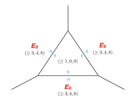
Figure 2: The initally blown up $E_{6}$–$E_{6}$–$E_{6}$ Yukawa point.

5.2.2 $E_{6}\times E_{6}\times E_{6}$

Turning to the case in which each divisor has type $E_{6}$, we can represent this by the equation

$$y^{2}=x^{3}+(uvw)^{4}$$ (5.17)

with $\Delta=27(uvw)^{8}$. (In this case, $f$ is not relevant for the computations and we may as well set it equal to $0$.) Along curves of intersection such as $u=v=0$, we find $E_{6}$–$E_{6}$ conformal matter, and those non-compact curves could be blown up. Rather than doing so, however, we examine the Yukawa point.

The multiplicities of $(f,g,\Delta)$ at the origin are $(\geq 9,12,24)$ which means that the origin may be blown up. The residual vanishing of $(f_{0},g_{0},\Delta_{0})$ (after reducing the orders of vanishing by $(8,12,24)$) are $(\geq 1,0,0)$. Thus, we have Kodaira type $I_{0}$ (nonsingular elliptic fibers) over the exceptional divisor $E$. There are three new Yukawa points introduced by this blowup, but they each have multiplicities $(\geq 6,8,16)$ which does not allow a blowup. In addition, no new curves of conformal matter were introduced by this blowup, but of course we still have the original three noncompact conformal matter curves. The exceptional divisor is $\mathbb{P}^{2}$ and it meets the other exceptional divisors in lines (which have self-intersection $1$). These same lines are exceptional curves of self-intersection $-1$ within the blown up divisor. All of this is illustrated in figure 2, in which we give both the gauge or flavor group and the orders of vanishing of $(f,g,\Delta)$ for each divisor. (When the divisor is unlabeled, there is no gauge symmetry or flavor symmetry associated to that divisor.)

We next blow up the non-compact conformal matter curves (see figure 3). The pattern of the blowups is determined by the $E_{6}$–$E_{6}$ collision (known as the $IV^{*}$–$IV^{*}$ collision in Kodaira notation) whose sequence of blowups was determined long ago [12, 70].

Note that when blowing up a non-compact conformal matter curve $\Gamma$ we automatically blowup the point of intersection of $\Gamma$ with any divisor $D$, creating an exceptional curve $C$ on the blow up of $D$. The self-intersection of $C$ is $-1$ on the blown up divisor $\widetilde{D}$ and is $0$ on the non-compact exceptional divisor. Moreover, any curve on $D$ which passes through the point being blown up will have its self-intersections lowered on $\widetilde{D}$. All of these properties are visible in figure 3, which shows the results of an iterated sequence of blowups.

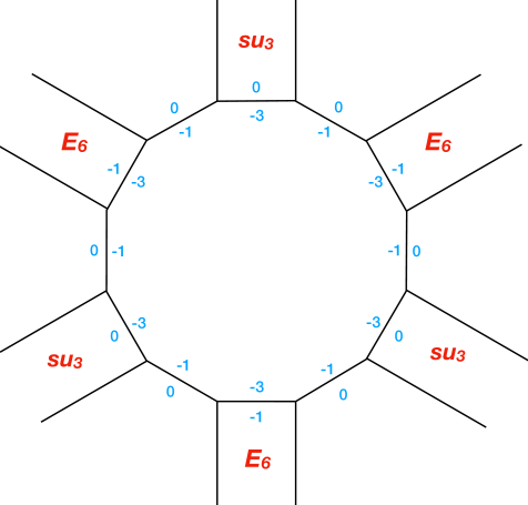
Figure 3: The fully blown up $E_{6}$–$E_{6}$–$E_{6}$ Yukawa point.

5.2.3 $E_{7}\times E_{7}\times E_{7}$

The next case to consider is the one in which each divisor has type $E_{7}$. We can represent this by the equation

$$y^{2}=x^{3}+(uvw)^{3}x$$ (5.18)

with $\Delta=4(uvw)^{9}$. (In this case, it is $g$ which is not relevant for the computations and which we set to $0$.) Along curves of intersection such as $u=v=0$, we find $E_{7}$–$E_{7}$ conformal matter. We first examine the Yukawa point without blowing up the conformal matter curves.

The multiplicities of $(f,g,\Delta)$ at the origin are $(9,\geq 15,27)$ which means that the origin should be blown up. The residual vanishing of $(f_{0},g_{0},\Delta_{0})$ (after reducing the orders of vanishing by $(8,12,24)$) are $(1,\geq 3,3)$, which is Kodaira type $III$ with gauge group $SU(2)$ over the exceptional divisor $E$. There are three new Yukawa points introduced by this blowup, but they each have multiplicities $(7,\geq 13,21)$ which does not allow a blowup. There are also three new compact conformal matter curves introduced by this blowup, each having $E_{7}$–$SU(2)$ conformal matter. These could also be blown up if desired, but we shall postpone doing so. The illustration of this initial blowup is in figure 4, in which we again give both the gauge group and the orders of vanishing of $(f,g,\Delta)$ for each divisor.

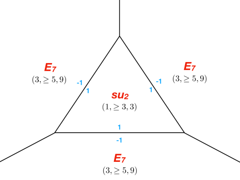
Figure 4: The initially blown up $E_{7}$–$E_{7}$–$E_{7}$ Yukawa point.

We now blow up the non-compact conformal matter curves, this time relying on the known sequence of blowups for the $E_{7}$–$E_{7}$ collision (also known as the $III^{*}$–$III^{*}$ collision). At the end of this process, there are still three compact curves supporting conformal matter of $E_{7}$–$SU(2)$ type (also known as $III^{*}$–$III$ type). Blowing up those compact curves one time each completes the resolution, illustrated in figure 5.

In general, when we blow up a compact curve $\Gamma$ which is the intersection of two divisors in which the self-intersections are $-a$ and $-b$, the normal bundle of the curve in the threefold is $\mathcal{O}(-a)\oplus\mathcal{O}(-b)$. Blowing up the curve creates the Hirzebruch surface $\mathbb{F}_{a-b}$. That surface is ruled with curves of self-intersection $0$ (which may appear as exceptional curves of self-intersection $-1$ on other divisors). Moreover, there are two disjoint sections, with self-intersection $a-b$ and $b-a$.

In particular, there are two new compact curves: one with normal bundle $\mathcal{O}(-a)\oplus\mathcal{O}(a-b)$ and the other with normal bundle $\mathcal{O}(b-a)\oplus\mathcal{O}(-b)$. In the present example, the last three blowups are on curves with normal bundle $\mathcal{O}(-1)\oplus\mathcal{O}(-5)$. Blowing each of them up creates a Hirzebruch surface $\mathbb{F}_{4}$ and two curves on it: one with normal bundle $\mathcal{O}(-1)\oplus\mathcal{O}(-4)$ and the other with normal bundle $\mathcal{O}(4)\oplus\mathcal{O}(-5)$.

All of these features are visible in figure 5.

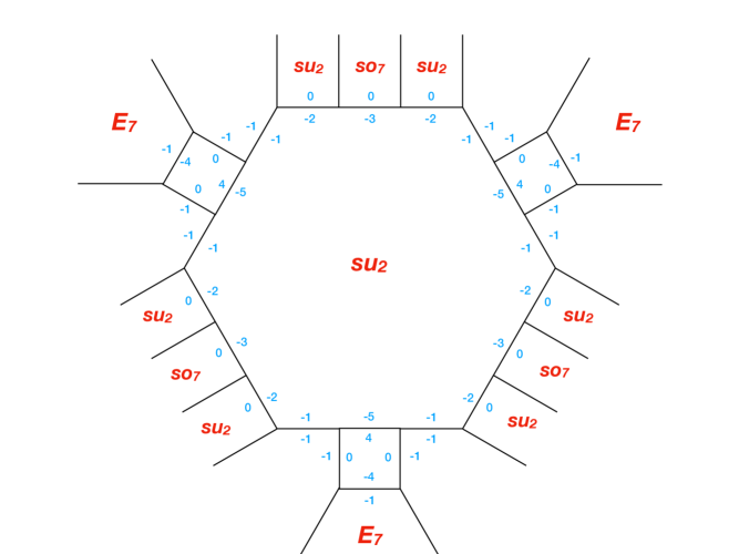
Figure 5: The fully blown up $E_{7}$–$E_{7}$–$E_{7}$ Yukawa point.

5.2.4 $E_{8}\times E_{8}\times E_{8}$

As our last example with constant $J$-invariant, we let each divisor have type $E_{8}$ which we can represent by the equation

$$y^{2}=x^{3}+(uvw)^{5}$$ (5.19)

with $\Delta=27(uvw)^{10}$. (Once again, $f$ is not relevant for the computations and which we set to $0$.) Along curves of intersection of pairs of divisors, we find $E_{8}$–$E_{8}$ conformal matter. We will first examine the Yukawa point without blowing up the conformal matter curves.

The multiplicities of $(f,g,\Delta)$ at the origin are $(\geq 12,15,30)$ which means that the origin should be blown up. The residual vanishing of $(f_{0},g_{0},\Delta_{0})$ (after reducing the orders of vanishing by $(8,12,24)$) are $(\geq 4,3,6)$, which is Kodaira type $I_{0}^{*}$ with gauge group $G_{2}$ over the exceptional divisor $E$. There are three new Yukawa points introduced by this blowup. Each has multiplicities $(\geq 12,13,26)$ so that they can be blown up. Blowing them up will generate three more exceptional divisors $E_{1}$, $E_{2}$, $E_{3}$, each of which has residual multiplicities $(\geq 4,1,2)$ and hence Kodaira type $II$. This is the Kodaira type which does not have any gauge symmetry, and yet for which the elliptic fibers in the total space are singular (with cusps). An intersection curve between a divisor of Kodaira type $II$ and an $E_{8}$ divisor has conformal matter with global symmetry $E_{8}$ and that must be considered in this situation. For this reason, we are careful to label the type $II$ divisors even though there is no gauge or flavor symmetry associated to them. The configuration of divisors and gauge groups after the initial blowups of Yukawa points is illustrated in figure 6.

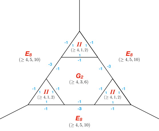
Figure 6: The initially blown up $E_{8}$–$E_{8}$–$E_{8}$ Yukawa point.

After the four blowups at points, we are left with the original three noncompact $E_{8}$–$E_{8}$ (or $II^{*}$–$II^{*}$) conformal matter curves, supplemented by three compact $G_{2}$–$E_{8}$ (or $I_{0}^{*}$–$II^{*}$) conformal matter curves, and six $II$–$E_{8}$ (or $II$–$II^{*}$) conformal matter curves.

We blow the conformal matter curves up in two steps. First, we use the known sequence of blowups for the $G_{2}$–$E_{8}$ collision to resolve the conformal matter there. The known sequence of blowups includes information of about gauge algebras, and the rules articulated above allow the determination of the self-intersection of each compact curve in the diagram. The results are illustrated in figure 7.

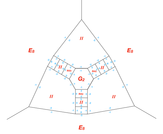
Figure 7: The partially blown up $E_{8}$–$E_{8}$–$E_{8}$ Yukawa point.

In the final step, just as in the $E_{7}$–$E_{7}$–$E_{7}$ case we blow up the non-compact conformal matter curves using the known blowup sequence and flavor groups for the $II^{*}$–$II^{*}$ collision. Finally, we blow up the six remaining $II$–$II^{*}$ collisions, obtaining a Hirzebruch $\mathbb{F}_{6}$ in each case. The result is illustrated in figure 8.

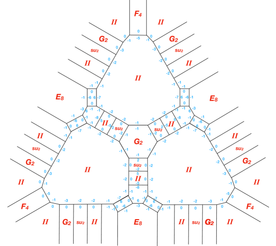
Figure 8: The completely blown up $E_{8}$–$E_{8}$–$E_{8}$ Yukawa point.

5.2.5 Mixed G’s with Non-Constant J-function

As a final example, we treat a case with non-constant $J$-function. The computations are dependent on both $f$ and $g$, and in fact we can get variable answers depending on apparently subtle details of the equation. We allow the three divisors to have gauge symmetry $E_{6}$, $E_{7}$ and $E_{8}$ which we can realize in a variety of ways with the Weierstrass equation

$$y^{2}=x^{3}+u^{3+k}v^{3}w^{4+m}x+u^{4}v^{5+\ell}w^{5}$$ (5.20)

for various choices of nonnegative integers $k\geq 0$, $\ell\geq 0$, and $m\geq 0$. The discriminant takes the form

$$4u^{9+3k}v^{9}w^{12+3m}+27u^{8}v^{10+2\ell}w^{10}=u^{8}v^{9}w^{10}(4u^{3k+1}w^{3m+2}+27v^{2\ell+1})$$ (5.21)

and has multiplicity at the origin $27+\operatorname{min}(3k+3m+3,2\ell+1)$. In particular, the multiplicity is $28$ if $k=\ell=m=0$. The multiplicities of $f$ and $g$ at the origin are $(10+k+m,14+\ell)$.

The origin can be blown up, leaving residual orders of vanishing

$$(2+k+m,2+\ell,4+\operatorname{min}(3k+3m+2,2\ell));$$ (5.22)

the minimum value is $(2,2,4)$. As can be seen, the minimum value has Kodaira type $IV$, but other values are possible. For example, $\ell=1$ implies Kodaira type $I_{0}^{*}$. As another example, if $\ell=2$ and $k+m=1$ we get Kodaira type $IV^{*}$ (and gauge group $E_{6}$).

Let us analyze the minimal case $k=\ell=m=0$. The Kodaira type after the first blowup is $IV$ with gauge group $SU(3)$. There are three new Yukawa points created after the first blowup, and again, assessing the multiplicity of $\Delta$ is tricky. If $\{t=0\}$ is the new exceptional divisor, then the Weierstrass equation after the first blowup can be written

$$y^{2}=x^{3}+t^{2}u^{3}v^{3}w^{4}x+t^{2}u^{4}v^{5}w^{5}$$ (5.23)

with discriminant $t^{4}u^{8}v^{9}w^{10}(4t^{2}uw^{2}+27v)$. It follows that the discriminant has multiplicity higher than naively expected if $t=u=v=0$ or $t=v=w=0$. Thus, the multiplicities at the three new Yukawa points are $(8,11,22)$, $(9,11,22)$, and $(9,12,24)$. Only the last one can be blown up, and it gives an exceptional divisor of Kodaira type $I_{0}$ with a nonsingular elliptic fibration over it. This is illustrated in figure 9.

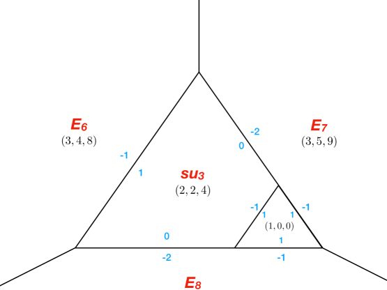
Figure 9: The blowup of the minimal $E_{6}-E_{7}-E_{8}$ Yukawa point.

We omit the description of the complete blowup in this case.

5.3 Quiver Networks in F-theory

Clearly, there are many ways we can piece together the codimension one, two and three singularities of the threefold base to engineer 4D quantum field theories. Indeed, in addition to these geometric ingredients there will also be fluxes from 7-branes which allow us to induce a “chiral spectrum” on each conformal matter curve.

From the perspective of F-theory, a particularly simple class of examples involve taking the base to be a non-compact toric Calabi-Yau threefold. In this case, the analysis of the previous sections illustrates that for any associated $(p,q)$ web diagram describing a toric Calabi-Yau threefold, we can decorate each face (be it compact or non-compact) by wrapping a 7-brane over it. This clearly produces a quiver-like structure, in which the bifundamentals are 4D conformal matter compactified on compact legs of the geometry, and with Yukawa couplings between the 4D conformal matter. The analysis of resolutions of singularities presented in the previous subsection illustrates that this also leads to a well-defined elliptically fibered Calabi-Yau fourfold, albeit one with many canonical singularities. An interesting feature of this classical geometry is the presence of a large flavor symmetry group. By inspection, there is a complex structure deformation which takes the “pinched” complex curves meeting at conformal Yukawas to the case of a single smooth curve of 4D conformal matter compactified on a high genus curve (see for example figure 10, for a single $dP_{3}$ intersecting six non-compact surfaces all with the same group $G$.)

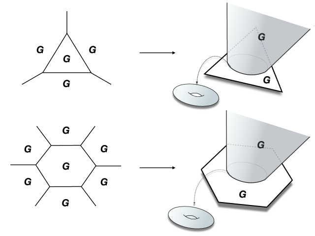
Figure 10: On the left mutually meeting non-compact surfaces with group $G$ and all meeting at a compact $\mathbb{P}^{2}$ (toric diagram: triangle) on top, or $dP_{3}$ (toric diagram, hexagon) on the bottom with gauge group $G$ on $\mathbb{P}^{1}$ curves. On the right the smoothing where a recombined non-compact surfaces intersects the $dP_{3}$ or $\mathbb{P}^{2}$ on a $T^{2}$.

As an illustrative example, consider a 7-brane with gauge group $E_{8}$ wrapped on a compact $\mathbb{P}^{2}$ which intersects a non-compact $E_{8}$ flavor 7-brane. The local Weierstrass model for this geometry has already been given on line (5.8) which we reproduce for the convenience of the reader:

$$y^{2}=x^{3}+v^{5}(\widetilde{g}_{\Sigma})^{5}\text{,}$$ (5.24)

In this equation, $\widetilde{g}_{\Sigma}$ is a section of the bundle $\mathcal{O}(3H)$ with $H$ the hyperplane class divisor, namely a degree three homogeneous polynomial on $\mathbb{P}^{2}$ with vanishing locus an elliptic curve. We can further specialize the form of this polynomial by factoring the cubic into three linear terms:

$$\widetilde{g}_{\Sigma}=\underset{i=1}{\overset{3}{{\displaystyle\prod}}}\widetilde{g}_{i}.$$ (5.25)

Plugging back in to our minimal Weierstrass model, the geometry now includes the appearance of Yukawas between conformal matter sectors:

$$y^{2}=x^{3}+v^{5}(\widetilde{g}_{1}\widetilde{g}_{2}\widetilde{g}_{3})^{5}\text{,}$$ (5.26)

so the classical geometry now has three $E_{8}$ flavor symmetries! Additionally, there are now codimension three singularities in the threefold base along which three $E_{8}$ factors meet.

Similar considerations hold for 7-branes wrapped on other compact surfaces. As a more involved example, we can consider a toric threefold base tiled by a honeycomb lattice as in figure 11. Each hexagon in this lattice describes a local del Pezzo three geometry $dP_{3}$, namely $\mathbb{P}^{2}$ blown up at three points in general position. Observe that in the case of a single hexagon, the local geometry is again given by the same sort of Weierstrass models described previously. For example, in the collision of two $E_{8}$ 7-branes, we again have a complex equation as in line (5.24), but where now, $\widetilde{g}_{\Sigma}$ is a section of $\mathcal{O}(-K_{\mathcal{S}})$, namely the vanishing locus is the anti-canonical divisor. Recall that the ring of divisors for the surface $dP_{3}$ has generators $H$, the hyperplane class, and $E_{i}$ three exceptional divisors. In terms of these generators, we have:

$$\mathcal{O}(-K_{\mathcal{S}})=\mathcal{O(}3H-E_{1}-E_{2}-E_{3}\mathcal{)}\text{.}$$ (5.27)

By suitable tuning, we can further factorize $\widetilde{g}_{\Sigma}$ so that the elliptic curve degenerates into a necklace of six lines:

$$\widetilde{g}_{\Sigma}=\widetilde{g}_{1}\widetilde{g}_{12}\widetilde{g}_{2}\widetilde{g}_{23}\widetilde{g}_{3}\widetilde{g}_{31},$$ (5.28)

where these polynomials are sections of the following bundles:

$$\widetilde{g}_{i}\in\mathcal{O(}E_{i}\mathcal{)}\text{ \ \ and \ \ }\widetilde{g}_{ij}\in\mathcal{O(}H-E_{i}-E_{j}\mathcal{)}\text{.}$$ (5.29)

Doing so, we see that the entire honeycomb lattice can be filled with gauge groups of $E_{8}$ type with non-compact flavor branes on the outside of the picture. Similar considerations clearly hold for other choices of gauge groups, and lead to a vast array of quantum field theories.

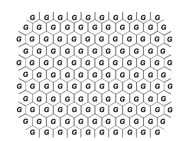
Figure 11: Toric diagram for a threefold base $\mathcal{B}$. Here, each compact face of the honeycomb represents a $dP_{3}$ surface. By suitable tuning of the elliptic fiber, we can wrap 7-branes with gauge group $G$ over each face of the geometry.

Note that in the construction of these networks of quiver gauge theories, we can also see the presence of pinched off curves which meet at trivalent junctions. Applying a smoothing deformation, we see that generically, these curves can fatten up into a high genus curve, and applying a further smoothing deformation eliminates all the compact gauge group factors.

It is natural to ask whether this tuning operation has a counterpart in the field theory. To properly address this issue, we will need to study quantum corrections to the geometry. In particular, we shall present evidence that quantum corrections smooth out such tunings, lifting such enhancements points from the quantum moduli space.

5.4 Quantum Corrected Geometry

So far, we have focussed on the classical geometry specified by our F-theory background. We have also seen that generically, the quiver gauge theories constructed have compact complex surfaces. This includes the 7-branes wrapped over the gauge theory divisors of the F-theory model, but also includes additional collapsing surfaces associated with the codimension three singularities present in the base.

Now, it is well known from the analysis of [106] that the presence of such surfaces can generate quantum corrections which generically mix the complex structure and Kähler moduli of an F-theory background. In F-theory terms, this comes about from Euclidean D3-branes wrapped over compact surfaces of the model. In the M-theory background defined by reduction on a circle, these instanton corrections are captured by Euclidean M5-branes wrapped on divisors of the Calabi-Yau fourfold.

In either the F-theory description or its dimensional reduction in M-theory, the assessing the presence (or absence) of such instanton corrections amounts to a multi-step process. First, we must determine the spectrum of light states stretched between our Euclidean brane and the other branes present in the background (now treated as fixed objects). Next, integrating over the zero mode moduli space, and also possible flux sectors from the Euclidean brane then leads to instanton corrections to the F- and D-terms of the 4D quantum field theory.

The first aspect of determining whether instanton corrections can be generated should be clear. In the F-theory models considered, we clearly have compact surfaces which can be wrapped, so we ought to generically expect the presence of instanton corrections. Note that even in the case of the $SO(n)^{3}$ codimension three singularities, we should expect instanton corrections. The reason is that even though the resolved geometry contains no compact complex surfaces, it contains compact curves in an F-theory background with constant axio-dilaton. In such configurations, Euclidean D1- and F1-strings can wrap the complex curves, again generating a quantum deformation of the classical moduli space.

The second aspect, where we actually attempt to extract the zero mode spectrum for states stretched between the Euclidean brane and the background branes of the geometry is more challenging in general due to the presence of exceptional 7-branes. Simliar systems with D3-branes in the presence of exceptional 7-branes often lead to strongly interacting SCFTs [107, 108]. In our case, these exceptional 7-branes can either share four common directions with the Euclidean D3-brane, or intersect along a complex curve.

Though it would clearly be interesting to directly calculate the form of these superpotential deformations from this perspective, our primary aim in this work will be to determine when to expect such corrections to the classical geometry. So, we shall instead piece together our bottom up and top down considerations to analyze the quantum corrected moduli space.

The first situation where we can track the effects of an instanton correction comes from the SQCD-like theory with generalized quiver:

$$(G)\overset{CM}{-}[G].$$ (5.30)

From our field theory considerations, we expect an instanton correction to contribute which deforms the moduli space of vacua, namely the origin of the mesonic branch of moduli space will be lifted. By inspection of the F-theory geometry where we have a 7-brane wrapped on a compact surface, we can see that a Euclidean D3-brane could indeed wrap this surface. In the F-theory construction, however, the gauge coupling is promoted to a dynamical field, so in contrast to equation (3.33), we now get the relation (see also [93]):

$$\text{Cas}_{\text{max}}(M_{R})-(\text{Baryons})=\left(\Lambda_{UV}\times\exp(2\pi iT)\right)^{b_{G}}\text{,}$$ (5.31)

where $T$ is the complexified volume modulus associated with the compact complex surface in the geometry. From the perspective of the effective field theory, we can introduce a chiral superfield:

$$X=\Lambda_{UV}\times\exp(2\pi iT).$$ (5.32)

The non-trivial element in this identification is that the origin of the $X$ moduli space corresponds to decompactifying the surface $\mathcal{S}$.

This sort of correction term mixes the complex structure moduli with the Kähler moduli. Additionally, it triggers a brane recombination. For example, in the case where $G=E_{8}$, the deformation is of the form:

$$y^{2}=x^{3}+v^{5}(\widetilde{g}_{\Sigma})^{5}\rightarrow y^{2}=x^{3}+\left(v\widetilde{g}_{\Sigma}-r\right)^{5},$$ (5.33)

with $r$ a recombination mode coming from the vevs of the meson fields. It would be interesting to perform a direct calculation of this effect in string theory, perhaps along the lines of references [106, 109].

More generally, we can see that complex structure deformations of the F-theory model translate to “mesonic deformations” of the field theory. T-brane deformations which retain the form of the Weierstrass model are thus natural candidates for “baryonic deformations.”

Consider next the F-theory model defined by a triple intersection of three $G$-type 7-branes. For ease of exposition, we focus on the special case where $G=E_{8}$, which as we have already remarked, is described by a minimal Weierstrass model of the form:

$$y^{2}=x^{3}+(uvw)^{5}.$$ (5.34)

The resolution of this codimension three singularity introduces compact Kähler surfaces, so there is the possibility of an instanton correction.

In this case, we see that the classical geometry consists of three semi-infinite tubes of 6D conformal matter which are being joined together at a singular point of the geometry. It identifies the flavor symmetries of each tube so that we have a $G_{\text{classical}}=E_{8}\times E_{8}\times E_{8}$ flavor symmetry classically.

Let us compare this with compactifications of class $\mathcal{S}_{\Gamma}$ theories. In the present case, the F-theory geometry suggests that we look at a theory on a thrice punctured sphere which retains a $G_{\text{classical}}$ flavor symmetry. By inspection of the family of metrics for the thrice punctured sphere, however, we see that there is no degeneration in the family of metrics which will take us from this smooth geometry to that in which three tubes degenerate. Moreover, there does not appear to be a point in the moduli space of theories in which an enhancement to $G_{\text{classical}}$ occurs, even taking into account data near the punctures. Indeed, in the present case the F-theory model suggests that all boundary conditions at these marked points are trivial, so the best we could hope for from the M-theory construction is an $E_{8}\times E_{8}$ flavor symmetry (though even this is typically broken to a smaller flavor symmetry).

Another awkward feature of this construction from the perspective of class $\mathcal{S}_{\Gamma}$ theories is that the volume of the tubes becomes larger as we proceed away from the trivalent junction. This is precisely the opposite situation to what one expects to encounter for a punctured Riemann surface.

This strongly suggests that the classical F-theory picture cannot be realized in the class $\mathcal{S}_{\Gamma}$ construction. We thus have two options: Either the F-theory picture receives no quantum corrections – in spite of the presence of collapsing divisors in the base –, or instead the F-theory geometry receives quantum corrections which smooth out some of these singularities. The latter scenario seems far more plausible, and presents a self-consistent picture. See figure 12 for a depiction of this smoothing process.

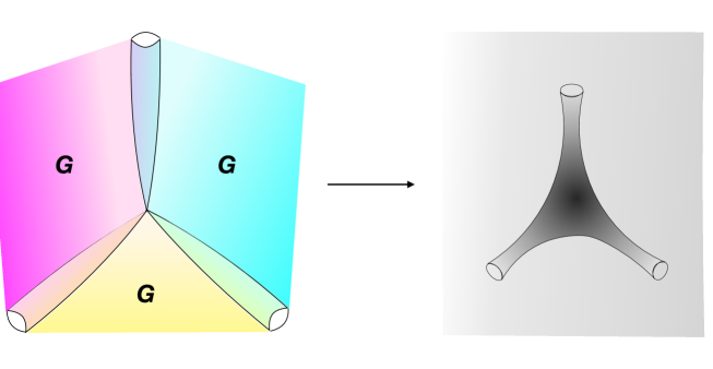
Figure 12: On the left three non-compact surfaces with group $G$ mutually meeting on cigar geometries, which intersect at a point. On the right the smoothing of the configuration to a single surface (grey) where only a subgroup $H\subset G$ may survive.

Hence, we expect a smoothing deformation to rejoin the three complex lines $u=0$, $v=0$, $w=0$ into a single cubic polynomial in the variables $(u,v,w)$ which need not factorize. Denoting this as $\widetilde{g}_{3}(u_{i})$, we see that the presence of such codimension three singularities will be accompanied by a smoothing deformation:

$$y^{2}=x^{3}+(uvw)^{5}\rightarrow y^{2}=x^{3}+(\widetilde{g}_{3}(u,v,w))^{5},$$ (5.35)

so that only a single $E_{8}$ survives.

More generally, we expect that Yukawas for 4D conformal matter lead to smoothings from factorized curves to more generic curves.

These two sorts of instanton corrections can also appear simultaneously in a given F-theory background. As an example of this sort, consider again the model specified by line (5.24), with Weierstrass model:

$$y^{2}=x^{3}+v^{5}(\widetilde{g}_{1}\widetilde{g}_{2}\widetilde{g}_{3})^{5}\text{.}$$ (5.36)

By inspection, we see three codimension three enhancement points at the torus fixed points of the $\mathbb{P}^{2}$. We thus expect a quantum deformation which eliminates this tuned factorization, leading to smoothings of $v$ and a pair $g_{i}$ and $g_{j}$. If, however, we assume that this smoothing leaves intact the presence of the $E_{8}$ gauge group on $v=0$, then the form of this smoothing is further constrained to take the form:

$$y^{2}=x^{3}+v^{5}(\widetilde{g}_{1}\widetilde{g}_{2}\widetilde{g}_{3})^{5}\rightarrow y^{2}=x^{3}+v^{5}(\widetilde{g}_{3H})^{5}.$$ (5.37)

But this is the model $(E_{8})\overset{CM}{-}[E_{8}]$, which also confines, so the net result of the deformations is:

$$y^{2}=x^{3}+v^{5}(\widetilde{g}_{1}\widetilde{g}_{2}\widetilde{g}_{3})^{5}\rightarrow y^{2}=x^{3}+v^{5}(\widetilde{g}_{3H})^{5}\rightarrow y^{2}=x^{3}+(v\widetilde{g}_{3H}-r)^{5}$$ (5.38)

in the obvious notation. Namely, the mesonic fields pick up a non-zero vev and break to the diagonal $E_{8}$ which is a flavor symmetry.

Similar considerations clearly apply in the network defined by the honeycomb lattice of figure 11. Even though the classical geometry contains a large flavor symmetry group, quantum deformations to the moduli space lead in the infrared to a confining phase.

5.4.1 Conformal Fixed Points

In some cases, instantons do not produce such strong deformations of the classical moduli space. An example of this type is the intersection of two $E_{6}$ 7-branes along a genus three curve. We know from our field theory analysis that weakly gauging one of the $E_{6}$ factors leads to a conformal fixed point at the top of the conformal window for $E_{6}$ gauge theory. This involves “genus three” conformal matter. Based on the analysis of Appendix B, we also see that once we incorporate fluxes from the 7-branes, we can again engineer conformal fixed points.

It is also possible to engineer examples of conformal fixed points without resorting to the presence of higher genus or 7-brane fluxes. To give an example of this type, we now engineer the 4D model:

$$[E_{8}]\overset{CM}{-}\overset{[E_{8}]}{\overset{|}{(E_{8})}}\overset{CM}{-}[E_{8}].$$ (5.39)

We take our gauge theory surface to be a $dP_{9}$. This surface can be viewed as a $\mathbb{P}^{2}$ blown up at nine points in general position, but can also be viewed as an elliptically fibered surface over a base $\mathbb{P}^{1}$. In the latter description, we can mark three points, each of which is associated with a $T^{2}$. The local Weierstrass model is then:

$$y^{2}=x^{3}+v^{5}(\widetilde{g}_{1}\widetilde{g}_{2}\widetilde{g}_{3})^{5},$$ (5.40)

where the divisor class of each $\widetilde{g}_{i}$ is $3H-E_{1}-...-E_{9}$, with $E_{1},...,E_{9}$ the nine exceptional divisors of the surface. The three matter curves do not intersect, so there are no conformal Yukawas present in the model. Note that in this case, the local threefold cannot be a Calabi-Yau, since as we have already remarked, that would have corresponded to having a single genus one 4D conformal matter sector. Instead, we learn that since the product $\widetilde{g}_{1}\widetilde{g}_{2}\widetilde{g}_{3}$ is a section of the bundle $\mathcal{O}_{\mathcal{S}}\left(-3K_{\mathcal{S}}\right)$, we require the divisor relation:

$$\frac{-6K_{\mathcal{S}}+\mathcal{S}\cdot\mathcal{S}}{5}=-3K_{\mathcal{S}}.$$ (5.41)

So, the self-intersection of $\mathcal{S}$ in the threefold base is fixed to be:

$$\mathcal{S}\cdot\mathcal{S}=-9K_{\mathcal{S}}.$$ (5.42)

In other words, the threefold base is locally given by the total space $\mathcal{O}(-9K_{\mathcal{S}})\rightarrow\mathcal{S}$. Even though the gauge theory surface is not a contractible cycle in the threefold base, the 4D gauge theory appears to make sense in its own right.

6 Conclusions

Compactifications of 6D conformal matter on curves lead to novel building blocks in the construction and study of strongly coupled quantum field theories in four dimensions. The main idea in our construction is that by weakly gauging the flavor symmetries of such theories by 4D $\mathcal{N}=1$ vector multiplets, we can obtain a broad class of quiver-like gauge theories in which the link fields are themselves strongly coupled sectors. We have presented evidence from a bottom up perspective that much as in ordinary SQCD with classical gauge groups, there is a notion of a conformal window with 4D conformal matter, and that the analog of SQCD with gauge group $SU(N_{c})$ and $N_{f}=N_{c}$ flavors leads to a confining gauge theory. We have also presented a top down construction of this and related quantum field theories using F-theory on elliptically fibered Calabi-Yau fourfolds in the presence of canonical singularities. An additional ingredient suggested by the F-theory models is the presence of Yukawa couplings between 4D conformal matter, which in geometric terms is associated with codimension three points in the base where the multiplicities of the Weierstrass model coefficients $f$, $g$ and the discriminant $\Delta$ are at least $(8,12,24)$, respectively. Combining our bottom up and top down analyses, we have also argued that the presence of collapsing four-cycles in these geometries generically indicates the presence of Euclidean D3-brane instanton corrections which mix the Kähler and complex structure moduli. Moreover, they can often smooth out some singularities present in the classical geometries. This suggests a wide variety of applications within both field theory and F-theory. In the rest of this section we indicate some potential avenues for future investigation.

We have pieced together evidence for instanton corrections to the classical moduli space, based mainly on consistency with both bottom up and top down considerations. Given that we have the explicit F-theory geometry for these 4D theories, it should in principle be possible to carefully track the worldvolume theory of Euclidean D3-branes to calculate such superpotential corrections. Though the worldvolume theory of these D3-branes may have some non-Lagrangian building blocks, one of the guiding philosophies of this work has been that such effects can often still be analyzed, so it would seem worthwhile to see whether a direct stringy calculation could indeed be performed, perhaps along the lines of references [110, 111, 112].

One of the most intriguing features of SQCD with classical gauge groups and matter content is the notion of Seiberg duality. It is tempting to extend such considerations to the case of exceptional gauge groups with 4D conformal matter. To carry this out geometrically, we would need to understand the structure of flop transitions in the models just engineered. Alternatively, we could attempt to make an educated guess as to the nature of Seiberg duals for gauge theories with 4D conformal matter. This would provide additional insight into the structure of strongly coupled 4D field theories.

Much as in other cases, engineering these 4D field theories turns out to be simplest in cases where we can leverage the full power of holomorphic geometry. This in particular is the reason we have chosen F-theory to analyze the string theory lift of the resulting 4D quantum field theories. Even so, it is tempting to directly engineer these systems using M-theory on a singular manifold with $G_{2}$ metric holonomy. In this description, weakly gauging a flavor symmetry amounts to introducing compact three-cycles (presumably calibrated with respect to the associative three-form). There are in principle two ways that one could introduce 4D conformal matter in this setting. One way is to simply wrap M5-branes on two-cycles of the geometry. Another way would be to consider specialized intersections of three-cycles along Riemann surfaces. Turning the discussion around, the successful realization of these structures in F-theory strongly suggests there is also an M-theory avatar for constructing such geometries. This would likely provide further insight into the construction of $G_{2}$ manifolds.

Another natural direction to consider is the extension of these results to the construction of 2D quantum field theories. References [46, 113, 114, 115] have initiated a general program for engineering 2D quantum field theories via compactifications of F-theory on elliptically fibered Calabi-Yau fivefolds. Continuing in the same vein as in the 4D case, we can clearly see a similar quiver-like structure with exceptional gauge groups and 2D conformal matter will be present in this lower dimensional case. Note that in this case it is also natural to consider quartic intersections of 7-branes when the multiplicities of the Weierstrass model coefficients $f$, $g$ and the discriminant $\Delta$ are at least $(12,18,36)$, respectively. It would be quite interesting to study the resulting field theories engineered from this starting point.

Appendix A $(4,6,12)$ and all that

As has been discussed since the earliest days of F-theory [7, 116], in a Weierstrass model

$$y^{2}=x^{3}+fx+g$$ (A.1)

over a base $\mathcal{B}$, if the orders of vanishing of $f$, $g$, and $\Delta:=4f^{3}+27g^{2}$ exceed $(4,6,12)$ along some divisor, then the singularities are bad enough to destroy the Calabi–Yau property of the total space. For example, in the simplest case

$$y^{2}=x^{3}+f_{0}\,t^{4}x+g_{0}\,t^{6}$$ (A.2)

(with $f_{0}$ and $g_{0}$ constant), the corresponding surface singularity can be resolved by a weighted blowup [117] with the weights of $t$, $x$, and $y$ being $1$, $2$, and $3$, respectively. The exceptional divisor $E$ of the weighted blowup is an elliptic curve of self-intersection $-1$ of weighted degree $6$ in $\mathbb{P}^{1,2,3}$ (see Example 2.5 in [118] for details). The original fiber has its cusp singularity resolved, and becomes a nonsingular rational curve $C$ of self-intersection $-1$ meeting $E$ transversally. Moreover, the holomorphic $2$-form on the Weierstrass model acquires a pole along $E$ when we blow up and the blowup no longer has trivial canonical bundle. By the Hayakawa-Wang criterion [119, 120], in type IIA or M-theory on the corresponding Calabi–Yau moduli space, such points are at infinite distance from the interior of moduli (and so they should be in F-theory as well).

The curve $C$ can be blown down to a smooth point, and doing so increases the self-intersection of $E$ to $0$; $E$ is now a fiber of an elliptic fibration. But the total space no longer has trivial canonical bundle. The easiest way to see this is to divide (A.2) by $t^{6}$ and rewrite as

$$(y/t^{3})^{2}=(x/t^{2})^{3}+f_{0}\,(x/t^{2})+g_{0},$$ (A.3)

or, introducing new variables $X=x/t^{2}$, $Y=y/t^{3}$,

$$Y^{2}=X^{3}+f_{0}\,X+g_{0}.$$ (A.4)

If $x$, $y$, $f$, and $g$ were sections of $\mathcal{O}(-2K_{B})$, $\mathcal{O}(-3K_{B})$, $\mathcal{O}(-4K_{B})$, and $\mathcal{O}(-6K_{B})$, respectively (as needed for a Calabi–Yau total space), then $X$, $Y$, $f_{0}$, and $g_{0}$ are sections of $\mathcal{O}(-2K_{B}-2D)$, $\mathcal{O}(-3K_{B}-3D)$, $\mathcal{O}(-4K_{B}-4D)$, and $\mathcal{O}(-6K_{B}-6D)$, respectively, where $D$ is the divisor $\{t=0\}$. Thus, the “wrong” line bundle $\mathcal{O}(K_{B}+D)$ is being used for the Weierstrass model, and the canonical bundle of the total space is not trivial.

The argument we have just given applies in any dimension, with $\{t=0\}$ a local equation for a divisor $D$ along which $f$ vanishes to order at least $4$ and $g$ vanishes to order at least $6$. More generally, if we had started with a Weierstress model which was based on a line bundle $\mathcal{L}$ (not necessarily $\mathcal{O}(K_{\mathcal{B}})$) then this construction changes it to the bundle $\mathcal{L}\otimes\mathcal{O}(D)$.

Suppose now that we replace the divisor $D$ by a locus $\Gamma$ of higher codimension. (For example, $\Gamma$ could be a point when $\mathcal{B}$ is a surface, $\Gamma$ could be a point or a curve when $\mathcal{B}$ is a threefold, and so on.) In this case, if $f$ and $g$ have sufficiently large multiplicity along $\Gamma$, it signals the possibility of blowing up the base $\mathcal{B}$ without disturbing the Calabi–Yau condition. We now explain how this works.

Let $k\geq 2$ denote the codimension of $\Gamma$ and suppose that $\Gamma$ is locally defined by the vanishing of $k$ functions $\{x_{1}=x_{2}=\cdots=x_{k}=0\}$ which are part of a local coordinate system (i.e., the other coordinates are $x_{k+1}$, …, $x_{n}$ where $n$ is the dimension of $\mathcal{B}$). A sample coordinate chart on the blowup has coordinates $u_{j}=x_{j}/x_{k}$ for $j=1,\dots,k-1$ and then $x_{k}$, $x_{k+1}$, …, $x_{n}$ with $\{x_{k}=0\}$ defining the exceptional divisor $E$ of the blowup. Then we have

$$\pi^{*}(f(x_{1},\dots,x_{n})\,dx_{1}\wedge dx_{2}\wedge\cdots\wedge dx_{k-1}\wedge dx_{k}\wedge\cdots\wedge dx_{n})=\\ x_{k}^{k-1}\,f(u_{1}x_{k},\dots,u_{1}x_{k-1},x_{k},\dots,x_{n})\,du_{1}\wedge du_{2}\wedge\cdots\wedge du_{k-1}\wedge dx_{k}\wedge\cdots\wedge dx_{n}.$$ (A.5)

If $\pi:\widetilde{\mathcal{B}}\to\mathcal{B}$ denotes the blowup map, then (A.5) can be described as

$$K_{\widetilde{\mathcal{B}}}=\pi^{*}(K_{\mathcal{B}})+(k{-}1)E$$ (A.6)

since the canonical divisor is the divisor of zeros of a holomorphic form of top degree. For $f$ and $g$ generic, the pullbacks $\pi^{*}(f)$ and $\pi^{*}(g)$ define a Weierstrass model based on the line bundle $\mathcal{L}=\mathcal{O}(\pi^{*}(K_{\mathcal{B}}))\neq\mathcal{O}(K_{\widetilde{\mathcal{B}}})$ for which the canonical bundle of the total space is not trivial. But if $\pi^{*}(f)$ and $\pi^{*}(g)$ vanish to orders $4$ and $6$ along a divisor $D$, we can combine (A.6) with the effect in (A.3) to obtain the Weierstrass line bundle

$$\mathcal{L}\otimes\mathcal{O}(D)=\mathcal{O}(\pi^{*}(K_{B})+D)=\mathcal{O}(K_{\widetilde{B}}-(k{-}1)E+D).$$ (A.7)

We will get Weierstrass line bundle $\mathcal{O}(K_{\widetilde{\mathcal{B}}})$ (and hence trivial canonical bundle in the total space) if we choose $D=(k{-}1)E$.

Since the multiplicities of $f$ and $g$ along $\Gamma$ coincide with the orders of vanishing of $\pi^{*}(f)$ and $\pi^{*}(g)$ along $E$, we see that in codimension two we need $f$ and $g$ to have multiplicities $4$ and $6$ along $\Gamma$ in order for a blowup to be possible. (In that case, we automatically get that $\Delta$ has multiplicity at least $12$).

When the blowup is possible, the total space of the new Weierstrass model determined from (A.3) again has trivial canonical bundle. This means that the original Weierstrass model had so-called “canonical singularities” so that these points are at finite distance from the interior of the moduli space [119, 120]. This phenomenon in codimension two has been studied since the early days of F-theory, and leads to conformal field theories in 6D, including the conformal matter studied in this paper. After the blowup, the orders of vanishing of $f$, $g$, and $\Delta$ along $E$ have been reduced by $4$ $6$, and $12$, respectively, and this allows us to determine the type of gauge symmetry along $E$.

Note that in codimension two, if the multiplicities of $(f,g,\Delta)$ are at least $(8,12,24)$ then the blowup will not be canonical: after removing one power of $x_{k}$ (the local equation of $E$) we will still have orders of vanishing at least $4$ and $6$ and so there will be singularities which destroy the Calabi–Yau property.

Turning to the case of codimension three, since the canonical divisor changes by $2E$ under the blowup, we need to compensate with higher multiplicities. If $\Gamma$ has codimension three (i.e., a point on a threefold base, or a curve on a fourfold base), then the condition for the blowup to have a Calabi–Yau total space is that $(f,g,\Delta)$ have multiplicity at least $(8,12,24)$ but not higher than $(12,16,36)$. This time, we will use the “change of Weierstrass model” (A.3) with $t=x_{k}^{2}$ so that we remove $D=2E$ from the canonical bundle. After the blowup, the orders of vanishing of $f$, $g$, and $\Delta$ along $E$ have been reduced by $8$, $12$, and $24$, respectively, and this allow us to determine the type of gauge symmetry along $E$.

Appendix B 4D Conformal Matter Contributions

In this Appendix we study the matter building blocks of the 4D generalized quivers, that will be coupled to $\mathcal{N}=1$ vector multiplets. To do so we need to compute useful quantities by reducing the 6D anomaly polynomial of conformal matter theories on a Riemann surface, $\Sigma$. First, recall the anomaly polynomial of a generic 6D conformal matter theory in the case of $Q$ M5-branes probing a $\mathbb{C}^{2}/\Gamma_{ADE}$ singularity with $\Gamma_{ADE}$ a finite subgroup of $SU(2)$ (see reference [71] for details):

$$I_{8}= \alpha c_{2}(R_{6D})^{2}+\beta c_{2}(R_{6D})p_{1}(T)+\gamma p_{1}(T)^{2}+\delta p_{2}(T)+\nu_{L}\frac{\mathrm{Tr}(F_{L}^{2})^{2}}{16}+\nu_{R}\frac{\mathrm{Tr}(F_{R}^{2})^{2}}{16}$$ (B.1)

$$+\xi_{L}\frac{\mathrm{Tr}(F_{L}^{2})}{4}c_{2}(R_{6D})+\xi_{R}\frac{\mathrm{Tr}(F_{R}^{2})}{4}c_{2}(R_{6D})+\kappa_{L}\frac{\mathrm{Tr}(F_{L}^{2})}{4}p_{1}(T)+\kappa_{R}\frac{\mathrm{Tr}(F_{R}^{2})}{4}p_{1}(T)$$

$$+\omega_{L}\frac{\mathrm{tr_{fund}}(F_{L}^{4})}{16}+\omega_{R}\frac{\mathrm{tr_{fund}}(F_{R}^{4})}{16}+\chi\frac{\mathrm{Tr}(F_{R}^{2})\mathrm{Tr}(F_{L}^{2})}{16},$$

where $R_{6D}$ is the 6D R-symmetry, $T$ is the tangent bundle, and $F_{L,R}$ are the field strength of the left and right flavor symmetries respectively, where we assume that $G_{L}=G_{R}=G$ and is dictated by the ADE singularity. The coefficients in front of the monomials have all been determined in reference [71]:

$$\alpha=\frac{1}{24}\left(|\Gamma|^{2}Q^{3}-2Q(|\Gamma|(r_{G}+1)-1)+d_{G}-1\right)$$ (B.2a)

$$\beta=\frac{1}{48}\left(Q-Q(|\Gamma|(r_{G}+1)-1)+d_{G}-1\right)$$ (B.2b)

$$\gamma=\frac{1}{5760}\left(7d_{G}+30Q-23\right)$$ (B.2c)

$$\delta=-\frac{1}{5760}\left(4d_{G}+120Q-116\right)$$ (B.2d)

$$\nu_{L}=\nu_{R}=\frac{1}{4}\left(u_{G}-\frac{2}{Q}\right)$$ (B.2e)

$$\xi_{L}=\xi_{R}=\frac{1}{2}\left(h^{\vee}_{G}-Q|\Gamma|\right)$$ (B.2f)

$$\kappa_{L}=\kappa_{R}=\frac{h^{\vee}_{G}}{24}$$ (B.2g)

$$\omega_{L}=\omega_{R}=\frac{t_{G}}{3}$$ (B.2h)

$$\chi=\frac{1}{Q},$$ (B.2i)

and the group theory data are given in table 2.

$G$	$SU(k)$	$SO(k)$	$Sp(k)$	$G_{2}$	$F_{4}$	$E_{6}$	$E_{7}$	$E_{8}$
$r_{G}$	$k-1$	$\lfloor k/2\rfloor$	$k$	2	4	6	7	8
$h^{\vee}_{G}$	$k$	$k-2$	$k+1$	4	9	12	18	30
$d_{G}$	$k^{2}-1$	$k(k-1)/2$	$k(2k+1)$	14	52	78	133	248
$d_{\mathrm{fnd}}$	$k$	$k$	$2k$	7	26	27	56	248
$s_{G}$	$\frac{1}{2}$	$1$	$\frac{1}{2}$	1	3	3	6	30
$t_{G}$	$2k$	$k-8$	$2k+8$	0	0	0	0	0
$u_{G}$	$2$	$4$	$1$	$\frac{10}{3}$	$5$	$6$	$8$	$12$
$|\Gamma|$	$k$	$2k-8$ with even $k>7$	no ADE	no ADE	no ADE	$24$	$48$	$120$

Table 2: Group theory constants defined for all $G$.

In particular, since we will need to weakly gauge a flavor symmetry (which we choose to be the left one in conformal matter theories) we focus on the UV beta function contribution for these 4D generalized matter. First, we set our conventions for anomalies of 4D theories. Then, we consider 4D $\mathcal{N}=2$ and $\mathcal{N}=1$ conformal matter.

B.1 4D Anomalies

To set our conventions, let us briefly recall the general expression for the 4D anomaly polynomial. Indeed, even though we are dealing with a non-Lagrangian theory, it is still possible to extract some calculable quantities such as the anomalies of the system. The anomaly polynomial for a 4D theory with a simple non-abelian flavor symmetry with field strength $F$ will contain the following terms:

$$I_{6}=k_{RRR}\frac{c_{1}(R)^{3}}{6}-k_{RTT}\frac{p_{1}(T)c_{1}(R)}{24}+k_{RFF}c_{1}(R)\frac{\text{Tr}F^{2}}{4}+....$$ (B.3)

Here, we recall that just as in [71], our normalization of Tr$F^{2}$ is specified so that an instanton one configuration has Tr$F^{2}/4$ integrate to one over a compact four-manifold. It is related to the trace over the adjoint representation as:

$$\text{Tr}F^{2}=\frac{1}{h_{G}^{\vee}}\text{tr}_{\text{adj}}F^{2}.$$ (B.4)

Reading off the coefficients for the various anomalies, we have:

$$\text{Tr}(R^{3})=k_{RRR},\,\,\,\text{Tr}(R)=k_{RTT},\,\,\,\text{Tr}(RF^{A}F^{B})=\frac{k_{RFF}}{2}\delta^{AB},$$ (B.5)

where the indices $A$ and $B$ label generators of the non-abelian algebra, and the “Tr” over the gauge algebra generators is normalized as in line (B.4). From these quantities, we can also extract various physical combinations, including the conformal anomalies $a$ and $c$, as well as the contribution to the numerator of the NSVZ beta function from weakly gauging this flavor symmetry:

$$a=\frac{3}{32}\left(3k_{RRR}-k_{RTT}\right)\text{, \ \ }c=\frac{1}{32}(9k_{RRR}-5k_{RTT})\text{, \ \ }b_{G}^{\text{matter}}=\frac{3k_{RFF}}{2}.$$ (B.6)

Here, $b_{G}^{\text{matter}}$ indicates the contribution to the weakly gauged flavor symmetry; The net contribution including an $\mathcal{N}=1$ vector multiplet is:

$$b_{G}=3C_{2}(G)-b_{G}^{\text{matter}}.$$ (B.7)

Let us now confirm that all quantities have been properly normalized. Recall the anomaly polynomial for a Weyl fermion of R-charge $q$ in a representation $\rho$ of the simple non-abelian gauge group:

$$I_{6}(\text{Weyl,}q,\rho)=\left(\text{ch}(qR)\right)\left(\text{tr}_{\rho}e^{iF}\right)\widehat{A}(T)|_{6}.$$ (B.8)

Using the expansions:

$$\text{ch}(qR) =1+qc_{1}(R)+\frac{q^{2}}{2!}c_{1}(R)^{2}+\frac{q^{3}}{3!}c_{1}(R)^{3}+...$$ (B.9)

$$\text{tr}_{\rho}e^{iF} =d_{\rho}-\frac{1}{2}\text{tr}_{\rho}F^{2}-\frac{i}{3!}\text{tr}_{\rho}F^{3}+...$$ (B.10)

$$\widehat{A}(T) =1-\frac{1}{24}p_{1}(T)+...,$$ (B.11)

with $d_{\rho}$ the dimension of the representation, this expands to:

$$I_{6}(\text{Weyl,}q,\rho)=\frac{d_{\rho}q^{3}}{3!}c_{1}(R)^{3}-\frac{d_{\rho}q}{24}c_{1}(R)p_{1}(T)-\frac{q}{2}c_{1}(R)\text{tr}_{\rho}F^{2}-\frac{i}{3!}\text{tr}_{\rho}F^{3}.$$ (B.12)

Converting the trace in the representation $\rho$ to a trace in the adjoint representation introduces the index of the representation, namely:

$$\frac{1}{\text{Ind}(\rho)}\text{tr}_{\rho}F^{2}=\frac{1}{\text{Ind}(\text{adj)}}\text{tr}_{\text{adj}}F^{2}=\text{Tr}F^{2},$$ (B.13)

so the anomaly polynomial takes the form:

$$I_{6}(\text{Weyl,}q,\rho)=\frac{d_{\rho}q^{3}}{3!}c_{1}(R)^{3}-\frac{d_{\rho}q}{24}c_{1}(R)p_{1}(T)-2qC_{2}\left(\rho\right)c_{1}(R)\frac{\text{Tr}F^{2}}{4},$$ (B.14)

and the corresponding anomalies are, from line (B.6) given by:

$$a=\frac{3}{32}\left(3d_{\rho}q^{3}-d_{\rho}q\right)\text{, \ \ }c=\frac{1}{32}(9d_{\rho}q^{3}-5d_{\rho}q)\text{, \ \ }b_{G}^{\text{matter}}=-3q\times\text{Ind}\left(\rho\right).$$ (B.15)

Note that to weakly gauge this flavor symmetry in a self-consistent way, additional matter must be present. This is necessary to cancel off the tr${}_{\rho}F^{3}$ term in the anomaly polynomial. Having performed this calculation, we can now verify that we indeed obtain a consistent expression for the physical quantities of line (B.6). For example, for a collection of weakly coupled chiral multiplets in the fundamental representation of $SU(N)$, the Weyl fermions have $q=-1/3$ and $C_{2}\left(\rho\right)=1/2$, so these quantities reduce to:

$$a=N\times\frac{1}{48}\text{, \ \ }c=N\times\frac{1}{24}\text{, \ \ }b_{G}^{\text{matter}}=1/2,$$ (B.16)

which is correct.

Note that in the above, we implicitly made reference to the infrared R-symmetry of the 4D theory. In practice, we tend to start at a UV fixed point and flow to a new infrared fixed point. The infrared R-symmetry will then be given by a linear combination of all candidate $U(1)$ symmetries. The principle of a-maximization tells us that the conformal anomaly $a$ is maximized for the true IR R-symmetry [73]. Provided there are no emergent $U(1)$’s in the infrared, we can then use ’t Hooft anomaly matching to extract this quantity.

B.2 4D $\mathcal{N}=2$ Conformal Matter

In this subsection we discuss a few additional details on the structure of 4D $\mathcal{N}=2$ conformal matter, namely the special case of 6D conformal matter compactified on a $T^{2}$ in the absence of fluxes.

From reference [34], we know that the contribution to the flavor symmetry two point function of the 4D $\mathcal{N}=2$ theory descends from the coefficient of the monomial $p_{1}(T)\mathrm{Tr}(F_{L}^{2})$. In fact, in order to couple the matter with the $\mathcal{N}=1$ vector multiplet, we need to gauge one of the two flavor symmetry factors, which for convenience we pick to be $G_{L}$. The contribution to the coefficient of the beta function for the gauge group $G$ of $\mathcal{N}=2$ 4D conformal matter is

$$b^{\mathrm{matter}}_{G}=24\kappa_{L}=h^{\vee}_{G}$$ (B.17)

where $h^{\vee}_{G}$ is the dual Coxeter number, which for ADE groups are listed in 2. In principle, we can add an arbitrary number of conformal matter sectors. However, the theory may be conformal in the IR only for certain values of $b^{\mathrm{matter}}_{G}$, and the conjectured conformal window is given by

$$\frac{3}{2}h_{G}^{\vee}\lesssim b^{\mathrm{matter}}_{G}\leq 3h_{G}^{\vee},$$ (B.18)

where we assumed the value of the lower bound based on the $SU(N)$ SQCD, and on the fact that $b_{L}=2h^{\vee}_{G}$ leads to an IR fixed point and $b_{L}=h^{\vee}_{G}$ gives confinement in the IR, whereas we have strong evidence for the upper bound of the conformal window. This means that we can add a minimum of two conformal matter sectors and a maximum of three for any $G$-type conformal matter.

We can also add conformal matter sector compactified on more general Riemann surfaces with also abelian flavor fluxes, these will be strictly $\mathcal{N}=1$ 4D conformal matter. The conformal constraints gives more complicated bounds on the genus and flavor fluxes configurations, and we study this next.

B.3 More General 4D Conformal Matter

In order to study the contribution to the UV beta function coefficients from $\mathcal{N}=1$ 4D conformal matter, we need to reduce the anomaly polynomial of the 6D conformal matter theories (B.1), taking into the fact that there is a background value for the 6D R-symmetry bundle, in accord with the presence of a partial twist on the Riemann surface. The 4D conformal matter will be labeled by the genus, $g$, of the Riemann surface, $\Sigma$, and a normalized unit of $U(1)$ flavor flux on $\Sigma$, $l$. The $SU(2)_{R_{6D}}$ bundle gets twisted with the $U(1)$ holonomy of $\Sigma$ as follows

$$R_{6D}=(R_{4D}\otimes K_{\Sigma}^{1/2})\oplus(R_{4D}\otimes K_{\Sigma}^{1/2})^{\vee},$$ (B.19)

where $R_{4D}$ is the $U(1)$ R-symmetry bundle of the $4D$ $\mathcal{N}=1$ theory and $K_{\Sigma}$ is the canonical bundle on $\Sigma$. The tangent bundle on $T=T_{8}$ splits like

$$T_{8}=T_{6}\oplus T\Sigma,$$ (B.20)

so that the second Chern class of the 6D R-symmetry, and the Pontryagin classes of the tangent bundle become

$$c_{2}(R_{6D})=-\left(c_{1}(R_{4D})+\frac{1}{2}c_{1}(K_{\Sigma})\right)^{2}$$ (B.21a)

$$p_{1}(T_{8})=p_{1}(T_{6})+p_{1}(T\Sigma)$$ (B.21b)

$$p_{2}(T_{8})=p_{1}(T_{6})p_{1}(T\Sigma).$$ (B.21c)

The infrared R-symmetry, $R_{4D}$, is determined by extremization, where any abelian $U(1)$ flavor symmetry, if present, can mix with the UV R-symmetry. The parameter $\epsilon$ takes into account this mixing and the infrared R-symmetry is given by,

$$R_{4D}=R_{I_{3}}-\frac{1}{2}t_{K_{\Sigma}}+\epsilon\,t_{U(1)}$$ (B.22)

where $t_{K_{\Sigma}}$ is the generator of the $U(1)$ structure group of $\Sigma$, which is associated to the canonical bundle $K_{\Sigma}$, $t_{U(1)}$ is the generator of the $U(1)$ flavor symmetry, and $R_{I_{3}}$ is the Cartan generator of the 6D $SU(2)$ R-symmetry.

We now turn on an abelian flavor flux for the flavor symmetry $G_{R}$ with corresponding background field strength $F_{R}$, which correspond to turning on a line bundle $\mathcal{L}_{\Sigma}$ on the Riemann surface. $G_{R}$ decomposes now into $H_{R}\times U(1)\subset G_{R}$, where $F_{H_{R}}$ is the field strength of the non-abelian subgroup of $G_{R}$, and $F_{U(1)}$ is the field strength of the leftover $U(1)$ flavor symmetry. A representation $\rho$ of $G_{R}$ decomposes in the following way

$$G_{R} \supset H_{R}\times U(1)$$ (B.23)

$$\rho(G_{R}) =\bigoplus_{i}\rho_{i}(H_{R})\otimes\rho_{i}(U(1))=\rho_{i}(H_{R})_{q_{i}},$$ (B.24)

where the $q_{i}$ charges label the $U(1)$ representations. Under $H_{R}\times U(1)\subset G_{R}$ the Chern character splits as follows

$$\mathrm{ch}(G_{R})_{\rho}=\sum_{i}\mathrm{ch}(H_{R})_{\rho_{i}}\wedge\mathrm{ch}(U(1))_{q_{i}}.$$ (B.25)

The Chern character expansion reads

$$\mathrm{ch}(G)_{\rho}=d_{\rho}+i\mathrm{tr}_{\rho}(F_{G})-\frac{\mathrm{tr}_{\rho}(F^{2}_{G})}{2}-i\frac{\mathrm{tr}_{\rho}(F^{3}_{G})}{6}+\frac{\mathrm{tr}_{\rho}(F^{4}_{G})}{24}+\ldots$$ (B.26)

where $d_{\rho}$ is the dimension of the representation, and for our $U(1)$ factor:

$$\mathrm{ch}({U(1)})_{q}=1+qc_{1}({U(1)})+\frac{q^{2}}{2}c_{1}({U(1)})^{2}+\frac{q^{3}}{6}c_{1}({U(1)})^{3}+\frac{q^{4}}{24}c_{1}({U(1)})^{4}+\ldots$$ (B.27)

and the $U(1)$ flavor symmetry splits into 4D part, $\mathcal{L}_{U(1)}$, the flux on $\Sigma$, $\mathcal{L}_{\Sigma}$, and mixing with R-symmetry part,

$$c_{1}(U(1))=c_{1}(\mathcal{L}_{U(1)})+c_{1}(\mathcal{L}_{\Sigma})+\epsilon c_{1}(R_{4D}).$$ (B.28)

where we recall that $\epsilon$ is the mixing parameter.

In order to convert the trace in a representation to the normalized trace ${\,{\rm Tr}}$ (i.e. such that the integral of ${\,{\rm Tr}F^{2}}/4$ is the instanton number) we need to introduce the following

$$\mathrm{tr}_{\rho}(F_{G}^{2})=\mathrm{Ind}(\rho(G))\mathrm{Tr}(F_{G}^{2}),$$ (B.29)

where $\mathrm{Ind}$ is the index of the representation, and in particular for adjoint and fundamental representations:

$$\mathrm{Ind}(\mathrm{adj}(G))=h^{\vee}_{G},\qquad\mathrm{Ind}(\mathrm{fund}(G))=s_{G}.$$ (B.30)

The flavor symmetry curvatures in $I_{8}$ generically split,

$$\mathrm{Tr}(F_{G_{R}}^{2})= \mathrm{Tr}(F_{H_{R}}^{2})-x(c_{1}(\mathcal{L}_{U(1)})+c_{1}(\mathcal{L}_{\Sigma})+\epsilon c_{1}(R_{4D}))^{2},$$ (B.31a)

$$\mathrm{tr_{fund}}(F_{G_{R}}^{4})= \mathrm{tr_{fund}}(F_{H_{R}}^{4})+y_{1}(c_{1}(\mathcal{L}_{U(1)})+c_{1}(\mathcal{L}_{\Sigma})+\epsilon c_{1}(R_{4D}))^{4}+$$ (B.31b)

$$+y_{2}\mathrm{Tr}(F_{H_{R}}^{2})(c_{1}(\mathcal{L}_{U(1)})+c_{1}(\mathcal{L}_{\Sigma})+\epsilon c_{1}(R_{4D}))^{2}+$$

$$+6y_{3}{\rm ch}_{3}(H_{R})_{\mathrm{fund}}(c_{1}(\mathcal{L}_{U(1)})+c_{1}(\mathcal{L}_{\Sigma})+\epsilon c_{1}(R_{4D})),$$

where given a general group theory decomposition (B.23) and its related Chern character splitting formula (B.25) $x,y_{1},y_{2},y_{3}$ read

$$x=\frac{1}{{\rm Ind}(\rho(G))}\sum_{i}d_{i}q_{i}^{2}$$ (B.32)

$$y_{1}=\sum_{i}d_{i}q_{i}^{4}$$ (B.33)

$$y_{2}=-6\sum_{i}{\rm Ind}(\rho(H_{i}))\,q_{i}^{2}$$ (B.34)

$$y_{3}=\sum_{i}4q_{i}^{3},$$ (B.35)

where the sum is over the various representations of the branching rule of $G_{R}\supset H_{R}\times U(1)$.

We now minimally embed $U(1)$ inside $G_{R}$ considering the following breaking patterns

• for $SU(k)$ with $H=SU(k-1)$: $\mathbf{k}=\mathbf{(k-1)}_{-1}\oplus\mathbf{1}_{-k+1}$,

• for $SO(2k)$ with $H=SO(2k-2)$: $\mathbf{2k}=\mathbf{(2k-2)}_{0}\oplus\mathbf{1}_{2}\oplus\mathbf{1}_{-2}$,

• for $E_{6}$ with $H=SO(10)$: $\mathbf{78}=\mathbf{45}_{0}\oplus\mathbf{16}_{3}\oplus\mathbf{\overline{16}}_{-3}\oplus\mathbf{1}_{0}$,

• for $E_{7}$ with $H=E_{6}$: $\mathbf{133}=\mathbf{78}_{0}\oplus\mathbf{27}_{2}\oplus\overline{\mathbf{27}}_{-2}\oplus\mathbf{1}_{0}$,

• for $E_{8}$ with $H=E_{7}$: $\mathbf{248}=\mathbf{133}_{0}\oplus\mathbf{1}_{2}\oplus\mathbf{1}_{0}\oplus\mathbf{1}_{-2}\oplus\mathbf{56}_{1}\oplus\mathbf{56}_{-1}$,

The explicit values of the constants $x,y_{1},y_{2},y_{3},y_{4}$ are tabulated in table 3 for the group decomposition listed above, where we do not need to specify $y_{1},y_{2},y_{3}$ when $t_{G}=0$, i.e. for $SO(8)$ and $E_{6,7,8}$, because the terms proportional to $\mathrm{tr_{fund}}(F^{4})$ vanish in the anomaly polynomial.

$G$	$SU(k)$	$SO(2k)$	$E_{6}$	$E_{7}$	$E_{8}$
$H$	$SU(k-1)$	$SO(2k-2)$	$SO(10)$	$E_{6}$	$E_{7}$
$x$	$2k(k-1)$	$8$	24	12	4
$y_{1}$	$k(k-1)(k^{2}-3k+3)$	$32$	$/$	$/$	$/$
$y_{2}$	$-3$	$0$	$/$	$/$	$/$
$y_{3}$	$-4$	$0$	$/$	$/$	$/$

Table 3: Curvature splitting constants for minimal embedding of $U(1)$ into $G$.

Having decomposed all the Chern classes and curvatures for the global symmetry of the 6D anomaly polynomial, we are now ready to compute the 4D anomaly polynomial and central charges by integrating $I_{8}$ on $\Sigma$ by plugging into (B.1) the bundle decompositions (B.21) and (B.31). The 4D anomaly polynomial is then:

$$I_{6}= \frac{k_{RRR}}{6}c_{1}(R)^{3}-\frac{k_{R}}{24}c_{1}(R)p_{1}(T)+k_{RH_{L}H_{L}}\frac{\mathrm{Tr}(F^{2}_{H_{L}})}{4}c_{1}(R)+k_{RH_{R}H_{R}}\frac{\mathrm{Tr}(F^{2}_{H_{R}})}{4}c_{1}(R)+$$

$$+k_{U(1)H_{L}H_{L}}\frac{\mathrm{Tr}(F^{2}_{H_{L}})}{4}c_{1}(\mathcal{L}_{U(1)})+k_{U(1)H_{R}H_{R}}\frac{\mathrm{Tr}(F^{2}_{H_{R}})}{4}c_{1}(\mathcal{L}_{U(1)})+$$

$$+\frac{k_{U(1)U(1)U(1)}}{6}c_{1}(\mathcal{L}_{U(1)})^{3}+\frac{k_{U(1)RR}}{2}c_{1}(\mathcal{L}_{U(1)})c_{1}(R)^{2}+\frac{k_{U(1)U(1)R}}{2}c_{1}(\mathcal{L}_{U(1)})^{2}\,c_{1}(R)$$

$$+\frac{k_{U(1)}}{24}c_{1}(\mathcal{L}_{U(1)})p_{1}(T)+k_{H_{L}H_{L}H_{L}}{\rm ch}_{3}(H_{L})_{\mathrm{fund}}+k_{H_{R}H_{R}H_{R}}{\rm ch}_{3}(H_{R})_{\mathrm{fund}}$$ (B.36)

where the coefficients of the anomaly polynomial are all computed with respect to the IR R-symmetry $R_{4D}$, and for convenience we drop the subscript, such that $R=R_{4D}$ and $T=T_{6}$. The central charges are then given by

$$a=\frac{9}{32}k_{RRR}-\frac{3}{32}k_{R}$$ (B.37)

$$c=\frac{9}{32}k_{RRR}-\frac{5}{32}k_{R}.$$ (B.38)

Some of the coefficients of (B.3) will now depend on the mixing parameter $\epsilon$. $a$ and $c$ then read

$$a(\epsilon)=\frac{9}{64}\left(xl\epsilon\left(6\xi_{R}-8\kappa_{R}+3\nu_{R}x\epsilon^{2}\right)+3ly_{1}\omega_{R}\epsilon^{3}+2(1-g)\left(-24\alpha+16\beta-3\xi_{R}x\epsilon^{2}\right)\right)$$ (B.39)

$$c(\epsilon)=\frac{3}{64}\left(xl\epsilon\left(18\xi_{R}-40\kappa_{R}+9\nu_{R}x\epsilon^{2}\right)+9ly_{1}\omega_{R}\epsilon^{3}+2(1-g)\left(-72\alpha+80\beta-9\xi_{R}x\epsilon^{2}\right)\right)$$ (B.40)

where

$$\int_{\Sigma}c_{1}(K_{\Sigma})=2(g-1),\qquad\int_{\Sigma}c_{1}(\mathcal{L}_{\Sigma})=l,$$ (B.41)

with $g$ the genus of $\Sigma$. We now maximize $a(\epsilon)$, so that a-maximization [73] fixes the value of $\epsilon$

$$\epsilon=\frac{2(1-g)\xi_{R}x-\sqrt{z}}{3l\left(\nu_{R}x^{2}+y_{1}\omega_{R}\right)}$$ (B.42)

where

$$z=x\left(4(1-g)^{2}\xi_{R}^{2}x-2l^{2}(3\xi_{R}-4\kappa_{R})\left(\nu_{R}x^{2}+y_{1}\omega_{R}\right)\right),$$ (B.43)

We plug the fixed value of $\epsilon$ into (B.39) and (B.40) to get the values of $a$ and $c$. When we gauge the left flavor symmetry we will need to compute the contribution to the coefficient of the beta function as follow

$$b^{\mathrm{matter}}_{L}=\frac{3}{2}k_{RH_{L}H_{L}}$$ (B.44)

and in terms of the 6D anomaly polynomial coefficients it explicitly reads

$$b^{\mathrm{matter}}_{L}=\frac{\chi x\left(\sqrt{z}+2(g-1)\xi_{R}x\right)}{4\left(\nu_{R}x^{2}+y_{1}\omega_{R}\right)}-3(g-1)\xi_{L}$$ (B.45)

and the other coefficients in (B.3) are

$$k_{H_{L}H_{L}H_{L}}=0,\quad k_{H_{R}H_{R}H_{R}}=3\frac{l\omega_{R}y_{3}}{8},\quad k_{U(1)H_{L}H_{L}}=-lx\chi,\quad k_{U(1)H_{R}H_{R}}=y_{2}\omega_{R}-2lx\nu_{R},$$ (B.46)

$$k_{U(1)U(1)U(1)}=3\frac{l(x^{2}\nu_{R}+y_{1}\omega_{R})}{2},\quad k_{U(1)RR}=\frac{8lx\kappa_{R}}{3},\quad k_{U(1)U(1)R}=-\sqrt{z},\quad k_{U(1)}=-12xl\kappa_{R}$$ (B.47)

$$k_{RH_{R}H_{R}}=\frac{(2\nu_{R}x-y_{2}\omega_{R})\sqrt{z}-2(g-1)\xi_{R}\left(4\nu_{R}x^{2}+xy_{2}\omega_{R}+6y_{1}\omega_{R}\right)}{6\left(\nu_{R}x^{2}+y_{1}\omega_{R}\right)}$$ (B.48)

B.3.1 Absence of $U(1)$ Flux

In case there is no $U(1)$ flux on $\Sigma$ the mixing parameter is trivial $\epsilon=0$ and $a$ and $c$ read

$$a(l=0)=\frac{9}{4}\left((1-g)\left(-3\alpha+2\beta\right)\right)$$ (B.49a)

$$c(l=0)=\frac{3}{4}\left((1-g)\left(-9\alpha+10\beta\right)\right)$$ (B.49b)

whereas the values of the beta functions and the other anomaly polynomial coefficients can be computed from the one of the with $U(1)$ flux by setting $l=0$. In this case we also have to assume that $g\neq 0$, otherwise the anomaly polynomial coefficients must be computed in another way, and not by reduction of the 6D anomaly polynomial.

B.3.2 Rank 1 Conformal Matter

We now restrict to the case where $Q=1$ M5 brane probe an ADE singularity. The values of $a$ for $SO(8),E_{6},E_{7}E_{8}$ are tabulated in 4.

$G$	$a(g,l)$
$SO(8)$	$\frac{2(g-1)^{2}\left(\sqrt{(g-1)^{2}+8l^{2}}-g+1\right)+l^{2}\left(16\sqrt{(g-1)^{2}+8l^{2}}+51g-51\right)}{16l^{2}}$
$E_{6}$	$-\frac{9(g-1)^{3}}{4l^{2}}+\frac{3(g-1)^{2}\sqrt{9(g-1)^{2}+60l^{2}}}{4l^{2}}+5\sqrt{9(g-1)^{2}+60l^{2}}+\frac{1209(g-1)}{16}$
$E_{7}$	$-\frac{125(g-1)^{3}}{4l^{2}}+\frac{25(g-1)^{2}\sqrt{25(g-1)^{2}+48l^{2}}}{4l^{2}}+12\sqrt{25(g-1)^{2}+48l^{2}}+\frac{3225(g-1)}{8}$
$E_{8}$	$-\frac{3645(g-1)^{3}}{4l^{2}}+\frac{405(g-1)^{2}\sqrt{81(g-1)^{2}+28l^{2}}}{4l^{2}}+35\sqrt{81(g-1)^{2}+28l^{2}}+\frac{49887(g-1)}{16}$

Table 4: Value of $a$ depending on the genus $g$ and the $U(1)$ flux $l$ on $\Sigma$.

For $SO(2k)$ the value of $a$ generalizes

$$a(g,l)_{SO(2k)}= \frac{1}{48(5-2k)^{2}l^{2}}\left(18(g-1)^{2}(k-3)^{2}\left(\sqrt{9(g-1)^{2}(k-3)^{2}+4(2k-5)(5k-14)l^{2}}-3(g-1)(k-3)\right)+\right.$$

$$(2k-5)l^{2}\left(9(g-1)(k-3)(2k(16k-89)+251)-112\sqrt{9(g-1)^{2}(k-3)^{2}+4(2k-5)(5k-14)l^{2}}+\right.$$

$$\left.\left.40k\sqrt{9(g-1)^{2}(k-3)^{2}+4(2k-5)(5k-14)l^{2}}\right)\right)$$ (B.50)

The values of $c$ are in table 5.

$G$	$c(g,l)$
$SO(8)$	$\frac{(g-1)^{2}\left(\sqrt{(g-1)^{2}+8l^{2}}-g+1\right)+l^{2}\left(10\sqrt{(g-1)^{2}+8l^{2}}+29g-29\right)}{8l^{2}}$
$E_{6}$	$-\frac{9(g-1)^{3}}{4l^{2}}+\frac{3(g-1)^{2}\sqrt{9(g-1)^{2}+60l^{2}}}{4l^{2}}+\frac{11}{2}\sqrt{9(g-1)^{2}+60l^{2}}+\frac{637(g-1)}{8}$
$E_{7}$	$-\frac{125(g-1)^{3}}{4l^{2}}+\frac{25(g-1)^{2}\sqrt{25(g-1)^{2}+48l^{2}}}{4l^{2}}+\frac{51}{4}\sqrt{25(g-1)^{2}+48l^{2}}+415(g-1)$
$E_{8}$	$-\frac{3645(g-1)^{3}}{4l^{2}}+\frac{405(g-1)^{2}\sqrt{81(g-1)^{2}+28l^{2}}}{4l^{2}}+\frac{145}{4}\sqrt{81(g-1)^{2}+28l^{2}}+\frac{25269(g-1)}{8}$

Table 5: Value of $c$ depending on the genus $g$ and the $U(1)$ flux $l$ on $\Sigma$.

The value of $c$ for $SO(2k)$ generalizes the one for $SO(8)$ as follows

$$c(g,l)_{SO(2k)}= \frac{1}{24(5-2k)^{2}l^{2}}\left(9(g-1)^{2}(k-3)^{2}\left(\sqrt{9(g-1)^{2}(k-3)^{2}+4(2k-5)(5k-14)l^{2}}-3g(k-3)+3k-9\right)+\right.$$

$$(2k-5)l^{2}\left((g-1)(-3339+3552k-1263k^{2}+150k^{3})-58\sqrt{9(g-1)^{2}(k-3)^{2}+4(2k-5)(5k-14)l^{2}}+\right.$$

$$\left.\left.22k\sqrt{9(g-1)^{2}(k-3)^{2}+4(2k-5)(5k-14)l^{2}}\right)\right)$$ (B.51)

The values of the contributions to the beta function coefficient $b^{\mathrm{matter}}_{L}$ are given in table 6

$G$	$b^{\mathrm{matter}}_{L}(g,l)$
$SO(2k)$	$\frac{6(g-1)(k-3)^{2}+\left(\sqrt{9(g-1)^{2}(k-3)^{2}+4(2k-5)(5k-14)l^{2}}\right)}{2k-5}$
$E_{6}$	$3\sqrt{(g-1)^{2}+\frac{20l^{2}}{3}}+15g-15$
$E_{7}$	$\left(\sqrt{25(g-1)^{2}+48l^{2}}+40g-40\right)$
$E_{8}$	$\sqrt{81(g-1)^{2}+28l^{2}}+126g-126$

Table 6: Value of $b^{\mathrm{matter}}_{L}$ depending on the genus $g$ and the $U(1)$ flux $l$ on $\Sigma$.

The values of the other coefficients in the anomaly polynomial can be simply read of from (B.3) with the substitution of the 6D anomaly polynomial coefficients (B.2) and the group theory data in table 2. We display in table 7 the values for $k_{RH_{R}H_{R}}$.

$G$	$k_{RH_{R}H_{R}}$
$SO(2k)$	$\frac{6(g-1)(k-3)^{2}+2\left(\sqrt{9(g-1)^{2}(k-3)^{2}+4(2k-5)(5k-14)l^{2}}\right)}{6k-15}$
$E_{6}$	$4\sqrt{(g-1)^{2}+\frac{20l^{2}}{3}}+8g-8$
$E_{7}$	$2\left(\sqrt{25(g-1)^{2}+48l^{2}}+10g-10\right)$
$E_{8}$	$\frac{10}{3}\sqrt{81(g-1)^{2}+28l^{2}}+60(g-1)$

Table 7: Value of $k_{RH_{R}H_{R}}$ depending on the genus $g$ and the $U(1)$ flux $l$ on $\Sigma$.

T

In the case where there is no $U(1)$ flux for the flavor symmetry $G_{R}$ the values of $a,c,b^{\mathrm{matter}}_{L}$ are tabulated in table 8.

$G$	$a(g)$	$c(g)$	$b^{\mathrm{matter}}_{L}(g)$
$SO(2k)$	$\frac{3}{16}(g-1)(k-3)(16k-39)$	$\frac{1}{8}(g-1)(k-3)(25k-57)$	$3(g-1)(k-3)$
$E_{6}$	$\frac{1569(g-1)}{16}$	$\frac{829(g-1)}{8}$	$18(g-1)$
$E_{7}$	$\frac{3945(g-1)}{8}$	$\frac{2035(g-1)}{4}$	$45(g-1)$
$E_{8}$	$\frac{57447(g-1)}{16}$	$\frac{29139(g-1)}{8}$	$135(g-1)$

Table 8: Values of $a,c,b^{\mathrm{matter}}_{L}$ depending on the genus $g$, with no flavor flux, $l=0$.

As a crosscheck we also compare our values of the central charge and flavor central charge to the one in section 2 of [65] for $(SO(2k),SO(2k))$ conformal matter on a $T^{2}$ with flavor symmetry fluxes. We can check that the our results agree with the one in [65] by plugging into our formulas $k=N+3$ and a different normalization for the $U(1)$ flavor flux $l=-2z$, where $z$ is their quantized flavor flux on $\Sigma$ not to be confused with (B.43), (because they use a different branching rule, $\mathbf{4N+12}=\mathbf{(4N+10)}_{0}\oplus\mathbf{1}_{1}\oplus\mathbf{1}_{-1}$, w.r.t. the one we used here and we introduced above).

For $Q>1$ the values of the central charges and beta functions are more complicated, especially in the case with $U(1)$ flux, but can be recovered from the formulas at the beginning of this section by keeping $Q$ general.

B.3.3 Gauging and Conformal Windows

Now that we have constructed generalized conformal matter blocks, we can couple them to a gauge theory sector. To do so we need to gauge the left flavor symmetry (i.e. the one which has not been broken by a $U(1)$ flux), but in order to have a IR fixed point this procedure gives a constraint on the values of the UV beta functions coefficient, $b^{\mathrm{matter}}_{L}$, i.e. a conformal window,

$$\frac{3}{2}h^{\vee}_{G}\lesssim b^{\mathrm{matter}}_{L}(g,l)\leq 3h^{\vee}_{G}.$$ (B.52)

We also require that $a,c>0$, namely we satisfy various coarse conditions to have an SCFT. The conformal windows for each of the above cases are then as follows:

• For $SO(2k)$ there are various complicated solutions, we explicitly write here the one for $SO(8)$:

  1. $g=0$ and $(4\leq|l|\leq 7)$ ,

  2. $g=1$ and $(4\leq|l|\leq 6)$ ,

  3. $g=2$ and $(3\leq|l|\leq 5)$ ,

  4. $g=3$ and $(2\leq|l|\leq 4)$,

  5. $g=4$ and $(-4\leq l\leq 4)$ ,

  6. $g=5$ and $(-3\leq l\leq 3)$,

  7. $g=6$ and $(-2\leq l\leq 2)$,

  8. $g=7$ and $l=0$.

• For $E_{6}$ we have for

  1. $g=0$ and $(5\leq|l|\leq 6)$,

  2. $g=1$ and $(3\leq|l|\leq 4)$

  3. $g=2$ and $(-2\leq l\leq 2)$,

  4. $g=3$ and $l=0$.

• For $E_{7}$ we have for

  1. $g=0$ and $(12\leq|l|\leq 14)$,

  2. $g=1$ and $(2\leq l\leq 4)$.

• For $E_{8}$ we have for

  1. $g=0$ and $(33\leq|l|\leq 40)$,

  2. $g=1$ and $(9\leq|l|\leq 17)$.

In principle we can add conformal matter with $Q>1$, so that $Q$ enters and complicates the bounds. Alternatively we can couple $M$, $Q=1$ conformal matter theories to a $\mathcal{N}=1$ vector, such that the bound generalizes as follows:

$$\frac{3}{2}h_{G}^{\vee}\lesssim\sum_{i=1}^{M}b^{\mathrm{matter}}_{L}(g_{i},l_{i})\leq 3h_{G}^{\vee}.$$ (B.53)

and the bounds will be expressed in terms of the choices of genera $\{g_{i}\}$ and $U(1)$ fluxes for $G_{R}$, $\{l_{i}\}$.

References

- [1] E. Witten, “String theory dynamics in various dimensions,” Nucl. Phys. B443 (1995) 85–126, arXiv:hep-th/9503124.
- [2] E. Witten, “Some comments on string dynamics,” in Future perspectives in string theory. Proceedings, Conference, Strings’95, Los Angeles, USA, March 13-18, 1995. 1995. arXiv:hep-th/9507121.
- [3] A. Strominger, “Open p-branes,” Phys. Lett. B383 (1996) 44–47, arXiv:hep-th/9512059.
- [4] N. Seiberg, “Nontrivial fixed points of the renormalization group in six-dimensions,” Phys. Lett. B390 (1997) 169–171, arXiv:hep-th/9609161.
- [5] E. Witten, “Small Instantons in String Theory,” Nucl. Phys. B460 (1996) 541–559, arXiv:hep-th/9511030.
- [6] O. J. Ganor and A. Hanany, “Small instantons and tensionless noncritical strings,” Nucl. Phys. B474 (1996) 122–140, arXiv:hep-th/9602120.
- [7] D. R. Morrison and C. Vafa, “Compactifications of F theory on Calabi-Yau threefolds. 2.,” Nucl. Phys. B476 (1996) 437–469, arXiv:hep-th/9603161.
- [8] N. Seiberg and E. Witten, “Comments on string dynamics in six-dimensions,” Nucl. Phys. B471 (1996) 121–134, arXiv:hep-th/9603003.
- [9] M. Bershadsky and A. Johansen, “Colliding Singularities in F-theory and Phase Transitions,” Nucl. Phys. B489 (1997) 122–138, arXiv:hep-th/9610111.
- [10] I. Brunner and A. Karch, “Branes at orbifolds versus Hanany Witten in six-dimensions,” JHEP 03 (1998) 003, arXiv:hep-th/9712143.
- [11] J. D. Blum and K. A. Intriligator, “Consistency conditions for branes at orbifold singularities,” Nucl. Phys. B 506 (1997) 223–235, arXiv:hep-th/9705030.
- [12] P. S. Aspinwall and D. R. Morrison, “Point - like instantons on K3 orbifolds,” Nucl. Phys. B503 (1997) 533–564, arXiv:hep-th/9705104.
- [13] K. A. Intriligator, “New string theories in six-dimensions via branes at orbifold singularities,” Adv. Theor. Math. Phys. 1 (1998) 271–282, arXiv:hep-th/9708117.
- [14] A. Hanany and A. Zaffaroni, “Branes and six-dimensional supersymmetric theories,” Nucl. Phys. B529 (1998) 180–206, arXiv:hep-th/9712145.
- [15] J. J. Heckman, D. R. Morrison, and C. Vafa, “On the Classification of 6D SCFTs and Generalized ADE Orbifolds,” JHEP 05 (2014) 028, arXiv:1312.5746 [hep-th]. [Erratum: JHEP (2015) 017].
- [16] D. Gaiotto and A. Tomasiello, “Holography for (1,0) theories in six dimensions,” JHEP 12 (2014) 003, arXiv:1404.0711 [hep-th].
- [17] M. Del Zotto, J. J. Heckman, A. Tomasiello, and C. Vafa, “6d Conformal Matter,” JHEP 02 (2015) 054, arXiv:1407.6359 [hep-th].
- [18] M. Del Zotto, J. J. Heckman, D. R. Morrison, and D. S. Park, “6D SCFTs and Gravity,” JHEP 06 (2015) 158, arXiv:1412.6526 [hep-th].
- [19] J. J. Heckman, “More on the Matter of 6D SCFTs,” Phys. Lett. B747 (2015) 73–75, arXiv:1408.0006 [hep-th].
- [20] L. Bhardwaj, “Classification of 6d gauge theories,” JHEP 11 (2015) 002, arXiv:1502.06594 [hep-th].
- [21] C.-M. Chang and Y.-H. Lin, “Carving Out the End of the World or (Superconformal Bootstrap in Six Dimensions),” JHEP 08 (2017) 128, arXiv:1705.05392 [hep-th].
- [22] F. Apruzzi, M. Fazzi, D. Rosa, and A. Tomasiello, “All solutions of type II supergravity,” JHEP 04 (2014) 064, arXiv:1309.2949 [hep-th].
- [23] J. J. Heckman, D. R. Morrison, T. Rudelius, and C. Vafa, “Atomic Classification of 6D SCFTs,” Fortsch. Phys. 63 (2015) 468–530, arXiv:1502.05405 [hep-th].
- [24] M. Del Zotto, J. J. Heckman, D. S. Park, and T. Rudelius, “On the Defect Group of a 6D SCFT,” Lett. Math. Phys. 106 no. 6, (2016) 765–786, arXiv:1503.04806 [hep-th].
- [25] D. Gaiotto and S. S. Razamat, “ theories of class ,” JHEP 07 (2015) 073, arXiv:1503.05159 [hep-th].
- [26] K. Ohmori, H. Shimizu, Y. Tachikawa, and K. Yonekura, “6d theories on and class S theories: Part I,” JHEP 07 (2015) 014, arXiv:1503.06217 [hep-th].
- [27] S. Franco, H. Hayashi, and A. Uranga, “Charting Class Territory,” Phys. Rev. D92 no. 4, (2015) 045004, arXiv:1504.05988 [hep-th].
- [28] M. Del Zotto, C. Vafa, and D. Xie, “Geometric engineering, mirror symmetry and ,” JHEP 11 (2015) 123, arXiv:1504.08348 [hep-th].
- [29] J. J. Heckman, D. R. Morrison, T. Rudelius, and C. Vafa, “Geometry of 6D RG Flows,” JHEP 09 (2015) 052, arXiv:1505.00009 [hep-th].
- [30] J. Louis and S. L st, “Supersymmetric AdS7 backgrounds in half-maximal supergravity and marginal operators of (1, 0) SCFTs,” JHEP 10 (2015) 120, arXiv:1506.08040 [hep-th].
- [31] C. Cordova, T. T. Dumitrescu, and K. Intriligator, “Anomalies, renormalization group flows, and the a-theorem in six-dimensional (1, 0) theories,” JHEP 10 (2016) 080, arXiv:1506.03807 [hep-th].
- [32] A. Hanany and K. Maruyoshi, “Chiral Theories of Class ,” JHEP 12 (2015) 080, arXiv:1505.05053 [hep-th].
- [33] M. Aganagic and N. Haouzi, “ADE Little String Theory on a Riemann Surface (and Triality),” arXiv:1506.04183 [hep-th].
- [34] K. Ohmori, H. Shimizu, Y. Tachikawa, and K. Yonekura, “6d theories on S1 /T2 and class S theories: Part II,” JHEP 12 (2015) 131, arXiv:1508.00915 [hep-th].
- [35] I. Coman, E. Pomoni, M. Taki, and F. Yagi, “Spectral curves of theories of class ,” arXiv:1512.06079 [hep-th].
- [36] S. Cremonesi and A. Tomasiello, “6d holographic anomaly match as a continuum limit,” arXiv:1512.02225 [hep-th].
- [37] J. J. Heckman, T. Rudelius, and A. Tomasiello, “6D RG Flows and Nilpotent Hierarchies,” JHEP 07 (2016) 082, arXiv:1601.04078 [hep-th].
- [38] C. Cordova, T. T. Dumitrescu, and K. Intriligator, “Deformations of Superconformal Theories,” JHEP 11 (2016) 135, arXiv:1602.01217 [hep-th].
- [39] D. R. Morrison and C. Vafa, “F-Theory and SCFTs in Four Dimensions,” arXiv:1604.03560 [hep-th].
- [40] J. J. Heckman, P. Jefferson, T. Rudelius, and C. Vafa, “Punctures for Theories of Class ,” JHEP 03 (2017) 171, arXiv:1609.01281 [hep-th].
- [41] C. Cordova, T. T. Dumitrescu, and K. Intriligator, “Multiplets of Superconformal Symmetry in Diverse Dimensions,” arXiv:1612.00809 [hep-th].
- [42] H.-C. Kim, S. Kim, and J. Park, “6d strings from new chiral gauge theories,” arXiv:1608.03919 [hep-th].
- [43] H. Shimizu and Y. Tachikawa, “Anomaly of strings of 6d theories,” arXiv:1608.05894 [hep-th].
- [44] N. Mekareeya, T. Rudelius, and A. Tomasiello, “T-branes, Anomalies and Moduli Spaces in 6D SCFTs,” arXiv:1612.06399 [hep-th].
- [45] M. Del Zotto and G. Lockhart, “On Exceptional Instanton Strings,” arXiv:1609.00310 [hep-th].
- [46] F. Apruzzi, F. Hassler, J. J. Heckman, and I. V. Melnikov, “From 6D SCFTs to Dynamic GLSMs,” arXiv:1610.00718 [hep-th].
- [47] S. S. Razamat, C. Vafa, and G. Zafrir, “4d from 6d (1,0),” arXiv:1610.09178 [hep-th].
- [48] I. Bah, A. Hanany, K. Maruyoshi, S. S. Razamat, Y. Tachikawa, and G. Zafrir, “4d from 6d on a torus with fluxes,” JHEP 06 (2017) 022, arXiv:1702.04740 [hep-th].
- [49] I. Bah, A. Passias, and A. Tomasiello, “ compactifications with punctures in massive IIA supergravity,” arXiv:1704.07389 [hep-th].
- [50] M. Del Zotto, J. J. Heckman, and D. R. Morrison, “6D SCFTs and Phases of 5D Theories,” arXiv:1703.02981 [hep-th].
- [51] F. Apruzzi, J. J. Heckman, and T. Rudelius, “Green-Schwarz Automorphisms and 6D SCFTs,” arXiv:1707.06242 [hep-th].
- [52] J. J. Heckman and L. Tizzano, “6D Fractional Quantum Hall Effect,” arXiv:1708.02250 [hep-th].
- [53] H.-C. Kim, S. S. Razamat, C. Vafa, and G. Zafrir, “E-String Theory on Riemann Surfaces,” Fortsch. Phys. 66 no. 1, (2018) 1700074, arXiv:1709.02496 [hep-th].
- [54] S. S. Razamat and G. Zafrir, “ orbits of IR dualities,” arXiv:1709.06106 [hep-th].
- [55] F. Hassler and J. J. Heckman, “Punctures and Dynamical Systems,” arXiv:1711.03973 [hep-th].
- [56] T. Bourton and E. Pomoni, “Instanton counting in Class ,” arXiv:1712.01288 [hep-th].
- [57] F. Apruzzi and M. Fazzi, “AdS7/CFT6 with orientifolds,” JHEP 01 (2018) 124, arXiv:1712.03235 [hep-th].
- [58] N. Seiberg and E. Witten, “Electric - magnetic duality, monopole condensation, and confinement in N=2 supersymmetric Yang-Mills theory,” Nucl. Phys. B426 (1994) 19–52, arXiv:hep-th/9407087 [hep-th]. [Erratum: Nucl. Phys.B430,485(1994)].
- [59] N. Seiberg and E. Witten, “Monopoles, duality and chiral symmetry breaking in N=2 supersymmetric QCD,” Nucl. Phys. B431 (1994) 484–550, arXiv:hep-th/9408099.
- [60] N. Seiberg, “Electric - Magnetic Duality in Supersymmetric Non-Abelian Gauge Theories,” Nucl. Phys. B435 (1995) 129–146, arXiv:hep-th/9411149.
- [61] C. Vafa, “Geometric Origin of Montonen-Olive Duality,” Adv. Theor. Math. Phys. 1 (1998) 158–166, arXiv:hep-th/9707131.
- [62] E. Witten, “Solutions of Four-Dimensional Field Theories via M-theory,” Nucl. Phys. B500 (1997) 3–42, arXiv:hep-th/9703166.
- [63] D. Gaiotto, “ Dualities,” JHEP 08 (2012) 034, arXiv:0904.2715 [hep-th].
- [64] F. Apruzzi, M. Fazzi, A. Passias, A. Rota, and A. Tomasiello, “Six-Dimensional Superconformal Theories and their Compactifications from Type IIA Supergravity,” Phys. Rev. Lett. 115 no. 6, (2015) 061601, arXiv:1502.06616 [hep-th].
- [65] H.-C. Kim, S. S. Razamat, C. Vafa, and G. Zafrir, “D-type Conformal Matter and SU/USp Quivers,” arXiv:1802.00620 [hep-th].
- [66] C. Beasley, J. J. Heckman, and C. Vafa, “GUTs and Exceptional Branes in F-theory - I,” JHEP 01 (2009) 058, arXiv:0802.3391 [hep-th].
- [67] R. Donagi and M. Wijnholt, “Model Building with F-Theory,” Adv. Theor. Math. Phys. 15 no. 5, (2011) 1237–1317, arXiv:0802.2969 [hep-th].
- [68] J. J. Heckman, “Particle Physics Implications of F-theory,” Ann. Rev. Nucl. Part. Sci. 60 (2010) 237–265, arXiv:1001.0577 [hep-th].
- [69] T. Weigand, “Lectures on F-theory compactifications and model building,” Class. Quant. Grav. 27 (2010) 214004, arXiv:1009.3497 [hep-th].
- [70] D. R. Morrison and W. Taylor, “Classifying bases for 6D F-theory models,” Central Eur. J. Phys. 10 (2012) 1072–1088, arXiv:1201.1943 [hep-th].
- [71] K. Ohmori, H. Shimizu, Y. Tachikawa, and K. Yonekura, “Anomaly Polynomial of General 6d SCFTs,” PTEP 2014 no. 10, (2014) 103B07, arXiv:1408.5572 [hep-th].
- [72] F. Benini, Y. Tachikawa, and B. Wecht, “Sicilian gauge theories and N=1 dualities,” JHEP 01 (2010) 088, arXiv:0909.1327 [hep-th].
- [73] K. A. Intriligator and B. Wecht, “The Exact superconformal R symmetry maximizes a,” Nucl. Phys. B667 (2003) 183–200, arXiv:hep-th/0304128.
- [74] D. Anselmi, D. Z. Freedman, M. T. Grisaru, and A. A. Johansen, “Nonperturbative formulas for central functions of supersymmetric gauge theories,” Nucl. Phys. B526 (1998) 543–571, arXiv:hep-th/9708042.
- [75] V. A. Novikov, M. A. Shifman, A. I. Vainshtein, and V. I. Zakharov, “Exact Gell-Mann-Low Function of Supersymmetric Yang-Mills Theories from Instanton Calculus,” Nucl. Phys. B229 (1983) 381–393.
- [76] V. A. Novikov, M. A. Shifman, A. I. Vainshtein, and V. I. Zakharov, “Beta Function in Supersymmetric Gauge Theories: Instantons Versus Traditional Approach,” Phys. Lett. 166B (1986) 329–333. [Yad. Fiz.43,459(1986)].
- [77] M. A. Shifman, A. I. Vainshtein, and V. I. Zakharov, “Exact Gell-Mann-Low Function in Supersymmetric Electrodynamics,” Phys. Lett. 166B (1986) 334.
- [78] N. Arkani-Hamed and H. Murayama, “Holomorphy, rescaling anomalies and exact beta functions in supersymmetric gauge theories,” JHEP 06 (2000) 030, arXiv:hep-th/9707133 [hep-th].
- [79] D. Gaiotto, A. Neitzke, and Y. Tachikawa, “Argyres-Seiberg duality and the Higgs branch,” Commun. Math. Phys. 294 (2010) 389–410, arXiv:0810.4541 [hep-th].
- [80] Y. Tachikawa and B. Wecht, “Explanation of the Central Charge Ratio 27/32 in Four-Dimensional Renormalization Group Flows between Superconformal Theories,” Phys. Rev. Lett. 103 (2009) 061601, arXiv:0906.0965 [hep-th].
- [81] J. J. Heckman, Y. Tachikawa, C. Vafa, and B. Wecht, “ SCFTs from Brane Monodromy,” JHEP 11 (2010) 132, arXiv:1009.0017 [hep-th].
- [82] J. McGrane and B. Wecht, “Theories of class and new = 1 SCFTs,” JHEP 06 (2015) 047, arXiv:1409.7668 [hep-th].
- [83] K. Maruyoshi and J. Song, “ deformations and RG flows of SCFTs,” JHEP 02 (2017) 075, arXiv:1607.04281 [hep-th].
- [84] A. Collinucci, S. Giacomelli, R. Savelli, and R. Valandro, “T-branes through 3d mirror symmetry,” JHEP 07 (2016) 093, arXiv:1603.00062 [hep-th].
- [85] A. Collinucci, S. Giacomelli, and R. Valandro, “T-branes, monopoles and S-duality,” JHEP 10 (2017) 113, arXiv:1703.09238 [hep-th].
- [86] P. Agarwal, I. Bah, K. Maruyoshi, and J. Song, “Quiver tails and SCFTs from M5-branes,” JHEP 03 (2015) 049, arXiv:1409.1908 [hep-th].
- [87] I. Bah, C. Beem, N. Bobev, and B. Wecht, “Four-Dimensional SCFTs from M5-Branes,” JHEP 06 (2012) 005, arXiv:1203.0303 [hep-th].
- [88] I. Bah and N. Bobev, “Linear quivers and = 1 SCFTs from M5-branes,” JHEP 08 (2014) 121, arXiv:1307.7104 [hep-th].
- [89] O. Chacaltana, J. Distler, and A. Trimm, “Tinkertoys for the Twisted D-Series,” arXiv:1309.2299 [hep-th].
- [90] O. Chacaltana, J. Distler, and A. Trimm, “Tinkertoys for the Twisted Theory,” JHEP 04 (2015) 173, arXiv:1501.00357 [hep-th].
- [91] O. Chacaltana, J. Distler, A. Trimm, and Y. Zhu, “Tinkertoys for the Theory,” arXiv:1704.07890 [hep-th].
- [92] O. Chcaltana, J. Distler, A. Trimm, and Y. Zhu, “Tinkertoys for the Theory,” arXiv:1802.09626 [hep-th].
- [93] K. Maruyoshi, Y. Tachikawa, W. Yan, and K. Yonekura, “ dynamics with theory,” JHEP 10 (2013) 010, arXiv:1305.5250 [hep-th].
- [94] S. Cecotti, C. Cordova, J. J. Heckman, and C. Vafa, “T-Branes and Monodromy,” JHEP 07 (2011) 030, arXiv:1010.5780 [hep-th].
- [95] L. B. Anderson, J. J. Heckman, and S. Katz, “T-Branes and Geometry,” JHEP 05 (2014) 080, arXiv:1310.1931 [hep-th].
- [96] A. Collinucci and R. Savelli, “T-branes as branes within branes,” JHEP 09 (2015) 161, arXiv:1410.4178 [hep-th].
- [97] Bena, Iosif and Blåbäck, Johan and Minasian, Ruben and Savelli, Raffaele, “There and back again: A T-brane’s tale,” JHEP 11 (2016) 179, arXiv:1608.01221 [hep-th].
- [98] F. Marchesano and S. Schwieger, “T-branes and -corrections,” JHEP 11 (2016) 123, arXiv:1609.02799 [hep-th].
- [99] L. B. Anderson, J. J. Heckman, S. Katz, and L. Schaposnik, “T-Branes at the Limits of Geometry,” JHEP 10 (2017) 058, arXiv:1702.06137 [hep-th].
- [100] I. Bena, J. Bl b ck, and R. Savelli, “T-branes and Matrix Models,” JHEP 06 (2017) 009, arXiv:1703.06106 [hep-th].
- [101] F. Marchesano, R. Savelli, and S. Schwieger, “Compact T-branes,” JHEP 09 (2017) 132, arXiv:1707.03797 [hep-th].
- [102] E. Witten, “Toroidal Compactification Without Vector Structure,” JHEP 02 (1998) 006, arXiv:hep-th/9712028.
- [103] J. de Boer, R. Dijkgraaf, K. Hori, A. Keurentjes, J. Morgan, D. R. Morrison, and S. Sethi, “Triples, Fluxes, and Strings,” Adv. Theor. Math. Phys. 4 (2002) 995–1186, arXiv:hep-th/0103170.
- [104] Y. Tachikawa, “Frozen singularities in M and F theory,” JHEP 06 (2016) 128, arXiv:1508.06679 [hep-th].
- [105] L. Bhardwaj, D. R. Morrison, Y. Tachikawa, and A. Tomasiello, “The frozen phase of F-theory.” to appear.
- [106] E. Witten, “Nonperturbative Superpotentials in String Theory,” Nucl. Phys. B474 (1996) 343–360, arXiv:hep-th/9604030.
- [107] J. A. Minahan and D. Nemeschansky, “An Superconformal Fixed Point with Global Symmetry,” Nucl. Phys. B482 (1996) 142–152, arXiv:hep-th/9608047 [hep-th].
- [108] J. A. Minahan and D. Nemeschansky, “Superconformal Fixed Points with Global Symmetry,” Nucl. Phys. B489 (1997) 24–46, arXiv:hep-th/9610076 [hep-th].
- [109] S. H. Katz and C. Vafa, “Geometric engineering of N=1 quantum field theories,” Nucl. Phys. B497 (1997) 196–204, arXiv:hep-th/9611090 [hep-th].
- [110] J. J. Heckman, J. Marsano, N. Saulina, S. Schäfer-Nameki, and C. Vafa, “Instantons and SUSY breaking in F-theory,” arXiv:0808.1286 [hep-th].
- [111] R. Donagi and M. Wijnholt, “MSW Instantons,” JHEP 06 (2013) 050, arXiv:1005.5391 [hep-th].
- [112] M. Cvetic, R. Donagi, J. Halverson, and J. Marsano, “On Seven-Brane Dependent Instanton Prefactors in F-theory,” JHEP 11 (2012) 004, arXiv:1209.4906 [hep-th].
- [113] S. Schäfer-Nameki and T. Weigand, “F-theory and 2d theories,” JHEP 05 (2016) 059, arXiv:1601.02015 [hep-th].
- [114] F. Apruzzi, F. Hassler, J. J. Heckman, and I. V. Melnikov, “UV Completions for Non-Critical Strings,” JHEP 07 (2016) 045, arXiv:1602.04221 [hep-th].
- [115] C. Lawrie, S. Schäfer-Nameki, and T. Weigand, “The gravitational sector of 2d (0, 2) F-theory vacua,” JHEP 05 (2017) 103, arXiv:1612.06393 [hep-th].
- [116] M. Bershadsky, K. A. Intriligator, S. Kachru, D. R. Morrison, V. Sadov, and C. Vafa, “Geometric singularities and enhanced gauge symmetries,” Nucl. Phys. B481 (1996) 215–252, arXiv:hep-th/9605200 [hep-th].
- [117] T. Hayakawa, “Blowing ups of -dimensional terminal singularities,” Publ. Res. Inst. Math. Sci. 35 no. 3, (1999) 515–570.
- [118] P. Wagreich, “Elliptic singularities of surfaces,” Amer. J. Math. 92 (1970) 419–454.
- [119] Y. Hayakawa, “Degenaration of Calabi–Yau manifold with W-P metric,” arXiv:alg-geom/9507016.
- [120] C.-L. Wang, “On the incompleteness of the Weil-Petersson metric along degenerations of Calabi-Yau manifolds,” Math. Res. Lett. 4 no. 1, (1997) 157–171.