Gas expulsion in highly substructured embedded star clusters

Abstract

We investigate the response of initially substructured, young, embedded star clusters to instantaneous gas expulsion of their natal gas. We introduce primordial substructure to the stars and the gas by simplistically modelling the star formation process so as to obtain a variety of substructure distributed within our modelled star forming regions. We show that, by measuring the virial ratio of the stars alone (disregarding the gas completely), we can estimate how much mass a star cluster will retain after gas expulsion to within 10$\%$ accuracy, no matter how complex the background structure of the gas is, and we present a simple analytical recipe describing this behaviour. We show that the evolution of the star cluster while still embedded in the natal gas, and the behavior of the gas before being expelled, are crucial processes that affect the timescale on which the cluster can evolve into a virialized spherical system. Embedded star clusters that have high levels of substructure are subvirial for longer times, enabling them to survive gas expulsion better than a virialized and spherical system. By using a more realistic treatment for the background gas than our previous studies, we find it very difficult to destroy the young clusters with instantaneous gas expulsion. We conclude that gas removal may not be the main culprit for the dissolution of young star clusters.

1 Introduction

The vast majority of stars appear to form in groups from dozens to thousands of members inside molecular clouds (Lada & Lada, 2003; Bressert et al., 2010; King et al., 2012). However, embedded star clusters do not hold their natal gas for long. Even before forming low-mass stars that reach the main sequence, proto-stars already inject energy into the surroundings gas via proto-stellar jets, and when a massive star forms, large amounts of energy are radiated into the field. Finally, the first supernovae explodes and, depending of the size of the region, could remove any remaining gas in the cluster (see Lada & Lada, 2003). Star formation is observed to be a highly inefficient process. It is estimated that at most 30% of the gas ends up converted into stars (Dobbs et al., 2014; Padoan et al., 2014) thus it has been argued that the gas removal process is highly destructive and can disperse most of the star clusters into the field (e.g. Hills, 1980; Elmegreen, 1983; Verschueren & David, 1989).

Several authors have examined effects of gas loss in star clusters (see Tutukov, 1978; Hills, 1980; Mathieu, 1983; Elmegreen, 1983; Lada et al., 1984; Elmegreen & Clemens, 1985; Pinto, 1987; Verschueren & David, 1989; Goodwin, 1997a, b; Geyer & Burkert, 2001; Boily & Kroupa, 2003a, b; Goodwin & Bastian, 2006; Bastian & Goodwin, 2006; Baumgardt & Kroupa, 2007; Parmentier et al., 2008; Goodwin, 2009), but most of these works have concentrated on gas loss from clusters in which the stars and gas are both dynamically relaxed and in global virial equilibrium identifying the global star formation efficiency (SFE) and the gas expulsion rate as the parameters that decide how star clusters respond to gas expulsion. But, star clusters form from hierarchically substructured molecular clouds and stars are born inside that substructure (Whitmore et al., 1999; Johnstone et al., 2000; Kirk et al., 2007; Schmeja et al., 2008; Gutermuth et al., 2009; di Francesco et al., 2010; Könyves et al., 2010; Maury et al., 2011; Wright et al., 2014). Initially substructured clusters need to relax for at least one crossing time to reach a spherical and virial equilibrium distribution. During this relaxation process the global dynamical state of a cluster can be very different from virial equilibrium (see Smith et al., 2011) and depending of the size of the cluster, stellar feedback can remove the gas well before the star cluster is completely relaxed.

Verschueren & David (1989) and Goodwin (2009) noted that the exact dynamical state of clusters at the moment of gas expulsion is extremely important and the SFE alone can not tell what will be the fate of a cluster. The inclusion of primordial substructure in the studies (Smith et al., 2011, 2013a) also show that the SFE is not a good estimator even when the cluster match virial equilibrium velocities, because the SFE is a global and static parameter that does not account for the expansion and contraction of the cluster during the relaxation phase.

Smith et al. (2011) introduced the Local Stellar Fraction (LSF) defined as:

$${\rm LSF}=\frac{M_{*}(r<R_{\rm h})}{M_{*}(r<R_{\rm h})+M_{\rm gas}(r<R_{\rm h})}$$ (1)

where $R_{\rm h}$ is the radius that contains half of the total mass in stars. $M_{*}$ and $M_{\rm gas}$ is the mass of the stars and the gas, respectively, measured within $R_{\rm h}$. It has been shown that the LSF is a much better indicator of cluster survival than the SFE (Smith et al., 2011).

In our previous work (Farias et al., 2015) we have quantified the relevance of the dynamical state of initially substructured clusters, measured by the pre-gas-expulsion virial ratio $Q_{\rm f}$, introducing a very simple analytical model that only depends on the LSF and $Q_{\rm f}$. This model predicts quite well the amount of stellar mass that remains bound after gas expulsion even when gas is removed at very early stages of the star cluster evolution. Such models were tested utilizing initially substructured distributions of stars embedded in a static and smooth background potential. The argument to include primordial substructure for the distribution of the stars is the observational evidence that star formation follows spatial distribution of the gas, which is substructured. This substructure is molded by the internal supersonic turbulence in the gas, while the source and nature of this turbulence is still a matter of debate. To complete the picture, we give the gas in this paper the ability to evolve and interact with the stars. We also include primordial substructure in the gas and a consequent stellar distribution by emulating the star formation process with an ad hoc recipe and expelling the gas instantaneously at different embedded star cluster ages.

Before testing the analytical model of Farias et al. (2015), we modify it in order to account for the different gas and stellar spatial distributions and we explain why the simplistic model fails at certain ranges of LSF. We use this model to show how the $f_{\rm bound}$-LSF trend we have found in previous studies depends on the spacial and dynamical configuration of the stars and the gas. We find that the model might not be accurate for more exotic configurations, that young embedded star clusters might have. Therefore, we test this new model in a more realistic scenario and show an alternative to the previous estimations.

In Section 2 we describe the modified analytical approach that we use to predict the outcome of our simulations. In Section 3 we describe the numerical methods and assumptions used in the star formation simulations. We show our results in Section 4, and we discuss and present our conclusions in Section 5.

2 Analytical approach

In Farias et al. (2015) we introduce a very simple model that works fairly well in predicting the amount of bound mass that clusters can retain after instantaneous gas expulsion. In this model, we made several assumptions that may not hold in realistic clusters. One important assumption was that stars and gas follow approximately the same distribution. Thus, we expressed the potential energy on the cluster before gas expulsion as:

$$\Omega_{*,1} \sim -M_{*}\frac{GM_{\rm tot}}{R_{\rm h}}$$ (2)

where $M_{\rm tot}$ is the total mass in stars and gas in the cluster. This assumption could be particularly important in substructured embedded star clusters. Even though we expect that stars and gas follow a similar distribution initially, stars decouple very fast from the gas and form their own hierarchy. This happens because stars and gas respond to very different physical mechanisms (Girichidis et al., 2012). In this section we reconstruct the Farias et al. (2015) analytical model in a more general way and provide an alternative method to estimate the bound fraction based only on the properties of the stellar distribution.

2.1 Estimating the final bound fractions

We consider an arbitrary distribution of stars embedded in an arbitrary gas distribution. The gas and star distributions are not necessarily spherical or, indeed, similar to each other at the exact moment when instantaneous gas expulsion begins. We assume that the stellar distribution follows a Maxwell-Boltzmann velocity distribution. We will denote quantities just before gas expulsion with subscript 1 and just after gas expulsion with subscript 2. Considering the different spatial distributions, the potential energy of the stars just before gas expulsion is given by:

$$\Omega_{*,1} = -A\frac{GM_{*}^{2}}{R_{\rm h}}-B\frac{GM_{*}M_{\rm gas}}{R_{\rm h}}$$ (3)

where we use the same scale radius in both contributions. In this work we choose $R_{\rm h}$ to be the half mass radius of the stellar cluster. $A$ and $B$ are structural parameters that depend on the distributions of the stars and the gas, as well as the chosen scale radius $R_{\rm h}$. $A$ only depends on the stellar component while $B$ is more complicated, depending on how the stellar component is distributed with respect to the gas distribution.

Thus, the parameters $A$ and $B$ are basically a measure of the structure of each potential and tell us about the geometrical distribution of the star clusters. They are given as

$$A = -\Omega_{*,*}\frac{R_{\rm h}}{M_{*}^{2}}$$ (4)

and

$$B = -\Omega_{\rm*,gas}\frac{R_{\rm h}}{M_{*}M_{\rm gas}},$$ (5)

where $\Omega_{*,*}$ and $\Omega_{\rm*,gas}$ are the potential energy of the stars due to themselves and due to the gas respectively. In our simulations, we can estimate $A$ and $B$ numerically at any given time, because we have full access to the spatial 3D-distributions of gas and stars. However, given the complicated substructure of the gas in particular, it would be impossible to estimate these parameters for an observed young star cluster. The reason is that, observationally, we only have the 2D-projections of the densities of stars and gas along our line of sight, even in the best case scenario (i.e. no absorption or saturation).

We can use the LSF to estimate the total mass in the region where the stars are present, i.e., $M_{\rm tot}=M_{\rm gas}+M_{*}\sim M_{*}/$LSF. From here we can obtain the amount of gas in this region as:

$$M_{\rm gas} \approx \frac{1-{\rm LSF}}{\rm LSF}M_{*}.$$ (6)

After gas expulsion, the potential energy of the cluster only depends on the stellar distribution. Considering instantaneous gas expulsion, stars have no time to change either their velocities or their positions. Thus the kinetic energy remains equal, i.e., $T_{*}=T_{*,1}=T_{*,2}$ and the structure parameter $A$ remains the same as well. Thus the potential energy after gas expulsion is:

$$\Omega_{*,2} = -A\frac{GM_{*}^{2}}{R_{\rm h}}.$$ (7)

We can rewrite Eq. 3 as

$$\Omega_{*,1} = \frac{\Omega_{*,2}}{A}\left[A+\frac{(1-{\rm LSF})}{{\rm LSF}}B\right]$$ (8)

$$= \eta\Omega_{*,2},$$ (9)

where we define

$$\eta({\rm LSF},A,B) = 1+\frac{(1-{\rm LSF})}{{\rm LSF}}\frac{B}{A}.$$ (10)

The escape velocity after gas expulsion can be expressed by

$$v_{\rm esc} = \sqrt{-2\frac{\Omega_{*,2}}{M_{*}}}.$$ (11)

Using the definition of the virial ratio and Eq.  9,

$$Q_{\rm f} = \frac{T_{*}}{-\Omega_{*,1}}$$ (12)

$$= \frac{T_{*}}{-\eta\Omega_{*,2}},$$ (13)

and assuming that the stars follow a Maxwellian velocity distribution, the total kinetic energy of the stars can be written as

$$T_{*} = \frac{3\kappa}{2}M_{*}\sigma_{*}^{2},$$ (14)

where $\kappa=\pi/(3\pi-8)$. Thus, we can rewrite Eq. 11 as

$$v_{\rm esc} = \sqrt{\frac{2T_{*}}{\eta Q_{\rm f}M_{*}}}$$ (15)

$$= \sqrt{\frac{3\kappa}{\eta Q_{\rm f}}}\sigma_{*}.$$ (16)

A reasonably first guess for the bound fraction would be the fraction of stars with velocities below the escape velocity. In a Maxwellian velocity distribution this fraction comes from the Cumulative Density Distribution (CDF) evaluated in $v=v_{\rm esc}$. With respect to $\sigma_{*}$, this function is

$$F(<X) = {\rm erf}\left(\frac{1}{\sqrt{2}}X\right)-\sqrt{\frac{2}{\pi}}X\exp\left(-\frac{X^{2}}{2}\right),$$ (17)

where $X=v/\sqrt{\kappa}\sigma_{*}$. Evaluating in $v_{\rm esc}$ and using Eq. 16, we obtain

$$f_{\rm bound}={\rm erf}\left(\sqrt{\frac{3}{2\eta Q_{\rm f}}}\right)-\sqrt{\frac{6}{\pi\eta Q_{\rm f}}}\exp\left(-\frac{3}{2\eta Q_{\rm f}}\right).$$ (18)

Note that for $B/A=1$, $\eta=1/{\rm LSF}$ and Eq. 18 is then equivalent to the Farias et al. (2015) model.

2.2 An alternative approach

Using the same model, it is possible to avoid measurements of the $\eta$ function as described before. Considering the virial ratio of the cluster right after gas expulsion,

$$Q_{\rm a} = -\frac{T_{*}}{\Omega_{*,2}},$$ (19)

and using Eq. 13 we obtain that

$$\eta = \frac{Q_{\rm a}}{Q_{\rm f}}.$$ (20)

Therefore, Eq. 18 becomes:

$$f_{\rm bound}={\rm erf}\left(\sqrt{\frac{3}{2Q_{\rm a}}}\right)-\sqrt{\frac{6}{\pi Q_{\rm a}}}\exp\left(-\frac{3}{2Q_{\rm a}}\right).$$ (21)

We emphasize that $Q_{\rm a}$ is the virial ratio of the cluster after gas expulsion. As we are dealing with instantaneous gas expulsion, it is also the dynamical state of the cluster right before the gas is expelled, ignoring completely the presence of the gas. We will show in Section 4 how well this simplified measure fares in predicting the results of our simulations.

In this approach, only one parameter is necessary to estimate $f_{\rm bound}$. It is still challenging to measure such a value, where the most problematic issue is to estimate $\Omega_{*,2}$. However, this result highlights that the specific geometry of the gas and the stars is not really important. What is important is the dynamical state of the cluster if we suddenly remove the gas. In general, a system with $Q>1$ is said to be unbound. According to Eq. 21 a $f_{\rm bound}$ fraction of the cluster is still bound and the cluster will not be completely dissolved, e.g., for a cluster with $Q_{\rm a}=1$ we estimate that a 60% of the stars will stay bound.

3 Initial Conditions and Numerical Methods

In Farias et al. (2015) we evolved fractal distributions of stars embedded in a static, smooth background potential to mimic the gas, which we assume follows a Plummer density profile. Here, we advance the picture of hierarchical star cluster formation further by introducing a dynamically live and primordially substructured gas background. With this addition to our models, we have to change the numerical integrator used in Farias et al. (2015), since it is not designed to include an hydrodynamical system like the gas.

Before advancing that further, we first wish to test if the inclusion of a live gas background, and also the use of a different code, might affect the results found in Farias et al. (2015). In particular, we test if there is any change in the $f_{\rm bound}$-LSF trend in the case of $Q_{\rm f}=0.5$ for a smooth Plummer background gas.

We then proceed by setting up two different numerical experiments described in Section 3.1.

First, as a control test, we set up the same systems as previously studied in Farias et al. (2015), with the only difference that gas is now able to evolve.

In the second experiment we create substructured initial conditions by evolving a turbulent uniform sphere of gas in a star formation-like fashion in order to generate stellar and gas substructure throughout the model star forming region. Our approach was to evolve the initially uniform ad turbulent sphere of gas, while applying our own ad hoc star formation prescription. We do not use sink particles as we do not want to include the effects of star particles with varying masses at this stage. Indeed, the effects of the inclusion of an initial mass function is being prepared in parallel to this work by Dominguez et al. (in preparation). We are not concerned with implementing star formation in the most accurate way possible, as such simulations are inevitably very expensive computationally, and could potentially exhaust all of our resources in just a single simulation. The reader should be aware that these are not formal star formation simulations since we can not follow fragmentation correctly, neither use stellar accretion models (see Section 3.3.5). However, the end result of evolving the initially uniform and turbulent spheres of gas, while applying our numerically cheap star formation prescription, is that we can generate large numbers of substructured clusters, in which the stars roughly follow the substructure of the gas in a manner that broadly mimics the substructure in real star forming regions. These substructured conditions are then used as initial conditions for our gas expulsion tests, and we have sufficiently large samples of such initial conditions that our results are statistically valid, and not dominated by cluster-to-cluster variations.

In our experiments, gas is always expelled instantaneously. As such, the resulting bound fractions can be interpreted as the lower limits of cluster survival, since instantaneous gas expulsion is the most destructive mode of gas loss (see e.g. Baumgardt & Kroupa, 2007; Smith et al., 2013a).

In Section 3.1 we explain the numerical setup that we use in both experiments with a live gas background. The details of the smooth background gas simulations are described in section 3.2. The initial conditions and details of the substructured simulations, as well as the ad hoc star formation recipe we use, are explained in Section 3.3.

3.1 Modeling stars embedded in a live gas

We perform simulations utilizing the Astrophysical Multipurpose Software Environment Amuse (Portegies Zwart et al., 2013; Pelupessy et al., 2013; McMillan et al., 2012). Amuse is a high level interface developed in Python allowing the user to couple different systems evolving in different physical domains and scales. In our case those domains are: Purely gravitational (stars); and a self-gravitating hydrodynamical fluid (gas).

The equations of motion for the stars are solved by using the Amuse Ph4 dynamical module (McMillan et al., 2012) which is an MPI parallel fourth order Hermite integrator (see e.g. Makino & Aarseth, 1992) with block timestep scheme. The gas is modeled with the Springel & Hernquist (2002) conservative Smoothed Particle Hydrodynamics (SPH) scheme implemented by the code Fi (Pelupessy et al., 2004; Pelupessy, 2005, see also Hernquist & Katz 1989; Gerritsen & Icke 1997) which uses the Monaghan & Lattanzio (1985) kernel and computes the self-gravity of the gas using the Barnes & Hut (1986) tree scheme. We have adopted viscosity terms $\alpha=0.5$ and $\beta=1$ (half the commonly adopted values) since we only expect relatively weak shocks caused mainly by gravitational collapse. However, we have tested sensitivity of our results to this choice and find it is of negligible importance, perhaps due to the lack of strong shocks that develop during our modelling. In our simulations gas and stars interact only by gravity, we do not include feedback. Thus we couple both systems using the Bridge scheme (Fujii et al., 2007) that manages the perturbation of one system onto the other by gravitational velocity kicks in a Leapfrog timestep scheme (see also Pelupessy & Portegies Zwart, 2012, for a similar setup). Interactions between stars and gas are done symmetrically, i.e. utilizing the same method to calculate the gravity of the systems in both directions (stars perturbed by the gas and gas perturbed by the stars). For this, we choose to use the Barnes & Hut (1986) tree scheme. Such a configuration has proven to be most accurate, with an energy error below 1% at all times.

Table 1: Summary of the constraints used in this work to model young star clusters from their parent turbulent molecular cloud to the final gas free star cluster remnant. First column shows the physical stage modeled by the method, second column shows comments about the constraints related to the stellar component of the cluster, third row shows whether the Bridge integrator is enabled for the mutual interaction between gas and stars and fourth column shows comments about constraints and initial conditions related to the gaseous component such as the EOS used in the corresponding phase and the velocity field used as initial condition.

	Stars	BRIDGE	Gas
Collapse phase	—–	Off	EOS : Isothermal Initial velocity field: $P(k)\propto k^{-4}$
Star formation phase	1 star $=\begin{array}[]{c}N_{\rm smooth}~{}{\rm bound}\\ {\rm SPH~{}particles}\end{array}$	On	EOS: Isothermal If $h_{\rm i}<h_{\rm crit}$ then: check for star formation criterion
Embedded phase	1000 equal mass stars $m_{\rm star,i}=0.5\rm{~{}M}_{\odot}$	On	EOS: Isothermal Self-gravity : Off EOS: Adiabatic, $\gamma=5/3$ Self-gravity: On
Gas free phase	Evolution continues for 15 Myr	Off	—–

3.2 A smooth live gas background

Our first step in advancing the complexity of our simulations of young embedded star clusters is to change the static background Plummer potential previously used in Farias et al. (2015) for a live Plummer sphere of gas that is affected by the gravity of the stars.

We take a set of 20 fractal distributions with fractal dimension of $D=1.6$ (see Goodwin & Whitworth, 2004) and $N=1000$ equal mass stars with $M_{\rm i}=0.5$ M_⊙ in a radius of 1.5 pc. These stellar distributions are embedded in a Plummer sphere of gas of $R_{\rm pl}=1$ pc and $M_{\rm pl}=3472$ M_⊙, ensuring a global ${\rm SFE}=0.2$ inside the radius of the stellar distribution.

We use an adiabatic equation of state (EOS) with adiabatic index of $\gamma=5/3$ with no cooling or heating recipes. The internal energy of the gas is scaled to account for the extra mass (the stars) inside the sphere, so that initially the gas is in equilibrium and subsequent perturbations are only caused by the relaxation of the stars. The stellar velocities are scaled in order to obtain initial virial ratios of $Q_{\rm i}=0.0$ and 0.5. The gas is modeled with $N_{\rm gas}=100$k SPH particles and a neighbour number $N_{\rm nb}=64$, which is enough to prevent unphysical scattering and to reproduce the structure of the Plummer sphere (see Appendix A and also Hubber et al., 2011, 2013)

The gas is expelled instantaneously at a specific point in the evolution of the clusters, namely when the virial ratio increases to $Q_{\rm f}=0.5$ again after the second full oscillation around $Q_{\rm f}=0.5$ since the start of the simulation, i.e. at the next passing of $Q_{\rm f}=0.5$ after the green dashed line in Fig. 1 in Farias et al. (2015).

3.3 Creating substructured embedded star clusters

In order to create initially substructured stellar and gaseous distributions, we evolve a turbulent sphere of gas with an isothermal equation of state at $T=10$ K, a radius of $R_{\rm cl}=1.5$ pc, and a total mass of $M_{\rm gas,0}=2500\rm{~{}M}_{\odot}$. The gas is modeled utilizing $N_{\rm gas}=250\,\rm k$ SPH particles and $N_{\rm nb}=50$. The cloud is initially perturbed utilizing a turbulent velocity field with energy injection mainly on the large scales (see Section 3.3.1). We do not continuously drive turbulence in any of these simulations, beyond the initial conditions. We evolve the cloud with an ad hoc star formation recipe (described in Section 3.3.2) forming equal mass particles of $0.5\rm{~{}M}_{\odot}$ until we match a SFE of 0.2, i.e., 1000 stars. As a result we obtain a filamentary cloud of gas and a consequent stellar distribution that we use as initial condition for further evolution. For convenience, we choose $t=0$ as soon as the desired 1000 stars has formed, although the time to reach this stage does vary between realizations. At this time, we switch the global EOS of the gas from isothermal to adiabatic (with adiabatic index $\gamma=5/3$) and follow the evolution of the embedded star cluster. We expel the gas instantaneously at $t=0$, 1 and 2 Myr and follow the gas free cluster until $t=15$ Myr.

The different stages of star cluster process needs special considerations and methods, then for the numerical treatment of the embedded star cluster, we split the simulation into four stages:

• Collapse phase: Evolution from an initially spherical, uniform, turbulent gas cloud until the star formation criteria is first met.

• Star formation phase: Continues until the desired SFE is met.

• Embedded phase ($t\equiv 0$): Starts when we switch the global EOS to adiabatic and continues until we decide to expel the gas.

• Gas free phase: The stage after gas expulsion where only the stars in the cluster evolve until $t=15$ Myr to make sure all escapers are far from the main cluster.

We emphasize that the collapse phase and star formation phase can be considered an approach to generate a substructured distribution of stars and gas, that is then used as initial conditions for our numerical experiment, during the embedded and gas free phase. We summarize the numerical treatment of each stage in Table 1 and explain them in detail in the following subsections. A summary table of the different sets of star formation simulations is provided in Table 2.

3.3.1 Collapse phase

We start the simulation with an uniform sphere of gas modeled using an isothermal equation of state to emulate the cooling of molecular clouds in a simple and cheap way. Such an approximation has been widely used in star formation simulations (Klessen et al., 1998; Klessen & Burkert, 2000; Heitsch et al., 2001; Li et al., 2003) to avoid the inclusion of radiative cooling recipes that are computationally expensive. Furthermore, the isothermal regime breaks down at very high densities ($\gtrsim 1.5\times 10^{-14}\,{\rm g\,cm^{-3}}$, see Mac Low & Klessen 2004) which are not being reached in the present work (see below). We set up the initial velocity of the SPH particles by creating an artificial turbulent velocity field in Fourier space with a energy power spectrum of $P(k)\propto k^{-\alpha}$ with $k=|\vec{k}|$ as the three dimensional wavenumber. To recreate the macroscopic structure observed in star forming regions we choose a power law of $\alpha=4$, so that energy perturbations are distributed mainly on the large scales. We populate the $k$ spectrum with integer wavenumbers from $k=1-128$. Then the Fourier space velocity perturbations are transformed to 3-D real space using the inverse Fourier transform. This results in a three-dimensional grid of $N_{\rm grid}=128^{3}$ cells as the velocity field. Then the velocities of each SPH particle are linearly interpolated from the grid. The velocity of the SPH particles is only set up as initial condition and no additional energy injection is provided later, i.e. we do not use driven turbulence.

The resulting turbulent velocity field is a combination of two extreme fields: the compressive forcing (curl-free) and the solenoidal forcing (divergence-free). On average, a random field contains 2/3 in the solenoidal modes and 1/3 in the compressive modes (see Federrath et al., 2009, for details). Different amounts of energies in the different modes have strong consequences in the characteristics of the final distribution of the gas, and therefore they may affects the final stellar distribution obtained.

To check how much the final stellar distribution are affected by the different modes of turbulence, we set up the initial velocity fields in three ways: Pure compressive modes (curl-free), pure solenoidal modes (divergence-free) and random (mixed).

3.3.2 Star formation phase

In order to avoid strong dynamical encounters – we want to isolate effects of gas expulsion – only equal mass particles are formed. This is not possible to achieve with the use of standard recipes, e.g. mass accretion by sink particles, because sinks can be ejected from the gas-rich regions of the cluster before obtaining the desired mass. Therefore we use an ad hoc star formation recipe forming stars instantly skipping the accretion phase.

A gas particle $i$ and its $N_{\rm nb}-1$ nearest neighbors are combined into a single star particle if: 1) The smoothing length $h_{\rm i}<h_{\rm crit}$ and 2) The $N_{\rm nb}$ gas particles (including $i$) are gravitationally bound. The position and velocity of the new star corresponds to the position and velocity of the center of mass of the combined gas particles. If two gas particles that fulfil these conditions are on each others $N_{\rm nb}$ list, they are combined into the same star particle. The density of gas particles is updated just after the new star forms to account for the empty space left behind by the combined gas particles, i.e. the density in the region decreases.

We used $h_{\rm crit}=0.0018\,$pc, roughly corresponding to a density threshold of $\rho_{\rm crit}=1.34\times 10^{-15}\,{\rm g\,cm^{-3}}$. The Jeans mass at that density is 0.007$\rm{~{}M}_{\odot}$ but to properly resolve fragmentation we need $1.5N_{\rm nb}$ per Jeans mass i.e. the minimum Jeans mass we are able to properly resolve is 0.75$\rm{~{}M}_{\odot}$ (Bate et al., 2002). This is below our resolution limit, and fragmentation occurring in our models does therefore not depict the actual physical process of fragmentation correctly (see Sec. 3.3.5). Anyhow, the SPH scheme has been shown to be stable enough to not produce artificial fragmentation even if resolution is very low (Hubber et al., 2006). We choose $h_{\rm crit}$ to be as small as possible without slowing down the simulations considerably.

When at least 2 stars have formed, we initiate the Bridge scheme as described in Section 3.1.

This phase ends when we match the desired SFE of 20%, i.e., when 1000 equal mass particles have formed. This allows a direct comparison with our previous studies in which the same number of stars are simulated.

3.3.3 Embedded phase

The duration of the “Collapse” and “Star formation” phases is different for each cloud. We therefore take the resulting distributions as initial conditions, and we define the time when the star formation phase ends as $t=0$. We expel the gas in some simulations at this time and so, for these objects, the embedded phase is skipped. For the simulations where we choose to expel the gas later, it is not possible to continue with the same treatment for the gas without forming more stars, since the isothermal EOS does not provide pressure support for the cloud. Therefore, we need to stop the collapse. A more realistic way would be to include heating recipes in the simulations. However, those recipes are numerically expensive. We therefore choose two extreme ways to artificially stop the gas collapse, and the further formation of stars. The first way is to change the EOS from isothermal to adiabatic with an adiabatic index of $\gamma=5/3$. In this way, since there is no cooling, thermal pressure stops the collapse. The second way is to simply turn off the self gravity of the gas, leaving the interactions between the stars and gas intact. Both ways are in principle unphysical. However, it is not clear how the gas should realistically behave during this phase since, in real star forming regions, there are many complex physical processes involved, e.g. stellar feedback, stellar winds, magnetic fields among others, which we try to avoid to include in our simulations. Due to these dissipative processes, it is very unlikely that the gas forms further dense clumps inside the stellar cluster, instead it will disperse. In the case of the adiabatic EOS, we see that the gas stays clumpy, and the largest contribution to the potential of the cluster comes from the gas, i.e. this treatment mimics one extreme. By turning the self-gravity of the gas off, the gas disperses and would eventually leave the cluster. However, since the velocity gained in the collapse phase is not enough for the gas to leave the cluster in the maximum time of 2 Myr that we choose to evolve the embedded phase, this treatment leads to the opposite extreme – a maximum dispersal of the gas, without leaving the region of interest.

In both cases, we expel the gas at 1 and 2 Myr after star formation has stopped. Hereafter, we will refer to simulations with an adiabatic EOS for the gas as AEOS simulations, and simulations with the self gravity of the gas turned off as SGO simulations.

3.3.4 Gas free phase

After gas expulsion, the gas is not present anymore and we only follow the evolution of the stars using the code Ph4 alone. We follow the evolution of the stars for 15 Myr after gas expulsion. At this point, we measure the bound mass fraction of the biggest clump formed in the simulation, using a method based on the iterative measure of the mean velocity of the bound mass. We call this method the “Snowballing Method”. (see Smith et al., 2013b, for a brief description, a full description of the method will be published in Farias et al. in prep.)

We perform 10 realizations for each different numerical treatment of the gas in the embedded phase (i.e. either with an adiabatic equation of state or when turning the self gravity of the gas off), 10 for each initial turbulent velocity field and 10 for each gas expulsion time $t_{\rm exp}$ at 0, 1 and 2 Myr after the embedded phase begins. Table 2 summarizes each of the sets for which 10 simulations were made with a different random seed, which sums up to a total of 150 simulations.

We run the simulations using 40 to 50 cores for the hydrodynamical integrator Fi and 10 cores for the N-body module Ph4. The most expensive simulations (i.e. the ones where the embedded phase is evolved for 2 Myr) take between 2 to 3 hours each to complete.

3.3.5 On the simplicity of the star formation recipe

In this study we use a very rough and simplistic star formation recipe. We emphasize that we want to obtain an arbitrary substructured cluster on which we will test how stars respond to gas expulsion. Even though we would like to reproduce star formation properly, we are limited by the computational power available to us. A “realistic” sophisticated star formation recipe would exhaust it in a couple of simulations. In this study statistics is crucial, since much can change from one hierarchical distribution to another, and thus we sacrifice accuracy in the star formation recipe to obtain a large sample of simulations. Some simplifications where made to avoid the inclusion of additional physics, like the absence of stellar feedback, stellar evolution and the production of only equal mass particles. The effects of this last one is being studied in a parallel work.

We note that using the described prescription we obtain the desired SFE in about $\sim$1.2 $t_{\rm ff}$, where the initial free fall time is $t_{\rm ff}\approx 0.6$ Myr. This is a timescale comparable to more sophisticated star formation recipes (see e.g. Bate, 2009), where they obtain a SFE of $\sim$38% in about 1.5 $t_{\rm ff}$ in their biggest simulation. However, this timescale may be influenced by the nature of the initial conditions in the gas, like the properties of the initial velocity field. A more quantitative timescale for comparison with sophisticated star formation recipes would be the star formation rate per free fall time SFR_ff, which is defined as

$${\rm SFR}_{\rm ff} = \dot{M_{*}}t_{\rm ff}/M_{\rm gas,i}$$ (22)

(Krumholz & Tan, 2007). We have found that the mean SFR_ff in our simulations is $\sim 0.33$, where we have used the initial free fall time and the mean $\dot{M_{*}}$ of our simulations in the estimation. This value is almost the same as in Price & Bate (2009) for simulations without magnetic fields and no radiative feedback. This means that our simulations do not have effects caused by a too fast (or slow) star formation phase. These timescales were achieved by using a density threshold beyond our resolution limit. If we would choose the threshold according to our resolution limit, then star formation would happen too fast (since simulations reach these densities earlier), before the cloud forms the filamentary structure observed in star forming regions. We obtain the desired structures at the cost of letting the simulation go beyond the recommended accuracy. This means that we can simulate large scale structure (in the gas and stars) confidently, but not in the small scales (systems less massive than 0.75$\rm{~{}M}_{\odot}$). The potential consequence is that we do not resolve the formation of primordial binaries or multiple systems properly. However, effects of binaries are only important when including an IMF, which effects will be considered in a future study. Another consequence is that gas fractions inside small sub clusters may not be correctly modeled with uncertainties stemming from the combination of resolution of the gas and the absence of accretion in the recipe. However, the correct fraction of gas that subclusters should have is unclear, as is how exactly stars and gas are coupled in the star cluster formation process.

We emphasize once again, that we do not seek to achieve a completely correct star formation simulation, our goal is to test the response of embedded star distributions to instantaneous gas expulsion, when gas and stars are both in substructured distributions, in contrast with our previous studies where this has been tested assuming a spherical distribution for the gas. By changing the treatment of the gas after all stars have form (the embedded phase) we create different possible scenarios in which we can remove the gas and measure the outcome.

Set	Velocity field	$t_{\rm exp}$ [Myr]
NEP_c	compressive	0
NEP_m	mixed	0
NEP_s	solenoidal	0
AEOS1_c	compressive	1
AEOS1_m	mixed	1
AEOS1_s	solenoidal	1
AEOS2_c	compressive	2
AEOS2_m	mixed	2
AEOS2_s	solenoidal	2
SGO1_c	compressive	1
SGO1_m	mixed	1
SGO1_s	solenoidal	1
SGO2_c	compressive	2
SGO2_m	mixed	2
SGO2_s	solenoidal	2

Table 2: Summary table of the sets of star formation simulations performed in this work. For each set we performed 10 simulations with different random seeds. Column 1 the name of the set that is related to the numerical treatment of the gas during the embedded phase, i.e. NEP stands for no embedded phase, AEOS for adiabatic equation of state and SGO for self gravity off. Column 2 shows the nature of the initial velocity field for the gas and column 3 is the gas expulsion time measured after the 1000 stars form, i.e. from the beginning of the embedded phase.

4 Results

4.1 A smooth gas background

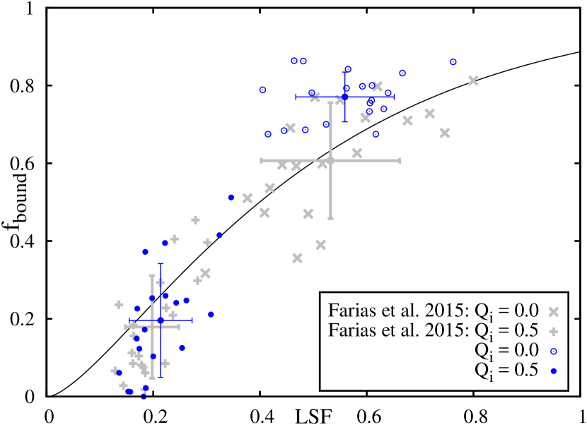
Figure 1: The $f_{\rm bound}$-LSF trend for fractal clusters embedded in a Plummer sphere of gas. Gray symbols are simulations with a static background potential (Farias et al., 2015) and blue symbols are simulations using a live gas background. In the simulations shown in this plot gas is expelled at the same dynamical time, i.e., when $Q=0.5$ and $Q$ is rising for the second time in the cluster evolution. Black line represents the Farias et al. (2015) model, i.e., Eq. 18 assuming $B/A=1$ (or $\eta=1/$LSF).

$\begin{array}[]{lr}\includegraphics[height=202.35622pt]{bafit}&\includegraphics[height=202.35622pt]{fixed_fb}\end{array}$

Figure 2: Left: The structural parameters $A$, $B$ and the ratio $B/A$ for simulations using a smooth live Plummer sphere as background. While $A$ is similar for simulations $B$ is highly dependent on the LSF where stars with low LSF are concentrated in the center and stars are not affected by the gas since most of it is outside the cluster. This dependency is reflected in the $B/A$ ratio and finally in the bound fraction of the cluster. We also show that the effective $Q_{\rm f}$ is another source of error in the $f_{\rm bound}$-LSF trend. To quantify the effect we show two fits to these parameters in a dashed green line for $B/A$ and a dotted blue line for the effective $Q_{\rm f}$. Right: We apply the previous fits showing that the particular shape of the $f_{\rm bound}$-LSF described in previous papers is a consequence of a combination of the particular geometry of the systems evolved and also our ability to measure $Q_{\rm f}$ correctly and is not necessarily a universal trend.

By using a smooth Plummer sphere of gas and expelling the gas when the systems have exactly $Q_{\rm f}=0.5$ we obtain the same trend as in Farias et al. (2015) (see Fig. 1). The main difference in both cases is a slight offset in the region of LSF that clusters populate. This is because if interactions between stars and gas are possible, stars loose energy in the interaction and sink to the center, raising the LSF. However, the change is not significant and the $f_{\rm bound}$-LSF trend is the same as in Farias et al. (2015).

Even though the trend is the same, it is quite obvious that the simple model of Farias et al. (2015) overestimates $f_{\rm bound}$ at low values of LSF ($\sim 0.2$) and the sample of live gas simulations appears to survive better than the model expects for LSF $>$ 0.4. We found two main reasons that give the $f_{\rm bound}$-LSF relation its particular shape. The first one is related to the basic assumptions in the model of Farias et al. (2015). To simplify the maths, it was assumed that the stars and gas are distributed in a similar way ($B/A\approx 1$). We make use of the structural parameters $A$ and $B$ to show how far simulations are from this assumption and also how much this affects the estimations. We note that we are not suggesting to measure such values in observable star clusters, and this is just an illustrative experiment. While the $A$ parameter is relatively similar for all simulations (top left panel in Fig.2), the $B$ parameter is highly dependent of how the stars are distributed inside the background gas (bottom left panel in Fig.2). We show the structural parameters as a function of the LSF. $A$ is similar for all the simulations since at that point the level of substructure and shape of the clusters are similar, however $B$ shows a strong dependency of the LSF. The reason is that at high LSFs stars are concentrated in the center and most of the gas is in the outer layers of the cluster (then $B$ is low). On the other hand, at low LSF the cluster is expanded and there is more gas inside the cluster ($B$ raises). Therefore, the ratio $B/A$ is highly dependent on the LSF (top middle panel), and thus Eqs. 10 and 18 imply that clusters survive better when $B/A<1$ and the opposite when $B/A>1$. We show a fit to this ratio (green dashed line in Fig. 2) and we show how this effect affects the model of Farias et al. (2015) in the right panel of Fig. 2 as the green dashed line. We see that this variation clearly explains the shape of the $f_{\rm bound}$-LSF trend at high LSF and also at low LSF. However, the effect of the LSF-dependent $B/A$-ratio is not strong enough to explain why star clusters don’t survive with LSFs below 0.2, as predicted by the Farias et al. (2015) analytical model.

	$R_{\rm h}$[pc]	LSF	$R_{\rm max}$[pc]	SFE${}_{R_{\rm max}}$	$\cal{C}$	$Q_{\rm i}$	$\sigma_{*}$[km/s]
Plummer Background
Cold	$0.9\pm 0.1$	$0.19\pm 0.03$	$1.5$	$0.2$	$0.39\pm 0.06$	$0.0$	$0$
Warm	$0.9\pm 0.1$	$0.19\pm 0.03$	$1.5$	$0.2$	$0.39\pm 0.06$	$0.5$	$1.0\pm 0.1$
Turbulent Setup
Divergence Free	$0.5\pm 0.3$	$0.6\pm 0.2$	$2.5\pm 0.9$	$0.24\pm 0.03$	$0.28\pm 0.07$	$0.31\pm 0.06$	$1.1\pm 0.2$
Mixed	$0.4\pm 0.3$	$0.6\pm 0.2$	$2.7\pm 0.9$	$0.23\pm 0.02$	$0.27\pm 0.08$	$0.31\pm 0.07$	$1.1\pm 0.2$
Curl Free	$0.6\pm 0.4$	$0.5\pm 0.2$	$2.5\pm 0.9$	$0.23\pm 0.03$	$0.24\pm 0.08$	$0.27\pm 0.06$	$0.9\pm 0.2$

Table 3: A comparison between the initial conditions generated by the turbulent setup and simulations with fractal distributions embedded in a Plummer background. Values are means with respective standard deviations for each set of simulations described in column 1. Column 2 shows the initial half mass radius of the stellar distribution in parsecs, column 3 the initial local stellar fraction, column 4 the radius containing all the stars in parsecs, column 5 the star formation efficiency measured at $R_{\rm max}$, column 6 the amount of primordial substructure measured by the $\cal C$ parameter, column 7 the initial virial ratio and column 8 the velocity dispersion of the stellar component.

The second reason of the particular shape of the trend is our ability to measure $Q_{\rm f}$. The virial ratio is highly dependent on the frame of reference. While the potential energy is not, the kinetic energy in the cluster is highly dependent of what we choose as the mean velocity of stars in the cluster. The simplest way is to use the mean velocity of the whole star distribution, and this generally works fine if we are in the ballpark of high LSF values. However, a more correct characteristic velocity for the cluster would be the mean velocity of only the stars that will actually remain bound. Of course we cannot know this last velocity since we would need to know exactly what particles will remain bound a priori. But we know that in general, when a high fraction (or at least representative) of the stars remains bound after gas expulsion, the mean velocity of the whole distribution is close enough to the velocity of the bound cluster, and the calculated $Q_{\rm f}$ is then representative. However, when $f_{\rm bound}$ is low, there is a lower chance that both velocities coincide. We call the virial ratio measured with the velocity of the stars that finally will remain bound the effective virial ratio. In reality, it is not possible to measure such value, but in our simulations we have all the information that we need to track the bound particles back and measure their mean velocity. The bottom middle panel on Fig. 2 shows the effective $Q_{\rm f}$ as a function of the LSF. At low LSFs, the velocity of the system is not representative of the one of the bound stars. While globally the star distributions have $Q_{\rm f}=0.5$ by design (see our criteria for the gas expulsion time), effectively the bound system has $Q_{\rm f}>0.5$ resulting in an over prediction of $f_{\rm bound}$. In order to illustrate how much the model of (Farias et al., 2015) is affected by these effects, we calculate the relation between LSF and $f_{\rm bound}$ with the fits shown in the middle panels of Figure 2 as inputs.

Both effects are important in different regimes, and the particular shape of the $f_{\rm bound}$-LSF trend is a combination of both. But more importantly, this simple fitting shows that the shape of the $f_{\rm bound}-LSF$ trend is not general and depends on how the stars and gas are distributed with respect to each other. Predicting the bound fractions seems to be quite a difficult task, especially if gas and stars remain substructured and have not had time to become a more spherical distributions, and also if the bound entity is small.

We will return to the topic of predicting the survivability of star clusters to instantaneous gas expulsion further down in the text. Here we want to stress that our simulations are designed to fully explore the parameter space in LSF and $Q_{\rm f}$ to be able to compare the analytical predictions to the complete trend obtained by our simulations. At this point, we are not concerned if the full parameter space extends beyond that inhabited by real star clusters, but we raise this issue again in the Discussion section.

4.2 Highly substructured gas distributions

As we describe in Section 3.3, we expel the gas of new born star clusters at three different times: Just after stars form (0 Myr) or after 1 or 2 Myr of embedded evolution. We follow the embedded evolution utilizing two very different treatments for the gas in order to avoid further collapse. Both approaches are likely unrealistic. However, they represent two extremes in the possible spatial distributions of the gas, that could have great relevance for the evolution of the stars after gas expulsion, since the gravitational potential fields that they produce are extremely different. We will avoid the discussion of which scenario is closer to reality for now. We emphasize the objective of the simulations presented in this work are rather illustrative, to show the effects of large variations in the background substructure, rather than to attempt to match the background substructure found in real star clusters.

4.2.1 The new initial conditions

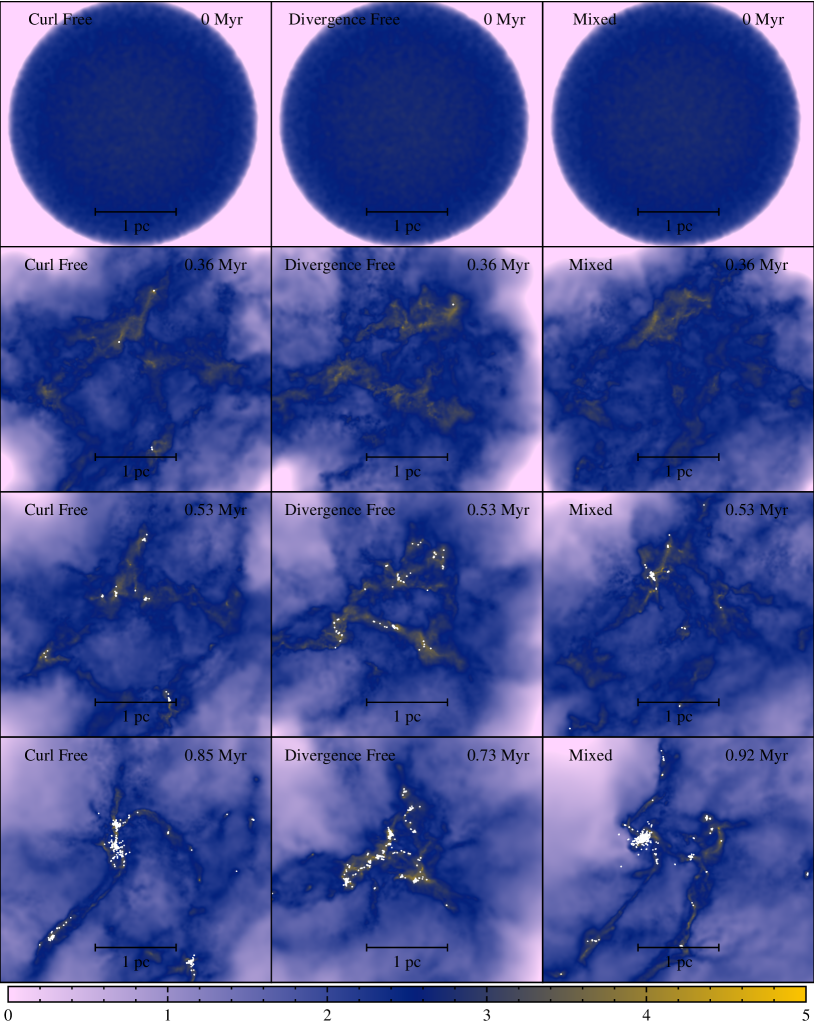
Figure 3: Evolution of the initially homogeneous turbulent molecular clouds until $N=1000$ equal mass stars are formed. Simulations with curl-free (left column), divergence-free (middle column) and mixed (right column) turbulent fields are shown at (from top to bottom panels) 0 Myr, 0.36 Myr, 0.56 Myr and when 1000 stars are formed using the same random seed. Each panel has $3\times 3$ pc² and the color bar represent the logarithmic column density measured in $\rm{~{}M}_{\odot}$/pc². This figure, as well as the others column density figures in this work, have been prepared with the Splash tool developed by Price (2011).

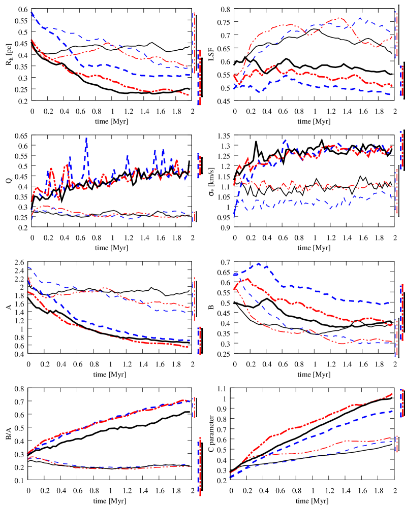
Figure 4: The evolution of the embedded star clusters for 2 Myr after the $N=1000$ stars form. Values are means for each parameter of the 10 realizations for each setup where standard deviations been omitted for clarity. From top to bottom and left to right: The stellar half mass radius $R_{\rm h}$, the Local Stellar Fraction, the virial ratio $Q$, the stellar velocity dispersion $\sigma_{*}$, the structure parameters $A$ and $B$, the $B/A$ ratio and the $\cal C$ parameter. Thick lines are AEOS simulations and thin lines are SGO simulations. In both cases divergence free setup is shown in a dot dashed red line, curl-free in a dashed blue line and mixed setup in solid black lines. The standard deviation on each ensemble is averaged over time and shown at the right of each panel to represent a typical error. We advise to the reader to pay attention to the minimum and maximum values of the y axes on the different panels.

The nature of the initial velocity field has a strong consequence in the substructure formed by the gas. While compressive motions tend to form large voids and filaments, solenoidal velocity fields tend to form a more uniform substructure (see e.g. Federrath et al., 2009). Hence, we split our simulations in three groups depending of the initial velocity field: the compressive (curl free), solenoidal (divergence free) and mixed velocity fields. Fig. 3 shows snapshots at different times of the three kinds of simulations until the end of the star formation phase.

We attempt to form systems similar to the ones in our first experiment with a Plummer Sphere of gas. Table 3 shows a summary of some important parameters that we compare with the initial conditions of simulations using a smooth background gas.

To measure the level of substructure we make use of the $\cal C$ parameter introduced by Cartwright & Whitworth (2004) which is the ratio between the area normalized mean length of a minimum spanning tree joining all the particles ($\bar{m}$) and the area normalized mean separation between particles. Values of ${\cal C}<0.8$ are obtained in fractal-like stellar distribution (where a lower $\cal C$ is obtained with smaller fractal dimensions, i.e. high level of substructure) and ${\cal C}>0.8$ is obtained in spherical distributions where a higher value of $\cal C$ matches a steeper density profile.

Even though there is a big difference between the substructure of the gas generated by either a curl-free or divergence-free velocity field, this is not expressed in the resulting stellar distributions where the resulting level of substructure is very similar in all cases. This is because stars and gas quickly decouple, and stars tend to form their own independent distribution through mergers of sub-groups. This similarity is in agreement with Lomax et al. (2015) and Girichidis et al. (2012), where the same turbulent modes where tested. We obtain the same slight difference in the mean values of $\cal C$ as Girichidis et al. (2012), with $\left\langle{\cal C}_{\rm comp}\right\rangle\lesssim\left\langle{\cal C}_{\rm mix}\right\rangle\lesssim\left\langle{\cal C}_{\rm sol}\right\rangle$. However, the differences are very small and well within the standard errors.

We obtain even more substructured star clusters than the $D_{\rm f}=1.6$ fractals used in our previous studies, with ${\cal C}\sim 0.26$, comparable to fractal distributions with $D_{\rm f}<1.5$.

In comparison with the initial conditions used in our previous studies, we now form clusters with 2.5 pc radius and SFE $\sim$ 24%. This is slightly higher than the setup SFE of 20%, since there is always some gas outside the maximum radius of the cluster $R_{\rm max}$. Distributions using the turbulent setup form with a higher LSF. This is a consequence of the shape of the gas, which is distributed in filaments around the cluster rather than concentrated in the center of the stellar distribution. Furthermore, we obtain smaller half mass radii meaning that in general our stellar distributions are more centrally concentrated in comparison with the fractal method described by Cartwright & Whitworth (2004).

4.2.2 Embedded evolution

The embedded evolution strongly depends on the numerical treatment of the gas, or more accurately, on the behaviour of the gas. It is important to know how the star clusters behave under different background gas conditions since this determines their matter distribution and dynamical state at the time of gas expulsion.

Fig. 4 shows time evolution of the mean stellar values for the different sets that expel the gas at 2 Myr of embedded evolution. Note that the initial conditions for the AEOS and the SGO simulations are the same for each turbulent setup, and differences only depend on the background gas.

In AEOS simulations (thick lines) gas quickly forms clumps which, as a difference with an isothermal EOS, are thermal pressure supported. Anywhere a overdensity exists at the end of the star formation phase, changing the EOS to adiabatic causes the gas to quickly form roughly spherical gas clumps in internal equilibrium that later merge into larger clumps. The stars follow the potential generated by these clumps causing the star cluster half mass radius to decrease (first row, left panel), however the LSF remains roughly constant and does not rise like in the static background case (first row, right panel), since gas is also being concentrated in the center. Interactions caused by the mergers help the star cluster to reach equilibrium, as we can see in the $Q$ panel of Fig. 4 (second row, left panel) the virial ratio increases roughly linearly and usually 2 Myr are enough for these star clusters to reach equilibrium. In contrast, in SGO simulations (thin lines) gas disperses instead of forming clumps, overdensities are not so strong and stars do not have a clearly defined potential where to merge. Therefore, the local free fall time, and also the crossing time of the region (since stars have small velocities; see second row, right panel) is longer and thus the timescale that the cluster needs to virialize is longer. As consequence, stars do not have time to virialize in the 2 Myr that we evolve the embedded phase.

Despite those differences, the strength of the potential field generated by the gas is quite similar (see parameter $B$ in Fig. 4; third row, right panel), with the AEOS simulations being stronger, however the big difference we can appreciate in the $B/A$ ratio (fourth row, left panel) comes from how the stars rearrange in both scenarios. The parameter $A$ (third row, left panel) summarizes the strength of the potential generated by the stars and decreases with time for the AEOS simulations, this is a consequence of erasing the substructures. At 0 Myr, stars are distributed in a fractal-like substructure and stars are generally very close to each other in comparison with the volume of the sphere that contains them. This raises the potential energy of the stars, however, in AEOS simulations substructure is erased very quickly due to mergers (as we can see in the $\cal C$ parameter panel of Fig. 4; fourth row right panel). When substructure is erased the stellar distribution spreads over the volume decreasing the value of $A$. Even though we can see that substructure of the SGO simulations also decreases ($\cal C$ raises), the $\cal C$ parameter never reach the ${\cal C}=0.8$ limit that split spherical distributions from substructured distributions, and $A$ decreases very slowly.

As we see in section 2.1, star cluster survivability depends on $Q$ and the $B/A$ ratio, which never reach values above 1 in these simulations, meaning that they can survive better. Considering also the low values of $Q$ for the SGO simulations, the simulated star clusters are likely to be able to easily survive gas expulsion. We will analyse the outcomes of gas expulsion in the next section.

4.2.3 Survival to gas expulsion

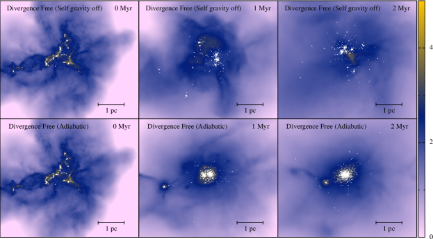
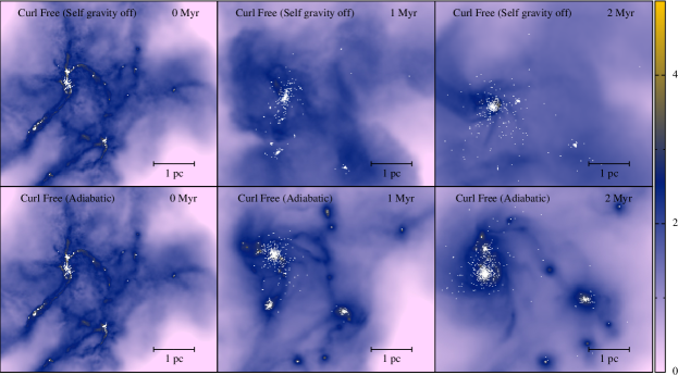
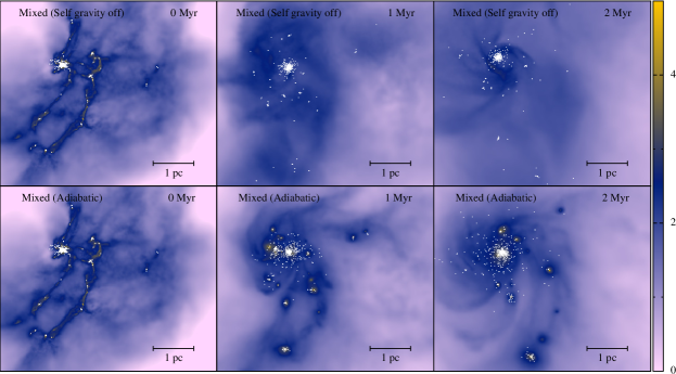
Figure 5: Example snapshots of embedded star clusters with each initial turbulent velocity field at the times when gas is expelled. Top panels of each 6 panel sets, shows the evolution of the cluster when self-gravity of the gas is turned off (SGO simulations), bottom panels show the same distribution but evolving under an adiabatic EOS for the gas (AEOS simulations). Colors represent the Logarithm of the column density measured in $\rm{~{}M}_{\odot}$/pc².

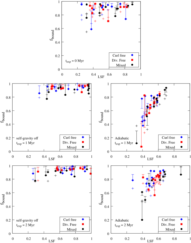
Figure 6: Bound fractions for embedded star clusters at 15 Myr from the moment of gas expulsion. Different panels show sets of simulations expelling the gas at 0 Myr (top panel), 1 Myr (middle panels) and 2 Myr (bottom) after the end of the star formation phase. Panels at the left are the results from SGO simulations and right panels show the resulting bound fractions from AEOS simulations. The different natal velocity fields are shown as different symbols with curl-free velocity fields in blue diamonds, divergence free fields in red squared and the mixture of both in black circles. Error bars show the prediction of the model presented in this work taking into account the substructure of the gas and the stars through the parameters $A$ and $B$. Crosses are the predictions of the model without considering substructure as described in (Farias et al., 2015), i.e., assuming $B/A=1$. All model predictions are calculated using the effective $Q_{\rm f}$ discussed in Sec. 4.1.

We expel the gas in the cluster at three different times after the embedded phase starts, at the beginning (0 Myr), at 1 and at 2 Myr. Then we measure the bound fraction after 15 Myr of gas free evolution. Fig. 5 shows snapshots of one of our simulations for each of the initial turbulent fields and numerical treatment of the background gas at the moment of gas expulsion, so that we can clearly see the level of remaining substructure in the gas and stars at each stage. Fig. 6 shows the results of the bound fraction measurement after 15 Myr of gas expulsion for each set. We include the predictions of the analytical model described in section 2.1, which accounts for the independent substructure of the stars and gas as error bars (i.e. Eq. 18). We also show the prediction of the analytical model introduced in Farias et al. (2015), which assumes a identical distribution of mass for the stars and the gas (i.e. Eq. 18 assuming $B/A=1$). All predictions shown in Fig. 6 are deduced using the effective $Q_{\rm f}$ discussed in section 4.1, however, this choice is not very important as we will see later in this section.

The high survival rates of simulations expelling the gas at 0 Myr and the SGO simulations are mainly explained by the low virial ratios that the stars have and their inability to reach virial equilibrium. The SGO simulations also have very low $B/A$ ratios, so in general they survive gas expulsion remarkably well. The AEOS simulations show a trend very similar to the Plummer background case presented in Section 4.1. The gas quickly rearranges into a spherical distribution and the stars follow the potential well generated by the gas, forming (in general) a similar configuration than the Plummer background case. In this last scenario stars also have the chance to reach virial equilibrium velocities and in general they are quite virialized in comparison to the SGO simulations by the time we expel the gas.

The disagreement between the model introduced in Section (2.1) and the numerical simulations is represented by the error bars in Figure 6. This reveals that the model introduced in Section 2.1 does a good job at predicting the bound fraction (i.e. the error bars are small). It is, however, remarkable that its performance predicting bound fractions is not always better than the simple $B/A=1$ model. Thus, everything seems to be fairly well explained when measuring the effective $Q_{\rm f}$ and the consideration of substructure does not improve the predictions significantly. And, as we will see later, even if we do not use the effective $Q_{\rm f}$, predictions are still good without considering the substructure.

We also test the alternative approach described in Section 2.2. Since Eq. 21 only depends on one parameter, the immediately post gas expulsion virial ratio $Q_{\rm a}$ we put the results of all the simulations performed in this work into Fig. 7. $Q_{\rm a}$ works quite well when estimating $f_{\rm bound}$ and it has the advantage that it does not depend of the background gas, all we need is accurate information of the positions and velocities of the stars alone (assuming instantaneous gas expulsion).

In order to quantify the performance of different analytical models, we measure the difference of the measured $f_{\rm bound}$ with the estimated $f_{\rm bound}$ and we calculate the standard error for all the simulations performed in this paper. We consider six flavours of the analytical models introduced in Section 4 and in Farias et al. (2015). These six flavours come about by considering three sets, namely one set where substructure is ignored (i.e. $B/A=1$), one set where the substructure is measured through the parameters $A$ and $B$, and one set where the clusters are characterized by their $Q_{\rm a}$. For each of these three sets, we consider both the global $Q_{\rm f}$ and the effective $Q_{\rm f}$ as described in Section 4.1. We show the resulting residuals in Fig. 8 where shadow areas show the standard deviation from the models.

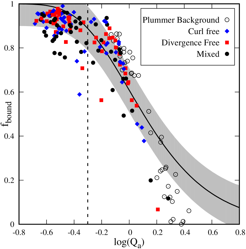
Figure 7: The post-gas expulsion virial ratio $Q_{\rm a}$ as an estimator of $f_{\rm bound}$ for all the simulations performed in this study. Black solid line is the prediction of Eq. 21 which is not dependent on the geometry of the system, with gray areas as the standard deviation from the curve. Values of $Q_{\rm a}$ are effective values. Vertical dashed line represents $Q_{\rm a}=0.5$ for reader’s reference.

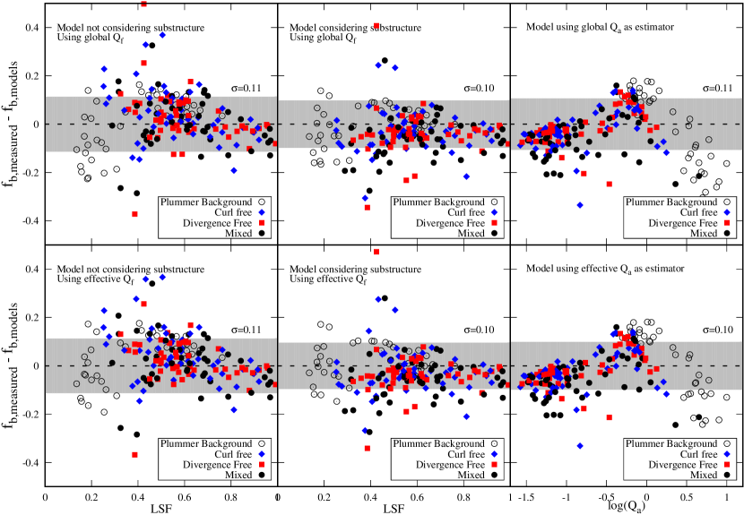
Figure 8: The differences between the analytic models and the measured bound fractions for all the simulations performed in this paper. Top panels show the performance of the models when measuring $Q_{\rm f}$ with respect to the global mean velocity while bottom panels show the performance of the models when measuring the effective $Q_{\rm f}$ i.e. when using the mean velocity of the clump that remains bound after gas expulsion (see section 4.1). Left panels show the behaviour of the models when we do not take into account structure parameters (assuming $B/A=1$). Middle panels shows results when substructure is included through the measure of the parameters $A$ and $B$ and right panels shows the performance of the model when using $Q_{\rm a}$ as estimator of $f_{\rm bound}$ (see Eq. 21). Different natal velocity fields are shown in the same way than in Figs. 6 and 7. Simulations with a Plummer background gas (see Fig. 2) are shown as black open circles. We measure the performance of the analytical models through the standard deviation from the models represented by the gray shaded areas. We can see that the consideration of the effective $Q_{\rm f}$ does not change the performance (due to the generally big $f_{\rm bound}$ obtained in this work) and the consideration of substructure only improves the accuracy of the models on a 1 percentage point level. The use of $Q_{\rm a}$ does not improve the estimations either. We show that we can predict the outcome of all the simulations in this work with 10 percentage points uncertainly even in cases of high levels of substructure in the gas and stars.

There is a remarkable agreement in the predictions between the different analytical models, no matter if we measure substructure effects or not. In all cases the accuracy of the predictions are of order of 10 percentage points. When carefully measuring the effects of independent substructure, predictions only improve by 1 percentage point. Using the effective or the global $Q$ does not improve the estimations significantly. However, this is because we obtain, in general, high $f_{\rm bound}$ values for simulations in the turbulent setup, where the difference between global and effective $Q$ is minimal, i.e., the mean velocity of the bound entity is similar to the whole cluster when $f_{\rm bound}$ is big since the bound entity is a considerably large subset of the cluster.

By eye it appears that there is some improvement from the left panel of Fig. 8 to the middle and right panels, however this is not reflected in the standard errors.

The results show that the inclusion of an arbitrary distribution for the gas and the stars does not result in an unpredictable scenario. In fact, the results suggest that it is possible to estimate how much mass a cluster can retain in any distribution if it is possible to measure at least the virial ratio of the stellar distribution, without caring for the presence of substructure or even for the background gas.

5 Discussion and Conclusions

We have introduced a simple analytical model that estimates the amount of mass a star cluster can retain if we instantaneously remove the remaining gas. We have presented this model in three flavours: By assuming equal distributions for the gas and the stars, by carefully measuring the effects of the independent substructure of the gas and stars, and by only considering the dynamical state of the cluster right after gas is expelled. We have tested our analytical model by conducting simulations of instantaneous gas expulsion in highly substructured, embedded star clusters. The amount of substructure present at the time of gas expulsion was varied in a controlled manner by varying the treatment of the background gas.

We find, independent of the treatment of the background gas, the most important parameters to estimate the survival of a cluster to gas expulsion are the LSF and the virial ratio at the moment of gas expulsion. However, we also introduce another independent parameter that works equally well – the post-gas-expulsion virial ratio. As we are dealing with instantaneous gas expulsion, this is effectively the same as the pre-gas-expulsion ratio if we only consider the contribution from the stars, and we disregard the gas contribution altogether. The main advantage of $Q_{\rm a}$ is that we only need information about the stars, ignoring completely the presence of the gas.

The three flavours of the model presented in this paper work equally well in most cases, estimating final bound fractions with a standard error of $\sim$ 10 percentage points. The models are not reliable when the bound fractions are low ($\lesssim 40\%$), not because the models are wrong, but because of technical difficulties when measuring an accurate virial ratio. An accurate measure of such a value involves information about the individual members of the cluster that will remain bound after gas expulsion, which is the information we are trying to estimate in the first place. Or in other words, it is more or less impossible to describe the behaviour of a small sub-set of stars by using global parameters determined using all the stars.

However, we find it very difficult to obtain low values of $f_{\rm bound}$ when testing our models in the more “realistic” gas distributions.

Our more “realistic” embedded star clusters are obtained from star formation simulations that arguably are very simplistic but are in agreement with other more sophisticated simulations: stars form with sub-virial velocities in fractal-like structures that initially follow the gas distribution, but stars quickly decouple from the gas during the star cluster formation, trying to form their own independent distribution. We find that this mode of star cluster formation is quite stable against gas removal. Decoupling from the gas keeps the LSF high and their low stellar velocities remain low during the star cluster formation process.

We also follow the evolution of the embedded star cluster after stars form. We find that the behaviour of the gas during this phase is critical to “prepare” the cluster for gas expulsion. We test two extremes of gas evolution: As a first attempt, we stop gravitational collapse of the gas by switching the equation of state of the gas from isothermal to adiabatic. This scenario quickly forms clumps of stars that merges into bigger clumps and stars couple again with the gas following the overdensities. As an alternative approach, we just switch off the self gravity of the gas. In this case gas disperses around the cluster and stars and gas remain decoupled since there are no significant overdensities to follow. We obtain completely different results in both cases since, in the first case, the system tends to form a spherical cluster just like in our previous studies reaching virial equilibrium in the process. In the second case, substructure is not erased so efficiently and stars do not have the chance to merge and virialize in the 2 Myr that we follow their evolution. Therefore, velocities remain low at all times in this scenario, and star clusters are able to retain at least $\sim 80\%$ of their mass.

While it can be argued that both scenarios are completely unphysical, we wish to note that reality may be in between. The equation of the state of the gas in the embedded phase is not completely understood yet, as it involves complex heating processes. However, after stars are formed, it is very unlikely that gas is able to accumulate inside the stellar distribution since radiation from stars would quickly disperse the interior gas. The scenario (in terms of spatial distribution) may be similar to the second case when we turned off the gravity of the gas. Stars will give enough energy to the gas to support and overcome the gravitational collapse. If further overdensities form, they will form more likely outside the star cluster, and therefore will not contribute to the gravitational potential of the stellar cluster. The reader should also keep in mind that all our results are a lower limit of cluster survival. We use instantaneous gas expulsion which is the most destructive mode of gas expulsion. The timescales of gas expulsion are not known yet, but they cannot be more destructive than the description used in this study.

Our results are in close agreement with a similar study realized by Kruijssen et al. (2012), who analyzed the outcome of the hydrodynamical simulations performed by Bonnell et al. (2003, 2008) studying the dynamical state of sub-clusters in the simulations. They found that stars are formed sub-virial even when ignoring the background gas and gas fractions inside sub-clusters are small enough to enable stellar sub-clusters to remain bound when gas is expelled, even in absence of stellar feedback. Lee & Goodwin (2016) have also noted that the virial ratio is the only relevant parameter when estimating bound fractions. Our study compliments this conclusions by adding that the gas fraction inside the stellar component is not crucial, as long as the stars are able to remain sub-virial during the embedded phase. This is likely to happen if the gas does not form strong overdensities, e.g. is being dispersed, or when stellar substructure in the star forming region is still important.

We, therefore, can summarize our main conclusions as follows:

1. Accurate estimations of the maximum amount of mass that a cluster will loose in the transition from the embedded phase to the gas free phase are possible by measuring the dynamical state of the stellar component alone ($Q_{\rm a}$), i.e., ignoring the presence of the gas.

2. Star clusters formed with low initial velocities are likely to remain in a sub-virial state for long time. If the gas is not able to concentrate and form considerable overdensities, then stellar substrucutre lasts longer.

3. Since erasure of substructure is accompanied by virialization, we find that star clusters with high levels of substructure are quite stable against gas expulsion no matter how high the gas fraction inside the stellar distribution is.

The first result make estimations on observable embedded star clusters easier since estimations of the potential energy from molecular clouds are highly challenging. We emphasize that it is possible to just ignore the gas to estimate how bound the cluster is. Considering that there is theoretical and observable evidence that star clusters form in sub-virial states (e.g., Bonnell et al., 2003, 2008) and that feedback would keep the gas disperse inside the stellar clusters (if present at all, see Kruijssen et al., 2012) then the conditions in young star clusters are such that they are very likely to survive gas expulsion, and therefore gas expulsion may not be the culprit for infant mortality.

Appendix A Resolution criteria for Plummer gas background simulations

In SPH, a continuum of gas is transformed into a set of smoothed particles with a certain smoothing length $h_{i}$. Stars traveling through this sea of particles can be unphysically deflected when gravitationally interacting with these particles. The critical velocity at which a star is considerably deflected in our Plummer gas background setup is

$$v_{\rm crit} = \sqrt{\frac{2GM_{\rm pl}}{N_{\rm gas}h_{i}}}$$ (23)

(see Hubber et al., 2013), and therefore the velocity dispersion of the stars must be much larger than $v_{\rm crit}$.

Hubber et al. (2013) developed a resolution criterion for the same experiment we are exploring, but in a different implementation of the SPH technique. In this section, we apply this criterion to the grad-SPH implementation used in this work.

In the current implementation of the SPH technique, $h_{i}$ is obtained by solving the equation

$$\frac{4\pi}{3}h_{i}^{3}(\rho_{i}+\rho_{\rm min})-N_{\rm nb}\langle m_{i}\rangle = 0$$ (24)

(Pelupessy, 2005), where $N_{\rm nb}$ is the target number of neighbours, $\rho_{\rm min}$ is a small density threshold to avoid excessive large $h_{i}$ at the edges of the simulation and $\langle m_{i}\rangle$ is the mean mass of the SPH particles, in our case this is simply $\langle m_{i}\rangle=M_{\rm pl}/N_{\rm gas}$.

The smallest value of $h_{i}$ – the place with larger $v_{\rm crit}$ – is the central region of the Plummer sphere where we have:

$$\rho_{\rm max} \approx \frac{3M_{\rm pl}}{4\pi R_{\rm pl}^{3}}.$$ (25)

The smallest $h_{i}$ is then

$$h_{\rm min} \approx \left(\frac{N_{\rm nb}}{N_{\rm gas}}\right)^{1/3}R_{\rm pl},$$ (26)

where we have neglected the contribution of $\rho_{\rm min}$.

Assuming a spherical Plummer-like stellar distribution, the velocity dispersion in the central region of the gas-star system is

$$\sigma_{\rm c} \approx \sqrt{\frac{1}{6(1-{\rm SFE})}\frac{GM_{pl}}{R_{\rm pl}}},$$ (27)

where $M_{\rm pl}/(1-{\rm SFE})=M_{\rm tot}$, i.e. the total mass in the cluster.

Then, the resolution criteria $\sigma_{\rm c}/v_{\rm crit}\gg 1$ becomes:

$$\sqrt{\frac{N_{\rm nb}^{1/3}}{12(1-{\rm SFE})}}N_{\rm gas}^{1/3} \gg 1.$$ (28)

In the Plummer gas background simulations performed in this work we have used $N_{\rm gas}=100$K, $N_{\rm nb}=64$ and SFE$=0.2$ and the factor $\sigma_{\rm c}/v_{\rm crit}=30.0$, which is enough to avoid numerical scattering. We note that this factor does not increase considerably if $N_{\rm gas}$ increases. As shown by Hubber et al. (2011), a few thousand particles is enough to accurately reproduce an equilibrium polytrope.

References

- Barnes & Hut (1986) Barnes J., Hut P., 1986, Nature, 324, 446
- Bastian & Goodwin (2006) Bastian N., Goodwin S. P., 2006, MNRAS, 369, L9
- Bate (2009) Bate M. R., 2009, MNRAS, 392, 590
- Bate et al. (2002) Bate M. R., Bonnell I. A., Bromm V., 2002, MNRAS, 332, L65
- Baumgardt & Kroupa (2007) Baumgardt H., Kroupa P., 2007, MNRAS, 380, 1589
- Boily & Kroupa (2003a) Boily C. M., Kroupa P., 2003a, MNRAS, 338, 665
- Boily & Kroupa (2003b) Boily C. M., Kroupa P., 2003b, MNRAS, 338, 673
- Bonnell et al. (2003) Bonnell I. A., Bate M. R., Vine S. G., 2003, MNRAS, 343, 413
- Bonnell et al. (2008) Bonnell I. A., Clark P., Bate M. R., 2008, MNRAS, 389, 1556
- Bressert et al. (2010) Bressert E., et al., 2010, MNRAS, 409, L54
- Cartwright & Whitworth (2004) Cartwright A., Whitworth A. P., 2004, MNRAS, 348, 589
- Dobbs et al. (2014) Dobbs C. L., et al., 2014, Protostars and Planets VI, pp 3–26
- Elmegreen (1983) Elmegreen B. G., 1983, MNRAS, 203, 1011
- Elmegreen & Clemens (1985) Elmegreen B. G., Clemens C., 1985, ApJ, 294, 523
- Farias et al. (2015) Farias J. P., Smith R., Fellhauer M., Goodwin S., Candlish G. N., Blaña M., Dominguez R., 2015, MNRAS, 450, 2451
- Federrath et al. (2009) Federrath C., Klessen R. S., Schmidt W., 2009, ApJ, 692, 364
- Fujii et al. (2007) Fujii M., Iwasawa M., Funato Y., Makino J., 2007, PASJ, 59, 1095
- Gerritsen & Icke (1997) Gerritsen J. P. E., Icke V., 1997, A&A, 325, 972
- Geyer & Burkert (2001) Geyer M. P., Burkert A., 2001, MNRAS, 323, 988
- Girichidis et al. (2012) Girichidis P., Federrath C., Allison R., Banerjee R., Klessen R. S., 2012, MNRAS, 420, 3264
- Goodwin (1997a) Goodwin S. P., 1997a, MNRAS, 284, 785
- Goodwin (1997b) Goodwin S. P., 1997b, MNRAS, 286, 669
- Goodwin (2009) Goodwin S. P., 2009, Ap&SS, 324, 259
- Goodwin & Bastian (2006) Goodwin S. P., Bastian N., 2006, MNRAS, 373, 752
- Goodwin & Whitworth (2004) Goodwin S. P., Whitworth A. P., 2004, A&A, 413, 929
- Gutermuth et al. (2009) Gutermuth R. A., Megeath S. T., Myers P. C., Allen L. E., Pipher J. L., Fazio G. G., 2009, ApJS, 184, 18
- Heitsch et al. (2001) Heitsch F., Mac Low M.-M., Klessen R. S., 2001, ApJ, 547, 280
- Hernquist & Katz (1989) Hernquist L., Katz N., 1989, ApJS, 70, 419
- Hills (1980) Hills J. G., 1980, ApJ, 235, 986
- Hubber et al. (2006) Hubber D. A., Goodwin S. P., Whitworth A. P., 2006, A&A, 450, 881
- Hubber et al. (2011) Hubber D. A., Batty C. P., McLeod A., Whitworth A. P., 2011, A&A, 529, A27
- Hubber et al. (2013) Hubber D. A., Allison R. J., Smith R., Goodwin S. P., 2013, MNRAS, 430, 1599
- Johnstone et al. (2000) Johnstone D., Wilson C. D., Moriarty-Schieven G., Joncas G., Smith G., Gregersen E., Fich M., 2000, ApJ, 545, 327
- King et al. (2012) King R. R., Goodwin S. P., Parker R. J., Patience J., 2012, MNRAS, 427, 2636
- Kirk et al. (2007) Kirk H., Johnstone D., Tafalla M., 2007, ApJ, 668, 1042
- Klessen & Burkert (2000) Klessen R. S., Burkert A., 2000, ApJS, 128, 287
- Klessen et al. (1998) Klessen R. S., Burkert A., Bate M. R., 1998, ApJ, 501, L205
- Könyves et al. (2010) Könyves V., et al., 2010, A&A, 518, L106
- Kruijssen et al. (2012) Kruijssen J. M. D., Maschberger T., Moeckel N., Clarke C. J., Bastian N., Bonnell I. A., 2012, MNRAS, 419, 841
- Krumholz & Tan (2007) Krumholz M. R., Tan J. C., 2007, ApJ, 654, 304
- Lada & Lada (2003) Lada C. J., Lada E. A., 2003, ARA&A, 41, 57
- Lada et al. (1984) Lada C. J., Margulis M., Dearborn D., 1984, ApJ, 285, 141
- Lee & Goodwin (2016) Lee P. L., Goodwin S. P., 2016, MNRAS, 460, 2997
- Li et al. (2003) Li Y., Klessen R. S., Mac Low M.-M., 2003, ApJ, 592, 975
- Lomax et al. (2015) Lomax O., Whitworth A. P., Hubber D. A., 2015, MNRAS, 449, 662
- Mac Low & Klessen (2004) Mac Low M., Klessen R. S., 2004, Reviews of Modern Physics, 76, 125
- Makino & Aarseth (1992) Makino J., Aarseth S. J., 1992, PASJ, 44, 141
- Mathieu (1983) Mathieu R. D., 1983, ApJ, 267, L97
- Maury et al. (2011) Maury A. J., André P., Men’shchikov A., Könyves V., Bontemps S., 2011, A&A, 535, A77
- McMillan et al. (2012) McMillan S., Portegies Zwart S., van Elteren A., Whitehead A., 2012, in Capuzzo-Dolcetta R., Limongi M., Tornambè A., eds, Astronomical Society of the Pacific Conference Series Vol. 453, Advances in Computational Astrophysics: Methods, Tools, and Outcome. p. 129 (arXiv:1111.3987)
- Monaghan & Lattanzio (1985) Monaghan J. J., Lattanzio J. C., 1985, A&A, 149, 135
- Padoan et al. (2014) Padoan P., Federrath C., Chabrier G., Evans II N. J., Johnstone D., Jørgensen J. K., McKee C. F., Nordlund Å., 2014, Protostars and Planets VI, pp 77–100
- Parmentier et al. (2008) Parmentier G., Goodwin S. P., Kroupa P., Baumgardt H., 2008, ApJ, 678, 347
- Pelupessy (2005) Pelupessy F. I., 2005, PhD thesis, Leiden University, Leiden Observatory
- Pelupessy & Portegies Zwart (2012) Pelupessy F. I., Portegies Zwart S., 2012, MNRAS, 420, 1503
- Pelupessy et al. (2004) Pelupessy F. I., van der Werf P. P., Icke V., 2004, A&A, 422, 55
- Pelupessy et al. (2013) Pelupessy F. I., van Elteren A., de Vries N., McMillan S. L. W., Drost N., Portegies Zwart S. F., 2013, A&A, 557, A84
- Pinto (1987) Pinto F., 1987, PASP, 99, 1161
- Portegies Zwart et al. (2013) Portegies Zwart S., McMillan S. L. W., van Elteren E., Pelupessy I., de Vries N., 2013, Computer Physics Communications, 183, 456
- Price (2011) Price D. J., 2011, SPLASH: An Interactive Visualization Tool for Smoothed Particle Hydrodynamics Simulations, Astrophysics Source Code Library (ascl:1103.004)
- Price & Bate (2009) Price D. J., Bate M. R., 2009, MNRAS, 398, 33
- Schmeja et al. (2008) Schmeja S., Kumar M. S. N., Ferreira B., 2008, MNRAS, 389, 1209
- Smith et al. (2011) Smith R., Fellhauer M., Goodwin S., Assmann P., 2011, MNRAS, 414, 3036
- Smith et al. (2013a) Smith R., Goodwin S., Fellhauer M., Assmann P., 2013a, MNRAS, 428, 1303
- Smith et al. (2013b) Smith R., Sánchez-Janssen R., Fellhauer M., Puzia T. H., Aguerri J. A. L., Farias J. P., 2013b, MNRAS, 429, 1066
- Springel & Hernquist (2002) Springel V., Hernquist L., 2002, MNRAS, 333, 649
- Tutukov (1978) Tutukov A. V., 1978, A&A, 70, 57