Strange stars in Krori-Barua spacetime under $f(R,T)$ gravity

Abstract

In the present work, we study about highly dense compact stars which are made of quarks, specially strange quarks, adopting the Krori-Barua (KB) [1] metric in the framework of $f(R,T)$ gravity. The equation of state (EOS) of a strange star can be represented by the MIT bag model as $p_{r}(r)=\frac{1}{3}[\rho(r)-4B_{g}]$ where $B_{g}$ is the bag constant, arises due to the quark pressure. Main motive behind our study is to find out singularity free and physically acceptable solutions for different features of strange stars. Here we also investigate the effect of alternative gravity in the formation of strange stars. We find that our model is consistent with various energy conditions and also satisfies Herrera’s cracking condition, TOV equation, static stability criteria of Harrison-Zel^′dovich-Novikov etc. The value of the adiabatic indices as well as the EOS parameters re-establish the acceptability of our model. Here in detail we have studied specifically three different strange star candidates, viz. $PSRJ~{}1614~{}2230,Vela~{}X-1$ and $Cen~{}X-3$. As a whole, present model fulfils all the criteria for stability. Another fascinating point we have discussed is the value of the bag constant which lies in the range $(40-45)$ MeV/fm³. This is quite smaller than the predicted range, i.e., $(55-75)$ MeV/fm³  [2, 3]. The presence of the constant ($\chi$), arises due to the coupling between matter and geometry, is responsible behind this reduction in $B_{g}$ value. For $\chi=0$, we get the higher value for $B_{g}$ as the above mentioned predicted range.

H I G H L I G H T   $\bullet$ We study anisotropic strange star in $f(R,T)$ gravity under Krori-Barua spacetime.

$\bullet$ The set of solutions provides non-singular as well as stable stellar model.

$\bullet$ Using observed values for mass and radius, we calculate different physical parameters.

$\bullet$ The coupling constant $\chi$, between matter and geometry, is the key factor in $f(R,T)$ gravity.  

1 Introduction

At the final stage of a gravitationally collapsed star, i.e., when all the thermonuclear fuels get exhausted it turns into a neutron star. In the year 1932, the particle neutron was discovered by Chadwick and soon after this discovery the actuality of neutron star was predicted. Later, this concept was strongly confirmed through the observational evidences from pulsars [4].

The density of neutron stars is enormously high that can bend the spacetime fabric, mostly dominated by neutrons along with a negligible fraction of electrons and protons. Neutron star is very small in expanse, radius of it extends upto 11 to 15 km [5] and mass about 1.4 to 2 solar mass ($M_{\odot}$) [5]. So the baryon density in a neutron star is extremely high and more than the nuclear saturation density $n_{S}\approx 0.16fm^{-3}$ (where nucleons start striking one another) depending on the explicit object. But the calculations show that the density at the centre of any massive neutron star becomes four or more times greater than the nuclear saturation density. This emphasizes regarding the high probability of a neutron star to deconfine into a quark-gluon plasma.

Due to enormous density, the energy level of the hyperon at the Fermi-surface becomes higher than its rest mass. This phenomenon indicates that these particles could deconfine into strange quarks which are the most stable quarks and form strange stars. Strange stars are basically consist of up $(u)$, down $(d)$ and strange $(s)$ quarks but mostly dominated by strange $(s)$ quarks. There are examples of potential candidates for strange stars available in the literature such as $SAX~{}J~{}1808.4-3658(SS2),SAX~{}J~{}1808.4-3658(SS1)$, X-ray binaries at low mass as $4U~{}1820-30$ etc.

In this connection we represent the equation of state (EOS) for a strange star as

$$p_{r}(r)=\frac{1}{3}\left[\rho(r)-4B_{g}\right],$$ (1)

which is known as the bag model (as proposed by MIT group) where $B_{g}$ is the bag constant. There are many literatures  [6, 7, 8, 9, 10, 11, 12, 13] available based on MIT bag model EOS for studying the strange stars and their stellar structures on the background of Einstein’s general theory of relativity (GR). However, in the present work we are curious to deal with this EOS in the modified gravity.

In 1915 Einstein introduced GR, which has been continuously proving it’s necessity to resolve huge number of unrevealed mysteries of the universe. However, recently on the basis of some observational facts [14, 15, 16, 17, 18, 19, 20], Einstein’s GR is facing a fundamental challenge as it is not sufficient enough to explain some of the physical phenomena. Astrophysical observations prove the accelerated expansion of the universe via the SNeIa measurement [15], later supported by many other observations [21, 22, 23, 24]. Dark energy, a mysterious energy component is often introduced as blameworthy for accelerating universe.

However, origin of this accelerating energy as well as accelerating universe mechanism is still to recognize, due to inconsistency in quantum gravity theory. Though, ‘cosmological constant’ is the simplest and most natural solution to explain cosmic acceleration but problems arise duo to fine-tuning and huge dissimilarities from theory to observations [25, 26, 27]. Purposeful progress has been done in dark energy model redesigning the Einstein-Hilbert action in geometry part. This phenomenological approach is recognized as Modified gravity, consistent with observational data  [28, 29, 30, 31, 32, 33, 34] which could have been adopted to explain the unsolved issues of the universe.

Several group of astrophysicists time to time propound several theories on modified gravity, few of them like $f(R,T)$ gravity, $f(T)$ gravity and $f(R)$ gravity acquire greater attention than the rests. There are lot of works available in literature under the background of alternative gravity, such as $f(R,T)$, $f(T)$, $f(R)$ etc  [35, 36, 37, 38, 39]. Harko et al. [40] extended the $f(R)$ gravity theories by incorporating the trace $(T)$ of energy-momentum tensor along with Ricci scalar $R$, namely as $f(R,T)$ gravity. These alternative theories of gravity have gone through several tests in various field of astrophysics as well as cosmology  [41, 42, 43, 44, 45, 46, 47] even in thermodynamics [48, 49]. Various astrophysical compact objects and also theories for gravitational waves have been studied under the background of these theories  [50, 51, 52, 53, 54].

In the present article we have attempted to explore the strange stars with spherically symmetric and anisotropic matter distribution in $f(R,T)$ gravity incorporating the ansatz provided by Krori and Barua (KB)  [1]. The KB spacetime involves in a well behaved metric function and completely free from any singularity - this is the main reason behind the choice of the KB metric in the present manuscript to obtain a physically valid solution to the Einstein field equations. Literature survey shows that this ansatz has been used by several authors to explore different features of compact stars either in general relativity or in alternative gravity [55, 56, 57, 58, 59, 60, 61, 36, 37, 38, 62, 63, 64]. We notice that Rahaman et al. [55] studied the strange star with KB spacetime under the framework of Einstein’s GR whereas Deb et al. [64] have investigated the same under $f(R,T)$ gravity without admitting the KB spacetime. Motivated from these works we have combined the two ideas and have studied strange stars in $f(R,T)$ gravity admitting KB metric potentials.

So the scheme of the work is as follows: the basic mathematics of $f(R,T)$ gravity and their solutions for strange stars have been provided in Secs. 2 and 3. In Sec. 4 we have discussed the related boundary conditions and determined the unknown constants whereas model parameters have been found out in Sec. 5. Stability as well as different features of our proposed model have been studied in Sec. 6. Finally we have made some conclusions on the present strange stellar model in Sec. 7.

2 Basic mathematical formalism of $f(R,T)$ gravity

According to $f(R,T)$ theory [40], we can describe action as

$$S=\int d^{4}x\pounds_{m}\sqrt{-g}+\frac{1}{16\pi}\int d^{4}xf(R,T)\sqrt{-g}.$$ (2)

In the above expression, $f(R,T)$ is an arbitrary function of the Ricci scalar $R$ and the trace of the energy momentum tensor, $T$. On the other hand, $g$ is the determinant of the metric $g_{\mu\nu}$ and $\pounds_{m}$ being the matter Lagrangian which predicts the possibility of a non-minimal coupling between matter and geometry. Here, $\pounds_{m}=-P$ represents the total pressure and in geometrical units we assume $c=G=1$.

To derive the field equations in $f(R,T)$ gravity, we can vary the action (2) w.r.t. the metric tensor $g_{\mu\nu}$ as

$$R_{\mu\nu}f_{R}(R,T) - \frac{1}{2}g_{\mu\nu}f(R,T)+f_{R}(R,T)(g_{\mu\nu}\square-\nabla_{\mu}\nabla_{\nu})$$

$$=8\pi\mathcal{T}_{\mu\nu} - \mathcal{T}_{\mu\nu}f_{T}(R,T)-\Theta_{\mu\nu}f_{T}(R,T),$$ (3)

where $f_{T}(R,T)=\frac{\partial f(R,T)}{\partial T}$ , $f_{R}(R,T)=\frac{\partial f(R,T)}{\partial R}$, $\square\equiv\frac{\partial_{\mu}(\sqrt{-g}g^{\mu\nu}\partial_{\nu})}{\sqrt{-g}}$, $R_{\mu\nu}$ denotes the Ricci tensor, $\nabla_{\mu}$ is the covariant derivative w.r.t. the symmetry connected to $g_{\mu\nu}$, $\Theta_{\mu\nu}=g^{\alpha\beta}\frac{\delta\mathcal{T}_{\alpha\beta}}{\delta g^{\mu\nu}}$ and $\mathcal{T}_{\mu\nu}=g_{\mu\nu}\pounds_{m}-2\frac{\partial\pounds_{m}}{\partial g^{\mu\nu}}$ is the stress-energy tensor.

From Eq. (3), the covariant divergence is as follows [65]

$$\qquad\nabla^{\mu}\mathcal{T}_{\mu\nu}=\frac{f_{T}(R,T)}{8\pi-f_{T}(R,T)}[(\Theta_{\mu\nu}+\mathcal{T}_{\mu\nu})\nabla^{\mu}\ln f_{T}(R,T)-\frac{1}{2}g_{\mu\nu}\nabla^{\mu}T+\nabla^{\mu}\Theta_{\mu\nu}].$$ (4)

Eq. (4) says that in $f(R,T)$ theory of gravity, energy-momentum tensor is not conserved where as it remains conserved in general relativity.

For a perfect anisotropic fluid we have the energy-momentum tensor in the following form

$$\mathcal{T}_{\mu\nu}=(\rho+p_{t})u_{\mu}u_{\nu}-p_{t}g_{\mu\nu}+(p_{r}-p_{t})v_{\mu}v_{\nu},$$ (5)

with $u^{\mu}\nabla_{\nu}u_{\mu}=0$ and $u^{\mu}u_{\mu}=1$. Here $\rho(r)$, $p_{r}(r)$, $p_{t}(r)$, $u_{\mu}$ and $v_{\mu}$ stand for the energy density, radial pressure, tangential pressure, four-velocity and radial four-vector respectively for a static fluid source. Besides these, we have another condition $\Theta_{\mu\nu}=-2\mathcal{T}_{\mu\nu}-pg_{\mu\nu}$.

Following the proposal by Harko et al. [40], we can assume the form of $f(R,T)$ as

$$f(R,T)=R+2\chi T.$$ (6)

Here $\chi$ is coupling constant due to modified gravity. This form of $f(R,T)$ gravity is astronomically useful to obtain several cosmological solutions [66, 67, 68, 69, 70, 71, 50].

By substituting the above form of $f(R,T)$ in Eq. (3), we get

$$G_{\mu\nu}=8\pi\mathcal{T}_{\mu\nu}+\chi Tg_{\mu\nu}+2\chi(\mathcal{T}_{\mu\nu}+pg_{\mu\nu}).$$ (7)

Here $G_{\mu\nu}$ denotes the Einstein tensor. We can regain the results of general relativity just by putting $\chi=0$ in the above Eq. (7).

Now combining Eqs. (4) and (6), eventually we have

$$(8\pi+2\chi)\nabla^{\mu}\mathcal{T}_{\mu\nu}=-2\chi\left[\nabla^{\mu}(pg_{\mu\nu})+\frac{1}{2}g_{\mu\nu}\nabla^{\mu}T\right].$$ (8)

Curiously, setting $\chi=0$ in Eq. (8), we can verify that energy-momentum tensor remains invariant as in general relativity.

3 Solution of Einstein’s field equations

The line element for a static, spherically symmetric spacetime of a strange star can be described as given below

$$ds^{2}=e^{\nu(r)}dt^{2}-e^{\lambda(r)}dr^{2}-r^{2}(d\theta^{2}+sin^{2}\theta d\phi^{2}),$$ (9)

where $\lambda(r)$ and $\nu(r)$ are metric potentials. Here we have chosen $\lambda(r)=Ar^{2}$ and $\nu(r)=Br^{2}+C$ as KB type [1]. It is to note that $A$, $B$ and $C$ are random constants which can be evaluated depending on several physical requirements. In this proposed model, for the energy-momentum tensor, non-zero components are given by

$$\mathcal{T}_{0}^{0} = \rho(r),$$ (10)

$$\mathcal{T}^{1}_{1} = -p_{r}(r),$$ (11)

$$\mathcal{T}^{2}_{2} = \mathcal{T}^{3}_{3}=-p_{t}(r).$$ (12)

For a static uncharged fluid source, the Einstein field equations (EFE) can be represented as

$$\qquad\frac{e^{-\lambda}}{r^{2}}(-1+e^{\lambda}+r\lambda^{\prime})=8\pi\rho+2\chi\left[2\rho-\frac{p_{r}+2p_{t}}{3}\right]=8\pi\rho^{eff},$$ (13)

$$\qquad\frac{e^{-\lambda}}{r^{2}}(1-e^{\lambda}+r\nu^{\prime})=8\pi p_{r}-2\chi\left[\rho-\frac{4p_{r}+2p_{t}}{3}\right]=8\pi p_{r}^{eff},$$ (14)

$$\qquad\frac{e^{-\lambda}}{4r}\left[2(\nu^{\prime}-\lambda^{\prime})+(2\nu^{\prime\prime}+\nu^{\prime 2}-\lambda^{\prime}\nu^{\prime})r\right]=8\pi p_{t}-2\chi\left[\rho-\frac{p_{r}}{3}-\frac{5p_{t}}{3}\right]=8\pi p_{t}^{eff}.$$ (15)

Here ${}^{\prime}\prime^{\prime}$ represents the differentiation of the respective parameters w.r.t. the radial parameter $r$ and

$$\qquad\rho^{eff}=\rho+\frac{\chi}{4\pi}\left[2\rho-\frac{p_{r}+2p_{t}}{3}\right],$$ (16)

$$\qquad p_{r}^{eff}=p_{r}-\frac{\chi}{4\pi}\left[\rho-\frac{4p_{r}+2p_{t}}{3}\right],$$ (17)

$$\qquad p_{t}^{eff}=p_{t}-\frac{\chi}{4\pi}\left[\rho-\frac{p_{r}+5p_{t}}{3}\right].$$ (18)

Using metric potentials $\lambda(r)=Ar^{2}$, $\nu(r)=Br^{2}+C$ and their first order derivatives in Eqs. (1), (13)-(15), we can solve

$$\qquad\rho(r)=\frac{3}{4}{e^{-Ar^{2}}}\frac{(A+B)}{\chi+4\pi}+B_{g},$$ (19)

$$\qquad p_{r}(r)=\frac{e^{-Ar^{2}}}{4}\frac{(A+B)}{\chi+4\pi}-B_{g},$$ (20)

$$\qquad p_{t}(r)=\frac{e^{-Ar^{2}}\left[\left(3Br^{2}(B-A)+A+10B\right)\chi-12\pi\left(ABr^{2}-B^{2}r^{2}+A-2B\right)\right]}{2(5\chi+12\pi)(\chi+4\pi)}+32\chi(\frac{\chi}{4}+\pi)B_{g}.$$ (21)

Using Eqs. (19)-(21), we can calculate the values of $\rho^{eff},p_{r}^{eff},p_{t}^{eff}$ as Eqs. (16)-(18).

The anisotropic stress can be expressed as

$$\qquad\Delta=[p_{t}^{eff}-p_{r}^{eff}]=\frac{3}{4\pi(12\pi+5\chi)}\left[-\frac{1}{2}(ABr^{2}-B^{2}r^{2}+\frac{A}{2}-\frac{5B}{2})\chi e^{-Ar^{2}}+\right.$$

$$\qquad\left.\pi(B-A)(2Br^{2}+3)e^{-Ar^{2}}+B_{g}(16\pi^{2}+3\chi^{2}+16\pi\chi)\right].$$ (22)

4 Boundary conditions

4.1 Interior spacetime

From Eq. (19) we can evaluate the effective density function at the centre

$$\qquad\rho_{0}^{eff}=\rho^{eff}(r=0)$$

$$\qquad=\frac{3}{4(12\pi+5\chi)}\left[\frac{1}{4\pi}\chi(9A+5B)+3(A+B)+\frac{1}{\pi}(4\pi+3\chi)B_{g}(\chi+4\pi)\right].$$ (23)

According to anisotropic condition, the radial pressure balances the tangential pressure at the center ($r=0$), i.e.

$$\qquad p_{r}^{eff}(r=0)=p_{t}^{eff}(r=0).$$ (24)

Using expression for $B_{g}$, we can compute the coupling constant ($\chi$) due to modified gravity for different strange stars. Though solving Eq. (24), we get three values of $\chi$ for each strange star, one value is positive and small whereas the other two are negative and high. Here, we have shown and explained all the characteristics for positive as well as negative $\chi$ values for all the strange stars under consideration. However, it is observed that negative $\chi$ satisfies neither Herrera’s cracking condition [72] nor any other stability criteria. So, we have restricted ourselves for discussions in details for positive $\chi$ value only.

4.2 Exterior spacetime

In the exterior region, as there is no mass, coupling constant $\chi$ due to the modified gravity becomes zero. All the components of the energy momentum tensor $\mathcal{T}_{\mu\nu}=(\rho+p_{t})u_{\mu}u_{\nu}-p_{t}g_{\mu\nu}+(p_{r}-p_{t})v_{\mu}v_{\nu}$ are also zero at exterior which leads to Schwarzschild solution for static exterior, as follows

$$\qquad ds^{2}=\left(1-\frac{2M}{r}\right)dt^{2}-\left(1-\frac{2M}{r}\right)^{-1}dr^{2}-r^{2}(d\theta^{2}+\sin^{2}\theta d\phi^{2}),$$ (25)

where $M$ is the total mass of the stellar body. At the boundary $r=\Re$ (where $\Re$ is the radius) the metric coefficients $g_{tt}$, $g_{rr}$ and $\frac{\partial g_{tt}}{\partial r}$ are continuous between the exterior and interior region.

Hence, by comparing Eqs. (9) and (25), we get

$$g_{tt}=1-\frac{2M}{\Re}=e^{B\Re^{2}+C},$$ (26)

$$g_{rr}=1-\frac{2M}{\Re}=e^{-A\Re^{2}},$$ (27)

$$\frac{\partial g_{tt}}{\partial r}=\frac{M}{\Re^{2}}=B\Re e^{B\Re^{2}+C}.$$ (28)

Solving Eqs. (26)-(28) we can express the constants $A$, $B$ and $C$ in terms of $\Re$ and $M$ as follows

$$\qquad A=-\frac{1}{\Re^{2}}\ln\left(1-\frac{2M}{\Re}\right),$$ (29)

$$\qquad B=\frac{M}{\Re^{2}(\Re-2M)},$$ (30)

$$\qquad C=\ln\left(1-\frac{2M}{\Re}\right)-\left(\frac{M}{\Re-2M}\right).$$ (31)

The radial pressure disappears at the boundary $(r=\Re)$, i.e.,

$$\qquad p^{eff}_{r}(r=\Re)=\frac{1}{4(12\pi+5\chi)}\left[\frac{(-4AB\Re^{2}+4B^{2}\Re^{2}-7A+5B)\chi{e^{-A\Re^{2}}}}{4\pi}\right.$$

$$\qquad\left.+3(A+B)e^{-A\Re^{2}}-3(4\pi+3\chi)(\chi+4\pi)B_{g}\right]=0.$$ (32)

Putting the values of $A$ and $B$ we get

$$\qquad B_{g}=\frac{1}{\Re^{3}(\chi+4\pi)(4\pi+3\chi)}\left[\alpha\left(2M(\pi-\frac{5\chi}{12})-(\pi-\frac{7\chi}{12})\Re\right)+\right.$$

$$\qquad\left.\frac{2M}{(-\Re+2M)}\left((\frac{\chi}{4}+\pi)M-\frac{\Re}{2}(\pi+\frac{5\chi}{12})\right)\right],$$ (33)

where $\alpha=\ln(1-\frac{2M}{\Re})$.

5 Physical parameters of the proposed model

Here, in the present study, we consider three different strange star candidates, viz. $PSR~{}J~{}1614~{}2230$, $Vela~{}X-1$ and $Cen~{}X-3$ along with their mass and radius [73] as shown in Table 1.

Table 1: Mass and radius of different strange star candidates

Case	Stars	Mass $(M_{\odot})$	Radius ($\Re$ in km)	$\frac{M}{\Re}$
I	PSR J 1614 2230	1.97	10.977	0.1795
II	Vela X-1	1.77	10.654	0.1661
III	Cen X-3	1.49	10.136	0.1471

From the values of $M$ and $\Re$ in Table 1, and also by using Eqs. (24), (29), (30) and (33) we can evaluate the unknown parameters $\chi$, $A$, $B$ and $B_{g}$ which are represented in Table 2.

Table 2: Determination of model parameters $A$, $B$, $B_{g}$ and $\chi$ for different strange star candidates

Case	$A$ (${km}^{-2}$)	$B$ (${km}^{-2}$)	$\chi$	$B_{g}$ ($MeV/{fm}^{3}$)
I	0.003689961987	0.002323332389	0.6746867583	45.3
II	0.003558090580	0.002191967045	0.8143412761	43
III	0.003388625404	0.002026668572	1.006296869	40

To verify the physical acceptability of our proposed model, we can recalculate the value for the bag constat with $\chi=0$ from Eq. (33). In case of $\chi=0$ which represents the GR, we are getting higher values for the bag constant for all the strange stars we considered here. This discrepancy arises due to the effect of modified gravity. These calculated higher $B_{g}$ values, shown in Table. 3, are exactly in the specified range $(55-75)~{}MeV/fm^{3}$ [2, 3] for the bag constant for stable strange quark matter.

Table 3: Comparison of $B_{g}$: Modified Gravity and GR

Case	$\chi$	$B_{g}$ ($MeV/{fm}^{3}$)	$\chi$	$B_{g}$ ($MeV/{fm}^{3}$)
I	0.6746867583	45.3	0	58.2
II	0.8143412761	43	0	58
III	1.006296869	40	0	57.7

Table 4: Determination of the effective central density, surface density, radial pressure and surface redshift for different strange star candidates

Case	$\rho^{eff}(r=0)$	$\rho^{eff}(r=\Re)$	$p_{r}^{eff}(r=0)$	$Z_{s}$
	(${gm/cm}^{3}$)	(${gm/cm}^{3}$)	(${dyne/cm}^{2}$)
I	$5.959\times 10^{14}$	$3.52\times 10^{14}$	$10.3\times 10^{34}$	$0.25$
II	$5.746\times 10^{14}$	$3.517\times 10^{14}$	$9.51\times 10^{34}$	$0.224$
III	$5.4725\times 10^{14}$	$3.52\times 10^{14}$	$8.53\times 10^{34}$	$0.20$

6 Physical features of the proposed model

6.1 Density and pressure

Solving Eqs. (13)-(15) and the MIT bag model in Eq. (1), we can measure the effective density as given in Eq. (16) and density at the centre as shown in Eq. (23). In Fig.$1$, variation of the effective density w.r.t. $\frac{r}{\Re}$ has been shown graphically, where one can observe that at $r\rightarrow 0$, the density is very high and attains it’s maximum value. For example, in case of $PSR~{}J~{}1614-2230$, $\rho^{eff}_{0}=5.959\times 10^{14}\ gm/{cm}^{3}$ and $\rho^{eff}_{\Re}=3.52\times 10^{14}\ gm/{cm}^{3}$, whereas for $VelaX-1$, $\rho^{eff}_{0}=5.746\times 10^{14}gm/{cm}^{3}$ and $\rho^{eff}_{\Re}=3.517\times 10^{14}\ gm/{cm}^{3}$. Though, the effective density gradually falls towards the surface, however it demands very high matter density throughout the stellar system.

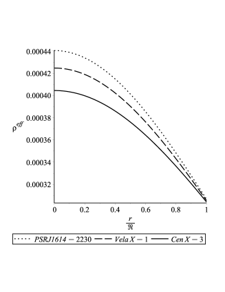
Figure 1: Variation of the effective density w.r.t. the fractional radial coordinate $r/\Re$ for different strange star candidates where $\Re$ is the radius of the corresponding star shown in Table LABEL:Table1. This explanation will be followed for all the other figures.

The effective radial pressure ($p^{eff}_{r}$) and the effective tangential pressure ($p^{eff}_{t}$), related to Eqs. (20) and (21), have been shown graphically in Fig. 2. These figures clearly indicate that both $p^{eff}_{r}$ and $p^{eff}_{t}$ are maximum at the origin ($r=0$) as in the case of the density profile and decrease gradually towards the surface. The effective radial pressure vanishes at the surface ($r={\Re}$) from where we can verify the size of our investigated stars.

In this model, anisotropy ($\Delta$) can be defined as Eq. (22). Hossein et al. [57] explained that for $\Delta>0$, i.e., $p_{t}>p_{r}$, direction of the anisotropy will be outward and for $\Delta<0$, i.e., $p_{t}<p_{r}$, anisotropy will be inward. The variation of the anisotropic stress $\Delta$ ($=p^{eff}_{t}-p^{eff}_{r}$) has been displayed in Fig. 3. This figure clearly shows the zero anisotropy at the centre of the star and then nonlinearly increasing nature throughout the stellar body. Finally, anisotropy reaches it’s maximum value at the surface which has been demanded as the inherent nature by Deb et al. [74] for ultra-dense star. Following Gokhroo and Mehra [75] we can exhibit that the positive anisotropy leads our model to achieve a stable configuration.

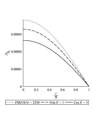
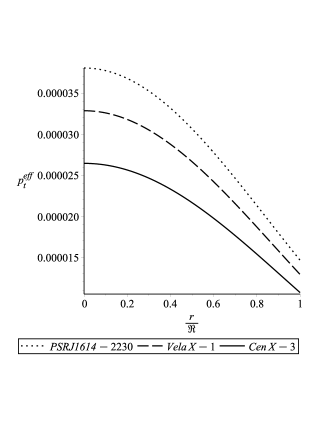
Figure 2: Variation of the effective radial pressure (left panel), effective tangential pressure (right panel) w.r.t. the fractional radial coordinate $r/\Re$ for different strange star candidates.

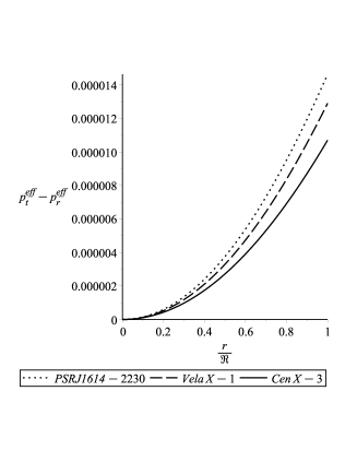
Figure 3: Variation of the anisotropic stress w.r.t. the fractional radial coordinate $r/\Re$ for different strange star candidates.

6.2 Conservation equation

The conservation equation, i.e., Tolman-Oppenheimer-Volkoff (TOV) equation has been checked to study about the stability of our model. For an anisotropic star under equilibrium, form of generalized TOV equation can be expressed as

$$\qquad-\frac{(\rho+p_{r})\nu^{\prime}}{2}-\frac{dp_{r}}{dr}+\frac{\chi}{(8\pi+2\chi)}\left[\frac{d}{dr}(\frac{p_{r}+2p_{t}}{3})-\frac{d\rho}{dr}\right]+\frac{2}{r}(p_{t}-p_{r})=0.$$ (34)

In Eq. (34), there are four different forces, viz., the gravitational $(F_{g})$, hydrostatic $(F_{h})$, anisotropic stress $(F_{a})$ and force due to modified gravity $(F_{mg})$ so that

$$F_{g}+F_{h}+F_{a}+F_{mg}=0,$$ (35)

with

$$\qquad F_{g}=-\frac{Bre^{-Ar^{2}}(A+B)}{\chi+4\pi},$$ (36)

$$\qquad F_{h}=\frac{1}{2}\frac{Are^{-Ar^{2}}(A+B)}{\chi+4\pi},$$ (37)

$$\qquad F_{a}=\frac{e^{-Ar^{2}}}{2r(12\pi+5\chi)(\chi+4\pi)}\left[3(2B^{2}r^{2}-2ABr^{2}-A+5B)\chi\right.$$

$$\qquad\left.-24\pi(A-B)(Br^{2}+3/2)\right]+\frac{6B_{g}(3\chi+4\pi)}{r(12\pi+3\chi)},$$

$$\qquad F_{mg}=\frac{(-\chi)}{(4\pi+\chi)}\left[\frac{2}{3}\frac{Are^{-Ar^{2}}(A+B)}{\chi+4\pi}+\frac{Br(B-A)e^{-Ar^{2}}}{5\chi+12\pi}-\right.$$

$$\qquad\left.\frac{\left(3Br^{2}(B-A)(\chi+2\pi)+\chi(A+10B)-6\pi(A-2B)\right)Are^{-Ar^{2}}}{3(\chi+4\pi)(5\chi+12\pi)}\right].$$ (39)

In Fig. 4, we have plotted the variation of different forces w.r.t. the radial parameter $(r)$ for different strange stars. The plots clearly indicate that the combined effect of anisotropic force and hydrostatic force balances the effect of gravitational force and modified gravity force, and our considered strange star model achieves an stable equilibrium condition under TOV stability criteria.

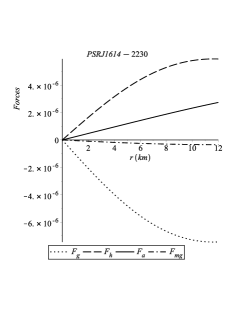
Figure 4: Variation of different forces w.r.t. the fractional radial coordinate $r/\Re$ for different strange star candidates.

6.3 Energy conditions

From general relativity, the energy-momentum tensor $\mathcal{T}_{\mu\nu}$ describes the distribution of momentum, mass and stress due to the presence of matter as well as any non-gravitational fields. The Einstein field equations, however, not directly concern about the admissible non-gravitational fields or state of matter in the spacetime model. Basically in GR the energy conditions permit different non-gravitational fields and all states of matter and also justify the physically acceptable solutions.

For a fluid sphere, composed of anisotropic strange matter, some inequality conditions like Null Energy Conditions (NEC), Strong Energy Conditions (SEC), Weak Energy Conditions (WEC) and Dominating Energy Conditions (DEC) have to hold simultaneously throughout the star, to get a stable model. These conditions are given below:

$$NEC : \rho^{eff}\geq 0,$$ (40)

$$WEC : \rho^{eff}+p_{r}^{eff}\geq 0,\rho^{eff}+p_{t}^{eff}\geq 0,$$ (41)

$$SEC : \rho^{eff}+p_{r}^{eff}+2p_{t}^{eff}\geq 0,$$ (42)

$$DEC : \rho^{eff}-|p_{r}^{eff}|\geq 0,\rho^{eff}-|p_{t}^{eff}|\geq 0.$$ (43)

At the centre ($r=0$), above energy conditions give some bounds for the model parameter $A$ and $B$. NEC, WEC, SEC, DEC demands $A>0$ , $B>0$, $(A-B)>0$ to be satisfied. Set of values shown in Table $2$ prove that our proposed strange star model successfully satisfies the energy conditions, shown in Fig. 5.

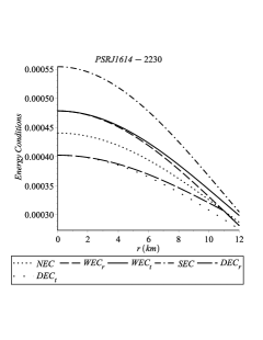
Figure 5: Variation of the different energy conditions w.r.t. the fractional radial coordinate $r/\Re$ for different strange star candidates.

However, several matter distributions are there which mathematically violate SEC. Hawking [76] argued that SEC is not valid for any scalar field containing a positive potential and for any cosmological inflationary process.

6.4 Herrera’s cracking condition

The concept of cracking (breaking) appears when the equilibrium configuration of a stellar system has been perturbed, as a result the sign of the total radial forces are different in different regions of the stellar configuration. This cracking in the stellar system arises either from the anistropy of the fluid distribution or due to the emission of incoherent radiation where the condition for the acceptability of anisotropic matter distribution is $\frac{\partial p_{r}}{\partial\rho}<1$ and $\frac{\partial p_{t}}{\partial\rho}<1$, i.e., the square of sound speed $v_{rs}^{2}<1$ and $v_{ts}^{2}<1$. With the assist of this Herrera’s cracking concept [72], we can examine the stability of our proposed model. For a physically acceptable fluid distribution, the causality condition demands the square of sound speed to follow $0\leq v^{2}_{ts}\leq 1$ and $0\leq v^{2}_{rs}\leq 1$. According to Herrera [72], the region where radial sound speed $(v_{rs})$ dominates the tangential sound speed $(v_{ts})$, is potentially stable. Also for stable matter distribution, Herrera [72] and Andréasson [77] claim the condition to be imposed is $|v^{2}_{rs}-v^{2}_{ts}|\leq 1$. This condition signifies ‘no cracking’, i.e., the region must be potentially stable.

In our model we get the parameters as follows:

$$\qquad v^{2}_{rs}=\frac{dp^{eff}_{r}}{d\rho^{eff}}=\frac{4B\chi(A-B)+\chi A(-4ABr^{2}+B^{2}r^{2}-7A+5B)+12A\pi(A+B)}{[4B\chi(A^{2}r^{2}-ABr^{2}+B)+36A^{2}\pi+27A^{2}\chi+36AB\pi+11AB\chi]},$$ (44)

$$\qquad v^{2}_{ts}=\frac{dp^{eff}_{t}}{d\rho^{eff}}=\frac{-2({A}^{2}B{r}^{2}-A{B}^{2}{r}^{2}+{A}^{2}-3AB+{B}^{2})(12\pi+5\chi)}{(4A^{2}B\chi r^{2}-4AB^{2}\chi r^{2}+36A^{2}\pi+27A^{2}\chi+36AB\pi+11AB\chi+4B^{2}\chi)}.$$ (45)

In GR, for any model following the MIT bag EOS, the value of the square of radial sound speed ($v_{rs}^{2}$) is a constant ($1/3$). But, due to the coupling parameter ($\chi$) in the modified gravity, $v_{rs}^{2}$ becomes as Eq. (44), where $\chi=0$ gives back the constant result as can be achieved in GR.

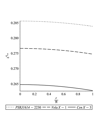
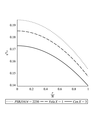
Figure 6: Variation of $v^{2}_{rs}$ (left panel), $v^{2}_{ts}$ (right panel) w.r.t. the fractional radial coordinate $r/\Re$ for different strange star candidates.

Graphical representation for causality conditions and Herrera’s cracking condition [72] have been shown in Fig. 6 and Fig. 7 respectively. From Fig. 6, it is clear that both $v^{2}_{rs}$ and $v^{2}_{ts}$ are less than 1, i.e., our model is consistent with Herrera’s cracking concept and Fig. 7 also shows potential stability throughout the stars.

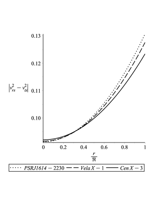
Figure 7: Variation of $|v^{2}_{rs}-v^{2}_{ts}|$ w.r.t. the fractional radial coordinate $r/\Re$ for different strange star candidates.

6.5 Effective mass and compactification factor

For a spherically symmetric, static strange star made of perfect anisotropic fluid, Buchdahl [78] established that there is an upper limit for the ratio of allowed maximum mass and radius $(\Re)$, i.e., $\frac{2M}{\Re}<\frac{8}{9}$. In our proposed model, the gravitational effective mass takes the following form

$$M^{eff}=\int_{0}^{\Re}4\pi r^{2}\rho^{eff}dr=\int_{0}^{\Re}4\pi r^{2}\left[\rho+\frac{\chi}{4\pi}\left(2\rho-\frac{p_{r}+2p_{t}}{3}\right)\right]dr$$

$$=m+\int_{0}^{\Re}r^{2}\chi\left(2\rho-\frac{p_{r}+2p_{t}}{3}\right)dr,$$ (46)

where $m=4\pi\int_{0}^{\Re}r^{2}\rho dr$ is mass function for the distribution of strange quark matter and the remaining part $\int_{0}^{\Re}r^{2}\chi\left(2\rho-\frac{p_{r}+2p_{t}}{3}\right)dr=m_{mg}$ is another mass distribution which has been generated due to the modified gravity. For $\chi=0$ Eq. (46) leads to the GR solution, i.e. $M^{eff}=m$.

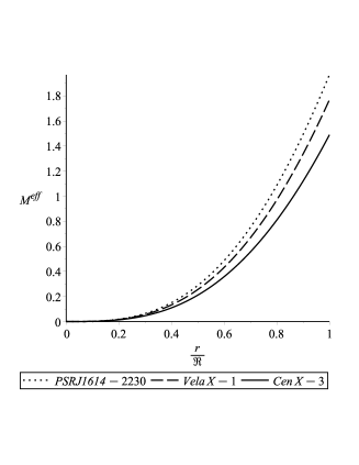
Figure 8: Variation of the effective mass w.r.t. the fractional radial coordinate $r/\Re$ for different strange star candidates.

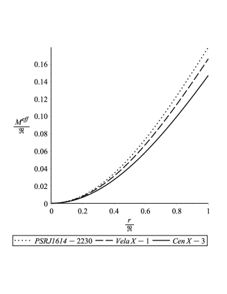
Figure 9: Variation of the compactness w.r.t. the fractional radial coordinate $r/\Re$ for different strange star candidates.

The compactification factor $u(r)$ can be defined as the ratio of the effective mass $(M^{eff})$ and radius $(\Re)$, which is given below

$$\qquad u(r)=\frac{M^{eff}(r)}{\Re}=\frac{1}{\Re}[m+\int_{0}^{\Re}r^{2}\chi\left(2\rho-\frac{p_{r}+2p_{t}}{3}\right)dr].$$ (47)

The variation of effective mass and compactification factor w.r.t. to $\frac{r}{\Re}$ have been shown graphically in Figs. 8 and 9 respectively, where both increase with increasing radii.

6.6 Surface redshift

The surface redshift is defined as

$$Z_{s}=\frac{1}{\sqrt{1-2u}}-1.$$ (48)

Barraco and Hamity [79] showed that for an isotropic star, $Z_{s}\leq 2$ when the cosmological constant is absent. Later, Böhmer and Harko  [80] proved that surface redshift may be much higher ($Z_{s}\leq 5$) for an anisotropic star when the cosmological constant is present. Eventually, this restriction get modified, and calculations show that $Z_{s}=5.211$  [81] is the maximum acceptable limit. In the current study, we have calculated the value for maximum surface redshift for different strange stars and get $Z_{s}\leq 1$ [ LABEL:Table4] in every case.

6.7 Equation of State (EOS)

According to our proposed model, we can represent radial ($\omega_{r}$) and tangential ($\omega_{t}$) EOS as follows

$$\qquad\omega_{r}=\frac{p^{eff}_{r}}{\rho^{eff}}=\frac{\left[\alpha\chi+12\pi(A+B)\right]{e^{-A{r}^{2}}}-12(4\pi+3\chi)B_{g}(\chi+4\pi)}{\left[\beta\chi+36\pi(A+B)\right]{e^{-A{r}^{2}}}+12(4\pi+3\chi)B_{g}(\chi+4\pi)},$$ (49)

$$\qquad\omega_{t}=\frac{p^{eff}_{t}}{\rho^{eff}}=\frac{-2(AB{r}^{2}-{B}^{2}{r}^{2}+A-2B){e^{-Ar^{2}}}(12\pi+5\chi)}{[\beta\chi+36\pi(A+B)]e^{-Ar^{2}}+12(4\pi+3\chi)B_{g}(\chi+4\pi)},$$ (50)

where $\alpha=(-4AB{r}^{2}+4{B}^{2}{r}^{2}-7A+5B)$, $\beta=(4ABr^{2}-4B^{2}r^{2}+27A+15B)$. We have plotted EOS parameter $(\omega)$ w.r.t. the fractional radial coordinate $\frac{r}{\Re}$, for both EOS $\omega_{r}$ and $\omega_{t}$, shown in Fig. 10. The figures clearly show that throughout the fluid sphere, $\omega_{r}$ and $\omega_{t}$ are positive and they lie in $0<\omega<1$, which establish the non-exotic nature of strange quintessence star.

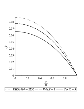
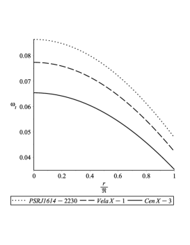
Figure 10: Variation of the EOS parameter $w_{r}$ (left panel) and $w_{t}$ (right panel) w.r.t. the fractional radial coordinate $r/\Re$ for different strange star candidates.

6.8 Adiabatic index

The adiabatic index $\Gamma$ can be described as the ratio of two specific heat [82] and for a given density profile, $\Gamma$ characterizes the stiffness of that EOS. Chandrasekhar [83] introduced the idea of the dynamical stability of the stellar model against an infinitesimal radial adiabatic perturbation. Later on this stability condition was developed and used at astrophysical level by several scientists [84, 85, 86, 87, 88]. The stability condition demands that the adiabatic index $\Gamma>\frac{4}{3}$. For the anisotropic relativistic sphere the radial and transverse adiabatic index as $\Gamma_{r}$ and $\Gamma_{t}$ respectively, can be expressed as

$$\Gamma_{r} = \frac{\rho^{eff}+p_{r}^{eff}}{p_{r}^{eff}}\left[\frac{dp_{r}^{eff}}{d\rho^{eff}}\right],$$ (51)

$$\Gamma_{t} = \frac{\rho^{eff}+p_{t}^{eff}}{p_{t}^{eff}}\left[\frac{dp_{t}^{eff}}{d\rho^{eff}}\right].$$ (52)

In our model, using above relations, we get the following equations

$$\qquad\Gamma_{r}=\frac{(12\pi+5\chi)\gamma\left[\left((Br^{2}+\frac{7}{4})A^{2}-(B^{2}r^{2}+\frac{9B}{4})A+B^{2}\right)\chi-3A\pi\gamma\right]\phi}{[\left(\alpha\chi-3\pi\gamma\right)\phi+6\beta]\left[\left(\xi A^{2}+(-B^{2}r^{2}+\frac{11B}{4})A+B^{2}\right)\chi+9A\pi\gamma\right]},$$ (53)

$$\qquad\Gamma_{t}=\frac{\delta\left[\left(-r^{2}B^{2}\kappa+B\left(Ar^{2}\kappa-\frac{7\pi}{2}-\frac{35\chi}{24}\right)-A(\frac{\pi}{2}+\frac{17\chi}{24})\right)\phi-\beta\right]}{\theta\phi\left[B^{2}\chi(1-Ar^{2})+A(A\chi r^{2}+9\pi+\frac{11\chi}{4})B+9A^{2}(\pi+\frac{3\chi}{4})\right]},$$ (54)

where, $\alpha=(ABr^{2}-B^{2}r^{2}+\frac{7A}{4}-\frac{5B}{4})$, $\beta=\frac{B_{g}}{2}(4\pi+3\chi)(\chi+4\pi)$, $\gamma=(A+B)$, $\delta=-6[(1-Ar^{2})B^{2}+(Ar^{2}-3)AB+A^{2}]$, $\phi=e^{-Ar^{2}}$, $\xi=(Br^{2}+\frac{27}{4})$, $\kappa=(\frac{\chi}{4}+\pi)$ and $\theta=(ABr^{2}-B^{2}r^{2}+A-2B)$.

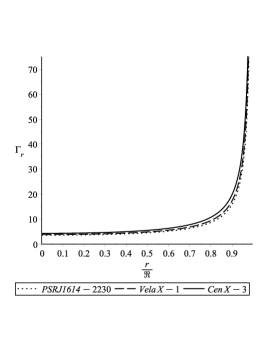
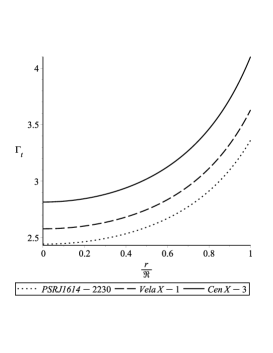
Figure 11: Variation of the adiabatic index $\Gamma_{r}$ (left panel) and $\Gamma_{t}$ (right panel) w.r.t. the fractional radial coordinate $r/\Re$ for different strange star candidates.

It can be shown analytically that both the adiabatic indices $(\Gamma_{r},~{}\Gamma_{t})>\frac{4}{3}$ throughout the interior of the strange star and thus satisfy the stability condition. The graphical representations (Fig. 11) also establish the stability of our proposed model.

6.9 Harrison-Zel^′dovich-Novikov static stability criteria

In 1964, Chandrasekhar [89] and in 1965 Harrison et al.  [90] calculate the eigen-frequencies for all the fundamental modes. Later, Zel^′dovich and Novikov [91] make the calculations more simpler following Harrison et al. [90]. For that purpose, they assumed that adiabatic index of a slowly deformed matter is comparable with that of a pulsating star. From their assumption, nature of mass will be increasing w.r.t the central density (i.e. $\frac{dM}{d\rho_{c}}>0$) for a stable configuration. Model will be unstable if $\frac{dM}{d\rho_{c}}<0$.

In this model, mass can be expressed in terms of the central density ($\rho_{c}$) as follows

$$\qquad M(\rho_{c})=\frac{R^{3}[16\pi(12\pi\beta-12\pi\rho_{c}+12\beta\chi-5\chi\rho_{c})+36\chi^{2}\beta+36A\pi+27A\chi]}{[32\pi R^{2}(12\pi\beta-12\pi\rho_{c}+12\beta\chi-5\chi\rho_{c})+18R^{2}(4\beta\chi^{2}+4A\pi+3A\chi)-36\pi-15\chi]}.$$ (55)

Differentiating Eq. (55) w.r.t. $\rho_{c}$ we get

$$\qquad\frac{dM}{d\rho_{c}}=\frac{48R^{3}\pi(12\pi+5\chi)^{2}}{[32\pi R^{2}(12\pi\beta-12\pi\rho_{c}+12\beta\chi-5\chi\rho_{c})+18R^{2}(4\beta\chi^{2}+4A\pi+3A\chi)-36\pi-15\chi]^{2}}.$$ (56)

From Eq. (56), it is very clear that $\frac{dM}{d\rho_{c}}$ is always positive inside the star and Fig. 12 also shows the positive value for $\frac{dM}{d\rho_{c}}$ throughout the stellar structure. So, our model fulfils the Harrison-Zel^′dovich-Novikov condition and further confirms the stability [92, 93].

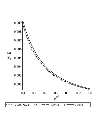
Figure 12: Variation of $\frac{dM}{d\rho_{c}}$ w.r.t. $\rho_{c}$ for different strange star candidates.

7 Discussions and conclusions

In this paper, we have explored strange quark star in $f(R,T)$ gravity using the KB [1] metric functions, where we assume the MIT bag model as the EOS for strange quark matter distribution. Since, the matter distribution is assumed to be anisotropic in nature, the system is not at all over determined due to inclusion of the EOS. With the help of the KB metric and the MIT bag model as EOS, we have investigated here various interesting physical features and also represented graphically, the variation of different physical parameters w.r.t. the fractional radial coordinate $r/\Re$.

However, the specific major findings of the present investigation can be categorized as follows:

1. From our study we can predict the existence of stable strange stars in the range of lower value of $B_{g}$ $(40-45)~{}Mev/fm^{3}$ whereas earlier works assumed [64, 94] or obtained [55, 95] higher values of $B_{g}$ for the construction of strange stellar models in both GR [55, 95] and modified theories [64, 94]. Our investigation, therefore, clearly indicates that $f(R,T)$ gravity effectively reduces $B_{g}$. Here the matter-geometry coupling constant $\chi$ plays an important role for this reduction. Setting $\chi=0$ in the results of our study, one can get the higher values of $B_{g}$ in the range $(55-75)~{}Mev/fm^{3}$ which is till now the proposed range [2, 3, 96] for stable strange quark matter distribution under GR. However, experimental results from RHIC and CERN-SPS, show the possibility of wide range of value for bag constant in case of density dependent bag model [97]. In Table LABEL:Table2, we have provided the calculated bag value from our model. At the same time, incorporating $\chi=0$ in Eq. (33) we have again calculated the bag value, which actually signifies $B_{g}$ in the frame of GR. In the second case, we get $B_{g}$ in the range $(57-60)~{}Mev/fm^{3}$, shown in Table LABEL:Table3 which strongly supports the stability criteria [2, 3].

2. Following the earlier works [55, 95, 64, 94], we have checked the stability issue of strange stars through the studies of Herrera’s cracking conditions, energy conditions, Buchdahl limit, TOV equation, EOS parameter and adiabatic index. Variations of all these parameters w.r.t. the fractional radial coordinate $r/\Re$ clearly indicate the stability of our model and physical acceptability for the construction of stable strange star under $f(R,T)$ gravity with KB spacetime. In addition to above, we have also checked the criteria of Harrison-Zel^′dovich-Novikov for static stability which is well satisfied. This is very crucial point to note that none of the earlier works [55, 95, 64, 94] satisfies all the stability criteria at a time as our study does effectively.

3. The present study can be claimed as a continuation of the earlier works [55, 95, 64, 94] which provides more promising results by fine tuning of various model parameters.

Now we would like to summarize all the general features of the present study as follows:

(i) Density and Pressure: In our present investigation the effective density ($\rho^{eff}$), effective radial pressure ($p^{eff}_{r}$), effective tangential pressure ($p^{eff}_{t}$) have been shown graphically in Figs. 1 and 2. Here $\rho^{eff}$, $p^{eff}_{r}$, $p^{eff}_{t}$ all are maximum at the centre with positive signature and decrease while approach to the surface. We can measure the effective surface density and verify the radius of the star from the cut on $r$-axis. These high values of the central as well as the effective surface density clearly emphasize the fact that our chosen stellar candidates are highly compact, and thus actually represent themselves as strange quark star candidates [98, 99, 100]. On the other hand, plot of the anisotropic stress (Fig. 3) demonstates the physical stability of our model.

(ii) TOV equation: In our model the plots (Fig. 4) for the generalized force condition (TOV equation), show that our stellar model remains in static equilibrium under the combined effect of four different forces, viz. hydrostatic force ($F_{h}$), gravitational force ($F_{g}$), anisotropic force ($F_{a}$) and the additional modified gravity force ($F_{mg}$). Here, the newly added force, represented as the modified gravity force ($F_{mg}$) implies the coupling between matter and geometry.

(iii) Energy conditions: In our study, we have graphically represented (Fig. 5) that the variation of different energy conditions, namely WEC, NEC, SEC and DEC satisfies for the prescribed anisotropic fluid distribution consisting of strange quark matter.

(iv) Stabilty of model: Following Herrera’s [72] cracking condition, $v^{2}_{rs}$ and $v^{2}_{ts}$ should lie between the limit 0 and 1. Figs. 6 and  7 clearly show that $v^{2}_{rs}$, $v^{2}_{ts}$ , $|v^{2}_{rs}-v^{2}_{ts}|$ remain in this limit, within the fluid distribution. So from cracking concept and causality condition  [72, 77], our model is physically reasonable as well as potentially stable. In the left panel of Fig. 6, $v^{2}_{rs}$ is not a constant, rather it shows non-linearly decreasing nature with the increasing radii and numerical value remains slightly smaller than $1/3$ for all the stars. Here, putting $\chi=0$ in Eq. (44), we get back $v^{2}_{rs}=1/3$ which signifies the constant value for radial sound speed in GR.

Variation of the EOS parameter for both the radial and tangential cases, have been displayed in Fig. 10. Within the fluid distribution, value of the EOS parameter is always positive and less than 1, which is another evidence for the stability of our proposed model. On the other hand, variations of adiabatic indices, plotted in Fig. 11, evidently show that both $\Gamma_{r}$ and $\Gamma_{t}$ are greater than $4/3$ throughout the stellar system, obeying Bondi’s [84] stable configuration criteria.

In this model, static stability criteria privided by Harrison, Zel^′dovich and Novikov  [90, 91] is also satisfied (Eq. (56)) for different strange stars. Fig. 12 also shows that $\frac{dM}{d\rho_{c}}>0$ always within the stellar structure and reduces for higher radial value.

(v) Buchdahl Condition: The effective mass function up to the surface (i.e. the radius $r$) has been shown in Fig. 8. This figure shows that $M_{eff}(r)\rightarrow 0$ for $r\rightarrow 0$ which emphasizes on the regularity of $M_{eff}(r)$ at $r=0$, i.e., at the centre. In case of the spherically symmetric, static and perfect fluid distribution, Buchdahl [78] established a condition for the mass and radius ratio, i.e., $\frac{2M}{\Re}\leq\frac{8}{9}$. In our study, we consider three strange star candidates (Table 1), for which Buchdahl condition [78] is satisfied. Here $\frac{2M}{\Re}$ ratio exists in the range $(0.29-0.35)$.

(vi) Compactness and surface redshift: We have studied three different strange star candidates, namely $PSR~{}J~{}1614-2230$, $Vela~{}X-1$, $Cen~{}X-3$ whose mass and radius are provided in Table 1 [73]. Variation of the compactification factor w.r.t. $r/{\Re}$ has been presented in Fig. 9 where the revealed features are highly reasonable for strange stars. Here we find high surface redshift $(0.2-0.25)$ which establishes that our model stars represent some possible candidates for strange stars which are stable in their configuration.

In connection to stability, there are several research works available on modified gravity on strange stars which provide stability though the problem of singularity arises at the centre. On the other hand, few works do not satisfy all the stability criteria, energy conditions, Buchdahl limit [78] one at a time. However, in the present study using the KB metric and the MIT bag model in modified gravity (i.e. $f(R,T)$), our proposed model is completely free from any singularity and satisfies all the stability criteria.

As a final concluding remark, the present study on stellar model is nothing but the representative of highly dense stars formed with strange quark matter and perfectly suitable for investigating various features of strange stars. Besides that, most fascinating fact is the effect of modified gravity on the bag constant $B_{g}$ as shown in Table LABEL:Table3. Due to the coupling between matter and geometry, there arises a coupling term $\chi$ which effectively reduces the bag value as well as the square of radial sound speed, which generally remains constant ($1/3$) in GR. In every case, putting $\chi=0$, one can retrieve the results which perfectly match the GR results.

References

- [1] K.D. Krori, J. Barua, J. Phys. A: Math. Gen. 8 (1975) 508.
- [2] E. Farhi, R.L. Jaffe, Phys. Rev. D 30 (1984) 2379.
- [3] C. Alcock, E. Farhi, A. Olinto, Astrophys. J. 310 (1986) 216.
- [4] A. Hewish, S.J. Bell, J.D.H. Pilkington, P.F. Scott, R.A. Collins, Nature 217 (1968) 709.
- [5] P.B. Demorest, T. Pennucci, S.M. Ransom, M.S.E. Roberts, J.W.T. Hessels, Nature 467 (2010) 1081.
- [6] M. Brilenkov, M. Eingorn, L. Jenkovszky, A. Zhuk, JCAP 08 (2013) 002.
- [7] S.D. Maharaj, J.M. Sunzu, S. Ray, Eur. Phys. J. Plus. 129 (2014) 3.
- [8] L. Paulucci, J.E. Horvath, Phys. Lett. B 733 (2014) 164.
- [9] N.R. Panda, K.K. Mohanta, P.K. Sahu, J. Physics: Conf. Ser. 599 (2015) 012036.
- [10] A.A. Isayev, Phys. Rev. C 91 (2015) 015208.
- [11] G. Abbas, S. Qaisar, A. Jawad, Astrophys. Space Sci. 359 (2015) 57.
- [12] J.D.V. Arbañil, M. Malheiro, JCAP 11 (2016) 012.
- [13] G. Lugones, J.D.V. Arbañil, Phys. Rev. D 95 (2017) 064022.
- [14] A.G. Riess et al., Astron. J. 116 (1998) 1009.
- [15] S. Perlmutter et al., Astrophys. J. 517 (1999) 565.
- [16] P. de Bernardis et al., Nature 404 (2000) 955.
- [17] S. Hanany et al., Astrophys. J. 545 (2000) L5.
- [18] P.J.E. Peebles, B. Ratra, Rev. Mod. Phys. 75 (2003) 559.
- [19] T. Padmanabhan, Phys. Repts. 380 (2003) 235.
- [20] T. Clifton, P.G. Ferreira, A. Padilla, C. Skordis, Phys. Rep. 513 (2012) 1.
- [21] B. Jain, A. Taylor, Phys. Rev. Lett. 91 (2003) 141302.
- [22] M. Tegmark et al., Phys. Rev. D 69 (2004) 103501.
- [23] D.J. Eisentein et al., Astrophys. J. 633 (2005) 560.
- [24] D.N. Spergel et al., Astrophys. J. Suppl. 170 (2007) 377.
- [25] E.J. Copeland, M. Sami, S. Tsujikawa, Int. J. Mod. Phys. D 15 (2006) 1753.
- [26] S. Nojiri, S.D. Odintsov, Int. J. Geom. Meth. Mod. Phys. 4 (2007) 115.
- [27] S. Tsujikawa, Lect. Not. Phys. 800 (2010) 99.
- [28] S. Nojiri, S.D. Odintsov, Phys. Rev. D 68 (2003) 123512.
- [29] S.M. Carroll, V. Duvvuri, M. Trodden, M.S. Turner, Phys. Rev. D 70 (2004) 042528.
- [30] A.A. Starobinsky, J. Exp. Theo. Phys. Lett. 86 (2007) 157.
- [31] K. Bamba, S. Nojiri, S.D. Odintsov, J. Cosmol. Astropart. Phys. 0810 (2008) 045.
- [32] M.R. Setare, M. Jamil, Gen. Relativ. Gravit. 43 (2011) 293.
- [33] M. Jamil, F.M. Mahomed, D. Momeni, Phys. Lett. B 702 (2011) 315.
- [34] I. Hussain, M. Jamil, F.M. Mahomed, Astrophys Space Sci. 337 (2012) 373.
- [35] G. Abbas, S. Nazeer, M.A. Meraj, Astrophys. Space Sci. 354 (2014) 449.
- [36] G. Abbas, A. Kanwal, M. Zubair, Astrophys. Space Sci. 357 (2015) 109.
- [37] G. Abbas et al., Astrophys. Space Sci. 357 (2015) 158.
- [38] G. Abbas, S. Qaisar, M.A. Meraj, Astrophys. Space Sci. 357 (2015) 156.
- [39] M. Zubair, G. Abbas, I. Noureen, Astrophys. Space Sci. 361 (2016) 8.
- [40] B.T. Harko, F.S.N. Lobo, S. Nojiri, S.D. Odintsov, Phys. Rev. D 84 (2011) 024020.
- [41] P.H.R.S. Moraes, Astrophys. Space Sci. 352 (2014) 273.
- [42] P.H.R.S. Moraes, Eur. Phys. J. C 75 (2015) 168.
- [43] P.H.R.S. Moraes, G. Ribeiro, R.A.C. Correa, Astrophys. Space Sci. 361 (2016) 227.
- [44] P.H.R.S. Moraes, R.A.C. Correa, Astrophys. Space Sci. 361 (2016) 91.
- [45] P.H.R.S. Moraes, J.R.L. Santos, Eur. Phys. J. C 76 (2016) 60.
- [46] P.H.R.S. Moraes, Int. J. Theor. Phys. 55 (2016) 1307.
- [47] R.A.C. Correa, P.H.R.S. Moraes, Eur. Phys. J. C 76 100 (2016).
- [48] M. Sharif, M. Zubair, JCAP 03, (2012) 028.
- [49] D. Momeni, P.H.R.S. Moraes, R. Myrzakulov, Astrophys. Space Sci. 361 (2016) 228.
- [50] M.F. Shamir, Eur. Phys. J. C 75 (2015) 354.
- [51] I. Noureen, M. Zubair, A.A. Bhatti, G. Abbas, Eur. Phys. J. C 75 (2015) 323.
- [52] P.H.R.S. Moraes, J.D.V. Arbañil, M. Malheiro, JCAP 06 (2016) 005.
- [53] M. Alves, P. Moraes, J. de Araujo, M. Malheiro, Phys. Rev. D 94 (2016) 024032.
- [54] A. Das, S. Ghosh, B.K. Guha, S. Das, F. Rahaman, S. Ray, Phys. Rev. D 95 (2017) 124011.
- [55] F. Rahaman, R. Sharma, S. Ray, R. Maulick, I. Karar, Eur. Phys. J. C 72 (2012) 2071.
- [56] M. Kalam et al., Eur. Phys. J. C 72, 2248 (2012).
- [57] Sk.M. Hossein, F. Rahaman, J. Naskar, M. Kalam, S. Ray, Int. J. Mod. Phys. D 21 (2012) 1250088.
- [58] M. Kalam, F. Rahaman, Sk.M. Hossein, S. Ray, Eur. Phys. J. C 73 (2013) 2409.
- [59] P. Bhar, Astrophys. Space Sci. 356 (2015) 309.
- [60] P. Bhar, Astrophys. Space Sci. 356 (2015) 365.
- [61] P. Bhar, Astrophys. Space Sci. 357 (2015) 46.
- [62] G. Abbas, M. Zubair, G. Mustafa, Astrophys. Space Sci. 358 (2015) 26.
- [63] D. Momeni, G. Abbas, S. Qaisar, Z. Zaz, R. Myrzakulov, arXiv:1611.03727 [gr-qc].
- [64] D. Deb, F. Rahaman, S. Ray, B.K. Guha. J. Cosmol. Astropart. Phys. 03 (2018) 044.
- [65] O.J. Barrientos, G.F. Rubilar, Phys. Rev. D 90 (2014) 028501.
- [66] D.R.K. Reddy, R.S. Kumar, Astrophys. Space Sci. 344 (2013) 253.
- [67] P.H.R.S. Moraes, Astrophys. Space Sci. 352 (2014) 273.
- [68] V. Singh, C.P. Singh, Astrophys. Space Sci. 356 (2015) 153.
- [69] P.H.R.S. Moraes, Eur. Phys. J. C 75 (2015) 168.
- [70] P.H.R.S. Moraes, Int. J. Theor. Phys. 55 (2016) 1307.
- [71] P. Kumar, C.P. Singh, Astrophys. Space Sci. 357 (2015) 120.
- [72] L. Herrera, Phys. Lett. A 165 (1992) 206.
- [73] D. Deb, S.R. Chowdhury, B.K. Guha, S. Ray, arXiv:1611.02253.
- [74] D. Deb, S. Roy Chowdhury, S. Ray, F. Rahaman, B.K. Guha, Ann. Phys. (Amsterdam) 387 (2017) 239.
- [75] M.K. Gokhroo, A.L. Mehra, Gen. Relativ. Gravit. 26 (1994) 75.
- [76] S. Hawking, G.F.R. Ellis, The Large Scale Structure of Space-Time. Cambridge University Press, Cambridge (1973).
- [77] H. Andréasson, Commun. Math. Phys. 288 (2009) 715.
- [78] H.A. Buchdahl, Phys. Rev. 116 (1959) 1027.
- [79] D.E. Barraco, V.H. Hamity, Phys. Rev. D. 65 (2002) 124028.
- [80] C.G. Böhmer, T. Harko, Classical Quantum Gravity 23 (2006) 6479.
- [81] B.V. Ivanov, Phys. Rev. D 65 (2002) 104011.
- [82] W. Hillebrandt, K.O. Steinmetz, Astron. Astrophys. 53 (1976) 283.
- [83] S. Chandrasekhar, Astrophys. J. 140 (1964) 417.
- [84] H. Bondi, Proc. R. Soc. Lond. Series A, Math. Phys. Sci. 281 (1964) 39.
- [85] J.M. Bardeen, K.S. Thorne, D.W. Meltzer, Astrophys. J. 145 (1966) 505.
- [86] R.M. Wald, General Relativity (Chicago Press, Chicago and London, p. 127 (1984).
- [87] H. Knutsen, MNRAS 232, (1988) 163.
- [88] M.K. Mak, T. Harko, Eur. Phys. J. C 73, (2013) 2585.
- [89] S. Chandrasekhar, Phys. Rev. Lett. 12 (1964) 114.
- [90] B.K. Harrison, K.S. Thorne, M. Wakano, J.A. Wheeler, Gravitational Theory and Gravitational Collapse (Chicago: University of Chicago Press) (1965).
- [91] Ya.B. Zel′dovich, I.D. Novikov, Relativistic Astrophysics Vol. 1: Stars and Relativity (Chicago: University of Chicago Press) (1971).
- [92] D. Shee, F. Rahaman, B.K. Gupta, S. Ray, Astrophys. Space Sci. 361 (2016) 167.
- [93] P. Bhar, K.N. Singh, F. Rahaman, N. Pant, S. Banerjee, Int. J. Mod. Phys. D 26 (2017) 15.
- [94] D. Deb, B. K. Guha, F. Rahaman, S. Ray, Phy. Rev. D 97, 084026 (2018).
- [95] P. Bhar, Astrophys. Space Sci. 357 (2015) 46.
- [96] F. Weber, Prog. Part. Nucl. Phys. 54 (2005) 193.
- [97] G.F. Burgio, M. Baldo, P.K. Sahu, H.-J. Schulze, Phys. Rev. C 66 (2002) 025802.
- [98] R. Ruderman, Pulsars: Structure and Dynamics, Rev. Astron. Astrophys. 10 (1972) 427.
- [99] N.K. Glendenning, Compact Stars: Nuclear Physics, Particle Physics and General Relativity, Springer, New York, pg. 468 (1997).
- [100] M. Herzog, F.K. Röpke, Phys. Rev. D 84 (2011) 083002.