Quantum metrology with quantum-chaotic sensors

Abstract

Quantum metrology promises high-precision measurements of classical parameters with far reaching implications for science and technology. So far, research has concentrated almost exclusively on quantum-enhancements in integrable systems, such as precessing spins or harmonic oscillators prepared in non-classical states. Here we show that large benefits can be drawn from rendering integrable quantum sensors chaotic, both in terms of achievable sensitivity as well as robustness to noise, while avoiding the challenge of preparing and protecting large-scale entanglement. We apply the method to spin-precession magnetometry and show in particular that the sensitivity of state-of-the-art magnetometers can be further enhanced by subjecting the spin-precession to non-linear kicks that renders the dynamics chaotic.

Introduction

Quantum-enhanced measurements (QEM) use quantum effects in order to measure physical quantities with larger precision than what is possible classically with comparable resources. QEMs are therefore expected to have large impact in many areas, such as improvement of frequency standards Huelga97 ; PhysRevLett.86.5870 ; Leibfried04 ; wasilewski2010quantum ; koschorreck2010sub , gravitational wave detection Goda08 ; aasi2013enhanced , navigation Giovannetti01 , remote sensing Allen08radar , or measurement of very small magnetic fields Taylor08 . A well known example is the use of so-called NOON states in an interferometer, where a state with $N$ photons in one arm of the interferometer and zero in the other is superposed with the opposite situation Boto00 . It was shown that the smallest phase shift that such an interferometer could measure scales as $1/N$, a large improvement over the standard $1/\sqrt{N}$ behavior that one obtains from ordinary laser light. The latter scaling is known as the standard quantum limit (SQL), and the $1/N$ scaling as the Heisenberg limit (HL). So far the SQL has been beaten only in few experiments, and only for small $N$ (see e.g. Higgins07 ; Leibfried04 ; Nagata07 ), as the required non-classical states are difficult to prepare and stabilize and are prone to decoherence.
Sensing devices used in quantum metrology so far have been based almost exclusively on integrable systems, such as precessing spins (e.g. nuclear spins, NVcenters, etc.) or harmonic oscillators (e.g. modes of an electro-magnetic field or mechanical oscillators), prepared in non-classical states (see pezze_non-classical_2016 for a recent review). The idea of the present work is to achieve enhanced measurement precision with readily accessible input states by disrupting the parameter coding by a sequence of controlled pulses that render the dynamics chaotic. At first sight this may appear a bad idea, as measuring something precisely requires well-defined, reproducible behavior, whereas classical chaos is associated with unpredictible long-term behavior. However, the extreme sensitivity to initial conditions underlying classically chaotic behavior is absent in the quantum world with its unitary dynamics in Hilbert space that preserves distances between states. In turn, quantum-chaotic dynamics can lead to exponential sensitivity with respect to parameters of the system Peres91 .
The sensitivity to changes of a parameter of quantum-chaotic systems has been studied in great detail with the technique of Loschmidt echo Gorin06review , which measures the overlap between a state propagated forward with a unitary operator and propagated backward with a slightly perturbed unitary operator. In the limit of infinitesimally small perturbation, the Loschmidt echo turns out to be directly related to the quantum Fisher information (QFI) that determines the smallest uncertainty with which a parameter can be estimated. Hence, a wealth of known results from quantum chaos can be immediately translated to study the ultimate sensitivity of quantum-chaotic sensors. In particular, linear response expressions for fidelity can be directly transfered to the exact expressions for the QFI.
Ideas of replacing entanglement creation by dynamics were proposed previously Boixo08.2 ; xiao2011chaos ; song2012quantum ; weiss2009signatures ; frowis2016detecting , but focussed on initial state preparation, or robustness of the readout macri2016loschmidt ; linnemann2016quantum , without introducing or exploiting chaotic dynamics during the parameter encoding. They are hence comparable to spin-squeezing of the input state ma2011quantum . Quantum chaos is also favorable for state tomography of random initial states with weak continuous time measurement madhok2014information ; madhok2016review , but no attempt was made to use this for precision measurements of a parameter. A recent review of other approaches to quantum-enhanced metrology that avoid initial entanglement can be found in braun2017without .
We study quantum-chaotic enhancement of sensitivity at the example of the measurement of a classical magnetic field with a spin-precession magnetometer. In these devices that count amongst the most sensitive magnetometers currently available allred2002high ; Kominis03 ; savukov2005effects ; budker2007optical ; sheng2013subfemtotesla , the magnetic field is coded in a precession frequency of atomic spins that act as the sensor. We show that the precision of the magnetic-field measurement can be substantially enhanced by non-linearly kicking the spin during the precession phase and driving it into a chaotic regime. The initial state can be chosen as an essentially classical state, in particular a state without initial entanglement. The enhancement is robust with respect to decoherence or dissipation. We demonstrate this by modeling the magnetometer on two different levels: firstly as a kicked top, a well-known system in quantum chaos to which we add dissipation through superradiant damping; and secondly with a detailed realistic model of a spin-exchange-relaxation-free atom-vapor magnetometer including all relevant decoherence mechanisms allred2002high ; appelt1998theory , to which we add non-linear kicks.

Results

Physical model of a quantum-chaotic sensor

As a sensor we consider a kicked top (KT), a well-studied quantum-chaotic system haake1987classical ; kickedtop ; haake2013quantum described by the time-dependent Hamiltonian

$${H}_{\text{KT}}(t)=\alpha J_{z}+\frac{k}{2J}J_{y}^{2}\sum_{n=-\infty}^{\infty}\tau\delta(t-n\tau)\,,$$ (1)

where $J_{i}$ ($i=x,y,z$) are components of the (pseudo-)angular momentum operator, $J\equiv j+1/2$, and we set $\hbar=1$. $J_{z}$ generates a precession of the (pseudo-)angular momentum vector about the $z$-axis with precession angle $\alpha$ which is the parameter we want to estimate. “Pseudo” refers to the fact that the physical system need not be an actual physical spin, but can be any system with $2j+1$ basis states on which the $J_{i}$ act accordingly. For a physical spin-$j$ in a magnetic field $B$ in $z$-direction, $\alpha$ is directly proportional to $B$. The $J_{y}^{2}$-term is the non-linearity, assumed to act instantaneously compared to the precession, controlled by the kicking strength $k$ and applied periodically with a period $\tau$ that leads to chaotic behavior. The system can be described stroboscopically with discrete time $t$ in units of $\tau$ (set to $\tau=1$ in the following),

$$|\psi(t)\rangle=U_{\alpha}(k)|\psi(t-1)\rangle=U^{t}_{\alpha}(k)|\psi(0)\rangle$$ (2)

with the unitary Floquet-operator

$$U_{\alpha}(k)=T\exp\left(-i\int_{t}^{t+1}\ dt^{\prime}{H}_{\text{KT}}(t^{\prime})\right)=e^{-ik\frac{J^{2}_{y}}{2J}}e^{-i\alpha J_{z}}$$ (3)

that propagates the state of the system from right after a kick to right after the next kick haake1987classical ; kickedtop ; haake2013quantum . $T$ denotes time-ordering. The total spin is conserved, and $1/J$ can be identified with an effective $\hbar$, such that the limit $j\to\infty$ corresponds to the classical limit, where $X=J_{x}/J$, $Y=J_{y}/J$, $Z=J_{z}/J$ become classical variables confined to the unit sphere. $(Z,\phi)$ can be identified with classical phase space variables, where $\phi$ is the azimuthal angle of $\textbf{X}=(X,Y,Z)$ haake2013quantum . For $k=0$ the dynamics is integrable, as the precession conserves $Z$ and increases $\phi$ by $\alpha$ for each application of $U_{\alpha}(0)$. Phase space portraits of the corresponding classical map show that for $k\lesssim 2.5$, the dynamics remains close to integrable with large visible Kolmogorov-Arnold-Moser tori, whereas for $k\gtrsim 3.0$ the chaotic dynamics dominates haake2013quantum .

States that correspond most closely to classical phase space points located at $(\theta,\phi)$ are SU(2)-coherent states (“spin-coherent states”, or “coherent states” for short), defined as

$$|j,\theta,\phi\rangle=\sum_{m=-j}^{j}\sqrt{\binom{2j}{j-m}}\sin(\theta/2)^{j-m}\cos(\theta/2)^{j+m}e^{i(j-m)\phi}|jm\rangle$$ (4)

in the usual notation of angular momentum states $|jm\rangle$ (eigenbasis of ${\bf J}^{2}$ and $J_{z}$ with eigenvalues $j(j+1)$ and $m$, $2j\in\mathbb{N}$, $m=-j,-j+1,\ldots,j$). They are localized at polar and azimuthal angles $\theta,\phi$ with smallest possible uncertainty of all spin-$j$ states (associated circular area $\sim 1/j$ in phase space). They remain coherent states under the action of $U_{\alpha}(0)$, i.e. just get rotated, $\phi\mapsto\phi+\alpha$. For the KT, the parameter encoding of $\alpha$ in the quantum state breaks with the standard encoding scheme (initial state preparation, parameter-dependent precession, measurement) by periodically disrupting the coding evolution with parameter-independent kicks that generate chaotic behavior (see Fig. 1).

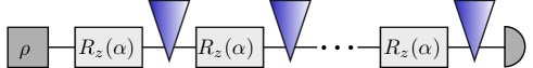
Figure 1: Schematic representation of the parameter encoding: Propagation starts on the left with an initial state $\rho$ and ends on the right with a measurement (semi-circle symbol). The encoding through linear precession $R_{z}(\alpha)$ about the $z$-axis by an angle $\alpha$ is periodically disrupted through parameter independent, non-linear, controlled kicks (blue triangles) that can render the system chaotic.

An experimental realization of the kicked top was proposed in haake2000can , including superradiant dissipation. It has been realized experimentally chaudhury2009quantum in cold cesium vapor using optical pulses (see Supplementary Note 1 for details).

Quantum parameter estimation theory

Quantum measurements are most conveniently described by a positive-operator valued measure (POVM) $\{\Pi_{\xi}\}$ with positive operators $\Pi_{\xi}$ (POVM-elements) that fulfill $\int d\xi\Pi_{\xi}=\mbox{\bf 1}$. Measuring a quantum state described by a density operator $\rho_{\alpha}$ yields for a given POVM and a given parameter $\alpha$ encoded in the quantum state a probability distribution $p_{\alpha}(\xi)={\rm tr}(\Pi_{\xi}\rho_{\alpha})$ of measurement results $\xi$. The Fisher information $I_{\text{Fisher},\alpha}$ is then defined by

$$I_{\text{Fisher},\alpha}:=\int d\xi\frac{(dp_{\alpha}(\xi)/d\alpha)^{2}}{p_{\alpha}(\xi)}\,.$$ (5)

The minimal achievable uncertainty, i.e. the variance of the estimator $\text{Var}(\alpha_{\text{est}})$, with which a parameter $\alpha$ of a state $\rho_{\alpha}$ can be estimated for a given POVM with $M$ independent measurements is given by the Cramér-Rao bound, $\text{Var}(\alpha_{\text{est}})\geq 1/(MI_{\text{Fisher},\alpha})$. Further optimization over all possible (POVM-)measurements leads to the quantum-Cramér-Rao bound (QCRB),

$$\text{Var}(\alpha_{\text{est}})\geq\frac{1}{MI_{\alpha}},$$ (6)

which presents an ultimate bound on the minimal achievable uncertainty, where $I_{\alpha}$ is the quantum Fisher information (QFI), and $M$ the number of independent measurements Helstrom1969 .

The QFI is related to the Bures distance $ds_{\rm Bures}^{2}$ between the states $\rho_{\alpha}$ and $\rho_{\alpha+d\alpha}$, separated by an infinitesimal change of the parameter $\alpha$, $ds_{\rm Bures}^{2}(\rho,\sigma)\equiv 2\left(1-\sqrt{F(\rho,\sigma)}\right)$. The fidelity $F(\rho,\sigma)$ is defined as $F(\rho,\sigma)=||\rho^{1/2}\sigma^{1/2}||^{2}_{1}$, and $||A||_{1}\equiv{\rm tr}\sqrt{AA^{\dagger}}$ denotes the trace norm Miszczak09 . With this,

$$I_{\alpha}=4ds_{\rm Bures}^{2}(\rho_{\alpha},\rho_{\alpha+d\alpha})/d\alpha^{2}$$ (7)

Braunstein94 . For pure states $\rho=|\psi\rangle\langle\psi|$, $\sigma=|\phi\rangle\langle\phi|$, the fidelity is simply given by $F(\rho,\sigma)=|\braket{\psi}{\phi}|^{2}$. A parameter coded in a pure state via the unitary transformation $|\psi_{\alpha}\rangle=e^{-i\alpha G}|\psi(0)\rangle$ with hermitian generator $G$ gives the QFI Braunstein90

$$I_{\alpha}=4\,\text{Var}(G)\equiv 4(\braket{G^{2}}-\braket{G}^{2})\,,$$ (8)

which holds for all $\alpha$, and where $\braket{\cdot}\equiv\langle\psi_{\alpha}|\cdot|\psi_{\alpha}\rangle$.

Loschmidt echo

The sensitivity to changes of a parameter of quantum-chaotic systems has been studied in great detail with the technique of Loschmidt echo Gorin06review , which measures the overlap $F_{\epsilon}(t)$ between a state propagated forward with a unitary operator $U_{\alpha}(t)$ and propagated backward with a slightly perturbed unitary operator $U_{\alpha+\epsilon}(-t)=U_{\alpha+\epsilon}^{\dagger}(t)$, where $U_{\alpha}(t)=T\exp\left(-\frac{i}{\hbar}\int_{0}^{t}dt^{\prime}H_{\alpha}(t^{\prime})\right)$ with the time ordering operator $T$, the Hamiltonian, $H_{\alpha+\epsilon}(t)=H_{\alpha}(t)+\epsilon V(t)$ and the perturbation $V(t)$,

$$F_{\epsilon}(t)=|\braket{\psi(0)}{U_{\alpha}(t)U_{\alpha+\epsilon}(-t)\psi(0)}|^{2}\,\,.$$ (9)

$F_{\epsilon}$ is exactly the fidelity that enters via the Bures distance in the definition eq. (7) of the QFI for pure states, such that $I_{\alpha}(t)=\lim_{\epsilon\to 0}4\frac{1-F_{\epsilon}(t)}{\epsilon^{2}}$.

Benchmarks

In order to assess the influence of the kicking on the QFI, we calculate as benchmarks the QFI for the (integrable) top with Floquet operator $U_{\alpha}(0)$ without kicking, both for an initial coherent state and for a Greenberger-Horne-Zeilinger (GHZ) state $|\psi_{\text{GHZ}}\rangle=(|j,j\rangle+|j,-j\rangle)/\sqrt{2}$. The latter is the equivalent of a NOON state written in terms of (pseudo-)angular momentum states. The QFI for the time evolution eq. (2) of a top with Floquet operator $U_{\alpha}(0)$ is given by eq. (8) with $G=J_{z}$. For an initial coherent state located at $\theta,\phi$ it results in a QFI

$$I_{\alpha}(t)=2t^{2}j\sin^{2}\theta.$$ (10)

As expected, $I_{\alpha}(t)=0$ for $\theta=0$ where the coherent state is an eigenstate of $U_{\alpha}(0)$. The scaling $\propto t^{2}$ is typical of quantum coherence, and $I_{\alpha}(t)\propto j$ signifies a SQL-type scaling with $N=2j$, when the spin-$j$ is composed of $N$ spin-$\frac{1}{2}$ particles in a state invariant under permutations of particles. For the benchmark we use the optimal value $\theta=\pi/2$ in eq. (10), i.e. $I_{\text{top,CS}}\equiv 2t^{2}j$. For a GHZ state, the QFI becomes

$$I_{\alpha}(t)=4t^{2}j^{2}\equiv I_{\text{top,GHZ}}\,,$$ (11)

which clearly displays the HL-type scaling $\propto(2j)^{2}\equiv N^{2}$.

Results for the kicked top without dissipation

In the fully chaotic case, known results for the Loschmidt echo suggest a QFI of the KT $\propto tj^{2}$ for times $t$ with $t_{E}<t<t_{H}$, where $t_{\text{E}}=\frac{1}{\lambda}\ln\left(\frac{\Omega_{\text{V}}}{h^{d}}\right)$ is the Ehrenfest time, and $t_{\text{H}}=\hbar/\Delta$ the Heisenberg time; $\lambda$ is the Lyapunov exponent, $\Omega_{\text{V}}$ the volume of phase-space, $h^{d}$ with $d$ the number of degrees of freedom the volume of a Planck cell, and $\Delta$ the mean energy level spacing zaslavsky1981stochasticity ; haake2013quantum ; Gorin06review . For the kicked top, $h^{d}\simeq\Omega_{\text{V}}/(2J)$. More precisely, we find for $t\simeq t_{E}$ a QFI $I_{\alpha}\propto tj^{2}$ and for $t\gg t_{H}$ (see Methods)

$$I(t)=8s\sigma_{\text{cl}}t^{2}J\,,$$ (12)

where $s$ denotes the number of invariant subspaces $s$ of the Hilbert space ($s=3$ for the kicked top with $\alpha=\pi/2$, see page 359 in Peres91 ), and $\sigma_{\text{cl}}$ is a transport coefficient that can be calculated numerically. The infinitesimally small perturbation relevant for the QFI makes that one is always in the perturbative regime PhysRevE.64.055203 ; PhysRevE.65.066205 . The Gaussian decay of Loschmidt echo characteristic of that regime becomes the slower the smaller the perturbation and goes over into a power law in the limit of infinitesimally small perturbation Gorin06review .

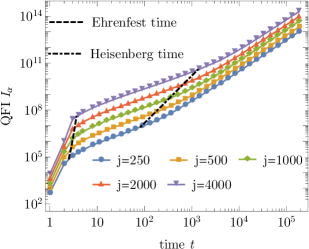
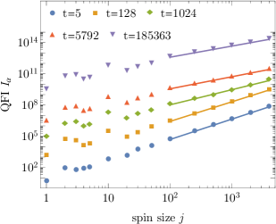
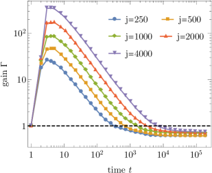
(a)                                                 (b)                                                  (c)

Figure 2: Quantum-chaotic enhancement of sensitivity. (a) $t$-scaling of the quantum Fisher information (QFI) $I_{\alpha}$ in the strongly chaotic case. Dashed and dash-dotted lines indicate Ehrenfest and Heisenberg times, respectively. (b) $j$-scaling of the QFI. Fits have slopes $1.96,1.88,1.46,1.16$, and $1.08$ in increasing order of $t$. (c) Gain $\Gamma=I_{\alpha,\textrm{KT}}/I_{\text{top,CS}}$ as function of time $t$ for different values of spin size $j$. The dashed black line marks the threshold $\Gamma=1$. Kicking strength $k=30$, and initial coherent state at $(\theta,\phi)=(\pi/2,\pi/2)$ in all plots.

The numerical results for the QFI in Fig. 2 illustrate a cross-over of power-law scalings in the fully chaotic case ($k=30$) for an initial coherent state located on the equator $(\theta,\phi)=(\pi/2,\pi/2)$. The analytical Loschmidt echo results are nicely reproduced: A smooth transition in scaling from $tj^{2}\rightarrow t^{2}j$ for $t=t_{\text{E}}\rightarrow t\gtrsim t_{\text{H}}$ can be observed and confirms eqs. (15),(16) in the Methods for $t>t_{\text{E}}=\ln(2J)/\lambda$, with the numerically determined Lyapunov exponent $\lambda\simeq 2.4733$, and eq. (12) for $t\gtrsim t_{\text{H}}\simeq J/3$ Gorin06review . We find for relatively large $j$ ($j\gtrsim 10^{2}$) a scaling $I_{\alpha}\propto j^{1.08}$ in good agreement with eq. (12) predicting a linear $j$-dependence for large $t\gtrsim t_{\text{H}}$. During the transient time $t<t_{\text{E}}$, when the state is spread over the phase space, QFI shows a rapid growth that can be attributed to the generation of coherences that are particularly sensitive to the precession.

The comparison of the KT’s QFI $I_{\alpha,\textrm{KT}}$ with the benchmark $I_{\text{top,CS}}$ of the integrable top in Fig. 2 (c) shows that a gain of more than two orders of magnitude for $j=4000$ can be found at $t\lesssim t_{\text{E}}$. Around $t_{\text{E}}$ the state has spread over the phase space and has developed coherences while for larger times $t>t_{\text{E}}$ the top catches up due to its superior time scaling ($t^{2}$ vs. $t$). The long-time behavior yields a constant gain less than 1, which means that the top achieves a higher QFI than the KT in this regime. The gain becomes constant as both top and KT exhibit a $t^{2}$ scaling of the QFI.

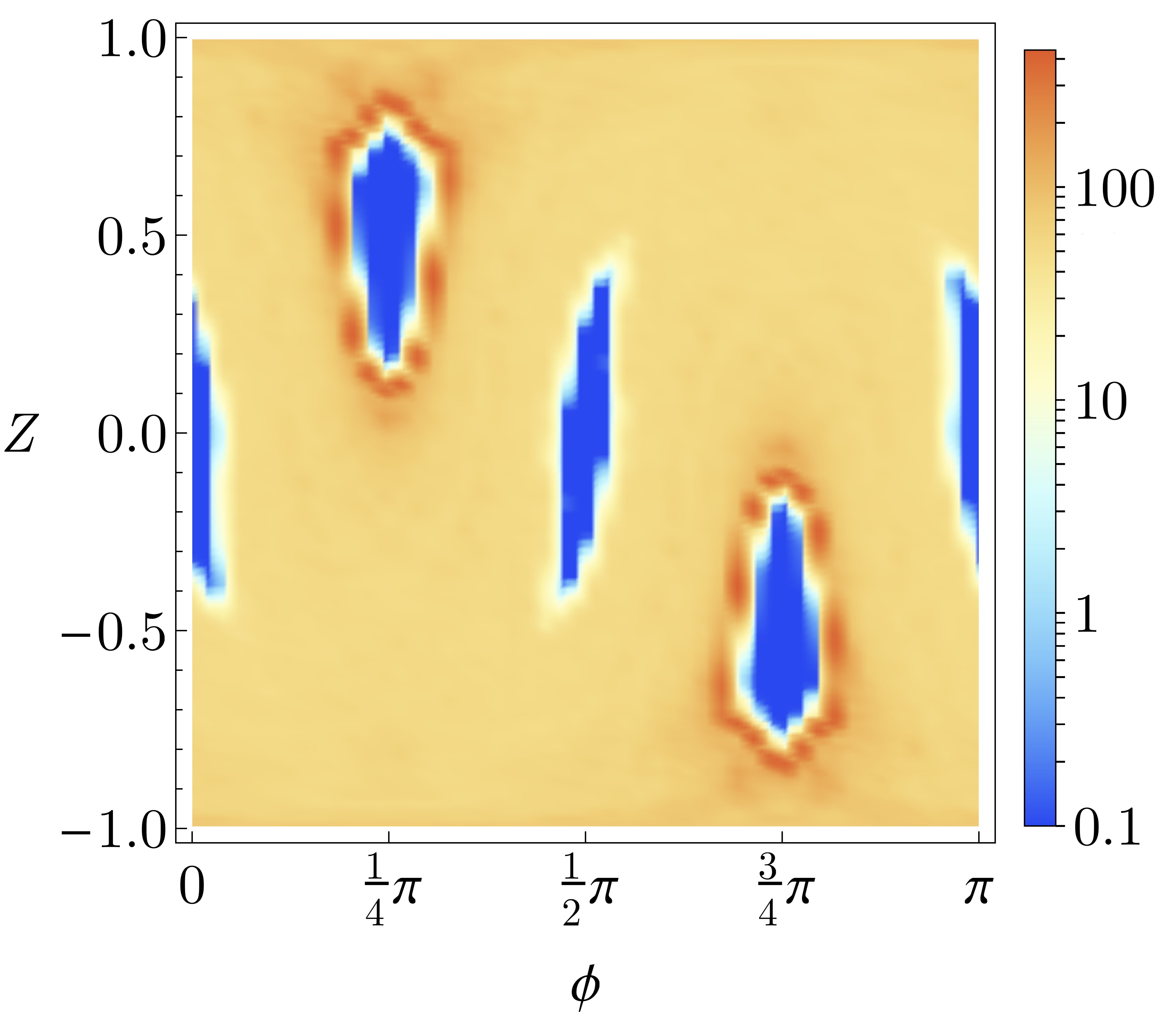
(a)                                                   (b)                                                   (c)

Figure 3: Portraits of a mixed phase space for large spin size $j=4000$. The heat maps depict quantum Fisher information (QFI) in panel (a) and gain $\Gamma$ in panel (b) at time $t=2^{15}$ and kicking strength $k=3$. $\Gamma<0.1$ is depicted as $\Gamma=0.1$ to simplify the representation. A gain of more than two orders of magnitude in the QFI is observed for edge states, localized on the border of the stability islands. For comparison, panel (c) depicts the classical Lyapunov exponent $\lambda$.

Whereas in the fully chaotic regime the memory of the initial state is rapidly forgotten, and the initial state can therefore be chosen anywhere in the chaotic sea without changing much the QFI, the situation is very different in the case of a mixed phase space, in which stability islands are still present. Fig. 3 shows phase space distributions for $k=3$ of QFI and gain $\Gamma=I_{\alpha,\textrm{KT}}/I_{\text{top,CS}}$ exemplarily for large $t$ and $j$ ($t=2^{15}$, $j=4000$) in comparison with the classical Lyapunov exponent, where $\phi,Z$ signify the position of the initial coherent state.

The QFI nicely reproduces the essential structure in classical phase space for the Lyapunov exponent $\lambda$ (see Methods for the calculation of $\lambda$). Outside the regions of classically regular motion, the KT clearly outperforms the top by more than two orders of magnitude. Remarkably, the QFI is highest at the boundary of non-equatorial islands of classically regular motion. Coherent states located on that boundary will be called edge states.

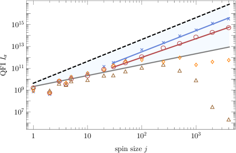
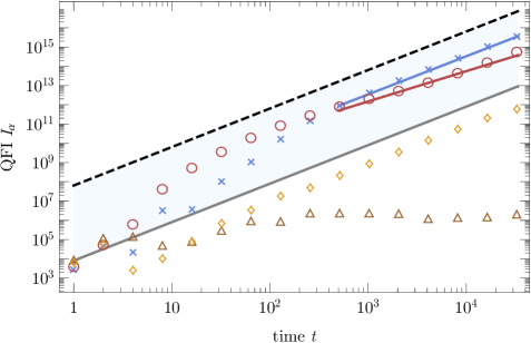
(a)                                                                             (b)

Figure 4: Scaling of quantum Fisher information (QFI) in different areas of a mixed phase space. QFI $I_{\alpha}(j)$ (panel (a) for time $t=2^{15}$) and $I_{\alpha}(t)$ (panel (b) for spin size $j=4000$) for kicking strength $k=3$ and different initial coherent states $|\theta,\phi\rangle$ (as marked in panel (a) of Figure 3): inside an equatorial (brown triangles, $|1.82,1.54\rangle$) and a non-equatorial (orange diamonds, $|2.20,2.44\rangle$) stability island, in the chaotic sea (red circles, $|2.46,0.32\rangle$), and an edge state (blue crosses, $|2.56,2.31\rangle$). Benchmarks $I_{\text{top,CS}}$ (gray line) and $I_{\text{top,GHZ}}$ (black dashed line) represent the standard quantum limit and Heisenberg limit, respectively. Fits for the edge state and the state in the chaotic sea exhibit a slope of $1.94$ and $1.71$ for the $j$-scaling, and $1.98$ and $1.57$ for the $t$-scaling.

The diverse dynamics for different phase space regions calls for dedicated analyses. Fig. 4 depicts the QFI with respect to $j$ and $t$. The blue area is lower and upper bounded by the benchmarks $I_{\text{top,CS}}$ and $I_{\text{top,GHZ}}$, eq. (11), respectively.

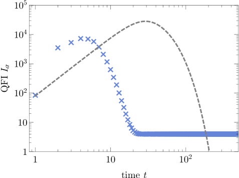
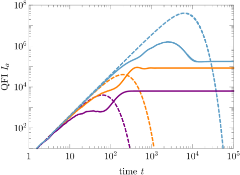
(a)                                                                            (b)
     
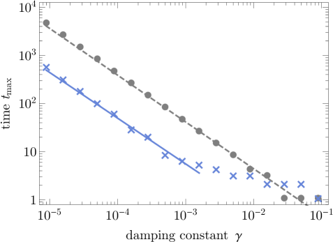
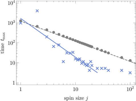
(c)                                                                            (d)

Figure 5: Time evolution of the quantum Fisher information (QFI) for the dissipative kicked top. In all subplots we look at an initial coherent state at $(\theta,\phi)=(\pi/2,\pi/2)$. (a) Exemplary behavior as function of time for a dissipative top (DT, dashed gray line) and a chaotic (kicking strength $k=30$) dissipative kicked top (DKT, blue crosses) for spin size $j=40$, damping constant $\gamma=0.5\times 10^{-3}$. (b) High plateau values of the QFI are achieved for $j=2$ and $k=30$ for various values of the damping constant ($\gamma=0.5\times 10^{-2}$ for the purple line, $\gamma=1.58\times 10^{-3}$ for the orange line, and $\gamma=0.5\times 10^{-4}$ for the blue line), while dashed lines represent corresponding QFI with $k=0$. (c,d) Time $t_{\text{max}}$ at which the QFI of the DT (gray dots) and DKT (blue crosses) reaches its maximum as function of $\gamma$ and $j$, respectively. The fits for the DT (gray line) exhibit a slope of $-0.97$ and $-1.01$, and the fits for the DKT (blue, dashed) a slope of $-0.95$ and $-1.94$ for scaling with $\gamma$ and $j$, respectively. Parameters $j=15$ in (c) and $\gamma=0.5\times 10^{-3}$ in (d). The plotted range of the fits corresponds to the fitted data.

We find that initial states in the chaotic sea perform best for small times while for larger times ($t\gtrsim 300$ for $j=4000$) edge states perform best. Note that this is numerically confirmed up to very high QFI values ($>10^{14}$). The superiority of edge states holds for $j\gtrsim 10$ for large times ($t\gtrsim 10^{3}$, see panel (a) in Fig. 4). Large values of $j$ allow one to localize states essentially within a stability island. A coherent state localized within a non-equatorial stability island shows a quadratic $t$-scaling analog to the regular top. For a state $|\psi_{\text{eq}}\rangle$ localized around a point within an equatorial island of stability the QFI drastically decays with increasing $j$ (brown triangles). The scaling with $t$ for $j=4000$ reveals that QFI does not increase with $t$ in this case, it freezes. One can understand the phenomenon as arising from a freeze of fidelity due to a vanishing time averaged perturbation Gorin06review ; sankaranarayanan2003recurrence : the dynamics restricts the states to the equatorial stability island with time average $\overline{\langle\psi_{\text{eq}}|(U_{\alpha}^{t})^{\dagger}(k){J_{z}}U_{\alpha}^{t}(k)|\psi_{\text{eq}}\rangle}=0$. This can be verified numerically, and contrasted with the dynamics when initial states are localized in the chaotic sea or on a non-equatorial island.

Results for the dissipative kicked top

For any quantum-enhanced measurement, it is important to assess the influence of dissipation and decoherence. We first study superradiant damping Dicke54 ; Bonifacio71a ; Haake73 ; Gross82 ; kaluzny1983observation as this enables a proof-of-principle demonstration with an analytically accessible propagator for the master equation with spins up to $j\simeq 200$ and correspondingly large gains. Then, in the next subsection, we show by detailed and realistic modeling including all the relevant decoherence mechanisms that sensitivity of existing state-of-the-art alkali-vapor-based spin-precession magnetometers in the spin-exchange-relaxation-free (SERF) regime can be enhanced by non-linear kicks.

At sufficiently low temperatures ($k_{B}T\ll\hbar\omega$, where $\hbar\omega$ is the level spacing between adjacent states $|jm\rangle$) superradiance is described by the Markovian master equation for the spin-density matrix $\rho(t)$ with continuous time,

$$\frac{d}{dt}\rho(t)=\gamma([J_{-},\rho(t)J_{+}]+[J_{-}\rho(t),J_{+}])\equiv\Lambda\rho(t)\,,$$ (13)

where $J_{\pm}\equiv J_{x}\pm iJ_{y}$, with the commutator $[A,B]=AB-BA$, and $\gamma$ is the dissipation rate, with the formal solution $\rho(t)=\exp(\Lambda t)\rho(0)\equiv D(t)\rho(0)$. The full evolution is governed by $d\rho(t)/dt=\Lambda\rho(t)-i\hbar[H_{\textrm{KT}}(t),\rho(t)]$. Dissipation and precession about the $z$-axis commute, $\Lambda(J_{z}\rho J_{z})=J_{z}(\Lambda\rho)J_{z}$. $\Lambda$ can therefore act permanently, leading to the propagator $P$ of $\rho$ from discrete time $t$ to $t+\tau$ for the dissipative kicked top (DKT) haake2013quantum ; Braun01B

$$\rho(t+\tau)=P\rho(t)=U_{\alpha}(k)\left(D(\tau)\rho(t)\right)U_{\alpha}^{\dagger}(k).$$ (14)

For the sake of simplicity we again set the period $\tau=1$, and $t$ is taken again as discrete time in units of $\tau$. Then, $\gamma\tau\equiv\gamma$ controls the effective dissipation between two unitary propagations. Classically, the DKT shows a strange attractor in phase space with a fractal dimension that reduces from $d=2$ at $\gamma=0$ to $d=0$ for large $\gamma$, when the attractor shrinks to a point attractor and migrates towards the ground state $|j,-j\rangle$ Braun01B . Quantum mechanically, one finds a Wigner function with support on a smeared out version of the strange attractor that describes a non-equilibrium steady state reached after many iterations. Such a non-trivial state is only possible through the periodic addition of energy due to the kicking. Because of the filigrane structure of the strange attractor, one might hope for relatively large QFI, whereas without kicking the system would decay to the ground state, where the QFI vanishes. Creation of steady non-equilibrium states may therefore offer a way out of the decoherence problem in quantum metrology, see also section V.C in Ref. braun2017without for similar ideas.

Vanishing kicking strength, i.e. the dissipative top (DT) obtained from the DKT by setting $k=0$, will serve again as benchmark. While in the dissipation-free regime we took the top’s QFI and with it its SQL-scaling ($\propto jt^{2}$) as reference, SQL-scaling no longer represents a proper benchmark, because damping typically corrupts QFI with increasing time. To illustrate the typical behavior of QFI we exemplarily choose certain spin sizes $j$ and damping constants $\gamma$ here and in the following, such as $j=40$ and $\gamma=0.5\times 10^{-3}$ in Fig. 5 (a), while computational limitations restrict us to $j\lesssim 200$.

Figure 5 shows the typical overall behavior of the QFI of the DT and DKT as function of time: After a steep initial rise $\propto t^{2}$, the QFI reaches a maximum whose value is the larger the smaller the dissipation. Then the QFI decays again, dropping to zero for the DT, and a plateau value for the DKT. The time at which the maximum value is reached decays roughly as $1/(j\gamma)$ for the DT, and as $1/j^{0.95}$ and $1/\gamma^{1.94}$ for the DKT. The plateau itself is in general relatively small for the limited values of $j$ that could be investigated numerically, but it should be kept in mind that i.) for the DT the plateau does not even exist (QFI always decays to zero for large time, as dissipation drives the system to the ground state $|j,-j\rangle$ which is an eigenstate of $J_{z}$ and hence insensitive to precession); and ii.), there are exceptionally large plateau values even for small $j$, see e.g. the case of $j=2$ in Fig. 5 (b). There, for $\gamma=1.58\times 10^{-3}$, the plateau value is larger by a factor $2.35$ than the DT’s QFI optimized over all initial coherent states for all times. Note that since $\Lambda(J_{z}\rho J_{z})=J_{z}(\Lambda\rho)J_{z}$, for the DT an initial precession about the $z$-axis that is part of the state preparation can be moved to the end of the evolution and does not influence the QFI of the DT. Optimizing over the initial coherent state can thus be restricted to optimizing over $\theta$.

When considering dynamics, it is natural also to include time as a resource. Indeed, experimental sensitivities are normally given as uncertainties per square root of Hertz: longer (classical) averaging reduces the uncertainty as $1/\sqrt{T_{\text{av}}}$ with averaging time $t=T_{\text{av}}$. For fair comparisons, one multiplies the achieved uncertainty with $\sqrt{T_{\text{av}}}$. Correspondingly, we now compare rescaled QFI and Fisher information, namely $I_{\alpha}^{(t)}\equiv I_{\alpha}/T_{\text{av}}$, $I_{\textrm{Fisher},\alpha}^{(t)}\equiv I_{\textrm{Fisher},\alpha}/T_{\textrm{av}}$. A protocol which reaches a given level of QFI more rapidly has then an advantage, and best precision corresponds to the maximum rescaled QFI or Fisher information, $\hat{I}_{\alpha}^{(t)}\equiv\max_{t}I^{(t)}_{\alpha}$ or $\hat{I}_{\textrm{Fisher},\alpha}^{(t)}\equiv\max_{t}I^{(t)}_{\textrm{Fisher},\alpha}$.

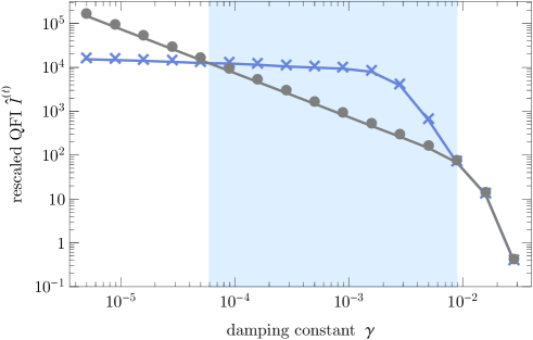
Figure 6: Enhancement in measurement precision through kicking (blue crosses) is found over a broad range of damping strengths. Comparison of the maximal rescaled quantum Fisher information $\hat{I}_{\alpha}^{(t)}$ for the dissipative top (gray dots) and the dissipative kicked top (blue crosses); kicking strength $k=30$ and spin size $j=100$. In both cases, $\hat{I}_{\alpha}^{(t)}$ was optimized over the location of initial coherent states. The blue-shaded area marks the range $1.2\lesssim 2\gamma J^{2}\lesssim 180$ where the reference is outperformed.

Figure 6 shows that in a broad range of dampings that are sufficiently strong for the QFI to decay early, the maximum rescaled QFI of the DKT beats that quantity of the DT by up to an order of magnitude. Both quantities were optimized over the location of the initial coherent states.

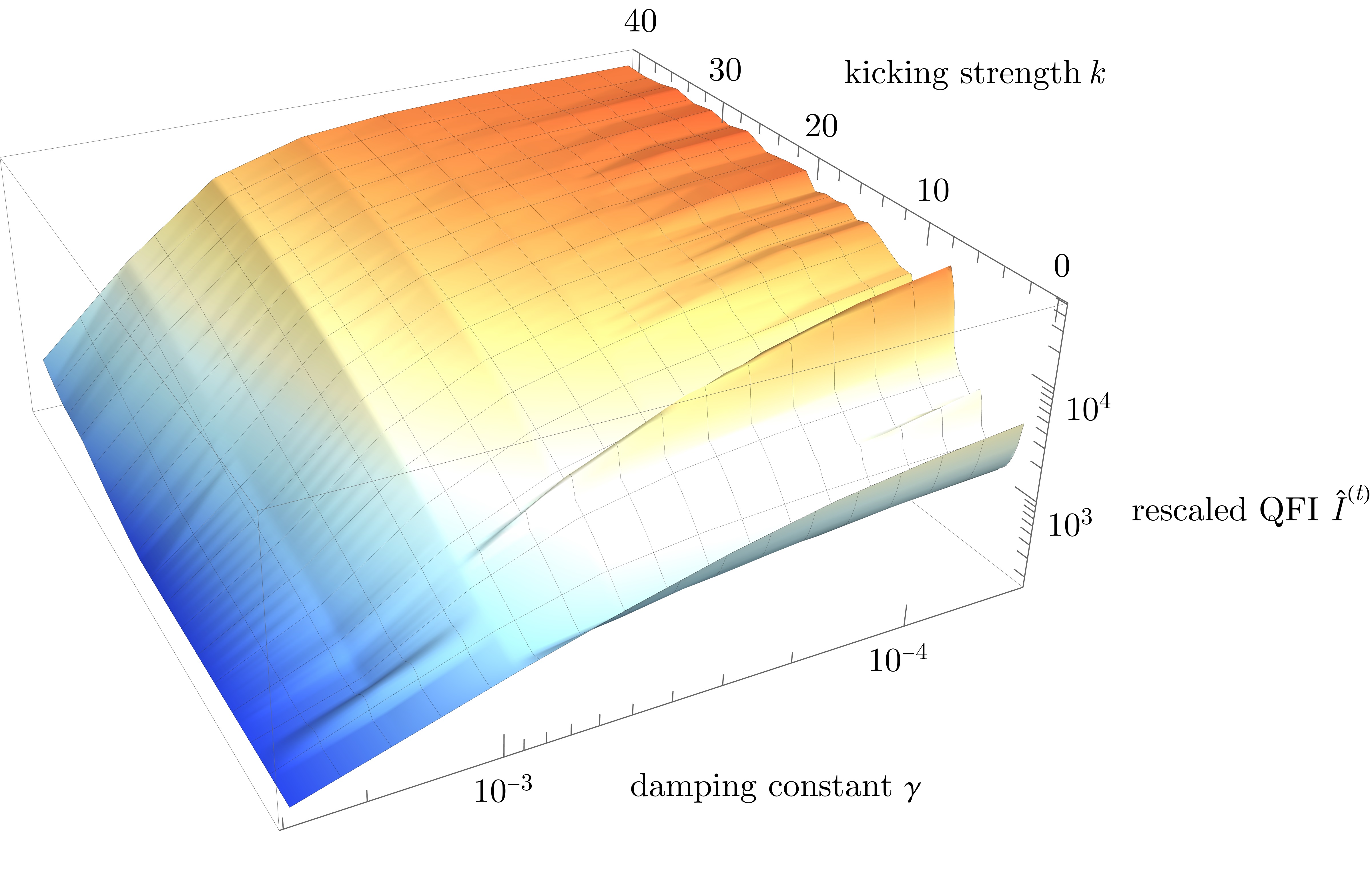
(a)                                                                             (b)

Figure 7: Rescaled quantum Fisher information (QFI) and gains in measurement precision. Rescaled QFI of the dissipative kicked top $\hat{I}^{(t)}_{\alpha,\textrm{DKT}}(\theta=\pi/2,\phi=\pi/2)$ in panel (a) and gain $\Gamma=\frac{\hat{I}_{\alpha,\textrm{DKT}}^{(t)}(\theta=\pi/2,\phi=\pi/2)}{\hat{I}_{\alpha,\text{DT}}^{(t)}}$ in panel (b) as function of damping constant $\gamma$ and kicking strength $k$ at $j=200$. Note that in this case $\hat{I}^{(t)}_{\alpha}$ is optimized over initial states only for the dissipative top.

Figure 7 shows $\hat{I}_{\alpha}^{(t)}$ and the gain in that quantity compared to the non-kicked case as function of both the damping and the kicking strength. One sees that in the intermediate damping regime ($\gamma\simeq 10^{-3}$) the gain increases with kicking strength, i.e. increasingly chaotic dynamics.

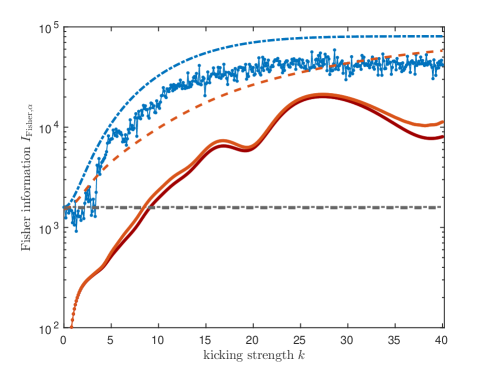
Figure 8: Performance of an exemplary spin-component measurement with superradiance damping. Fisher information $I_{\text{Fisher},\alpha}$ related to measuring the $y$-component of the spin, $J_{y}$, after $t=2$ time steps without dissipation (blue line) as well as in the presence of dissipation (bright red line, damping constant $\gamma=0.5\times 10^{-3}$), upper bounded by corresponding quantum Fisher informations (blue dash-dotted and red dashed lines), for spin size $j=200$, and an initial state at $(\theta,\phi)=(\pi/2,\pi/2)$. For the dissipative case Fisher information with a $5\%$ uncertainty in the kicking strength is given by the dark red line slightly below the bright red line. Horizontal gray lines represent benchmarks (kicking strength $k=0$) for $t=2$ optimized over initial states (dashed with dissipation and dash-dotted without; lines are almost on top of each other). In both cases the benchmark is clearly outperformed for $k\gtrsim 3.5$ and $k\gtrsim 10.6$ without and with dissipation, respectively.

For exploiting the enhanced sensitivity shown to exist through the large QFI, one needs also to specify the actual measurement of the probe. In principle the QCRB formalism allows one to identify the optimal POVM measurement if the parameter is known, but these may not always be realistic. In Fig. 8 we investigate $J_{y}$ as a feasible example for a measurement for a spin size $j=200$ after $t=2$ time steps. We find that there exists a broad range of kicking strengths where the reference (state-optimized but $k=0$) is outperformed in both cases, with and without dissipation. In a realistic experiment, control parameters such as the kicking strength are subjected to variations. A $5\%$ variance in $k$, which was reported in Ref. chaudhury2009quantum , reduces the Fisher information only marginally and does not challenge the advantage of kicking. This can be calculated by rewriting the probability that enters in the Fisher information in eq. (5) according to the law of total probability, $p_{\alpha}(\xi)=\int dk\,p(k)p_{\alpha}(\xi|k)$ where $p(k)$ is an assumed Gaussian distribution of $k$ values with $5\%$ variance and $p_{\alpha}(\xi|k)={\rm tr}[\Pi_{\xi}\rho_{\alpha}(k)]$ with $\Pi_{\xi}$ a POVM element and $\rho_{\alpha}(k)$ the state for a given $k$ value. The advantage from kicking remains when investigating a rescaled and time-optimized Fisher information (not shown in Fig. 8).

Improving a SERF magnetometer

We finally show that quantum-chaotically enhanced sensitivity can be achieved in state-of-the-art magnetometers by investigating a rather realistic and detailed model of an alkali-vapor-based spin-precession magnetometer acting in the SERF regime. SERF magentometers count amongst the most sensitive magnetometers for detecting small quasi-static magnetic fields allred2002high ; Kominis03 ; savukov2005effects ; budker2007optical ; sheng2013subfemtotesla . We consider a cesium-vapor magnetometer at room temperature in the SERF regime similar to experiments with rubidium in Ref. balabas2010polarized . Kicks on the single cesium-atom spins can be realized as in Ref. chaudhury2009quantum by exploiting the spin-dependent rank-2 (ac Stark) light-shift generated with the help of an off-resonant laser pulse. Typical SERF magnetometers working at higher temperatures with high buffer-gas pressures exhibit an unresolved excited state hyperfine splitting due to pressure broadening, which makes kicks based on rank-2 light-shifts ineffective. Dynamics are modeled in the electronic ground state $6^{2}\text{S}_{1/2}$ of ¹³³Cs that splits into total spins of $f=3$ and $f=4$, where kicks predominantly act on the $f=3$ manifold.

The model is quite different from the foregoing superradiance model because of a different decoherence mechanism originating from collisions of Cs atoms in the vapor cell: We include spin-exchange and spin-destruction relaxation, as well as additional decoherence induced by the optical implementation of the kicks. With this implementation of kicks one is confined to a small spin size $f=3$ of single atoms, such that the large improvements in sensitivity found for the large spins discussed above cannot be expected. Nevertheless, we still find a clear gain in the sensitivity and an improved robustness to decoherence due to kicking. Details of the model described with a master equation appelt1998theory ; deutsch2010quantum can be found in the Supplementary Note 2.

Spins of cesium atoms are initially pumped into a state spin-polarized in $z$-direction orthogonal to the magnetic field $\textbf{B}=B\hat{\textbf{y}}$ in $y$-direction, whose strength $B$ is the parameter $\alpha$ to be measured. We let spins precess in the magnetic field, and, by incorporating small kicks about the $x$-axis, we find an improvement over the reference (without kicks) in terms of rescaled QFI and the precision based on the measurement of the electron-spin component $S_{z}$ orthogonal to the magnetic field. The best possible measurement precision $\Delta B$ in units of T$/\sqrt{\textrm{Hz}}$ per $1\,\textrm{cm}^{3}$ vapor volume is $\Delta B=1/\sqrt{nI_{B}^{(t)}}$ where $n\simeq 2\times 10^{10}$ is the number of cesium atoms in $1\,\textrm{cm}^{3}$. For a specific measurement, $I_{B}^{(t)}$ must be replaced by the corresponding rescaled Fisher information $I_{\textrm{Fisher, B}}^{(t)}$. We compare the models with and without kick directly on the basis of the Fisher information rather than modeling in addition the specific optical implementation and the corresponding noise of the measurement of $S_{z}$. Neglecting this additional read-out-specific noise leads to slightly better precision bounds than given in the literature, but does not distort the comparison.

The magnetic field was set to $B=4\times 10^{-14}\,\textrm{T}$ in $y$-direction, such that the condition for the SERF regime is fulfilled, i.e. the Larmor frequency is much smaller than the spin-exchange rate, and the period is set to $\tau=1\,$ms. Since kicks induce decoherence in the atomic spin system, we have to choose a very small effective kicking strength of $k\simeq 6.5\times 10^{-4}$ for the kicks around the $x$-axis (with respect to the $f=3$ ground-state manifold), generated with an off-resonant $2\,\mu$s light pulse with intensity $I_{\text{kick}}=0.1\,$mW/cm² linearly polarized in $x$-direction, to find an advantage over the reference.

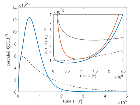
Figure 9: Performance of a magnetic-field measurement with a kicked atomic-vapor magnetometer. While the gray dashed line shows the rescaled quantum Fisher information $I^{(t)}_{B}$ for measuring the magnetic field $B$ with an spin-exchange-relaxation-free magnetometer, the blue line is obtained by adding a short optical kick at the end of each period $\tau$. The inset shows precision $\Delta B$ in units of T per $\sqrt{\text{Hz}}$ for an optimal measurement (gray dashed line and blue line without and with kicks, respectively) and for measuring the $z$-component of the electronic spin $S_{z}$ (grey dash-dotted and red line without and with kicks, respectively).

The example of Fig. 9 shows about $31\%$ improvement in measurement precision $\Delta B$ for an optimal measurement (QFI, upper right inset) and $68\%$ improvement in a comparison of $S_{z}$ measurements (inset), which is impressive in view of the small system size.The achievable measurement precision of the kicked dynamics exhibits an improved robostness to decoherence: rescaled QFI for the kicked dynamics continues to increase and sets itself apart from the reference around the coherence time associated with spin-destruction relaxation. The laser light for these pulses can be provided by the laser used for the read out, which is typically performed with an off-resonant laser. A further improvement in precision is expected from additionally measuring kick pulses for readout or by applying kicks not only to the $f=3$ but also to the $f=4$ ground-state manifold of ¹³³Cs. Further, it might be possible to dramatically increase the relevant spin-size by applying the kicks to the joint spin of the cesium atoms, for instance, through a double-pass Faraday effect takeuchi2005spin .

Discussion

Rendering the dynamics of quantum sensors chaotic allows one to harvest a quantum enhancement for quantum metrology without having to rely on the preparation or stabilization of highly entangled states. Our results imply that existing magnetic field sensors budker2007optical ; ledbetter2008spin based on the precession of a spin can be rendered more sensitive by disrupting the time-evolution by non-linear kicks. The enhancement persists in rather broad parameter regimes even when including the effects of dissipation and decoherence. Besides a thorough investigation of superradiance damping over large ranges of parameters, we studied a cesium-vapor-based atomic magnetomter in the SERF regime based on a detailed and realistic model allred2002high ; Kominis03 ; savukov2005effects ; budker2007optical ; balabas2010polarized . Although the implementation of the non-linearity via a rank-2 light shift introduces additional decoherence and despite the rather small atomic spin size $f\leq 4$, a considerable improvement in measurement sensitivity is found ($68\%$ for a read-out scheme based on the measurement of the electronic spin-component $S_{z}$). The required non-linearity that can be modulated as function of time has been demonstrated experimentally in chaudhury2009quantum in cold cesium vapor.

Even higher gains in sensitivity are to be expected if an effective interaction can be created between the atoms, as this opens access to larger values of total spin size for the kicks. This may be achieved e.g. via a cavity as suggested for pseudo-spins in agarwal1997atomic , or the interaction with a propagating light field as demonstrated experimentally in takeuchi2005spin ; Julsgaard01 with about $10^{12}$ cesium atoms. More generally, our scheme will profit from the accumulated knowledge of spin-squeezing, which is also based on the creation of an effective interaction between atoms. Finally, we expect that improved precision can be found in other quantum sensors that can be rendered chaotic as well, as the underlying sensitivity to change of parameters is a basic property of quantum-chaotic systems.

Methods

QFI for kicked time-evolution of a pure state

The QFI in the chaotic regime with large system dimension $2J$ and times larger than the Ehrenfest time, $t>t_{\text{E}}$, is given in linear-response theory by an auto-correlation function $C(t)\equiv\braket{\tilde{V}(t)\tilde{V}(0)}-\braket{\tilde{V}(t)}\braket{\tilde{V}(0)}$ of the perturbation of the Hamiltonian in the interaction picture, $H_{\alpha+\epsilon}(t)=H_{\alpha}(t)+\epsilon V(t)$, $\tilde{V}(t)=U_{\alpha}(-t)V(t)U_{\alpha}(t)$:

$$I_{\alpha}(t)=4\left(tC(0)+2\sum_{t^{\prime}=0}^{t-1}(t-t^{\prime})C(t^{\prime})\right).$$ (15)

In our case, the perturbation $V(t)=J_{z}$ is proportional to the parameter-encoding precession Hamiltonian, and the first summand in eq. (15) can be calculated for an initial coherent state,

$$C(0)=\frac{1}{3}j(j+1),$$ (16)

giving a $tj^{2}$-scaling starting from $t_{\text{E}}$. Due to the finite Hilbert-space dimension of the kicked top, the auto-correlation function decays for large times to a finite value $\bar{C}$, leading to a term quadratic in $t$ from the sum in eq. (15) that simplifies to $I_{\alpha}=4\overline{C}t^{2}$ for $t\gg t_{H}$. If one rescales $J_{z}\rightarrow J_{z}/J$ such that it has a well defined classical limit, random matrix theory allows one to estimate the average value of $C(t)$ for large times: $\bar{C}=2Js\sigma_{\text{cl}}$, and $\sigma_{\text{cl}}$ is a transport coefficient that can be calculated numerically Gorin06review . This yields eq. (12).

Lyapunov exponent

A data point located at $(Z,\phi)$ for the Lyapunov exponent in Fig. 2 (c) was obtained numerically by averaging over $100$ initial conditions equally distributed within a circular area of size $1/j$ (corresponding to the coherent state) centered around $(Z,\phi)$.

Data availability

Relevant data is also available from the authors upon request.

References

End notes

Acknowledgements

This work was supported by the Deutsche Forschungsgemeinschaft (DFG), Grant No. BR 5221/1-1. Numerical calculations were performed in part with resources supported by the Zentrum für Datenverarbeitung of the University of Tübingen.

Author Contribution

D. B. initiated the idea and L. F. made the calculations and numerical simulations. Both Authors contributed to the interpretation of data and the writing of the manuscript.

Competing Interests

The authors declare no competing interests.

Supplementary Information

Supplementary Note 1. Realization of the kicked top

The kicked top (KT) has been realized experimentally by Chaudhury et al. chaudhury2009quantumsup using the atomic spin of a ${}^{133}\textrm{Cs}$ atom in the $f=3$ hyperfine ground state. Linear precession of the spin was implemented through magnetic pulses, and the torsion through an off-resonant laser field that exploited a spin-dependent rank-2 (ac Stark) light shift.

An implementation of the KT using microwave superradiance was proposed by Haake haake2000cansup : The top is represented by the collective pseudo-spin of $N$ two-level atoms coupled with the same coupling constant to a single mode of an electromagnetic field in a cavity, with a controlled detuning between mode and atomic frequencies. Large detuning compared to the Rabi frequency $\Omega=g\sqrt{N}$ with coupling strength $g$ allows one to adiabatically eliminate the cavity mode and leads to an effective interaction of the type $J_{z}^{2}$ agarwal1997atomicsup (replacing our $J_{y}^{2}$), while superradiant damping as described by the master equation (13) in the main text for the reduced density operator of the atoms can still prevail haake2000cansup . Finally, a linear rotation about the $x$-axis can be achieved through resonant microwave pulses, replacing the linear precession about the $z$-axis of the KT. The parameter $\alpha$ is now proportional to the Rabi frequency of the microwave pulse.

Supplementary Note 2. Spin-exchange-relaxation-free Cs-vapor magnetometer

Adapting standard notation in atomic physics, atomic spin operators will be denoted in the following by $\textbf{F}=(F_{x},F_{y},F_{z})$ with spin size $f$, $F_{z}|fm\rangle=m|fm\rangle$, and total electronic angular momentum $\textbf{J}=\textbf{L}+\textbf{S}$ with quantum number $j$, composed of orbital angular momentum L and electron spin S. We model a room-temperature spin-exchange-relaxation-free (SERF) Cs-vapor magnetometer similar to the experiments with Rb-vapor of Balabas et al. balabas2010polarizedsup . The Cs spin sensitive to the magnetic field $B$ is composed of a nuclear spin $K=7/2$ and one valence electron with an electronic spin $s=1/2$ which splits the ground state $6^{2}\text{S}_{1/2}$ into two energy levels with total spin $f_{1}=3$ and $f_{2}=4$. This results in an effective Hilbert space of dimension $2(2K+1)=16$ for our model of a kicked SERF magnetometer.

The dominant damping mechanisms are related to collisions of cesium atoms with each other and with the walls of the vapor cell.

In the SERF regime the spin-exchange rate is much greater than the rate of Larmor precession, typically realized by very small magnetic fields, a high alkali-atom density ($10^{13}$ atoms per cm³), high buffer-gas pressure, and heating of the vapor cell. Then, spin-exchange relaxation is so strong, that the population of hyperfine ground levels ($f_{i}=3,4$) is well described by a spin-temperature distribution. Here, we model a SERF magnetmeter with a lower alkali-atom density of $2\times 10^{10}$ atoms per cm³ without buffer gas at room temperature $T=294.13\,$K. Modern alkene-based vapor-cell coatings support up to $10^{6}$ collisions before atoms become depolarized balabas2010polarizedsup . For a spherical vapor-cell with a $1.5\,$cm radius it follows that collisions with walls limit the lifetime of spin polarization to $T_{\textrm{wall}}\simeq 92\,$s. Since the effect of collisions among Cs atoms leads to stronger depolarization we neglect collisions with the walls in our model.

While the typical treatment proceeds by eliminating the nuclear-spin component we are interested in a dynamics that exploits the larger Hilbert space of the Cs spin. Therefore the evolution of the spin density matrix $\rho$ is described by a master equation that includes damping originating from collisions of Cs atoms appelt1998theorysup and an interaction with an off-resonant light field in the low-saturation limit deutsch2010quantumsup modeling the kicks:

$$\frac{d\rho}{dt} =R_{\textrm{se}}\left[\varphi(1+4\braket{\textbf{S}}\cdot\textbf{S})-\rho\right]+R_{\text{sd}}\left[\varphi-\rho\right]+a_{\textrm{hf}}\frac{[\textbf{K}\cdot\textbf{S},\rho]}{i\hbar}+\frac{H_{A}^{\text{eff}}\rho-\rho H_{A}^{\text{eff}\dagger}}{i\hbar}$$

$$\quad+\gamma_{\text{nat}}\sum_{q=-1}^{1}\left(\sum_{f,f_{1}}W_{q}^{ff_{1}}\rho_{f_{1}f_{1}}\left(W_{q}^{ff_{1}}\right)^{\dagger}+\sum_{f_{1}\neq f_{2}}W_{q}^{f_{2}f_{2}}\rho_{f_{2}f_{1}}\left(W_{q}^{f_{1}f_{1}}\right)^{\dagger}\right)$$ (17)

The first two summands describe spin-exchange relaxation and spin-destruction relaxation, respectively, where $R_{\text{se}}$ denotes the spin-exchange rate and $R_{\text{sd}}$ the spin-destruction rate, and $\varphi=\rho/4+\textbf{S}\cdot\rho\textbf{S}$ is called the purely nuclear part of the density matrix, where the electron-spin operator S only acts on the electron-spin component with expectation value $\braket{\textbf{S}}={\rm tr}[\textbf{S}\rho]$. The third summand is the hyperfine coupling of nuclear spin K and electronic spin S with hyperfine structure constant $a_{\text{hf}}$, and the fourth summand drives the dynamic with an effective non-hermitian Hamiltonian on both ground-state hyperfine manifolds $H_{A}^{\text{eff}}=H_{A,f=3}^{\text{eff}}+H_{A,f=4}^{\text{eff}}$, with

$$H_{A,f}^{\text{eff}}=\hbar\Omega_{\text{Lar}}F_{y}+\sum_{f^{\prime}}\frac{\hbar\Omega^{2}C_{j^{\prime}f^{\prime}f}^{(2)}}{4(\Delta_{ff^{\prime}}+i\gamma_{\text{nat}}/2)}\left|\bm{\epsilon_{\text{L}}}\cdot\textbf{F}\right|^{2}$$ (18)

that includes Larmor precession with frequency $\Omega_{\text{Lar}}=g_{f}\mu_{B}B/\hbar$ (with the Landé g-factor $g_{f}$ and the Bohr magneton $\mu_{B}$) of the atomic spin in the external magnetic field $\textbf{B}=B\hat{\textbf{y}}$, and the rank-2 light-shift induced by a light pulse that is linearly polarized with unit polarization vector $\bm{\epsilon}_{\text{L}}$ of the light field and off-resonant with detuning $\Delta_{ff^{\prime}}$ from the D1-line transition with $f\rightarrow f^{\prime}$. Further, we have the characteristic Rabi frequency $\Omega=\gamma_{\text{nat}}\sqrt{I_{\text{kick}}/(2I_{\text{sat}})}$ of the D1 line, the natural line width $\gamma_{\text{nat}}$, kick-laser intensity $I_{\text{kick}}$, saturation intensity $I_{\text{sat}}$, and the coefficient

$$C_{j^{\prime}f^{\prime}f}^{(2)}=(-1)^{3f-f^{\prime}}\frac{\sqrt{30}(2f^{\prime}+1)}{\sqrt{f(f+1)(2f+1)(2f-1)(2f+3)}}\left\{\begin{matrix}f&1&f^{\prime}\\ 1&f&2\end{matrix}\right\}\left|o_{1/2f}^{j^{\prime}f^{\prime}}\right|^{2},$$ (19)

where the curly braces denote the Wigner $6j$ symbol and

$$o_{jf}^{j^{\prime}f^{\prime}}=(-1)^{f^{\prime}+1+j^{\prime}+K}\sqrt{(2j^{\prime}+1)(2f+1)}\left\{\begin{matrix}f&K&j^{\prime}\\ j&1&f\end{matrix}\right\},$$ (20)

where total angular momentum of ground and excited levels of the D1 line are $j=j^{\prime}=1/2$. Photon scattering is taken into account by the imaginary shift of $\Delta_{ff^{\prime}}$ in the effective Hamiltonian and by the remaining parts of the master equation that correspond to optical pumping which leads to cycles of excitation to the 6P_1/2 manifold and spontaneous emission to the ground-electronic manifold 6S_1/2. When the laser is switched off the master equation solely involves the first four summands where $H_{A}^{\text{eff}}$ reduces to the Larmor precession term.

The jump operators are given as

$$W_{q}^{f_{b}f_{a}}=\sum_{f^{\prime}=3}^{4}\frac{\Omega/2}{\Delta_{f_{a}f^{\prime}}+i\gamma_{\text{nat}}/2}\left(\textbf{e}_{q}^{*}\cdot\textbf{D}_{f_{b}f^{\prime}}\right)\left(\bm{\epsilon}_{\textrm{L}}\cdot\textbf{D}_{f_{a}f^{\prime}}^{\dagger}\right),$$ (21)

with the spherical basis $\textbf{e}_{1}=-(\hat{\textbf{x}}+i\hat{\textbf{y}})/\sqrt{2}$, $\textbf{e}_{0}=\hat{\textbf{z}}$, $\textbf{e}_{-1}=(\hat{\textbf{x}}-i\hat{\textbf{y}})/\sqrt{2}$ in the Cartesian basis $\hat{\textbf{x}},\hat{\textbf{y}},\hat{\textbf{z}}$, and the raising operator $\textbf{D}^{\dagger}_{ff^{\prime}}=\sum_{q,m,m^{\prime}}\textbf{e}_{q}^{*}o_{jf}^{j^{\prime}f^{\prime}}\braket{f^{\prime}m^{\prime}}{fm;1q}|f^{\prime}m^{\prime}\rangle\langle fm|$ with Clebsch-Gordan coefficients $\braket{f^{\prime}m^{\prime}}{fm;1q}$ and magnetic quantum numbers $m$, $m^{\prime}$.

Excited state hyperfine levels are Doppler and pressure broadened, but we neglect pressure broadening which is much smaller than Doppler broadening due to the very low vapor pressure. Doppler broadening is taken into account by numerically averaging the righthand side of the master equation (Supplementary Equation Supplementary Note 2. Spin-exchange-relaxation-free Cs-vapor magnetometer) over the Maxwell-Boltzmann distribution of velocities of an alkali atom. This translates into an average over detunings $\Delta_{ff^{\prime}}$. Since $\Delta\gg\Omega$ must hold within the description of this master equation, we limit averaging over detunings to a $3\sigma$ interval.

By numerically solving the non-linear trace-preserving master equation (Supplementary Equation Supplementary Note 2. Spin-exchange-relaxation-free Cs-vapor magnetometer) with the Euler method (analog to Ref. savukov2005effectssup we take hyperfine coupling into account by setting off-diagonal blocks of the density matrix in the coupled $|fm\rangle$-basis after each Euler step to zero, because they oscillate very quickly with $a_{\text{hf}}$), we simulate dynamics similar to the dissipative kicked top described above with the difference that kicks are not assumed to be arbitrarily short, i.e. kicks and precession coexist during a light pulse. Kicks and corresponding dissipation are factored in by applying a superoperator to the state in each Euler step during a kick.

Spin-exchange and spin-destruction rates are estimated to $R_{\textrm{se}}\simeq 12\,$Hz and $R_{\textrm{sd}}\simeq 0.12\,$Hz from the known cross sections of Cs-Cs collisions, the mean relative thermal velocity of Cs atoms and their density.

For the concrete example of Fig. 7 we calculate with $2\times 10^{10}$ Cs atoms per $1\,$cm³ vapor volume, and kick laser pulses linearly polarized in $x$-direction, $\bm{\epsilon}_{\textbf{L}}=\textbf{x}$, with intensity $I_{\text{kick}}=0.1\,\text{mW/cm}^{2}$ and detuning halfway between the two components of the D1 line, and $\Delta_{34}\simeq-584\,\textrm{MHz}$. The period is $\tau=1\,\textrm{ms}$ where during the last $2\,\mu$s of each period the laser pulse is applied (effective kicking strength for the lower hyperfine level of the ground state is $k\simeq 6.5\times 10^{-4}$). We choose a small magnetic field $B=40\,$fT in $y$-direction so that we are well within the SERF regime, $R_{\textrm{se}}\gg\Omega_{\textrm{Lar}}$.

With a circular polarized pump beam in $z$-direction resonant with the D1 line the initial spin-state is polarized which in the presence of spin-relaxation leads to an effective thermal state

$$\rho=\frac{e^{\beta K_{z}}e^{\beta S_{z}}}{Z_{K}Z_{S}},$$ (22)

with the partition sum $Z_{j}=\sum_{m=-j}^{j}e^{\beta m}$ and $\beta=\ln\frac{1+q}{1-q}$, with polarization $q=0.95$. The readout is accomplished typically with the help of an off-resonant probe beam by measuring its polarization after it experienced a Faraday rotation when interacting with the atomic spin ensemble.

Supplementary References

References

- (1) Huelga, S. F. et al. Improvement of Frequency Standards with Quantum Entanglement. Phys. Rev. Lett. 79, 3865–3868 (1997).
- (2) Meyer, V. et al. Experimental Demonstration of Entanglement-Enhanced Rotation Angle Estimation Using Trapped Ions. Phys. Rev. Lett. 86, 5870–5873 (2001).
- (3) Leibfried, D. et al. Toward Heisenberg-Limited Spectroscopy with Multiparticle Entangled States. Science 304, 1476–1478 (2004).
- (4) Wasilewski, W. et al. Quantum Noise Limited and Entanglement-Assisted Magnetometry. Phys. Rev. Lett. 104, 133601 (2010).
- (5) Koschorreck, M., Napolitano, M., Dubost, B. & Mitchell, M. W. Sub-Projection-Noise Sensitivity in Broadband Atomic Magnetometry. Phys. Rev. Lett. 104, 093602 (2010).
- (6) Goda, K. et al. A quantum-enhanced prototype gravitational-wave detector. Nature Physics 4, 472–476 (2008).
- (7) Aasi, J. et al. Enhanced sensitivity of the LIGO gravitational wave detector by using squeezed states of light. Nature Photonics 7, 613–619 (2013).
- (8) Giovannetti, V., Lloyd, S. & Maccone, L. Quantum-enhanced positioning and clock synchronization. Nature 412, 417–419 (2001).
- (9) Allen, E. H. & Karageorgis, M. Radar systems and methods using entangled quantum particles (2008). US Patent 7,375,802.
- (10) Taylor, J. et al. High-sensitivity diamond magnetometer with nanoscale resolution. Nature Physics 4, 810–816 (2008).
- (11) Boto, A. N. et al. Quantum Interferometric Optical Lithography: Exploiting Entanglement to Beat the Diffraction Limit. Phys. Rev. Lett. 85, 2733–2736 (2000).
- (12) Higgins, B. L., Berry, D. W., Bartlett, S. D., Wiseman, H. M. & Pryde, G. J. Entanglement-free Heisenberg-limited phase estimation. Nature 450, 393–396 (2007).
- (13) Nagata, T., Okamoto, R., O’Brien, J. L. & Takeuchi, K. S. S. Beating the Standard Quantum Limit with Four-Entangled Photons. Science 316, 726–729 (2007).
- (14) Pezzè, L., Smerzi, A., Oberthaler, M. K., Schmied, R. & Treutlein, P. Quantum metrology with nonclassical states of atomic ensembles. eprint Preprint at https://arxiv.org/abs/1609.01609v2 (2016).
- (15) Peres, A. In Cerdeira, H. A., Ramaswamy, R., Gutzwiller, M. C. & Casati, G. (eds.) Quantum Chaos (World Scientific, Singapore, 1991).
- (16) Gorin, T., Prosen, T., Seligman, T. H. & Žnidarič, M. Dynamics of Loschmidt echoes and fidelity decay. Physics Reports 435, 33–156 (2006).
- (17) Boixo, S. et al. Quantum Metrology: Dynamics versus Entanglement. Phys. Rev. Lett. 101, 040403 (2008).
- (18) Xiao-Qian, W., Jian, M., Xi-He, Z. & Xiao-Guang, W. Chaos and quantum Fisher information in the quantum kicked top. Chinese Physics B 20, 050510 (2011).
- (19) Song, L., Ma, J., Yan, D. & Wang, X. Quantum Fisher information and chaos in the Dicke model. The European Physical Journal D 66, 201 (2012).
- (20) Weiss, C. & Teichmann, N. Signatures of chaos-induced mesoscopic entanglement. Journal of Physics B: Atomic, Molecular and Optical Physics 42, 031001 (2009).
- (21) Fröwis, F., Sekatski, P. & Dür, W. Detecting Large Quantum Fisher Information with Finite Measurement Precision. Phys. Rev. Lett. 116, 090801 (2016).
- (22) Macrì, T., Smerzi, A. & Pezzè, L. Loschmidt echo for quantum metrology. Phys. Rev. A 94, 010102 (2016).
- (23) Linnemann, D. et al. Quantum-Enhanced Sensing Based on Time Reversal of Nonlinear Dynamics. Phys. Rev. Lett. 117, 013001 (2016).
- (24) Ma, J., Wang, X., Sun, C. & Nori, F. Quantum spin squeezing. Physics Reports 509, 89–165 (2011).
- (25) Madhok, V., Riofrío, C. A., Ghose, S. & Deutsch, I. H. Information Gain in Tomography–A Quantum Signature of Chaos. Phys. Rev. Lett. 112, 014102 (2014).
- (26) Madhok, V., Riofrio, C. A. & Deutsch, I. H. Review: Characterizing and quantifying quantum chaos with quantum tomography. Pramana 87, 65 (2016).
- (27) Braun, D. et al. Quantum enhanced measurements without entanglement. eprint Preprint at https://arxiv.org/abs/1701.05152 (2017).
- (28) Allred, J., Lyman, R., Kornack, T. & Romalis, M. High-Sensitivity Atomic Magnetometer Unaffected by Spin-Exchange Relaxation. Phys. Rev. Lett. 89, 130801 (2002).
- (29) Kominis, I. K., Kornack, T. W., Allred, J. C. & Romalis, M. V. A subfemtotesla multichannel atomic magnetometer. Nature 422, 596––599 (2003).
- (30) Savukov, I. & Romalis, M. Effects of spin-exchange collisions in a high-density alkali-metal vapor in low magnetic fields. Phys. Rev. A 71, 023405 (2005).
- (31) Budker, D. & Romalis, M. Optical magnetometry. Nature Physics 3, 227–234 (2007).
- (32) Sheng, D., Li, S., Dural, N. & Romalis, M. Subfemtotesla Scalar Atomic Magnetometry Using Multipass Cells. Phys. Rev. Lett. 110, 160802 (2013).
- (33) Appelt, S. et al. Theory of spin-exchange optical pumping of 3He and 129Xe. Phys. Rev. A 58, 1412–1439 (1998).
- (34) Haake, F., Kuś, M. & Scharf, R. Classical and quantum chaos for a kicked top. Zeitschrift für Physik B Condensed Matter 65, 381–395 (1987).
- (35) Haake, F., Kuś, M. & Scharf, R. In Haake, F., Narducci, L. & Walls, D. (eds.) Coherence, Cooperation, and Fluctuations (Cambridge University Press, Cambridge, 1986).
- (36) Haake, F. Quantum Signatures of Chaos, vol. 54 (Springer Science & Business Media, Berlin, 2013).
- (37) Haake, F. Can the kicked top be realized? Journal of Modern Optics 47, 2883–2890 (2000).
- (38) Chaudhury, S., Smith, A., Anderson, B., Ghose, S. & Jessen, P. S. Quantum signatures of chaos in a kicked top. Nature 461, 768–771 (2009).
- (39) Helstrom, C. W. Quantum detection and estimation theory. Journal of Statistical Physics 1, 231–252 (1969).
- (40) Miszczak, J. A., Puchała, Z., Horodecki, P., Uhlmann, A. & K.Życzkowski. Sub- and super-fidelity as bounds for quantum fidelity. Quantum Information and Computation 9, 0103–0130 (2009).
- (41) Braunstein, S. L. & Caves, C. M. Statistical distance and the geometry of quantum states. Phys. Rev. Lett. 72, 3439–3443 (1994).
- (42) Braunstein, S. L. & Caves, C. M. Wringing out better Bell inequalities. Annals of Physics 202, 22–56 (1990).
- (43) Zaslavsky, G. M. Stochasticity in quantum systems. Physics Reports 80, 157–250 (1981).
- (44) Jacquod, P., Silvestrov, P. & Beenakker, C. Golden rule decay versus Lyapunov decay of the quantum Loschmidt echo. Phys. Rev. E 64, 055203 (2001).
- (45) Benenti, G. & Casati, G. Quantum-classical correspondence in perturbed chaotic systems. Phys. Rev. E 65, 066205 (2002).
- (46) Sankaranarayanan, R. & Lakshminarayan, A. Recurrence of fidelity in nearly integrable systems. Phys. Rev. E 68, 036216 (2003).
- (47) Dicke, R. H. Coherence in Spontaneous Radiation Processes. Phys. Rev. 93, 99–110 (1954).
- (48) Bonifacio, R., Schwendiman, P. & Haake, F. Quantum Statistical Theory of Superradiance I. Phys. Rev. A 4, 302–313 (1971).
- (49) Haake, F. Statistical Treatment of Open Systems by Generalized Master Equations, vol. 66 of Springer Tracts in Modern Physics (Springer, Berlin, 1973).
- (50) Gross, M. & Haroche, S. Superradiance: An Essay on the Theory of Collective Spontaneous Emission. Phys. Rep. 93, 301–396 (1982).
- (51) Kaluzny, Y., Goy, P., Gross, M., Raimond, J. & Haroche, S. Observation of Self-Induced Rabi Oscillations in Two-Level Atoms Excited Inside a Resonant Cavity: The Ringing Regime of Superradiance. Phys. Rev. Lett. 51, 1175–1178 (1983).
- (52) Braun, D. Dissipative Quantum Chaos and Decoherence, vol. 172 of Springer Tracts in Modern Physics (Springer, Berlin, 2001).
- (53) Balabas, M., Karaulanov, T., Ledbetter, M. & Budker, D. Polarized Alkali-Metal Vapor with Minute-Long Transverse Spin-Relaxation Time. Phys. Rev. Lett. 105, 070801 (2010).
- (54) Deutsch, I. H. & Jessen, P. S. Quantum control and measurement of atomic spins in polarization spectroscopy. Optics Communications 283, 681–694 (2010).
- (55) Takeuchi, M. et al. Spin Squeezing via One-Axis Twisting with Coherent Light. Phys. Rev. Lett. 94, 023003 (2005).
- (56) Ledbetter, M., Savukov, I., Acosta, V., Budker, D. & Romalis, M. Spin-exchange-relaxation-free magnetometry with Cs vapor. Phys. Rev. A 77, 033408 (2008).
- (57) Agarwal, G., Puri, R. & Singh, R. Atomic Schrödinger cat states. Phys. Rev. A 56, 2249–2254 (1997).
- (58) Julsgaard, B., Kozhekin, A. & Polzik, E. S. Experimental long-lived entanglement of two macroscopic objects. Nature 413, 400–403 (2001).

References

- (1) Chaudhury, S., Smith, A., Anderson, B., Ghose, S. & Jessen, P. S. Quantum signatures of chaos in a kicked top. Nature 461, 768–771 (2009).
- (2) Haake, F. Can the kicked top be realized? Journal of Modern Optics 47, 2883–2890 (2000).
- (3) Agarwal, G., Puri, R. & Singh, R. Atomic Schrödinger cat states. Phys. Rev. A 56, 2249–2254 (1997).
- (4) Balabas, M., Karaulanov, T., Ledbetter, M. & Budker, D. Polarized Alkali-Metal Vapor with Minute-Long Transverse Spin-Relaxation Time. Phys. Rev. Lett. 105, 070801 (2010).
- (5) Appelt, S. et al. Theory of spin-exchange optical pumping of 3He and 129Xe. Phys. Rev. A 58, 1412–1439 (1998).
- (6) Deutsch, I. H. & Jessen, P. S. Quantum control and measurement of atomic spins in polarization spectroscopy. Optics Communications 283, 681–694 (2010).
- (7) Savukov, I. & Romalis, M. Effects of spin-exchange collisions in a high-density alkali-metal vapor in low magnetic fields. Phys. Rev. A 71, 023405 (2005).