Nonlinear coupling of flow harmonics: Hexagonal flow and beyond

Abstract

Higher Fourier harmonics of anisotropic flow ($v_{4}$ and beyond) get large contributions induced by elliptic and triangular flow through nonlinear response. We present a general framework of nonlinear hydrodynamic response which encompasses the existing one, and allows to take into account the mutual correlation between the nonlinear couplings affecting Fourier harmonics of any order. Using Large Hadron Collider data on Pb+Pb collisions at  $\sqrt[]{s}=2.76$ TeV, we perform an application of our formalism to hexagonal flow, $v_{6}$, a coefficient affected by several nonlinear contributions which are of the same order of magnitude. We obtain the first experimental measure of the coefficient $\chi_{624}$, which couples $v_{6}$ to $v_{2}$ and $v_{4}$. This is achieved by putting together the information from several analyses: event-plane correlations, symmetric cumulants, as well as new higher-order moments recently analyzed by the ALICE collaboration. The value of $\chi_{624}$ extracted from data is in fair agreement with hydrodynamic calculations, although with large error bars, which would be dramatically reduced by a dedicated analysis. We argue that within our formalism the nonlinear structure of a given higher harmonic can be determined more accurately than the harmonic itself, and we emphasize potential applications to future measurements of $v_{7}$ and $v_{8}$.

I Introduction

Anisotropic flow ($v_{n}$) in heavy-ion collisions Heinz:2013th has been measured up to the sixth Fourier harmonic, $v_{6}$ ATLAS:2012at ; Chatrchyan:2013kba ; Acharya:2017zfg , and preliminary results on $v_{7}$ were recently reported Tuo:2017ucz . In ultra-central collisions, $v_{n}$ is to a good extent determined by linear response to the initial-state anisotropy in the harmonic $n$ Luzum:2012wu ; CMS:2013bza . In less central collisions, however, higher-order harmonics ($n\geq 4$) get important contributions induced by $v_{2}$ and $v_{3}$, through non-linear couplings Gardim:2011xv . The magnitude of these non-linear couplings is encoded in the so-called response coefficients, which are largely insensitive to the initial state and directly probe the hydrodynamic behavior Yan:2015jma ; Zhao:2017yhj . As a consequence, a generic prediction of hydrodynamics is that these coefficients depend weakly on both the collision centrality and the details of hydrodynamic calculations Borghini:2005kd ; Teaney:2012ke ; Qian:2016fpi . Therefore, nonlinear response coefficients are robust probes of hydrodynamic behavior: Any disagreement between the calculated values and experimental data cannot easily be fixed via a tuning of the parameters.

While it can be easily argued that there is only one leading nonlinear contribution to $v_{4}$ and $v_{5}$, several nonlinear couplings need to be considered in the decomposition of harmonics $v_{6}$ Bravina:2013ora and higher. Existing theoretical Yan:2015jma ; Qian:2016fpi ; Zhao:2017yhj ; Qian:2017ier ; Liu:2018hjh and experimental Acharya:2017zfg analyses of hexagonal flow isolate the various contributions by assuming that they are pairwise uncorrelated. For instance, they neglect the modest event-plane correlation between elliptic flow and triangular flow, which is measured Aad:2014fla . In this article, we improve the existing formalism by relaxing this assumption. We show in Sec. II that even if the nonlinear terms are strongly correlated, they can still be separated by means of a simple matrix inversion. In Sec. III, we explain how the corresponding matrix elements, which are moments Bhalerao:2014xra , can be obtained from existing data. The values of the nonlinear response coefficients involving $v_{6}$ obtained from experimental data are presented in Sec. IV, and they are compared to simple hydrodynamic calculations in Sec. V. Eventually, in Sec. VI we stress the importance of using our formalism in the characterization of the nonlinear structure of harmonics beyond hexagonal flow, $v_{7}$ and $v_{8}$.

II Improved formalism of nonlinear coupling

Let us first recall how the nonlinear coupling is defined in the simple case of quadrangular flow, $v_{4}$ Yan:2015jma . In a hydrodynamic calculation, anisotropic flow is given in every event by $V_{n}\equiv\{e^{in\varphi}\}$, where curly brackets denote an average value taken with the single-particle distribution at freeze-out Cooper:1974mv ; Teaney:2003kp . The transformation of $V_{n}$ under an azimuthal rotation $\phi\to\phi+\alpha$ is $V_{n}\to V_{n}e^{in\alpha}$. In this way, $V_{4}$ and $(V_{2})^{2}$ both get the same factor $e^{4i\alpha}$, so that azimuthal symmetry allows a coupling between $V_{4}$ and $(V_{2})^{2}$. Therefore, one can separate $V_{4}$ into a contribution proportional to $(V_{2})^{2}$, and a remaining part, which we dub $U_{4}$:

$$V_{4}=\chi_{42}(V_{2})^{2}+U_{4},$$ (1)

where the nonlinear response coefficient $\chi_{42}$ is the same for all events in a centrality class. This decomposition is uniquely determined if one imposes the condition that the two components $U_{4}$ and $(V_{2})^{2}$ are uncorrelated, that is, $\langle U_{4}(V_{2}^{*})^{2}\rangle=0$, where angular brackets denote an average over events in the centrality class. This condition, together with Eq. (1), implies

$$\chi_{42}=\frac{\langle V_{4}(V_{2}^{*})^{2}\rangle}{\langle|V_{2}|^{4}\rangle}.$$ (2)

This equation defines uniquely the response coefficient $\chi_{42}$, and was recently employed in experimental analyses Acharya:2017zfg . In an experiment, though, $V_{n}$ is not measured in every event due to finite multiplicity fluctuations, but the averaged quantities appearing in Eq. (2) can be measured accurately Bhalerao:2014xra ; Bhalerao:2011yg . If $V_{4}$ is proportional to $(V_{2})^{2}$ in every event, then $\chi_{42}$ as defined by Eq. (2) reconstructs the proportionality coefficient, even if $V_{2}$ fluctuates event to event Yan:2015jma . In this case, $U_{4}$ vanishes, so that $U_{4}$ can generally be interpreted as the part of $V_{4}$ which is not induced by $V_{2}$.

Similarly, $V_{5}$ can be decomposed as

$$V_{5}=\chi_{523}V_{2}V_{3}+U_{5},$$ (3)

hence

$$\chi_{523}=\frac{\langle V_{5}V_{2}^{*}V_{3}^{*}\rangle}{\langle|V_{2}V_{3}|^{2}\rangle},$$ (4)

which is also measured Acharya:2017zfg .

As for hexagonal flow, $V_{6}$, azimuthal symmetry allows several nonlinear terms Qian:2016fpi , so that it can be written as:

$$V_{6}=\chi_{62}(V_{2})^{3}+\chi_{63}(V_{3})^{2}+\chi_{624}V_{2}U_{4}+U_{6}.$$ (5)

We write the third nonlinear term as $V_{2}U_{4}$ rather than $V_{2}V_{4}$ so as to avoid double counting with the $(V_{2})^{3}$ term in the case where $V_{4}$ is proportional to $(V_{2})^{2}$. Note, however, that the structure of the decomposition is unchanged if one replaces $U_{4}$ with $V_{4}$. Using Eq. (1), one can indeed rewrite Eq. (5) as:

$$V_{6}=(\chi_{62}-\chi_{624}\chi_{42})(V_{2})^{3}+\chi_{63}(V_{3})^{2}+\chi_{624}V_{2}V_{4}+U_{6}.$$ (6)

We show now that the nonlinear response coefficients appearing in Eq. (5) are uniquely determined as soon as one imposes that all the nonlinear terms are uncorrelated with the last term, $U_{6}$. In previous works Yan:2015jma ; Qian:2016fpi ; Zhao:2017yhj ; Qian:2017ier ; Acharya:2017zfg , though, such construction was supplemented by a stronger assumption, namely, that all terms in the right-hand side of Eq. (5) are pairwise independent. As we shall see, this turns out to be a reasonable approximation, but an unnecessary one.

To simplify the notation, let us rewrite a decomposition such as (6), in the generic form

$$V=\sum_{k=1}^{p}\chi_{k}W_{k}+U,$$ (7)

where $p$ is the number of nonlinear terms ($p=3$ in the case of $V_{6}$), $W_{k}$ are products of lower-order harmonics ($W_{1}=(V_{2})^{3}$, $W_{2}=(V_{3})^{2}$, $W_{3}=V_{2}V_{4}$ for Eq.(6)), and $\chi_{k}$ denote the corresponding coupling constants. As done for $V_{4}$, we define $U$ in Eq. (7) by the condition that it is linearly uncorrelated with all the nonlinear contributions:

$$\langle W_{k}^{*}U\rangle=0.$$ (8)

This condition alone uniquely specifies the decomposition (7). Multiplying Eq. (7) by $W_{j}^{*}$, averaging over events, and using Eq. (8), one obtains:

$$\langle W_{j}^{*}V\rangle=\sum_{k=1}^{p}\chi_{k}\langle W_{j}^{*}W_{k}\rangle.$$ (9)

The left-hand side is a moment involving the higher harmonic $V$, while the terms $\langle W_{j}^{*}W_{k}\rangle$ are a set of moments involving lower-order harmonics. Note that since each $W_{k}$ is itself nonlinear, these moments are at least of order 4. Eq. (9) is a linear system of $p$ equations for the $p$ coupling constants, $\chi_{k}$.

We define a $p\times p$ matrix, $\Sigma$, by:

$$\Sigma_{jk}\equiv\langle W_{j}^{*}W_{k}\rangle.$$ (10)

It is hermitian by construction, and real if one neglects parity violation Fukushima:2008xe . We denote by $M$ the $p$-vector whose components are the moments $\langle W_{j}^{*}V\rangle$, and by $X$ the $p$-vector whose components are the response coefficients $\chi_{k}$. With these notations, the system (9) can be rewritten in matrix form:

$$M=\Sigma X.$$ (11)

It is solved by inverting the matrix:

$$X=\Sigma^{-1}M.$$ (12)

Assuming that all nonlinear terms are mutually independent, as done in previous works, amounts to assuming that $\Sigma$ is diagonal. As we shall see in Sec. III, the off-diagonal elements of $\Sigma$ can all be extracted from existing data, hence, Eq. (12) can be applied directly without any approximation.

Note that these equations involves the higher harmonic $V$ only through the moments $\langle W_{j}^{*}V\rangle$ which are linear in the higher harmonic. By constrast, standard measures of $v_{n}$, say, $v_{n}\{2\}\equiv\langle|V_{n}^{2}|\rangle$, are quadratic. Since the magnitude of $v_{n}$ decreases rapidly with the order $n$, observables linear in a high-order harmonic $v_{n}$ are typically measured more accurately than quadratic observables. Hence, the nonlinear couplings of higher-order harmonics can be determined more precisely than these harmonics themselves Acharya:2017zfg ; Tuo:2017ucz .

The quadratic mean $\langle|V^{2}|\rangle$ can be decomposed into the contributions of the various terms. Multiplying Eq. (7) by $V^{*}$, averaging over events, and using (8), one obtains:

$$\langle|V|^{2}\rangle=\sum_{k=1}^{p}\chi_{k}\langle V^{*}W_{k}\rangle+\langle|U|^{2}\rangle,$$ (13)

which shows that each of the nonlinear couplings gives a separate contribution to $\langle|V^{2}|\rangle$ .

III Extracting the matrix elements from experimental data

We now explain how the nonlinear response coefficients for $V_{6}$ can be obtained from existing data on Pb+Pb collisions at $\sqrt{s}=2.76$ TeV. If one decomposes $V_{6}$ according to Eq. (6), the matrix (10) reads

$$\Sigma^{(6)}\equiv\Sigma=\begin{pmatrix}\langle v_{2}^{6}\rangle&\langle(V_{2}^{*})^{3}(V_{3})^{2}\rangle&\langle v_{2}^{2}V_{4}(V_{2}^{*})^{2}\rangle\cr\langle(V_{2})^{3}(V_{3}^{*})^{2}\rangle&\langle v_{3}^{4}\rangle&\langle(V_{3}^{*})^{2}V_{4}V_{2}\rangle\cr\langle v_{2}^{2}V_{4}^{*}V_{2}^{2}\rangle&\langle V_{3}^{2}V_{4}^{*}V_{2}^{*}\rangle&\langle v_{4}^{2}v_{2}^{2}\rangle\end{pmatrix},$$ (14)

where we have used the standard notation $v_{n}\equiv|V_{n}|$ Voloshin:1994mz . The vector $M$ in Eq. (12) is

$$M=\begin{pmatrix}\langle(V_{2}^{*})^{3}V_{6}\rangle\cr\langle(V_{3}^{*})^{2}V_{6}\rangle\cr\langle V_{2}^{*}V_{4}^{*}V_{6}\rangle\end{pmatrix}.$$ (15)

Note that the diagonal elements of $\Sigma$ are moments involving only the magnitude of anisotropic flow, $v_{n}$. On the other hand, the off-diagonal elements of $\Sigma$, as well as the components of $M$, involve relative phases between different Fourier harmonics, and are related to the so-called event-plane correlations Bhalerao:2013ina ; Aad:2014fla .

In principle, all these moments can be measured using the same experimental setup involving two subevents separated by a rapidity gap Bhalerao:2014xra . This method has recently been implemented by the ALICE collaboration Acharya:2017zfg . The values of $\Sigma_{11}$, $\Sigma_{22}$, $\Sigma_{13}$, $M_{1}$, $M_{2}$ can be directly obtained from these data through simple algebraic manipulations. Note that $\Sigma_{13}=\langle v_{2}^{2}V_{4}(V_{2}^{*})^{2}\rangle$ is a correlator of higher order than that involved in the determination of the event-plane correlation between $V_{2}$ and $V_{4}$, namely, $\langle V_{4}(V_{2}^{*})^{2}\rangle$. This higher-order correlator has been measured for the first time in Ref. Acharya:2017zfg .

For the remaining moments, we need to combine information from different analyses. $\Sigma_{12}$ could be extracted from the quantity dubbed $v^{2}_{3/\Psi_{2}}$ in the first ALICE analysis of triangular flow ALICE:2011ab . We instead choose to obtain it through the event-plane correlation measured by the ATLAS collaboration Aad:2014fla via

$$\langle\cos(6(\Phi_{2}-\Phi_{3}))\rangle_{w}=\frac{\Sigma_{12}}{\sqrt{\Sigma_{11}\Sigma_{22}}},$$ (16)

where the left-hand side is in ATLAS notation. $\Sigma_{23}$ and $M_{3}$ are related to three-plane correlations through:

$$\langle\cos(2\Phi_{2}-6\Phi_{3}+4\Phi_{4})\rangle_{w} = \frac{\Sigma_{23}}{v_{2}\{2\}v_{3}\{2\}v_{4}\{2\}},$$ (17)

$$\langle\cos(2\Phi_{2}+4\Phi_{4}-6\Phi_{6})\rangle_{w} = \frac{M_{3}}{v_{2}\{2\}v_{4}\{2\}v_{6}\{2\}}.$$ (18)

We extract the values of $\Sigma_{23}$ and $M_{3}$ from these equations using ATLAS data on event-plane correlations and $v_{n}\{2\}$ from ALICE data Acharya:2017zfg ; Acharya:2017gsw . It may not seem safe to mix data from two collaborations due to the different kinematic cuts. However, event-plane correlations should be largely independent of these cuts, as confirmed by the observation that ALICE and ATLAS values are compatible for those correlations, as reported in Acharya:2017zfg .

Finally, $\Sigma_{33}$ involves the correlation between the magnitude of different harmonics, $v_{2}$ and $v_{4}$. It is related to the so-called symmetric cumulant $SC(4,2)$ recently measured by the ALICE collaboration ALICE:2016kpq :

$$\Sigma_{33}=SC(4,2)+v_{2}\{2\}^{2}v_{4}\{2\}^{2}.$$ (19)

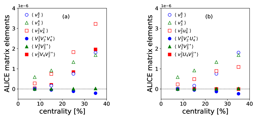
Figure 1: (a) Elements of the matrix $\Sigma$ in Eq. (14) in Pb+Pb collisions at $\sqrt{s}=2.76$ TeV, as a function of centrality percentile. (b) Same matrix with $V_{4}$ replaced with $U_{4}$ everywhere (see text). We introduce the notation $u_{4}\equiv|U_{4}|$.

Figure 1–(a) displays the elements of $\Sigma$ as a function of the centrality percentile. The off-diagonal element $\Sigma_{13}$ is large due to the strong correlation between $v_{2}$ and $v_{4}$. It is instructive to test how the matrix is modified when one writes the third nonlinear term in terms of $U_{4}$ (instead of $V_{4}$), as in Eq. (5). Using Eq. (1), one shows that this is done by transforming the matrix elements according to

$$\Sigma_{13} \to \Sigma_{13}-\chi_{42}\Sigma_{11},$$ (20)

$$\Sigma_{23} \to \Sigma_{23}-\chi_{42}\Sigma_{21},$$ (21)

$$\Sigma_{33} \to \Sigma_{33}-2\chi_{42}\Sigma_{31}+\chi_{42}^{2}\Sigma_{11},$$ (22)

where $\chi_{42}$ is measured by the ALICE collaboration Acharya:2017zfg . The transformed elements are displayed in Fig. 1–(b). When written in terms of $U_{4}$, the off-diagonal elements (full symbols) are much smaller than the diagonal elements (open symbols), which validates the approximations made in previous analyses Acharya:2017zfg where they were neglected. However, they are not compatible with zero. In particular, $\langle U_{4}V_{2}V_{3}^{2*}\rangle$ is negative. It is therefore important to check to what extent the ALICE measurements, carried out under the assumption of negligible off-diagonal terms, are modified when the full pattern of correlations is taken into account.

As a by-product of our analysis, we can test whether the two components in the decomposition of $V_{4}$, Eq. (1), are independent. We have imposed that they are uncorrelated, which is a weaker assumption. If they are independent, it implies in addition that the matrix element $\langle v_{2}^{2}u_{4}^{2}\rangle$ (open squares in Fig.1–(b)) factorizes into the product $\langle v_{2}^{2}\rangle\langle u_{4}^{2}\rangle$. This can be directly tested using ALICE data, as discussed in Appendix A.

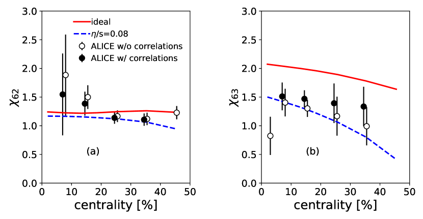
Figure 2: Response coefficients $\chi_{62}$ (a) and $\chi_{63}$ (b) as a function of collision centrality in Pb+Pb collisions at $\sqrt{s}=2.76$ TeV. Open symbols: ALICE analysis Acharya:2017zfg . Full symbols: this analysis, which takes into account the mutual coupling between nonlinear terms. We assume for simplicity that the error is unchanged. Lines are hydrodynamic calculations (see Sec. V), ideal (solid) or viscous (dashed).

IV Nonlinear coefficients of $\boldsymbol{V_{6}}$ from data

We now present our results for the nonlinear response coefficients of $v_{6}$ extracted from experimental data using Eq. (12). The coefficient $\chi_{624}$ has already been calculated in hydrodynamics Qian:2016pau ; Zhao:2017yhj but its experimental value is shown here for the first time. $\chi_{62}$ and $\chi_{63}$ have already been measured by ALICE under the approximation that the nonlinear terms are independent, while our new analysis takes into account the full correlation matrix.

Our results for the coefficients $\chi_{62}$ and $\chi_{63}$ are shown as full symbols in Fig. 2, and we compare them to the previous ALICE results, shown as open symbols. Comparison between the two sets of points shows that mutual correlations between nonlinear terms in Eq. (5) only have small effects. When they are taken into account, however, the centrality dependence of the response coefficient is somewhat flatter. As will be discussed in Sec. V, this generically improves agreement with hydrodynamics. Taking into account the error bars, one cannot exclude that both response coefficients are independent of centrality. Note that, although within error bars, $\chi_{63}$ extracted from the full correlation matrix appears to be systematically larger that the previous ALICE data. This is a signature of the largest non-diagonal term in $\Sigma$, namely, $\langle U_{4}V_{2}(V_{3}^{*})^{2}\rangle$.

Figure 3: Response coefficient $\chi_{624}$ as a function of collision centrality in Pb+Pb collisions at $\sqrt{s}=2.76$ TeV. Symbols denote the coefficient extracted from experimental data, both when the full correlation matrix is taken into account (open symbols), and when correlations are neglected (full symbols). Lines: Results from ideal (solid line) and viscous (dashed line) hydrodynamics.

Figure 3 displays the first experimental result for $\chi_{624}$. It is larger than $\chi_{62}$ and $\chi_{63}$ for all centralities. It also has a stronger centrality dependence, but the large errors prevent any definite conclusion. We estimate these errors by taking into account only the error on the event-plane correlation (second line of Eq. (17)), which is the largest error. If a dedicated analysis of $\chi_{624}$ was carried out, however, the error bar would likely be as small as that on $\chi_{62}$ and $\chi_{63}$. The reason is that a dedicated analysis would measure directly $\langle V_{2}^{*}V_{4}^{*}V_{6}\rangle$, which is linear in $V_{6}$, while we extract it by combining the event-plane correlation and $v_{6}\{2\}$, which are both quadratic in $V_{6}$, and therefore have a larger error. In Fig. 3 (open symbols) we present as well the coefficient extracted from data in absence of mutual correlations between the nonlinear terms. It is given by the following expression

$$\chi_{624}=\frac{\langle V_{6}V_{2}^{*}U_{4}^{*}\rangle}{\langle u_{4}^{2}v_{2}^{2}\rangle},$$ (23)

and it corresponds to the quantity computed in theoretical analyses Qian:2016fpi ; Qian:2017ier ; Zhao:2017yhj . This simplified expression returns a result very close to the full result.

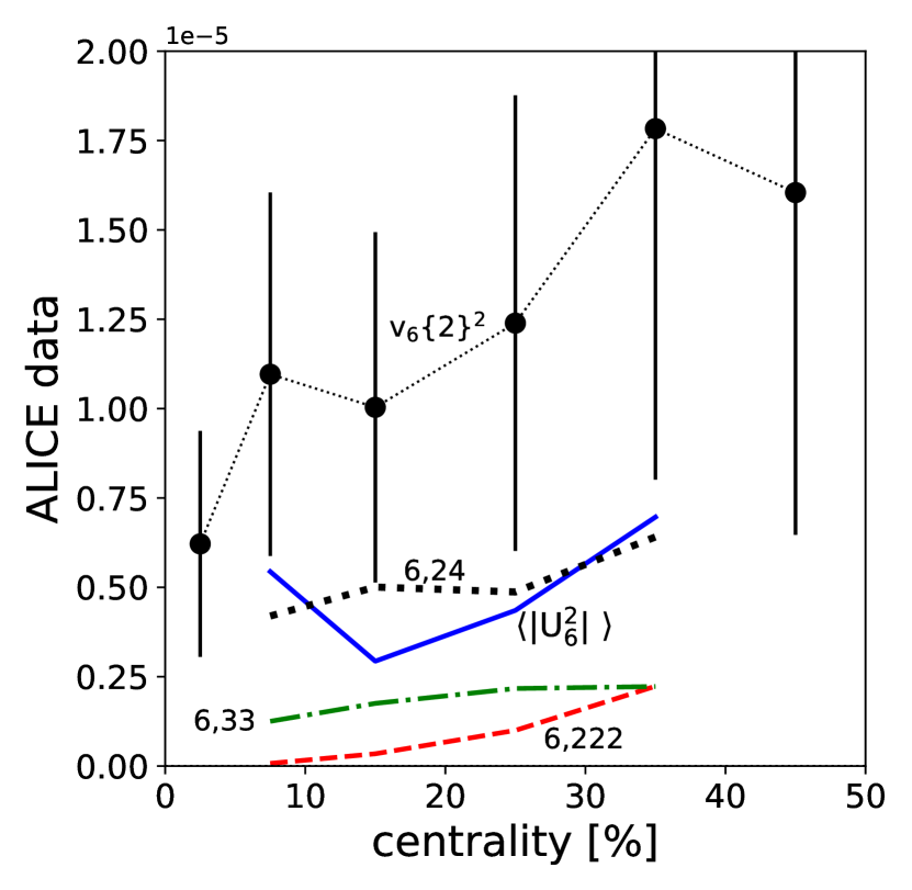
Figure 4: Nonlinear contributions to $\langle|V_{6}|^{2}\rangle$, as given by Eq. (24), extracted from ALICE data. Symbols: $\langle|V_{6}|^{2}\rangle$ Acharya:2017zfg . Solid line: $\langle|U_{6}|^{2}\rangle$. Thick dotted line: $\chi_{624}\langle V_{6}^{*}V_{2}U_{4}\rangle$. Dot-dashed line: $\chi_{63}\langle V_{6}^{*}V_{3}^{2}\rangle$. Dashed line: $\chi_{624}\langle V_{6}^{*}V_{2}^{3}\rangle$.

It is further instructive to compare the magnitudes of the various non-linear contributions to $V_{6}$. In the case of the decomposition (5), Eq. (13) reads:

$$\langle|V_{6}|^{2}\rangle=\langle|U_{6}|^{2}\rangle+\chi_{62}\langle V_{6}^{*}V_{2}^{3}\rangle+\chi_{63}\langle V_{6}^{*}V_{3}^{2}\rangle+\chi_{624}\langle V_{6}^{*}V_{2}U_{4}\rangle.$$ (24)

Figure 4 displays the values of all the terms appearing in this equation as a function of centrality. $\langle|U_{6}|^{2}\rangle$ is calculated as the difference between $v_{6}\{2\}^{2}$ and the sum of the other terms. The largest nonlinear contribution to $v_{6}$ is that due to the coupling with $v_{2}$ and $v_{4}$, while terms proportional to $(v_{2})^{3}$ and $(v_{3})^{2}$ are subleading for all centralities.

V Hydrodynamic calculation

Nonlinear response coefficients are unique probes of hydrodynamic behavior, because they are essentially independent of the initial state Yan:2015jma . The uncertainty on the initial state is the bottleneck in traditional hydro-to-data comparisons Luzum:2008cw , because traditional flow observables such as $v_{2}$ or $v_{3}$ are driven by initial anisotropies in the corresponding harmonics, which are poorly constrained. The dependence on these initial anisotropies cancels in the ratios defining the nonlinear response coefficients. This explains why all nonlinear response coefficients depend weakly on centrality in hydrodynamic calculations Qian:2016fpi ; Zhao:2017yhj . This is in sharp contrast with the steep centrality dependence of $v_{2}$. Two different models of initial conditions with different $v_{2}$ and $v_{3}$ also return the same value for the nonlinear response coefficients. In this Section, we perform hydrodynamic calculations of the nonlinear response coefficients of $v_{6}$, and we compare them to the coefficients previously extracted from experimental data.

Because of the aforementioned weak dependence on initial state, we evaluate these coefficients in a single collision event with a smooth initial density profile. The density profile is constructed by a smooth deformation of a symmetric 2-dimensional Gaussian, following Ref. Teaney:2012ke . If one imprints a small elliptic deformation to the initial profile (a small asymmetry between the width along $x$ and $y$), the subsequent expansion generates all even Fourier harmonics, while odd harmonics (such as $V_{3}$) vanish because of $\phi\to\phi+\pi$ symmetry. In this situation, $V_{4}$ is solely generated by $V_{2}$, so that $U_{4}$ vanishes. Only the first nonlinear term remains in Eq. (5), therefore, $\chi_{62}=V_{6}/(V_{2})^{3}$. Similarly, one evaluates $\chi_{63}$ by imprinting a small triangular deformation to a radially symmetric profile, in which case $\chi_{63}=V_{6}/(V_{3})^{2}$. With this choice of initial conditions, the interpretation of $\chi_{62}$ and $\chi_{63}$ is transparent: they directly quantify the hexagonal flow produced by elliptic flow and triangular flow, respectively.

In the case of $\chi_{624}$, one needs to deform the initial profile in harmonics 2 and 4. We carry out two hydrodynamic calculations, one with an asymmetric Gaussian profile, labeled (A) and one with a small quadrangular deformation (with the same orientation) on top of the asymmetric Gaussian, labeled (B). We compute $V_{2}$, $V_{4}$ and $V_{6}$ at the end of the hydrodynamic evolution for both initial conditions. The initial conditions (A) and (B) differ only in the fourth Fourier harmonic, hence the values of $V_{2}$ are almost identical, $V_{2A}\simeq V_{2B}\equiv V_{2}$. We first evaluate the change of $V_{4}$ induced by the quadrangular deformation, which is denoted by $U_{4}$ in Eq. (1), and given by $U_{4}\equiv V_{4B}-V_{4A}$. Then, the response coefficient $\chi_{624}$ defined by Eq. (5) is given by the increase of $V_{6}$ driven by the quadrangular deformation, i.e.:

$$\chi_{624}\equiv\frac{V_{6B}-V_{6A}}{V_{2}U_{4}}=\frac{V_{6B}-V_{6A}}{V_{2}(V_{4B}-V_{4A})}.$$ (25)

We carry out this calculation for both ideal hydrodynamics and viscous hydrodynamics with $\eta/s=1/4\pi$ Kovtun:2004de . We compute pion spectra at a freeze-out temperature of $T_{f}=130$ MeV. This simple setup is justified by previous studies which have shown Qian:2016fpi that a more elaborate calculation taking into account the full hadron spectrum and strong decays returns almost identical nonlinear response coefficients. The resulting nonlinear response coefficients are plotted as lines in Figs. 2 and 3. Interestingly, the values for $\chi_{63}$ and $\chi_{624}$ are very close to those given by a full event-by-event hydrodynamic calculation Qian:2016fpi , implementing MC Glauber or MC KLN initial conditions. Zhao et al. Zhao:2017yhj find significantly smaller values ($\chi_{63}$ is around 1, $\chi_{624}$ around 2) and do not comment on this difference with previous calculations.

In our hydrodynamic calculation, the centrality enters only through the initial transverse radius, which we estimate in a Glauber model. As the centrality percentile increases, this radius decreases and off-equilibrium effects become larger (earlier freeze out, and larger dissipative corrections both during the hydrodynamic expansion and at freeze out). This explains the mild centrality dependence of nonlinear response coefficients. This mild dependence is a characteristic of hydrodynamic models in general. A steep variation of any nonlinear response coefficient would indicate a failure of the hydrodynamic picture. Experimental results for $\chi_{62}$ and $\chi_{63}$ are so far compatible with hydrodynamics. Our results on $\chi_{624}$, on the other hand, seem not capture the centrality dependence of the extracted experimental values. This underlines the necessity of a dedicated analysis for reducing the error bars on this quantity.

Our results for $\chi_{62}$ and $\chi_{624}$ are mildly affected by adding shear viscosity to the hydrodynamic calculation. Viscosity results in a modest reduction of response coefficients, the effect being largest in peripheral collisions. For $\chi_{63}$, we find a larger dependence on viscosity, and data are only compatible with viscous results. This large depenence is not observed in event-by-event calculations Qian:2016fpi .

VI Extension to higher harmonics

The data-driven analysis carried out in the previous sections show that the assumptions made in the literature about $V_{6}$ are reasonable: The matrix $\Sigma^{(6)}$ is essentially diagonal. In this section we argue, though, that it will be crucial to take into account the full pattern of correlations in harmonics of higher-order, such as $V_{7}$ Tuo:2017ucz , and potentially $V_{8}$.

For heptagonal flow, there are also three leading nonlinear terms:

$$V_{7}=\chi_{723}V_{2}^{2}V_{3}+\chi_{725}V_{2}U_{5}+\chi_{734}V_{3}U_{4}+U_{7}.$$ (26)

Using Eqs. (1) and (3), we rewrite the nonlinear terms as a function of the conventional harmonics $V_{n}$:

$$V_{7} = (\chi_{723}-\chi_{725}\chi_{523}-\chi_{734}\chi_{42})V_{2}^{2}V_{3}$$ (28)

$$+\chi_{725}V_{2}V_{5}+\chi_{734}V_{3}V_{4}+U_{7},$$

which is again of the type (7) with $W_{1}=V_{2}^{2}V_{3}$, $W_{2}=V_{2}V_{5}$, $W_{3}=V_{3}V_{4}$. The correlation matrix (10) is:

$$\Sigma^{(7)}=\begin{pmatrix}\langle v_{2}^{4}v_{3}^{2}\rangle&\langle v_{2}^{2}V_{2}^{*}V_{3}^{*}V_{5}\rangle&\langle v_{3}^{2}V_{2}^{2*}V_{4}\rangle\\ \langle v_{2}^{2}V_{2}V_{3}V_{5}^{*}\rangle&\langle v_{2}^{2}v_{5}^{2}\rangle&\langle V_{5}^{*}V_{2}^{*}V_{3}V_{4}\rangle\\ \langle v_{3}^{2}V_{2}^{2}V_{4}^{*}\rangle&\langle V_{5}V_{2}V_{3}^{*}V_{4}^{*}\rangle&\langle v_{3}^{2}v_{4}^{2}\rangle\end{pmatrix}.$$ (29)

Note that $\Sigma_{23}$ involves four different Fourier harmonics, and is related to a 4-plane correlation Bhalerao:2013ina . Hydrodynamic calculations of $\chi$ coefficients involving $V_{7}$ are already on the market Qian:2016fpi ; Qian:2017ier ; Zhao:2017yhj , and always implicitly assume that the matrix is diagonal. It will be interesting to see if the hydrodynamic results for $\chi_{723}$, $\chi_{725}$ and $\chi_{734}$ are modified once the full correlation structure is taken into account.

For completeness, let us also provide the correlation matrix of $V_{8}$, a coefficient which is likely to be accessible to experimental analyses thank to the massive statistics of data collected in Pb+Pb collisions at LHC2. We decompose $V_{8}$ as follows:

$$V_{8}=\chi_{82}V_{2}^{4}+ \chi_{823}V_{2}V_{3}^{2}+\chi_{824}V_{2}^{2}U_{4}+\chi_{826}V_{2}U_{6}$$

$$+\chi_{835}V_{3}U_{5}+\chi_{84}U_{4}^{2}+U_{8},$$ (30)

which, in terms of the harmonics $V_{n}$, reads

$$V_{8}= \bigl{(}\chi_{82}-\chi_{824}\chi_{42}-\chi_{826}\chi_{62}+$$

$$\hskip 25.0pt+\chi_{826}\chi_{624}\chi_{42}+\chi_{84}\chi_{42}^{2}\bigr{)}V_{2}^{4}$$

$$+\bigl{(}\chi_{823}-\chi_{826}\chi_{63}-\chi_{835}\chi_{523}\bigr{)}V_{2}V_{3}^{2}$$

$$+\bigl{(}\chi_{824}-\chi_{826}\chi_{624}-2\chi_{84}\chi_{42}\bigr{)}V_{2}^{2}V_{4}$$

$$+\chi_{826}V_{2}V_{6}+\chi_{835}V_{3}V_{5}+\chi_{84}V_{4}^{2}+U_{8}.$$ (31)

This leads to the following $6\times 6$ correlation matrix:

$$\Sigma^{(8)}=\begin{pmatrix}\langle v_{2}^{8}\rangle&\langle v_{2}^{2}V_{3}^{2}V_{2}^{3*}\rangle&\langle v_{2}^{4}V_{4}V_{2}^{2*}\rangle&\langle v_{2}^{2}V_{6}V_{2}^{3*}\rangle&\langle V_{5}V_{3}V_{2}^{4*}\rangle&\langle V_{4}^{2}V_{2}^{4*}\rangle\\ {\rm c.c.}&\langle v_{2}^{2}v_{3}^{4}\rangle&\langle v_{2}^{2}V_{2}V_{4}V_{3}^{2*}\rangle&\langle v_{2}^{2}V_{6}V_{3}^{2*}\rangle&\langle v_{3}^{2}V_{5}V_{2}^{*}V_{3}^{*}\rangle&\langle V_{4}^{2}V_{2}^{*}V_{3}^{2*}\rangle\\ {\rm c.c.}&{\rm c.c.}&\langle v_{2}^{4}v_{4}^{2}\rangle&\langle v_{2}^{2}V_{6}V_{2}^{*}V_{4}^{*}\rangle&\langle V_{5}V_{3}V_{2}^{2*}V_{4}^{*}\rangle&\langle v_{4}^{2}V_{4}V_{2}^{2*}\rangle\\ {\rm c.c.}&{\rm c.c.}&{\rm c.c.}&\langle v_{2}^{2}v_{6}^{2}\rangle&\langle V_{5}V_{3}V_{2}^{*}V_{6}^{*}\rangle&\langle V_{4}^{2}V_{2}^{*}V_{6}^{*}\rangle\\ {\rm c.c.}&{\rm c.c.}&{\rm c.c.}&{\rm c.c.}&\langle v_{5}^{2}v_{3}^{2}\rangle&\langle V_{4}^{2}V_{3}^{*}V_{5}^{*}\rangle\\ {\rm c.c.}&{\rm c.c.}&{\rm c.c.}&{\rm c.c.}&{\rm c.c.}&\langle v_{4}^{4}\rangle\end{pmatrix}.$$ (32)

Let us stress once more, then, that the extraction of the nonlinear coefficients in our framework involves only moments which are linear in $V_{8}$, and, therefore, experimentally easier to achieve than typical observables such as $\langle v_{8}^{2}\rangle$.

VII Conclusion

We have proposed a new framework which allows to systematically isolate the various nonlinear contributions to a given higher-order harmonic, and measure the nonlinear coupling coefficients. It can be applied to both experimental data and event-by-event hydrodynamic calculations. The main improvement over previous analyses is that we take into account the mutual correlations between nonlinear contributions. We have applied this new framework to $V_{6}$ using existing data. When mutual correlations are properly taken into account, the centrality dependence of the response coefficients $\chi_{62}$ and $\chi_{63}$ becomes somewhat flatter, thus improving agreement with hydrodynamic predictions. We have provided the first experimental determination of the coefficient $\chi_{624}$ coupling $v_{6}$ to $v_{2}$ and $v_{4}$. It is in fair agreement with hydrodynamic predictions, though with large error bars. The corresponding nonlinear term is the largest of the three nonlinear contributions to $v_{6}$. With the advent of large statistics Pb+Pb LHC2 data, we expect that this new framework will enable detailed analyses of higher-order flow coefficients, which will provide precision tests of hydrodynamic behavior.

Appendix A Correlation between $\boldsymbol{u_{4}^{2}}$ and $\boldsymbol{v_{2}^{2}}$

In the definition of quadrangular flow in Eq. (1), one chooses $U_{4}$ and $V_{2}^{2}$ to be uncorrelated by construction, i.e.,

$$\langle U_{4}^{*}V_{2}^{2}\rangle=0.$$ (33)

In the literature Qian:2016fpi ; Giacalone:2016afq ; Qian:2017ier ; Zhao:2017yhj , though, this has always been supplemented by the following assumption:

$$\langle u_{4}^{2}v_{2}^{2}\rangle=\langle u_{4}^{2}\rangle\langle v_{2}^{2}\rangle,$$ (34)

which implies statistical independence between the two terms. Statistical independence is a much stronger constraint than just requiring the two terms to be uncorrelated.

In this appendix we check the validity of Eq. (34) using experimental data. The equality can be conveniently tested by introducing the following normalized symmetric cumulant Bilandzic:2013kga ; ALICE:2016kpq

$$sc(4,2)_{U}=\frac{\langle u_{4}^{2}v_{2}^{2}\rangle-\langle u_{4}^{2}\rangle\langle v_{2}^{2}\rangle}{\langle u_{4}^{2}\rangle\langle v_{2}^{2}\rangle},$$ (35)

which vanishes if $u_{4}^{2}$ and $v_{2}^{2}$ are independent. All the terms appearing in the definition of $sc(4,2)_{U}$ are available from ALICE data. The quantity $\langle u_{4}^{2}\rangle$ was recently measured Acharya:2017zfg , and $\langle u_{4}^{2}v_{2}^{2}\rangle$ is given by $\Sigma_{33}$ in Eq. (22). The resulting cumulant is displayed as black circles in Fig. 5.

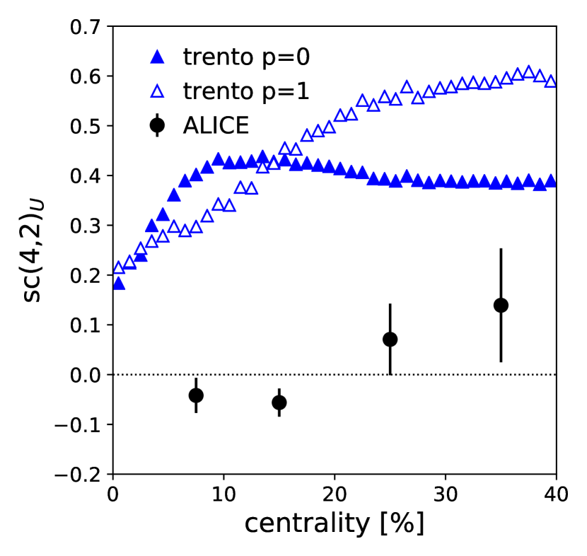
Figure 5: Circles: $sc(4,2)_{U}$, as given by Eq. (35), from ALICE data. Triangles: T$\mathrel{\raisebox{-2.1pt}{R}}$ENTo calculations for $sc(4,2)_{\varepsilon}$, Eq. (36).

This result illustrates that $sc(4,2)_{U}$ is indeed small in magnitude, so that Eq. (34) is a good approximation, although error bars, driven by the uncertainty on SC(4,2), are large in non-central collisions.

We ask now whether this quantity carries any useful information about the initial state of the hydrodynamic evolution. In heavy-ion collisions, elliptic flow is to a good approximation proportional to the second eccentricity harmonic of the initial state, $\varepsilon_{2}$ Teaney:2010vd . As for the fourth harmonic, it is often argued that $U_{4}$ may scale linearly with the fourth cumulant eccentricity of the initial medium Qian:2017ier , which is customarily taken from Ref. Teaney:2012ke :

$$\mathcal{C}_{4}=\mathcal{E}_{4}+3\frac{\langle r^{2}\rangle^{2}}{\langle r\rangle^{4}}\mathcal{E}_{2}^{2},$$

where $\mathcal{E}_{n}$ corresponds to the moment-defined eccentricity harmonic of order $n$ Teaney:2010vd .

Now, dubbing $c_{4}=|\mathcal{C}_{4}|$, if $\mathcal{C}_{4}$ scales linearly with $U_{4}$, then the following quantity

$$sc(4,2)_{\varepsilon}=\frac{\langle c_{4}^{2}\varepsilon_{2}^{2}\rangle-\langle c_{4}^{2}\rangle\langle\varepsilon_{2}^{2}\rangle}{\langle c_{4}^{2}\rangle\langle\varepsilon_{2}^{2}\rangle}$$ (36)

should match to a good extent $sc(4,2)_{U}$ observed in ALICE data, at least in central collisions where $U_{4}$ dominates. To check this, we compute $sc(4,2)_{\varepsilon}$ from initial-state simulations of Pb+Pb collisions at $~{}\sqrt[]{s}=2.76$ TeV. We perform this by employing two different setups of the T$\mathrel{\raisebox{-2.1pt}{R}}$ENTo model of initial conditions Moreland:2014oya . We use T$\mathrel{\raisebox{-2.1pt}{R}}$ENTo with $p=1$, corresponding to a Glauber Monte Carlo model, and $p=0$, which provides eccentricities in agreement with models including high-energy QCD effects, such as EKRT or IP-Glasma Moreland:2014oya . Our results from the initial state models are shown in Fig. 5. The correlation is moderate and positive already at 0% centrality, therefore, we do not find agreement between the model calculation and experimental data. Therefore, typical models of initial conditions do not suggest a linear correlation between $\mathcal{C}_{4}$ and $U_{4}$, in contradiction, then, with the finding of hydrodynamic calculations Qian:2017ier . We remark, though, that this failure may be equally due to either the fact that the fourth-order initial-state anisotropy is not correctly quantified by $\mathcal{C}_{4}$, or that $\mathcal{C}_{4}$ is not captured by the initial-state models, or both.

References

- (1) U. Heinz and R. Snellings, Ann. Rev. Nucl. Part. Sci. 63, 123 (2013) doi:10.1146/annurev-nucl-102212-170540 [arXiv:1301.2826 [nucl-th]].
- (2) G. Aad et al. [ATLAS Collaboration], Phys. Rev. C 86, 014907 (2012) doi:10.1103/PhysRevC.86.014907 [arXiv:1203.3087 [hep-ex]].
- (3) S. Chatrchyan et al. [CMS Collaboration], Phys. Rev. C 89, no. 4, 044906 (2014) doi:10.1103/PhysRevC.89.044906 [arXiv:1310.8651 [nucl-ex]].
- (4) S. Acharya et al. [ALICE Collaboration], Phys. Lett. B 773, 68 (2017) doi:10.1016/j.physletb.2017.07.060 [arXiv:1705.04377 [nucl-ex]].
- (5) S. Tuo [CMS Collaboration], Nucl. Phys. A 967, 381 (2017). doi:10.1016/j.nuclphysa.2017.05.064
- (6) M. Luzum and J. Y. Ollitrault, Nucl. Phys. A 904-905, 377c (2013) doi:10.1016/j.nuclphysa.2013.02.028 [arXiv:1210.6010 [nucl-th]].
- (7) S. Chatrchyan et al. [CMS Collaboration], JHEP 1402, 088 (2014) doi:10.1007/JHEP02(2014)088 [arXiv:1312.1845 [nucl-ex]].
- (8) F. G. Gardim, F. Grassi, M. Luzum and J. Y. Ollitrault, Phys. Rev. C 85, 024908 (2012) doi:10.1103/PhysRevC.85.024908 [arXiv:1111.6538 [nucl-th]].
- (9) L. Yan and J. Y. Ollitrault, Phys. Lett. B 744, 82 (2015) doi:10.1016/j.physletb.2015.03.040 [arXiv:1502.02502 [nucl-th]].
- (10) W. Zhao, H. j. Xu and H. Song, Eur. Phys. J. C 77, no. 9, 645 (2017) doi:10.1140/epjc/s10052-017-5186-x [arXiv:1703.10792 [nucl-th]].
- (11) N. Borghini and J. Y. Ollitrault, Phys. Lett. B 642, 227 (2006) doi:10.1016/j.physletb.2006.09.062 [nucl-th/0506045].
- (12) D. Teaney and L. Yan, Phys. Rev. C 86, 044908 (2012) doi:10.1103/PhysRevC.86.044908 [arXiv:1206.1905 [nucl-th]].
- (13) J. Qian, U. W. Heinz and J. Liu, Phys. Rev. C 93, no. 6, 064901 (2016) doi:10.1103/PhysRevC.93.064901 [arXiv:1602.02813 [nucl-th]].
- (14) L. V. Bravina et al., Phys. Rev. C 89, no. 2, 024909 (2014) doi:10.1103/PhysRevC.89.024909 [arXiv:1311.0747 [hep-ph]].
- (15) J. Qian, U. Heinz, R. He and L. Huo, Phys. Rev. C 95, no. 5, 054908 (2017) doi:10.1103/PhysRevC.95.054908 [arXiv:1703.04077 [nucl-th]].
- (16) P. Liu and R. A. Lacey, arXiv:1802.06595 [nucl-ex].
- (17) G. Aad et al. [ATLAS Collaboration], Phys. Rev. C 90, no. 2, 024905 (2014) doi:10.1103/PhysRevC.90.024905 [arXiv:1403.0489 [hep-ex]].
- (18) R. S. Bhalerao, J. Y. Ollitrault and S. Pal, Phys. Lett. B 742, 94 (2015) doi:10.1016/j.physletb.2015.01.019 [arXiv:1411.5160 [nucl-th]].
- (19) F. Cooper and G. Frye, Phys. Rev. D 10, 186 (1974). doi:10.1103/PhysRevD.10.186
- (20) D. Teaney, Phys. Rev. C 68, 034913 (2003) doi:10.1103/PhysRevC.68.034913 [nucl-th/0301099].
- (21) R. S. Bhalerao, M. Luzum and J. Y. Ollitrault, Phys. Rev. C 84, 034910 (2011) doi:10.1103/PhysRevC.84.034910 [arXiv:1104.4740 [nucl-th]].
- (22) K. Fukushima, D. E. Kharzeev and H. J. Warringa, Phys. Rev. D 78, 074033 (2008) doi:10.1103/PhysRevD.78.074033 [arXiv:0808.3382 [hep-ph]].
- (23) S. Voloshin and Y. Zhang, Z. Phys. C 70, 665 (1996) doi:10.1007/s002880050141 [hep-ph/9407282].
- (24) R. S. Bhalerao, J. Y. Ollitrault and S. Pal, Phys. Rev. C 88, 024909 (2013) doi:10.1103/PhysRevC.88.024909 [arXiv:1307.0980 [nucl-th]].
- (25) K. Aamodt et al. [ALICE Collaboration], Phys. Rev. Lett. 107, 032301 (2011) doi:10.1103/PhysRevLett.107.032301 [arXiv:1105.3865 [nucl-ex]].
- (26) S. Acharya et al. [ALICE Collaboration], Phys. Rev. C 97, no. 2, 024906 (2018) doi:10.1103/PhysRevC.97.024906 [arXiv:1709.01127 [nucl-ex]].
- (27) J. Adam et al. [ALICE Collaboration], Phys. Rev. Lett. 117, 182301 (2016) doi:10.1103/PhysRevLett.117.182301 [arXiv:1604.07663 [nucl-ex]].
- (28) J. Qian and U. Heinz, Phys. Rev. C 94, no. 2, 024910 (2016) doi:10.1103/PhysRevC.94.024910 [arXiv:1607.01732 [nucl-th]].
- (29) M. Luzum and P. Romatschke, Phys. Rev. C 78, 034915 (2008) Erratum: [Phys. Rev. C 79, 039903 (2009)] doi:10.1103/PhysRevC.78.034915, 10.1103/PhysRevC.79.039903 [arXiv:0804.4015 [nucl-th]].
- (30) P. Kovtun, D. T. Son and A. O. Starinets, Phys. Rev. Lett. 94, 111601 (2005) doi:10.1103/PhysRevLett.94.111601 [hep-th/0405231].
- (31) G. Giacalone, L. Yan, J. Noronha-Hostler and J. Y. Ollitrault, Phys. Rev. C 94, no. 1, 014906 (2016) doi:10.1103/PhysRevC.94.014906 [arXiv:1605.08303 [nucl-th]].
- (32) A. Bilandzic, C. H. Christensen, K. Gulbrandsen, A. Hansen and Y. Zhou, Phys. Rev. C 89, no. 6, 064904 (2014) doi:10.1103/PhysRevC.89.064904 [arXiv:1312.3572 [nucl-ex]].
- (33) D. Teaney and L. Yan, Phys. Rev. C 83, 064904 (2011) doi:10.1103/PhysRevC.83.064904 [arXiv:1010.1876 [nucl-th]].
- (34) J. S. Moreland, J. E. Bernhard and S. A. Bass, Phys. Rev. C 92, no. 1, 011901 (2015) doi:10.1103/PhysRevC.92.011901 [arXiv:1412.4708 [nucl-th]].