Self-gravitating envelope solitons in astrophysical compact objects

Abstract

The propagation of ion-acoustic waves (IAWs) in a collisionless unmagnetized self-gravitating degenerate quantum plasma system (SG-DQPS) has been studied theoretically for the first time. A nonlinear Schrödinger equation is derived by using the reductive perturbation method to study the nonlinear dynamics of the IAWs in the SG-DQPS. It is found that for $k_{c}>k$ ($k_{c}<k$) (where $k_{c}$ is critical value of the propagation constant $k$ which determines the stable and unstable region of IAWs) the IAWs are modulationally unstable (stable), and that $k_{c}$ depends only on the ratio of the electron number density to light ion number density. It is also observed that the self-gravitating bright envelope solitons are modulationally stable. The results obtained from our present investigation are useful for understanding the nonlinear propagation of the IAWs in astrophysical compact objects like white dwarfs and neutron stars.

I Introduction

Recently, the self-gravity of degenerate quantum plasma (DQP) is the cornerstone among the plasma physicists to understand the basic features of the astrophysical compact objects (viz. white dwarf, neutron stars Chandrasekhar1931 ; Fowler1994 ; Shapiro1983 ; Koester1990 ; Koester2002 ; Shukla2011 ; Zaman2017 ) as well as in laboratory environments (viz. solid density plasmas Drake2009 ; Drake2010 , laser produced plasmas formed from sold targets irradiating by intense laser Glenzer2009 , ultra-cold plasmas Fletcher2006 ; Killian2006 , etc.). The self-gravitating DQP system (SG-DQPS) has a large number of ultra-relativistic or non-relativistic degenerate species (order of $10^{30}cm^{-3}$ in white dwarfs, and order of $10^{36}cm^{-3}$ even more in neutron stars Shapiro1983 ; Koester1990 ; Koester2002 ) and extremely low temperature which exhibits unique collective behaviours from others plasma system. The basic constituents of the SG-DQPS (viz. white dwarf, neutron stars) are degenerate inertialess electron species Chandrasekhar1931 ; Fowler1994 ; Shapiro1983 ; Koester1990 ; Koester2002 , degenerate inertial light ion species (viz.${\rm~{}^{1}_{1}H}$ Fletcher2006 ; Killian2006 , ${\rm~{}^{4}_{2}He}$ Chandrasekhar1931 ; Fowler1994 , and ${\rm~{}^{12}_{~{}6}C}$ Koester1990 ; Koester2002 ), and heavy ion species (viz.${\rm~{}^{56}_{26}Fe}$ Vanderburg2015 , ${\rm~{}^{85}_{37}Rb}$ Witze2014 , and ${\rm~{}^{96}_{42}Mo}$ Witze2014 ).

The dynamics of the SG-DQPS is governed by the quantum mechanics because of the de Broglie wavelength of particles is comparable to the inter-particle distance in SG-DQPS Shapiro1983 ; Koester1990 . According to the Heisenberg s uncertainty principle, in quantum realm, the exact position and momentum of a particle cannot be determined simultaneously, and mathematically it can be expressed as $\Delta x\Delta p\geq\hbar/2$ (where $\Delta x$ is the uncertainty in position of the particle and $\Delta p$ is the uncertainty in momentum of the same particle, and $\hbar$ is the reduced Planck constant). In SG-DQPS, the position (momentum) of the plasma species is well (not well) defined and these confined plasma species with uncertain momentum exerts a pressure on the surrounding medium. Chandrasekhar more than 80 years ago defined this exert pressure as degenerate pressure and mathematically it can be expressed as Chandrasekhar1931 ; Fowler1994

$$P_{j}=K_{j}N_{j}^{\gamma},~{}~{}~{}~{}~{}K_{j}\simeq\frac{3}{5}\frac{\pi\hbar^{2}}{m_{j}},$$ (1)

where $j=e$ for the electron species, $j=l$ ($h$) for light (heavy) ion species, $K_{j}$ is the proportional constant, $\gamma$ is a relativistic factor and $\gamma=5/4$ ($5/3$) stands for ultra-relativistic (non-relativistic) limit, and $m_{j}$ is the mass of the plasma species. The degenerate pressure of the SG-DQPS is dependent (independent) on the number density and mass (temperature) of the plasma species. The mass of the plasma species generates a strong gravitational field which provides the inward pull to compress the plasma system, but this inward pull is counter-balanced by the outward degenerate pressure.

The amplitude of the ion-acoustic waves (IAWs) is appeared to modulation due to wave-particle interaction, the nonlinear self-interaction of the carrier wave modes, interaction between low and high frequency modes Chowdhury2017a ; Sultana2011 ). The modulational instability (MI) and generation of the envelope solitons in any nonlinear and dispersive medium are governed by the the nonlinear Schrödinger (NLS) equation. Recently, a large number of authors have studied the nonlinear wave propagation in SG-DQPS. Asaduzzaman et al. Asaduzzaman2017 have investigated the nonlinear propagation of self-gravitational perturbation mode in a super dense DQP medium. Mamun Mamun2017 analyzed shock structures in a self-gravitating, multi-component DQP and found that the height and thickness of the shock structures are totally dependent on the dissipative and nonlinear coefficients. Chowdhury et al. Chowdhury2018 have reported that the MI of nucleus-acoustic waves (NAWs) in a DQP system and found that the MI growth rate of the unstable NAWs is significantly modified by the number density of nucleus species. Islam et al. Islam2017 have studied envelope solitons in three component DQP. However to the best of our knowledge, no attempt has been made to study MI of the IAWs in SG-DQPS. Therefore, in the present work, we will derive a NLS equation by employing reductive perturbation method to study the MI and formation of the envelope solitons in a SG-DQPS (containing inertialess degenerate electron species, inertial degenerate light as well as heavy ion species).

The manuscript is organized as follows: The basic governing equations of our plasma model is presented in Sec. II. Derivation of a NLS equation using reductive perturbation technique is presented in Sec. III. The stability of the IAWs and envelope solitons are examined in Sec. IV. A brief discussion is provided in Sec. V.

II Governing Equations

We consider a SG-DQPS comprising of inertialess degenerate electron species $e$, inertial degenerate light ion species $l$, and heavy ion species $h$, respectively. The detail information about light and heavy nuclei is presented in Table 1. The nonlinear dynamics of such a SG-DQPS is governed by the following equations

$$\frac{\partial P_{e}}{\partial X}=-{m_{e}}{N_{e}}\frac{\partial\tilde{\psi}}{\partial X},$$ (2)

$$\frac{\partial N_{l}}{\partial T}+\frac{\partial}{\partial X}(N_{l}U_{l})=0,$$ (3)

$$\frac{\partial U_{l}}{\partial T}+U_{l}\frac{\partial U_{l}}{\partial X}=-\frac{\partial\tilde{\psi}}{\partial X}-\frac{1}{m_{l}N_{l}}\frac{\partial P_{l}}{\partial X},$$ (4)

$$\frac{\partial^{2}\tilde{\psi}}{\partial X^{2}}=4\pi G~{}[m_{e}N_{e}+m_{l}N_{l}+m_{h}N_{h}],$$ (5)

where $T(X)$ is the time (space) variable; $P_{e}$ ($P_{l}$) is the degenerate pressure associated with degenerate electrons (light ions); $m_{e}$, $m_{l}$, and $m_{h}$ is the mass of electrons, light, and heavy ions, respectively; $N_{e}$, $N_{l}$, and $N_{h}$ is, respectively, the number densities of the electrons, light, and heavy ions; $U_{l}$ is the light ion fluid speed; $\tilde{\psi}$ is the self-gravitational potential; $G$ is the universal gravitational constant. Now, the quasi-neutrality condition at equilibrium can be expressed as

$$N_{e}=Z_{l}N_{l}+Z_{h}N_{h},$$ (6)

where $Z_{l}$ ($Z_{h}$) is the charge state of a light (heavy) ion. For the purposes of simplicity, we have considered the continuity and momentum balance equation for the inertial light ion species $l$. Now, introducing normalized variables, specifically, $x=X/L_{q}$, $t=T/\omega_{jl}$, $n_{l}=N_{l}/n_{l0}$, $u_{l}=U_{l}/C_{q}$, $\tilde{\psi}=C_{q}^{2}\psi$, [where $C_{q}=\sqrt{\pi}\hbar n_{e0}^{1/3}/m_{l}$, $\omega_{jl}=4\pi Gm_{l}n_{lo}$, $L_{q}=C_{q}/\omega_{jl}$; $n_{l0}$ ($n_{e0}$) is the equilibrium number densities of light ion species (electrons); $\psi$ is the dimensionless self-gravitational potential. After normalization, Eqs. (2)$-$(5) appear in the following form

$$\frac{\partial\psi}{\partial x}=-\frac{3}{2}\alpha\frac{\partial n_{e}^{2/3}}{\partial x},$$ (7)

$$\frac{\partial n_{l}}{\partial t}+\frac{\partial}{\partial x}(n_{l}u_{l})=0,$$ (8)

$$\frac{\partial u_{l}}{\partial t}+u_{l}\frac{\partial u_{l}}{\partial x}=-\frac{\partial\psi}{\partial x}-\beta\frac{\partial n_{l}^{2/3}}{\partial x},$$ (9)

$$\frac{\partial^{2}\psi}{\partial x^{2}}=\gamma_{e}(n_{e}-1)-\gamma_{l}(n_{l}-1),$$ (10)

where $\alpha=m_{l}/m_{e}$, $\beta=(3/2)\mu^{-2/3}$, $\mu=n_{e0}/n_{l0}$, $\gamma_{e}=\mu(1/\alpha+\gamma/Z_{l})$, $\gamma_{l}=\gamma-1$; $\gamma=Z_{l}m_{h}/Z_{h}m_{l}$ (which is larger than 1 for any set of light and heavy ion species). In $\gamma_{e}$, $1/\alpha\ll\gamma/Z_{l}$ (where $1/\alpha$ varies from $\sim 10^{-4}$ to $\sim 10^{-3}$, and $\gamma/Z_{l}$ varies from $\sim 0.1$ to $\sim 2.0$), so $1/\alpha$ is negligible compared to $\gamma/Z_{l}$, and can be written as $\gamma_{e}\simeq\mu\gamma/Z_{l}$. For inertialess degenerate electron species, the expression for the number density is

$$n_{e}=\left[1-\frac{2\psi}{3\alpha^{2}}\right]^{\frac{3}{2}}$$

$$=1-\frac{1}{\alpha^{2}}\psi+\frac{1}{6\alpha^{4}}\psi^{2}+\frac{1}{54\alpha^{6}}\psi^{3}+\cdot\cdot\cdot\cdot.$$ (11)

Now, by substituting Eq. (11) into Eq. (10), and expanding up to third order in $\psi$, we get

$$\frac{\partial^{2}\psi}{\partial x^{2}}-\gamma_{l}+\gamma_{l}n_{l}=\gamma_{1}\psi+\gamma_{2}\psi^{2}+\gamma_{3}\psi^{3}+\cdot\cdot\cdot\cdot,$$ (12)

where $\gamma_{1}=-\gamma_{e}/\alpha^{2}$, $\gamma_{2}=\gamma_{e}/6\alpha^{4}$, and $\gamma_{3}=\gamma_{e}/54\alpha^{6}$. We note that the terms on the right hand side of Eq. (12) is the contribution of electron.

Table 1: The values of $\gamma$ when ${\rm~{}^{1}_{1}H}$ Fletcher2006 ; Killian2006 , ${\rm~{}^{4}_{2}He}$ Chandrasekhar1931 ; Fowler1994 , and ${\rm~{}^{12}_{~{}6}C}$ Koester1990 ; Koester2002 are considered as the light ion species, and ${\rm~{}^{56}_{26}Fe}$ Vanderburg2015 , ${\rm~{}^{85}_{37}Rb}$ Witze2014 , and ${\rm~{}^{96}_{42}Mo}$ Witze2014 are considered as the heavy ion species.

Light ion	Heavy ion	${\bf\gamma}$
	${\rm~{}^{56}_{26}Fe}$ Vanderburg2015	2.16
${\rm~{}~{}~{}~{}~{}~{}^{1}_{1}H}$ Fletcher2006 ; Killian2006	${\rm~{}^{85}_{37}Rb}$ Witze2014	2.30
	${\rm~{}^{96}_{42}Mo}$ Witze2014	2.28
	${\rm~{}^{56}_{26}Fe}$ Vanderburg2015	1.08
${\rm~{}~{}~{}~{}~{}~{}^{4}_{2}He}$ Chandrasekhar1931 ; Fowler1994	${\rm~{}^{85}_{37}Rb}$ Witze2014	1.15
	${\rm~{}^{96}_{42}Mo}$ Witze2014	1.14
	${\rm~{}^{56}_{26}Fe}$ Vanderburg2015	1.08
${\rm~{}~{}~{}~{}~{}~{}^{12}_{~{}6}C}$ Koester1990 ; Koester2002	${\rm~{}^{85}_{37}Rb}$ Witze2014	1.15
	${\rm~{}^{96}_{42}Mo}$ Witze2014	1.14

III Derivation of the NLS Equation

In order to demonstrate the MI and the basic features of IAWs in a SG-DQPS, we employ the standard reductive perturbation Taniuti1969 ; Chowdhury2017b method in which independent variables are stretched as

$$\left.\begin{array}[]{l}\xi=\epsilon(x-v_{g}t),\\ \tau=\epsilon^{2}t,\end{array}\right\}$$ (13)

hence, we have

$$\frac{\partial}{\partial t}\rightarrow\frac{\partial}{\partial t}-\epsilon v_{g}\frac{\partial}{\partial\xi}+\epsilon^{2}\frac{\partial}{\partial\tau},$$ (14)

$$\frac{\partial}{\partial x}\rightarrow\frac{\partial}{\partial x}+\epsilon\frac{\partial}{\partial\xi},$$ (15)

where $\epsilon$ is a small parameter and $v_{g}$ is the real variable interpreted as the group velocity. Furthermore, the dependent variables $n_{l}$, $u_{l}$, and $\psi$ can be expanded in power series of $\epsilon$ as

$$n_{l}=1+\sum_{m=1}^{\infty}\epsilon^{(m)}\sum_{l^{\prime}=-\infty}^{\infty}n_{ll^{\prime}}^{(m)}(\xi,\tau)~{}\mbox{exp}[il^{\prime}\Upsilon],$$ (16)

$$u_{l}=\sum_{m=1}^{\infty}\epsilon^{(m)}\sum_{l^{\prime}=-\infty}^{\infty}u_{ll^{\prime}}^{(m)}(\xi,\tau)~{}\mbox{exp}[il^{\prime}\Upsilon],$$ (17)

$$\psi=\sum_{m=1}^{\infty}\epsilon^{(m)}\sum_{l^{\prime}=-\infty}^{\infty}\psi_{l^{\prime}}^{(m)}(\xi,\tau)~{}\mbox{exp}[il^{\prime}\Upsilon],$$ (18)

where $\Upsilon=(kx-\omega t)$ and $\omega$ ($k$) corresponds to the angular frequency (wave number) of the carrier waves, respectively. Now, by replacing the Eqs. (13)$-$(18) into Eqs. (8), (9), and (12), and collecting all terms of similar power of $\epsilon$, the first order ($m=1$ with $l^{\prime}=1$) reduced equations can be represented as

$$n_{l1}^{(1)}=\frac{k^{2}}{S}\psi_{1}^{(1)},$$ (19)

$$u_{l1}^{(1)}=\frac{k\omega}{S}\psi_{1}^{(1)},$$ (20)

where $S=\omega^{2}-\beta_{1}k^{2}$ and $\beta_{1}=2\beta/3$. The linear dispersion relation can be obtained from the first-order equations in the form

$$\omega^{2}=\frac{\gamma_{l}k^{2}}{k^{2}+\gamma_{1}}+\beta_{1}k^{2}.$$ (21)

The dispersion properties of IAWs for different values of $\mu$ is depicted in Fig. 2 and it may deduce that (a) the value of $\omega$ exponentially decreases with the increase of $k$; (b) on the other hand, the value of $\omega$ increases (decreases) with $n_{e0}$ ($n_{l0}$).

Figure 1: The variation of $\omega$ with $k$ for different values of $\mu$; along with $\alpha=3.67\times 10^{3}$, $\gamma=2.16$, and $\gamma/Z_{l}=0.5$.

Figure 2: The variation of $P/Q$ with $k$ for different values of $\mu$; along with $\alpha=3.67\times 10^{3}$, $\gamma=2.16$, and $\gamma/Z_{l}=0.5$.

Next, the second-order ($m=2$ with $l^{\prime}=1$) reduced equations are given by

$$n_{l1}^{(2)}=\frac{k^{2}}{S}\psi_{1}^{(2)}+\frac{2i\omega k(v_{g}k-\omega)}{S^{2}}\frac{\partial\psi_{1}^{(1)}}{\partial\xi},$$ (22)

$$u_{l1}^{(2)}=\frac{k\omega}{S}\psi_{1}^{(2)}+\frac{i(\beta_{1}k^{2}+\omega^{2})(v_{g}k-\omega)}{S^{2}}\frac{\partial\psi_{1}^{(1)}}{\partial\xi},$$ (23)

with the compatibility condition

$$v_{g}=\frac{\partial\omega}{\partial k}=\frac{\gamma_{l}\omega^{2}-(\omega^{2}-\beta_{1}k^{2})^{2}}{\gamma_{l}k\omega}.$$ (24)

The amplitude of the second-order harmonics is found to be proportional to $|\psi_{1}^{(1)}|^{2}$

$$\left.\begin{array}[]{l}n_{l2}^{(2)}=C_{1}|\psi_{1}^{(1)}|^{2},~{}~{}~{}~{}~{}~{}~{}~{}~{}n_{l0}^{(2)}=C_{4}|\psi_{1}^{(1)}|^{2},\\ u_{l2}^{(2)}=C_{2}|\psi_{1}^{(1)}|^{2},~{}~{}~{}~{}~{}~{}~{}~{}~{}u_{l0}^{(2)}=C_{5}|\psi_{1}^{(1)}|^{2},\\ \psi_{2}^{(2)}=C_{3}|\psi_{1}^{(1)}|^{2},~{}~{}~{}~{}~{}~{}~{}~{}~{}\psi_{0}^{(2)}=C_{6}|\psi_{1}^{(1)}|^{2},\\ \end{array}\right\}$$ (25)

where

$$C_{1}=\frac{3\omega^{2}k^{4}+2C_{3}k^{2}S^{2}}{2S^{2}},$$

$$C_{2}=\frac{C_{1}\omega S^{2}-\omega k^{4}}{kS^{2}},$$

$$C_{3}=\frac{3\gamma_{l}\omega^{2}k^{4}-2\gamma_{2}S^{3}}{2S^{3}(4k^{2}+\gamma_{1})-2\gamma_{l}k^{2}S^{2}},$$

$$C_{4}=\frac{2\omega v_{g}k^{3}-\beta_{2}k^{4}+k^{2}\omega^{2}+C_{6}S^{2}}{S^{2}(v_{g}^{2}-\beta_{1})},$$

$$C_{5}=\frac{C_{4}v_{g}S^{2}-2\omega k^{3}}{S^{2}},~{}~{}\beta_{2}=\frac{\beta}{9}$$

$$C_{6}=\frac{\gamma_{l}(2\omega v_{g}k^{3}-\beta_{2}k^{4}+k^{2}\omega^{2})-2\gamma_{2}S^{2}(v_{g}^{2}-\beta_{1})}{\gamma_{1}S^{2}(v_{g}^{2}-\beta_{1})-\gamma_{l}S^{2}}.$$

Finally, the third harmonic modes ($m=3$ with $l^{\prime}=1$) provide a set of equations and after some mathematical calculation these equations reduce [with the help of Eqs. (19)$-$(25)] to the following NLS equation:

$$i\frac{\partial\Phi}{\partial\tau}+P\frac{\partial^{2}\Phi}{\partial\xi^{2}}+Q|\Phi|^{2}\Phi=0,$$ (26)

where $\Phi=\psi_{1}^{(1)}$ for simplicity. The dispersion coefficient $P$ and the nonlinear coefficient $Q$ are given by

$$P=\frac{v_{g}\beta_{1}^{2}k^{5}+4\beta_{1}k^{2}\omega^{3}+2\beta_{1}v_{g}\omega^{2}k^{3}-F_{1}}{2\gamma_{l}k^{2}\omega^{2}},$$ (27)

$$Q=\frac{1}{2\gamma_{l}\omega k^{2}S^{2}}\left[2\gamma_{2}(C_{3}+C_{6})S^{4}+2\gamma_{3}S^{4}-F_{2}\right],$$ (28)

where $F_{1}=3v_{g}k\omega^{4}+4\omega\beta_{1}^{2}k^{4}$, $F_{2}=\gamma_{l}k^{2}\omega^{2}S^{2}(C_{1}+C_{4})+2\gamma_{l}\omega S^{2}k^{3}(C_{2}+C_{5})+\gamma_{l}\beta_{3}k^{8}$, and $\beta_{3}=4\beta/81$.

IV MI and envelope solitons

The MI of IAWs can be studied by considering the harmonic modulated amplitude solution of Eq. (26) of the form $\Phi=\hat{\Phi}e^{i\,Q|\hat{\Phi}|^{2}\tau}+c.~{}c.$ (c. c. being the complex conjugate), where perturbed amplitudes are $\hat{\Phi}=\hat{\Phi}_{0}+\epsilon\hat{\Phi}_{1}$ and $\hat{\Phi}_{1}=\hat{\Phi}_{1,0}\exp[i(\tilde{k}\xi-\tilde{\omega}\tau)]+c.~{}c$ (here, the perturbed wave number $\tilde{k}$ and the frequency $\tilde{\omega}$ are different from $k$ and $\omega$). Hence, the nonlinear dispersion relation for the amplitude modulation obtained by substituting these values in Eq. (26) can be written as Sultana2011 ; Schamel2002 ; Chowdhury2018 ; Kourakis2005 ; Fedele2002

$${\tilde{\omega}^{2}}=P^{2}{\tilde{k}^{2}}\left({\tilde{k}^{2}}-\frac{2{|\hat{\Phi}_{o}|^{2}}}{P/Q}\right).$$ (29)

It is apparent from Eq. (29) that the IAWs will be modulationally stable (unstable) for the range of values of $\tilde{k}$ in which $P/Q$ is negative (positive), such as, $P/Q<0$ ($P/Q>0$). When $P/Q\rightarrow\pm\infty$, the corresponding value of $k$ ($=k_{c}$) is called threshold or critical wave number for the onset of MI. This $k_{c}$ separates the unstable region ($P/Q>0$) from the stable ($P/Q<0$) one. The stability of the profile has been investigated by depicting the ratio of $P/Q$ with carrier wave number $k$ for different values of $\mu$ in Fig. 2, which clearly indicate that (a) for the large (small) $k$, there is an unstable (stable) region for IAWs; (b) the $k_{c}$ increases (decreases) with the increase of the value of $n_{e0}$ ($n_{lo}$). So, the electron and ion number densities play an opposite role to recognize the stability domain of the IAWs. In the unstable region $P/Q>0$ and under this certain condition $\tilde{k}<k_{c}=\sqrt{2Q{|\hat{\Phi}_{o}|}^{2}/P}$, the growth rate ($\Gamma$) of MI is obtained from the Eq. (29) can be written as

$$\Gamma=|P|~{}{\tilde{k}^{2}}\sqrt{\frac{k^{2}_{c}}{\tilde{k}^{2}}-1},$$ (30)

where $\hat{\Phi}_{o}$ is the amplitude of the carrier waves. We have numerically analysed the influence of different plasma parameters on the MI growth rate by depicting $\Gamma$ with $\tilde{k}$ [obtained from Eq.(30)] for different values of $\mu$ and $\gamma$ in Figs. 4 and 4 and it is obvious that (a) initially, the $\Gamma$ increases with $\tilde{k}$ before obtained it’s maximum value $\Gamma_{max}$. But after $\Gamma_{max}$, the $\Gamma$ decreases to zero for further increase in $\tilde{k}$; (b) as we increase the value of the electron number density ($n_{e0}$), the maximum value of the growth rate decreases but increases with increases of the light ion number density ($n_{l0}$); (c) on the other hand, the growth rate $\Gamma$ decreases with the increase (decrease) of $m_{h}$ ($m_{l}$) for fixed value of $Z_{l}$ and $Z_{h}$ (via $\gamma=Z_{l}m_{h}/Z_{h}m_{l}$); (d) similarly, $\Gamma$ decreases with the increase (decrease) of $Z_{l}$ ($Z_{h}$) for fixed value of $m_{h}$ and $m_{l}$ (via $\gamma$). The physics of this result is that the maximum value of the growth rate increases as the nonlinearity of the plasma system increases with the increase (decrease) of the value of $Z_{h}$ or $m_{l}$ ($Z_{l}$ or $m_{h}$).

Figure 3: The variation of $\Gamma$ with ${\tilde{k}}$ for different values of $\mu$; along with $\alpha=3.67\times 10^{3}$, $\gamma=2.16$, $\gamma/Z_{l}=0.5$, $k=0.00035$, and $\phi_{0}=0.9$.

Figure 4: The variation of $\Gamma$ with ${\tilde{k}}$ for different values of $\gamma$; along with $\alpha=3.67\times 10^{3}$, $\gamma/Z_{l}=0.5$, $\mu=1.5$, $k=0.00035$, and $\phi_{0}=0.9$.

The self-gravitating bright solitons are generated when the carrier wave is modulationally unstable in the region $P/Q>0$, whose general analytical form reads as Sultana2011 ; Schamel2002 ; Chowdhury2018 ; Kourakis2005 ; Fedele2002

$$\Phi(\xi,\tau)=\left[\psi_{0}~{}\mbox{sech}^{2}\left(\frac{\xi-U\tau}{W}\right)\right]^{1/2}$$

$$\times\exp\left[\frac{i}{2P}\left\{U\xi+\left(\Omega_{0}-\frac{U^{2}}{2}\right)\tau\right\}\right],$$ (31)

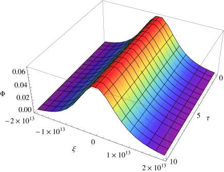
Figure 5: The variation of the $|\Phi|$ with $\xi$ for self-gravitating bright solitons; along with $\alpha=3.67\times 10^{3}$, $\gamma=2.16$, $\mu=1.5$, $k=0.0003$, $\psi_{0}=$0.005, $U=0.001$, $\Omega_{0}=0.04$, $\tau=0$.

Figure 6: The variation of the $|\Phi|$ with $\xi$ and $\tau$ for self-gravitating bright solitons; along with $\alpha=3.67\times 10^{3}$, $\gamma=2.16$, $\mu=1.5$, $k=0.0003$, $\psi_{0}=$0.005, $U=0.001$, $\Omega_{0}=0.04$, $\tau=0$.

where $U$ is the propagation speed, $\psi_{0}$ is the envelope amplitude, $\Omega_{0}$ oscillating frequency for $U=0$ and $W$ is the soliton width which can be defined as $W=\sqrt{2|P/Q|/\psi_{0}}$. The self-gravitating bright envelope soliton depicted in Figs 6 and 6, clearly indicates that the shape of the self-gravitating bright envelope solitons is not affected by any external perturbation through the time evolution. So, the self-gravitating bright envelope solitons are modulationally stable.

V Discussion

In this work, we have investigated the amplitude modulation of IAWs in an unmagnetized three components SG-DQPS comprising of inertialess degenerate electron species, inertial degenerate light and heavy ion species. A NLS equation is derived by employing the reductive perturbation method that governs the stability, circumstance for the appearance of MI growth rate, and formation of the IAWs envelope solitons in SG-DQPS. The noticeable results found from this theoretical investigation can be outlined as follows:

1. The $\omega$ increases (decreases) with $n_{e0}$ ($n_{l0}$), and also decreases exponentially with the increase of $k$.

2. The IAWs will be stable (unstable) for smaller values of $k$ and $P/Q<0$ (larger values of $k$ and $P/Q>0$).

3. The growth rate decreases with the increase of $n_{e0}$ but it decreases with increase (decrease) of $m_{h}$ ($m_{l}$) for fixed value of $Z_{l}$ and $Z_{h}$, similarly, growth rate decreases with the increase (decrease) of $Z_{l}$ ($Z_{h}$) for fixed value of $m_{h}$ and $m_{l}$ (via $\gamma=Z_{l}m_{h}/Z_{h}m_{l}$).

4. The shape of the self-gravitating bright envelope solitons is not affected by any external perturbation through the time evolution. So, the self-gravitating bright envelope solitons are modulationally stable.

In conclusion, we hope that the results from our present theoretical investigation may be helpful in understanding the nonlinear phenomena in astrophysical compact objects (viz. white dwarf and neutron stars Chandrasekhar1931 ; Fowler1994 ; Shapiro1983 ; Koester1990 ; Koester2002 ; Shukla2011 ).

References

- (1) S. Chandrasekhar, Astrophys. J. 74, 81 (1931).
- (2) R. H. Fowler, J. Astrophys. Astr. 15, 115 (1994).
- (3) S. L. Shapiro and S. A. Teukolsky, Black Holes, White Dwarfs and Neutron Stars: The Physics of Compact Objects (John Wiley & Sons, New York, 1983).
- (4) D. Koester and G. Chanmugam, Rep. Prog. Phys. 53, 837 (1990).
- (5) D. M. S. Zaman, M. Amina, P. R. Dip, and A. A. Mamun, Eur. Phys. J. Plus 132, 457 (2017).
- (6) D. Koester, Astron. Astrophys. Rev. 11, 33 (2002).
- (7) P. K. Shukla and B. Eliasson, Rev. Mod. Phys. 83, 885 (2011).
- (8) R. P. Drake, Phys. Plasmas 16, 055501 (2009).
- (9) R. P. Drake, Phys. Plasmas 63, 28 (2010).
- (10) S. H. Glenzer and R. Redmer, Rev. Mod. Phys. 81, 1625 (2009).
- (11) R. S. Fletcher, X. L. Zhang, and S. L. Rolston, Phys. Rev. Lett. 96, 105003 (2006).
- (12) T. C. Killian, Nature (London). 441, 297 (2006).
- (13) A. Vanderburg, J. A. Johnson, S. Rappaport, A. Bieryla, J. Irwin, J. A. Lewis, D. Kipping, W. R. Brown, P. Dufour, D. R. Ciardi, R. Angus, L. Schaefer, D. W. Latham, D. Charbonneau, C. Beichman, J. Eastman, N. McCrady, R. A. Wittenmyer, and J. T. Wright, Nature 526, 546 (2015).
- (14) A. Witze, Nature 510, 196 (2014).
- (15) N. A. Chowdhury, A. Mannan, M. M. Hasan, and A. A. Mamun, Chaos 27, 093105 (2017).
- (16) S. Sultana and I. Kourakis, Plasma Phys. Control. Fusion 53, 045003 (2011).
- (17) M. Asaduzzaman, A. Mannan, A.A. Mamun, Phys. Plasmas 24, 052102 (2017).
- (18) A. A. Mamun, Phys. Plasmas 24, 102306 (2017).
- (19) N. A. Chowdhury, M. M. Hasan, A. Mannan, and A. A. Manun, Vacuum 147, 31 (2018).
- (20) S. Islam, S. Sultana, and A. A. Mamun, Phys. Plasmas 24, 092115 (2017).
- (21) T. Taniuti and N. Yajima, J. Math. Phys. 10, 1369 (1969).
- (22) N. A. Chowdhury, A. Mannan, and A. A. Mamun, Phys. Plasmas 24, 113701 (2017).
- (23) R. Fedele and H. Schamel, Eur. Phys. J. B 27, 313 (2002).
- (24) I. Kourakis and P.K. Shukla, Nonlinear Proc. Geophys. 12, 407 (2005).
- (25) R. Fedele and H. Schamel, Eur. Phys. J. B 27, 313 (2002).