Terminal Iterative Learning Control for Autonomous Aerial Refueling under Aerodynamic Disturbances

Nomenclature

${\Delta\mathbf{F}_{0}}$	=	Bow wave disturbance force
$\Delta{\mathbf{p}}_{\text{dr}}^{\text{e}}$	=	Drogue position offsets from equilibrium position
$\Delta{\mathbf{p}}_{\text{dr/pr}}$	=	Position error between drogue and probe
$\Delta{\mathbf{p}}_{\text{dr/pr}}\left(T\right)$	=	Terminal position error
$\Delta R_{\text{dr/pr}}$	=	Radial error between hose and drogue
$F_{\text{T}}$	=	Tanker joint frame
$\mathbf{F}$${}_{\text{r}}$, $\mathbf{F}$${}_{\text{hd}}$	=	Disturbance forces on receiver and hose-drogue
$\mathbf{F}$${}_{\text{bow}}$	=	Disturbance force from bow wave effect
${\mathbf{p}}_{\text{dr}}\left(t\right)$, ${\mathbf{p}}_{\text{pr}}\left(t\right)$	=	Current positions of drogue and probe
${\mathbf{p}}_{\text{dr}}\left(T\right)$, ${\mathbf{p}}_{\text{pr}}\left(T\right)$	=	Terminal positions of drogue and probe
${\mathbf{p}}_{\text{dr}}^{\text{e0}}$	=	Drogue initial equilibrium position
$\mathbb{R}$, $\mathbb{R}_{+}$	=	Real number set and positive real number set
$R_{\text{C}}$	=	Threshold radius for a successful docking attempt
$T$	=	Terminal time of a docking attempt
$\mathbf{\hat{u}}_{\text{pr}}$	=	Reference trajectory for autopilot

I Introduction

Aerial refueling has demonstrated significant benefits to aviation by extending the range and endurance of aircraft Nalepka-2005-1 . The development of autonomous aerial refueling (AAR) techniques for unmanned aerial vehicles (UAVs) makes new missions and capabilities possible Dibley-2007-2 , like the ability for long range or long time flight. As the most widely used aerial refueling method, the probe-drogue refueling (PDR) system is considered to be more flexible and compact than other refueling systems. However, a drawback of PDR is that the drogue is passive and susceptible to aerodynamic disturbances AAR-2014 . Therefore, it is difficult to design an AAR system to control the probe on the receiver to capture the moving drogue within centimeter level in the docking stage.

It used to be thought that the aerodynamic disturbances in the aerial refueling mainly include the tanker vortex, wind gust, and atmospheric turbulence. According to NASA Autonomous Aerial Refueling Demonstration (AARD) project Dibley-2007-2 , the forebody flow field of the receiver may also significantly affect the docking control of AAR, which is called “the bow wave effect” Bhandari-2013-8 . As a result, the modeling and simulation methods for the bow wave effect were studied in our previous works dai2016modeling ; wei2016drogue . Since the obtained mathematical models are somewhat complex and there may be some uncertain factors in practice, this paper aims to use a model-free method to compensate for the docking error caused by aerodynamic disturbances including the bow wave effect.

Most of the existing studies on AAR docking control do not consider the bow wave effect. In tandale2006trajectory ; zhu2016vision ; liu2017modeling , the drogue is assumed to be relatively static (or oscillates around the equilibrium) and not affected by the flow field of the receiver forebody. However, in practice, the receiver aircraft is affected by aerodynamic disturbances, and the drogue is affected by both the wind disturbances and the receiver forebody bow wave. As a major difficulty in the control of AAR, the aerodynamic disturbances, especially the bow wave effect, attract increasing attention in these years. In Vortex-1 ; lee2013estimation , the wind effects from the tanker vortex, the wind gust, and the atmospheric turbulence are analyzed, and in dai2016modeling ; wei2016drogue ; Khan-2014-9 , the modeling and simulation methods for the receiver forebody bow wave effect are studied, but no control methods are proposed. In Bhandari-2013-8 , simulations show that the bow wave effect can be compensated by adding an offset value to the reference trajectory, but the method for obtaining the offset value is not given.

Since the accurate mathematical models for the aerodynamic disturbances are usually difficult to obtain dai2016modeling , iterative learning control (ILC) is a possible choice for the docking control of AAR. According to bristow2006survey , the ILC is a model-free control method which can improve the performance of a system by learning from the previous repetitive executions or iterations. ILC methods have been proved to be effective to solve the control problems for complex systems with no need for the exact mathematical model ahn2007iterative . For an actual AAR system, the relative position between the probe and the drogue is usually measured by vision localization methods valasek2005vision whose measurement precision depends on the relative distance (higher precision in a closer distance). Therefore, compared with the trajectory data, the terminal positions of the probe and the drogue are usually easier to measure in practice. As a result, terminal iterative learning control (TILC) methods are suitable for AAR systems because TILC methods need only the terminal states or outputs instead of the whole trajectories chen1999iterative ; chi2014improved .

This paper studies the model of the probe-drogue aerial refueling system under aerodynamic disturbances, and proposes a docking control method based on TILC to compensate for the docking errors caused by aerodynamic disturbances. In the ATP-56(B) issued by NATO NATO-2004-3 , chasing the drogue directly is identified as a dangerous operation which may cause the overcontrol of the receiver. Therefore, the proposed TILC controller is designed by imitating the docking operations of human pilots to predict the terminal position of the drogue with an offset to compensate for the docking errors caused by aerodynamic disturbances. The designed controller works as an additional unit for the trajectory generation of the original autopilot system. Simulations based on our previously published MATLAB/SIMULINK environment dai2016modeling ; wei2016drogue show that the proposed control method has a fast learning speed to achieve a successful docking control under aerodynamic disturbances including the bow wave effect.

The paper is organized as follows. Section II gives comprehensive problem description and model analysis of a PDR system. Section III describes the details of the TILC controller design and the convergence analysis. Section IV gives simulations with the proposed TILC method. In the end, Section V presents the conclusions.

II Problem Formulation

II.1 Frames and Notations

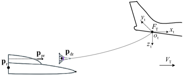
Figure 1: Simplified schematic diagram of PDR systems.

Since the tanker moves at a uniform speed in a straight and level line during the docking stage of AAR, a frame fixed to the tanker body can be treated as an inertial reference frame to describe the relative motion between the receiver and the drogue. As shown in Fig. 1, a tanker joint frame $F_{\text{T}}$ is defined with the origin $O_{\text{t}}$ fixed to the joint between the tanker body and the hose. $F_{\text{T}}$ is a right-handed coordinate system, whose $x_{\text{t}}$ horizontally points to the flight direction of the tanker, $z_{\text{t}}$ vertically points to the ground, and $y_{\text{t}}$ points to the right. For simplicity, the following rules are defined:

(i) All position or state vectors are defined under the tanker joint frame $F_{\text{T}}$, unless explicitly stated.

(ii) The drogue position vector is expressed as ${\mathbf{p}}_{\text{dr}}\triangleq\left[x_{\text{dr}}\;y_{\text{dr}}\;z_{\text{dr}}\right]^{\text{T}}$, and the probe position vector is ${\mathbf{p}}_{\text{pr}}\triangleq\left[x_{\text{pr}}\;y_{\text{pr}}\;z_{\text{pr}}\right]^{\text{T}}$. In a similar way, the position error between the probe and the drogue is expressed as

$$\Delta{\mathbf{p}}_{\text{dr/pr}}\left(t\right)\triangleq{\mathbf{p}}_{\text{dr}}\left(t\right)-{\mathbf{p}}_{\text{pr}}\left(t\right)$$ (1)

whose decomposition form is represented by $\Delta{\mathbf{p}}_{\text{dr/pr}}\triangleq[\Delta x_{\text{dr/pr}}\;\Delta y_{\text{dr/pr}}\;\Delta z_{\text{dr/pr}}]^{\text{T}}$ .

(iii) One docking attempt ends at the terminal time $T\in\mathbb{R}_{+}$ when the probe contacts with the central plane of the drogue ($\Delta x_{\text{dr/pr}}=0$) for the first time, which is defined as

$$T=\min_{t}\left\{\Delta x_{\text{dr/pr}}\left(t\right)=0\right\}.$$ (2)

The value at time $t=T$ is called the terminal value. For example, ${\mathbf{p}}_{\text{dr}}\left(T\right)$ is the terminal position of the drogue and $\Delta{\mathbf{p}}_{\text{dr/pr}}\left(T\right)$ is the terminal position error.

(iv) The value in the $k^{\text{th}}$ docking attempt is marked by a right superscript. For example, ${\mathbf{p}}_{\text{dr}}^{\left(k\right)}$ denotes the drogue position ${\mathbf{p}}_{\text{dr}}$ in the $k^{\text{th}}$ docking attempt, $T^{\left(k\right)}$ denotes the $k^{\text{th}}$ terminal time, and ${\mathbf{p}}_{\text{dr}}^{\left(k\right)}\left(T^{\left(k\right)}\right)$ denotes the $k^{\text{th}}$ terminal position of the drogue.

II.2 System Overview

The overall structure of the AAR system proposed in this paper is shown in Fig. 2, where the whole AAR system is divided into two parts: the mathematical model and the control system. The AAR Mathematical model contains three components: the aerodynamic disturbance model, the hose-drogue dynamic model, and the receiver dynamic model; the control system contains two components: the autopilot and the TILC controller. The autopilot focuses on stabilizing the aircraft attitude and tracking the given reference trajectory, and the TILC controller works as a human pilot that learns from historical experience and sends trajectory commands to the autopilot. This paper focuses on the design of the TILC controller.

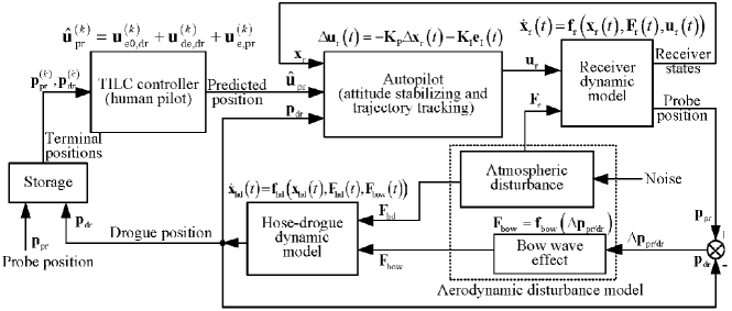
Figure 2: Overall structure of the AAR system.

II.3 Mathematical Model

II.3.1 Aerodynamic Disturbance Model

The aerodynamic disturbances will change the flow field around the receiver and the drogue, then produce disturbance forces on them to affect their relative motions. There are mainly two sources of aerodynamic disturbances: one is from the atmospheric environment such as the tanker vortex, the wind gust and the atmospheric turbulence Vortex-1 ; the other is from the bow wave flow field of the receiver forebody. In an AAR system, the receiver mainly suffers the atmospheric disturbance force $\mathbf{F}$${}_{\text{r}}\in\mathbb{R}^{3}$, while the hose-drogue suffers both the atmospheric disturbance force $\mathbf{F}$${{}_{\text{hd}}}\in\mathbb{R}^{3}$ and the bow wave disturbance force $\mathbf{F}$${}_{\text{bow}}\in\mathbb{R}^{3}$.

The modeling and simulation methods for $\mathbf{F}$${}_{\text{r}}$ and $\mathbf{F}$${{}_{\text{hd}}}$ have been well studied in the existing literature, where the detailed mathematical expression for $\mathbf{F}$${}_{\text{r}}$ can be found in Vortex-1 , the detailed mathematical expression for $\mathbf{F}$${{}_{\text{hd}}}$ can be found in dai2016modeling Vortex-1 . The bow wave disturbance force $\mathbf{F}$${}_{\text{bow}}$, according to dai2016modeling , is determined by the position error between the drogue and the probe $\Delta{\mathbf{p}}_{\text{dr/pr}}$, which can be expressed as

$${\mathbf{F}}_{\text{bow}}{=\mathbf{f}}_{\text{bow}}\left(\Delta{\mathbf{p}}_{\text{dr/pr}}\right)$$ (3)

where ${\mathbf{f}}_{\text{bow}}\left(\cdot\right)$ is the bow wave effect function whose expression can be obtained by the method proposed in dai2016modeling .

Among these disturbances, $\mathbf{F}$${}_{\text{r}}$ and $\mathbf{F}$${{}_{\text{hd}}}$ are independent of the states of the AAR system, and the corresponding control methods are mature; $\mathbf{F}$${}_{\text{bow}}$ is strongly coupled with the system output $\Delta{\mathbf{p}}_{\text{dr/pr}}$, the control strategy for which is challenging and still lacking. Therefore, this paper puts more effort on the control of the bow wave effect.

II.3.2 Hose-drogue Model

The soft hose can be modeled by a finite number of cylinder-shaped rigid links based on the finite-element theory hose-link-model . Then, the hose-drogue dynamic equation can be written as

$$\left\{\begin{array}[]{l}{\mathbf{{\dot{x}}}}_{\text{hd}}\left(t\right)={\mathbf{f}{{}_{\text{hd}}}}\left({{\mathbf{x}_{\text{hd}}}\left(t\right),}\mathbf{F}_{\text{hd}}\left(t\right),\mathbf{F}_{\text{bow}}\left(t\right)\right)\\ {\mathbf{p}_{\text{dr}}}\left(t\right)={\mathbf{g}{{}_{\text{hd}}}}\left({\mathbf{x}_{\text{hd}}}\left(t\right)\right)\end{array}\right.$$ (4)

where ${\mathbf{f}{{}_{\text{hd}}}}\left(\cdot\right)$ is a nonlinear vector function, $\mathbf{x}_{\text{hd}}$ is the hose-drogue state vector, and $\mathbf{F}_{\text{hd}}\left(t\right)$ and $\mathbf{F}_{\text{bow}}\left(t\right)$ are the disturbance forces acting on the drogue. The dimensions of $\mathbf{x}_{\text{hd}}$ and ${\mathbf{f}{{}_{\text{hd}}}}\left(\cdot\right)$ depend on the number of the links that the hose is divided into.

The most concerned value in the TILC method is the terminal position of the drogue. Therefore, it is necessary to study the terminal state of the hose-drogue system (4). According to wei2016drogue , when there is no random disturbance, the drogue will eventually settle at an equilibrium position marked as ${\mathbf{p}}_{\text{dr}}^{\text{e0}}$. Then, under the bow wave effect, the drogue will be pushed to a new terminal position ${\mathbf{p}}_{\text{dr}}\left(T\right)$. The drogue position offset $\Delta{\mathbf{p}}_{\text{dr}}^{\text{e}}\in\mathbb{R}^{3}$ is defined as

$$\Delta{\mathbf{p}}_{\text{dr}}^{\text{e}}={\mathbf{p}}_{\text{dr}}\left(T\right)-{\mathbf{p}}_{\text{dr}}^{\text{e0}}$$ (5)

where $\Delta{\mathbf{p}}_{\text{dr}}^{\text{e}}$ is further determined by the strength of terminal bow wave disturbance force $\mathbf{F}$${}_{\text{bow}}\left(T\right)$ as

$$\Delta{\mathbf{p}}_{\text{dr}}^{\text{e}}={\mathbf{f}_{\text{dr}}}\left({\mathbf{F}}_{\text{bow}}\left(T\right)\right).$$ (6)

Then, substituting Eq. (3) into Eq. (6) yields

$$\Delta{\mathbf{p}}_{\text{dr}}^{\text{e}}={\mathbf{f}_{\text{dr}}}\left({\mathbf{f}}_{\text{bow}}\left(\Delta{\mathbf{p}}_{\text{dr/pr}}\left(T\right)\right)\right)\triangleq{\mathbf{\bar{f}}}_{\text{dr}}\left(\Delta{\mathbf{p}}_{\text{dr/pr}}\left(T\right)\right).$$ (7)

Noticing that $\Delta{\mathbf{p}}_{\text{dr/pr}}\left(T\right)\approx\mathbf{0}$, the Taylor Expansion can be applied to Eq. (7), which results in

$$\Delta{\mathbf{p}}_{\text{dr}}^{e}\approx\mathbf{m}_{0}+\mathbf{M}_{1}\cdot\Delta{\mathbf{p}}_{\text{dr/pr}}\left(T\right)$$ (8)

where

$$\mathbf{m}_{0}\triangleq{\mathbf{\bar{f}}}_{\text{dr}}\left(\mathbf{0}\right),\;\mathbf{M}_{1}\triangleq\left.\frac{\partial{\mathbf{\bar{f}}}_{\text{dr}}\left(\mathbf{x}\right)}{\partial\mathbf{x}}\right|_{\mathbf{x=0}}.$$ (9)

In practice, the drogue is sensitive to the aerodynamic disturbances, and the actual terminal position of the drogue always oscillates around its stable position. Therefore, a bounded disturbance term $\mathbf{v}_{\text{dr}}\in\mathbb{R}^{3}$ should be added to Eq. (7) as

$$\Delta{\mathbf{p}}_{\text{dr}}^{\text{e}}=\mathbf{m}_{0}+\mathbf{M}_{1}\cdot\Delta{\mathbf{p}}_{\text{dr/pr}}\left(T\right)+\mathbf{v}_{\text{dr}}$$ (10)

where $\left\|\mathbf{v}_{\text{dr}}\right\|\leq B_{\text{dr}}$ represents the position fluctuation of the drogue due to random disturbances such as atmospheric turbulence. According to Eq. (10), there is a functional relationship between the terminal docking error $\Delta{\mathbf{p}}_{\text{dr/pr}}\left(T\right)$ and the drogue bow wave offset $\Delta{\mathbf{p}}_{\text{dr}}^{\text{e}}$. Therefore, it is possible to use TILC methods to compensate for the bow wave position offset $\Delta{\mathbf{p}}_{\text{dr}}^{\text{e}}$ with the terminal docking error $\Delta{\mathbf{p}}_{\text{dr/pr}}\left(T\right)$.

The detailed mathematical expression of ${\mathbf{\bar{f}}}_{\text{dr}}\left(\cdot\right)$ can be obtained through methods in dai2016modeling , then the Jacobian matrix $\mathbf{M}_{1}$ can be obtained from Eq. (9). Since ${\mathbf{\bar{f}}}_{\text{dr}}\left(\cdot\right)$ is monotonically decreasing along each axial direction, for the receiver aircraft with symmetrical forebody layout, it is easy to verify that $\mathbf{M}_{1}$ is a negative definite matrix.

II.3.3 Receiver Aircraft Model

As previously mentioned, in the docking stage, the tanker joint frame $F_{\text{T}}$ can be simplified as an inertial frame. Under this situation, the commonly used aircraft modeling methods as presented in AirContrl can be applied to the receiver aircraft with the following form

$$\left\{\begin{array}[]{l}{\mathbf{{\dot{x}}}}_{\text{r}}\left(t\right)={\mathbf{f}}_{\text{r}}\left({\mathbf{x}}_{\text{r}}{\left(t\right),\mathbf{F}}_{\text{r}}{\left(t\right),}\boldsymbol{u}_{\text{r}}\left(t\right)\right)\\ \mathbf{p}{{}_{\text{pr}}}\left(t\right)={\mathbf{g}_{\text{pr}}}\left({\mathbf{x}}_{\text{r}}\left(t\right)\right)\end{array}\right.$$ (11)

where ${\mathbf{f}}_{\text{r}}\left(\cdot\right)$ is a nonlinear function, ${\mathbf{x}}_{\text{r}}$ is the state of the receiver and $\mathbf{u}_{\text{r}}$ is the control input of the receiver aircraft.

Since the nonlinear model (11) is too complex for controller design, a linearization method AirContrl is applied to Eq. (11) to simplify the receiver dynamic model. Assume the receiver equilibrium state is $\mathbf{x}_{\text{r0}}$ and the trimming control is $\boldsymbol{u}_{\text{r0}}$, then the linear model can be expressed as

$$\left\{\begin{array}[]{l}\Delta{\mathbf{{\dot{x}}}}_{\text{r}}\left(t\right)=\mathbf{A}_{\text{r}}\cdot\Delta{\mathbf{x}_{\text{r}}\left(t\right)}+\mathbf{B}_{\text{r}}\cdot\Delta\boldsymbol{u}_{\text{r}}\left(t\right)+\mathbf{G}_{\text{r}}\cdot{\mathbf{F}_{\text{r}}\left(t\right)}\\ \Delta\mathbf{p}{{}_{\text{pr}}}\left(t\right)=\mathbf{C}_{\text{r}}\cdot\Delta{\mathbf{x}_{\text{r}}}\left(t\right)\end{array}\right.$$ (12)

where $\Delta{\mathbf{x}_{\text{r}}\triangleq\mathbf{x}_{\text{r}}-}\mathbf{x}_{\text{r0}}$ is the state vector of the linearized system, $\Delta\boldsymbol{u}_{\text{r}}\triangleq\boldsymbol{u}_{\text{r}}-\boldsymbol{u}_{\text{r0}}$ is the linearized control input vector and $\Delta\mathbf{p}$${}_{\text{pr}}$$\triangleq\mathbf{p}$${}_{\text{pr}}$$-\mathbf{p}{{}_{\text{pr0}}}$ is the probe position offset from the initial probe position $\mathbf{p}{{}_{\text{pr0}}}$.

II.4 Control System

II.4.1 Autopilot

Based on the linear model (12), the autopilot can be simplified as a state feedback controller lee2013estimation in the form as

$$\Delta\boldsymbol{u}_{\text{r}}\left(t\right) = -\mathbf{K}_{\text{P}}\cdot\Delta{\mathbf{x}_{\text{r}}\left(t\right)}-\mathbf{K}_{\text{I}}\cdot\mathbf{e}_{\text{I}}\left(t\right)$$ (13)

$$\mathbf{\dot{e}}_{\text{I}}\left(t\right) = \mathbf{p}{{}_{\text{pr}}\left(t\right)}-\mathbf{\hat{u}}_{\text{pr}}\left(t\right)$$ (14)

where $\mathbf{\hat{u}}_{\text{pr}}\left(t\right)\in\mathbb{R}^{3}$ is the reference trajectory vector of the probe, $\mathbf{K}_{\text{P}}$ and $\mathbf{K}_{\text{I}}$ are the gain matrices. Essentially, Eq. (13) is a PI controller, where $-\mathbf{K}_{\text{P}}\cdot\Delta{\mathbf{x}_{\text{r}}}\left(t\right)$ is the state feedback control term for stabilizing the aircraft, and ${-}\mathbf{K}_{\text{I}}\cdot\mathbf{e}_{\text{I}}\left(t\right)$ is the integral control term for tracking the given trajectory. Since it is very convenient to obtain $\mathbf{K}_{\text{P}}$ and $\mathbf{K}_{\text{I}}$ through LQR function in MATLAB, the procedures are omitted here. In practice, a saturation function is required for $\mathbf{e}_{\text{I}}\left(t\right)$ in Eq. (13) to slow down the response speed and resist integral saturation. For instance, the approaching speed should be constrained within a reasonable range about 0.5m/s$\sim$1m/s, because the probe should have enough closure speed to open the valve on the drogue safely Dibley-2007-2 .

As analyzed in lee2013estimation ; AirContrl , when the autopilot (13) is well designed and the disturbance force $\mathbf{F}$${{}_{\text{r}}\left(t\right)}\equiv\mathbf{0}$, the tracking error can converge to zero

$$\mathbf{\hat{u}}_{\text{pr}}\left(t\right)-\mathbf{p}{{}_{\text{pr}}}\left(t\right)\rightarrow\mathbf{0},\text{ as }t\rightarrow\infty.$$ (15)

However, in practice, the disturbance force $\mathbf{F}$${{}_{\text{r}}\left(t\right)}\neq\mathbf{0}$ and the terminal time $T\ll\infty$, then the tracking error cannot reach zero at terminal time $T$. Therefore, an error term should be added to Eq. (15) at $T$ as

$$\mathbf{\hat{u}}_{\text{pr}}\left(T\right)-\mathbf{p}{{}_{\text{pr}}}\left(T\right)=\mathbf{v}_{\text{pr}}$$ (16)

where $\mathbf{v}_{\text{pr}}\in\mathbb{R}^{3}$ is a bounded random disturbance term with $\left\|\mathbf{v}_{\text{pr}}\right\|\leq B_{\text{pr}}$. The random disturbance $\mathbf{v}_{\text{pr}}$ may come from the unrepeatable disturbances such as atmospheric turbulence.

II.4.2 Objective of Docking Control

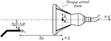
Figure 3: Success and failure criteria of a docking attempt Dibley-2007-2 .

According to Dibley-2007-2 , in each docking attempt, the receiver should follow the drogue for seconds until the hose-drogue levels off. Then, the receiver starts to drive the probe to approach the drogue with a slow constant speed, until the probe hits the central plane of the drogue as shown in Fig. 3. The basic requirement for the AAR system is that the relative position between the probe and the drogue (represented by the docking error $\Delta{\mathbf{p}}_{\text{dr/pr}}$) can reach zero at the terminal time $T$. In practice, the radial error $\Delta R_{\text{dr/pr}}\in\mathbb{R}_{+}$ is an important evaluation index for the docking performance which defined in oyz plane as

$$\Delta R_{\text{dr/pr}}\left(t\right)\triangleq\sqrt{\Delta y_{\text{dr/pr}}^{2}\left(t\right)+\Delta z_{\text{dr/pr}}^{2}\left(t\right)}.$$ (17)

Since the docking error is inevitable due to disturbances, a threshold radius (criterion radius) $R_{\text{C}}\in\mathbb{R}_{+}$ should be defined as

$$\Delta R_{\text{dr/pr}}\left(T\right)<R_{\text{C}}.$$ (18)

If criterion (18) is satisfied, a success docking is declared for this docking attempt Dibley-2007-2 . Otherwise, a failure or miss is declared. In fact, according to the previous definition, there is $\Delta x_{\text{dr/pr}}\left(T\right)\equiv 0$. Therefore, the terminal radial error $\Delta R_{\text{dr/pr}}\left(T\right)$ always equals to the terminal docking error $\Delta{\mathbf{p}}_{\text{dr/pr}}\left(T\right)$.

III TILC Design

As shown in Fig. 2, the role of the TILC controller in AAR system is the same as the human pilot in manned aerial refueling system. The inputs of the TILC controller are the historical terminal positions of the probe ${\mathbf{p}}_{\text{pr}}\left(T\right)$ and the drogue ${\mathbf{p}}_{\text{dr}}\left(T\right)$, and the output is the reference tracking trajectory $\mathbf{\hat{u}}_{\text{pr}}\left(t\right)$ which is further sent to the autopilot.

III.1 TILC Controller

The docking errors of the AAR system are mainly caused by two factors: the drogue offset caused by the bow wave effect as described in Eq. (5); and the tracking error caused by the response lag of the receiver as described in Eq. (16). In order to compensate for these docking errors, a simple and safe control strategy is letting the probe always aims at a predicted fixed position $\mathbf{\hat{u}}_{\text{pr}}^{\left(k\right)}\left(t\right)\equiv\mathbf{\hat{u}}_{\text{pr}}^{\left(k\right)}$ during the docking stage. The predicted position $\mathbf{\hat{u}}_{\text{pr}}^{\left(k\right)}$ for the autopilot should have the following form

$$\mathbf{\hat{u}}_{\text{pr}}^{\left(k\right)}={\mathbf{p}}_{\text{dr}}^{\text{e0,}\left(k\right)}+\mathbf{u}_{\text{de,dr}}^{\left(k\right)}+\mathbf{u}_{\text{e,pr}}^{\left(k\right)}$$ (19)

where ${\mathbf{p}}_{\text{dr}}^{\text{e0,}\left(k\right)}\in\mathbb{R}^{3}$ is the original stable position of the drogue, $\mathbf{u}_{\text{de,dr}}^{\left(k\right)}\in\mathbb{R}^{3}$ is an estimation term for the drogue position offset, and $\mathbf{u}_{\text{e,pr}}^{\left(k\right)}\in\mathbb{R}^{3}$ is an ILC term to compensate for the tracking error of the probe. Note that, since ${\mathbf{p}}_{\text{dr}}^{\text{e0,}\left(k\right)}$ can be directly measured during the flight, it is treated as a known parameter here. Then, $\mathbf{u}_{\text{de,dr}}^{\left(k\right)}$ and $\mathbf{u}_{\text{e,pr}}^{\left(k\right)}$ should be updated in each iteration, and the updating laws are given below.

(1) the updating law of $\mathbf{u}_{\text{de,dr}}^{\left(k\right)}$ is given by

$$\mathbf{u}_{\text{de,dr}}^{\left(k\right)}=\mathbf{K}_{\alpha}\cdot\mathbf{u}_{\text{de,dr}}^{\left(k-1\right)}+\left(\mathbf{I}-\mathbf{K}_{\alpha}\right)\cdot\Delta{\mathbf{p}}_{\text{dr}}^{\text{e,}\left(k-1\right)}$$ (20)

where $\mathbf{K}_{\alpha}=\text{diag}\left(k_{\alpha_{1}},k_{\alpha_{2}},k_{\alpha_{3}}\right)$ with $k_{\alpha_{1}},k_{\alpha_{2}},k_{\alpha_{3}}\in\left(0,1\right)$ is a constant diagonal matrix, and $\Delta{\mathbf{p}}_{\text{dr}}^{\text{e}}$ is the drogue terminal offset position as defined in Eq. (5) whose iterative feature can be written as

$$\Delta{\mathbf{p}}_{\text{dr}}^{\text{e,}\left(k\right)}\triangleq\mathbf{p}{{}_{\text{dr}}^{(k)}}\left(T^{\left(k\right)}\right)-{\mathbf{p}}_{\text{dr}}^{\text{e0,}\left(k\right)}.$$ (21)

(2) the updating law of $\mathbf{u}_{\text{e,pr}}^{\left(k\right)}$ is given by

$$\mathbf{u}_{\text{e,pr}}^{\left(k\right)}=\mathbf{u}_{\text{e,pr}}^{\left(k-1\right)}+\mathbf{K}_{p}\cdot\mathbf{e}_{\text{pr}}^{(k-1)}$$ (22)

where $\mathbf{K}_{p}=\text{diag}\left(k_{p_{1}},k_{p_{2}},k_{p_{3}}\right)$ is a constant diagonal matrices with $k_{p_{1}},k_{p_{2}},k_{p_{3}}\in\left(0,1\right)$ and $\mathbf{e}_{\text{pr}}$ represents the probe terminal tracking error with the $k^{\text{th}}$ iterative feature defined as

$$\mathbf{e}_{\text{pr}}^{(k)}\triangleq{\mathbf{p}}_{\text{dr}}^{\text{e0,}\left(k\right)}+\mathbf{u}_{\text{de,dr}}^{\left(k\right)}-\mathbf{p}{{}_{\text{pr}}^{(k)}}\left(T^{\left(k\right)}\right).$$ (23)

III.2 Convergence Analysis

The following theorem provides the convergence condition under which one can conclude the convergence property of the designed TILC controller in Eq. (19).

Theorem 1. Consider the AAR system described by Eqs. (4)(11)(13) with the structure shown in Fig. 2. Suppose (i) the autopilot of the receiver aircraft in Eq. (13) is well designed, and the probe terminal position satisfies Eq. (16); (ii) the TILC controller is designed as Eq. (19), and its parameters satisfy

$$0\leq k_{\alpha_{i}}<1,\text{ }0<k_{p_{i}}\leq 1,\text{ }i=1,2,3.$$ (24)

Then, through the repetitive docking attempts, the docking error $\Delta{\mathbf{p}}_{\text{dr/pr}}^{\left(k\right)}\left(T^{\left(k\right)}\right)$ will converge to a bound

$$\lim_{k\rightarrow\infty}\left\|\Delta{\mathbf{p}}_{\text{dr/pr}}^{\left(k\right)}\left(T^{\left(k\right)}\right)\right\|\leq B_{\text{dr/pr}}$$ (25)

where

$$B_{\text{dr/pr}}=2\sqrt{B_{\text{pr}}^{2}+B_{\text{dr}}^{2}}$$ (26)

in which $B_{\text{dr}}$ is the random disturbance bound of the drogue position fluctuation as defined in Eq. (10) and $B_{\text{pr}}$ is the random disturbance bound of the probe tracking error as defined Eq. (16). In particular, if the random disturbances are negligible, i.e., $B_{\text{dr}}=0$, $B_{\text{pr}}=0$, then the docking error will converge to zero as

$$\left\|\Delta{\mathbf{p}}_{\text{dr/pr}}^{\left(k\right)}\left(T^{\left(k\right)}\right)\right\|\rightarrow 0\text{, as }k\rightarrow\infty.$$ (27)

Proof. See Appendix A. $\square$

III.3 Discussion

Essentially, the term $\mathbf{u}_{\text{de,dr}}^{\left(k\right)}$ works as a low-pass filter, which is expected to provide a smooth and robust estimation of the drogue offset caused by disturbances. Then, with this term in $\mathbf{\hat{u}}_{\text{pr}}^{\left(k\right)}$, the drogue offset can be compensated. The low-pass filter is adopted instead of using the drogue offset position directly, which is because the drogue is sensitive to disturbances.

The initial value for the proposed TILC method in Eq. (19) should be set to zero ($\mathbf{u}_{\text{de,dr}}^{\left(0\right)}=\mathbf{0}$, $\mathbf{u}_{\text{e,pr}}^{\left(0\right)}=\mathbf{0}$) when there is no historical learning data. In practice, $\mathbf{u}_{\text{de,dr}}^{\left(0\right)}$ has physical significance, namely the drogue position offset caused by the receiver forebody flow field. Therefore, the initial value for $\mathbf{u}_{\text{de,dr}}^{\left(0\right)}$ can be estimated according to the historical learning data, the experience of human pilots, or the calculation result from the hose-drogue model hose-link-model and the bow wave effect model dai2016modeling . With the pre-estimated initial value, the iteration speed of the proposed TILC method can be improved.

Unlike other conventional ILC methods, the proposed TILC method does not require the exact value of the terminal time $T$ and does not require $T$ to be the same between iterations. It only requires the terminal positions of the drogue and the probe, which is practical for an actual AAR system.

IV Simulation and Verification

IV.1 Simulation Configuration

A MATLAB/SIMULINK-based simulation environment has been developed to simulate the docking stage of the AAR. The detailed introduction of the modeling methods and the simulation parameters can be found in the authors’ previous work dai2016modeling . A video has also been released to introduce the AAR simulation environment and demonstrate the TILC simulation results. The URL of the video is https://youtu.be/VoplDA6D5fA.

IV.2 TILC Simulation Results

IV.2.1 Iterative Learning Process

In order to verify the effectiveness of the proposed TILC method, all the initial values in Eq. (19) are set zeroes as $\mathbf{u}_{\text{de,dr}}^{\left(0\right)}=\mathbf{0}$, $\mathbf{u}_{\text{e,pr}}^{\left(0\right)}=\mathbf{0}$, and the learning procedures are shown in Fig. 4.

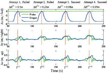
Figure 4: Learning process with the proposed TILC method.

In Fig. 4, there are four docking attempts performed in sequence (the four docking attempts start at time 50s, 100s, 150s and 200s respectively), where the first two docking attempts fail, and the following two attempts both succeed. In each attempt, the probe moves close to until contact with the drogue at $T^{\left(k\right)}$ (marked by the vertical dotted lines), then the probe returns to the standby postilion and gets ready for the next docking attempt.

In the first docking attempt as shown in Fig. 4, the receiver remains at the standby position (5m behind the drogue, with simulation time from 50s to 60s) to observe the drogue movement and estimate the equilibrium position of the drogue. Then, the receiver approaches the drogue to perform a docking attempt during the simulation time from 60s to 71s in Fig. 4. The docking control ends at the terminal time $T^{\left(1\right)}=71s$, and this docking attempt is declared as a failure because the radial error $\Delta R_{\text{dr/pr}}^{\left(1\right)}=0.5m$ is larger than the desired radial error threshold $R_{C}=0.15\text{m}$.

With more docking attempts (not presented in Fig. 4) are simulated, a docking success rate over 90% will be obtained under the given threshold $R_{C}=0.15\text{m}$. According to the Monte Carlo simulations, the success rate depends on many factors including the docking error threshold $R_{C}$, the strength of the atmospheric turbulence, and other random disturbances. The simulation results are consistent with results in Dibley-2007-2 Bhandari-2013-8 . When the aerodynamic disturbances are strong, both the drogue position oscillation and the receiver tracking error will be significant, then the success rate will be low.

IV.2.2 Aerodynamic Disturbance Simulations

Fig. 5 presents the total aerodynamic disturbance force $\mathbf{F}_{\text{total}}=\left[\Delta F_{\text{x}},\Delta F_{\text{y}},\Delta F_{\text{z}}\right]^{\text{T}}$ applied on the drogue during the first docking attempt (50s$\sim$71s) in Fig. 4. In this simulation, the tanker vortex disturbance comes from the model presented in Vortex-1 , the wind gust and the atmospheric turbulence come from the MATLAB/SIMULINK Aerospace Blockset based on the mathematical representations from Military Specification MIL-F-8785C, and the bow wave effect disturbance comes from the authors’ previous work wei2016drogue . When the receiver remains at the standby position (50s$\sim$60s in Fig. 5), the drogue is far away from the receiver and the disturbance forces mainly come from the tanker vortex and the atmospheric turbulence as illustrated on the left half of Fig. 5. As the receiver moves closer to the drogue, the receiver bow wave starts to cause a large disturbance force on the drogue as illustrated on the right half of Fig. 5.

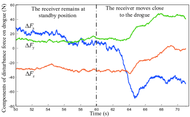
Figure 5: Total aerodynamic disturbing force applied on the drogue.

A comprehensive simulation is performed to verify the performance of the proposed TILC method with the initial value from the previous learning results. In addition to the atmospheric turbulence and the bow wave disturbance as shown in Fig. 5, a wind gust ($5m/s$ in the lateral direction and vertical direction respectively) is added at 100s to verify the control effect of the proposed method under aerodynamic disturbances. The simulation results are presented in Fig. 6.

It can be observed from Fig. 6 that, with a good initial value, the docking control succeeds at the first attempt. Then, the second docking attempt (115s in Fig. 6) fails due to the addition of a strong wind gust at 100s. In the next two docking attempts (165s and 215s in Fig. 6), the controller can rapidly recover and achieve successful docking control without being much affected by the wind gust disturbance. The simulation results demonstrate that the proposed TILC method has a certain ability to resist the aerodynamic disturbances.

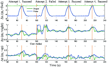
Figure 6: Simulation with the initial value and the wind gust disturbance.

V Conclusions

This paper studies the model of the probe-drogue aerial refueling system under aerodynamic disturbances, and proposes a docking control method based on terminal iterative learning control to compensate for the docking errors caused by aerodynamic disturbances. The designed controller works as an additional unit for the trajectory generation function of the original autopilot system. Simulations based on our previously published simulation environment show that the proposed control method has a fast learning speed to achieve a successful docking control under aerodynamic disturbances including the bow wave effect.

Appendices

V.1 Proof of Theorem 1

First, define the $\mathbf{p}{{}_{\text{pr}}^{\left(k\right)}}\left(T^{\left(k\right)}\right)$ as the probe terminal position in the $k^{\text{th}}$ docking attempt. Then, according to Eq. (16), one has

$$\mathbf{p}{{}_{\text{pr}}^{\left(k\right)}}\left(T^{\left(k\right)}\right)=\mathbf{\hat{u}}_{\text{pr}}^{\left(k\right)}-\mathbf{v}_{\text{pr}}^{\left(k\right)}$$ (28)

where, $\mathbf{\hat{u}}_{\text{pr}}^{\left(k\right)}$ can be further expressed by Eq. (19), which yields

$${\mathbf{p}}_{\text{dr}}^{\text{e0,}\left(k\right)}+\mathbf{u}_{\text{de,dr}}^{\left(k\right)}-\mathbf{p}{{}_{\text{pr}}^{\left(k\right)}}\left(T^{\left(k\right)}\right)=\mathbf{v}_{\text{pr}}^{\left(k\right)}-\mathbf{u}_{\text{e,pr}}^{\left(k\right)}.$$ (29)

Meanwhile, according to the definition of $\mathbf{e}_{\text{pr}}^{(k)}$ in Eq. (23), one has

$$\mathbf{e}_{\text{pr}}^{(k)}=\mathbf{v}_{\text{pr}}^{\left(k\right)}-\mathbf{u}_{\text{e,pr}}^{\left(k\right)}.$$ (30)

Thus, substituting Eq. (22) into Eq. (30) gives

$$\mathbf{e}_{\text{pr}}^{(k)}=\left(\mathbf{I}-\mathbf{K}_{p}\right)\cdot\mathbf{e}_{\text{pr}}^{(k-1)}+\mathbf{\tilde{v}}_{\text{pr}}^{\left(k-1\right)}$$ (31)

where

$$\mathbf{\tilde{v}}_{\text{pr}}^{\left(k-1\right)}\triangleq\mathbf{v}_{\text{pr}}^{\left(k\right)}-\mathbf{v}_{\text{pr}}^{\left(k-1\right)}.$$ (32)

Second, according to Eq. (5), the drogue terminal position $\mathbf{p}{{}_{\text{dr}}^{(k)}}\left(T^{\left(k\right)}\right)$ in the $k^{\text{th}}$ docking attempt is given by

$$\mathbf{p}{{}_{\text{dr}}^{(k)}}\left(T^{\left(k\right)}\right)={\mathbf{p}}_{\text{dr}}^{\text{e0,}\left(k\right)}+\Delta{\mathbf{p}}_{\text{dr}}^{\text{e,}\left(k\right)}$$ (33)

where ${\mathbf{p}}_{\text{dr}}^{\text{e0,}\left(k\right)}$ is the drogue original equilibrium position, and $\Delta{\mathbf{p}}_{\text{dr}}^{\text{e,}\left(k\right)}$ is the terminal position offset. According to Eq. (10), $\Delta{\mathbf{p}}_{\text{dr}}^{\text{e,}\left(k\right)}$ comes from the bow wave effect and can be expressed

$$\Delta{\mathbf{p}}_{\text{dr}}^{\text{e,}\left(k\right)}=\mathbf{m}_{0}+\mathbf{M}_{1}\cdot\Delta{\mathbf{p}}_{\text{dr/pr}}^{\left(k\right)}\left(T^{\left(k\right)}\right)+\mathbf{v}_{\text{dr}}^{\left(k\right)}.$$ (34)

Thus, the docking error along the iteration axis is given by

$$\Delta{\mathbf{p}}_{\text{dr/pr}}^{\left(k\right)}\left(T^{\left(k\right)}\right)=\mathbf{p}{{}_{\text{dr}}^{\left(k\right)}}\left(T^{\left(k\right)}\right)-\mathbf{p}{{}_{\text{pr}}^{\left(k\right)}}\left(T^{\left(k\right)}\right).$$ (35)

Substituting Eqs. (33)(34)(35) into Eqs. (20)(21) gives

$$\Delta{\mathbf{p}}_{\text{dr/pr}}^{\left(k\right)}\left(T^{\left(k\right)}\right)=\mathbf{A}_{1}\cdot\Delta{\mathbf{p}}_{\text{dr/pr}}^{\left(k-1\right)}\left(T^{\left(k-1\right)}\right)+\mathbf{A}_{2}\cdot\mathbf{e}_{\text{pr}}^{(k-1)}+\mathbf{\tilde{v}}_{\text{dr}}^{\left(k-1\right)}$$ (36)

where

$$\mathbf{A}_{1} \triangleq \left(\mathbf{M}_{1}-\mathbf{I}\right)^{-1}\left(\mathbf{M}_{1}-\mathbf{K}_{\alpha}\right)=\mathbf{I-}\left(\mathbf{I-M}_{1}\right)^{-1}\left(\mathbf{I}-\mathbf{K}_{\alpha}\right)$$ (37)

$$\mathbf{A}_{2} \triangleq \left(\mathbf{M}_{1}-\mathbf{I}\right)^{-1}\left(\mathbf{K}_{p}+\mathbf{K}_{\alpha}-\mathbf{I}\right)$$ (38)

$$\mathbf{\tilde{v}}_{\text{dr}}^{\left(k-1\right)} \triangleq \left(\mathbf{M}_{1}-\mathbf{I}\right)^{-1}\left(\mathbf{v}_{\text{dr}}^{\left(k-1\right)}-\mathbf{v}_{\text{dr}}^{\left(k\right)}\right).$$ (39)

For simplicity, an augmented system is defined as

$$\mathbf{X}^{\left(k\right)}=\mathbf{A\cdot X}^{\left(k-1\right)}+\mathbf{v}^{\left(k-1\right)}$$ (40)

where

$$\mathbf{X}^{\left(k\right)} \triangleq \left[\begin{array}[]{c}\Delta{\mathbf{p}}_{\text{dr/pr}}^{\left(k\right)}\left(T^{\left(k\right)}\right)\\ \mathbf{e}_{\text{pr}}^{(k)}\end{array}\right],\mathbf{v}^{\left(k\right)}\triangleq\left[\begin{array}[]{c}\mathbf{\tilde{v}}_{\text{dr}}^{\left(k\right)}\\ \mathbf{\tilde{v}}_{\text{pr}}^{\left(k\right)}\end{array}\right]$$ (45)

$$\mathbf{A} \triangleq \left[\begin{array}[]{cc}\mathbf{A}_{1}&\mathbf{A}_{2}\\ \mathbf{0}_{3\times 3}&\mathbf{A}_{3}\end{array}\right],\;\mathbf{A}_{3}\triangleq\mathbf{I}-\mathbf{K}_{p}.$$ (48)

Furthermore, Eq. (45) can be written into the following form

$$\mathbf{X}^{\left(k\right)}=\mathbf{A}^{k}\cdot\mathbf{X}^{\left(0\right)}+\sum_{i=0}^{k-1}\mathbf{A}^{i}\mathbf{v}^{\left(k-i\right)}.$$ (49)

Since $\mathbf{M}_{1}$ is a negative definite matrix, according to Eqs. (37)(37)(45), it is easy to verify that the spectral radius of $\mathbf{A}$ is smaller than 1 ($\rho\left(\mathbf{A}\right)<1$) when the following constraint is satisfied

$$0\leq k_{\alpha_{i}}<1,\text{ }0<k_{p_{i}}\leq 1\text{, }i=1,2,3.$$ (50)

Moreover, since the disturbances $\mathbf{v}_{\text{pr}}^{\left(k\right)}$ and $\mathbf{v}_{\text{dr}}^{\left(k\right)}$ are both bounded with $\left\|\mathbf{v}_{\text{pr}}^{\left(k\right)}\right\|\leq B_{\text{pr}}$ and $\left\|\mathbf{v}_{\text{dr}}^{\left(k\right)}\right\|\leq B_{\text{dr}}$, it is easy to obtain from Eqs. (32)(37)(45) that $\mathbf{v}^{\left(k\right)}$ is also bounded with

$$\left\|\mathbf{v}^{\left(k\right)}\right\|\leq 2\sqrt{B_{\text{pr}}^{2}+B_{\text{dr}}^{2}}.$$ (51)

Then, substituting Eq. (51) into Eq. (49) gives

$$\begin{array}[]{ll}\left\|\mathbf{X}^{\left(k\right)}\right\|&\leq\left\|\mathbf{A}\right\|^{k}\left\|\mathbf{X}^{\left(0\right)}\right\|+\sum_{i=0}^{k-1}\left\|\mathbf{A}\right\|^{i}\left\|\mathbf{v}^{\left(k-i\right)}\right\|\\ &\leq\left\|\mathbf{A}\right\|^{k}\left\|\mathbf{X}^{\left(0\right)}\right\|+2\sqrt{B_{\text{pr}}^{2}+B_{\text{dr}}^{2}}\sum_{i=0}^{k-1}\left\|\mathbf{A}\right\|^{i}\\ &=\left\|\mathbf{A}\right\|^{k}\left\|\mathbf{X}^{\left(0\right)}\right\|+2\sqrt{B_{\text{pr}}^{2}+B_{\text{dr}}^{2}}\left(1-\left\|\mathbf{A}\right\|^{k}\right).\end{array}$$ (52)

When the constraint in Eq. (50) is satisfied, one has

$$\rho\left(\mathbf{A}\right)<1\Rightarrow\lim_{k\rightarrow\infty}\left\|\mathbf{A}\right\|^{k}=0$$ (53)

which yields from Eq. (52) that

$$\lim_{k\rightarrow\infty}\left\|\mathbf{X}^{\left(k\right)}\right\|\leq 2\sqrt{B_{\text{pr}}^{2}+B_{\text{dr}}^{2}}.$$ (54)

According to the definition of $\mathbf{X}^{\left(k\right)}$ in Eq. (45), one has

$$\left\|\Delta{\mathbf{p}}_{\text{dr/pr}}^{\left(k\right)}\left(T^{\left(k\right)}\right)\right\|\leq\left\|\mathbf{X}^{\left(k\right)}\right\|.$$ (55)

Combining Eq. (54) and (55) gives

$$\lim_{k\rightarrow\infty}\left\|\Delta{\mathbf{p}}_{\text{dr/pr}}^{\left(k\right)}\left(T^{\left(k\right)}\right)\right\|\leq 2\sqrt{B_{\text{pr}}^{2}+B_{\text{dr}}^{2}}=B_{\text{dr/pr}}.$$ (56)

Thus, the docking error $\Delta{\mathbf{p}}_{\text{dr/pr}}^{\left(k\right)}\left(T^{\left(k\right)}\right)$ will converge to a bound $B_{\text{dr/pr}}$ as $k\rightarrow\infty$. In particular, by substituting $B_{\text{dr}}=0\text{, }B_{\text{pr}}=0$ into Eq. (56), one has $\lim_{k\rightarrow\infty}\left\|\Delta{\mathbf{p}}_{\text{dr/pr}}^{\left(k\right)}\left(T^{\left(k\right)}\right)\right\|=0$.

References

References

-
(1)
Nalepka, J. P. and Hinchman, J. L., “Automated aerial refueling:
extending the effectiveness of unmanned air vehicles,” in “AIAA
Modeling and Simulation Technologies Conference and Exhibit,” AIAA Paper
2005-6005, Aug. 2005,
10.2514/6.2005-6005. -
(2)
Dibley, R. P., Allen, M. J., and Nabaa, N., “Autonomous Airborne
Refueling Demonstration Phase I Flight-Test Results,” in “AIAA
Atmospheric Flight Mechanics Conference and Exhibit,” AIAA Paper 2007-6639,
Aug. 2007,
10.2514/6.2007-6639. -
(3)
Thomas, P. R., Bhandari, U., Bullock, S., Richardson, T. S., and Du Bois,
J. L., “Advances in air to air refuelling,” Progress in
Aerospace Sciences, Vol. 71, 2014, pp. 14–35,
10.1016/j.paerosci.2014.07.001. -
(4)
Bhandari, U., Thomas, P. R., Bullock, S., Richardson, T. S., and du Bois,
J. L., “Bow Wave Effect in Probe and Drogue Aerial Refuelling,” in
“AIAA Guidance, Navigation, and Control Conference,” AIAA Paper
2013-4695, Aug. 2013,
10.2514/6.2013-4695. -
(5)
Dai, X., Wei, Z.-B., and Quan, Q., “Modeling and simulation of bow wave
effect in probe and drogue aerial refueling,” Chinese Journal of
Aeronautics, Vol. 29, No. 2, 2016, pp. 448–461,
10.1016/j.cja.2016.02.001. -
(6)
Wei, Z.-B., Dai, X., Quan, Q., and Cai, K.-Y., “Drogue dynamic model
under bow wave in probe-and-drogue refueling,” IEEE Transactions on
Aerospace and Electronic Systems, Vol. 52, No. 4, 2016, pp. 1728–1742,
10.1109/TAES.2016.140912. -
(7)
Tandale, M. D., Bowers, R., and Valasek, J., “Trajectory tracking
controller for vision-based probe and drogue autonomous aerial refueling,”
Journal of Guidance, Control, and Dynamics, Vol. 29, No. 4, 2006, pp.
846–857,
10.2514/1.19694. -
(8)
Zhu, H., Yuan, S., and Shen, Q., “Vision/GPS-based docking control for
the UAV Autonomous Aerial Refueling,” in “Guidance, Navigation and
Control Conference (CGNCC), 2016 IEEE Chinese,” IEEE, 2016, pp. 1211–1215,
10.1109/CGNCC.2016.7828960. -
(9)
Liu, Z., Liu, J., and He, W., “Modeling and vibration control of a
flexible aerial refueling hose with variable lengths and input constraint,”
Automatica, Vol. 77, 2017, pp. 302–310,
10.1016/j.automatica.2016.11.002. -
(10)
Dogan, A., Lewis, T. A., and Blake, W., “Flight data analysis and
simulation of wind effects during aerial refueling,” Journal of
Aircraft, Vol. 45, No. 6, 2008, pp. 2036–2048,
10.2514/1.36797. -
(11)
Lee, J. H., Sevil, H. E., Dogan, A., and Hullender, D., “Estimation of
receiver aircraft states and wind vectors in aerial refueling,” Journal
of Guidance, Control, and Dynamics, Vol. 37, No. 1, 2013, pp. 265–276,
10.2514/1.59783. -
(12)
Khan, O. and Masud, J., “Trajectory analysis of basket engagement
during aerial refueling,” in “AIAA Atmospheric Flight Mechanics
Conference,” AIAA Paper 2014-0190, Jan. 2014,
10.2514/6.2014-0190. -
(13)
Bristow, D. A., Tharayil, M., and Alleyne, A. G., “A survey of
iterative learning control,” IEEE Control Systems, Vol. 26, No. 3,
2006, pp. 96–114,
10.1109/MCS.2006.1636313. -
(14)
Ahn, H.-S., Chen, Y., and Moore, K. L., “Iterative learning control:
Brief survey and categorization,” IEEE Transactions on Systems, Man,
and Cybernetics, Part C (Applications and Reviews), Vol. 37, No. 6, 2007,
pp. 1099–1121,
10.1109/TSMCC.2007.905759. -
(15)
Valasek, J., Gunnam, K., Kimmett, J., Junkins, J. L., Hughes, D., and Tandale,
M. D., “Vision-based sensor and navigation system for autonomous air
refueling,” Journal of Guidance, Control, and Dynamics, Vol. 28,
No. 5, 2005, pp. 979–989,
10.2514/1.11934. -
(16)
Chen, Y. and Wen, C., Iterative learning control: convergence, robustness
and applications, Springer-Verlag, 1999,
10.1007/BFb0110114. -
(17)
Chi, R., Hou, Z., Jin, S., and Wang, D., “Improved data-driven optimal
TILC using time-varying input signals,” Journal of Process Control,
Vol. 24, No. 12, 2014, pp. 78–85,
10.1016/j.jprocont.2014.07.007. - (18) NATO, “ATP-56(B) Air-to-Air Refuelling,” Tech. rep., NATO, 2010.
-
(19)
Ro, K. and Kamman, J. W., “Modeling and simulation of hose-paradrogue
aerial refueling systems,” Journal of Guidance, Control, and Dynamics,
Vol. 33, No. 1, 2010, pp. 53–63,
10.2514/1.45482. -
(20)
Stevens, B. L. and Lewis, F. L., Aircraft Control and Simulation, John
Wiley & Sons, 2004,
10.1108/aeat.2004.12776eae.001.