Eigen-Inference Precoding for Coarsely Quantized Massive MU-MIMO System with Imperfect CSI

Abstract

This work considers the precoding problem in massive multiuser multiple-input multiple-output (MU-MIMO) systems equipped with low-resolution digital-to-analog converters (DACs). In previous literature on this topic, it is commonly assumed that the channel state information (CSI) is perfectly known. However, in practical applications the CSI is inevitably contaminated by noise. In this paper, we propose, for the first time, an eigen-inference (EI) precoding scheme to improve the error performance of the coarsely quantized massive MU-MIMO systems under imperfect CSI, which is mathematically modeled by a sum of two rectangular random matrices (RRMs): $\sqrt{1-\eta}{\bf{H}}+\sqrt{\eta}{\bf{E}}$. Instead of performing analysis based on the RRM, using Girko s Hermitization trick, the proposed method leverages the block random matrix theory by augmenting the RRM into a block symmetric channel matrix (BSCA). Specially, we derive the empirical distribution of the eigenvalues of the BSCA and establish the limiting spectra distribution connection between the true BSCA and its noisy observation. Then, based on these theoretical results, we propose an EI-based moments matching method for CSI-related noise level ($\eta$) estimation and a rotation invariant estimation method for CSI reconstruction. Based on the cleaned CSI, the quantized precoding problem is tackled via the Bussgang theorem and the Lagrangian multiplier method. The prosed methods are lastly verified by numerical simulations and the results demonstrate the effectiveness of the proposed precoder.

I Introduction

Recent years have witnessed an increasing interest in massive MU-MIMO systems, in which the BS can simultaneously serve a large number of users equipments (UEs) by utilizing hundreds (even thousands) of transmit antennas [1, 2, 3]. As the number of antennas goes to infinity, the performance of classical precoders, e.g., maximum ratio transmission (MRT), zero-forcing (ZF) and water-filling (WF) [4], approach to that of optimal nonlinear ones [5]. On the other hand, gigantic increase in energy consumption, a key challenge to the use of massive MIMO, is brought by scaling up the number of the antennas. An effective way to decrease the energy cost is to equip the BS with low-resolution analog-to-digital converters (ADCs) [6] and DACs [7].

I-A Related Works

The performance of quantized massive MU-MIMO systems has been extensively evaluated in terms of different performance metrics, such as (coded or uncoded) bit error rate (BER) [8, 9, 10], coverage probability [11], [12], and sum rate [13, 14, 15]. For the simplest case that the massive MU-MIMO are deployed with 1-bit ADCs or DACs, it has been shown in a recent study [16] that, compared with massive MIMO systems with ideal DACs, the sum rate loss in 1-bit massive MU-MIMO systems can be compensated by disposing approximately 2.5 times more antennas at the BS. Meanwhile, the authors in [17] presented a quantized constant envelope (QCE) precoder, which can significantly reduce the power consumption of large-size communication systems. For frequency-selective MU-MIMO systems, the achievable performance with 1-bit ADCs or DACs is satisfactory when the number of BS antennas is large [18, 19, 20]. The performance gap between 1-bit massive MU-MIMO systems and the ideal ones that have access to unquantized data, can be further narrowed by utilizing 3-4 bits ADCs or DACs [21]. However, coarsely quantized MU-MIMO systems have to pay a high price for performance loss in terms of BER, especially when the communication systems are applied with high-order modulations.

As novel alternatives, quantized nonlinear precoders can significantly outperform linear ones with additional computational complexity. A novel nonlinear precoder that can support the 1-bit MU-MIMO downlink system with high-order modulations is firstly proposed in [22], which enables 1-bit MU-MIMO system to work well not only with the QPSK signaling but also with high-order modulations. Then, the semidefinite relaxation based precoder, which has sound theoretical guarantees and can achieve a performance close to the optimal nonlinear precoder, has been proposed in [23]. Nevertheless, its high computational complexity becomes an obstacle to hinder its application in massive MIMO systems. Several more efficient precoders have been developed recently, such as the squared-infinity norm Douglas-Rachford splitting based precoder [23], the maximum safety margin precoder [24], the C1PO and C2PO precoders [25], the finite-alphabet precoder [26] and the alternating direction method of multipliers based precoder [27]. These quantized nonlinear precoders show that, compared to the ideal MU-MIMO (with high-resolution DACs, i.e., 14-bit), the price paid for the coarsely quantized MU-MIMO is an additional computational complexity.

However, it is worthy of noting that though the use of low-resolution ADCs and DACs could greatly reduce the power consumption and maintain performance loss within acceptable margin, the quantized precoders are very sensitive to the channel estimation error [23], [26], [27]. To the best of our knowledge, the robust precoding scheme for quantized massive MU-MIMO systems in the case of imperfect CSI has not been reported yet.

For the downlink of coarsely quantized massive MU-MIMO systems with imperfect CSI, existing analysis and results on imperfect CSI, e.g., [28, 29, 30, 31, 32, 33, 34] are not directly applicable due to the nonlinearity introduced by low-resolution DACs. In this paper, based on the block random matrix theory and the Bussgang theorem [35], we develop, for the first time, an EI precoder to address the quantized precoding problem in the case of imperfect CSI. The main contributions are as follows.

I-B Contributions

Firstly, we provide some theoretical analysis for the channel matrix based on block random matrix theory [36, 37, 38], which are the theoretical basis of the proposed precoder. Specially, the rectangular channel matrix is augmented into a block symmetric channel matrix (BSCA) by employing Girko s Hermitization trick, which in principle converts the spectral analysis of rectangular matrices into the spectral analysis of Hermitian matrices. Then, we derive the empirical distribution of the eigenvalues of the BSCA based on the block random matrix theory. Meanwhile, we establish the limiting spectra distribution connection between the desired BSCA and the noisy BSCA. Besides, to facilitate the analysis of the complicated precoding problem, we decompose the basic quantized precoding problem with imperfect CSI into three subproblems by using the well-established Bussgang theorem. The decomposed subproblems are then tackled one by one.

Secondly, based on these derived theoretical results, we propose an EI-based moments matching method to estimate the unknown CSI-related noise level, and further develop a rotation invariant estimation method to reconstruct the CSI from its noisy observation. Based on the reconstructed (refined) CSI, the precoding problem is solved via the Lagrangian multiplier method.

Finally, we have evaluated the new precoder in various conditions with imperfect CSI. The results show that, with the proposed precoding scheme, significant improvement in robustness against imperfect CSI can be achieved compared with existing precoders.

I-C Paper Outline and Notations

The remainder of this paper is structured as follows. Section II introduces the system models and outlines the quantized problem for coarsely quantized massive systems with channel estimation errors. Section III presents the basic analysis for the addressed issue and shows, in detail, the proposed EI precoder. In Section IV, numerical studies are provided to evaluate the effectiveness of the proposed EI precoder. The conclusion of this paper is given in Section V. For the sake of brevity, the derivations of the technical results are deferred to the Appendices.

Notations: Throughout this paper, vectors and matrices are given in lower and uppercase boldface letters, e.g., $\bf{x}$ and $\bf{X}$, respectively. We use ${\left[{\bf{X}}\right]_{kl}}$ to denote the element at the $k$th row and $l$th column. The symbols ${\mathbb{E}\left[{\bf{X}}\right]}$, ${\rm{tr}\left({\bf{X}}\right)}$, ${\rm{diag}\left({\bf{X}}\right)}$, ${\left\|{\bf{X}}\right\|_{\mathop{\rm F}\nolimits}}$, and ${{\bf{X}}^{\rm H}}$ denote the expectation operator, the trace operator, the diagonal operator, the Frobenius norm, the conjugate transpose of ${\bf{X}}$, respectively. $\Re\left({\bf{x}}\right)$, $\Im\left({\bf{x}}\right)$, and ${\left\|{\bf{x}}\right\|_{2}}$ represent the real part, the imaginary part and $\ell_{2}$-norm of vector ${\bf{x}}$. $\partial f\left(\cdot\right)$ stands for the subdifferential of the function $f$. $\bf{I}$ and $\bf{0}$ are respectively referred to an identity matrix and a zeros matrix with proper size.

II SYSTEM MODEL and Problems Formulation

II-A Quantized Massive MU-MIMO System

We consider a single cell coarsely quantized massive MU-MIMO downlink, operating in a Rayleigh flat-fading environment. In the BS, $N$ antennas simultaneously communicate with $M$ single antenna UEs in the same time-frequency resource.

Let ${\bf{s}}\in{{\mathbb{C}}^{U\times 1}}$ be the constellation points to be sent to UTs. Using the knowledge of CSI, denoted by ${\bf{\widetilde{H}}}$, the BS precodes ${\bf{s}}$ into a $N$-dimensional vector ${\bf{x}}=\mathcal{P}\left({{\bf{\widetilde{H}}},{\bf{s}}}\right)$, where $\mathcal{P}$ denotes an arbitrary, channel-dependent, mapping between the UT-intended symbols ${\bf{s}}$ and the precoded symbols ${\bf{x}}$. The precoded symbols satisfy the average power constraint [4],

$${\mathbb{E}_{\bf{s}}}\left[{{\bf{x}}^{\mathrm{H}}}{{\bf{x}}}\right]\leq P_{TX}.$$ (1)

For the quantized MU-MIMO downlink system, each precoded signal component $x_{i},\ i=1,\cdots,N$, is quantized separately into a finite set of prescribed labels by a $B$-bit symmetric uniform quantizer $Q$. It is assumed that the real and imaginary parts of precoded signals are quantized separately. The resulting quantized signals read

$${\bf{z}}=Q({\bf{x}}).$$ (2)

The input-output relationship of the quantized massive MU-MIMO downlink system can be denoted as

$${\bf{y}}={\bf{H}}{\bf{z}}+{\bf{n}},$$ (3)

where the entries of ${\bf{H}}$ are complex Gaussian random variables, whose real and imaginary parts are assumed to be independent and identically distributed zero-mean Gaussian random variables with unit variance; ${{\bf{n}}}$ is a complex vector with element $n_{i}$ being complex addictive Gaussian noise distributed as ${{n_{i}}}\thicksim\mathcal{CN}\left({0,{\varepsilon^{2}}}\right)$ . The signal-to-noise ratio (SNR) is defined by $SNR=P_{TX}/{\varepsilon^{2}}$.

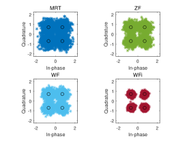
(a) ${\eta=0,N=32,M=4}$

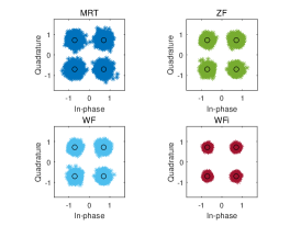
(b) ${\eta=0,N=128,M=4}$

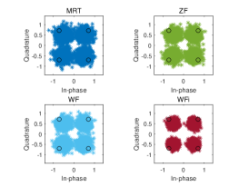
(c) ${\eta=0.36,N=128,M=4}$

Figure 1: The estimated outputs for QPSK signaling as a function of CSI-related parameter $\eta$ and system size ($N$ receive antennas and $M$ UEs), at an SNR level of 5dB.

II-B Quantized Precoding Problem Formulation with Imperfect CSI

In previous studies, it is commonly assumed that the CSI is perfectly known, i.e., ${\bf{\widetilde{H}}}={\bf{H}}$. However, in practical applications, the CSI is inevitably contaminated by noise. In this paper, we follow [23, 33] for a model of imperfect CSI through a Gauss-Markov uncertainty of the form

$${\bf{\widetilde{H}}}=\sqrt{1-\eta}{\bf{H}}+\sqrt{\eta}{\bf{E}},$$ (4)

where ${{\bf{\widetilde{H}}}}$ is the imperfect observation of channel available to the BS and $\bf{E}$ is modeled as AWGN. The CSI-related parameter $\eta$ characterizes the partial CSI. Specifically, $\eta=0$ means perfect CSI, the values of $0<\eta<1$ correspond to partial CSI and $\eta=1$ accounts for no CSI. In this work, the parameter $\eta$ is restricted to $0\leq\eta<1$.

In the case of imperfect CSI, the quantized precoding problem can be formulated as [23]

$$\begin{array}[]{*{20}{c}}{\mathop{{\rm{minimize}}}\limits_{\beta\in{\mathbb{R}^{+}}}}&{\left\|{{\bf{s}}-\beta{\bf{\widetilde{H}}}Q\left({\bf{x}}\right)}\right\|_{2}^{2}+{\beta^{2}}M{\sigma^{2}}}\\ {{\rm{s}}.{\rm{t}}.}&{E\left\{{{{\bf{z}}^{\rm{H}}}{\bf{z}}}\right\}\leq P_{TX}}\end{array}.$$ (5)

We end this part by providing some technical explanations of the model used in (4). It has shown in numerous studies [28, 23, 33, 26, 39, 40, 41] that (4) is a widely model to study specific scenarios of the imperfect CSI. The parameter $\beta$ is a function of system parameters depending in different scenarios. For example, with minimum mean-square error channel estimation, $\beta$ represents a function of pilot symbol SNR [39]. For an analog feedback link, $\beta$ is a function of the number of the coefficient of the employed channel and the SNR of the feedback link [40]. Recently, $\beta$ is used to concentrate the differences between the uplink and the downlink SNRs [41]. In this paper, we restrict our choice of $\beta$ to a constant value but one can extend the results to being an arbitrary function of the system parameters or investigate the outdated channel state information [42].

II-C Why should we need robust precoding for coarsely quantized massive MU-MIMO system?

For the massive MU-MIMO downlink, there is a growing concern on the excessive energy consumption, which is mainly caused by the data converters at the BS [1]. Equipping the BS with low-resolution DACs (i.e., 1-bit to 4-bit) has been proven to be a potential way to reduce power consumption. Under the assumption of perfect CSI, many studies show that the use of low-resolution DACs could greatly reduce the power consumption while keeping the performance loss within tolerable levels. However, CSI errors are inevitable in practice.

Fig. 1 shows the experimental result of the estimated outputs of the MU-MIMO system with 1-bit DACs. Three quantized linear precoding schemes (MRT, ZF, WF,) are employed. Specially, the notation WFi is referred to the case of WF precoding with infinite-resolution DACs. In the case of perfect CSI, it is observed from Fig. 1a and Fig. 1b that the QPSK constellation becomes more distinguishable with increasing the number of transmit antennas, yielding better BER performance of all precoders. However, Fig. 1b and Fig. 1c illustrate that the precoding schemes for the MU-MIMO system with low-resolution DACs are more susceptible to CSI errors than that with ideal DACs. In addition, increasing the number of transmit antennas are insufficient in general for securing the BER performance of the coarsely-quantized MU-MIMO systems with imperfect channel knowledge.

The observations described above motivated us to develop a new method for the quantized precoding problem taking into account the CSI errors.

II-D Linearized Analysis and Problem Decomposition

It has been mentioned in Section I and Section II-B that there is no available robust algorithm directly applies to solve the quantized precoding problem (5), which are mainly due to two factors: 1) The nonlinearity of ${\bf x}$ and ${\bf z}$; 2) Imperfect CSI. In what follows, a linearized analysis of (2) is firstly given to ameliorate the nonlinearity difficulties. Based on the linearized analysis, the original quantized precoding problem is then decomposed into three sub-problems, which are sub-sequently solved.

The proposed algorithm in this paper takes advantage of the Bussgang theorem, and is applicable for any linear precoding scheme, e.g., MRT, ZF, WF, and WFQ [43]. In what follows, we examine, in detail, the special case of the WF precoder.

Let ${{\bf{\widetilde{P}}}}$ be a linear precoding matrix. By taking the advantage of the well-known Bussgang theorem [35], one can obtain

$${\bf{z}}=Q\left({\bf{x}}\right)=Q\left({{\bf{{{\bf{\widetilde{P}}}}s}}}\right)={\bf{\widetilde{F}{{\bf{\widetilde{P}}}}s}}+{\bf{d}}.$$ (6)

Plugging (6) into (5) and applying the Lagrangian multiplier method [4], one can get the quantized WF precoding matrix as:

$${\bf{P}}^{WF} =\widetilde{\beta}^{WF}{\bf{\widetilde{F}}}{\bf{\mathord{\buildrel{\lower 3.0pt\hbox{$\scriptscriptstyle\smile$}}\over{P}}}},$$ (7)

$${\bf{\mathord{\buildrel{\lower 3.0pt\hbox{$\scriptscriptstyle\smile$}}\over{P}}}} ={{{\bf{\widetilde{H}}}}^{\rm{H}}}{\left({{\bf{\widetilde{H}}}{{{\bf{\widetilde{H}}}}^{\rm{H}}}+M{\bf\theta}}\right)^{-1}},$$

$$\widetilde{\beta}^{WF} =\frac{1}{{\sqrt{P}}}{\mathop{\rm tr}\nolimits}{\left({{{{\bf{\mathord{\buildrel{\lower 3.0pt\hbox{$\scriptscriptstyle\smile$}}\over{P}}}}}^{\rm{H}}}{\bf{\mathord{\buildrel{\lower 3.0pt\hbox{$\scriptscriptstyle\smile$}}\over{P}}}}}\right)^{-1/2}},$$

$${\bf\theta} =(\sigma^{2}{\bf{I}}+\sigma_{\bf{d}}^{2}),$$

$$\sigma_{\bf{d}}^{2} =\left({1-{\rm{diag}}\left({{\bf{\widetilde{F}}}}\right)}\right)\left({M{\sigma^{2}}+1}\right).$$

With results in (7), the original precoding problem now can be decomposed into three subproblems: a) Estimation of the CSI-related parameter $\eta$; b) Reconstruction of CSI ${\bf{H}}$ from the noisy observation ${\bf{\widetilde{H}}}$; c) Estimation of the coefficients matrix $\bf{F}$ under imperfect CSI. The solutions for all the three subproblems are fundamentally based on the block random matrix theory [36], which is presented in details in the following.

III The Proposed Solution: The Eigen-Inference Precoder

We first provide a sketch of the algorithm development in the following. Firstly, we present some theoretical basics from random matrix theory that will be needed in the ensuing analysis. The main metrics we employ are introduced and some favorable properties are shown in detail. Secondly, to estimate the CSI-related parameter $\eta$, an EI-based moments matching method is then proposed. Furthermore, following the strategies in [44, 45], an EI-based rotation invariant estimator for constructing the estimation of cleaned CSI ${{\bf{\hat{H}}}}$ is developed. Lastly, with the refined CSI, the desired precoding matrix, the cleaned precoding factor, and the estimate of the coefficient matrix $\bf{\hat{F}}$ are accordingly obtained.

III-A Random Matrix Basics and Main Metrics

We start by presenting some basics from random matrix theory that will be needed in the following algorithm development. For a square random matrix ${\bf{A}}\in{\mathbb{C}}^{M\times M}$, the resolvent of ${\bf{A}}$ is defined as

$${{\bf{G}}_{\bf{A}}}\left(z\right)={\left({z{{\bf{I}}_{M}}-{\bf{A}}}\right)^{-1}}.$$ (8)

The normalized trace of (8) gives

$${\mathfrak{g}}_{\bf{A}}^{M}\left(z\right)=\frac{1}{M}{\mathop{\rm tr}\nolimits}\left[{{{\bf{G}}_{\bf{A}}}\left(z\right)}\right].$$

In the limit of large dimension, one has ${\mathfrak{g}}_{\bf{A}}^{M}\left(z\right)\mathop{\rightarrow}\limits_{M\to\infty}{{\mathfrak{g}}_{\bf{A}}}\left(z\right)$, where ${{\mathfrak{g}}_{\bf{A}}}\left(z\right)$ is the $Stieltjes$ transform of ${\bf{A}}$. The asymptotic empirical distribution of eigenvalues ${F_{\bf{A}}}\left(\lambda\right)$ (with density ${\rho_{\bf{A}}\left(\lambda\right)}$) can be described in terms of its $Stieltjes$ transform [22], defined by

$${{\mathfrak{g}}_{{\bf{A}}}}\left(z\right)=\int{\frac{{d{F_{\bf{A}}}\left(\lambda\right)}}{{\lambda-z}}}=\int{\frac{{\rho_{\bf{A}}\left(\lambda\right)}}{{\lambda-z}}d\lambda}.$$ (9)

Besides, the $R$ transform, a handy transform which enables the characterization of the limiting eigen-spectra of a sum of free random matrices from their individual limiting eigen-spectra, can be defined as

$${R_{\bf{A}}}\left(z\right)={\mathfrak{g}}_{\bf{A}}^{-1}\left(z\right)-\frac{1}{z}.$$ (10)

Furthermore, the $R$ transform can be expanded as [46]:

$${R_{\bf{A}}}\left(z\right)=\sum\limits_{l=1}^{\infty}{{\kappa_{l}}}\left({\bf{A}}\right){z^{l-1}},$$ (11)

where ${\kappa_{l}}\left({\bf{A}}\right)$ denotes the so-called $free\ cumulant$ which can be expressed as a function of moments of ${\bf{A}}$. Specially, given the $m$-th moments of $\bf{A}$ (denoted by $\varphi\left({{{\bf{A}}^{k}}}\right)$) and using the so-called cumulant formula [46], one can have

$$\varphi\left({{{\bf{A}}^{m}}}\right)=\sum\limits_{l=1}^{m}{{\kappa_{l}}\left({{{\bf{A}}^{m}}}\right)\sum\limits_{{m_{1}},\cdots,{m_{l}}}{\varphi\left({{{\bf{A}}^{{m_{1}}-1}}}\right)\cdots\varphi\left({{{\bf{A}}^{{m_{l}}-1}}}\right)}},$$ (12)

where, for ${k=1,\cdots,l}$, ${m_{k}}$ is a non-negative integer and satisfies ${m_{1}}+...+{m_{l}}=m$. For completeness, the first three cumulants are given by

$${\kappa_{1}}={\varphi_{1}},\ {\kappa_{2}}={\varphi_{2}}-\varphi_{1}^{2},\ {\kappa_{3}}={\varphi_{3}}-3{\varphi_{2}}{\varphi_{1}}+2\varphi_{1}^{2},$$ (13)

where we denote $\varphi\left({{{\bf{A}}^{k}}}\right)$ as ${\varphi_{k}}$ for simplicity.

It is noted that, in our case, ${\bf{H}}\in{\mathbb{C}^{M\times N}}$ is a rectangular random matrix, having complex-valued eigenvalues and eigenvectors. The well-known Hermitian random matrix theory can not be applied unless a proper strategy is used. In this paper, our analysis is based on BSCA and the noisy observation of BSCA, of forms

$${\bf{B}}=\left[{\begin{array}[]{*{20}{c}}{\bf{0}}&{\bf{H}}\\ {{{\bf{H}}^{\mathop{\rm H}\nolimits}}}&{\bf{0}}\end{array}}\right],$$ (14)

and

$${\bf{\widetilde{B}}}=\left[{\begin{array}[]{*{20}{c}}{\bf{0}}&{{\bf{\widetilde{H}}}}\\ {{{{\bf{\widetilde{H}}}}^{\rm{H}}}}&{\bf{0}}\end{array}}\right]={\bf{B}}+\alpha\left[{\begin{array}[]{*{20}{c}}{\bf{0}}&{\bf{E}}\\ {{{\bf{E}}^{\rm{H}}}}&{\bf{0}}\end{array}}\right]={\bf{B}}+{\bf{\widetilde{E}}},$$ (15)

where $\alpha=\sqrt{\eta/\left({1-\eta}\right)}$. The observations in (14) and (15) are known as the Girko’s Hermitization trick [47, 48], which has been widely used in the case of theoretical analysis of Hermitian random matrix. In this paper, the rectangular random matrix is considered. Thanks to the Girko’s Hermitization trick, the theoretical analysis developed in this paper is based on the spectral theory of block Hermitian random matrices, instead of the much involved spectral theory of rectangular random matrices.

We, in particular, are aiming to build the connection between the limiting spectra distribution (LSD) of ${\bf{B}}$ and ${\bf{\widetilde{B}}}$. Let us define two more auxiliary matrices:

$${\bf{D}}={\bf{B}}{{\bf{B}}^{\rm H}}=\left[{\begin{array}[]{*{20}{c}}{{\bf{H}}{{\bf{H}}^{\rm H}}}&0\\ 0&{{{\bf{H}}^{\rm H}}{\bf{H}}}\end{array}}\right],$$ (16)

and

$${\bf{\widetilde{D}}}={\bf{\widetilde{B}}}{{{\bf{\widetilde{B}}}}^{\rm H}}=\left[{\begin{array}[]{*{20}{c}}{{\bf{\widetilde{H}}}{{\bf{\widetilde{H}}}^{\rm H}}}&0\\ 0&{{\bf{\widetilde{H}}}{{\bf{\widetilde{H}}}^{\rm H}}}\end{array}}\right].$$ (17)

With notations in (14)-(17), one can find that a direct relationship among eigenvalues of $\bf{B}$ (or ${\bf{\widetilde{B}}}$), $\bf{D}$ (or ${\bf{\widetilde{D}}}$) and ${{\bf{H}}{{\bf{H}}^{\rm H}}}$ (or ${{\bf{\widetilde{H}}}{{\bf{\widetilde{H}}}^{\rm H}}}$), which can be expressed as

$${\lambda^{\bf{D}}}=\left\{{\begin{array}[]{*{20}{c}}{{\lambda^{{\bf{H}}{{\bf{H}}^{\rm H}}}},}&{{\lambda^{\bf{D}}}\neq 0}\\ {0,}&{{\lambda^{\bf{D}}}=0}\end{array}}\right.,\ {\lambda^{\bf{B}}}=\pm\sqrt{{\lambda^{\bf{D}}}},$$ (18)

and

$${\lambda^{\bf{\widetilde{D}}}}=\left\{{\begin{array}[]{*{20}{c}}{{\lambda^{{\bf{\widetilde{H}}}{{\bf{\widetilde{H}}}^{\rm H}}}},}&{{\lambda^{\bf{\widetilde{D}}}}\neq 0}\\ {0,}&{{\lambda^{\bf{\widetilde{D}}}}=0}\end{array}}\right.,\ {\lambda^{\bf{\widetilde{B}}}}=\pm\sqrt{{\lambda^{\bf{\widetilde{D}}}}}.$$ (19)

Besides, the limiting spectra connection between the noisy BSCA and the true BSCA can be expressed as in the following results.

Lemma III.1.

For the BSCA ${\bf{B}}$ defined in (14), the $Stieltjes$ transform of the LSD of ${\bf{H}}{{{\bf{H}}}^{\rm H}}$ can be represented by the $Stieltjes$ transform of the LSD of ${\bf{B}}$ as:

$${{\mathfrak{g}}_{{\bf{H}}{{\bf{H}}^{H}}}}\left(z\right)=\frac{{q+1}}{{2q}}{{\mathfrak{g}}_{\bf{D}}}\left(z\right)-\frac{{q-1}}{{2q}}\frac{1}{z}$$ (20)

Lemma III.1 bridges up the LSD connections between the interested block random matrix ${\bf{D}}$ and ${{\bf{H}}{{\bf{H}}^{\rm H}}}$, whose density is subject to the well-known Marchenko-Pastur law.

Lemma III.2.

Let $q=M/N<1$. For the BSCA ${\bf{B}}$ and the sample covariance of the BSCA ${\bf{D}}$, the $Stieltjes$ transforms of the LSDs of ${\bf{B}}$ and ${\bf{D}}$ satisfy

$${{\mathfrak{g}}_{\bf{B}}}\left(z\right)=z{{\mathfrak{g}}_{\bf{D}}}\left({{z^{2}}}\right).$$ (21)

Lemma III.3.

Let the random matrices ${\bf{D}}$ and ${\bf{B}}$ be defined as in Lemma III.2. The $S$ transforms of the LSDs of ${\bf{B}}$ and ${\bf{D}}$ meet

$${\left[{{S_{\bf{B}}}\left(z\right)}\right]^{2}}=\frac{{1+z}}{z}{S_{\bf{D}}}\left(z\right).$$ (22)

Lemma III.2 and Lemma III.3 state direct LSD linkage between ${\bf{B}}$ and ${\bf{D}}$. The proof of the above lemmas are respectively deferred to Appendix A, Appendix B, and Appendix C. With the technical results shown in Lemma III.1, Lemma III.2 and Lemma III.3, the statistical properties (i.e., the asymptotic empirical distribution of eigenvalues) of ${\bf{B}}$ can be obtained by the well-established Hermitian random matrix theory. Besides, combined with the addition law [46, 49]:

$${R_{{\bf{X}}+{\bf{Y}}}}\left(z\right)={R_{\bf{X}}}\left(z\right)+{R_{\bf{Y}}}\left(z\right),$$ (23)

one can reveal the limiting spectra connection between the noisy BSCA and the true BSCA.

All technical results shown above act as fundamental roles which enable us to tackle the quantized precoding problem introduced in Section II-B. The detailed analysis is given in the following.

III-B Determination of the Unknown Parameter $\eta$: An EI-based Moments Matching Algorithm

In this part, we propose a moments matching algorithm to determinate the unknown parameter $\eta$ in (4). Our analysis is based on the free probability which is a powerful tool for analyzing the eigen-spectra of large random matrices. The proposed moments matching algorithm can provide a robust and flexible estimation of $\eta$ without specifying an explicit relationship between the number of UEs and the number of antennas.

The estimation of $\eta$ is enabled by random matrix theory which offers a collection of useful results on the asymptotic behavior of the BSCA $\bf{B}$ and its noisy observation ${\bf{\widetilde{B}}}$, which are shown in the following theoretical results.

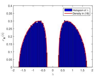
Figure 2: The empirical distribution of the nonzero eigenvalues of BSCA: $M=128$, $N=256$, $q=0.5$.

Theorem III.1.

For the BSCA $\bf{B}$ defined in (14), the empirical distribution of the eigenvalues of $\bf{B}$ converges almost surely, as $M,N\rightarrow\infty$ with $M/N\rightarrow q$, to a nonrandom distribution whose density function is

$${\rho_{\bf{B}}}\left(x\right)=\frac{{\sqrt{\left({{b^{2}}-{x^{2}}}\right)\left({{x^{2}}-{a^{2}}}\right)}}}{{\left({q+1}\right)\pi\left|x\right|}}+\frac{{1-q}}{{1+q}}\delta\left(x\right),$$ (24)

where $a\leq\left|x\right|\leq b$ and

$$a=1-\sqrt{q},b=1+\sqrt{q}.$$

The proof of Theorem III.1 is deferred to Appendix D. As an illustration of the result obtained in Theorem III.1, Fig. 2 shows the empirical distribution of the nonzero eigenvalues of the BSCA. it can been seen that the empirical density function (24) agrees well with the simulation result.

Combined with the favorable results given in Theorem III.1, Lemma III.2, Lemma III.3 and Lemma III.1, one can obtain the following result for the sample covariance of the noisy channel matrix.

Theorem III.2.

For the noisy channel matrix ${\bf{\widetilde{H}}}\in{\mathbb{C}}^{M\times N}$, the empirical distribution of eigenvalues of its sample covariance matrix ${{\bf{\widetilde{H}}}{{\bf{\widetilde{H}}}^{\rm H}}}$ converges almost surely to a limit distribution whose $Stieltjes$ transform , denoted by $G={{\mathfrak{g}}_{{\bf{\widetilde{H}}}{{\bf{\widetilde{H}}}^{\rm H}}}}\left(z\right)$, satisfies

$${\rm{-2}}Gz+{G^{2}}\left({1+{k^{2}}}\right)qz+h\left(G\right)=0,$$ (25)

as $M,N\to\infty$ with the ratio $q=M/N<1$ fixed, and

$$h\left(G\right) =\sqrt{1+{G^{2}}z\left({4+q\left({-2+{G^{2}}qz}\right)}\right)}$$

$$+\sqrt{1+{G^{2}}{\alpha^{2}}z\left({4+q\left({-2+{G^{2}}z{\alpha^{2}}q}\right)}\right)}.$$

The proof of Theorem III.2 is deferred to Appendix E. Combined the theoretical result in Theorem III.2 with the relation in (10), we can obtain the $R$ transform of ${{\bf{\widetilde{H}}}{{\bf{\widetilde{H}}}^{\rm H}}}$. Accordingly, we can infer the parameters of the underlying noisy channel matrix ${\bf{\widetilde{H}}}$ from a realization of its sample covariance matrix. Taking Taylor’s expansion for the obtained $R$ transform, the first three moments of the sample covariance matrix can be analytically parameterized by the unknown parameters $\eta$ of form:

$$\varphi\left({{\bf{\widetilde{H}}}{{\bf{\widetilde{H}}}^{\rm H}}}\right) =\frac{1}{{1-\eta}},$$ (26)

$$\varphi\left[{{{\left({{{\bf{\widetilde{H}}}{{\bf{\widetilde{H}}}^{\rm H}}}}\right)}^{2}}}\right] =\frac{{2\left({1-\eta}\right){\eta}\left({1-q}\right)+q}}{{{{\left({1-\eta}\right)}^{2}}}},$$ (27)

$$\varphi\left[{{{\left({{{\bf{\widetilde{H}}}{{\bf{\widetilde{H}}}^{\rm H}}}}\right)}^{3}}}\right] =\frac{{q\left({3\left({1-\eta}\right){\eta}\left({1-q}\right)+q}\right)}}{{{{\left({1-\eta}\right)}^{3}}}}.$$ (28)

Given an observation ${\bf{\widetilde{H}}}$, we can compute estimates of the first three moments of its sample covariance matrix as [46]

$$\hat{\varphi}\left[{{{\left({{{\bf{\widetilde{H}}}{{\bf{\widetilde{H}}}^{\rm H}}}}\right)}^{k}}}\right]=\frac{1}{M}{\mathop{\rm tr}\nolimits}\left[{{{\left({{{\bf{\widetilde{H}}}{{\bf{\widetilde{H}}}^{\rm H}}}}\right)}^{k}}}\right],$$ (29)

for $k=1,2,3.$ Since $q=N/M$ is already known, we can estimate the CSI-related parameter ${\eta}$ by EI-based $moments\ matching$, in particular, by solving the non-linear system of equations:

$$\hat{\alpha}=\mathop{{\mathop{\rm argmin}\nolimits}}\limits_{\alpha>0}{\left\|{\sum\limits_{k=1}^{3}{\hat{\varphi}\left[{{{\left({{{\bf{\widetilde{H}}}{{\bf{\widetilde{H}}}^{\rm H}}}}\right)}^{k}}}\right]-\varphi\left[{{{\left({{{\bf{\widetilde{H}}}{{\bf{\widetilde{H}}}^{\rm H}}}}\right)}^{k}}}\right]}}\right\|^{2}}.$$ (30)

Though the EI-based moments matching algorithm described above is theoretically exact when $M,N\rightarrow\infty$, we verify through various simulations that the proposed method is sufficiently accurate for even small values of $N$ and $M$ (i.e., $M=8$, $N=32$). See experimental results in Section IV for more details.

III-C CSI Cleaning Based on Random Matrix Theory: EI-based Rotation Invariant Estimation

We now attempt to construct an estimator ${{\bf{\hat{H}}}}$ of the true channel matrix ${\bf{H}}$ that relies on the imperfect observation ${{\bf{\widetilde{H}}}}$. We will focus on the case that ${\bf{H}}$ is an $M\times N$ random matrix that ${M,N}\to\infty$ with the ratio $q=M/N<1$ fixed. Our analysis is based on the rotation invariant estimation theory [50, 44, 45] and by leveraging spectral properties of the BSCA (shown in Section III-A).

Let ${\lambda_{1}}\geq\cdots\geq{\lambda_{M+N}}$ and ${{\bf{u}}_{1}},\cdots,{{\bf{u}}_{M+N}}$ be the eigenvalues and eigenvectors of a true matrix (denoted by $\bf{A}$), respectively. For the noisy matrix (denoted by ${\bf{\widetilde{A}}}$), its eigenvalues and eigenvectors are respectively denoted by ${\omega_{1}}\geq\cdots\geq{\omega_{M+N}}$ and ${{\bf{v}}_{1}},\cdots,{{\bf{v}}_{M+N}}$.

Based on the minimum mean-square error (MMSE) criterion [51], one can obtain the optimal estimate of $\bf{A}$ by solving

$${\bf{\hat{A}}}=\mathop{\arg{\rm{minimize}}}\limits_{\Omega({\bf{\tilde{A}}})}\left\|{\Omega({\bf{\tilde{A}}})-{\bf{A}}}\right\|_{\rm{F}}^{2}.$$ (31)

In this paper, we use ${\Omega({\bf{\tilde{A}}})}$ to denote the set of all possible rotation invariant estimators. In statistics (see the tutorial work of [44] for more details.), any rotation invariant estimator $\Omega\left({\bf{A}}\right)$ enjoys the same eigenvectors as the perturbed matrix ${\bf{\widetilde{A}}}$ . In other words, we can have

$$\Omega\left({\bf{A}}\right)=\sum\limits_{k=1}^{M+N}{{\xi_{k}}{{\bf{v}}_{k}}{\bf{v}}_{k}^{\mathop{\rm H}\nolimits}},$$ (32)

where ${\xi_{1}},\cdots,{\xi_{M+N}}$ are quantities to be determined. Using the fact that $\left\|{\bf{W}}\right\|_{\mathop{\rm F}\nolimits}^{2}={\mathop{\rm tr}\nolimits}\left({{\bf{W}}{{\bf{W}}^{\rm{H}}}}\right)$, one can have

$$\left\|{\Omega({\bf{\tilde{A}}})-{\bf{A}}}\right\|_{\rm{F}}^{2}={\bf{tr}}{\left({\sum\limits_{k=1}^{M+N}{{\xi_{k}}{{\bf{v}}_{k}}{\bf{v}}_{k}^{\rm{H}}-\sum\limits_{k=1}^{M+N}{{\lambda_{k}}{{\bf{u}}_{k}}{\bf{u}}_{k}^{\rm{H}}}}}\right)^{2}}.$$ (33)

Since ${\xi_{k}},k=1,\cdots,M+N$ are quadratic in (33), substituting (32) into (31) gives the optimal solution of (31):

$${\bf{\hat{A}}}=\sum\limits_{k=1}^{M+N}{{\hat{\xi}_{k}}{{\bf{v}}_{k}}{\bf{v}}_{k}^{\mathop{\rm H}\nolimits}},$$ (34)

and

$${{\hat{\xi}}_{k}}=\sum\limits_{j=1}^{M+N}{{\lambda_{j}}{{\left({{\bf{u}}_{j}^{\rm{H}}{{\bf{v}}_{k}}}\right)}^{2}}}.$$ (35)

In the limit of large dimensions [52], ${{\hat{\xi}}_{k}}$ can be approximately calculated by its expectation value

$${{\hat{\xi}}_{k}}=\sum\limits_{j=1}^{M+N}{{\lambda_{j}}\mathbb{E}\left[{{{\left({{\bf{u}}_{j}^{\rm{H}}{{\bf{v}}_{k}}}\right)}^{2}}}\right]}.$$

In particular, let ${\bf{\widetilde{A}}}={{\bf{\widetilde{H}}}{{\bf{\widetilde{H}}}^{\rm H}}}/\left({1-\eta}\right)$, based on rigorous mathematical derivation, one can obtain the estimates of the true eigenvalues of ${\bf A}={{{\bf{H}}^{\rm H}}{\bf{H}}}$ by [45]

$${{\hat{\lambda}}_{k}}={\phi_{1}}\left({{\omega_{k}}}\right){\phi_{2}}\left({{\omega_{k}}}\right)+{\phi_{3}}\left({{\omega_{k}}}\right),$$ (36)

where

$${\phi_{1}}\left({{\omega_{k}}}\right) =1-q{\alpha^{2}}{h_{k}},\alpha=\sqrt{\eta/\left({1-\eta}\right)},$$

$${\phi_{2}}\left({{\omega_{k}}}\right) ={{\omega_{k}}-{\alpha^{2}}\left({1-q}\right)-2q{\alpha^{2}}{h_{k}}},$$

$${\phi_{3}}\left({{\omega_{k}}}\right) ={h_{k}}\left({{\omega_{k}}-{\alpha^{2}}\left({1-q}\right)+q{\alpha^{2}}{\omega_{k}}\left({{\rho_{k}}-{h_{k}}}\right)}\right),$$

$${\rho_{k}} =\mathop{\lim}\limits_{{\epsilon_{k}}\to{0^{+}}}{\mathop{\Im}\nolimits}\left[{{\mathfrak{g}_{\bf{A}}}\left({{\omega_{k}}+{\mathop{\rm i}\nolimits}{\epsilon_{k}}}\right)}\right],$$

$${h_{k}} =\mathop{\lim}\limits_{{\epsilon_{k}}\to{0^{+}}}{\mathop{\Re}\nolimits}\left[{{\mathfrak{g}_{\bf{A}}}\left({{\omega_{k}}+{\mathop{\rm i}\nolimits}{\epsilon_{k}}}\right)}\right].$$

With (36) and the direct relation shown in (18) and (19), one can get the estimates of the eigenvalues of $\bf{D}$ and $\bf{B}$. With (34), we can obtain the estimates of $\bf{D}$ and $\bf{B}$ (denoted by $\bf{\hat{B}}$). Finally, the estimate of the true channel matrix is the upper nonzero block of $\bf{\hat{B}}$.

The results in (36) have been proven by means of the Replica method [44, 45] in the case of the Hermitian random matrix. The analysis performed above is based on the theoretical work of [44, 45]. Our contributions are:1) We develop an EI-based moments matching method to estimate the CSI-related parameter $\eta$, which is actually unknown in practice. 2) We propose a theoretically simple approach to derive the estimator of the $Stieltjes$ transform of ${\bf{\widetilde{A}}}$ (denoted by ${\mathfrak{g}_{\bf{A}}}(z)$) in Theorem III.2, which is useful in (36).

III-D Determination of the Coefficient Matrix $\bf{F}$

With cleaned CSI, we are now ready to determine $\bf{F}$. It has been widely assumed that the elements of the uniform quantization errors $\bf{d}$ converge in distribution to a zero-mean Gaussian random variable, whose variance can be characterized in closed form. Indeed, such an assumption is essentially valid when the errors from individual channels are asymptotically pairwise independent, each uniformly distributed within the quantization thresholds [53]. Denote the estimated precoding matrix by ${\bf{\hat{P}}}$. With Gaussian assumption of ${\bf{d}}$ and based the Bussgang theorem, one can estimate $\bf{F}$ by minimzing the square error

$$\mathbb{E}\left\|{\bf{d}}\right\|_{2}^{2}=\mathbb{E}\left\|{{\bf{x}}-{\bf{Fz}}}\right\|_{2}^{2},$$ (37)

where ${\bf z}={\bf{\hat{P}}s}$. Then

$$\begin{array}[]{l}\begin{aligned} {\bf{\hat{F}}}&=\mathop{\arg{\rm minimize}}\limits_{\bf{F}}\mathbb{E}\left\|{{\bf{x}}-{\bf{Fz}}}\right\|_{2}^{2}\\ &=\mathop{\arg{\rm minimize}}\limits_{\bf{F}}{\rm{tr}}\left({{{\bf{R}}_{{\bf{xx}}}}-{{\bf{R}}_{{\bf{xz}}}}{{\bf{F}}^{\rm{H}}}-{\bf{F}}{{\bf{R}}_{{\bf{zx}}}}+{\bf{F}}{{\bf{R}}_{{\bf{zz}}}}{{\bf{F}}^{\rm{H}}}}\right)\\ &=\mathop{\arg{\rm minimize}}\limits_{\bf{F}}f\left({\bf{F}}\right),\end{aligned}\end{array}$$ (38)

can be obtained. A solution of (38) has to satisfy

$$\frac{{\partial f\left({\bf{F}}\right)}}{{\partial{\bf{F}}}}=-2{{\bf{R}}_{{\bf{xz}}}}+2{\bf{F}}{{\bf{R}}_{{\bf{zz}}}},$$ (39)

which yields

$${\bf{\hat{F}}}={{\bf{R}}_{{\bf{xz}}}}{\bf{R}}_{{\bf{zz}}}^{-1},$$ (40)

where

$${{\bf{R}}_{{\bf{zz}}}}={\mathbb{E}_{\bf{s}}}\left[{{\bf{z}}{{\bf{z}}^{\rm{H}}}}\right]={\bf{\hat{P}}}{\mathbb{E}_{\bf{s}}}\left[{{\bf{s}}{{\bf{s}}^{\rm{H}}}}\right]{{\bf{\hat{P}}}^{\rm{H}}}={\bf{\hat{P}}}{{\bf{\hat{P}}}^{\rm{H}}},$$ (41)

and

$${{\bf{R}}_{{\bf{xz}}}}={\mathbb{E}_{\bf{s}}}\left[{{\bf{x}}{{\bf{z}}^{\rm{H}}}}\right]={\mathbb{E}_{\bf{s}}}\left[{Q\left({\bf{z}}\right){{\bf{z}}^{\rm{H}}}}\right].$$ (42)

It is assumed that $\bf{F}$ is a diagonal matrix, then we can obtain its diagonal elements

$${\left[{{\bf{\hat{F}}}}\right]_{m,m}}=\frac{{{E_{x}}\left[{Q\left(x\right){x^{*}}}\right]}}{{\sigma_{m}^{2}}},$$ (43)

where $m=1,2,\cdots M$ and $\sigma_{m}^{2}={\left[{{{\bf{R}}_{{\bf{zz}}}}}\right]_{m,m}}$.

Let

$${l_{b}}=\Delta\left({b-\frac{{{2^{B}}-1}}{2}}\right),\ b=1,\cdots,{2^{B}-1}\ ,$$

and

$${\tau_{b}}=\Delta\left({b-{2^{B-1}}}\right),\ b=2,\cdots,{2^{B}}\ ,$$

respectively be the quantization labels and quantization thresholds of a $B$ bit uniform quantizer, whose output can be expressed as

$$Q\left(z\right)=\frac{\Delta}{2}\left({1-{2^{B}}}\right)+\Delta\sum\limits_{l=1}^{{2^{B}}-1}{{\delta_{\left[{\Delta\left({l-{2^{B-1}}}\right),\left.\infty\right)}\right.}}\left(z\right)},$$ (44)

where $\delta_{\Phi}\left({x}\right)$ is an indicator function defined as

$${\delta_{\Theta}}\left(x\right)=\left\{{\begin{array}[]{*{20}{c}}1&{{\rm{if}\ }x\in\Theta}\\ 0&{{\rm{if}\ }x\notin\Theta}\end{array}}\right..$$

Substituting (44) into (43) gives

$$\begin{array}[]{c}\begin{aligned} {\left[{{\bf{\hat{F}}}}\right]_{m,m}}&=\frac{\Delta}{{\sigma_{u}^{2}/2}}\sum\limits_{l=1}^{{2^{B}}-1}{\int_{l-{2^{B-1}}}^{\infty}{\frac{x}{{\sqrt{\pi\sigma_{u}^{2}}}}\exp\left({-\frac{{{x^{2}}}}{{\sigma_{u}^{2}}}}\right)dx}}\\ &=\frac{\Delta}{{\sqrt{\pi\sigma_{u}^{2}}}}\sum\limits_{l=1}^{{2^{B}}-1}{\exp\left({-\frac{{{\Delta^{2}}}}{{\sigma_{u}^{2}}}{{\left({l-{2^{B-1}}}\right)}^{2}}}\right)}\end{aligned}\end{array}.$$ (45)

So far, the quantized precoding problem has been tackled. The proposed EI precoder is summarized in Algorithm 1.

Algorithm 1 The Proposed EI Precoding Algorithm

1:  $\bf{Input:}$ Imperfect SCM of CSI: ${\bf{\widetilde{H}}}$.

2:  Construct noisy BSCA ${\bf{\widetilde{B}}}$ using (15).

3:  Calculate the estimates of the first three moments of ${{\bf{\widetilde{H}}}{{\bf{\widetilde{H}}}^{\rm H}}}$ using (29) and compute the related moments using (13).

4:  Substituting the obtained moments $\hat{\varphi}\left[{{{\left({{{\bf{\widetilde{H}}}{{\bf{\widetilde{H}}}^{\rm H}}}}\right)}^{k}}}\right]$ into (30) to estimate the CSI-related parameter ${\hat{\eta}}$.

5:  Performing eigenvalue decomposition of ${\bf{\widetilde{B}}}$ yields

$$\left[{{\bf{U}},{\bf{S}}}\right]={\mathop{\rm eig}\nolimits}\left({\bf{\widetilde{B}}}\right).$$

6:  Combined with the CSI-related parameter ${\hat{\eta}}$, calculating the estimates of eigenvalues of ${\bf{B}}$ using (19) and (36) gives $\hat{\bf{S}}$.

7:  Reconstructing ${\bf{B}}$ as

$${\bf{\hat{B}}}={{{\bf{U}}\hat{\bf{S}}}}{{\bf{U}}^{\rm{H}}}.$$

The estimated CSI, denoted by ${\bf{\hat{H}}}$, is the upper triangular part of ${\bf{\hat{B}}}$ and ${\bf{\hat{H}}}={{{\bf{\hat{B}}}}_{1:M,M+1:M+N}}$.

8:  Plugging the estimated CSI ${\bf{\hat{H}}}$ into (7) yields the estimates of the precoding matrix and precoding factor, which are denoted by $\bf{\hat{P}}$ and $\bf{\hat{\beta}}$, respectively.

9:  Calculating the estimate of the coefficients matrix $\bf{F}$ using (45) to obtain $\bf{\hat{F}}$.

10:  $\bf{Output:}$ $\bf{\hat{P}}$, $\bf{\hat{F}}$, and $\bf{\hat{\beta}}$.

III-E Complexity Analysis

We now analyze the computational complexity of the proposed algorithms (Algorithm 1). In step 3 of Algorithm 1, computing the first three moments has a complexity of $O\left(k_{1}MN^{2}\right)$, which involves the cost of $k_{1}$ matrix multiplications. Step 4 of Algorithm 1 is the linear square problem with a closed form solution in the form of pseudoinverse, which yields complexity of $O\left(K^{w}\right)$ ($K$ is the number of the unknown parameter and $w$ satisfies $w<2.37$ [55]). The complexity of the eigenvalue decomposition in Step 5 is $O\left(M^{3}\right)$. In addition, the computation of Step 6-9 requires $O\left(k_{2}MN^{2}+k_{3}M^{3}\right)$ multiplications, which involve the cost of computing matrix-vector multiplication/addition and the Cholesky factorization (in the matrix inverse). The overall complexity required by the proposed precoder is $O\left((k_{1}+k_{2})MN^{2}+(k_{3}+1)M^{3}+K^{w}\right)$. Compared to the classical linear quantized precoders [18, 24], the proposed eigen-inference precoder only incurs slightly more computational complexity (several matrix multiplications and one eigenvalue decomposition).

IV Numerical Studies

This section evaluates the performance of the new precoder via numerical simulations, which include the evaluation of the parameter $\eta$ estimation, CSI reconstruction, and BER performance. For BER performance comparison, we compare the proposed precoder with five representative linear quantized precoders: MRT, WF, WFQ, ZF, and QCE. Each provided result is an average over 1000 independent runs.

IV-A The Estimation Accuracy of the Unknown Parameter $\eta$

In the first experiment, we investigate the estimation accuracy of the unknown CSI-related parameter $\eta$ in three different settings, in terms of the empirical cumulative distribution function (CDF) [56] of the estimation error . The results shown in the following are the CDFs of the absolute estimation error, which is denoted by

$$\Delta\eta{\rm{=}}\left|{\eta{\rm{-}}\hat{\eta}}\right|,$$

where $\hat{\eta}$ is the estimate of $\eta$.

IV-A1 The Effect of the Order of Moments

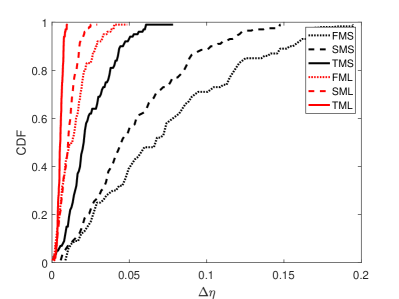
Figure 3: The CDFs of the absolute estimation error in the case of different order of the moments.

The result shown in Fig. 3 is obtained by numerically solving (30). The selected root of (30) satisfies $0<\eta<1$. The true value of $\eta$ is fixed at 0.5. Fig. 3 shows the CDFs of the absolute estimation error $\Delta\eta$ in the case of different order of the moments estimates. In the case of a small-size MU-MIMO system (with $M$=32, $N$ = $8$), FMS, SMS, and TMS are respectively referred to first-order, second-order, and third-order of moments estimates ($k=1\ or\ 2\ or\ 3$ in (30)). Similarly, FML, SML, and TML mean first-order, second-order, and third-order of moments estimates in a large-scale MU-MIMO system ($M$=256, $N$ = $30$), respectively. From Fig. 3, we can see that the estimation error decreases as the order of the moments increases. For the large-size MU-MIMO system, the maximum of absolute estimation error is less than 0.05, which is only $10\%$ of $\eta$, indicating the robustness of the proposed method. Besides, compared to the small-size MIMO system, better estimation performance can be obtained in MU-MIMO systems with large-size transmit antennas. However, it is noted that employing higher order of moments pays the price of higher computational complexity. In what follows, we respectively use first-order and third-order moments estimates to determine the unknown parameter $\eta$ in small-size ($M\leq 32$) and large-size ($M\geq 128$) systems.

IV-A2 The Effect of the System Size

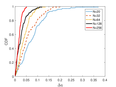
Figure 4: The CDFs of the absolute estimation error in the case of different number of transmit antennas.

We now investigate the effect of the system size on the estimation of $\eta$. We consider an $M$-antenna MU-MIMO system with QPSK signaling. Fig. 4 plots the CDFs of the absolute estimation error for different numbers of transmit antennas, whilst Fig. 5 shows the results for different numbers of UEs. In Fig. 4, the number of UEs is $N=20$. The numbers of antennas are 20, 32, 64, 128 and 256, respectively. It is shown in Fig. 4 that the estimation performance improves as the increase of the number of transmit antennas. In Fig. 5, the numbers of UEs are 5, 10, 15, 20, 20, and 30, respectively. The number of transmit antennas is $M=256$. The results in Fig. 5 imply that one can obtain accurate estimates of $\eta$ with high probability for various numbers of UEs. Besides, the estimation performance improves as the increase of the number of UEs. Interestingly, the estimation performance does not improve distinctly when the number of UEs is above a certain threshold (e.g., $N\geq 20$). We will revisit such a phenomenon with a theoretical analysis in our future work.

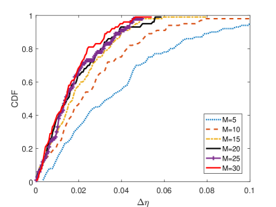
Figure 5: The CDFs of the absolute estimation error in the case of different number of UEs.

IV-B The Accuracy of Channel Matrix Reconstruction

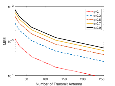
Figure 6: MSE of channel matrix reconstruction with different number of transmit antennas.

We consider the case with $N=20$ UEs and $M=20,32,64,128,256$ transmit antennas. In this case, the CSI is reconstructed by the proposed EI-based rotation invariant estimation method as shown in Algorithm 1. Let ${\bf{\hat{H}}}$ be the estimate of ${\bf{H}}$. Fig. 6 illustrates the the mean square error (MSE) of channel matrix reconstruction, which is denoted by

$${\rm{MSE=}}\frac{1}{{MN}}\left\|{{\bf{H}}-{\bf{\hat{H}}}}\right\|_{\mathop{\rm F}\nolimits}^{2}.$$

It is shown in Fig. 6 that the reconstruction error decreases as the increase in the number of transmit antennas. Besides, the proposed method can provide accurate estimates of CSI from noisy CSI in both small perturbation condition (e.g., $\eta=0.1$) and large perturbation condition (e.g., $\eta=0.9$), indicating the robustness of the new method.

IV-C BER Performance

In this experiment, we investigate the BER performance of coarsely quantized MU-MIMO systems with imperfect CSI in three cases. The BS is equipped with 256 transmit antennas and serves 30 UEs. For notation succinctness, we use EI to denote the proposed eigen-inference precoder. WF and WF0 are respectively referred to the WF precoding scheme implemented in the case of perfect CSI and imperfect CSI (without reconstruction). We have similar definition for other compared precoding schemes.

IV-C1 The Effect of Quantization Levels

Fig. 7 shows the BER of the WF variants versus signal-to-noise ratios (SNRs) for different quantization levels (B-bit DACs). The CSI-related parameter is fixed at $\eta=0.3$. From Fig. 7, we observe that the performance of the WF precoder (with perfect CSI) and the proposed WF-IE precoder (with imperfect CSI) improve with the increase of the quantization level. The results indicate that the proposed precoder can provide reliable transmission of QPSK signaling in the case of imperfect CSI. Specially, for $\{2,3,4\}$-bit quantization, the performance gap to ideal BER (perfect CSI) with that of WF-IE is only about 3 dB for a target BER of $10^{-3}$.

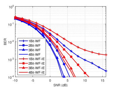
Figure 7: Performance of the proposed precoder with different quantization levels in the case of large MU-MIMO system with QPSK signaling.

IV-C2 The Effect of the SNR

In Fig. 8, we consider a massive MIMO system with 4-bit DACs. It is shown that the WF-IE percoder has similar performance with the ZF-IE precoder and outperforms the MRT-IE precoder. Moreover, the performance gap between the WF precoder with perfect CSI and the proposed WF-IE precoder (with imperfect CSI) is remarkably smaller than that between the WF precoder and the WF0 precoder. For example, for the same BER target of $10^{-3}$, the former is about 3 dB while the latter is more than 15 dB. The result implies that the implementation of robust precoding algorithms for coarsely quantized massive MIMO systems with imperfect CSI is helpful and possible by employing proper signal processing techniques (e.g., the proposed EI precoder).

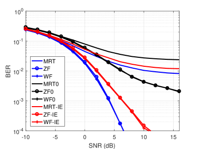
Figure 8: Uncoded BER of the compared precoders in the case of a quantized massive MU-MIMO system (128 BS antennas and 20 UTs) with QPSK signaling. The CSI-related parameter is fixed at $\eta=0.3$.

IV-C3 The Effect of Different Values of $\eta$

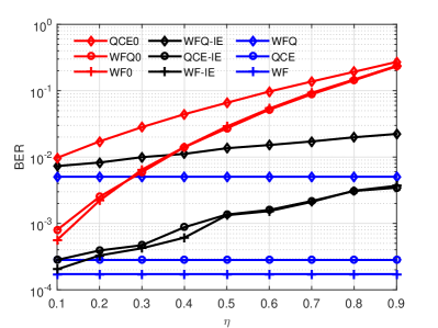
Figure 9: Uncoded BER of the compared precoders for the MU-MIMO system with 4-bit DACs and different values of $\eta$.

In Fig. 9, we show the BER performance of all the precoders with different values of $\eta$. The SNR is fixed at 5 dB, a low-to-moderate (typical) SNR. In the case of perfect CSI, the WF percoder outperforms the WFQ precoder, which is in line with the result in [23]. In the presence of imperfect CSI, it can be seen from Fig. 9 that each precoder degrades as the increase of $\eta$. However, they have different sensitivity, e.g., WFQ0, WF0 and QCE0 are more sensitive to errors in CSI than their counterparts using the proposed CSI reconstruction method. As a consequence, WFQ-IE, WF-IE and QCE-IE significantly outperform WFQ0, WF0 and QCE0, and the advantage increases as $\eta$ increases. For example, WFQ0 and WF0 can approach a target BER of $10^{-3}$ only when $\eta<0.15$, while WFQ-IE and WF-IE can achieve a target BER of $10^{-3}$ for any $\eta<0.45$. Even in the limit case of $\eta=0.9$, the proposed precoder can still achieve a BER of about $10^{-2.5}$. On the whole, the results imply that the employment of simplified hardware (low-resolution DACs) could be possible without severe BER performance loss in the case of imperfect CSI.

V Conclusions

In the paper, we developed a novel precoding scheme for coarsely quantized massive MU-MIMO systems in the presence of imperfect CSI. Firstly, we provided some analysis using the block random matrix theory, based on which the limiting spectra distribution connection between the true BSCA and noisy BSCA has been established. Then, with the obtained theoretical results, we proposed an EI-based moments matching method to estimate the CSI-related noise level and a rotation invariant estimation method to reconstruct the CSI. Finally, experimental results have demonstrated that, the proposed EI precoding scheme can significantly mitigate the deterioration caused by imperfect CSI in coarsely quantized massive MU-MIMO systems.

VI Acknowledgements

The authors would like to thank the AE and anonymous reviewers for their valuable suggestions and criticism which improve the quality of this work.

Appendix A Proof of Lemma III.1

$Proof:$ Following [46], one can expand the $Stieltjes$ transform of a random matrix $\bf{A}$ as

$${{\mathfrak{g}}_{\bf{A}}}\left(z\right)=-\frac{1}{z}\sum\limits_{k=0}^{\infty}{\frac{{\mathbb{E}\left[{{{\bf{A}}^{k}}}\right]}}{{{z^{k}}}}}.$$ (46)

If $\bf{{A}}$ is a square random matrix, i.e., ${\bf{A}}\in{\mathbb{C}}^{N\times N}$, then one can have, in large dimensional regime ,

$${\mathbb{E}\left[{{{\bf{A}}^{k}}}\right]}\equiv\mathbb{E}\left[{\frac{1}{N}{\rm tr}\left\{{{{\bf{A}}^{k}}}\right\}}\right].$$ (47)

The $Stieltjes$ transform of $\bf{D}$ can be written as

$$\begin{array}[]{c}{{\mathfrak{g}}_{\bf{D}}}\left(z\right)=-\frac{1}{z}\sum\limits_{k=0}^{\infty}{\frac{\mathbb{E}{\left[{{{\bf{D}}^{k}}}\right]}}{{{z^{k}}}}}\equiv\frac{1}{{M+N}}\mathbb{E}\left[{{\mathop{\rm tr}\nolimits}\left\{{{{\left({z{\bf{I}}-{\bf{D}}}\right)}^{-1}}}\right\}}\right].\end{array}$$ (48)

From the definition of $\bf D$ in (16):

$${\bf{D}}={\bf{B}}{{\bf{B}}^{\rm H}}=\left[{\begin{array}[]{*{20}{c}}{{\bf{H}}{{\bf{H}}^{\rm H}}}&0\\ 0&{{{\bf{H}}^{\rm H}}{\bf{H}}}\end{array}}\right],$$

one can have, using the inverse of the block matrix,

$${{\mathfrak{g}}_{\bf{D}}}\left(z\right) =\frac{1}{{M+N}}{\mathop{\rm tr}\nolimits}\left[{\begin{array}[]{*{20}{c}}{{{\left({z{\bf{I}}-{\bf{H}}{{\bf{H}}^{\rm H}}}\right)}^{-1}}}&0\\ 0&{{{\left({z{\bf{I}}-{{\bf{H}}^{\rm H}}{\bf{H}}}\right)}^{-1}}}\end{array}}\right]$$ (50)

$$=\frac{1}{{M+N}}\left[{{\mathop{\rm tr}\nolimits}{{\left({z{\bf{I}}-{\bf{H}}{{\bf{H}}^{\rm H}}}\right)}^{-1}}+{\mathop{\rm tr}\nolimits}{{\left({z{\bf{I}}-{{\bf{H}}^{\rm H}}{\bf{H}}}\right)}^{-1}}}\right]$$

$$=\frac{M}{{M+N}}{{\mathfrak{g}}_{{\bf{H}}{{\bf{H}}^{\rm H}}}}\left(z\right)+\frac{N}{{M+N}}{{\mathfrak{g}}_{{{\bf{H}}^{\rm H}}{\bf{H}}}}\left(z\right).$$ (A.4)

From Lemma 3.1 in [49], we have

$${{\mathfrak{g}}_{{{\bf{H}}^{\rm H}}{\bf{H}}}}\left(z\right)={\frac{M}{N}{{\mathfrak{g}}_{{\bf{H}}{{\bf{H}}^{\rm H}}}}\left(z\right)+\frac{{M-N}}{N}\frac{1}{z}}.$$ (51)

Let $q=M/N$, plugging (A.5) into (50) gives

$${{\mathfrak{g}}_{\bf{D}}}\left(z\right)=\frac{{2q}}{{q+1}}{{\mathfrak{g}}_{{\bf{H}}{{\bf{H}}^{\rm H}}}}\left(z\right)+\frac{{q-1}}{{q+1}}\frac{1}{z},$$ (52)

which is the result shown in Lemma III.1.

Appendix B Proof of Lemma III.2

From (16), we have ${\bf{D}}={\bf{B}}^{2}$. Let ${F_{\bf{B}}}\left(x\right)$ and ${F_{\bf{D}}}\left(x\right)$ be the empirical eigenvalue distribution of ${\bf{B}}$ and ${\bf{D}}$, respectively. Since the eigenvalues of ${\bf{B}}$ are the radicals of the eigenvalues of ${\bf{D}}$, let $\left[{\left({-\sqrt{b},-\sqrt{a}}\right)\cup\left({\sqrt{a},\sqrt{b}}\right)}\right]$ be the support of the eigenvalues of ${\bf{B}}$ and recall the definition of the $Stieltjes$ transform in (9), then we have

$${{\mathfrak{g}}_{\bf{B}}}\left(z\right) =\int_{\sqrt{a}}^{\sqrt{b}}{\frac{1}{{z-x}}{\mathop{\rm d}\nolimits}{F_{\bf{B}}}\left(x\right)+\int_{-\sqrt{b}}^{-\sqrt{a}}{\frac{1}{{z-x}}{\mathop{\rm d}\nolimits}{F_{\bf{B}}}\left(x\right)}}$$

$$=\int_{\sqrt{a}}^{\sqrt{b}}{\frac{1}{{z-x}}{\mathop{\rm d}\nolimits}{F_{\bf{B}}}\left(x\right)+\int_{\sqrt{a}}^{\sqrt{b}}{\frac{1}{{z+x}}{\mathop{\rm d}\nolimits}{F_{\bf{B}}}\left(x\right)}}$$

$$=\int_{\sqrt{a}}^{\sqrt{b}}{\frac{{2z}}{{{z^{2}}-{x^{2}}}}{\mathop{\rm d}\nolimits}{F_{\bf{B}}}\left(x\right)}$$

$$=\int_{a}^{b}{\frac{z}{{{z^{2}}-y}}{\mathop{\rm d}\nolimits}{F_{{{\bf{B}}^{2}}}}\left(y\right)}$$

$$=z{{\mathfrak{g}}_{\bf{D}}}\left({{z^{2}}}\right),$$ (B.1)

which completes the proof of Lemma III.2.

Appendix C Proof of Lemma III.3

We start with the definition of the $\mathcal{M}$ transform [46] of a random matrix $\bf A$, which is denoted by

$${\mathcal{M}_{\bf{A}}}\left(z\right)=\sum\limits_{k=1}^{\infty}{\mathbb{E}\left[{{{\bf{A}}^{k}}}\right]{z^{k}}},$$ (53)

or

$${\mathcal{M}_{\bf{A}}}\left(z\right)={z^{-1}}{{\mathfrak{g}}_{\bf{A}}}\left({{z^{-1}}}\right)+1.$$ (54)

Besides, the $S$ transform can be expressed with the $\mathcal{M}$ transform as

$${S_{\bf{A}}}\left(z\right)=\frac{{1+z}}{z}{\mathcal{M}}_{\bf{A}}^{-1}\left(z\right).$$ (55)

From (21) (or (B.1)), it follows that

$${{\mathcal{M}}_{\bf{B}}}\left(z\right)={z^{-1}}{{\mathfrak{g}}_{\bf{B}}}\left({{z^{-1}}}\right)+1={z^{-2}}{{\mathfrak{g}}_{\bf{D}}}\left({{z^{-2}}}\right)+1={{\mathcal{M}}_{\bf{D}}}\left({{z^{2}}}\right).$$ (56)

Substituting (C.4) into (C.3) yields

$${S_{\bf{B}}}\left(z\right) =\frac{{1+z}}{z}{\mathcal{M}}_{\bf{B}}^{-1}\left(z\right)$$

$$=\frac{{1+z}}{z}{\left[{{\mathcal{M}}_{\bf{D}}^{-1}\left(z\right)}\right]^{1/2}}$$

$$=\frac{{1+z}}{z}{\left[{\frac{z}{{1+z}}{S_{\bf{D}}}\left(z\right)}\right]^{1/2}},$$

or equivalently,

$${\left[{{S_{\bf{B}}}\left(z\right)}\right]^{2}}=\frac{{1+z}}{z}{S_{\bf{D}}}\left(z\right),$$ (57)

which completes the proof of Lemma III.3.

Appendix D Proof of Theorem III.1

With the technical results in Lemma III.1, Lemma III.2 and Lemma III.3, one can easily obtain Theorem III.1 by means of the transforms of random matrices.

From [46], the $Stieltjes$ transform of ${{\bf{H}}{{\bf{H}}^{\rm H}}}$ is

$${\mathfrak{g}_{{\bf{H}}{{\bf{H}}^{\rm H}}}}\left(z\right)=\frac{{1-q-z-\sqrt{{z^{2}}-2\left({q+1}\right)z+{{\left({q-1}\right)}^{2}}}}}{{2qz}}.$$ (58)

Plugging (D.1) into (20) (or (A.6)), we have

$${{\mathfrak{g}}_{\bf{D}}}\left(z\right) =\frac{{2q}}{{q+1}}{{\mathfrak{g}}_{{\bf{H}}{{\bf{H}}^{\rm H}}}}\left(z\right)+\frac{{q-1}}{{q+1}}\frac{1}{z}$$

$$=\frac{{-z-\sqrt{{z^{2}}-2\left({q+1}\right)z+{{\left({q-1}\right)}^{2}}}}}{{\left({q+1}\right)z}}.$$ (D.2)

With Lemma III.2, one can obtain the $Stieltjes$ transform of $\bf{B}$, which is denoted by

$${{\mathfrak{g}}_{\bf{B}}}\left(z\right)=\frac{{-z^{2}-\sqrt{{z^{4}}-2\left({q+1}\right)z^{2}+{{\left({q-1}\right)}^{2}}}}}{{\left({q+1}\right)z}}.$$ (59)

Given ${{\mathfrak{g}}_{\bf{B}}}\left(z\right)$, the inversion formula [46, 49] that yields the limiting probability density function of the eigenvalues of ${\bf{B}}$ is

$${{\mathfrak{g}}_{\bf{B}}}\left(z\right) =\mathop{\lim}\limits_{y\to{0^{+}}}\frac{1}{\pi}{\mathop{\Im}\nolimits}\left[{{g_{\bf{B}}}\left({x+{\mathop{\rm i}\nolimits}y}\right)}\right]$$

$$=\frac{{\sqrt{\left({{b^{2}}-{x^{2}}}\right)\left({{x^{2}}-{a^{2}}}\right)}}}{{\left({q+1}\right)\pi\left|x\right|}}+\frac{{1-q}}{{1+q}}\delta\left(x\right).$$ (D.4)

where $a\leq\left|x\right|\leq b$ and $a=1-\sqrt{q},b=1+\sqrt{q}.$ This completes the proof of Theorem III.1.

Appendix E Proof of Theorem III.2

For the BSCA ${\bf{\widetilde{B}}}$, from (D.3), we have

$${{\mathfrak{g}}_{\bf{B}}}\left(z\right) =\frac{{-z^{2}-\sqrt{{z^{4}}-2\left({q+1}\right)z^{2}+{{\left({q-1}\right)}^{2}}}}}{{\left({q+1}\right)z}},$$

$$=\frac{{2q}}{{q+1}}{{\mathfrak{g}}_{\bf{\mathord{\buildrel{\lower 3.0pt\hbox{$\scriptscriptstyle\smile$}}\over{B}}}}}\left(z\right)+\frac{{q-1}}{{2qz}},$$ (E.1)

where ${\bf{\mathord{\buildrel{\lower 3.0pt\hbox{$\scriptscriptstyle\smile$}}\over{B}}}}$ is an auxiliary matrix whose $Stieltjes$ transform satisfies (E.1). With Lemma III.1, Lemma III.2, we can have

$${{\mathfrak{g}}_{\bf{\mathord{\buildrel{\lower 3.0pt\hbox{$\scriptscriptstyle\smile$}}\over{B}}}}}\left(z\right)=z{{\mathfrak{g}}_{{\bf H}{{\bf H}^{\rm H}}}}\left({{z^{2}}}\right).$$ (60)

Using (E.2) and Lemma III.3, one can obtain the $S$ transform of ${\bf{\mathord{\buildrel{\lower 3.0pt\hbox{$\scriptscriptstyle\smile$}}\over{B}}}}$, which can be denoted by

$${\left[{{S_{\bf{\mathord{\buildrel{\lower 3.0pt\hbox{$\scriptscriptstyle\smile$}}\over{B}}}}}\left(z\right)}\right]^{2}}=\frac{{1+z}}{z}{S_{{\bf H}{{\bf H}^{\rm H}}}}\left(z\right).$$ (61)

The relation between the $R$ transform and the $S$ transform has to satisfy [49, 58]

$$\frac{1}{{R\left(z\right)}}=S\left(z{R\left(z\right)}\right).$$ (62)

Plugging (E.3) into (E.4) gives

$${\left[{\frac{1}{{{R_{{\bf{\mathord{\buildrel{\lower 3.0pt\hbox{$\scriptscriptstyle\smile$}}\over{B}}}}}}\left(z\right)}}}\right]^{2}}={\left[{{S_{{\bf{\mathord{\buildrel{\lower 3.0pt\hbox{$\scriptscriptstyle\smile$}}\over{B}}}}}}\left({z{R_{{\bf{\mathord{\buildrel{\lower 3.0pt\hbox{$\scriptscriptstyle\smile$}}\over{B}}}}}}\left(z\right)}\right)}\right]^{2}}=\frac{{z+1}}{z}{S_{{\bf{H}}{{\bf{H}}^{\rm H}}}}\left({z{R_{{\bf{\mathord{\buildrel{\lower 3.0pt\hbox{$\scriptscriptstyle\smile$}}\over{B}}}}}}\left(z\right)}\right)$$ (63)

Since ${S_{{\bf{H}}{{\bf{H}}^{\rm H}}}}\left(z\right)=\frac{1}{{1+qz}}$ [49, 46], one can obtain the $R$ transform of ${\bf{\mathord{\buildrel{\lower 3.0pt\hbox{$\scriptscriptstyle\smile$}}\over{B}}}}$ by solving the equation (E.5), which yields

$${R_{{\bf{\mathord{\buildrel{\lower 3.0pt\hbox{$\scriptscriptstyle\smile$}}\over{B}}}}}}\left(z\right)=\frac{{-1+q{z^{2}}+\sqrt{1+4{z^{2}}-2q{z^{2}}+{q^{2}}{z^{4}}}}}{{2z}}.$$ (64)

For the noisy BSCA ${\bf{\widetilde{B}}}$, one can similarly define an auxiliary matrix ${\bf{\mathord{\buildrel{\lower 3.0pt\hbox{$\scriptscriptstyle\frown$}}\over{B}}}}$ that

$${{\mathfrak{g}}_{\bf{\mathord{\buildrel{\lower 3.0pt\hbox{$\scriptscriptstyle\frown$}}\over{B}}}}}\left(z\right)=z{{\mathfrak{g}}_{{\bf{\widetilde{H}}}{{\bf{\widetilde{H}}}^{\rm H}}}}\left({{z^{2}}}\right),$$ (65)

Combined with the addition law [46] shown in (23) and Lemma 4.1 in [49], the obtained $R$ transform of ${\bf{\mathord{\buildrel{\lower 3.0pt\hbox{$\scriptscriptstyle\frown$}}\over{B}}}}$ reads

$${R_{{\bf{\mathord{\buildrel{\lower 3.0pt\hbox{$\scriptscriptstyle\frown$}}\over{B}}}}}}\left(z\right)=\frac{{-1+q{z^{2}}+h\left(z\right)}}{{2z}},$$ (66)

where

$$h\left(z\right) =\sqrt{1+z^{2}\left({4+q\left({-2+qz^{2}}\right)}\right)}$$

$$+\sqrt{1+{\alpha^{2}}z^{2}\left({4+q\left({-2+z^{2}{\alpha^{2}}q}\right)}\right)}.$$

From (10), we can have

$${R_{{\bf{\mathord{\buildrel{\lower 3.0pt\hbox{$\scriptscriptstyle\frown$}}\over{B}}}}}}\left({\mathfrak{g}_{{\bf{\mathord{\buildrel{\lower 3.0pt\hbox{$\scriptscriptstyle\frown$}}\over{B}}}}}}\left(z\right)\right)=z-\frac{1}{{\mathfrak{g}_{{\bf{\mathord{\buildrel{\lower 3.0pt\hbox{$\scriptscriptstyle\frown$}}\over{B}}}}}}\left(z\right)}.$$ (67)

Finally, plugging (E.7) and (E.8) into (E.9) and solving (E.9) yields the technical result shown in Theorem III.2, which completes the proof.

References

- [1] L. Lu, G. Y. Li, A. L. Swindlehurst, A. Ashikhmin, and R. Zhang, “An overview of massive mimo: Benefits and challenges,” IEEE Journal of Selected Topics in Signal Processing, vol. 8, no. 5, pp. 742–758, 2014.
- [2] E. G. Larsson, O. Edfors, F. Tufvesson, and T. L. Marzetta, “Massive mimo for next generation wireless systems,” IEEE Communications Magazine, vol. 52, no. 2, pp. 186–195, 2014.
- [3] F. Rusek, D. Persson, B. K. Lau, E. G. Larsson, T. L. Marzetta, O. Edfors, and F. Tufvesson, “Scaling up mimo: Opportunities and challenges with very large arrays,” Signal Processing Magazine IEEE, vol. 30, no. 1, pp. 40–60, 2012.
- [4] M. Joham, W. Utschick, and J. A. Nossek, “Linear transmit processing in mimo communications systems,” IEEE Transactions on Signal Processing, vol. 53, no. 8, pp. 2700–2712, 2005.
- [5] N. Jindal and A. Goldsmith, “Dirty paper coding vs. tdma for mimo broadcast channels,” IEEE Transactions on Information Theory, vol. 51, no. 5, pp. 1783–1794, 2005.
- [6] J. Zhang, L. Dai, L. Xu, L. Ying, and L. Hanzo, “On low-resolution adcs in practical 5g millimeter-wave massive mimo systems,” IEEE Communications Magazine, vol. PP, no. 99, pp. 2–8, 2018.
- [7] A. H. Gokceoglu, E. Bjornson, E. G. Larsson, and M. Valkama, “Spatio-temporal waveform design for multiuser massive mimo downlink with 1-bit receivers,” IEEE Journal of Selected Topics in Signal Processing, vol. 11, no. 2, pp. 347–362, 2017.
- [8] J. Guerreiro, R. Dinis, and P. Montezuma, “Use of 1-bit digital-to-analogue converters in massive mimo systems,” Electronics Letters, vol. 52, no. 9, pp. 778–779, 2016.
- [9] Z. Zhang, C. Xiao, C. Li, C. Zhong, and H. Dai, “One-bit quantized massive mimo detection based on variational approximate message passing,” IEEE Transactions on Signal Processing, vol. PP, no. 99, pp. 1–1, 2017.
- [10] P. Dong, Z. Hua, X. Wei, and X. You, “Efficient low-resolution adc relaying for multiuser massive mimo system,” IEEE Transactions on Vehicular Technology, vol. PP, no. 99, pp. 1–1, 2017.
- [11] O. B. Usman, J. A. Nossek, C. A. Hofmann, and A. Knopp, “Joint mmse precoder and equalizer for massive mimo using 1-bit quantization,” in IEEE International Conference on Communications, 2017.
- [12] H. H. Yang, G. Geraci, T. Q. S. Quek, and J. G. Andrews, “Cell-edge-aware precoding for downlink massive mimo cellular networks,” IEEE Transactions on Signal Processing, vol. PP, no. 99, pp. 1–1, 2017.
- [13] A. K. Saxena, I. Fijalkow, and A. L. Swindlehurst, “On one-bit quantized zf precoding for the multiuser massive mimo downlink,” in Conference on Signals, Systems & Computers, 2016.
- [14] J. Mo, A. Alkhateeb, S. Abu-Surra, and J. R. W. Heath, “Hybrid architectures with few-bit adc receivers: Achievable rates and energy-rate tradeoffs,” IEEE Transactions on Wireless Communications, vol. 16, no. 4, pp. 2274–2287, 2017.
- [15] C. Kong, A. Mezghani, C. Zhong, A. L. Swindlehurst, and Z. Zhang, “Multipair massive mimo relaying systems with one-bit adc s and dac s,” IEEE Transactions on Signal Processing, vol. 66, no. 11, pp. 2984–2997, 2018.
- [16] Y. Li, T. Cheng, A. L. Swindlehurst, A. Mezghani, and L. Liu, “Downlink achievable rate analysis in massive mimo systems with one-bit dacs,” IEEE Communications Letters, vol. 21, no. 7, pp. 1669–1672, 2017.
- [17] J. H and N. J, “On the statistical properties of constant envelope quantizers,” IEEE Wireless Communications Letters, vol. PP, no. 99, pp. 1–1, 2018.
- [18] S. Jacobsson, G. Durisi, M. Coldrey, and C. Studer, “Massive mu-mimo-ofdm downlink with one-bit dacs and linear precoding,” global communications conference, pp. 1–6, 2017.
- [19] C. Studer and G. Durisi, “Quantized massive mu-mimo-ofdm uplink,” IEEE Transactions on Communications, vol. 64, no. 6, pp. 2387–2399, 2016.
- [20] C. Mollen, J. Choi, E. G. Larsson, and R. W. Heath, “Uplink performance of wideband massive mimo with one-bit adcs,” IEEE Transactions on Wireless Communications, vol. 16, no. 1, pp. 87–100, 2017.
- [21] C. K. Wen, C. J. Wang, J. Shi, K. K. Wong, and P. Ting, “Bayes-optimal joint channel-and-data estimation for massive mimo with low-precision adcs,” IEEE Transactions on Signal Processing, vol. 64, no. 10, pp. 2541–2556, 2016.
- [22] S. Jacobsson, G. Durisi, M. Coldrey, T. Goldstein, and C. Studer, “Nonlinear 1-bit precoding for massive mu-mimo with higher-order modulation,” asilomar conference on signals, systems and computers, pp. 763–767, 2016.
- [23] ——, “Quantized precoding for massive mu-mimo,” IEEE Transactions on Communications, vol. 65, no. 11, pp. 4670–4684, 2017.
- [24] H. Jedda, J. A. Nossek, and A. Mezghani, “Minimum ber precoding in 1-bit massive mimo systems,” in Sensor Array & Multichannel Signal Processing Workshop, 2016.
- [25] O. Castaneda, S. Jacobsson, G. Durisi, M. Coldrey, T. Goldstein, and C. Studer, “1-bit massive mu-mimo precoding in vlsi,” IEEE Journal on Emerging and Selected Topics in Circuits and Systems, vol. 7, no. 4, pp. 508–522, 2017.
- [26] C. Wang, C. Wen, S. Jin, and S. Tsai, “Finite-alphabet precoding for massive mu-mimo with low-resolution dacs,” IEEE Transactions on Wireless Communications, vol. 17, no. 7, pp. 4706–4720, 2018.
- [27] L. Chu, W. Fei, L. Lily, and Q. Robert, “Efficient nonlinear precoding for massive mu-mimo downlink systems with 1-bit dacs,” Revised for IEEE Transactions on Wireless Communications, 2018. [Online]. Available: https://arxiv.org/abs/1804.08839
- [28] I. C. Wong and B. L. Evans, “Optimal resource allocation in the ofdma downlink with imperfect channel knowledge,” IEEE Transactions on Communications, vol. 57, no. 1, pp. 232–241, 2009.
- [29] M. Ding and S. D. Blostein, “Maximum mutual information design for mimo systems with imperfect channel knowledge,” IEEE Transactions on Information Theory, vol. 56, no. 10, pp. 4793–4801, 2010.
- [30] A. Mukherjee and A. L. Swindlehurst, “Robust beamforming for security in mimo wiretap channels with imperfect csi,” IEEE Transactions on Signal Processing, vol. 59, no. 1, pp. 351–361, 2010.
- [31] M. Rezk and B. Friedlander, “On high performance mimo communications with imperfect channel knowledge,” IEEE Transactions on Wireless Communications, vol. 10, no. 2, pp. 602–613, 2011.
- [32] N. Lee, O. Simeone, and J. Kang, “The effect of imperfect channel knowledge on a mimo system with interference,” IEEE Transactions on Communications, vol. 60, no. 8, pp. 2221–2229, 2012.
- [33] M. H. Al-Ali and K. C. Ho, “Transmit precoding in underlay mimo cognitive radio with unavailable or imperfect knowledge of primary interference channel,” IEEE Transactions on Wireless Communications, vol. 15, no. 8, pp. 5143–5155, 2016.
- [34] N. I. Miridakis and T. A. Tsiftsis, “On the joint impact of hardware impairments and imperfect csi on successive decoding,” IEEE Transactions on Vehicular Technology, vol. 66, no. 6, pp. 4810–4822, 2017.
- [35] B. J, “Crosscorrelation functions of amplitude-distorted gaussian signals,” Bell Lab Technical Report, vol. Rept. 216, 1952.
- [36] R. R. Far, T. Oraby, W. Bryc, and R. Speicher, “On slow-fading mimo systems with nonseparable correlation,” IEEE Transactions on Information Theory, vol. 54, no. 2, pp. 544–553, 2008.
- [37] T. Oraby, “The limiting spectra of girko s block-matrix,” Journal of Theoretical Probability, vol. 20, no. 4, pp. 959–970, 2007.
- [38] H. Dette and B. Reuther, “Random block matrices and matrix orthogonal polynomials,” Journal of Theoretical Probability, vol. 23, no. 2, pp. 378–400, 2010.
- [39] G. Caire, N. Jindal, M. Kobayashi, and N. Ravindran, “Multiuser mimo achievable rates with downlink training and channel state feedback,” IEEE Transactions on Information Theory, vol. 56, no. 6, pp. 2845–2866, 2007.
- [40] ——, “Quantized vs. analog feedback for the mimo broadcast channel: A comparison between zero-forcing based achievable rates,” in IEEE International Symposium on Information Theory, 2007.
- [41] J. Guerreiro, D. Rui, and P. Montezuma, “Analytical performance evaluation of precoding techniques for nonlinear massive mimo systems with channel estimation errors,” IEEE Transactions on Communications, vol. 66, no. 4, pp. 1440–1451, 2018.
- [42] N. K. Le, “Secrecy and end-to-end analyses employing opportunistic relays under outdated channel state information and dual correlated rayleigh fading,” IEEE Transactions on Vehicular Technology, vol. 67, no. 11, pp. 10 504–10 518, 2018.
- [43] A. Mezghani, R. Ghiat, and J. A. Nossek, “Transmit processing with low resolution d/a-converters,” in IEEE International Conference on Electronics, 2009.
- [44] J. Bun, J. P. Bouchaud, and M. Potters, “Cleaning large correlation matrices: Tools from random matrix theory,” Physics Reports, vol. 666, p. S0370157316303337, 2016.
- [45] J. Bun, R. Allez, J. P. Bouchaud, and M. Potters, “Rotational invariant estimator for general noisy matrices,” IEEE Transactions on Information Theory, vol. PP, no. 99, pp. 1–1, 2015.
- [46] A. M. Tulino and S. Verdú, “Random matrix theory and wireless communications,” Commun. Inf. Theory, vol. 1, no. 1, pp. 1–182, Jun. 2004. [Online]. Available: http://dx.doi.org/10.1516/0100000001
- [47] V. L. Girko, “Circular law,” Theory of Probability and Its Applications, vol. 29, no. 4, pp. 694–706, 1984.
- [48] T. Terence, Topics in Random Matrix Theory. American Mathematical Society, 2012.
- [49] R. Couillet and M. Debbah, Random Matrix Methods for Wireless Communications. U.K.:Cambridge Univ. Press, 2012.
- [50] T. A., “An orthogonally invariant minimax estimator of the covariance matrix of a multivariate normal population,” Tsukuba journal of mathematics, vol. 8, no. 2, pp. 367–376, 1984.
- [51] S. Kay, “Fundamentals of statistical signal processing: estimation theory,” Technometrics, vol. 37, no. 4, p. 465, 1993.
- [52] G. Schwarz, “Estimating the dimension of a model,” Annals of Statistics, vol. 6, no. 2, pp. 461–464, 1978.
- [53] D. Jimenez, L. Wang, and Y. Wang, “White noise hypothesis for uniform quantization errors.” Siam Journal on Mathematical Analysis, vol. 38, no. 6, pp. 2042–2056, 2015.
- [54] A. K. Saxena, I. Fijalkow, and A. L. Swindlehurst, “Analysis of one-bit quantized precoding for the multiuser massive mimo downlink,” IEEE Transactions on Signal Processing, vol. 65, no. 17, pp. 4624–4634, 2017.
- [55] A. J. Stothers, “On the complexity of matrix multiplication,” Ph.D. dissertation, University of Edinburgh, 2010.
- [56] P. Kun II, Fundamentals of Probability and Stochastic Processes with Applications to Communications. Springer International Publishing, 2018.
- [57] R. Couillet, F. Pascal, and J. W. Silverstein, “Robust estimates of covariance matrices in the large dimensional regime,” Information Theory IEEE Transactions on, vol. 60, no. 11, pp. 7269–7278, 2012.
- [58] R. C. Qiu and P. Antonik, Smart Grid and Big Data: Theory and Practice. Wiley Publishing, 2017.