Magnetic moments of the spin-$1\over 2$ singly charmed baryons in chiral perturbation theory

Abstract

We systematically derive the analytical expressions of the magnetic moments of the spin-$1\over 2$ singly charmed baryons to the next-to-next-to-leading order in the heavy baryon chiral perturbation theory (HBChPT). We discuss the analytical relations between the magnetic moments. We estimate the-low energy constants (LECs) in two scenarios. In the first scenario, we use the quark model and Lattice QCD simulation results as input. In the second scenario, the heavy quark symmetry is adopted to reduce the number of the independent LECs, which are then fitted using the data from the Lattice QCD simulations. We give the numerical results to the next-to-leading order for the antitriplet charmed baryons and to the next-to-next-to-leading order for the sextet states.

I Introduction

In the past decades, many heavy baryons and their excitations have been observed in experiments [1]. For instance, the $\Omega_{c}^{*}$ was observed in the decay channel $\Omega_{c}^{*}\rightarrow\Omega_{c}\gamma$ by the BABAR Collaboration and confirmed by the Belle Collaboration [2, 3]. The other two radiative decay processes, $\Xi_{c}^{{}^{\prime}+}\rightarrow\Xi_{c}^{+}\gamma$ and $\Xi_{c}^{{}^{\prime}0}\rightarrow\Xi_{c}^{0}\gamma$ were also observed in experiments [4, 5, 6]. The electromagnetic processes become more important when strong decay processes are forbidden due to the phase space. These processes provide a platform to study their electromagnetic properties, which are very important to explore the inner structures of the heavy baryons. More experiment data about the magnetic moment and other electromagnetic properties from PANDA, LHCb, BESIII, Belle II and so on are expected in the future.

The electromagnetic properties of the heavy baryons have attracted the attention of many theorists. Many theoretical models have been adopted to study the electromagnetic properties of the heavy baryons. The radiative decays of the heavy baryons were investigated with the chiral symmetry and heavy quark symmetry in Ref. [7]. In Ref. [8], the radiative decay $\Sigma^{*0}_{c}\rightarrow\Lambda_{c}^{0}+\gamma$ was studied in chiral perturbation theory. In Refs. [9, 10, 11], the electromagnetic decays of the heavy baryons have been calculated in the framework of the heavy baryon chiral perturbation theory. In Refs. [12, 13, 14, 15], the authors studied the radiative decay and magnetic moments of the heavy baryons with the Lattice QCD simulation. The radiative decays and magnetic moments of the heavy baryons were also studied using the heavy quark symmetry [16], various quark models [17, 18, 19, 20, 21, 22, 23, 24], QCD sum rule formalism [25, 26] and the bag model [27]. In addition, the magnetic moments of the heavy baryons have been calculated in the bag model [28, 29, 30], the QCD sum rules [31, 32, 33], the effective quark mass and screened charge scheme [34], the hyper central model [35], the quark-diquark Model [36], the skyrme model [37, 38], the mean-field approach [39], the bound-state approach [40], and the heavy hadron chiral perturbation theory [11, 41, 42]. In Ref. [43], the magnetic moments and charge radii of the $\Sigma_{c}$ and $\Omega_{c}$ were calculated with the Lattice QCD simulations.

The chiral perturbation theory (ChPT) is a very useful tool to study the hadron properties at the low-energy regime. However, the heavy baryon mass introduces a new large scale and does not vanish in the chiral limit, which destroys the chiral power counting. Three methods were proposed to overcome this obstacle, the heavy baryon chiral perturbation theory (HBChPT) [44, 45, 46], the infrared regularization (IR) [47], and the extended-on-mass-shell regularization (EOMS) [48, 49]. The IR and the EOMS are the relativistic formalization of the chiral perturbation theory. They have been used to study the electromagnetic properties of baryons [50, 51, 52]. In the HBChPT, the heavy baryon field is decomposed into the “light” and “heavy” components. The “heavy” component is integrated out. Then, the expansion is in powers of the momentum (mass) of the pseudoscalar meson and the residue momentum of the heavy baryon. The chiral power counting is recovered. The HBChPT formalism has been used to study the electromagnetic properties of the octet and decuplet baryons [53, 54, 55, 56]. The masses of the charmed baryons are large, which are about $2.5$ GeV. In this case, the recoil effect is negligible. The heavy baryon chiral perturbation theory is suitable in calculating the magnetic moments of the heavy baryons.

In Refs. [11, 42], the authors have calculated the magnetic moments of the heavy baryons up to next-to-leading order (NLO) using the (partially quenched) heavy hadron chiral perturbation theory. The wave-function renormalization, the vertex renormalization, and other effects are not included up to this order. However, they may not be negligible. For instance, the wave-function renormalization contributes a nonanalytic $m_{q}\text{ln}m_{q}$ ($m_{q}$ is the light quark mass.) correction to the magnetic moments of the baryons [56, 55]. To include the above effects, we have considered all the one-loop diagrams. And we calculate the analytical expressions of the magnetic moments up to the next-to-next-to-leading order (NNLO). Several relations of magnetic moments were given up to NLO in Ref. [42]. We find most of these relations are not valid any more at NNLO.

The paper is arranged as follows. In Sec. II, we give the effective Lagrangians that contribute to the magnetic moments. In Sec. III, we calculate the analytical expressions of the magnetic moments of the antitriplet and the sextet charmed baryons. In Sec. IV, we obtain the numerical results. The magnetic moments of antri-triplet charmed baryons are given to $\mathcal{O}(p^{2})$. The numerical results of sextet charmed baryons are given up to $\mathcal{O}(p^{3})$ in two scenarios. The last section is a brief summary. Finally, some calculation details and explicit loop integrals are collected in the Appendix.

II The Effective Lagrangians

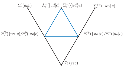
Figure 1: The blue and black triangles denote the heavy baryons in the $\bar{3}_{f}$ and the $6_{f}$ flavor representations, respectively. $[...]$ and $\{...\}$ denotes the two light quarks are antisymmetric and symmetric in the flavor space, respectively.

In the SU(3) flavor symmetry, the two light quarks in the heavy baryon form the antisymmetric $\bar{3}_{f}$ and the symmetric $6_{f}$ representations as illustrated in Fig. 1. The total spin of the light quarks is $S_{l}=0$ or $S_{l}=1$, respectively. The spin of the antitriplet heavy baryon is $S_{{\bar{3}}}=\frac{1}{2}$ and the spin of the sextet heavy baryon is $\frac{1}{2}$ or $\frac{3}{2}$. We denote the above three kinds of states as $\psi_{{\bar{3}}}$, $\psi_{6}$ and $\psi^{*\mu}_{6}$ respectively.

$$\quad\psi_{{\bar{3}}}=\left(\begin{array}[]{ccc}0&\Lambda_{c}^{+}&\Xi_{c}^{+}\\ -\Lambda_{c}^{+}&0&\Xi_{c}^{0}\\ -\Xi_{c}^{+}&-\Xi_{c}^{0}&0\end{array}\right),\quad\psi_{{6}}=\left(\begin{array}[]{ccc}\Sigma_{c}^{++}&\frac{\Sigma_{c}^{+}}{\sqrt{2}}&\frac{\Xi_{c}^{\prime+}}{\sqrt{2}}\\ \frac{\Sigma_{c}^{+}}{\sqrt{2}}&\Sigma_{c}^{0}&\frac{\Xi_{c}^{\prime 0}}{\sqrt{2}}\\ \frac{\Xi_{c}^{\prime+}}{\sqrt{2}}&\frac{\Xi_{c}^{\prime 0}}{\sqrt{2}}&\Omega_{c}^{0}\end{array}\right),\quad\psi_{6}^{*\mu}=\left(\begin{array}[]{ccc}\Sigma_{c}^{*++}&\frac{\Sigma_{c}^{*+}}{\sqrt{2}}&\frac{\Xi_{c}^{*+}}{\sqrt{2}}\\ \frac{\Sigma_{c}^{*+}}{\sqrt{2}}&\Sigma_{c}^{*0}&\frac{\Xi_{c}^{*0}}{\sqrt{2}}\\ \frac{\Xi_{c}^{*+}}{\sqrt{2}}&\frac{\Xi_{c}^{*0}}{\sqrt{2}}&\Omega_{c}^{*0}\end{array}\right)^{\mu}.$$ (10)

In the HBChPT scheme, we decompose the heavy baryon fields into the “heavy” and “light” components as follows

$$B_{n}(x)=e^{iM_{B}v\cdot x}\frac{1+\not{v}}{2}\psi_{n},~{}~{}H_{n}(x)=e^{iM_{B}v\cdot x}\frac{1-\not{v}}{2}\psi_{n},$$ (11)

where $\psi_{n}$ denotes the heavy baryon field $\psi_{{\bar{3}}}$, $\psi_{6}$ or $\psi^{*\mu}_{6}$, and $B_{n}$ ($H_{n}$) is the “light” (“heavy”) component of the corresponding heavy baryon field. $M_{B}$ is the baryon mass, and $v^{\mu}=(1,\vec{0})$ is the static velocity. The heavy field $H_{n}(x)$ is then integrated out in the Lagrangians.

In the HBChPT scheme, the matrix element of the electromagnetic current for the spin-$\frac{1}{2}$ heavy baryon is

$$\langle B_{\bar{3}}(p^{\prime})|\mathcal{J}_{\mu}|B_{\bar{3}}(p)\rangle=\bar{u}(p^{\prime})\left(v_{\mu}G_{E}(q^{2})+\frac{[S_{\mu},S\cdot q]}{M_{B}}G_{M}(q^{2})\right)u(p),$$ (12)

where $\mathcal{J}_{\mu}$ is the electromagnetic current, and $q=p^{\prime}-p$ is the transferred momentum. $u(p)$ and $\bar{u}(p)$ represent the Dirac spinors for the initial and finial heavy baryons with the momentum $p$, respectively. $S^{\mu}$ is the spin operator $\frac{i}{2}\gamma^{5}\sigma^{\mu\nu}v_{\nu}$. $G_{E}$ and $G_{M}$ are the electric and magnetic form factors, respectively. The magnetic moment $\mu_{B}=\frac{e}{2M_{B}}G_{M}(0)$.

II.1 The leading-order Lagrangians

The pseudoscalar mesons are denoted as

$$\phi=\sqrt{2}\left(\begin{array}[]{ccc}\frac{\pi^{0}}{\sqrt{2}}+\frac{\eta}{\sqrt{6}}&\pi^{+}&K^{+}\\ \pi^{-}&-\frac{\pi^{0}}{\sqrt{2}}+\frac{\eta}{\sqrt{6}}&K^{0}\\ K^{-}&\overline{K}^{0}&-\frac{2}{\sqrt{6}}\eta\end{array}\right).$$ (16)

The Lagrangian for the pseudoscalar mesons at the leading order is

$$\mathcal{L}^{(2)}=\frac{F^{2}_{0}}{4}\text{Tr}[\triangledown_{\mu}U{\triangledown^{\mu}U}^{\dagger}],$$ (17)

with

$$U=\xi^{2}=e^{\frac{i\phi}{F_{0}}},\quad \triangledown_{\mu}U=\partial_{\mu}U+ieA_{\mu}[Q_{l},U],$$ (18)

where $F_{0}$ is the decay constant in the chiral limit. In this work, we use the values $F_{\pi}=92.4$ MeV, $F_{K}=113$ MeV, and $F_{\eta}=116$ MeV after renormalization, respectively. $A_{\mu}$ is the electromagnetic field. The charge matrix for the light quark is $Q_{l}=\text{diag}(2/3,-1/3,-1/3)$.

The leading-order Lagrangians related to the heavy baryons are

$$\mathcal{L}_{0}^{(1)} = \frac{1}{2}\text{Tr}[{\bar{\psi}}_{{\bar{3}}}(i\not{D}-M_{{\bar{3}}})\psi_{{\bar{3}}}]+\text{Tr}[{\bar{\psi}}_{6}(i\not{D}-M_{6})\psi_{6}]$$ (19)

$$+\text{Tr}\left[{\bar{\psi}}_{6}^{*\mu}(-g_{\mu\nu}(i\not{D}-M_{6^{*}})+i(\gamma_{\mu}D_{\nu}+\gamma_{\nu}D_{\mu})-\gamma_{\mu}(i\not{D}+M_{6^{*}})\gamma_{\nu})\psi_{6}^{*\nu}\right]$$

$$\mathcal{L}_{\textrm{int}}^{(1)} = g_{1}\textrm{Tr}({\bar{\psi}}_{6}\not{u}\gamma_{5}\psi_{6})+g_{2}\textrm{Tr}[({\bar{\psi}}_{6}\not{u}\gamma_{5}\psi_{{\bar{3}}})+\textrm{H.c.}]+g_{3}\textrm{Tr}[({\bar{\psi}}_{6}^{*\mu}u_{\mu}\psi_{6})+\textrm{H.c.}]$$ (20)

$$+g_{4}\textrm{Tr}[({\bar{\psi}}_{6}^{*\mu}u_{\mu}\psi_{{\bar{3}}})+\textrm{H.c.}]+g_{5}\textrm{Tr}({\bar{\psi}}_{6}^{*\nu}\not{u}\gamma_{5}\psi_{6\nu}^{*})+g_{6}\textrm{Tr}({\bar{\psi}}_{{\bar{3}}}\not{u}\gamma_{5}\psi_{{\bar{3}}}).$$

with the covariant derivatives and $u_{\mu}$ defined as

$$D_{\mu}\psi_{B}=\partial_{\mu}\psi_{B}+\Gamma_{\mu}\psi_{B}+\psi_{B}\Gamma_{\mu}^{T},$$

$$\Gamma_{\mu}=\frac{1}{2}(\xi^{\dagger}\partial_{\mu}\xi+\xi\partial_{\mu}\xi^{\dagger})+\frac{i}{2}eA_{\mu}(\xi^{\dagger}Q_{B}\xi+\xi Q_{B}\xi^{\dagger}),$$

$$u_{\mu}=\frac{i}{2}(\xi^{\dagger}\partial_{\mu}\xi-\xi\partial_{\mu}\xi^{\dagger})-\frac{1}{2}eA_{\mu}(\xi^{\dagger}Q_{B}\xi-\xi Q_{B}\xi^{\dagger}),$$

where the charge operator of the heavy baryon $Q_{B}=\text{diag}(1,0,0)$. In this work, the mass difference among the antitriplet multiplet and the sextet multiplet is neglected. We use the average masses $M_{{}_{\bar{3}}}=2408$ MeV, $M_{{}_{6}}=2535$ MeV, and $M_{6^{*}}=2602$ MeV, respectively [1].

$g_{i}$ is the coupling for the interaction between the pseudoscalar mesons and heavy baryons. $g_{2,4}$ are calculated through the widths of the heavy baryons. $g_{1,3,5}$ are related to $g_{2,4}$ with the help of the quark model. Their values are [57, 58, 9]

$$g_{1}=0.98,\quad g_{2}=-\sqrt{\frac{3}{8}}g_{1}=-0.60,\quad g_{3}=\frac{\sqrt{3}}{2}g_{1}=0.85,$$

$$g_{4}=-\sqrt{3}g_{2}=1.04,\quad g_{5}=-\frac{3}{2}g_{1}=-1.47,\quad g_{6}=0.$$ (21)

The pseudoscalar mesons only interact with the light quarks inside the heavy baryons, and the total spin of light quarks is $S_{l}=0$ for the baryon in the antitriplet. The $\phi B_{\bar{3}}B_{\bar{3}}$ vertex is therefore forbidden considering the parity and angular momentum conservation, and thus $g_{6}=0$.

The nonrelativistic Lagrangian at the leading order can be directly derived from the $\mathcal{L}_{0}^{(1)}+\mathcal{L}_{int}^{(1)}$ [57, 58],

$$\mathcal{L}_{MB}^{(1)} = \frac{1}{2}\text{Tr}(\bar{B}_{\bar{3}}iv\cdot DB_{\bar{3}})+\text{Tr}(\bar{B}_{6}(iv\cdot D-\delta_{1})B_{6})-\text{Tr}(\bar{B}_{6}^{*\mu}(iv\cdot D-\delta_{2})B_{6\mu}^{*})$$ (22)

$$+2g_{1}\text{Tr}(\bar{B}_{6}S\cdot uB_{6})+2g_{2}\text{Tr}(\bar{B}_{6}S\cdot uB_{\bar{3}}+{\rm H.c.})+g_{3}\text{Tr}(\bar{B}_{6\mu}^{*}u^{\mu}B_{6}+{\rm H.c.})$$

$$+g_{4}\text{Tr}(\bar{B}_{6\mu}^{*}u^{\mu}B_{\bar{3}}+{\rm H.c.})+2g_{5}\text{Tr}(\bar{B}_{6}^{*\mu}S\cdot uB_{6\mu}^{*})+2g_{6}\text{Tr}(\bar{B}_{\bar{3}}S\cdot uB_{\bar{3}}),$$

where the mass differences are $\delta_{1}=M_{6}-M_{\bar{3}}=127$ MeV, $\delta_{2}=M_{{6^{*}}}-M_{\bar{3}}=194$ MeV and $\delta_{3}=M_{{6^{*}}}-M_{6}=67$ MeV.

II.2 The $\mathcal{O}(p^{2})$ Lagrangians

The nonrelativistic Lagrangians at $\mathcal{O}(p^{2})$ contribute to the leading-order magnetic moments at the tree level:

$${\mathcal{L}}^{(2)}_{33}=-\frac{id_{2}}{8M_{N}}\text{Tr}(\bar{B}_{\bar{3}}[S^{\mu},S^{\nu}]f_{\mu\nu}^{+}B_{\bar{3}})-\frac{id_{3}}{8M_{N}}\text{Tr}(\bar{B}_{\bar{3}}[S^{\mu},S^{\nu}]B_{\bar{3}})\text{Tr}(f_{\mu\nu}^{+}),$$

$${\mathcal{L}}^{(2)}_{66}=-\frac{id_{5}}{4M_{N}}\text{Tr}(\bar{B_{6}}[S^{\mu},S^{\nu}]f_{\mu\nu}^{+}B_{6})-\frac{id_{6}}{4M_{N}}\text{Tr}(\bar{B_{6}}[S^{\mu},S^{\nu}]B_{6})\text{Tr}(f_{\mu\nu}^{+}),$$

$${\mathcal{L}}^{(2)}_{6^{*}6^{*}}=-\frac{id_{8}}{2M_{N}}\text{Tr}(\bar{B}_{6^{*}}^{\mu}f_{\mu\nu}^{+}{B}_{6^{*}}^{\nu})-\frac{id_{9}}{2M_{N}}\text{Tr}(\bar{B}_{6^{*}}^{\mu}{B}_{6^{*}}^{\nu})\text{Tr}(f_{\mu\nu}^{+}),$$ (23)

where we use the subscript $6^{*}$ to indicate the spin-$3\over 2$ sextet. $M_{N}$ is the nucleon mass. The tensor field $f^{+}_{\mu\nu}$ is defined as

$$f^{\pm}_{\mu\nu}=\xi^{\dagger}f^{R}_{\mu\nu}\xi\pm\xi^{\dagger}f^{L}_{\mu\nu}\xi,$$

$$f^{R}_{\mu\nu}=f^{L}_{\mu\nu}=-eQ_{B}(\partial_{\mu}A_{\nu}-\partial_{\nu}A_{\mu}).$$ (24)

$f^{+}_{\mu\nu}$ belongs to the $1\oplus 8$ representation in the flavor space. For the heavy baryons, $\bar{3}\otimes 3=1\oplus 8$, $\bar{6}\otimes 6=1\oplus 8\oplus 27$, and thus the Lagrangians are constructed in two ways, $8\otimes 8\rightarrow 1$ and $1\otimes 1\rightarrow 1$. Therefore, each Lagrangain in Eq. (II.2) contains two independent interaction terms. The contributions to the magnetic moments from the $d_{2,5,8}$ terms are proportional to the total charges of the heavy baryons. The $d_{3,6,9}$ terms represent the contributions from the heavy quark since $\text{Tr}(Q_{l})=0$. The $d_{8}$ and $d_{9}$ terms contribute to the magnetic moments of the spin-$1\over 2$ heavy baryons at $\mathcal{O}(p^{3})$ through the loop diagrams.

To calculate the magnetic moments up to $\mathcal{O}(p^{3})$, we also need the leading-order Lagrangians which directly contribute to the transition magnetic moments,

$${\mathcal{L}}^{(2)}_{6\rightarrow 3}=-\frac{2if_{2}}{M_{N}}\text{Tr}(\bar{B}_{\bar{3}}f^{+}_{\mu\nu}[S^{\mu},S^{\nu}]B_{6})+\textrm{H.c.},$$

$${\mathcal{L}}^{(2)}_{6^{*}\rightarrow 3}=-i\frac{f_{4}}{2M_{N}}\text{Tr}(\bar{B}_{6}^{*\mu}f^{+}_{\mu\nu}S^{\nu}B_{\bar{3}})+\textrm{H.c.},$$

$${\mathcal{L}}^{(2)}_{6^{*}\rightarrow 6}=-i\frac{f_{3}}{2M_{N}}\text{Tr}(\bar{B}_{6}^{*\mu}f^{+}_{\mu\nu}S^{\nu}B_{6})-i\frac{\tilde{f_{3}}}{2M_{N}}\text{Tr}(\bar{B}_{6}^{*\mu}S^{\nu}B_{6})\text{Tr}(f^{+}_{\mu\nu})+\textrm{H.c.}$$ (25)

Since $3\otimes 6=8\oplus 10$, only one independent Lagrangian term contributes to the radiative transition between the antitriplet and sextet. The ${\mathcal{L}}^{(2)}_{6^{*}\rightarrow 6}$ is similar to the $\mathcal{L}_{66,6^{*}6^{*}}^{(2)}$ and has two independent interaction terms. We denote them as the $f_{3}$ and $\tilde{f}_{3}$ terms in this work while the authors of Ref. [9] denote them as $\text{Tr}(\bar{B}_{6}\epsilon^{\mu\nu\rho\sigma}f^{+}_{\mu\nu})iD_{\rho}B^{*}_{\sigma}$ and $\text{Tr}(\bar{B}_{6}\epsilon^{\mu\nu\rho\sigma}iD_{\rho}B^{\mu*}_{\sigma})\text{Tr}(f^{+}_{\mu\nu})$. These two terms can be transformed into ${\mathcal{L}}^{(2)}_{6^{*}\rightarrow 6}$ with the conditions $v\cdot B^{*}=0$, $S\cdot B^{*}=0$ and $v\cdot S=0$.

The following $\mathcal{O}(p^{2})$ Lagrangian for the pseudoscalar mesons and the heavy baryons also contribute to the $\mathcal{O}(p^{3})$ magnetic moments through the vertex correction,

$${\mathcal{L}}^{(2)}_{MB}=\frac{d_{1}}{2M_{N}}\text{Tr}(\bar{B}_{\bar{3}}[S^{\mu},S^{\nu}][u_{\mu},u_{\nu}]B_{\bar{3}})+\frac{d_{4}}{M_{N}}{\rm{Tr}}(\bar{B}_{6}[S^{\mu},S^{\nu}][u_{\mu},u_{\nu}]B_{6}).$$ (26)

The other Lagrangian terms with the structures $\text{Tr}(\bar{B}[S^{\mu},S^{\nu}]\{u_{\mu},u_{\nu}\}B)$ vanish due to the antisymmetric Lorentz indices of $[S^{\mu},S^{\nu}]$.

II.3 The $\mathcal{O}(p^{4})$ Lagrangians

The ${\mathcal{O}}(p^{3})$ Lagrangian does not contribute to the magnetic moment up to the next-to-next-to-leading order. The ${\mathcal{O}}(p^{4})$ heavy baryon Lagrangians contributing to the magnetic moments read

$${\mathcal{L}}_{66}^{(4)}=-\frac{is_{1}}{4M_{N}}\text{Tr}(\bar{B}_{6}[S^{\mu},S^{\nu}]\{\chi_{+},f_{\mu\nu}^{+}\}B_{6})-\frac{is_{2}}{4M_{N}}\text{Tr}(\bar{B}_{6}[S^{\mu},S^{\nu}]\chi_{+}B_{6})\text{Tr}(f_{\mu\nu}^{+})$$

$$~{}~{}~{}~{}~{}~{}~{}~{}~{}-\frac{is_{3}}{4M_{N}}\text{Tr}(\bar{B}_{6}[S^{\mu},S^{\nu}]f_{\mu\nu}^{+}B_{6}\chi_{+}^{T})-\frac{is_{4}}{4M_{N}}\text{Tr}(\bar{B}_{6}[S^{\mu},S^{\nu}]B_{6})\text{Tr}(\chi_{+}f_{\mu\nu}^{+}),$$ (27)

$${\mathcal{L}}_{33}^{(4)}=-\frac{1}{2}\frac{is_{5}}{4M_{N}}\text{Tr}(\bar{B}_{\bar{3}}[S^{\mu},S^{\nu}]\{\chi_{+},f_{\mu\nu}^{+}\}B_{\bar{3}})-\frac{1}{2}\frac{is_{6}}{4M_{N}}\text{Tr}(\bar{B}_{\bar{3}}[S^{\mu},S^{\nu}]\chi_{+}B_{\bar{3}})\text{Tr}(f_{\mu\nu}^{+})$$

$$~{}~{}~{}~{}~{}~{}~{}~{}~{}-\frac{1}{2}\frac{is_{7}}{4M_{N}}\text{Tr}(\bar{B}_{\bar{3}}[S^{\mu},S^{\nu}]B_{\bar{3}})\text{Tr}(\chi_{+}f_{\mu\nu}^{+}).$$ (28)

At this order, the effect of the SU(3) symmetry breaking is introduced through the current quark mass matrix.

$$\chi_{\pm}=\xi^{\dagger}\chi\xi^{\dagger}\pm\xi\chi^{\dagger}\xi,$$

$$\chi=2B_{0}\text{Diag}(m^{c}_{u},m^{c}_{d},m^{c}_{s}),$$ (29)

where $B_{0}$ is a parameter related to the quark condensate. $m^{c}_{u,d,s}$ is the mass of the light current quark. At the leading order, $\chi_{+}=\text{diag}(0,0,1)$ if we assume $m^{c}_{u,d}=0$ and absorb the $2B_{0}m^{c}_{s}$ into the LECs $s_{1}\sim s_{7}$.

In general, there should exist six terms for $\mathcal{L}_{33}^{(4)}$, which are listed in the first six columns of Table 1. The terms with $\text{Tr}(\chi_{+})f_{\mu\nu}^{+}$ and $\text{Tr}(\chi_{+})\text{Tr}(f_{\mu\nu}^{+})$ can be absorbed in Eq. (II.2) by the redefinition of the LECs $d_{2}$ and $d_{3}$, respectively. The leading term of the $8_{1}$ structure $[\chi_{+},f_{\mu\nu}^{+}]$ is always $0$ after expansion. Thus, there are only three independent terms in Eq. (28). For the $\mathcal{L}_{66}^{(4)}$, an extra flavor structure in the last column of Table 1 is introduced because of $6\otimes\bar{6}\rightarrow 27$, which corresponds to the $s_{3}$ term in Eq. (27). Thus, there are four independent terms in $\mathcal{L}_{66}^{(4)}$ in total.

Table 1: The possible flavor structures which contribute to the $\mathcal{O}(p^{3})$ magnetic moments at tree level. $(\chi_{+}f_{\mu\nu}^{+})_{ab}^{ij}\equiv(\chi_{+})^{\{i}_{\{a}(f^{+}_{\mu\nu})^{j\}}_{b\}}$, where the $\{...\}$ means that the flavor scripts are symmetrized.

Group representation	$1\otimes 1\rightarrow 1$	$1\otimes 8\rightarrow 8$	$8\otimes 1\rightarrow 8$	$8\times 8\rightarrow 1$	$8\otimes 8\rightarrow 8_{1}$	$8\otimes 8\rightarrow 8_{2}$	$8\otimes 8\rightarrow 27$
Flavor structure	$\text{Tr}(\chi_{+})\text{Tr}(f_{\mu\nu}^{+})$	$\text{Tr}(\chi_{+})f_{\mu\nu}^{+}$	$\chi_{+}\text{Tr}(f_{\mu\nu}^{+})$	$\text{Tr}(\chi_{+}f_{\mu\nu}^{+})$	$[\chi_{+},f_{\mu\nu}^{+}]$	$\{\chi_{+},f_{\mu\nu}^{+}\}$	$(\chi_{+}f_{\mu\nu}^{+})_{ab}^{ij}$

III The magnetic moments of the spin-$1\over 2$ heavy baryons

We list the loop diagrams contributing to $\mu_{B}$ up to the next-to-next-to-leading order in Fig. 2. A diagram with chiral dimension $D_{\chi}$ contributes to the magnetic moments at $D_{\chi}-1$ order.

Figure 2: The loop diagrams contribute to the magnetic moments of the heavy baryons up to $\mathcal{O}(p^{3})$. The solid dot represents the $\mathcal{O}(p^{2})$ vertex. The single and double lines denote the spin-$1\over 2$ and spin-$3\over 2$ heavy baryons, respectively.

III.1 The magnetic moments of the heavy baryons in the $\bar{3}_{f}$ flavor representation.

The magnetic moments at the leading order are derived from the Lagrangians in Eq. (II.2),

$$\mu^{(1)}_{\Lambda_{c}^{+}}=\frac{1}{2}\left(d_{2}+2d_{3}\right), \mu^{(1)}_{\Xi_{c}^{0}}=d_{3}, \mu^{(1)}_{\Xi_{c}^{+}}=\frac{1}{2}\left(d_{2}+2d_{3}\right).$$ (30)

For the $\bar{3}_{f}$ heavy baryons, the intermediate baryons in the loops contain only the baryons in the $6_{f}$ representation since $g_{6}=0$.

At $\mathcal{O}(p^{2})$, the chiral correction to the magnetic moments comes from diagrams (a) and (b) in Fig. 2 and is written as,

$$\mu^{(2;a,b)}=-(\frac{g_{2}}{F_{x}})^{2}\beta^{x}M_{N}n_{1}^{\textrm{II}}(-\delta_{1},m_{x})+(\frac{g_{4}}{2F_{x}})^{2}\beta^{x}M_{N}\frac{4}{d-1}n_{1}^{\textrm{II}}(-\delta_{2},m_{x}),$$ (31)

where the superscript $(2;a,b)$ denotes the chiral order and the Feynman diagrams. The script $x$ indicates the pseudoscalar mesons in the loops. $m_{x}$ and $F_{x}$ are their masses and decay constants in the chiral limit. $d$ is the dimension. $\beta^{x}$ is the Clebsch-Gordan coefficient for the heavy baryons as listed in Table 2. The notations such as the $n_{1}^{\textrm{II}}$ and $J_{2}(w)$ in Eq.(III.1) are the loop integrals. Their expressions are collected in Appendix E. The chiral corrections from diagrams $(c)$ and $(d)$ vanish since their amplitudes contain the structure $S\cdot v=0$ after the loop integration.

At $\mathcal{O}(p^{3})$, the loop contributions are from diagrams (e)-(l).

$$\mu^{(3;e-h)} = \frac{g_{2}^{2}}{F_{x}^{2}}\theta_{1}^{x}\frac{3-d}{4}J^{\prime}_{2}(-\delta_{1})-2\frac{g_{2}g_{4}}{F_{x}^{2}}\theta_{3}^{x}\frac{3-d}{d-1}\frac{J_{2}(-\delta_{1})-J_{2}(-\delta_{2})}{\delta_{1}-\delta_{2}}$$

$$-\frac{g_{4}^{2}}{4F_{x}^{2}}\theta_{2}^{x}\left(\frac{8}{1-d}+\frac{4(5-d)}{(d-1)^{2}}\right)J^{\prime}_{2}(-\delta_{2}),$$

$$\mu^{(3;i,j)} = \frac{\delta^{x}}{4F_{x}^{2}}m_{x}^{2}\frac{1}{16\pi^{2}}\textrm{ln}\frac{m_{x}}{\lambda}+\frac{\alpha^{x}}{F_{x}^{2}}m_{x}^{2}\frac{1}{16\pi^{2}}\textrm{ln}\frac{m_{x}}{\lambda},$$

$$\mu^{(3;k,l)} = \frac{g_{2}^{2}}{F_{x}^{2}}N^{x}\frac{1-d}{4}J^{\prime}_{2}(-\delta_{1})\mu_{3}^{(1)}+\frac{g_{4}^{2}}{4F_{x}^{2}}N^{x}(2-d)J^{\prime}_{2}(-\delta_{2})\mu_{3}^{(1)},$$ (32)

where $\lambda$ is the cut off parameter and we adopt $\lambda=$1GeV in this work. $\mu_{3}^{(1)}$ is the magnetic moment at the leading order in Eq. (30). In Table 2, we list the coefficients $\theta^{x}$, $\delta^{x}$, and so on. The $\mathcal{O}(p^{3})$ magnetic moment $\mu^{(3;tree)}$ from the tree diagram reads,

$$\mu^{(3;tree)}_{\Lambda_{c}^{+}}=0,~{}\mu^{(3;tree)}_{\Xi^{0}_{c}}=\frac{1}{2}s_{6},~{}\mu^{(3;tree)}_{\Xi_{c}^{+}}=\frac{1}{2}s_{6}.$$ (33)

Table 2: The coefficients in Eq. (III.1) for the magnetic moments of the heavy baryons in $\bar{3}_{f}$.

Loop		$\Lambda_{c}^{+}$	$\Xi_{c}^{0}$	$\Xi_{c}^{+}$
(a),(b)	$\beta^{\pi}$	$0$	$-1$	$1$
	$\beta^{k}$	$1$	$-1$	$0$
(e)-(h)	$\theta_{1}^{\pi}$	$3\left(d_{5}+2d_{6}\right)$	$\frac{1}{2}\left(d_{5}+3d_{6}\right)$	$\frac{1}{4}\left(d_{5}+6d_{6}\right)$
	$\theta_{1}^{k}$	$\frac{1}{2}\left(d_{5}+4d_{6}\right)$	$\frac{d_{5}}{2}+5d_{6}$	$\frac{5}{2}d_{5}+5d_{6}$
	$\theta_{1}^{\eta}$	$0$	$\frac{3d_{6}}{2}$	$\frac{3}{4}\left(d_{5}+2d_{6}\right)$
	$\theta_{2}=\theta_{1}(d_{5}\rightarrow d_{8},d_{6}\rightarrow d_{9})$ , $\theta_{3}=\theta_{1}(d_{5}\rightarrow f_{3},d_{6}\rightarrow\tilde{f_{3}})$
(k),(l)	$N^{\eta}$	$0$	$\frac{3}{2}$	$\frac{3}{2}$
	$N^{\pi}$	$6$	$\frac{3}{2}$	$\frac{3}{2}$
	$N^{k}$	$2$	$5$	$5$
(i)	$\delta^{\pi}$	$0$	$2d_{2}$	$-2d_{2}$
	$\delta^{k}$	$-2d_{2}$	$2d_{2}$	$0$
(j)	$\alpha^{\pi}$	$0$	$-d_{1}$	$d_{1}$
	$\alpha^{k}$	$d_{1}$	$-d_{1}$	$0$

III.2 The magnetic moments of the heavy baryons in the $6_{f}$ flavor representation.

For the spin-$1\over 2$ heavy baryons in the $6_{f}$ representation, their magnetic moments at the leading order are

$$\mu_{\Sigma_{c}^{++}}^{(1)}=d_{5}+d_{6},~{}\mu_{\Sigma_{c}^{+}}^{(1)}=\frac{d_{5}}{2}+d_{6},~{}\mu_{\Sigma_{c}^{0}}^{(1)}={d_{6}},~{}\mu_{{}^{\Xi_{c}^{\prime+}}}^{(1)}=\frac{d_{5}}{2}+d_{6},~{}\mu_{{}^{\Xi_{c}^{\prime}}}^{(1)}={d_{6}},~{}\mu_{\varOmega_{c}}^{(1)}={d_{6}},$$ (34)

The $\mathcal{O}(p^{2})$ and $\mathcal{O}(p^{3})$ loop corrections are listed as follows,

$$\mu^{(2;a,b)} = -\frac{g_{1}^{2}}{F_{x}^{2}}\beta^{x}M_{N}n_{1}^{\textrm{II}}(0,m_{x})+\frac{g_{3}^{2}}{4F_{x}^{2}}\frac{4}{d-1}\beta^{x}M_{N}n_{1}^{\textrm{II}}(-\delta_{3},m_{x})-\frac{g_{2}^{2}}{F_{x}^{2}}h^{x}M_{N}n_{1}^{\textrm{II}}(\delta_{1},m_{x}),$$

$$\mu^{(3;k,l)} = \frac{g_{1}^{2}}{F_{x}^{2}}O^{x}\frac{1-d}{4}J^{\prime}_{2}(0)\mu_{6}^{(1)}+\frac{g_{2}^{2}}{F_{x}^{2}}N^{x}\frac{1-d}{4}J^{\prime}_{2}(\delta_{1})\mu_{6}^{(1)}+\frac{g_{3}^{2}}{4F_{x}^{2}}O^{x}(2-d)J^{\prime}_{2}(-\delta_{3})\mu_{6}^{(1)},$$

$$\mu^{(3;e-h)} = \frac{g_{1}^{2}}{F_{x}^{2}}\rho_{1}^{x}\frac{3-d}{4}J^{\prime}_{2}(0)+\frac{g_{2}^{2}}{F_{x}^{2}}\theta^{x}\frac{3-d}{4}J^{\prime}_{2}(\delta_{1})+X^{x}\frac{8f_{2}g_{1}g_{2}}{F_{x}^{2}}\frac{d-3}{2}\Gamma_{2}(\delta_{1})-2\frac{g_{1}g_{3}}{F_{x}^{2}}\rho_{3}^{x}\frac{3-d}{d-1}\Gamma_{2}(-\delta_{3})$$

$$~{}~{}-\frac{g_{3}^{2}}{4F_{x}^{2}}\rho_{2}^{x}\left(\frac{8}{1-d}+\frac{4(5-d)}{(d-1)^{2}}\right)J^{\prime}_{2}(-\delta_{3})-2\frac{g_{2}g_{3}f_{4}}{F_{x}^{2}}X^{x}\frac{3-d}{d-1}\frac{J_{2}(\delta_{1})-J_{2}(-\delta_{3})}{-\delta_{3}-\delta_{1}},$$

$$\mu^{(3;i,j)} = \frac{\alpha^{x}}{F_{x}^{2}}m_{x}^{2}\frac{1}{32\pi^{2}}\textrm{ln}\frac{m_{x}^{2}}{\lambda^{2}}+\frac{\delta^{x}}{8F_{x}^{2}}m_{x}^{2}\frac{1}{8\pi^{2}}\textrm{ln}\frac{m_{x}}{\lambda},$$ (35)

where $\mu_{6}^{(1)}$ is the leading-order magnetic moment in Eq. (34). $\Gamma_{2}$ is another loop integral which is given in Appendix E. The relevant coefficients for the heavy baryons in the sextet, such as $\beta^{x}$ and $O^{x}$, are listed in Table 3. At $\mathcal{O}(p^{3})$, the magnetic moments from the tree diagram are

$$~{}\mu_{\Sigma_{c}^{++}}^{(3;tree)}=0,~{}\mu_{\Sigma_{c}^{+}}^{(3;tree)}=0,~{}\mu_{\Sigma_{c}^{0}}^{(3;tree)}=0,~{}\mu_{{}^{\Xi^{\prime+}_{c}}}^{(3;tree)}=\frac{s_{2}}{2}+\frac{s_{3}}{2},~{}\mu_{{}^{\Xi^{\prime 0}_{c}}}^{(3;tree)}=\frac{s_{2}}{2},~{}\mu_{\Omega_{c}}^{(3;tree)}=s_{2}.$$

III.3 Analytical relations

If we take the same mass for light quarks, strong interaction and electromagnetic interaction can not distinguish $d$ from $s$ quark, which gives rise to the U-spin symmetry. In the U-spin transformation, the quarks transform as $d\leftrightarrow s$, $\bar{d}\leftrightarrow\bar{s}$. The pseduscalar mesons tranfrom as $\pi^{\pm}\leftrightarrow K^{\pm}$ and $K^{0}\leftrightarrow\bar{K}^{0}$. The singly charmed baryons transform as $\Lambda_{c}^{+}\leftrightarrow\Xi_{c}^{+}$, $\Xi_{c}^{0}\leftrightarrow\Xi_{c}^{0}$, ${\Omega^{0}_{c}}\leftrightarrow{\Sigma^{0}_{c}}$, ${\Sigma^{+}_{c}}\leftrightarrow{\Xi^{{}^{\prime}+}_{c}}$ and $\Xi_{c}^{{}^{\prime}0}\leftrightarrow\Xi_{c}^{{}^{\prime}0}$. Then the U-spin symmetry leads to relations between the corresponding coefficients of different heavy baryons. In the leading-order results,

$$\mu^{(1)}_{\Lambda_{c}^{+}}=\mu^{(1)}_{\Xi_{c}^{+}},\quad\mu_{\Sigma_{c}^{+}}^{(1)}=\mu_{{}^{\Xi_{c}^{\prime+}}}^{(1)},\quad\mu_{\Sigma_{c}^{0}}^{(1)}=\mu_{\varOmega_{c}}^{(1)}$$ (36)

In the diagrams $(a)$, $(b)$, $(i)$ and $(j)$, the photon only interacts with the charged pseudoscalar mesons, $\pi^{\pm}$ and $K^{\pm}$. The coefficients are related to each other as follows,

$$\beta^{\pi(K)}_{\Lambda^{+}_{c}}=\beta^{K(\pi)}_{\Xi^{+}_{c}},~{}~{}\beta^{\pi(K)}_{\Xi^{0}_{c}}=\beta^{K(\pi)}_{\Xi^{0}_{c}},~{}~{}\beta^{\pi(K)}_{\Omega^{0}_{c}}=\beta^{K(\pi)}_{\Sigma^{0}_{c}},~{}~{}\beta^{\pi(K)}_{\Sigma^{+}_{c}}=\beta^{K(\pi)}_{\Xi^{{}^{\prime}+}_{c}},~{}~{}\beta^{\pi(K)}_{\Xi^{{}^{\prime}0}_{c}}=\beta^{K(\pi)}_{\Xi^{{}^{\prime}0}_{c}}.$$ (37)

The $h$,$\theta$, $\alpha$ and the $\delta$ also obey the similar relations. In fact, this conclusion also applies in the (e)-(f), (k) and (l) diagrams with the charged intermediate pseudoscalar mesons in the loops, i.e.

$$N^{\pi^{\pm}(K^{\pm})}_{\Lambda^{+}_{c}}=N^{K^{\pm}(\pi^{\pm})}_{\Xi^{+}_{c}},~{}~{}N^{\pi^{\pm}}_{\Xi^{0}_{c}}=N^{K^{\pm}}_{\Xi^{0}_{c}},~{}~{}N^{\pi^{\pm}(K^{\pm})}_{\Omega^{0}_{c}}=N^{K^{\pm}(\pi^{\pm})}_{\Sigma^{0}_{c}},~{}~{}N^{\pi^{\pm}(K^{\pm})}_{\Sigma^{+}_{c}}=N^{K^{\pm}(\pi^{\pm})}_{\Xi^{{}^{\prime}+}_{c}},~{}~{}N^{\pi^{\pm}}_{\Xi^{{}^{\prime}0}_{c}}=N^{K^{\pm}}_{\Xi^{{}^{\prime}0}_{c}}.$$ (38)

where the coefficients $N$ can be replaced by the coefficients $O$, $\rho$, $\theta$ or $X$ in Tables 2 and  3.

When we neglect the mass splitting of pseudoscalar mesons and ignore the explicit SU(3) breaking terms in the Lagrangian, the interaction can not distinguish the $d$ from $s$ quark. Then the baryons with the same charge have the same magnetic moments at every order,

$$\sum_{\phi}C^{\phi}_{\Xi_{c}^{+}}=\sum_{\phi}C^{\phi}_{\Lambda_{c}^{+}},\quad\sum_{\phi}C^{\phi}_{\Sigma_{c}^{0}}=\sum_{\phi}C^{\phi}_{\Xi_{c}^{{}^{\prime}0}}=\sum_{\phi}C^{\phi}_{\Omega_{c}^{0}},\quad\sum_{\phi}C^{\phi}_{\Xi_{c}^{{}^{\prime}+}}=\sum_{\phi}C^{\phi}_{\Sigma_{c}^{+}}$$ (39)

where $C$ denotes the coefficients $X$, $h$, $O$, $\theta$, $\alpha$, $\delta$, $N$, $\rho$, $\theta$ or $\beta$ in Table 2 and 3.

At $\mathcal{O}(p^{2})$, we can also derive some relations from Table 3.

$$\mu^{(2;a,b)}_{\Sigma_{c}^{++}}=-2\mu^{(2;a,b)}_{\Xi_{c}^{{}^{\prime}0}},~{}~{}\mu^{(2;a,b)}_{\Omega_{c}^{0}}=-2\mu^{(2;a,b)}_{\Sigma_{c}^{+}},~{}~{}\mu^{(2;a,b)}_{\Sigma_{c}^{0}}=-2\mu^{(2;a,b)}_{\Xi_{c}^{{}^{\prime}+}},$$

$$\mu^{(2;a,b)}_{\Sigma_{c}^{++}}+\mu^{(2;a,b)}_{\Sigma_{c}^{0}}+\mu^{(2;a,b)}_{\Omega_{c}^{0}}=0,~{}~{}\mu^{(2;a,b)}_{\Xi_{c}^{{}^{\prime}+}}+\mu^{(2;a,b)}_{\Xi_{c}^{{}^{\prime}0}}+\mu^{(2;a,b)}_{\Sigma_{c}^{+}}=0,$$ (40)

Considering the results in leading order, there are several relations up to $\mathcal{O}(p^{2})$, which are same as those in Ref. [42],

$$\mu_{\Sigma_{c}^{++}}+\mu_{\Sigma^{0}_{c}}=2\mu_{\Sigma^{+}_{c}},$$ (41)

$$\mu_{\Sigma_{c}^{++}}+\mu_{\Omega^{0}_{c}}=2\mu_{\Xi^{{}^{\prime}+}_{c}},$$ (42)

$$\mu_{\Sigma_{c}^{++}}+2\mu_{\Xi^{{}^{\prime}0}_{c}}=\mu_{\Sigma^{0}_{c}}+2\mu_{\Xi^{{}^{\prime}+}_{c}}=\mu_{\Omega_{c}^{0}}+2\mu_{\Sigma_{c}^{+}}.$$ (43)

Up to $\mathcal{O}(p^{3})$, the first relation is still valid, while the other two relations do not hold any more. The self-energy diagrams (k)-(l) and the loops (e)-(h) at $\mathcal{O}(p^{4})$ contribute to the $\mathcal{O}(p^{3})$ magnetic moments and destroy the above two relations.

Table 3: The coefficients in Eq. (III.2) for the magnetic moments of the heavy baryons in $6_{f}$.

Loop		${\Sigma_{c}^{++}}$	${\Sigma_{c}^{+}}$	${\Sigma_{c}^{0}}$	${{\Xi_{c}^{\prime+}}}$	${{\Xi_{c}^{\prime 0}}}$	${\varOmega_{c}^{0}}$
(a),(b)	$\beta^{\pi}$	$1$	$0$	$-1$	$\frac{{1}}{2}$	$-\frac{1}{2}$	$0$
	$\beta^{k}$	$1$	$\frac{1}{2}$	$0$	$0$	$-\frac{1}{2}$	$-1$
	$h^{\pi}$	$2$	$0$	$-2$	$1$	$-1$	$0$
	$h^{k}$	$2$	$1$	$0$	$0$	$-1$	$-2$
(i)	$\delta^{\pi}$	$-4d_{5}$	$0$	$4d_{5}$	$-2d_{5}$	$2d_{5}$	$0$
	$\delta^{k}$	$-4d_{5}$	$-2d_{5}$	$0$	$0$	$2d_{5}$	$4d_{5}$
(j)	$\alpha^{\pi}$	$2d_{4}$	$0$	$-2d_{4}$	$d_{4}$	$-d_{4}$	$0$
	$\alpha^{k}$	$2d_{4}$	$d_{4}$	$0$	$0$	$-d_{4}$	$-2d_{4}$
(k),(l)	$O^{\pi}$	$2$	$2$	$2$	$\frac{{3}}{4}$	$\frac{3}{4}$	$0$
	$O^{k}$	$1$	$1$	$1$	$\frac{5}{2}$	$\frac{5}{2}$	$2$
	$O^{\eta}$	$\frac{1}{3}$	$\frac{1}{3}$	$\frac{1}{3}$	$\frac{1}{12}$	$\frac{1}{12}$	$\frac{4}{3}$
	$N^{\pi}$	$2$	$2$	$2$	$\frac{{3}}{2}$	$\frac{3}{2}$	$0$
	$N^{k}$	$2$	$2$	$2$	$1$	$1$	$4$
	$N^{\eta}$	$0$	$0$	$0$	$\frac{3}{2}$	$\frac{3}{2}$	$0$
(e)-(h)	$\rho_{1}^{\pi}$	$\frac{3d_{5}}{2}+2d_{6}$	$d_{5}+2d_{6}$	$\frac{1}{2}\left(d_{5}+4d_{6}\right)$	$\frac{1}{8}d_{5}+\frac{3}{4}d_{6}$	$\frac{3}{4}d_{6}+\frac{1}{4}d_{5}$	$0$
	$\rho_{1}^{k}$	$\frac{d_{5}}{2}+d_{6}$	$d_{6}+\frac{1}{4}d_{5}$	$d_{6}$	$\frac{{5}}{4}(d_{5}+2d_{6})$	$\frac{1}{4}\left(d_{5}+10d_{6}\right)$	$2d_{6}+\frac{d_{5}}{2}$
	$\rho_{1}^{\eta}$	$\frac{1}{3}\left(d_{5}+d_{6}\right)$	$\frac{1}{3}(\frac{1}{2}d_{5}+d_{6})$	$\frac{d_{6}}{3}$	$\frac{1}{12}(\frac{1}{2}d_{5}+d_{6})$	$\frac{1}{12}d_{6}$	$\frac{4}{3}d_{6}$
	$\rho_{2}^{x}=\rho_{1}^{x}(d_{5}\rightarrow d_{8},d_{6}\rightarrow d_{9}),\rho_{3}=\rho_{1}^{x}(d_{5}\rightarrow f_{3},d_{6}\rightarrow\tilde{f_{3}})$
	$\theta^{\pi}$	$d_{2}+2d_{3}$	$d_{2}+2d_{3}$	$d_{2}+2d_{3}$	$\frac{(d_{2}+6d_{3})}{4}$	$\frac{1}{2}({d_{2}}+3{d_{3}})$	$0$
	$\theta^{k}$	$d_{2}+2d_{3}$	${{\frac{1}{2}({d_{2}}+4{d_{3}})}}$	$2d_{3}$	$\frac{1}{2}(d_{2}+2d_{3})$	$\frac{1}{2}\left(d_{2}+2d_{3}\right)$	$d_{2}+4d_{3}$
	$\theta^{\eta}$	$0$	$0$	$0$	$\frac{3}{4}({d_{2}}+2{d_{3}})$	$\frac{3}{2}d_{3}$	$0$
	$X^{\pi}$	$-1$	$0$	$1$	$\frac{1}{4}$	$\frac{1}{2}$	$0$
	$X^{k}$	$-1$	$-\frac{1}{2}$	$0$	$-\frac{1}{2}$	$\frac{1}{2}$	$1$
	$X^{\eta}$	$0$	$0$	$0$	$-\frac{1}{4}$	$0$	$0$

IV The Numerical results and discussions

There are fifteen LECs in the analytical expressions of the magnetic moments up to $\mathcal{O}(p^{3})$. In principle, they should be determined by fitting the experiment data. So far, there is no experiment data about the magnetic moments of the heavy baryons. Thus, as a second best scheme, we choose the Lattice QCD simulation data [43, 12, 13, 14] as input. Before fitting the Lattice QCD results, we use the quark model or the heavy quark symmetry to reduce the number of unknown LECs.

The spin-$1\over 2$ and spin-$3\over 2$ sextet are degenerate states in the heavy quark limit. Their mass splitting is relatively small. The mass splitting between antitriplet and sextet are large. Thus, we do not take the antitriplet intermediate states into consideration when calculating the magnetic moments of sextet and vice versa. This issue will be discussed in detail in the following numerical results and Appendix C.

We will give the numerical results of the antitriplet charmed baryons to $\mathcal{O}(p^{2})$, two Lattice QCD results are input. The numerical results of spin-$1\over 2$ sextet are given in two scenarios. In the first scenario, we use the Lattice QCD simulation data [43, 12, 13, 14] and the quark model to estimate these LECs. In the second scenario, we use the heavy quark symmetry to reduce the independent LECs before fitting the Lattice QCD results.

Table 4: The magnetic moments of the heavy baryons in $\bar{3}_{f}$ and the transition magnetic moments from $6_{f}$ to $\bar{3}_{f}$ (in units of $\mu_{N}$).

$\bar{3}_{f}$	Quark model	$\mathcal{O}(p^{1})$	$6_{f}\rightarrow\bar{3}_{f}$	Quark model	$\mathcal{O}(p^{1})$
$\mu_{\Lambda_{c}^{+}}$	$\mu_{c}$	$\frac{1}{2}\left(d_{2}+2d_{3}\right)$	$\mu_{\Sigma_{c}^{+}\rightarrow\Lambda_{c}^{+}\gamma}$	$-\frac{1}{\sqrt{3}}(\mu_{u}-\mu_{d})$	$4\sqrt{2}f_{2}$
$\mu_{\Xi_{c}^{+}}$	$\mu_{c}$	$\frac{1}{2}\left(d_{2}+2d_{3}\right)$	$\mu_{\Xi_{c}^{{}^{\prime}+}\rightarrow\Xi_{c}^{+}\gamma}$	$-\frac{1}{\sqrt{3}}(\mu_{u}-\mu_{s})$	$4\sqrt{2}f_{2}$
$\mu_{\Xi_{c}^{0}}$	$\mu_{c}$	$d_{3}$	$\mu_{\Sigma_{c}^{*+}\rightarrow\Lambda_{c}^{+}\gamma}$	$\frac{2}{\sqrt{6}}(\mu_{u}-\mu_{d})$	$-\sqrt{\frac{2}{3}}\frac{f_{4}}{\sqrt{2}}$
			$\mu_{\Xi_{c}^{*+}\rightarrow\Xi_{c}^{+}\gamma}$	$\frac{2}{\sqrt{6}}(\mu_{u}-\mu_{s})$	$-\sqrt{\frac{2}{3}}\frac{f_{4}}{\sqrt{2}}$

Table 5: The magnetic moments of the heavy baryons in the $\bar{3}_{f}$ representation order by order (in units of $\mu_{N}$). Only the intermediate heavy baryons in the $\bar{3}_{f}$ representation are included in the chiral loops.

$\bar{3}_{f}$	$\mathcal{O}(p)$	$\mathcal{O}(p^{2})$	Total
$\mu_{\Lambda_{c}^{+}}$	0.24	0	$0.24_{-0.02}^{+0.02}$
$\mu_{\Xi_{c}^{+}}^{\ddagger}$	0.24	0	$0.24_{-0.02}^{+0.02}$
$\mu_{\Xi_{c}^{0}}^{\ddagger}$	0.19	0	$0.19_{-0.02}^{+0.02}$

Table 6: The(transition) magnetic moments of the heavy baryons in the sextet (in units of $\mu_{N}$).

Spin-$\frac{1}{2}$	Quark model	$\mathcal{O}(p^{1})$	Spin-$\frac{3}{2}$	Quark model	$\mathcal{O}(p^{1})$	$\frac{3}{2}\rightarrow\frac{1}{2}$	Quark model	$\mathcal{O}(p^{1})$
$\mu_{\Sigma_{c}^{++}}$	$\frac{4}{3}\mu_{u}-\frac{1}{3}\mu_{c}$	$d_{5}+d_{6}$	$\mu_{\Sigma_{c}^{*++}}$	$2\mu_{u}+\mu_{c}$	$2(d_{8}+d_{9})$	$\mu_{\Sigma_{c}^{*++}\rightarrow\Sigma_{c}^{++}}$	$\frac{\sqrt{2}}{3}(2\mu_{\mu}-2\mu_{c})$	$-\sqrt{\frac{2}{3}}(f_{3}+\tilde{f_{3}})$
$\mu_{\Sigma_{c}^{0}}$	$\frac{4}{3}\mu_{d}-\frac{1}{3}\mu_{c}$	$d_{6}$	$\mu_{\Sigma_{c}^{*0}}$	$2\mu_{d}+\mu_{c}$	$2d_{9}$	$\mu_{\Sigma_{c}^{*0}\rightarrow\Sigma_{c}^{0}}$	$\frac{\sqrt{2}}{3}(2\mu_{d}-2\mu_{c})$	$-\sqrt{\frac{2}{3}}\tilde{f_{3}}$
$\mu_{\Sigma_{c}^{+}}$	$\frac{2}{3}\mu_{u}+\frac{2}{3}\mu_{d}-\frac{1}{3}\mu_{c}$	$\frac{d_{5}}{2}+d_{6}$	$\mu_{\Sigma_{c}^{*+}}$	$\mu_{u}+\mu_{d}+\mu_{c}$	$2(\frac{d_{8}}{2}+d_{9})$	$\mu_{\Sigma_{c}^{*+}\rightarrow\Sigma_{c}^{+}}$	$\frac{\sqrt{2}}{3}(\mu_{u}+\mu_{d}-2\mu_{c})$	$-\sqrt{\frac{2}{3}}(\frac{f_{3}}{2}+\tilde{f_{3}})$
$\mu_{\Xi_{c}^{{}^{\prime}+}}$	$\frac{2}{3}\mu_{u}+\frac{2}{3}\mu_{s}-\frac{1}{3}\mu_{c}$	$\frac{d_{5}}{2}+d_{6}$	$\mu_{\Xi_{c}^{*+}}$	$\mu_{u}+\mu_{s}+\mu_{c}$	$2(\frac{d_{8}}{2}+d_{9})$	$\mu_{\Xi_{c}^{*^{\prime}+}\rightarrow\Xi_{c}^{{}^{\prime}+}}$	$\frac{\sqrt{2}}{3}(\mu_{u}+\mu_{s}-2\mu_{c})$	$-\sqrt{\frac{2}{3}}(\frac{f_{3}}{2}+\tilde{f_{3}})$
$\mu_{\Xi_{c}^{{}^{\prime}0}}$	$\frac{2}{3}\mu_{d}+\frac{2}{3}\mu_{s}-\frac{1}{3}\mu_{c}$	$d_{6}$	$\mu_{\Xi_{c}^{*0}}$	$\mu_{d}+\mu_{s}+\mu_{c}$	$2d_{9}$	$\mu_{\Xi_{c}^{*0}\rightarrow\Xi_{c}^{{}^{\prime}0}}$	$\frac{\sqrt{2}}{3}(\mu_{s}+\mu_{d}-2\mu_{c})$	$-\sqrt{\frac{2}{3}}\tilde{f_{3}}$
$\mu_{\Omega_{c}^{0}}$	$\frac{4}{3}\mu_{s}-\frac{1}{3}\mu_{c}$	$d_{6}$	$\mu_{\Omega_{c}^{*0}}$	$2\mu_{s}+\mu_{c}$	$2d_{9}$	$\mu_{\Omega_{c}^{*0}\rightarrow\Omega_{c}^{0}}$	$\frac{\sqrt{2}}{3}(2\mu_{s}-2\mu_{c})$	$-\sqrt{\frac{2}{3}}\tilde{f_{3}}$

IV.1 The charmed baryons in $\bar{3}_{f}$

Before giving numerical results of antitriplet charmed baryons, it is heuristic to see the quark model results in Table 4. All their magnetic moments are $\mu_{c}$. In the quark model, the light quarks do not contribute to the magnetic moments of $\bar{3}_{f}$ charmed baryons.

Within HBChPT, the analytical expressions up to $\mathcal{O}(p^{2})$ contain two unknown coefficients, $d_{2}$ and $d_{3}$. The $\mu_{\Xi^{+}_{c}}$ and the $\mu_{\Xi^{0}_{c}}$ from the Lattice QCD simulations [14] are treated as input. The results are given in Table 5. The errors come from the uncertainties of the Lattice QCD results. At the leading order, we separate the contribution of light quarks from the total magnetic moments,

$$\mu^{qq}_{\Lambda_{c}^{+}}=\mu^{qq}_{\Xi_{c}^{+}}=0.02\mu_{N},\quad\mu^{qq}_{\Xi_{c}^{0}}=-0.03\mu_{N},$$ (44)

where the superscript $qq$ denotes the contribution from two light quarks. The calculation details are listed in Appendix D. The contribution of light quarks is very small. At $\mathcal{O}(p^{2})$, the loop diagrams with the intermediate $\bar{3}_{f}$ states vanish because of $g_{6}=0$. Thus, at this order, the contribution from light degrees of freedom vanishes. Even if we take the sextet as the intermediate states in the loops, the contribution at this order is quite small as illustrated in Table 12. Thus, within HBChPT, we can also conclude that the heavy quark contribution dominates the magnetic moments of antitriplet charmed baryons.

IV.2 The charmed baryon in $6_{f}$: Scenario I

We have calculated the analytical results for the magnetic moments of the spin-$1\over 2$ sextet heavy baryons up to $\mathcal{O}(p^{3})$. In addition to $d_{2}$ and $d_{3}$, the analytical expressions contain the other eleven parameters: $d_{4}$, $d_{5}$, $d_{6}$, $d_{8}$, $d_{9}$, $f_{2}$, $f_{3}$, $\tilde{f}_{3}$ , $f_{4}$, $s_{2}$ and $s_{3}$. In this scenario, we use the predictions from the quark model as the antitriplet magnetic moments in the HBChPT and obtain the values of $d_{5}$, $d_{6}$, $d_{8}$, $d_{9}$, $f_{2}$, $f_{3}$, $\tilde{f}_{3}$, and $f_{4}$. We obtain the (transition) magnetic moments in the quark model and the leading-order (transition) magnetic moments, and list the analytical expressions for the antitriplet and the sextet heavy baryons in Table 4 and 6, respectively. More details about quark model are illustrated in Appendix A and B. In this work, we use the following the constituent quark masses in the quark model,

$$m_{u}=m_{d}=0.336~{}\text{GeV},~{}m_{s}=0.540~{}\text{GeV},~{}m_{c}=1.660~{}\text{GeV}.$$ (45)

We use the Lattice data $\mu_{\Sigma_{c}^{++}}$, $\mu_{\Xi^{{}^{\prime}+}_{c}}$, and $\mu_{\Omega_{c}^{0}}$ in Refs. [13, 12, 14, 43] as input to determine the other LECs, $d_{4}$, $s_{2}$, and $s_{3}$.

Both the spin-$\frac{1}{2}$ and the spin-$\frac{3}{2}$ heavy baryons in the sextet are included as the intermediate states in the loops. The numerical results are listed in Table 7. In calculation, we assume $10\%$ uncertainty for the quark mass. This uncertainty together with the uncertainty of the Lattice data leads to the errors in the numerical results. The values of the parameters are listed in Table 8. We obtain the $\mu_{\Sigma_{c}^{+}}=0.26_{-0.07}^{+0.07}\mu_{N}$ , $\mu_{\Sigma_{c}^{0}}=-0.97_{-0.04}^{+0.05}\mu_{N}$, and $\mu_{{}^{\Xi_{c}^{\prime 0}}}=-0.84_{-0.03}^{+0.02}\mu_{N}$. Now the convergence of the chiral expansion works well.

In Appendix C, we include different intermediate states to investigate their contributions to the magnetic moments. By comparing the numerical results, we find that the inclusion of the antitriplet heavy baryons as the intermediate states will not change the final results of spin-$1\over 2$ sextet significantly. But it worsens the chiral convergence due to the large mass splitting between the antitriplet and sextet charmed baryons. Thus, we do not include the $\bar{3}_{f}$ intermediate states in the numerical analysis. More details are referred to Appendix C.

IV.3 The charmed baryon in $6_{f}$: Scenario II

In the heavy quark limit, the spin-$\frac{1}{2}$ and spin-$\frac{3}{2}$ sextet states are degenerate and we can relate some LECs to others with the heavy quark spin symmetry. In the heavy quark limit, the mass splitting is $\delta_{2}=0$ now. The two sextet states are combined into the following superfield [59, 60],

$$\psi^{\mu}=B_{6^{*}}^{\mu}-\sqrt{\frac{1}{3}}(\gamma^{\mu}+v^{\mu})\gamma_{5}B_{6},$$

$$\bar{\text{$\psi$}}{}_{\mu}=\bar{B}_{6^{*}}^{\mu}+\sqrt{\frac{1}{3}}\bar{B}_{6}\gamma_{5}(\gamma_{\mu}+v_{\mu}).$$ (46)

The $\mathcal{O}(p^{2})$ Lagrangians for the sextet electromagnetic interaction read [59, 60, 61, 10],

Table 7: The magnetic moments of the heavy baryons in the sextet order by order (in units of $\mu_{N}$) in scenario I. The intermediate heavy baryons in the spin-$1\over 2$ and spin-$3\over 2$ sextet are included in the chiral loops. The superscript $\ddagger$ indicates that the corresponding Lattice data is treated as input.

S-I	$\mathcal{O}(p)$	$\mathcal{O}(p^{2})$	$\mathcal{O}(p^{3})$	Total
$\mu_{\Sigma_{c}^{++}}^{\ddagger}$	$2.36$	$-0.69$	$-0.16$	$1.50_{-0.19}^{+0.18}$
$\mu_{\Sigma_{c}^{+}}$	$0.61$	$-0.26$	$-0.09$	$0.26_{-0.07}^{+0.07}$
$\mu_{\Sigma_{c}^{0}}$	$-1.13$	$0.18$	$-0.02$	$-0.97_{-0.04}^{+0.05}$
$\mu_{\Xi_{c}^{{}^{\prime}+}}^{\ddagger}$	$0.61$	$-0.09$	$-0.21$	$0.32_{-0.12}^{+0.10}$
$\mu_{\Xi_{c}^{{}^{\prime}0}}$	$-1.13$	$0.35$	$-0.06$	$-0.84_{-0.03}^{+0.02}$
$\mu_{\Omega_{c}^{0}}^{\ddagger}$	$-1.13$	$0.52$	$-0.07$	$-0.69_{-0.03}^{+0.03}$

Table 8: The fitted LECs in scenario I.

LECs	Value	LECs	Value	LECs	Value
$d_{2}$	$0.10$	$d_{8}$	$2.62$	$f_{4}$	$-3.63$
$d_{3}$	$0.19$	$d_{9}$	$-0.57$	$s_{2}$	$-0.19$
$d_{4}$	$3.45$	$f_{2}$	$-0.27$	$s_{3}$	$-0.14$
$d_{5}$	$3.49$	$f_{3}$	$-3.00$
$d_{6}$	$-1.13$	$\tilde{f}_{3}$	$1.30$

$$\mathcal{L}^{(2)}_{HQSS}=i\frac{g}{M_{N}}\bar{\psi}^{\mu}\hat{f}^{\mu\nu+}\psi_{\nu}+\frac{g_{t}}{M_{N}}\epsilon_{\mu\nu\alpha\beta}(\bar{\psi}^{\mu}\hat{f}^{\alpha\beta}v^{\nu}B_{\bar{3}}),$$ (47)

$$\mathcal{L}_{HQ}=\frac{g_{b}}{M_{N}}\bar{\psi}^{\lambda}\sigma_{\mu\nu}\psi_{\lambda}\text{Tr}(f^{\mu\nu+}),$$ (48)

where the $\hat{f}_{\mu\nu}^{+}=f_{\mu\nu}^{+}-\frac{1}{3}\text{Tr}(f_{\mu\nu}^{+})$ is traceless. The $\mathcal{L}^{(2)}_{HQSS}$ is invariant under heavy quark spin transformation, and represents the contribution from the light quarks. The $\mathcal{L}_{HQ}$ violates the heavy quark spin symmetry and is related to the heavy quark contribution.

By comparing these Lagrangians with those in Eqs. (II.2) and (II.2), we obtain,

$$d_{5}=-\frac{8}{3}g,\quad d_{8}=-2g,\quad f_{3}=4\sqrt{\frac{1}{3}}g,$$

$$d_{9}+{1\over 3}d_{8}=-4g_{b},\quad d_{6}+{1\over 3}d_{5}={8\over 3}g_{b},\quad\tilde{f}_{3}+{1\over 3}{f_{3}}=-{16\over\sqrt{3}}g_{b},$$

$$f_{4}=8g_{t},\quad f_{2}=\frac{1}{\sqrt{3}}g_{t}.$$ (49)

The six LECs ($d_{5}$, $d_{6}$, $d_{8}$, $d_{9}$, $f_{3}$, $\tilde{f}_{3}$) are then related to two independent LECs $g$ and $g_{b}$ in the heavy quark limit. And the $f_{2}$ and $f_{4}$ are related to $g_{t}$. In this scenario, we consider the sextet heavy baryons as the intermediate states. Then there are four unknown LECs: $g$, $g_{t}$, $g_{b}$, and $s_{3}$. In Lattice QCD calculation [13, 12, 14, 43], the authors have given the contributions of the heavy quarks to magnetic moments:

$$\mu_{\Sigma^{++}}^{c}=-0.066\mu_{N},\quad\mu_{\Xi_{c}^{{}^{\prime}+}}^{c}=-0.059\mu_{N},\quad\mu_{\Omega_{c}^{0}}^{c}=-0.061\mu_{N}.$$ (50)

We fit the average value $\mu_{6}^{c}=-0.06\mu_{N}$ to obtain the $g_{b}$. We fit the remaining light quark contribution to determine $g_{t}$, $g_{b}$, and $s_{3}$. The numerical results are given up to $\mathcal{O}(p^{3})$ in Tables 9 and the corresponding values of LECs are listed in Tables 10.

Table 9: The magnetic moments of the charmed baryons in the sextet (in units of $\mu_{N}$) in scenario II. The intermediate heavy baryons in the spin-$1\over 2$ and spin-$3\over 2$ sextet are included in the chiral loops. The contributions from the light quarks to the magnetic moments are listed order by order. Those from the heavy quarks are listed in the fifth column. They combined to the total values listed in the last column. The superscript $\ddagger$ indicates that the corresponding Lattice data is treated as input.

S-II	$\mathcal{O}(p)$	$\mathcal{O}(p^{2})$	$\mathcal{O}(p^{3})$	Heavy quark	Total
$\mu_{\Sigma_{c}^{++}}^{\ddagger}$	$1.87$	$-0.74$	$0.42$	$-0.06$	$1.50_{-0.20}^{+0.20}$
$\mu_{\Sigma_{c}^{+}}$	$0.47$	$-0.26$	$0.15$	$-0.06$	$0.30_{-0.08}^{+0.09}$
$\mu_{\Sigma_{c}^{0}}$	$-0.94$	$0.21$	$-0.13$	$-0.06$	$-0.91_{-0.22}^{+0.23}$
$\mu_{{}^{\Xi_{c}^{\prime+}}}^{\ddagger}$	$0.47$	$-0.11$	$0.01$	$-0.06$	$0.31_{-0.15}^{+0.14}$
$\mu_{{}^{\Xi_{c}^{\prime 0}}}$	$-0.94$	$0.37$	$-0.18$	$-0.06$	$-0.80_{-0.11}^{+0.11}$
$\mu_{\varOmega_{c}^{0}}^{\ddagger}$	$-0.94$	$0.52$	$-0.21$	$-0.06$	$-0.69_{-0.03}^{+0.03}$

Table 10: The fitted LECs in scenario II. The $g$ and $g_{b}$ are related to the contributions of the light and heavy quarks, respectively.

LECs	Value	LECs	Value	LECs	Value
$g$	$-1.05$	$d_{5}$	$2.81$	$f_{3}$	$-2.43$
$d_{4}$	$0.52$	$d_{6}$	$-0.98$	$\tilde{f}_{3}$	$0.97$
$s_{3}$	$-0.12$	$d_{8}$	$2.11$	$g_{b}$	$0.02$
$s_{2}$	$0.05$	$d_{9}$	$-0.63$

Table 11: The magnetic moments of the heavy baryons are given in different models. S-I and S-II denote the scenario I and scenario II (in units of $\mu_{N}$), respectively. The superscript $\ddagger$ denotes that the corresponding the Lattice data is treated as input.

	S-I	S-II	Lattice [13, 12, 43, 14]	[19]	[20]	[22]	[23]	[28]	[33]	[34]	[35]	[39]
$\mu_{\Lambda_{c}^{+}}$	$0.24$		-	0.41	0.42	0.392	0.341	0.411	-	0.37	0.385	-
$\mu^{\ddagger}_{\Xi_{c}^{+}}$[14]	$0.24$		$0.235(25)$	0.39	0.41	0.40	0.341	0.257	-	0.37	-	-
$\mu^{\ddagger}_{\Xi_{c}^{0}}$[14]	$0.19$		$0.192(17)$	0.39	0.39	0.28	0.341	0.421	-	0.36	-	-
$\mu^{\ddagger}_{\Sigma^{++}_{c}}$	$1.50$	$1.50$	1.499(202)	3.07	1.76	2.20	2.44	1.679	2.1(3)	2.18	2.279	$2.15(10)$
$\mu_{\Sigma^{+}_{c}}$	$0.26$	$0.30$	-	0.65	0.36	0.30	0.525	0.318	-	0.63	0.501	$0.46(3)$
$\mu_{\Sigma^{0}_{c}}$	$-0.97$	$-0.91$	-0.875(103)	-1.78	-1.04	-1.60	-1.391	- 1.043	-1.6(2)	-1.17	- 1.015	$-1.24(5)$
$\mu^{\ddagger}_{\Xi_{c}^{{}^{\prime}+}}$[14]	$0.32$	$0.31$	$0.315(141)$	1.13	0.47	0.76	0.796	0.591	-	0.76	0.711	$0.60(2)$
$\mu_{\Xi_{c}^{{}^{\prime}0}}$[14]	$-0.84$	$-0.80$	$-0.599(71)$	-1.51	-0.95	-1.32	- 1.12	-0.914	-	-0.93	- 0.950	$-1.05(4)$
$\mu^{\ddagger}_{\Omega^{0}_{c}}$	$-0.69$	$-0.69$	$-0.688(31)$	- 0.90	-0.85	- 0.90	- 0.85	- 0.774	-	-0.92	- 0.960	$-0.85(5)$

V Summary

In summary, we have derived the analytical expressions of the magnetic moments of spin-$1\over 2$ singly charmed baryons up to the next-to-next-to-leading order. We have performed the calculation order by order in the framework of heavy baryon chiral perturbation theory. There are several relations between the magnetic moments of the charmed baryons up to $\mathcal{O}(p^{2})$. Most of them are not valid any more at $\mathcal{O}(p^{3})$. The number of LECs involved is larger than that of the magnetic moments to be calculated. We have used two scenarios to reduce and estimate these LECs.

We have obtained the numerical values of the magnetic moments up to $\mathcal{O}(p^{2})$ for the $\bar{3}_{f}$ charmed baryon. The light quarks have little contribution to the magnetic moment. We have given the numerical results for the spin-$1\over 2$ sextet up to $\mathcal{O}(p^{3})$ in two scenarios. In the first scenario, the LECs were estimated using the Lattice QCD data and quark model due to the lack of experiment data. The convergence of the chiral expansion works well if we only consider the sextet as the intermediate states in the loops. The inclusion of the intermediate antitriplet charmed baryons worsens the convergence and does not change the numerical results significantly. In the second scenario, the heavy quark symmetry was used to reduce the number of the independent LECs. The magnetic moments were decomposed into the heavy and light parts, respectively. With the numerical results of the Lattice QCD simulation as input, we have obtained the values of the LECs and the numerical results.

We have listed the numerical results in the above two scenarios in Table 11. The numerical results are similar to each other. The predicted values of $\mu_{\Sigma^{0}_{c}}$ and $\mu_{\Xi^{{}^{\prime}0}_{c}}$ are consistent with those of the Lattice QCD simulation results. In this Table, we have also compared our numerical results with those results in the Lattice QCD [13, 12, 43, 14], the relativistic quark model [19], the relativistic three-quark model [20], the chiral constituent quark model ($\chi$ CQM) [22], an independent-quark model based on Dirac equation with power-law potential [23], the bag model [28], the QCD sum rule [33], the effective mass and screened charge scenario in the Ref. [34], the hyper central model [35], and the mean-field approach [39].

It’s very interesting to note that the results from various models are roughly consistent with ours. The numerical results of the heavy baryon magnetic moments from the Lattice simulations are generally smaller than the quark model predictions. Due to the lack of the experimental data, we use several Lattice data as input to extract the low-energy constants, which renders some of our results are also smaller than the quark model estimates. With the analytical expressions derived in this work, we may further improve and update the numerical analysis in the future if the magnetic moments of several heavy baryons are measured experimentally or more accurate Lattice QCD simulations become available.

Appendix A The leading-order (transition) magnetic moments

With HBChPT, the leading-order magnetic moments of the spin-$1\over 2$ heavy baryons are given in Eqs. (30) and (34). The transition magnetic moments for the spin-$1\over 2$ sextet to the antitriplet heavy baryons are listed in Table 4. For the spin-$\frac{3}{2}$ heavy baryons, the matrix element of electromagnetic current is [53],

$$\langle B^{*\rho}(p^{\prime})|\mathcal{J}_{\mu}|B^{*\sigma}(p)\rangle=\bar{u}^{\rho}(p^{\prime})\mathcal{O}_{\rho\mu\sigma}(p^{\prime},p)u^{\sigma}(p),$$ (51)

$$\mathcal{O}_{\rho\mu\sigma}(p^{\prime},p)=-g_{\rho\sigma}\left[v_{\mu}F_{1}(q^{2})+\frac{[S_{\mu},S_{\alpha}]}{M_{6^{*}}}q^{\alpha}F_{2}(q^{2})\right]+\frac{q_{\rho}q_{\sigma}}{(2M_{6^{*}})^{2}}\left[v_{\mu}F_{3}(q^{2})+\frac{[S_{\mu},S_{\alpha}]}{M_{6^{*}}}q^{\alpha}F_{4}(q^{2})\right],$$ (52)

where the transferred momentum $q=p^{\prime}-p$. $F_{1-4}$ are the functions of $q^{2}$. The magnetic-dipole (M1) form factor and the magnetic moment are

$$G_{M1}(q^{2})=(1+\frac{4}{5}\tau)F_{2}-\frac{2}{5}\tau(1+\tau)F_{4},\quad\mu_{B^{*}}=\frac{e}{2M_{6^{*}}}G_{M1}(0),$$ (53)

where $\tau=-\frac{q^{2}}{4M^{2}_{6^{*}}}$. The $\mu_{B^{*}}$ is the magnetic moments of the spin-$3\over 2$ heavy baryons and it can be derived from the Lagrangians in Eq. (II.2).

For the radiative decay of a spin-$3\over 2$ heavy baryon into a spin-$1\over 2$ one, the magnetic moment reads [62, 63],

$$\langle B^{*\nu}_{6}(p^{\prime})|\mathcal{J}^{\mu}|B(p)\rangle=e\bar{u}^{\nu}(p^{\prime})\left[\frac{G_{1}}{M_{B}}(q^{\nu}S^{\mu}-q\cdot Sg^{\nu\mu})+\frac{G_{2}}{4M^{2}_{B}}(q^{\nu}v^{\mu}-q\cdot vg^{\nu\mu})q\cdot S\right]u(p)$$

$$G_{M1}=\frac{2}{3}G_{1}-\frac{\delta}{6M_{6^{*}}}G_{1}+\frac{\delta}{12M_{B}}G_{2}$$

$$\mu({B^{*}}\rightarrow{B\gamma})=-\sqrt{3\over 2}G_{M1}(q^{2}=0)\frac{e}{2M_{B}}.$$ (54)

Using this equation, we can derive the $\mu({B^{*}}\rightarrow{B\gamma})$ from the Lagrangians in Eq. (II.2).

Appendix B Quark model

The electromagnetic current at the quark level is

$$\mathcal{J}^{\mu}=\bar{q}Q_{l}\gamma_{\mu}q+\frac{2}{3}\bar{c}\gamma_{\mu}c,$$ (55)

where $q=(u,d,s)^{T}$ is the light quark field and $c$ is the charm quark field. In the quark model, the wave functions and the corresponding magnetic moments of the heavy baryons in different flavor representations read,

spin-${1\over 2}$ $\bar{3}_{f}$:

$$~{}|\frac{1}{2},\frac{1}{2}\rangle=\frac{1}{\sqrt{2}}(q_{1}q_{2}-q_{2}q_{1})Q\otimes\frac{1}{\sqrt{2}}(\uparrow\downarrow-\downarrow\uparrow)\uparrow,\qquad\mu_{\bar{3}}=2(\mu_{q_{1}}-\mu_{q_{2}})$$

spin-${1\over 2}$ $6_{f}$:

$$|\frac{1}{2},\frac{1}{2}\rangle = qqQ\otimes(-\frac{1}{\sqrt{3}}\frac{1}{\sqrt{2}}(\uparrow\downarrow+\downarrow\uparrow)\uparrow+\sqrt{\frac{2}{3}}\uparrow\uparrow\downarrow),~{}~{}~{}~{}~{}~{}~{}~{}~{}~{}~{}~{}~{}~{}~{}~{}~{}~{}~{}~{}~{}~{}~{}\mu_{6}=\frac{4}{3}\mu_{q}-\frac{1}{3}\mu_{c}$$

$$|\frac{1}{2},\frac{1}{2}\rangle = \frac{1}{\sqrt{2}}(q_{1}q_{2}+q_{2}q_{1})Q\otimes(-\frac{1}{\sqrt{3}}\frac{1}{\sqrt{2}}(\uparrow\downarrow+\downarrow\uparrow)\uparrow+\sqrt{\frac{2}{3}}\uparrow\uparrow\downarrow),~{}~{}~{}~{}\mu_{6}=\frac{1}{3}(2u_{q_{1}}+2\mu_{q_{2}}-\mu_{c})$$

spin-${3\over 2}$ $6_{f}$:

$$|\frac{3}{2},\frac{3}{2}\rangle = qqQ\otimes\uparrow\uparrow\uparrow,~{}~{}~{}~{}~{}~{}~{}~{}~{}~{}~{}~{}~{}~{}~{}~{}~{}~{}~{}~{}~{}~{}\mu_{6^{*}}=2\mu_{q}+\mu_{c}$$

$$|\frac{3}{2},\frac{3}{2}\rangle = \frac{1}{\sqrt{2}}(q_{1}q_{2}+q_{2}q_{1})Q\otimes\uparrow\uparrow\uparrow,~{}~{}~{}~{}\mu_{6^{*}}=\mu_{q_{1}}+\mu_{q_{2}}+\mu_{c}$$

where $q_{i}$ and $Q$ are the light and heavy quarks in the heavy baryon as illustrated in Fig. 1, respectively. The $\uparrow(\downarrow)$ represents the direction of the third component of the quark spin. $\mu_{q(c)}=\frac{e_{q(c)}}{2m_{q(c)}}$ is the quark magnetic moment. The transition magnetic moments in the quark model are,

$$6_{f}~{}\text{with~{}spin}~{}\frac{1}{2}\rightarrow\bar{3}_{f}: \mu_{6\rightarrow\bar{3}}=-\frac{1}{\sqrt{3}}(\mu_{q_{1}}-\mu_{q_{2}})$$ (56)

$$6_{f}~{}\text{with~{}spin}~{}\frac{3}{2}\rightarrow\bar{3}_{f}: \mu_{6^{*}\rightarrow\bar{3}}=\frac{2}{\sqrt{6}}(\mu_{q_{1}}-\mu_{q_{2}})$$ (57)

$$6_{f}~{}\text{with~{}spin}~{}\frac{3}{2}\rightarrow 6_{f}~{}\text{with~{}spin}~{}\frac{1}{2}: \mu_{6^{*}\rightarrow 6}=\frac{\sqrt{2}}{{3}}(\mu_{q_{1}}+\mu_{q_{2}}-2\mu_{Q})$$ (58)

Appendix C The effect of different intermidate states

For the the magnetic moments of the heavy baryons in the antitriplet, the light quarks do not contribute since the total light-quark spin $S_{l}=0$. Their magnetic moments are $\mu_{c}$ as illustrated in Table 4. Within HBChPT, the contribution to the magnetic moment from the light quark at the leading order comes from the $d_{2}$ term. Thus, if we treat the predictions in the quark model as the leading-order magnetic moments, we get $d_{2}=0$. However, we notice that the chiral expansion suffers from bad convergence with the above treatment because of two reasons. Firstly, $\mu_{c}$ is proportional to the $1/m_{c}$, which is small and of the same order with $1/M_{B}$. In the HBChPT Lagrangian, we have dropped off the $1/M_{B}$ terms. Thus, it is not consistent to fit the $d_{2}$ and $d_{3}$ using the quark model results. Secondly, the chiral corrections for the $\mathcal{O}(p^{2})$ magnetic moments are also quite small as illustrated in the Tables 5 and 12. At this order, the loop diagrams with the intermediate $\bar{3}_{f}$ states should give the major chiral correction. However, these diagrams vanish due to $g_{6}=0$. Moreover, the opposite contributions from the spin-$1\over 2$ and the spin-$3\over 2$ sextet heavy baryons almost cancel out. The above reasons make the convergence of the chiral expansion quite uncontrollable.

Table 12: The magnetic moments of the heavy baryons in the $\bar{3}_{f}$ representation order by order (in units of $\mu_{N}$). The intermediate heavy baryons in the spin-$\frac{1}{2}$ and spin-$\frac{3}{2}$ sextet are included in the chiral loops.

$\bar{3}_{f}$	$\mathcal{O}(p)$	$\mathcal{O}(p^{2})$	total
$\mu_{\Lambda_{c}^{+}}$	0.19	0.02	$0.21$
$\mu_{\Xi_{c}^{+}}^{\ddagger}$	0.19	0.05	$0.24$
$\mu_{\Xi_{c}^{0}}^{\ddagger}$	0.25	-0.06	$0.19$

In order to investigate the effect of different intermediate states on the final results and chiral convergence, we give the magnetic moments of the spin-$1\over 2$ sextet charmed baryons with another method in scenario I. Both the antitriplet and the sextet charmed baryons are included as the intermediate states in the loops. The numerical results are listed in Table 13. Comparing Tables 7 with 13, we notice that the addition of the $\bar{3}_{f}$ intermediate heavy baryons worsens the convergence of the chiral expansion.

Table 13: The magnetic moments of the charmed baryons in the spin-$1\over 2$ sextet order by order (in units of $\mu_{N}$). The intermediate charmed baryons in the antitriplet and the sextet are all included in the chiral loops.

S-I	$\mathcal{O}(p)$	$\mathcal{O}(p^{2})$	$\mathcal{O}(p^{3})$	Total
$\mu_{\Sigma_{c}^{++}}^{\ddagger}$	$2.36$	$-1.01$	$0.15$	$1.50$
$\mu_{\Sigma_{c}^{+}}$	$0.61$	$-0.50$	$0.01$	$0.12$
$\mu_{\Sigma_{c}^{0}}$	$-1.13$	$0.01$	$-0.14$	$-1.27$
$\mu_{\Xi_{c}^{{}^{\prime}+}}^{\ddagger}$	$0.61$	$-0.004$	$-0.29$	$0.32$
$\mu_{\Xi_{c}^{{}^{\prime}0}}$	$-1.13$	$0.50$	$-0.32$	$-0.95$
$\mu_{\Omega_{c}^{0}}^{\ddagger}$	$-1.13$	$1.00$	$-0.56$	$-0.69$

Appendix D The contributions of the light and heavy quarks

The magnetic moments of the charmed baryons are composed of the contributions from the light and charm quarks. We take the calculation of Eq. (32) as an example to illustrate the decomposition of these two contributions. At the leading order, the magnetic moments of the charmed baryons in the antitriplet representation arise from the ${\mathcal{L}}^{(2)}_{33}$ in Eq. (II.2). We rewrite the Lagrangian as follows,

$${\mathcal{L}}^{(2)}_{33}=-\frac{i\hat{d}_{2}}{8M_{N}}\text{Tr}(\bar{B}_{\bar{3}}[S^{\mu},S^{\nu}]\hat{f}_{\mu\nu}^{+}B_{\bar{3}})-\frac{i\hat{d}_{3}}{8M_{N}}\text{Tr}(\bar{B}_{\bar{3}}[S^{\mu},S^{\nu}]B_{\bar{3}})\text{Tr}(f_{\mu\nu}^{+}),$$ (59)

where $\hat{f}_{\mu\nu}^{+}={f}_{\mu\nu}^{+}-\frac{1}{3}\text{Tr}(f_{\mu\nu}^{+})$ is traceless. The $\hat{f}_{\mu\nu}^{+}$ is related to the traceless charge matrix of the light quarks $Q_{l}=\text{diag}({{2\over 3},-{1\over 3},-{1\over 3}})$. The $\text{Tr}(f_{\mu\nu}^{+})$ is related to the charge matrix of the heavy quark $Q_{c}=\text{diag}({{1\over 3},{1\over 3},{1\over 3}})$. Thus, the $\hat{d}_{2}$ and $\hat{d}_{3}$ term denote the light and heavy quarks’ contributions, respectively. Combining the equation with Eq. (II.2), we obtain the relation between $\hat{d}_{2,3}$ and $d_{2,3}$,

$$d_{2}=\hat{d}_{2},~{}~{}~{}d_{3}={\hat{d}}_{3}-\frac{1}{3}\hat{d}_{2}.$$ (60)

Then, the analytical expressions of the leading-order magnetic moments in Eq. (30) can be expressed as,

$$\mu^{(1)}_{\Lambda_{c}^{+}}=\frac{1}{2}\left(\frac{1}{3}\hat{d}_{2}+2\hat{d}_{3}\right), \mu^{(1)}_{\Xi_{c}^{0}}={\hat{d}}_{3}-\frac{1}{3}\hat{d}_{2}, \mu^{(1)}_{\Xi_{c}^{+}}=\frac{1}{2}\left(\frac{1}{3}\hat{d}_{2}+2\hat{d}_{3}\right).$$ (61)

Using the values of the $d_{2}$ and $d_{3}$ in Table VIII, we obtain $\hat{d}_{2}=0.10$ and $\hat{d}_{3}=0.22$. The contribution from the light quarks to the total magnetic moments are

$$\mu^{qq}_{\Lambda_{c}^{+}}=\mu^{qq}_{\Xi_{c}^{+}}=\frac{1}{6}\hat{d}_{2}=0.02\mu_{N},\quad\mu^{qq}_{\Xi_{c}^{0}}=-\frac{1}{3}\hat{d}_{2}=-0.03\mu_{N}.$$ (62)

Appendix E Loop integrals

The integral definitions in Eqs. (31), (III.1), and (III.2) are the same as those in Ref. [53].

$$i\int\frac{d^{d}l\lambda^{4-d}}{(2\pi)^{d}}\frac{[1,l_{\alpha},l_{\alpha}l_{\beta}]}{(l^{2}-m^{2}+i\epsilon)(w+v\cdot l+i\epsilon)}=[J_{0}(w),v_{\alpha}J_{1}(w),g_{\alpha\beta}J_{2}(w)+v_{\alpha}v_{\beta}J_{3}(w)],$$ (63)

$$i\int\frac{d^{d}l\lambda^{4-d}}{(2\pi)^{d}}\frac{[1,l_{\alpha},l_{\alpha}l_{\beta}]}{(l^{2}-m^{2}+i\epsilon)(w+v\cdot l+i\epsilon)^{2}}=-[\frac{\partial J_{0}(w)}{\partial w},v_{\alpha}\frac{\partial J_{1}(w)}{\partial w},g_{\alpha\beta}J^{\prime}_{2}(w)+v_{\alpha}v_{\beta}\frac{\partial J_{3}(w)}{\partial w}],~{}~{}$$ (64)

$$i\int\frac{d^{d}l\lambda^{4-d}}{(2\pi)^{d}}\frac{[1,l_{\alpha},l_{\alpha}l_{\beta}]}{(l^{2}-m^{2}+i\epsilon)(v\cdot l+i\epsilon)(w+v\cdot l+i\epsilon)}=[\Gamma_{0}(w),v_{\alpha}\Gamma_{1}(w),g_{\alpha\beta}\Gamma_{2}(w)+v_{\alpha}v_{\beta}\Gamma_{3}(w)],~{}~{}$$ (65)

$$i\int\frac{d^{d}l\lambda^{4-d}}{(2\pi)^{d}}\frac{[1,l_{\alpha},l_{\alpha}l_{\beta},l_{\nu}l_{\alpha}l_{\beta}]}{(l^{2}-m^{2}+i\epsilon)((l\text{+q})^{2}-m^{2}+i\epsilon)(w+v\cdot l+i\epsilon)}=[L_{0}(w),L_{\alpha},L_{\alpha\beta},L_{\nu\alpha\beta}],~{}v\cdot q=0,$$

$$L_{\alpha\beta}=n_{1}^{\textrm{II}}g_{\alpha\beta}+n_{2}^{\textrm{II}}q_{\alpha}q_{\beta}+n_{3}^{\textrm{II}}v_{\alpha}v_{\beta}+n_{4}^{\textrm{II}}v_{\alpha}q_{\beta}+n_{5}^{\textrm{II}}q_{\alpha}v_{\beta},$$ (66)

$$n_{1}^{\textrm{II}}(-\delta,m)=\begin{cases}\frac{m}{16\pi}&\delta=0\\ \frac{\text{-$\delta$}\left(\ln\left(\frac{m^{2}}{\lambda^{2}}\right)-1\right)+2\sqrt{m^{2}-\delta^{2}}\cos^{-1}\left(\frac{\delta}{m}\right)}{16\pi^{2}}&\delta<m,\end{cases}$$ (67)

$$\frac{4}{d-1}n_{1}^{\textrm{II}}(-\delta,m)=\begin{cases}\frac{-6\sqrt{\delta^{2}-m^{2}}\cosh^{-1}\left(\frac{\delta}{m}\right)-\delta\left(3\ln\left(\frac{m^{2}}{\lambda^{2}}\right)-5\right)}{36\pi^{2}}&\delta>m\\ \frac{5\delta+6\sqrt{m^{2}-\delta^{2}}\cos^{-1}\left(\frac{\delta}{m}\right)-3\delta\ln\left(\frac{m^{2}}{\lambda^{2}}\right)}{36\pi^{2}}&\delta<m,\end{cases}$$ (68)

$$\frac{1-d}{4}J^{\prime}(-\delta)=\begin{cases}-\frac{3m^{2}\ln\left(\frac{m^{2}}{\lambda^{2}}\right)+2m^{2}}{64\pi^{2}}&\delta=0\\ -\frac{3\left(m^{2}-2\delta^{2}\right)\ln\left(\frac{m^{2}}{\lambda^{2}}\right)+2\left(\delta^{2}+m^{2}\right)+12\delta\sqrt{m^{2}-\delta^{2}}\cos^{-1}\left(\frac{\delta}{m}\right)}{64\pi^{2}}&\delta<m\\ \frac{-3\left(m^{2}-2\delta^{2}\right)\ln\left(\frac{m^{2}}{\lambda^{2}}\right)-2\left(\delta^{2}+m^{2}\right)+12\delta\sqrt{\delta^{2}-m^{2}}\cosh^{-1}\left(\frac{\delta}{m}\right)}{64\pi^{2}}&\delta>m,\end{cases}$$ (69)

$$\frac{3-d}{4}J^{\prime}_{2}(-\delta)=\begin{cases}-\frac{-2\delta^{2}+\left(m^{2}-2\delta^{2}\right)\ln\left(\frac{m^{2}}{\lambda^{2}}\right)+4\delta\sqrt{m^{2}-\delta^{2}}\cos^{-1}\left(\frac{\delta}{m}\right)+2m^{2}}{64\pi^{2}}&\delta<m\\ \frac{2\delta^{2}-\left(m^{2}-2\delta^{2}\right)\ln\left(\frac{m^{2}}{\lambda^{2}}\right)+4\delta\sqrt{\delta^{2}-m^{2}}\cosh^{-1}\left(\frac{\delta}{m}\right)-2m^{2}}{64\pi^{2}}&\delta>m,\end{cases}$$ (70)

$$(d-2)J^{\prime}_{2}(-\delta)=\begin{cases}\frac{\left(m^{2}-2\delta^{2}\right)\ln\left(\frac{m^{2}}{\lambda^{2}}\right)+4\delta\sqrt{m^{2}-\delta^{2}}\cos^{-1}\left(\frac{\delta}{m}\right)+m^{2}}{8\pi^{2}}&\delta<m\\ \frac{\left(m^{2}-2\delta^{2}\right)\ln\left(\frac{m^{2}}{\lambda^{2}}\right)-4\delta\sqrt{\delta^{2}-m^{2}}\cosh^{-1}\left(\frac{\delta}{m}\right)+m^{2}}{8\pi^{2}}&\delta>m,\end{cases}$$ (71)

$$\left(\frac{4(5-d)}{(d-1)^{2}}+\frac{8}{1-d}\right)J^{\prime}_{2}(-\delta)=\begin{cases}\frac{-15\left(m^{2}-2\delta^{2}\right)\ln\left(\frac{m^{2}}{\lambda^{2}}\right)+2\left(m^{2}-17\delta^{2}\right)-60\delta\sqrt{m^{2}-\delta^{2}}\cos^{-1}\left(\frac{\delta}{m}\right)}{108\pi^{2}}&\delta<m\\ \frac{-15\left(m^{2}-2\delta^{2}\right)\ln\left(\frac{m^{2}}{\lambda^{2}}\right)+2\left(m^{2}-17\delta^{2}\right)+60\delta\sqrt{\delta^{2}-m^{2}}\cosh^{-1}\left(\frac{\delta}{m}\right)}{108\pi^{2}}&\delta>m,\end{cases}~{}~{}~{}$$ (72)

$$\frac{3-d}{d-1}\frac{J_{2}(-\delta_{1})-J_{2}(-\delta_{2})}{\delta_{1}-\delta_{2}}=\begin{cases}\frac{\left(9\delta_{2}m^{2}-6\delta_{2}^{3}\right)\ln\left(\frac{m^{2}}{\lambda^{2}}\right)+2\left(\delta_{2}^{3}+3\pi\left(m^{2}\right)^{3/2}\right)-12\left(m^{2}-\delta_{2}^{2}\right)^{3/2}\cos^{-1}\left(\frac{\delta_{2}}{m}\right)}{432\pi^{2}\delta_{2}}&\delta_{1}=0,\delta_{2}<m\\ \\ \frac{2\text{$\delta_{1}$}^{3}-2\text{$\delta_{2}$}^{3}-6\text{$\delta_{1}$}^{3}\ln\left(\frac{m^{2}}{\lambda^{2}}\right)-12\left(m^{2}-\text{$\delta_{1}$}^{2}\right)^{3/2}\cos^{-1}\left(\frac{\text{$\delta_{1}$}}{m}\right)+9\text{$\delta_{1}$}m^{2}\ln\left(\frac{m^{2}}{\lambda^{2}}\right)}{432\pi^{2}(\text{$\delta_{1}$}-\text{$\delta_{2}$})}\\ ~{}~{}~{}+\frac{6\text{$\delta_{2}$}^{3}\ln\left(\frac{m^{2}}{\lambda^{2}}\right)+12\left(m^{2}-\text{$\delta_{2}$}^{2}\right)^{3/2}\cos^{-1}\left(\frac{\text{$\delta_{2}$}}{m}\right)-9\text{$\delta_{2}$}m^{2}\ln\left(\frac{m^{2}}{\lambda^{2}}\right)}{432\pi^{2}(\text{$\delta_{1}$}-\text{$\delta_{2}$})}&\delta_{1},\delta_{2}<m\\ \\ \frac{2\text{$\delta_{1}$}^{3}-2\text{$\delta_{2}$}^{3}-6\text{$\delta_{1}$}^{3}\ln\left(\frac{m^{2}}{\lambda^{2}}\right)-12\left(m^{2}-\text{$\delta_{1}$}^{2}\right)^{3/2}\cos^{-1}\left(\frac{\text{$\delta_{1}$}}{m}\right)+9\text{$\delta_{1}$}m^{2}\ln\left(\frac{m^{2}}{\lambda^{2}}\right)}{432\pi^{2}(\text{$\delta_{1}$}-\text{$\delta_{2}$})}\\ ~{}~{}~{}+\frac{6\text{$\delta_{2}$}^{3}\ln\left(\frac{m^{2}}{\lambda^{2}}\right)+12\left(\text{$\delta_{2}$}^{2}-m^{2}\right)^{3/2}\cosh^{-1}\left(\frac{\text{$\delta_{2}$}}{m}\right)-9\text{$\delta_{2}$}m^{2}\ln\left(\frac{m^{2}}{\lambda^{2}}\right)}{432\pi^{2}(\text{$\delta_{1}$}-\text{$\delta_{2}$})}&\delta_{1}<m,\delta_{2}>m,\end{cases}$$ (73)

$$\Gamma_{2}(w)=\frac{J_{2}(0)-J_{2}(w)}{w}.$$

References

- [1] C. Patrignani et al. [Particle Data Group], Chin. Phys. C 40, no. 10, 100001 (2016). doi:10.1088/1674-1137/40/10/100001
- [2] B. Aubert et al. [BaBar Collaboration], Phys. Rev. Lett. 97, 232001 (2006) doi:10.1103/PhysRevLett.97.232001 [hep-ex/0608055].
- [3] E. Solovieva et al., Phys. Lett. B 672, 1 (2009) doi:10.1016/j.physletb.2008.12.062 [arXiv:0808.3677 [hep-ex]].
- [4] C. P. Jessop et al. [CLEO Collaboration], Phys. Rev. Lett. 82, 492 (1999) doi:10.1103/PhysRevLett.82.492 [hep-ex/9810036].
- [5] B. Aubert et al. [BaBar Collaboration], hep-ex/0607086.
- [6] J. Yelton et al. [Belle Collaboration], Phys. Rev. D 94, no. 5, 052011 (2016) doi:10.1103/PhysRevD.94.052011 [arXiv:1607.07123 [hep-ex]].
- [7] H. Y. Cheng, C. Y. Cheung, G. L. Lin, Y. C. Lin, T. M. Yan and H. L. Yu, Phys. Rev. D 47, 1030 (1993) doi:10.1103/PhysRevD.47.1030 [hep-ph/9209262].
- [8] M. J. Savage, Phys. Lett. B 345, 61 (1995) doi:10.1016/0370-2693(94)01597-6 [hep-ph/9408294].
- [9] N. Jiang, X. L. Chen and S. L. Zhu, Phys. Rev. D 92, no. 5, 054017 (2015) doi:10.1103/PhysRevD.92.054017 [arXiv:1505.02999 [hep-ph]].
- [10] M. C. Banuls, A. Pich and I. Scimemi, Phys. Rev. D 61, 094009 (2000) doi:10.1103/PhysRevD.61.094009 [hep-ph/9911502].
- [11] B. C. Tiburzi, Phys. Rev. D 71, 054504 (2005) doi:10.1103/PhysRevD.71.054504 [hep-lat/0412025].
- [12] H. Bahtiyar, K. U. Can, G. Erkol and M. Oka, Phys. Lett. B 747, 281 (2015) doi:10.1016/j.physletb.2015.06.006 [arXiv:1503.07361 [hep-lat]].
- [13] K. U. Can, G. Erkol, M. Oka and T. T. Takahashi, Phys. Rev. D 92, no. 11, 114515 (2015) doi:10.1103/PhysRevD.92.114515 [arXiv:1508.03048 [hep-lat]].
- [14] H. Bahtiyar, K. U. Can, G. Erkol, M. Oka and T. T. Takahashi, Phys. Lett. B 772, 121 (2017) doi:10.1016/j.physletb.2017.06.022 [arXiv:1612.05722 [hep-lat]].
- [15] H. Bahtiyar, K. U. Can, G. Erkol, M. Oka and T. T. Takahashi, arXiv:1807.06795 [hep-lat].
- [16] S. Tawfiq, J. G. Korner and P. J. O’Donnell, Phys. Rev. D 63, 034005 (2001) doi:10.1103/PhysRevD.63.034005 [hep-ph/9909444].
- [17] M. A. Ivanov, V. E. Lyubovitskij, J. G. Korner and P. Kroll, Phys. Rev. D 56, 348 (1997) doi:10.1103/PhysRevD.56.348 [hep-ph/9612463].
- [18] M. A. Ivanov, J. G. Korner, V. E. Lyubovitskij and A. G. Rusetsky, Phys. Rev. D 60, 094002 (1999) doi:10.1103/PhysRevD.60.094002 [hep-ph/9904421].
- [19] B. Julia-Diaz and D. O. Riska, Nucl. Phys. A 739, 69 (2004) doi:10.1016/j.nuclphysa.2004.03.078 [hep-ph/0401096].
- [20] A. Faessler, T. Gutsche, M. A. Ivanov, J. G. Korner, V. E. Lyubovitskij, D. Nicmorus and K. Pumsa-ard, Phys. Rev. D 73, 094013 (2006) doi:10.1103/PhysRevD.73.094013 [hep-ph/0602193].
- [21] C. Albertus, E. Hernandez, J. Nieves and J. M. Verde-Velasco, Eur. Phys. J. A 32, 183 (2007) Erratum: [Eur. Phys. J. A 36, 119 (2008)] doi:10.1140/epja/i2007-10364-y, 10.1140/epja/i2008-10547-0 [hep-ph/0610030].
- [22] N. Sharma, H. Dahiya, P. K. Chatley and M. Gupta, Phys. Rev. D 81, 073001 (2010) doi:10.1103/PhysRevD.81.073001 [arXiv:1003.4338 [hep-ph]].
- [23] N. Barik and M. Das, Phys. Rev. D 28, 2823 (1983). doi:10.1103/PhysRevD.28.2823
- [24] K. L. Wang, Y. X. Yao, X. H. Zhong and Q. Zhao, Phys. Rev. D 96, no. 11, 116016 (2017) doi:10.1103/PhysRevD.96.116016 [arXiv:1709.04268 [hep-ph]].
- [25] A. K. Agamaliev, T. M. Aliev and M. Savcı, Nucl. Phys. A 958, 38 (2017) doi:10.1016/j.nuclphysa.2016.11.005 [arXiv:1606.07666 [hep-ph]].
- [26] T. M. Aliev, M. Savci and V. S. Zamiralov, Mod. Phys. Lett. A 27, 1250054 (2012) doi:10.1142/S021773231250054X [arXiv:1109.2473 [hep-ph]].
- [27] A. Bernotas and V. Šimonis, Phys. Rev. D 87, no. 7, 074016 (2013) doi:10.1103/PhysRevD.87.074016 [arXiv:1302.5918 [hep-ph]].
- [28] A. Bernotas and V. Simonis, arXiv:1209.2900 [hep-ph].
- [29] S. K. Bose and L. P. Singh, Phys. Rev. D 22, 773 (1980). doi:10.1103/PhysRevD.22.773
- [30] V. Simonis, arXiv:1803.01809 [hep-ph].
- [31] T. M. Aliev, K. Azizi and A. Ozpineci, Phys. Rev. D 77, 114006 (2008) doi:10.1103/PhysRevD.77.114006 [arXiv:0803.4420 [hep-ph]].
- [32] T. M. Aliev, K. Azizi and A. Ozpineci, Nucl. Phys. B 808, 137 (2009) doi:10.1016/j.nuclphysb.2008.09.018 [arXiv:0807.3481 [hep-ph]].
- [33] S. L. Zhu, W. Y. P. Hwang and Z. S. Yang, Phys. Rev. D 56, 7273 (1997) doi:10.1103/PhysRevD.56.7273 [hep-ph/9708411].
- [34] S. Kumar, R. Dhir and R. C. Verma, J. Phys. G 31, no. 2, 141 (2005). doi:10.1088/0954-3899/31/2/006
- [35] B. Patel, A. K. Rai and P. C. Vinodkumar, J. Phys. G 35, 065001 (2008) [J. Phys. Conf. Ser. 110, 122010 (2008)] doi:10.1088/1742-6596/110/12/122010, 10.1088/0954-3899/35/6/065001 [arXiv:0710.3828 [hep-ph]].
- [36] A. Majethiya, K. Thakkar and P. C. Vinodkumar, arXiv:1102.4160 [hep-ph].
- [37] Y. s. Oh and B. Y. Park, Mod. Phys. Lett. A 11, 653 (1996) doi:10.1142/S0217732396000679 [hep-ph/9505269].
- [38] Y. s. Oh, D. P. Min, M. Rho and N. N. Scoccola, Nucl. Phys. A 534, 493 (1991). doi:10.1016/0375-9474(91)90458-I
- [39] G. S. Yang and H. C. Kim, Phys. Lett. B 781, 601 (2018) doi:10.1016/j.physletb.2018.04.042 [arXiv:1802.05416 [hep-ph]].
- [40] S. Scholl and H. Weigel, Nucl. Phys. A 735, 163 (2004) doi:10.1016/j.nuclphysa.2004.01.132 [hep-ph/0312282].
- [41] I. Scimemi, PoS hf 8, 052 (1999) doi:10.22323/1.003.0052 [hep-ph/9911356].
- [42] M. C. Banuls, I. Scimemi, J. Bernabeu, V. Gimenez and A. Pich, Phys. Rev. D 61, 074007 (2000) doi:10.1103/PhysRevD.61.074007 [hep-ph/9905488].
- [43] K. U. Can, G. Erkol, B. Isildak, M. Oka and T. T. Takahashi, JHEP 1405, 125 (2014) doi:10.1007/JHEP05(2014)125 [arXiv:1310.5915 [hep-lat]].
- [44] E. E. Jenkins and A. V. Manohar, Phys. Lett. B 255, 558 (1991). doi:10.1016/0370-2693(91)90266-S
- [45] V. Bernard, N. Kaiser, J. Kambor and U. G. Meissner, Nucl. Phys. B 388, 315 (1992). doi:10.1016/0550-3213(92)90615-I
- [46] T. R. Hemmert, B. R. Holstein and J. Kambor, J. Phys. G 24, 1831 (1998) doi:10.1088/0954-3899/24/10/003 [hep-ph/9712496].
- [47] T. Becher and H. Leutwyler, Eur. Phys. J. C 9, 643 (1999) doi:10.1007/PL00021673 [hep-ph/9901384].
- [48] J. Gegelia and G. Japaridze, Phys. Rev. D 60, 114038 (1999) doi:10.1103/PhysRevD.60.114038 [hep-ph/9908377].
- [49] T. Fuchs, J. Gegelia, G. Japaridze and S. Scherer, Phys. Rev. D 68, 056005 (2003) doi:10.1103/PhysRevD.68.056005 [hep-ph/0302117].
- [50] L. S. Geng, J. Martin Camalich, L. Alvarez-Ruso and M. J. Vicente Vacas, Phys. Rev. Lett. 101, 222002 (2008) doi:10.1103/PhysRevLett.101.222002 [arXiv:0805.1419 [hep-ph]].
- [51] Y. Xiao, X. L. Ren, J. X. Lu, L. S. Geng and U. G. Meißner, Eur. Phys. J. C 78, 489 (2018) doi:10.1140/epjc/s10052-018-5960-4 [arXiv:1803.04251 [hep-ph]].
- [52] B. Kubis and U. G. Meissner, Eur. Phys. J. C 18, 747 (2001) doi:10.1007/s100520100570 [hep-ph/0010283].
- [53] H. S. Li, Z. W. Liu, X. L. Chen, W. Z. Deng and S. L. Zhu, Phys. Rev. D 95, no. 7, 076001 (2017) doi:10.1103/PhysRevD.95.076001 [arXiv:1608.04617 [hep-ph]].
- [54] M. Napsuciale and J. L. Lucio, Nucl. Phys. B 494, 260 (1997) doi:10.1016/S0550-3213(97)00097-7 [hep-ph/9609252].
- [55] U. G. Meissner and S. Steininger, Nucl. Phys. B 499, 349 (1997) doi:10.1016/S0550-3213(97)00313-1 [hep-ph/9701260].
- [56] E. E. Jenkins, M. E. Luke, A. V. Manohar and M. J. Savage, Phys. Lett. B 302, 482 (1993) Erratum: [Phys. Lett. B 388, 866 (1996)] doi:10.1016/0370-2693(93)90430-P, 10.1016/S0370-2693(96)01378-0 [hep-ph/9212226].
- [57] T. M. Yan, H. Y. Cheng, C. Y. Cheung, G. L. Lin, Y. C. Lin and H. L. Yu, Phys. Rev. D 46, 1148 (1992) Erratum: [Phys. Rev. D 55, 5851 (1997)]. doi:10.1103/PhysRevD.46.1148, 10.1103/PhysRevD.55.5851
- [58] N. Jiang, X. L. Chen and S. L. Zhu, Phys. Rev. D 90, no. 7, 074011 (2014) doi:10.1103/PhysRevD.90.074011 [arXiv:1403.5404 [hep-ph]].
- [59] H. Y. Cheng, C. Y. Cheung, G. L. Lin, Y. C. Lin, T. M. Yan and H. L. Yu, Phys. Rev. D 49, 5857 (1994) Erratum: [Phys. Rev. D 55, 5851 (1997)] doi:10.1103/PhysRevD.49.5857, 10.1103/PhysRevD.55.5851.2 [hep-ph/9312304].
- [60] P. L. Cho and H. Georgi, Phys. Lett. B 296, 408 (1992) Erratum: [Phys. Lett. B 300, 410 (1993)] doi:10.1016/0370-2693(92)91340-F [hep-ph/9209239].
- [61] A. F. Falk, Nucl. Phys. B 378, 79 (1992). doi:10.1016/0550-3213(92)90004-U
- [62] H. S. Li, L. Meng, Z. W. Liu and S. L. Zhu, Phys. Lett. B 777, 169 (2018) doi:10.1016/j.physletb.2017.12.031 [arXiv:1708.03620 [hep-ph]].
- [63] H. F. Jones and M. D. Scadron, Annals Phys. 81, 1 (1973). doi:10.1016/0003-4916(73)90476-4