Simplified weak Galerkin and New Finite Difference Schemes for the Stokes Equation

Yujie Liu School of Data and Computer Science, Sun Yat-sen University, Guangzhou, 510275, China (liuyujie5@mail.sysu.edu.cn). The research of Liu was partially supported by Guangdong Provincial Natural Science Foundation (No. 2017A030310285), Shandong Provincial natural Science Foundation (No. ZR2016AB15) and Youthful Teacher Foster Plan Of Sun Yat-Sen University (No. 171gpy118), โ€ƒโ€ƒ Junping Wang Division of Mathematical Sciences, National Science Foundation, Alexandria, VA 22314 (jwang@nsf.gov). The research of Wang was supported in part by the NSF IR/D program, while working at National Science Foundation. However, any opinion, finding, and conclusions or recommendations expressed in this material are those of the author and do not necessarily reflect the views of the National Science Foundation,
Abstract

This article presents a simplified formulation for the weak Galerkin finite element method for the Stokes equation without using the degrees of freedom associated with the unknowns in the interior of each element as formulated in the original weak Galerkin algorithm. The simplified formulation preserves the important mass conservation property locally on each element and allows the use of general polygonal partitions. A particular application of the simplified weak Galerkin on rectangular partitions yields a new class of 5- and 7-point finite difference schemes for the Stokes equation. An explicit formula is presented for the computation of the element stiffness matrices on arbitrary polygonal elements. Error estimates of optimal order are established for the simplified weak Galerkin finite element method in the H1superscript๐ป1H^{1} and L2superscript๐ฟ2L^{2} norms. Furthermore, a superconvergence of order Oโ€‹(h3/2)๐‘‚superscriptโ„Ž32O(h^{3/2}) is established on rectangular partitions for the velocity approximation in the H1superscript๐ป1H^{1} norm at cell centers, and a similar superconvergence is derived for the pressure approximation in the L2superscript๐ฟ2L^{2} norm at cell centers. Some numerical results are reported to confirm the convergence and superconvergence theory.

keywords:
Finite difference methods, superconvergence, Simplified weak Galerkin, Stokes equation.
AMS:
Primary: 65N30, 65N15, 65N12; Secondary: 35B45, 35J50, 76S05, 76T99, 76R99

1 Introduction

This paper is concerned with the development of a simplified formulation for the weak Galerkin finite element method for the Stokes equation developed in [20]. For simplicity, consider the following 2โ€‹D2๐ท2D Stokes problem which seeks a velocity field ๐’–๐’–\bm{u} and a pressure unknown p๐‘p satisfying

(1) {โˆ’ฮ”โ€‹๐’–+โˆ‡p=๐’‡inโ€‹ฮฉ,divโ€‹๐’–=0inโ€‹ฮฉ,๐’–=0onโ€‹ฮ“,casesฮ”๐’–โˆ‡๐‘absent๐’‡inฮฉdiv๐’–absent0inฮฉ๐’–absent0onฮ“\left\{\begin{array}[]{ccl}-\Delta\bm{u}+\nabla p&=\bm{f}&{\rm in}\ \Omega,\\ {\rm div}\bm{u}&=0&{\rm in}\ \Omega,\\ \bm{u}&=0&{\rm on}\ \Gamma,\end{array}\right.

where ฮฉฮฉ\Omega is a bounded polygonal domain with boundary ฮ“=โˆ‚ฮฉฮ“ฮฉ\Gamma=\partial\Omega, ๐Ÿ=(f(1),f(2))t๐Ÿsuperscriptsuperscript๐‘“1superscript๐‘“2๐‘ก{\bf f}=(f^{(1)},f^{(2)})^{t} represents external source, and the pressure function p๐‘p is assumed to have mean value zero; i.e., โˆซฮฉpโ€‹๐‘‘ฮฉ=0subscriptฮฉ๐‘differential-dฮฉ0\int_{\Omega}pd\Omega=0.

The weak Galerkin finite element method (WG-FEM) is a natural extension of the standard conforming finite element method where differential operators are approximated as discrete distributions or discrete weak derivatives. WG-FEM has the flexibility of dealing with discontinuous elements while sharing the same weak formulation with the classical conforming finite element methods. Following its first development in [18, 19] for second order elliptic equations, the method has gained a lot attention and popularity and has been applied to various PDEs including the Stokes equation, biharmonic equation, elasticity equation, and Maxwellโ€™s equations, see [16, 21, 11] and the references therein for more details.

In this paper, we propose a simplified formulation for the weak Galerkin finite element method for the Stokes equation. In the simplified weak Galerkin (SWG), the degree of freedoms involves only those on the element boundary; i.e., the unknowns associated with the interior of each element in the original weak Galerkin are not used at all in SWG. This simplified formulation still preserves the important mass conservation property locally on each element and allows the use of general polygonal partitions. The stability and convergence is established by following the general framework developed in [20], but with a non-trivial modification due to the absence of the interior unknowns employed in the original weak Galerkin. A comprehensive formula for the computation of the element stiffness matrices is presented for a better understanding and dissemination of the method. As a particular case study, the global stiffness matrix for the simplified weak Galerkin is assembled on uniform rectangular partitions, yielding a new class of 5- and 7-point finite difference schemes for the Stokes equation. Furthermore, a superconvergence is established in the H1superscript๐ป1H^{1} norm for the velocity approximation at cell centers, as well as for the pressure approximation in the L2superscript๐ฟ2L^{2} norm at cell centers on (nonuniform) rectangular partitions. A section is devoted to the description of the new class of 5- and 7-point finite difference schemes in order to facilitate the practical use of this scheme. Due to the connection between the finite difference scheme and the simplified weak Galerkin finite element method, the convergence theory developed for SWG can be easily extended to the new finite difference schemes. The local conservation property is also inherited by the finite difference scheme. The SWG method indeed provides a way to generalize the new finite difference scheme from regular Cartesian grids to irregular polygonal grids.

There are existing finite difference schemes in literature for solving the Stokes equations [22, 15, 10]. The MAC scheme [22] is one of the finite difference methods that has enjoyed a lot attention and popularity in computational fluid dynamics. Nicolaides [14] showed that the MAC method can be seen as a special case of the co-volume formulation. Han and Wu [7] derived the MAC scheme from a newly proposed mixed finite element method, in which the two components of the velocity and the pressure are defined on different meshes (an approach that resembles the MAC idea). Recently, Kanschat [8] showed that the MAC scheme is algebraically equivalent to the divergence-conforming discontinuous Galerkin method with a modified interior penalty formulation. In [13], Minev demonstrated that the MAC scheme can be interpreted within the framework of the local discontinuous Galerkin (LDG) methods. The 5- and 7-point finite difference schemes of this paper are based on different stencils from the MAC scheme, and therefore represent a new class of numerical schemes which are stable and have error estimates of optimal order.

The paper is organized as follows: In Section 2, we present a simplified version of the weak Galerkin finite element method on arbitrary polygonal partitions. In Section 3, we present a formula with comprehensive derivation for the computation of the element stiffness matrices in SWG. In Section 4, we apply the SWG scheme to uniform rectangular partitions and derive a class of 5- and 7-point finite difference schemes. In particular, Subsection 4.2 is devoted to a presentation of the class of 5-point finite difference scheme for the model problem (1). In Section 5, we provide a stability analysis for the simplified weak Galerkin. In Section 6, we derive some error estimates for the SWG approximations in various Sobolev norms. In Section 7, a superconvergence result is developed for the numerical velocity and pressure arising from rectangular partitions. Finally, in Section 8, we present a few numerical results to demonstrate the efficiency and accuracy of SWG.

2 A Simplified Weak Galerkin

Assume that the domain is of polygonal type and is partitioned into unstructured polygons ๐’ฏh={T}subscript๐’ฏโ„Ž๐‘‡{\mathcal{T}}_{h}=\{T\}. Let Tโˆˆ๐’ฏh๐‘‡subscript๐’ฏโ„ŽT\in{\mathcal{T}}_{h} be a polygonal element of N๐‘N sides (e.g., a hexahedron shown in Fig. 1). Denote by {ei}i=1Nsuperscriptsubscriptsubscript๐‘’๐‘–๐‘–1๐‘\{e_{i}\}_{i=1}^{N} the edge set of T๐‘‡T. Denote by Misubscript๐‘€๐‘–M_{i} the midpoint of the edge eisubscript๐‘’๐‘–e_{i}, and ๐งisubscript๐ง๐‘–{\bf n}_{i} the outward normal direction of eisubscript๐‘’๐‘–e_{i}; see Fig. 1.

Given any piecewise constant function ubsubscript๐‘ข๐‘u_{b} on the boundary of Tโˆˆ๐’ฏh๐‘‡subscript๐’ฏโ„ŽT\in{\mathcal{T}}_{h}; i.e., ub|ei=ub,ievaluated-atsubscript๐‘ข๐‘subscript๐‘’๐‘–subscript๐‘ข๐‘๐‘–u_{b}|_{e_{i}}=u_{b,i}, we define the weak gradient of ubsubscript๐‘ข๐‘u_{b} on T๐‘‡T by

(2) โˆ‡wub:=1|T|โ€‹โˆ‘i=1Nub,iโ€‹|ei|โ€‹๐ง๐ข,assignsubscriptโˆ‡๐‘คsubscript๐‘ข๐‘1๐‘‡superscriptsubscript๐‘–1๐‘subscript๐‘ข๐‘๐‘–subscript๐‘’๐‘–subscript๐ง๐ข\nabla_{w}u_{b}:=\displaystyle\frac{1}{|T|}\sum_{i=1}^{N}u_{b,i}|e_{i}|\bf{n_{i}},

where |ei|subscript๐‘’๐‘–|e_{i}| is the length of the edge eisubscript๐‘’๐‘–e_{i}, |T|๐‘‡|T| is the area of the element T๐‘‡T. For convenience, we denote by Wโ€‹(T)๐‘Š๐‘‡W(T) the space of piecewise constant functions on โˆ‚T๐‘‡{\partial T}. The global finite element space Wโ€‹(๐’ฏh)๐‘Šsubscript๐’ฏโ„ŽW({\mathcal{T}}_{h}) is constructed by patching together all the local elements Wโ€‹(T)๐‘Š๐‘‡W(T) through single values on interior edges. The subspace of Wโ€‹(๐’ฏh)๐‘Šsubscript๐’ฏโ„ŽW({\mathcal{T}}_{h}) consisting of functions with vanishing boundary value is denoted as W0โ€‹(๐’ฏh)subscript๐‘Š0subscript๐’ฏโ„ŽW_{0}({\mathcal{T}}_{h}).

We use the conventional notation of Pjโ€‹(T)subscript๐‘ƒ๐‘—๐‘‡{P}_{j}(T) for the space of polynomials of degree jโ‰ฅ0๐‘—0j\geq 0 on T๐‘‡T. For each ubโˆˆWโ€‹(T)subscript๐‘ข๐‘๐‘Š๐‘‡u_{b}\in W(T), we associate it with a linear extension in T๐‘‡T, denoted by ๐”ฐโ€‹(ub)โˆˆP1โ€‹(T)๐”ฐsubscript๐‘ข๐‘subscript๐‘ƒ1๐‘‡{\mathfrak{s}}(u_{b})\in{P}_{1}(T), satisfying

(3) โˆ‘i=1N(๐”ฐโ€‹(ub)โ€‹(Mi)โˆ’ub,i)โ€‹vโ€‹(Mi)โ€‹|ei|=0โˆ€vโˆˆP1โ€‹(T).formulae-sequencesuperscriptsubscript๐‘–1๐‘๐”ฐsubscript๐‘ข๐‘subscript๐‘€๐‘–subscript๐‘ข๐‘๐‘–๐‘ฃsubscript๐‘€๐‘–subscript๐‘’๐‘–0for-all๐‘ฃsubscript๐‘ƒ1๐‘‡\sum_{i=1}^{N}({\mathfrak{s}}(u_{b})(M_{i})-u_{b,i})v(M_{i})|e_{i}|=0\quad\forall\;v\in{P}_{1}(T).

It is easy to see that ๐”ฐโ€‹(ub)๐”ฐsubscript๐‘ข๐‘{\mathfrak{s}}(u_{b}) is well defined by (3), and its computation is simple and local. In fact, ๐”ฐโ€‹(ub)๐”ฐsubscript๐‘ข๐‘{\mathfrak{s}}(u_{b}) can be viewed as an extension of ubsubscript๐‘ข๐‘u_{b} from โˆ‚T๐‘‡\partial T to T๐‘‡T through a least-squares fitting.

T๐‘‡TM1subscript๐‘€1M_{1}M2subscript๐‘€2M_{2}M3subscript๐‘€3M_{3}M4subscript๐‘€4M_{4}M5subscript๐‘€5M_{5}M6subscript๐‘€6M_{6}e1subscript๐‘’1e_{1}e2subscript๐‘’2e_{2}e3subscript๐‘’3e_{3}e4subscript๐‘’4e_{4}e5subscript๐‘’5e_{5}e6subscript๐‘’6e_{6}๐ง1subscript๐ง1\mathbf{n}_{1}๐ง2subscript๐ง2\mathbf{n}_{2}๐ง3subscript๐ง3\mathbf{n}_{3}๐ง4subscript๐ง4\mathbf{n}_{4}๐ง5subscript๐ง5\mathbf{n}_{5}๐ง6subscript๐ง6\mathbf{n}_{6}
Fig. 1: An illustrative hexahedron element

On each element Tโˆˆ๐’ฏh๐‘‡subscript๐’ฏโ„ŽT\in{\mathcal{T}}_{h}, we introduce the following stabilizer:

(4) STโ€‹(ub,vb):=hโˆ’1โ€‹โˆ‘i=1N(๐”ฐโ€‹(ub)โ€‹(Mi)โˆ’ub,i)โ€‹(๐”ฐโ€‹(vb)โ€‹(Mi)โˆ’vb,i)โ€‹|ei|=hโˆ’1โ€‹โŸจQbโ€‹๐”ฐโ€‹(ub)โˆ’ub,Qbโ€‹๐”ฐโ€‹(vb)โˆ’vbโŸฉโˆ‚Tassignsubscript๐‘†๐‘‡subscript๐‘ข๐‘subscript๐‘ฃ๐‘superscriptโ„Ž1superscriptsubscript๐‘–1๐‘๐”ฐsubscript๐‘ข๐‘subscript๐‘€๐‘–subscript๐‘ข๐‘๐‘–๐”ฐsubscript๐‘ฃ๐‘subscript๐‘€๐‘–subscript๐‘ฃ๐‘๐‘–subscript๐‘’๐‘–superscriptโ„Ž1subscriptsubscript๐‘„๐‘๐”ฐsubscript๐‘ข๐‘subscript๐‘ข๐‘subscript๐‘„๐‘๐”ฐsubscript๐‘ฃ๐‘subscript๐‘ฃ๐‘๐‘‡\begin{split}S_{T}(u_{b},v_{b}):=&\ h^{-1}\sum_{i=1}^{N}({\mathfrak{s}}(u_{b})(M_{i})-u_{b,i})({\mathfrak{s}}(v_{b})(M_{i})-v_{b,i})|e_{i}|\\ =&\ h^{-1}\langle Q_{b}{\mathfrak{s}}(u_{b})-u_{b},Q_{b}{\mathfrak{s}}(v_{b})-v_{b}\rangle_{\partial T}\end{split}

for ub,vbโˆˆWโ€‹(T)subscript๐‘ข๐‘subscript๐‘ฃ๐‘๐‘Š๐‘‡u_{b},v_{b}\in W(T), where Qbsubscript๐‘„๐‘Q_{b} is the L2superscript๐ฟ2L^{2} projection operator onto Wโ€‹(T)๐‘Š๐‘‡W(T) and โŸจโ‹…,โ‹…โŸฉโˆ‚Tsubscriptโ‹…โ‹…๐‘‡\langle\cdot,\cdot\rangle_{\partial T} stands for the usual L2superscript๐ฟ2L^{2} inner product in L2โ€‹(โˆ‚T)superscript๐ฟ2๐‘‡L^{2}({\partial T}). The weak gradient and the local stabilizer defined in (2) and (4) can be extended naturally to vector-valued function, for example in the two dimensional space we would have

(5) โˆ‡w๐’–b:=[โˆ‡wubโˆ‡wvb],assignsubscriptโˆ‡๐‘คsubscript๐’–๐‘matrixsubscriptโˆ‡๐‘คsubscript๐‘ข๐‘subscriptโˆ‡๐‘คsubscript๐‘ฃ๐‘\displaystyle\nabla_{w}\bm{u}_{b}:=\begin{bmatrix}\nabla_{w}u_{b}\\ \nabla_{w}v_{b}\end{bmatrix},
(6) STโ€‹(๐’–b,๐’˜b):=STโ€‹(ub,wb)+STโ€‹(vb,zb)assignsubscript๐‘†๐‘‡subscript๐’–๐‘subscript๐’˜๐‘subscript๐‘†๐‘‡subscript๐‘ข๐‘subscript๐‘ค๐‘subscript๐‘†๐‘‡subscript๐‘ฃ๐‘subscript๐‘ง๐‘\displaystyle S_{T}(\bm{u}_{b},\bm{w}_{b}):=S_{T}(u_{b},w_{b})+S_{T}(v_{b},z_{b})

for ๐’–b=[ubvb]โˆˆ[Wโ€‹(T)]2subscript๐’–๐‘matrixsubscript๐‘ข๐‘subscript๐‘ฃ๐‘superscriptdelimited-[]๐‘Š๐‘‡2\bm{u}_{b}=\begin{bmatrix}u_{b}\\ v_{b}\end{bmatrix}\in[W(T)]^{2} and ๐’˜b=[wbzb]โˆˆ[Wโ€‹(T)]2subscript๐’˜๐‘matrixsubscript๐‘ค๐‘subscript๐‘ง๐‘superscriptdelimited-[]๐‘Š๐‘‡2\bm{w}_{b}=\begin{bmatrix}w_{b}\\ z_{b}\end{bmatrix}\in[W(T)]^{2}.

For ๐’–bโˆˆ[Wโ€‹(T)]2subscript๐’–๐‘superscriptdelimited-[]๐‘Š๐‘‡2\bm{u}_{b}\in[W(T)]^{2}, the weak divergence of ๐’–bsubscript๐’–๐‘\bm{u}_{b} is defined as a constant on T๐‘‡T satisfying the following equation:

(7) (โˆ‡wโ‹…๐’–b,1)T:=โŸจ๐’–bโ‹…๐’,1โŸฉโˆ‚T.assignsubscriptโ‹…subscriptโˆ‡๐‘คsubscript๐’–๐‘1๐‘‡subscriptโ‹…subscript๐’–๐‘๐’1๐‘‡(\nabla_{w}\cdot\bm{u}_{b},1)_{T}:=\langle\bm{u}_{b}\cdot\bm{n},1\rangle_{\partial T}.

The weak divergence is therefore given by

(8) โˆ‡wโ‹…๐’–b|T=1|T|โ€‹โˆ‘i=1N๐’–b|eiโ‹…๐’iโ€‹|ei|.evaluated-atโ‹…subscriptโˆ‡๐‘คsubscript๐’–๐‘๐‘‡โ‹…evaluated-at1๐‘‡superscriptsubscript๐‘–1๐‘subscript๐’–๐‘subscript๐‘’๐‘–subscript๐’๐‘–subscript๐‘’๐‘–\nabla_{w}\cdot\bm{u}_{b}|_{T}=\frac{1}{|T|}\sum_{i=1}^{N}\bm{u}_{b}|_{e_{i}}\cdot\bm{n}_{i}|e_{i}|.

The Simplified Weak Galerkin (SWG) method for the Stokes equation (1) seeks ๐ฎbโˆˆ[W0โ€‹(๐’ฏh)]2subscript๐ฎ๐‘superscriptdelimited-[]subscript๐‘Š0subscript๐’ฏโ„Ž2\bm{u}_{b}\in[W_{0}({\mathcal{T}}_{h})]^{2}, phโˆˆP0โ€‹(๐’ฏh)subscript๐‘โ„Žsubscript๐‘ƒ0subscript๐’ฏโ„Žp_{h}\in{P}_{0}({\mathcal{T}}_{h}) such that

(9) {ฮบโ€‹Sโ€‹(๐’–b,๐’—b)+(โˆ‡w๐’–b,โˆ‡w๐’—b)โˆ’(โˆ‡wโ‹…๐’—b,ph)=(๐’‡,๐”ฐโ€‹(๐’—b)),(โˆ‡wโ‹…๐’–b,w)=0,cases๐œ…๐‘†subscript๐’–๐‘subscript๐’—๐‘subscriptโˆ‡๐‘คsubscript๐’–๐‘subscriptโˆ‡๐‘คsubscript๐’—๐‘โ‹…subscriptโˆ‡๐‘คsubscript๐’—๐‘subscript๐‘โ„Žabsent๐’‡๐”ฐsubscript๐’—๐‘โ‹…subscriptโˆ‡๐‘คsubscript๐’–๐‘๐‘คabsent0\left\{\begin{array}[]{rl}\kappa S(\bm{u}_{b},\bm{v}_{b})+(\nabla_{w}\bm{u}_{b},\nabla_{w}\bm{v}_{b})-(\nabla_{w}\cdot\bm{v}_{b},p_{h})&=(\bm{f},{\mathfrak{s}}(\bm{v}_{b})),\\ (\nabla_{w}\cdot\bm{u}_{b},w)&=0,\end{array}\right.

for all ๐’—bโˆˆ[W0โ€‹(๐’ฏh)]2subscript๐’—๐‘superscriptdelimited-[]subscript๐‘Š0subscript๐’ฏโ„Ž2\bm{v}_{b}\in[W_{0}({\mathcal{T}}_{h})]^{2} and wโˆˆP0โ€‹(Th)๐‘คsubscript๐‘ƒ0subscript๐‘‡โ„Žw\in{P}_{0}(T_{h}), where Sโ€‹(๐’–b,๐’—b):=โˆ‘TSTโ€‹(๐’–b,๐’—b)assign๐‘†subscript๐’–๐‘subscript๐’—๐‘subscript๐‘‡subscript๐‘†๐‘‡subscript๐’–๐‘subscript๐’—๐‘S(\bm{u}_{b},\bm{v}_{b}):=\sum_{T}S_{T}(\bm{u}_{b},\bm{v}_{b}) and ฮบ>0๐œ…0\kappa>0 is any prescribed stabilization parameter.

3 On the Computation of Element Stiffness Matrices

The simplified weak Galerkin finite element method (9) can be reformulated as follows:

(10) {โˆ‘T(ฮบโ€‹STโ€‹(ub,wb)+(โˆ‡wub,โˆ‡wwb)Tโˆ’(โˆ‡wโ‹…[wb0],ph)T)=โˆ‘T(f(1),๐”ฐโ€‹(wb))T,โˆ‘T(ฮบโ€‹STโ€‹(vb,zb)+(โˆ‡wvb,โˆ‡wzb)Tโˆ’(โˆ‡wโ‹…[0zb],ph)T)=โˆ‘T(f(2),๐”ฐโ€‹(zb))T,โˆ‘T(โˆ‡wโ‹…[ubvb],ฯ‡)T=0,casessubscript๐‘‡๐œ…subscript๐‘†๐‘‡subscript๐‘ข๐‘subscript๐‘ค๐‘subscriptsubscriptโˆ‡๐‘คsubscript๐‘ข๐‘subscriptโˆ‡๐‘คsubscript๐‘ค๐‘๐‘‡subscriptโ‹…subscriptโˆ‡๐‘คmatrixsubscript๐‘ค๐‘0subscript๐‘โ„Ž๐‘‡absentsubscript๐‘‡subscriptsuperscript๐‘“1๐”ฐsubscript๐‘ค๐‘๐‘‡subscript๐‘‡๐œ…subscript๐‘†๐‘‡subscript๐‘ฃ๐‘subscript๐‘ง๐‘subscriptsubscriptโˆ‡๐‘คsubscript๐‘ฃ๐‘subscriptโˆ‡๐‘คsubscript๐‘ง๐‘๐‘‡subscriptโ‹…subscriptโˆ‡๐‘คmatrix0subscript๐‘ง๐‘subscript๐‘โ„Ž๐‘‡absentsubscript๐‘‡subscriptsuperscript๐‘“2๐”ฐsubscript๐‘ง๐‘๐‘‡subscript๐‘‡subscriptโ‹…subscriptโˆ‡๐‘คmatrixsubscript๐‘ข๐‘subscript๐‘ฃ๐‘๐œ’๐‘‡absent0\left\{\begin{array}[]{rl}\displaystyle\sum_{T}\left(\kappa S_{T}(u_{b},w_{b})+(\nabla_{w}u_{b},\nabla_{w}w_{b})_{T}-(\nabla_{w}\cdot\begin{bmatrix}w_{b}\\ 0\end{bmatrix},p_{h})_{T}\right)&=\displaystyle\sum_{T}(f^{(1)},{\mathfrak{s}}(w_{b}))_{T},\\ \displaystyle\sum_{T}\left(\kappa S_{T}(v_{b},z_{b})+(\nabla_{w}v_{b},\nabla_{w}z_{b})_{T}-(\nabla_{w}\cdot\begin{bmatrix}0\\ z_{b}\end{bmatrix},p_{h})_{T}\right)&=\displaystyle\sum_{T}(f^{(2)},{\mathfrak{s}}(z_{b}))_{T},\\ \displaystyle\sum_{T}(\nabla_{w}\cdot\begin{bmatrix}u_{b}\\ v_{b}\end{bmatrix},\chi)_{T}&=0,\end{array}\right.

for all wb,zbโˆˆW0โ€‹(๐’ฏh)subscript๐‘ค๐‘subscript๐‘ง๐‘subscript๐‘Š0subscript๐’ฏโ„Žw_{b},z_{b}\in W_{0}({\mathcal{T}}_{h}) and ฯ‡โˆˆP0โ€‹(๐’ฏh)๐œ’subscript๐‘ƒ0subscript๐’ฏโ„Ž\chi\in P_{0}({\mathcal{T}}_{h}). From (10), the element stiffness matrix on Tโˆˆ๐’ฏh๐‘‡subscript๐’ฏโ„ŽT\in{\mathcal{T}}_{h} consists of three sub-matrices corresponding to the following forms:

STโ€‹(ub,wb),(โˆ‡wub,โˆ‡wwb)T,andย โ€‹(โˆ‡wโ‹…[ubvb],ฯ‡)T.subscript๐‘†๐‘‡subscript๐‘ข๐‘subscript๐‘ค๐‘subscriptsubscriptโˆ‡๐‘คsubscript๐‘ข๐‘subscriptโˆ‡๐‘คsubscript๐‘ค๐‘๐‘‡andย subscriptโ‹…subscriptโˆ‡๐‘คmatrixsubscript๐‘ข๐‘subscript๐‘ฃ๐‘๐œ’๐‘‡S_{T}(u_{b},w_{b}),\;(\nabla_{w}u_{b},\nabla_{w}w_{b})_{T},\;\text{and }(\nabla_{w}\cdot\begin{bmatrix}u_{b}\\ v_{b}\end{bmatrix},\chi)_{T}.

The goal of this section is to derive the matrix for each of the three forms.

Denote by Xubsubscript๐‘‹subscript๐‘ข๐‘X_{{u}_{b}}, Xubsubscript๐‘‹subscript๐‘ข๐‘X_{{u}_{b}}, and P๐‘ƒP the vector representation of ubsubscript๐‘ข๐‘u_{b}, vbsubscript๐‘ฃ๐‘v_{b}, and phsubscript๐‘โ„Žp_{h} given by

Xub=[ub,1ub,2โ‹ฎub,N],Xvb=[vb,1vb,2โ‹ฎvb,N],ย andย โ€‹P=[ph].formulae-sequencesubscript๐‘‹subscript๐‘ข๐‘matrixsubscript๐‘ข๐‘1subscript๐‘ข๐‘2โ‹ฎsubscript๐‘ข๐‘๐‘formulae-sequencesubscript๐‘‹subscript๐‘ฃ๐‘matrixsubscript๐‘ฃ๐‘1subscript๐‘ฃ๐‘2โ‹ฎsubscript๐‘ฃ๐‘๐‘ย andย ๐‘ƒdelimited-[]subscript๐‘โ„ŽX_{{u}_{b}}=\begin{bmatrix}u_{b,1}\\ u_{b,2}\\ \vdots\\ u_{b,N}\\ \end{bmatrix},\;X_{{v}_{b}}=\begin{bmatrix}v_{b,1}\\ v_{b,2}\\ \vdots\\ v_{b,N}\\ \end{bmatrix},\;\text{ and }P=[p_{h}].

Here ub,isubscript๐‘ข๐‘๐‘–u_{b,i} and vb,isubscript๐‘ฃ๐‘๐‘–v_{b,i}, i=1โ€‹โ€ฆโ€‹N๐‘–1โ€ฆ๐‘i=1\ldots N, represent the values of ubsubscript๐‘ข๐‘u_{b} and vbsubscript๐‘ฃ๐‘v_{b} at the midpoint Misubscript๐‘€๐‘–M_{i} of the edge eisubscript๐‘’๐‘–e_{i}, and P๐‘ƒP is the value of phsubscript๐‘โ„Žp_{h} at the center of T๐‘‡T. The following theorem gives a computational formula for the element stiffness matrix and the element load vector.

Theorem 1.

The element stiffness matrix and the element load vector for the SWG scheme are given in a block matrix form as follows:

(11) [ฮบโ€‹hโˆ’1โ€‹A+B0Q10ฮบโ€‹A+BQ2Q1tQ2tโ€„0]โ€‹[XubXvbP]โ‰…[F1F20],matrix๐œ…superscriptโ„Ž1๐ด๐ต0subscript๐‘„10๐œ…๐ด๐ตsubscript๐‘„2superscriptsubscript๐‘„1๐‘กsuperscriptsubscript๐‘„2๐‘กโ€„0matrixsubscript๐‘‹subscript๐‘ข๐‘subscript๐‘‹subscript๐‘ฃ๐‘๐‘ƒmatrixsubscript๐น1subscript๐น20\begin{bmatrix}\kappa h^{-1}A+B&0&\;Q_{1}\\ 0&\kappa A+B&\;Q_{2}\\ Q_{1}^{t}&Q_{2}^{t}&\;0\\ \end{bmatrix}\begin{bmatrix}X_{{u}_{b}}\\ X_{{v}_{b}}\\ P\\ \end{bmatrix}\cong\begin{bmatrix}F_{1}\\ F_{2}\\ 0\\ \end{bmatrix},

where the block components in (11) are computed explicitly by:

A={ai,j}Nร—N=Eโˆ’Eโ€‹Mโ€‹(Mtโ€‹Eโ€‹M)โˆ’1โ€‹Mtโ€‹E,๐ดsubscriptsubscript๐‘Ž๐‘–๐‘—๐‘๐‘๐ธ๐ธ๐‘€superscriptsuperscript๐‘€๐‘ก๐ธ๐‘€1superscript๐‘€๐‘ก๐ธ\displaystyle A=\{a_{i,j}\}_{N\times N}=E-EM(M^{t}EM)^{-1}M^{t}E,
B={bi,j}Nร—N,bi,j=๐’iโ‹…๐’jโ€‹|ei|โ€‹|ej||T|,formulae-sequence๐ตsubscriptsubscript๐‘๐‘–๐‘—๐‘๐‘subscript๐‘๐‘–๐‘—โ‹…subscript๐’๐‘–subscript๐’๐‘—subscript๐‘’๐‘–subscript๐‘’๐‘—๐‘‡\displaystyle B=\{b_{i,j}\}_{N\times N},\;b_{i,j}=\bm{n}_{i}\cdot\bm{n}_{j}\displaystyle\frac{|e_{i}||e_{j}|}{|T|},
D={di,j}3ร—N=(Mtโ€‹Eโ€‹M)โˆ’1โ€‹Mtโ€‹E,๐ทsubscriptsubscript๐‘‘๐‘–๐‘—3๐‘superscriptsuperscript๐‘€๐‘ก๐ธ๐‘€1superscript๐‘€๐‘ก๐ธ\displaystyle D=\{d_{i,j}\}_{3\times N}=(M^{t}EM)^{-1}M^{t}E,
F1={fi(1)}Nร—1,fi(1)=โˆซTf(1)โ€‹(x,y)โ€‹(d1,i+d2,iโ€‹(xโˆ’xT)+d3,iโ€‹(yโˆ’yT))โ€‹๐‘‘T,formulae-sequencesubscript๐น1subscriptsubscriptsuperscript๐‘“1๐‘–๐‘1subscriptsuperscript๐‘“1๐‘–subscript๐‘‡superscript๐‘“1๐‘ฅ๐‘ฆsubscript๐‘‘1๐‘–subscript๐‘‘2๐‘–๐‘ฅsubscript๐‘ฅ๐‘‡subscript๐‘‘3๐‘–๐‘ฆsubscript๐‘ฆ๐‘‡differential-d๐‘‡\displaystyle F_{1}=\{f^{(1)}_{i}\}_{N\times 1},\;\displaystyle f^{(1)}_{i}=\int_{T}f^{(1)}(x,y)(d_{1,i}+d_{2,i}(x-x_{T})+d_{3,i}(y-y_{T}))dT,
F2={fi(2)}Nร—1,fi(2)=โˆซTf(2)โ€‹(x,y)โ€‹(d1,i+d2,iโ€‹(xโˆ’xT)+d3,iโ€‹(yโˆ’yT))โ€‹๐‘‘T,formulae-sequencesubscript๐น2subscriptsubscriptsuperscript๐‘“2๐‘–๐‘1subscriptsuperscript๐‘“2๐‘–subscript๐‘‡superscript๐‘“2๐‘ฅ๐‘ฆsubscript๐‘‘1๐‘–subscript๐‘‘2๐‘–๐‘ฅsubscript๐‘ฅ๐‘‡subscript๐‘‘3๐‘–๐‘ฆsubscript๐‘ฆ๐‘‡differential-d๐‘‡\displaystyle F_{2}=\{f^{(2)}_{i}\}_{N\times 1},\;\displaystyle f^{(2)}_{i}=\int_{T}f^{(2)}(x,y)(d_{1,i}+d_{2,i}(x-x_{T})+d_{3,i}(y-y_{T}))dT,
Q1={qi}Nร—1,qi=|ei|โ€‹[10]โ‹…๐’i,formulae-sequencesubscript๐‘„1subscriptsubscript๐‘ž๐‘–๐‘1subscript๐‘ž๐‘–โ‹…subscript๐‘’๐‘–matrix10subscript๐’๐‘–\displaystyle Q_{1}=\{q_{i}\}_{N\times 1},\;q_{i}=|e_{i}|\begin{bmatrix}1\\ 0\\ \end{bmatrix}\cdot\bm{n}_{i},
Q2={qi}Nร—1,qi=|ei|โ€‹[01]โ‹…๐’i.formulae-sequencesubscript๐‘„2subscriptsubscript๐‘ž๐‘–๐‘1subscript๐‘ž๐‘–โ‹…subscript๐‘’๐‘–matrix01subscript๐’๐‘–\displaystyle Q_{2}=\{q_{i}\}_{N\times 1},\;q_{i}=|e_{i}|\begin{bmatrix}0\\ 1\\ \end{bmatrix}\cdot\bm{n}_{i}.

Here Q1tsuperscriptsubscript๐‘„1๐‘กQ_{1}^{t} and Q2tsuperscriptsubscript๐‘„2๐‘กQ_{2}^{t} stands for the transpose of Q1subscript๐‘„1Q_{1} and Q2subscript๐‘„2Q_{2}, respectively. The matrices M๐‘€M and E๐ธE are given by

M=[1x1โˆ’xTy1โˆ’yT1x2โˆ’xTy2โˆ’yTโ‹ฎโ‹ฎโ‹ฎ1xNโˆ’xTyNโˆ’yT]Nร—3,E=[|e1||e2|โ‹ฑ|eN|]Nร—N,formulae-sequence๐‘€subscriptmatrix1subscript๐‘ฅ1subscript๐‘ฅ๐‘‡subscript๐‘ฆ1subscript๐‘ฆ๐‘‡1subscript๐‘ฅ2subscript๐‘ฅ๐‘‡subscript๐‘ฆ2subscript๐‘ฆ๐‘‡โ‹ฎโ‹ฎโ‹ฎ1subscript๐‘ฅ๐‘subscript๐‘ฅ๐‘‡subscript๐‘ฆ๐‘subscript๐‘ฆ๐‘‡๐‘3๐ธsubscriptmatrixsubscript๐‘’1missing-subexpressionmissing-subexpressionmissing-subexpressionmissing-subexpressionsubscript๐‘’2missing-subexpressionmissing-subexpressionmissing-subexpressionmissing-subexpressionโ‹ฑmissing-subexpressionmissing-subexpressionmissing-subexpressionmissing-subexpressionsubscript๐‘’๐‘๐‘๐‘M=\begin{bmatrix}1&x_{1}-x_{T}&y_{1}-y_{T}\\ 1&x_{2}-x_{T}&y_{2}-y_{T}\\ \vdots&\vdots&\vdots\\ 1&x_{N}-x_{T}&y_{N}-y_{T}\\ \end{bmatrix}_{N\times 3},\;E=\begin{bmatrix}|e_{1}|&&&\\ &|e_{2}|&&\\ &&\ddots&\\ &&&|e_{N}|\\ \end{bmatrix}_{N\times N},

where MT=(xT,yT)subscript๐‘€๐‘‡subscript๐‘ฅ๐‘‡subscript๐‘ฆ๐‘‡M_{T}=(x_{T},y_{T}) is any point on the plane (e.g., the center of T๐‘‡T as a specific case), (xi,yi)subscript๐‘ฅ๐‘–subscript๐‘ฆ๐‘–(x_{i},y_{i}) is the midpoint of eisubscript๐‘’๐‘–e_{i}, |ei|subscript๐‘’๐‘–|e_{i}| is the length of edge eisubscript๐‘’๐‘–e_{i}, ๐งisubscript๐ง๐‘–\bm{n}_{i} is the outward normal vector on eisubscript๐‘’๐‘–e_{i}, |T|๐‘‡|T| is the area of the element T๐‘‡T, and hโ„Žh is the diameter of the element T๐‘‡T. For simplicity, one may chose h=maxiโก|ei|โ„Žsubscript๐‘–subscript๐‘’๐‘–h=\max_{i}{|e_{i}|}.

The rest of this section is devoted to a derivation of the formula (11).

3.1 Element stiffness matrix for STโ€‹(ub,wb)subscript๐‘†๐‘‡subscript๐‘ข๐‘subscript๐‘ค๐‘S_{T}(u_{b},w_{b})

For any ubโˆˆWโ€‹(T)subscript๐‘ข๐‘๐‘Š๐‘‡u_{b}\in W(T), the linear extension of ubsubscript๐‘ข๐‘u_{b}, ๐”ฐโ€‹(ub)๐”ฐsubscript๐‘ข๐‘{\mathfrak{s}}(u_{b}), can be represented as follows:

๐”ฐโ€‹(ub)=ฮฑ0+ฮฑ1โ€‹(xโˆ’xT)+ฮฑ2โ€‹(yโˆ’yT).๐”ฐsubscript๐‘ข๐‘subscript๐›ผ0subscript๐›ผ1๐‘ฅsubscript๐‘ฅ๐‘‡subscript๐›ผ2๐‘ฆsubscript๐‘ฆ๐‘‡{\mathfrak{s}}(u_{b})=\alpha_{0}+\alpha_{1}(x-x_{T})+\alpha_{2}(y-y_{T}).

By (3), we have

โˆ‘i=1N(๐”ฐโ€‹(ub)โ€‹(Mi)โˆ’ub,i)โ€‹ฯ•โ€‹(Mi)โ€‹|ei|=0โˆ€ฯ•โˆˆP1โ€‹(T).formulae-sequencesuperscriptsubscript๐‘–1๐‘๐”ฐsubscript๐‘ข๐‘subscript๐‘€๐‘–subscript๐‘ข๐‘๐‘–italic-ฯ•subscript๐‘€๐‘–subscript๐‘’๐‘–0for-allitalic-ฯ•subscript๐‘ƒ1๐‘‡\sum_{i=1}^{N}({\mathfrak{s}}(u_{b})(M_{i})-u_{b,i})\phi(M_{i})|e_{i}|=0\quad\forall\,\phi\in{P}_{1}(T).

It follows that

โˆ‘i=1N(ฮฑ0+ฮฑ1โ€‹(xiโˆ’xT)+ฮฑ2โ€‹(yiโˆ’yT)โˆ’ub,i)โ€‹ฯ•โ€‹(Mi)โ€‹|ei|=0โ€‹โˆ€ฯ•โˆˆP1โ€‹(T),superscriptsubscript๐‘–1๐‘subscript๐›ผ0subscript๐›ผ1subscript๐‘ฅ๐‘–subscript๐‘ฅ๐‘‡subscript๐›ผ2subscript๐‘ฆ๐‘–subscript๐‘ฆ๐‘‡subscript๐‘ข๐‘๐‘–italic-ฯ•subscript๐‘€๐‘–subscript๐‘’๐‘–0for-allitalic-ฯ•subscript๐‘ƒ1๐‘‡\sum_{i=1}^{N}\left(\alpha_{0}+\alpha_{1}(x_{i}-x_{T})+\alpha_{2}(y_{i}-y_{T})-u_{b,i}\right)\phi(M_{i})|e_{i}|=0\;\;\forall\,\phi\in{P}_{1}(T),

where (xi,yi)subscript๐‘ฅ๐‘–subscript๐‘ฆ๐‘–(x_{i},y_{i}) is the midpoint of eisubscript๐‘’๐‘–e_{i}. In particular, we may choose ฯ•=1,xโˆ’xT,yโˆ’yTitalic-ฯ•1๐‘ฅsubscript๐‘ฅ๐‘‡๐‘ฆsubscript๐‘ฆ๐‘‡\phi=1,x-x_{T},y-y_{T} to obtain

{โˆ‘i=1N(ฮฑ0+ฮฑ1โ€‹(xiโˆ’xT)+ฮฑ2โ€‹(yiโˆ’yT)โˆ’ub,i)โ€‹|ei|=0,โˆ‘i=1N(ฮฑ0+ฮฑ1โ€‹(xiโˆ’xT)+ฮฑ2โ€‹(yiโˆ’yT)โˆ’ub,i)โ€‹(xiโˆ’xT)โ€‹|ei|=0,โˆ‘i=1N(ฮฑ0+ฮฑ1โ€‹(xiโˆ’xT)+ฮฑ2โ€‹(yiโˆ’yT)โˆ’ub,i)โ€‹(yiโˆ’yT)โ€‹|ei|=0,casessuperscriptsubscript๐‘–1๐‘subscript๐›ผ0subscript๐›ผ1subscript๐‘ฅ๐‘–subscript๐‘ฅ๐‘‡subscript๐›ผ2subscript๐‘ฆ๐‘–subscript๐‘ฆ๐‘‡subscript๐‘ข๐‘๐‘–subscript๐‘’๐‘–0missing-subexpressionmissing-subexpressionsuperscriptsubscript๐‘–1๐‘subscript๐›ผ0subscript๐›ผ1subscript๐‘ฅ๐‘–subscript๐‘ฅ๐‘‡subscript๐›ผ2subscript๐‘ฆ๐‘–subscript๐‘ฆ๐‘‡subscript๐‘ข๐‘๐‘–subscript๐‘ฅ๐‘–subscript๐‘ฅ๐‘‡subscript๐‘’๐‘–0missing-subexpressionmissing-subexpressionsuperscriptsubscript๐‘–1๐‘subscript๐›ผ0subscript๐›ผ1subscript๐‘ฅ๐‘–subscript๐‘ฅ๐‘‡subscript๐›ผ2subscript๐‘ฆ๐‘–subscript๐‘ฆ๐‘‡subscript๐‘ข๐‘๐‘–subscript๐‘ฆ๐‘–subscript๐‘ฆ๐‘‡subscript๐‘’๐‘–0missing-subexpressionmissing-subexpression\left\{\begin{array}[]{lll}\displaystyle\sum_{i=1}^{N}\left(\alpha_{0}+\alpha_{1}(x_{i}-x_{T})+\alpha_{2}(y_{i}-y_{T})-u_{b,i}\right)|e_{i}|=0,\\ \displaystyle\sum_{i=1}^{N}\left(\alpha_{0}+\alpha_{1}(x_{i}-x_{T})+\alpha_{2}(y_{i}-y_{T})-u_{b,i}\right)(x_{i}-x_{T})|e_{i}|=0,\\ \displaystyle\sum_{i=1}^{N}\left(\alpha_{0}+\alpha_{1}(x_{i}-x_{T})+\alpha_{2}(y_{i}-y_{T})-u_{b,i}\right)(y_{i}-y_{T})|e_{i}|=0,\end{array}\right.

which gives

(12) {โˆ‘i=1N(ฮฑ0+ฮฑ1โ€‹(xiโˆ’xT)+ฮฑ2โ€‹(yiโˆ’yT))โ€‹|ei|=โˆ‘i=1Nub,iโ€‹|ei|,โˆ‘i=1N(ฮฑ0+ฮฑ1โ€‹(xiโˆ’xT)+ฮฑ2โ€‹(yiโˆ’yT))โ€‹(xiโˆ’xT)โ€‹|ei|=โˆ‘i=1Nub,iโ€‹(xiโˆ’xT)โ€‹|ei|,โˆ‘i=1N(ฮฑ0+ฮฑ1โ€‹(xiโˆ’xT)+ฮฑ2โ€‹(yiโˆ’yT))โ€‹(yiโˆ’yT)โ€‹|ei|=โˆ‘i=1Nub,iโ€‹(yiโˆ’yT)โ€‹|ei|.casessuperscriptsubscript๐‘–1๐‘subscript๐›ผ0subscript๐›ผ1subscript๐‘ฅ๐‘–subscript๐‘ฅ๐‘‡subscript๐›ผ2subscript๐‘ฆ๐‘–subscript๐‘ฆ๐‘‡subscript๐‘’๐‘–superscriptsubscript๐‘–1๐‘subscript๐‘ข๐‘๐‘–subscript๐‘’๐‘–missing-subexpressionmissing-subexpressionsuperscriptsubscript๐‘–1๐‘subscript๐›ผ0subscript๐›ผ1subscript๐‘ฅ๐‘–subscript๐‘ฅ๐‘‡subscript๐›ผ2subscript๐‘ฆ๐‘–subscript๐‘ฆ๐‘‡subscript๐‘ฅ๐‘–subscript๐‘ฅ๐‘‡subscript๐‘’๐‘–superscriptsubscript๐‘–1๐‘subscript๐‘ข๐‘๐‘–subscript๐‘ฅ๐‘–subscript๐‘ฅ๐‘‡subscript๐‘’๐‘–missing-subexpressionmissing-subexpressionsuperscriptsubscript๐‘–1๐‘subscript๐›ผ0subscript๐›ผ1subscript๐‘ฅ๐‘–subscript๐‘ฅ๐‘‡subscript๐›ผ2subscript๐‘ฆ๐‘–subscript๐‘ฆ๐‘‡subscript๐‘ฆ๐‘–subscript๐‘ฆ๐‘‡subscript๐‘’๐‘–superscriptsubscript๐‘–1๐‘subscript๐‘ข๐‘๐‘–subscript๐‘ฆ๐‘–subscript๐‘ฆ๐‘‡subscript๐‘’๐‘–missing-subexpressionmissing-subexpression\left\{\begin{array}[]{lll}\displaystyle\sum_{i=1}^{N}\left(\alpha_{0}+\alpha_{1}(x_{i}-x_{T})+\alpha_{2}(y_{i}-y_{T})\right)|e_{i}|=\sum_{i=1}^{N}u_{b,i}|e_{i}|,\\ \displaystyle\sum_{i=1}^{N}\left(\alpha_{0}+\alpha_{1}(x_{i}-x_{T})+\alpha_{2}(y_{i}-y_{T})\right)(x_{i}-x_{T})|e_{i}|=\sum_{i=1}^{N}u_{b,i}(x_{i}-x_{T})|e_{i}|,\\ \displaystyle\sum_{i=1}^{N}\left(\alpha_{0}+\alpha_{1}(x_{i}-x_{T})+\alpha_{2}(y_{i}-y_{T})\right)(y_{i}-y_{T})|e_{i}|=\sum_{i=1}^{N}u_{b,i}(y_{i}-y_{T})|e_{i}|.\end{array}\right.

Then (12) can be reformulated as

Mtโ€‹Eโ€‹Mโ€‹[ฮฑ0ฮฑ1ฮฑ2]=Mtโ€‹Eโ€‹[ub,1ub,2โ‹ฎub,N],superscript๐‘€๐‘ก๐ธ๐‘€matrixsubscript๐›ผ0subscript๐›ผ1subscript๐›ผ2superscript๐‘€๐‘ก๐ธmatrixsubscript๐‘ข๐‘1subscript๐‘ข๐‘2โ‹ฎsubscript๐‘ข๐‘๐‘M^{t}EM\begin{bmatrix}\alpha_{0}\\ \alpha_{1}\\ \alpha_{2}\\ \end{bmatrix}=M^{t}E\begin{bmatrix}u_{b,1}\\ u_{b,2}\\ \vdots\\ u_{b,N}\\ \end{bmatrix},

which leads to

(13) [ฮฑ0ฮฑ1ฮฑ2]=(Mtโ€‹Eโ€‹M)โˆ’1โ€‹Mtโ€‹Eโ€‹[ub,1ub,2โ‹ฎub,N].matrixsubscript๐›ผ0subscript๐›ผ1subscript๐›ผ2superscriptsuperscript๐‘€๐‘ก๐ธ๐‘€1superscript๐‘€๐‘ก๐ธmatrixsubscript๐‘ข๐‘1subscript๐‘ข๐‘2โ‹ฎsubscript๐‘ข๐‘๐‘\begin{bmatrix}\alpha_{0}\\ \alpha_{1}\\ \alpha_{2}\\ \end{bmatrix}=(M^{t}EM)^{-1}M^{t}E\begin{bmatrix}u_{b,1}\\ u_{b,2}\\ \vdots\\ u_{b,N}\\ \end{bmatrix}.

Since ๐”ฐโ€‹(ub)=ฮฑ0+ฮฑ1โ€‹(xโˆ’xT)+ฮฑ2โ€‹(yโˆ’yT)๐”ฐsubscript๐‘ข๐‘subscript๐›ผ0subscript๐›ผ1๐‘ฅsubscript๐‘ฅ๐‘‡subscript๐›ผ2๐‘ฆsubscript๐‘ฆ๐‘‡{\mathfrak{s}}(u_{b})=\alpha_{0}+\alpha_{1}(x-x_{T})+\alpha_{2}(y-y_{T}), we have

[๐”ฐโ€‹(ub)โ€‹(M1)๐”ฐโ€‹(ub)โ€‹(M2)โ‹ฎ๐”ฐโ€‹(ub)โ€‹(MN)]=[1x1โˆ’xTy1โˆ’yT1x2โˆ’xTy2โˆ’yTโ‹ฎโ‹ฎโ‹ฎ1xNโˆ’xTyNโˆ’yT]โ€‹[ฮฑ0ฮฑ1ฮฑ2]=Mโ€‹[ฮฑ0ฮฑ1ฮฑ2]matrix๐”ฐsubscript๐‘ข๐‘subscript๐‘€1๐”ฐsubscript๐‘ข๐‘subscript๐‘€2โ‹ฎ๐”ฐsubscript๐‘ข๐‘subscript๐‘€๐‘matrix1subscript๐‘ฅ1subscript๐‘ฅ๐‘‡subscript๐‘ฆ1subscript๐‘ฆ๐‘‡1subscript๐‘ฅ2subscript๐‘ฅ๐‘‡subscript๐‘ฆ2subscript๐‘ฆ๐‘‡โ‹ฎโ‹ฎโ‹ฎ1subscript๐‘ฅ๐‘subscript๐‘ฅ๐‘‡subscript๐‘ฆ๐‘subscript๐‘ฆ๐‘‡matrixsubscript๐›ผ0subscript๐›ผ1subscript๐›ผ2๐‘€matrixsubscript๐›ผ0subscript๐›ผ1subscript๐›ผ2\displaystyle\begin{bmatrix}{\mathfrak{s}}(u_{b})(M_{1})\\ {\mathfrak{s}}(u_{b})(M_{2})\\ \vdots\\ {\mathfrak{s}}(u_{b})(M_{N})\\ \end{bmatrix}=\begin{bmatrix}1&x_{1}-x_{T}&y_{1}-y_{T}\\ 1&x_{2}-x_{T}&y_{2}-y_{T}\\ \vdots&\vdots&\vdots\\ 1&x_{N}-x_{T}&y_{N}-y_{T}\\ \end{bmatrix}\begin{bmatrix}\alpha_{0}\\ \alpha_{1}\\ \alpha_{2}\\ \end{bmatrix}=M\begin{bmatrix}\alpha_{0}\\ \alpha_{1}\\ \alpha_{2}\\ \end{bmatrix}
=\displaystyle= Mโ€‹(Mtโ€‹Eโ€‹M)โˆ’1โ€‹Mtโ€‹Eโ€‹[ub,1ub,2โ‹ฎub,N].๐‘€superscriptsuperscript๐‘€๐‘ก๐ธ๐‘€1superscript๐‘€๐‘ก๐ธmatrixsubscript๐‘ข๐‘1subscript๐‘ข๐‘2โ‹ฎsubscript๐‘ข๐‘๐‘\displaystyle M(M^{t}EM)^{-1}M^{t}E\begin{bmatrix}u_{b,1}\\ u_{b,2}\\ \vdots\\ u_{b,N}\\ \end{bmatrix}.

Let wbsubscript๐‘ค๐‘w_{b} be the basis function of Wโ€‹(T)๐‘Š๐‘‡W(T) corresponding to the edge ejsubscript๐‘’๐‘—e_{j} of T๐‘‡T; i.e.,

wb={1,ย onย โ€‹ej,0,ย on other edges,subscript๐‘ค๐‘cases1ย onย subscript๐‘’๐‘—missing-subexpressionmissing-subexpressionmissing-subexpressionmissing-subexpression0ย on other edgesmissing-subexpressionmissing-subexpressionmissing-subexpressionmissing-subexpressionw_{b}=\left\{\begin{array}[]{lllll}1,\text{ on }e_{j},\\ 0,\text{ on other edges},\\ \end{array}\right.

that is wb,j=1subscript๐‘ค๐‘๐‘—1w_{b,j}=1, wb,{1,โ€ฆ,N}/j=0subscript๐‘ค๐‘1โ€ฆ๐‘๐‘—0w_{b,\{1,\ldots,N\}/j}=0, then the coefficient (ฮฑ0,ฮฑ1,ฮฑ2)tsuperscriptsubscript๐›ผ0subscript๐›ผ1subscript๐›ผ2๐‘ก(\alpha_{0},\alpha_{1},\alpha_{2})^{t} for ๐”ฐโ€‹(wb)๐”ฐsubscript๐‘ค๐‘{\mathfrak{s}}(w_{b}) is given by

[ฮฑ0ฮฑ1ฮฑ2]=(Mtโ€‹Eโ€‹M)โˆ’1โ€‹Mtโ€‹Eโ€‹[wb,1โ‹ฎwb,jโ‹ฎwb,N]=(Mtโ€‹Eโ€‹M)โˆ’1โ€‹Mtโ€‹Eโ€‹[0โ‹ฎ1โ‹ฎ0]โ‰œ[d1,jd2,jd3,j].matrixsubscript๐›ผ0subscript๐›ผ1subscript๐›ผ2superscriptsuperscript๐‘€๐‘ก๐ธ๐‘€1superscript๐‘€๐‘ก๐ธmatrixsubscript๐‘ค๐‘1โ‹ฎsubscript๐‘ค๐‘๐‘—โ‹ฎsubscript๐‘ค๐‘๐‘superscriptsuperscript๐‘€๐‘ก๐ธ๐‘€1superscript๐‘€๐‘ก๐ธmatrix0โ‹ฎ1โ‹ฎ0โ‰œmatrixsubscript๐‘‘1๐‘—subscript๐‘‘2๐‘—subscript๐‘‘3๐‘—\begin{bmatrix}\alpha_{0}\\ \alpha_{1}\\ \alpha_{2}\\ \end{bmatrix}=(M^{t}EM)^{-1}M^{t}E\begin{bmatrix}w_{b,1}\\ \vdots\\ w_{b,j}\\ \vdots\\ w_{b,N}\\ \end{bmatrix}=(M^{t}EM)^{-1}M^{t}E\begin{bmatrix}0\\ \vdots\\ 1\\ \vdots\\ 0\\ \end{bmatrix}\triangleq\begin{bmatrix}d_{1,j}\\ d_{2,j}\\ d_{3,j}\\ \end{bmatrix}.

Thus, we have

(14) STโ€‹(ub,wb)=โˆ‘i=1Nhโˆ’1โ€‹(๐”ฐโ€‹(ub)โ€‹(Mi)โˆ’ub,i)โ€‹(๐”ฐโ€‹(wb)โ€‹(Mi)โˆ’wb,i)โ€‹|ei|=hโˆ’1โ€‹โˆ‘i=1N(ub,iโˆ’๐”ฐโ€‹(ub)โ€‹(Mi))โ€‹wb,iโ€‹|ei|=hโˆ’1โ€‹((INโˆ’Mโ€‹(Mtโ€‹Eโ€‹M)โˆ’1โ€‹Mtโ€‹E)โ€‹[ub,1ub,2โ‹ฎub,N])jโ‹…wb,jโ€‹|ej|subscript๐‘†๐‘‡subscript๐‘ข๐‘subscript๐‘ค๐‘superscriptsubscript๐‘–1๐‘superscriptโ„Ž1๐”ฐsubscript๐‘ข๐‘subscript๐‘€๐‘–subscript๐‘ข๐‘๐‘–๐”ฐsubscript๐‘ค๐‘subscript๐‘€๐‘–subscript๐‘ค๐‘๐‘–subscript๐‘’๐‘–superscriptโ„Ž1superscriptsubscript๐‘–1๐‘subscript๐‘ข๐‘๐‘–๐”ฐsubscript๐‘ข๐‘subscript๐‘€๐‘–subscript๐‘ค๐‘๐‘–subscript๐‘’๐‘–โ‹…superscriptโ„Ž1subscriptsubscript๐ผ๐‘๐‘€superscriptsuperscript๐‘€๐‘ก๐ธ๐‘€1superscript๐‘€๐‘ก๐ธmatrixsubscript๐‘ข๐‘1subscript๐‘ข๐‘2โ‹ฎsubscript๐‘ข๐‘๐‘๐‘—subscript๐‘ค๐‘๐‘—subscript๐‘’๐‘—\begin{split}S_{T}(u_{b},w_{b})=&\ \sum_{i=1}^{N}h^{-1}({\mathfrak{s}}(u_{b})(M_{i})-u_{b,i})({\mathfrak{s}}(w_{b})(M_{i})-w_{b,i})|e_{i}|~{}\\ =&\ h^{-1}\sum_{i=1}^{N}(u_{b,i}-{\mathfrak{s}}(u_{b})(M_{i}))w_{b,i}|e_{i}|\\ =&\ h^{-1}\left((I_{N}-M(M^{t}EM)^{-1}M^{t}E)\begin{bmatrix}u_{b,1}\\ u_{b,2}\\ \vdots\\ u_{b,N}\\ \end{bmatrix}\right)_{j}\cdot w_{b,j}|e_{j}|\end{split}

where INsubscript๐ผ๐‘I_{N} is the Nร—N๐‘๐‘N\times N identity matrix. The identity (14) gives rise to the element stiffness matrix for the term STโ€‹(ub,wb)subscript๐‘†๐‘‡subscript๐‘ข๐‘subscript๐‘ค๐‘S_{T}(u_{b},w_{b}). The result can be summarized as follows.

Theorem 2.

For the polygonal element T๐‘‡T depicted in Fig. 1, the element stiffness matrix corresponding to the bilinear form STโ€‹(ub,wb)subscript๐‘†๐‘‡subscript๐‘ข๐‘subscript๐‘ค๐‘S_{T}(u_{b},w_{b}) is given by

(15) A={ai,j}i,j=1N:=hโˆ’1โ€‹(Eโˆ’Eโ€‹Mโ€‹(Mtโ€‹Eโ€‹M)โˆ’1โ€‹Mtโ€‹E),๐ดsuperscriptsubscriptsubscript๐‘Ž๐‘–๐‘—๐‘–๐‘—1๐‘assignsuperscriptโ„Ž1๐ธ๐ธ๐‘€superscriptsuperscript๐‘€๐‘ก๐ธ๐‘€1superscript๐‘€๐‘ก๐ธA=\{a_{i,j}\}_{i,j=1}^{N}:=h^{-1}(E-EM(M^{t}EM)^{-1}M^{t}E),

where

M=[1x1โˆ’xTy1โˆ’yT1x2โˆ’xTy2โˆ’yTโ‹ฎโ‹ฎโ‹ฎ1xNโˆ’xTyNโˆ’yT]Nร—3,E=[|e1||e2|โ‹ฑ|eN|]Nร—N,formulae-sequence๐‘€subscriptmatrix1subscript๐‘ฅ1subscript๐‘ฅ๐‘‡subscript๐‘ฆ1subscript๐‘ฆ๐‘‡1subscript๐‘ฅ2subscript๐‘ฅ๐‘‡subscript๐‘ฆ2subscript๐‘ฆ๐‘‡โ‹ฎโ‹ฎโ‹ฎ1subscript๐‘ฅ๐‘subscript๐‘ฅ๐‘‡subscript๐‘ฆ๐‘subscript๐‘ฆ๐‘‡๐‘3๐ธsubscriptmatrixsubscript๐‘’1missing-subexpressionmissing-subexpressionmissing-subexpressionmissing-subexpressionsubscript๐‘’2missing-subexpressionmissing-subexpressionmissing-subexpressionmissing-subexpressionโ‹ฑmissing-subexpressionmissing-subexpressionmissing-subexpressionmissing-subexpressionsubscript๐‘’๐‘๐‘๐‘M=\begin{bmatrix}1&x_{1}-x_{T}&y_{1}-y_{T}\\ 1&x_{2}-x_{T}&y_{2}-y_{T}\\ \vdots&\vdots&\vdots\\ 1&x_{N}-x_{T}&y_{N}-y_{T}\\ \end{bmatrix}_{N\times 3},\;E=\begin{bmatrix}|e_{1}|&&&\\ &|e_{2}|&&\\ &&\ddots&\\ &&&|e_{N}|\\ \end{bmatrix}_{N\times N},

MT=(xT,yT)subscript๐‘€๐‘‡subscript๐‘ฅ๐‘‡subscript๐‘ฆ๐‘‡M_{T}=(x_{T},y_{T}) is the center of T๐‘‡T or any point on the plane, (xi,yi)subscript๐‘ฅ๐‘–subscript๐‘ฆ๐‘–(x_{i},y_{i}) is the midpoint of eisubscript๐‘’๐‘–e_{i}, |ei|subscript๐‘’๐‘–|e_{i}| is the length of edge eisubscript๐‘’๐‘–e_{i}, ๐งisubscript๐ง๐‘–\bm{n}_{i} is the outward normal vector, |T|๐‘‡|T| is the area of the element T.

3.2 Element stiffness matrix for (โˆ‡wub,โˆ‡wwb)Tsubscriptsubscriptโˆ‡๐‘คsubscript๐‘ข๐‘subscriptโˆ‡๐‘คsubscript๐‘ค๐‘๐‘‡(\nabla_{w}u_{b},\nabla_{w}w_{b})_{T}

From the weak gradient formulation (2), we have

(โˆ‡wub,โˆ‡wwb)Tsubscriptsubscriptโˆ‡๐‘คsubscript๐‘ข๐‘subscriptโˆ‡๐‘คsubscript๐‘ค๐‘๐‘‡\displaystyle(\nabla_{w}u_{b},\nabla_{w}w_{b})_{T} =\displaystyle= (1|T|โ€‹โˆ‘i=1Nub,iโ€‹๐’iโ€‹|ei|,1|T|โ€‹โˆ‘j=1Nwb,jโ€‹๐’jโ€‹|ej|)Tsubscript1๐‘‡superscriptsubscript๐‘–1๐‘subscript๐‘ข๐‘๐‘–subscript๐’๐‘–subscript๐‘’๐‘–1๐‘‡superscriptsubscript๐‘—1๐‘subscript๐‘ค๐‘๐‘—subscript๐’๐‘—subscript๐‘’๐‘—๐‘‡\displaystyle(\displaystyle\frac{1}{|T|}\sum_{i=1}^{N}u_{b,i}\bm{n}_{i}|e_{i}|,\displaystyle\frac{1}{|T|}\sum_{j=1}^{N}w_{b,j}\bm{n}_{j}|e_{j}|)_{T}~{}~{}
=\displaystyle= (1|T|โ€‹โˆ‘i=1Nub,iโ€‹๐’iโ€‹|ei|,1|T|โ€‹wb,jโ€‹๐’jโ€‹|ej|)Tsubscript1๐‘‡superscriptsubscript๐‘–1๐‘subscript๐‘ข๐‘๐‘–subscript๐’๐‘–subscript๐‘’๐‘–1๐‘‡subscript๐‘ค๐‘๐‘—subscript๐’๐‘—subscript๐‘’๐‘—๐‘‡\displaystyle(\displaystyle\frac{1}{|T|}\sum_{i=1}^{N}u_{b,i}\bm{n}_{i}|e_{i}|,\displaystyle\frac{1}{|T|}w_{b,j}\bm{n}_{j}|e_{j}|)_{T}
=\displaystyle= โˆ‘i=1N|ei|โ€‹|ej||T|โ€‹(๐’iโ‹…๐’j)โ€‹ub,iโ€‹wb,j,superscriptsubscript๐‘–1๐‘subscript๐‘’๐‘–subscript๐‘’๐‘—๐‘‡โ‹…subscript๐’๐‘–subscript๐’๐‘—subscript๐‘ข๐‘๐‘–subscript๐‘ค๐‘๐‘—\displaystyle\sum_{i=1}^{N}\frac{|e_{i}||e_{j}|}{|T|}(\bm{n}_{i}\cdot\bm{n}_{j})u_{b,i}w_{b,j},
=\displaystyle= โˆ‘i=1Nbi,jโ€‹ub,iโ€‹wb,j.superscriptsubscript๐‘–1๐‘subscript๐‘๐‘–๐‘—subscript๐‘ข๐‘๐‘–subscript๐‘ค๐‘๐‘—\displaystyle\sum_{i=1}^{N}b_{i,j}u_{b,i}w_{b,j}.

Thus, the corresponding element stiffness matrix is given by

(17) B:={bi,j}i,j=1N,bi,j=(๐’iโ‹…๐’j)โ€‹|ei|โ€‹|ej||T|.formulae-sequenceassign๐ตsuperscriptsubscriptsubscript๐‘๐‘–๐‘—๐‘–๐‘—1๐‘subscript๐‘๐‘–๐‘—โ‹…subscript๐’๐‘–subscript๐’๐‘—subscript๐‘’๐‘–subscript๐‘’๐‘—๐‘‡B:=\{b_{i,j}\}_{i,j=1}^{N},\;b_{i,j}=(\bm{n}_{i}\cdot\bm{n}_{j})\displaystyle\frac{|e_{i}||e_{j}|}{|T|}.

3.3 Element stiffness matrix for (โˆ‡wโ‹…๐’–b,ฯ‡)Tsubscriptโ‹…subscriptโˆ‡๐‘คsubscript๐’–๐‘๐œ’๐‘‡(\nabla_{w}\cdot\bm{u}_{b},\chi)_{T}

Note that ฯ‡โˆˆP0โ€‹(T)๐œ’subscript๐‘ƒ0๐‘‡\chi\in P_{0}(T) is a constant. Thus, we have

(โˆ‡wโ‹…๐’–b,ฯ‡)Tsubscriptโ‹…subscriptโˆ‡๐‘คsubscript๐’–๐‘๐œ’๐‘‡\displaystyle(\nabla_{w}\cdot\bm{u}_{b},\chi)_{T} =\displaystyle= โˆซTโˆ‡wโ‹…๐’–bโ€‹ฯ‡โ€‹๐‘‘T=ฯ‡โ€‹โˆซโˆ‚T๐’–bโ‹…๐’โ€‹๐‘‘ssubscript๐‘‡โ‹…subscriptโˆ‡๐‘คsubscript๐’–๐‘๐œ’differential-d๐‘‡๐œ’subscript๐‘‡โ‹…subscript๐’–๐‘๐’differential-d๐‘ \displaystyle\int_{T}\nabla_{w}\cdot\bm{u}_{b}\chi dT=\chi\int_{\partial T}\bm{u}_{b}\cdot\bm{n}ds
=\displaystyle= โˆ‘i=1N[ub,ivb,i]โ‹…๐’iโ€‹|ei|โ€‹ฯ‡superscriptsubscript๐‘–1๐‘โ‹…matrixsubscript๐‘ข๐‘๐‘–subscript๐‘ฃ๐‘๐‘–subscript๐’๐‘–subscript๐‘’๐‘–๐œ’\displaystyle\sum_{i=1}^{N}\begin{bmatrix}u_{b,i}\\ v_{b,i}\\ \end{bmatrix}\cdot\bm{n}_{i}|e_{i}|\chi
(19) =\displaystyle= Q1tโ€‹Xubโ€‹ฯ‡+Q2tโ€‹Xvbโ€‹ฯ‡,superscriptsubscript๐‘„1๐‘กsubscript๐‘‹subscript๐‘ข๐‘๐œ’superscriptsubscript๐‘„2๐‘กsubscript๐‘‹subscript๐‘ฃ๐‘๐œ’\displaystyle Q_{1}^{t}X_{u_{b}}\chi+Q_{2}^{t}X_{v_{b}}\chi,

which gives the contribution of Q1subscript๐‘„1Q_{1} and Q2subscript๐‘„2Q_{2} in the element stiffness matrix.

3.4 Element load vector

For a computation of the element load vector corresponding to (f(1),๐”ฐโ€‹(wb))Tsubscriptsuperscript๐‘“1๐”ฐsubscript๐‘ค๐‘๐‘‡(f^{(1)},{\mathfrak{s}}(w_{b}))_{T}, let wbsubscript๐‘ค๐‘w_{b} be the basis function of Wโ€‹(T)๐‘Š๐‘‡W(T) corresponding to edge ejsubscript๐‘’๐‘—e_{j} of T๐‘‡T; i.e.,

wb={1,ย onย โ€‹ej,0,ย on other edges.subscript๐‘ค๐‘cases1ย onย subscript๐‘’๐‘—missing-subexpressionmissing-subexpressionmissing-subexpressionmissing-subexpression0ย on other edgesmissing-subexpressionmissing-subexpressionmissing-subexpressionmissing-subexpressionw_{b}=\left\{\begin{array}[]{lllll}1,\text{ on }e_{j},\\ 0,\text{ on other edges}.\end{array}\right.

The linear extension of wbsubscript๐‘ค๐‘w_{b} is given by

๐”ฐโ€‹(wb)=d1,j+d2,jโ€‹(xโˆ’xT)+d3,jโ€‹(yโˆ’yT),๐”ฐsubscript๐‘ค๐‘subscript๐‘‘1๐‘—subscript๐‘‘2๐‘—๐‘ฅsubscript๐‘ฅ๐‘‡subscript๐‘‘3๐‘—๐‘ฆsubscript๐‘ฆ๐‘‡{\mathfrak{s}}(w_{b})=d_{1,j}+d_{2,j}(x-x_{T})+d_{3,j}(y-y_{T}),

where

[d1,jd2,jd3,j]=(Mtโ€‹Eโ€‹M)โˆ’1โ€‹Mtโ€‹Eโ€‹[wb,1โ‹ฎwb,jโ‹ฎwb,N]=(Mtโ€‹Eโ€‹M)โˆ’1โ€‹Mtโ€‹Eโ€‹[0โ‹ฎ1โ‹ฎ0].matrixsubscript๐‘‘1๐‘—subscript๐‘‘2๐‘—subscript๐‘‘3๐‘—superscriptsuperscript๐‘€๐‘ก๐ธ๐‘€1superscript๐‘€๐‘ก๐ธmatrixsubscript๐‘ค๐‘1โ‹ฎsubscript๐‘ค๐‘๐‘—โ‹ฎsubscript๐‘ค๐‘๐‘superscriptsuperscript๐‘€๐‘ก๐ธ๐‘€1superscript๐‘€๐‘ก๐ธmatrix0โ‹ฎ1โ‹ฎ0\begin{bmatrix}d_{1,j}\\ d_{2,j}\\ d_{3,j}\\ \end{bmatrix}=(M^{t}EM)^{-1}M^{t}E\begin{bmatrix}w_{b,1}\\ \vdots\\ w_{b,j}\\ \vdots\\ w_{b,N}\\ \end{bmatrix}=(M^{t}EM)^{-1}M^{t}E\begin{bmatrix}0\\ \vdots\\ 1\\ \vdots\\ 0\\ \end{bmatrix}.

It follows that

(20) (f(1),๐”ฐโ€‹(wb))T=โˆซTf(1)โ€‹๐”ฐโ€‹(wb)โ€‹๐‘‘T=โˆซTf(1)โ€‹(x,y)โ€‹(d1,j+d2,jโ€‹(xโˆ’xT)+d3,jโ€‹(yโˆ’yT))โ€‹๐‘‘T,subscriptsuperscript๐‘“1๐”ฐsubscript๐‘ค๐‘๐‘‡subscript๐‘‡superscript๐‘“1๐”ฐsubscript๐‘ค๐‘differential-d๐‘‡subscript๐‘‡superscript๐‘“1๐‘ฅ๐‘ฆsubscript๐‘‘1๐‘—subscript๐‘‘2๐‘—๐‘ฅsubscript๐‘ฅ๐‘‡subscript๐‘‘3๐‘—๐‘ฆsubscript๐‘ฆ๐‘‡differential-d๐‘‡\begin{split}(f^{(1)},{\mathfrak{s}}(w_{b}))_{T}&=\int_{T}f^{(1)}{\mathfrak{s}}(w_{b})dT\\ &=\int_{T}f^{(1)}(x,y)(d_{1,j}+d_{2,j}(x-x_{T})+d_{3,j}(y-y_{T}))dT,\end{split}

from which an element load vector can be easily computed. In practical computation, the integral in (20) should be approximated numerically by some quadrature rules.

4 SWG on Cartesian Grids

Consider the Stokes problem (1) defined on the unit square domain ฮฉ=(0,1)ร—(0,1)ฮฉ0101\Omega=(0,1)\times(0,1). A uniform mesh of the domain can be given by the Cartesian product of two one-dimensional grids:

xi+ฮผsubscript๐‘ฅ๐‘–๐œ‡\displaystyle x_{i+\mu} =\displaystyle= (i+ฮผโˆ’0.5)โ€‹h,i=0,1,โ‹ฏ,n,ฮผ=0,1/2,formulae-sequence๐‘–๐œ‡0.5โ„Ž๐‘–01โ‹ฏ๐‘›๐œ‡012\displaystyle(i+\mu-0.5)h,\qquad i=0,1,\cdots,n,\quad\mu=0,1/2,
yj+ฮผsubscript๐‘ฆ๐‘—๐œ‡\displaystyle y_{j+\mu} =\displaystyle= (j+ฮผโˆ’0.5)โ€‹h,j=0,1,โ‹ฏ,n,ฮผ=0,1/2,formulae-sequence๐‘—๐œ‡0.5โ„Ž๐‘—01โ‹ฏ๐‘›๐œ‡012\displaystyle(j+\mu-0.5)h,\qquad j=0,1,\cdots,n,\quad\mu=0,1/2,

where n๐‘›n is a positive integer and h=1/nโ„Ž1๐‘›h=1/n is the meshsize. Denote by

Tiโ€‹j:=[xiโˆ’12,xi+12]ร—[yjโˆ’12,yj+12],i,j=1,โ€ฆ,nformulae-sequenceassignsubscript๐‘‡๐‘–๐‘—subscript๐‘ฅ๐‘–12subscript๐‘ฅ๐‘–12subscript๐‘ฆ๐‘—12subscript๐‘ฆ๐‘—12๐‘–๐‘—1โ€ฆ๐‘›T_{ij}:=[x_{i-\frac{1}{2}},x_{i+\frac{1}{2}}]\times[y_{j-\frac{1}{2}},y_{j+\frac{1}{2}}],\qquad i,j=1,\ldots,n

the square element centered at (xi,yj)subscript๐‘ฅ๐‘–subscript๐‘ฆ๐‘—(x_{i},y_{j}) for i,j=1,โ‹ฏ,nformulae-sequence๐‘–๐‘—1โ‹ฏ๐‘›i,j=1,\cdots,n. The collection of all such elements forms a uniform square partition ๐’ฏhsubscript๐’ฏโ„Ž{\mathcal{T}}_{h} of the domain. The collection of all the element edges is denoted as โ„ฐhsubscriptโ„ฐโ„Ž{\mathcal{E}}_{h}.

The goal of this section is to assemble the global stiffness matrix and the load vector for the SWG scheme associated with uniform rectangular partitions ๐’ฏhsubscript๐’ฏโ„Ž{\mathcal{T}}_{h}. The resulting matrix problem can be seen as a finite difference scheme for the Stokes equation. In particular, this will result in a new 5-point finite difference scheme when the stabilization parameter has the value of ฮบ=4๐œ…4\kappa=4.

Let Tโˆˆ๐’ฏh๐‘‡subscript๐’ฏโ„ŽT\in{\mathcal{T}}_{h} be a rectangular element depicted in Fig. 2 with center MT=(xT,yT)subscript๐‘€๐‘‡subscript๐‘ฅ๐‘‡subscript๐‘ฆ๐‘‡M_{T}=(x_{T},y_{T}). From (13), the linear extension of ubโˆˆWโ€‹(T)subscript๐‘ข๐‘๐‘Š๐‘‡u_{b}\in W(T) (i.e., ๐”ฐโ€‹(ub)๐”ฐsubscript๐‘ข๐‘{\mathfrak{s}}(u_{b})) can be verified to be (see Lemma 6.1 in [11] for details):

(21) ๐”ฐโ€‹(ub)=ฮฑ0+ฮฑ1โ€‹(xโˆ’xT)+ฮฑ2โ€‹(yโˆ’yT),๐”ฐsubscript๐‘ข๐‘subscript๐›ผ0subscript๐›ผ1๐‘ฅsubscript๐‘ฅ๐‘‡subscript๐›ผ2๐‘ฆsubscript๐‘ฆ๐‘‡{\mathfrak{s}}(u_{b})=\alpha_{0}+\alpha_{1}(x-x_{T})+\alpha_{2}(y-y_{T}),

where

(22) {ฮฑ0=|e1|โ€‹(ub,1+ub,2)+|e3|โ€‹(ub,3+ub,4)2โ€‹|e1|+2โ€‹|e3|,ฮฑ1=(ub,2โˆ’ub,1)/|e3|,ฮฑ2=(ub,4โˆ’ub,3)/|e1|.casessubscript๐›ผ0subscript๐‘’1subscript๐‘ข๐‘1subscript๐‘ข๐‘2subscript๐‘’3subscript๐‘ข๐‘3subscript๐‘ข๐‘42subscript๐‘’12subscript๐‘’3missing-subexpressionmissing-subexpressionmissing-subexpressionmissing-subexpressionsubscript๐›ผ1subscript๐‘ข๐‘2subscript๐‘ข๐‘1subscript๐‘’3missing-subexpressionmissing-subexpressionmissing-subexpressionmissing-subexpressionsubscript๐›ผ2subscript๐‘ข๐‘4subscript๐‘ข๐‘3subscript๐‘’1missing-subexpressionmissing-subexpressionmissing-subexpressionmissing-subexpression\left\{\begin{array}[]{lllll}\alpha_{0}=\displaystyle\frac{|e_{1}|(u_{b,1}+u_{b,2})+|e_{3}|(u_{b,3}+u_{b,4})}{2|e_{1}|+2|e_{3}|},\\ \alpha_{1}=(u_{b,2}-u_{b,1})/|e_{3}|,\\ \alpha_{2}=(u_{b,4}-u_{b,3})/|e_{1}|.\end{array}\right.

From (21) we have

(23) (๐”ฐโ€‹(vb)โˆ’vb)โ€‹(M1)=(๐”ฐโ€‹(vb)โˆ’vb)โ€‹(M2)=|e3|2โ€‹(|e1|+|e3|)โ€‹(vbโ€‹3+vbโ€‹4โˆ’vbโ€‹1โˆ’vbโ€‹2),๐”ฐsubscript๐‘ฃ๐‘subscript๐‘ฃ๐‘subscript๐‘€1๐”ฐsubscript๐‘ฃ๐‘subscript๐‘ฃ๐‘subscript๐‘€2subscript๐‘’32subscript๐‘’1subscript๐‘’3subscript๐‘ฃ๐‘3subscript๐‘ฃ๐‘4subscript๐‘ฃ๐‘1subscript๐‘ฃ๐‘2\begin{split}({{\mathfrak{s}}}(v_{b})-v_{b})(M_{1})&=({{\mathfrak{s}}}(v_{b})-v_{b})(M_{2})\\ &=\frac{|e_{3}|}{2(|e_{1}|+|e_{3}|)}(v_{b3}+v_{b4}-v_{b1}-v_{b2}),\\ \end{split}
(24) (๐”ฐโ€‹(vb)โˆ’vb)โ€‹(M3)=(๐”ฐโ€‹(vb)โˆ’vb)โ€‹(M4)=โˆ’|e1|2โ€‹(|e1|+|e3|)โ€‹(vbโ€‹3+vbโ€‹4โˆ’vbโ€‹1โˆ’vbโ€‹2).๐”ฐsubscript๐‘ฃ๐‘subscript๐‘ฃ๐‘subscript๐‘€3๐”ฐsubscript๐‘ฃ๐‘subscript๐‘ฃ๐‘subscript๐‘€4subscript๐‘’12subscript๐‘’1subscript๐‘’3subscript๐‘ฃ๐‘3subscript๐‘ฃ๐‘4subscript๐‘ฃ๐‘1subscript๐‘ฃ๐‘2\begin{split}({{\mathfrak{s}}}(v_{b})-v_{b})(M_{3})&=({{\mathfrak{s}}}(v_{b})-v_{b})(M_{4})\\ &=-\frac{|e_{1}|}{2(|e_{1}|+|e_{3}|)}(v_{b3}+v_{b4}-v_{b1}-v_{b2}).\end{split}

Hence,

(25) |e1|โ€‹(๐”ฐโ€‹(vb)โˆ’vb)โ€‹(M1)=โˆ’|e3|โ€‹(๐”ฐโ€‹(vb)โˆ’vb)โ€‹(M3).subscript๐‘’1๐”ฐsubscript๐‘ฃ๐‘subscript๐‘ฃ๐‘subscript๐‘€1subscript๐‘’3๐”ฐsubscript๐‘ฃ๐‘subscript๐‘ฃ๐‘subscript๐‘€3|e_{1}|({{\mathfrak{s}}}(v_{b})-v_{b})(M_{1})=-|e_{3}|({{\mathfrak{s}}}(v_{b})-v_{b})(M_{3}).

A by-product of (22) is the following estimate:

(26) โ€–โˆ‡๐”ฐโ€‹(v)โ€–Tโ‰คCโ€‹โ€–โˆ‡wvโ€–T.subscriptnormโˆ‡๐”ฐ๐‘ฃ๐‘‡๐ถsubscriptnormsubscriptโˆ‡๐‘ค๐‘ฃ๐‘‡\|\nabla{\mathfrak{s}}(v)\|_{T}\leq C\|\nabla_{w}v\|_{T}.

In addition, the linear function ๐”ฐโ€‹(vb)โˆ’vb๐”ฐsubscript๐‘ฃ๐‘subscript๐‘ฃ๐‘{\mathfrak{s}}(v_{b})-v_{b} satisfies

(27) (๐”ฐโ€‹(vb)โˆ’vb)|e1โ€‹(y)=(๐”ฐโ€‹(vb)โˆ’vb)|e2โ€‹(y),(๐”ฐโ€‹(vb)โˆ’vb)|e3โ€‹(x)=(๐”ฐโ€‹(vb)โˆ’vb)|e4โ€‹(x).formulae-sequenceevaluated-at๐”ฐsubscript๐‘ฃ๐‘subscript๐‘ฃ๐‘subscript๐‘’1๐‘ฆevaluated-at๐”ฐsubscript๐‘ฃ๐‘subscript๐‘ฃ๐‘subscript๐‘’2๐‘ฆevaluated-at๐”ฐsubscript๐‘ฃ๐‘subscript๐‘ฃ๐‘subscript๐‘’3๐‘ฅevaluated-at๐”ฐsubscript๐‘ฃ๐‘subscript๐‘ฃ๐‘subscript๐‘’4๐‘ฅ\begin{split}({\mathfrak{s}}(v_{b})-v_{b})|_{e_{1}}(y)=&\ ({\mathfrak{s}}(v_{b})-v_{b})|_{e_{2}}(y),\\ ({\mathfrak{s}}(v_{b})-v_{b})|_{e_{3}}(x)=&\ ({\mathfrak{s}}(v_{b})-v_{b})|_{e_{4}}(x).\end{split}
T๐‘‡TM3subscript๐‘€3M_{3}M2subscript๐‘€2M_{2}M4subscript๐‘€4M_{4}M1subscript๐‘€1M_{1}e3subscript๐‘’3e_{3}e2subscript๐‘’2e_{2}e4subscript๐‘’4e_{4}e1subscript๐‘’1e_{1}๐ง3subscript๐ง3\mathbf{n}_{3}๐ง2subscript๐ง2\mathbf{n}_{2}๐ง4subscript๐ง4\mathbf{n}_{4}๐ง1subscript๐ง1\mathbf{n}_{1}
Fig. 2: An illustrative square element.

4.1 A 7-point finite difference scheme

Two sets of grid points can be generated by using the 1-d grid points {xi}subscript๐‘ฅ๐‘–\{x_{i}\} and {yj}subscript๐‘ฆ๐‘—\{y_{j}\}. The first consists of the mid-points of all edges in โ„ฐhsubscriptโ„ฐโ„Ž{\mathcal{E}}_{h} (i.e., the dotted points colored in red in Figure 3), which are used to approximate the velocity field. The second set of grid points consists of all cell centers (i.e., the dotted points colored in blue in Figure 3), which are used to approximate the pressure unknown.

Fig. 3: Grid points for the Stokes equation: (a) for the velocity (left, red dots), and (b) for the pressure (right, blue dots).

Let ๐’–kโ€‹โ„“=(ukโ€‹โ„“,vkโ€‹โ„“)tsubscript๐’–๐‘˜โ„“superscriptsubscript๐‘ข๐‘˜โ„“subscript๐‘ฃ๐‘˜โ„“๐‘ก\bm{u}_{k\ell}=(u_{k\ell},v_{k\ell})^{t} be the velocity approximation at the red-dotted grid points (xk,yโ„“)subscript๐‘ฅ๐‘˜subscript๐‘ฆโ„“(x_{k},y_{\ell}) and piโ€‹jsubscript๐‘๐‘–๐‘—p_{ij} be the approximate pressure at the blue-dotted grid points (xi,yj)subscript๐‘ฅ๐‘–subscript๐‘ฆ๐‘—(x_{i},y_{j}). It can be seen that a red-dotted grid point (xk,yโ„“)subscript๐‘ฅ๐‘˜subscript๐‘ฆโ„“(x_{k},y_{\ell}) is located on the boundary if either k๐‘˜k or โ„“โ„“\ell takes the value of 1212\frac{1}{2} or n+12๐‘›12n+\frac{1}{2}. The following is the main result of this section.

Theorem 3.

The simplified weak Galerkin scheme (9) is algebraically equivalent to the following finite difference scheme on uniform square partitions:

(28) {c1โ€‹๐’–i+32,j+c2โ€‹๐’–i+12,j+c3โ€‹๐’–iโˆ’12,j+c4โ€‹[๐’–i+1,jโˆ’12+๐’–i+1,j+12+๐’–i,jโˆ’12+๐’–i,j+12]+hโ€‹[pi+1,jโˆ’pi,j0]=h22โ€‹๐’‡i+12,j,c1โ€‹๐’–i,j+32+c2โ€‹๐’–i,j+12+c3โ€‹๐’–i,jโˆ’12+c4โ€‹[๐’–iโˆ’12,j+1+๐’–i+12,j+1+๐’–iโˆ’12,j+๐’–i+12,j]+hโ€‹[0pi,j+1โˆ’pi,j]=h22โ€‹๐’‡i,j+12hโ€‹[ui+12,jโˆ’uiโˆ’12,j]+hโ€‹[vi,j+12โˆ’vi,jโˆ’12]=0.\left\{\begin{split}&{c_{1}\bm{u}_{i+\frac{3}{2},j}+c_{2}\bm{u}_{i+\frac{1}{2},j}+c_{3}\bm{u}_{i-\frac{1}{2},j}+c_{4}[\bm{u}_{i+1,j-\frac{1}{2}}+\bm{u}_{i+1,j+\frac{1}{2}}+\bm{u}_{i,j-\frac{1}{2}}+\bm{u}_{i,j+\frac{1}{2}}]}\\ &\qquad\qquad+h\begin{bmatrix}{p_{i+1,j}-p_{i,j}}\\ 0\end{bmatrix}=\frac{h^{2}}{2}\bm{f}_{i+\frac{1}{2},j},\\ &{c_{1}\bm{u}_{i,j+\frac{3}{2}}+c_{2}\bm{u}_{i,j+\frac{1}{2}}+c_{3}\bm{u}_{i,j-\frac{1}{2}}+c_{4}[\bm{u}_{i-\frac{1}{2},j+1}+\bm{u}_{i+\frac{1}{2},j+1}+\bm{u}_{i-\frac{1}{2},j}+\bm{u}_{i+\frac{1}{2},j}]}\\ &\qquad\qquad+h\begin{bmatrix}0\\ {p_{i,j+1}-p_{i,j}}\end{bmatrix}=\frac{h^{2}}{2}\bm{f}_{i,j+\frac{1}{2}}\\ &h[u_{i+\frac{1}{2},j}-u_{i-\frac{1}{2},j}]+h[v_{i,j+\frac{1}{2}}-v_{i,j-\frac{1}{2}}]=0.\end{split}\right.

where c1=c3=(ฮบ4โˆ’1),c2=ฮบ2+2,c4=โˆ’ฮบ4formulae-sequencesubscript๐‘1subscript๐‘3๐œ…41formulae-sequencesubscript๐‘2๐œ…22subscript๐‘4๐œ…4c_{1}=c_{3}=\displaystyle(\frac{\kappa}{4}-1),\;c_{2}=\displaystyle\frac{\kappa}{2}+2,\;c_{4}=\displaystyle-\frac{\kappa}{4}, ฮบ>0๐œ…0\kappa>0 is the stabilization parameter. For ฮบ=4๐œ…4\kappa=4, we have c1=c3=0subscript๐‘1subscript๐‘30c_{1}=c_{3}=0, c2=4subscript๐‘24c_{2}=4 and c4=โˆ’1subscript๐‘41c_{4}=-1 so that the scheme (28) gives rise to the five-point finite difference scheme (48).

The rest of this subsection is devoted to a derivation of the finite difference scheme (28). To this end, let wbsubscript๐‘ค๐‘w_{b} be the basis function of Wโ€‹(T)๐‘Š๐‘‡W(T) corresponding to edge e1subscript๐‘’1e_{1} of T๐‘‡T (see Fig. 2) so that

wb={1,ย onย โ€‹e1,0,ย onย โ€‹ei,i=2,3,4.subscript๐‘ค๐‘cases1ย onย subscript๐‘’1missing-subexpressionmissing-subexpressionmissing-subexpressionmissing-subexpressionformulae-sequence0ย onย subscript๐‘’๐‘–๐‘–234missing-subexpressionmissing-subexpressionmissing-subexpressionmissing-subexpressionw_{b}=\left\{\begin{array}[]{lllll}1,\;\text{ on }e_{1},\\ 0,\;\text{ on }e_{i},\,i=2,3,4.\\ \end{array}\right.

On square elements where |e1|=|e3|subscript๐‘’1subscript๐‘’3|e_{1}|=|e_{3}|, from (24) it is not hard to see that

(wbโˆ’๐”ฐโ€‹(wb))|M1evaluated-atsubscript๐‘ค๐‘๐”ฐsubscript๐‘ค๐‘subscript๐‘€1\displaystyle(w_{b}-{\mathfrak{s}}(w_{b}))|_{M_{1}} =\displaystyle= (wbโˆ’๐”ฐโ€‹(wb))|M2=14,evaluated-atsubscript๐‘ค๐‘๐”ฐsubscript๐‘ค๐‘subscript๐‘€214\displaystyle(w_{b}-{\mathfrak{s}}(w_{b}))|_{M_{2}}=\displaystyle\frac{1}{4},
(wbโˆ’๐”ฐโ€‹(wb))|M3evaluated-atsubscript๐‘ค๐‘๐”ฐsubscript๐‘ค๐‘subscript๐‘€3\displaystyle(w_{b}-{\mathfrak{s}}(w_{b}))|_{M_{3}} =\displaystyle= (wbโˆ’๐”ฐโ€‹(wb))|M4=โˆ’14.evaluated-atsubscript๐‘ค๐‘๐”ฐsubscript๐‘ค๐‘subscript๐‘€414\displaystyle(w_{b}-{\mathfrak{s}}(w_{b}))|_{M_{4}}=-\displaystyle\frac{1}{4}.

Thus, we have

โŸจubโˆ’๐”ฐโ€‹(ub),wbโˆ’๐”ฐโ€‹(wb)โŸฉโˆ‚Tsubscriptsubscript๐‘ข๐‘๐”ฐsubscript๐‘ข๐‘subscript๐‘ค๐‘๐”ฐsubscript๐‘ค๐‘๐‘‡\displaystyle\langle u_{b}-{\mathfrak{s}}(u_{b}),w_{b}-{\mathfrak{s}}(w_{b})\rangle_{\partial T} =\displaystyle= โŸจub,wbโˆ’๐”ฐโ€‹(wb)โŸฉโˆ‚Tsubscriptsubscript๐‘ข๐‘subscript๐‘ค๐‘๐”ฐsubscript๐‘ค๐‘๐‘‡\displaystyle\langle u_{b},w_{b}-{\mathfrak{s}}(w_{b})\rangle_{\partial T}
=\displaystyle= โˆ‘i=14|ei|โ€‹ub,iโ€‹(wbโˆ’๐”ฐโ€‹(wb))|Mievaluated-atsuperscriptsubscript๐‘–14subscript๐‘’๐‘–subscript๐‘ข๐‘๐‘–subscript๐‘ค๐‘๐”ฐsubscript๐‘ค๐‘subscript๐‘€๐‘–\displaystyle\sum_{i=1}^{4}|e_{i}|u_{b,i}(w_{b}-{\mathfrak{s}}(w_{b}))|_{M_{i}}
=\displaystyle= h4โ€‹(ub,1+ub,2โˆ’ub,3โˆ’ub,4),โ„Ž4subscript๐‘ข๐‘1subscript๐‘ข๐‘2subscript๐‘ข๐‘3subscript๐‘ข๐‘4\displaystyle\displaystyle\frac{h}{4}(u_{b,1}+u_{b,2}-u_{b,3}-u_{b,4}),
(30) (โˆ‡wub,โˆ‡wwb)Tsubscriptsubscriptโˆ‡๐‘คsubscript๐‘ข๐‘subscriptโˆ‡๐‘คsubscript๐‘ค๐‘๐‘‡\displaystyle(\nabla_{w}u_{b},\nabla_{w}w_{b})_{T} =\displaystyle= (1|T|โ€‹โˆ‘i=14ub,iโ€‹|ei|โ€‹๐’i,1|T|โ€‹โˆ‘i=14wb,iโ€‹|ei|โ€‹๐’i)1๐‘‡superscriptsubscript๐‘–14subscript๐‘ข๐‘๐‘–subscript๐‘’๐‘–subscript๐’๐‘–1๐‘‡superscriptsubscript๐‘–14subscript๐‘ค๐‘๐‘–subscript๐‘’๐‘–subscript๐’๐‘–\displaystyle\left(\displaystyle\frac{1}{|T|}\sum_{i=1}^{4}u_{b,i}|e_{i}|\bm{n}_{i},\displaystyle\frac{1}{|T|}\sum_{i=1}^{4}w_{b,i}|e_{i}|\bm{n}_{i}\right)
=\displaystyle= (1hโ€‹[ub,2โˆ’ub,1ub,4โˆ’ub,3],1hโ€‹[0โˆ’10โˆ’0])Tsubscript1โ„Ždelimited-[]subscript๐‘ข๐‘2subscript๐‘ข๐‘1missing-subexpressionmissing-subexpressionmissing-subexpressionmissing-subexpressionsubscript๐‘ข๐‘4subscript๐‘ข๐‘3missing-subexpressionmissing-subexpressionmissing-subexpressionmissing-subexpression1โ„Ždelimited-[]01missing-subexpressionmissing-subexpressionmissing-subexpressionmissing-subexpression00missing-subexpressionmissing-subexpressionmissing-subexpressionmissing-subexpression๐‘‡\displaystyle\left(\displaystyle\frac{1}{h}\left[\begin{array}[]{lllll}u_{b,2}-u_{b,1}\\ u_{b,4}-u_{b,3}\\ \end{array}\right],\displaystyle\frac{1}{h}\left[\begin{array}[]{lllll}0-1\\ 0-0\\ \end{array}\right]\right)_{T}
=\displaystyle= โˆ’|T|โ€‹(1h)2โ€‹(ub,2โˆ’ub,1)๐‘‡superscript1โ„Ž2subscript๐‘ข๐‘2subscript๐‘ข๐‘1\displaystyle-|T|\left(\frac{1}{h}\right)^{2}(u_{b,2}-u_{b,1})
=\displaystyle= ub,1โˆ’ub,2,subscript๐‘ข๐‘1subscript๐‘ข๐‘2\displaystyle u_{b,1}-u_{b,2},
(f(1),๐”ฐโ€‹(wb))Tsubscriptsuperscript๐‘“1๐”ฐsubscript๐‘ค๐‘๐‘‡\displaystyle(f^{(1)},{\mathfrak{s}}(w_{b}))_{T} =\displaystyle= โˆซTf(1)โ€‹(14โˆ’1hโ€‹(xโˆ’xT))โ€‹๐‘‘Tsubscript๐‘‡superscript๐‘“1141โ„Ž๐‘ฅsubscript๐‘ฅ๐‘‡differential-d๐‘‡\displaystyle\displaystyle\int_{T}f^{(1)}\left(\frac{1}{4}-\frac{1}{h}(x-x_{T})\right)dT~{}~{}~{}~{}~{}~{}~{}~{}~{}~{}~{}~{}~{}~{}~{}~{}~{}~{}
=\displaystyle= h26โ€‹[34โ€‹f(1)|M1+f(1)|MTโˆ’14โ€‹f(1)|M2]+๐’ชโ€‹(h4).superscriptโ„Ž26delimited-[]evaluated-at34superscript๐‘“1subscript๐‘€1evaluated-atsuperscript๐‘“1subscript๐‘€๐‘‡evaluated-at14superscript๐‘“1subscript๐‘€2๐’ชsuperscriptโ„Ž4\displaystyle\displaystyle\frac{h^{2}}{6}\left[\frac{3}{4}f^{(1)}|_{M_{1}}+f^{(1)}|_{M_{T}}-\frac{1}{4}f^{(1)}|_{M_{2}}\right]+{\mathcal{O}}(h^{4}).

Analogously, the same techniques can be applied to the computation of STโ€‹(vb,wb)subscript๐‘†๐‘‡subscript๐‘ฃ๐‘subscript๐‘ค๐‘S_{T}(v_{b},w_{b}), (โˆ‡wvb,โˆ‡wwb)Tsubscriptsubscriptโˆ‡๐‘คsubscript๐‘ฃ๐‘subscriptโˆ‡๐‘คsubscript๐‘ค๐‘๐‘‡(\nabla_{w}v_{b},\nabla_{w}w_{b})_{T}, and (f(2),๐”ฐโ€‹(wb))Tsubscriptsuperscript๐‘“2๐”ฐsubscript๐‘ค๐‘๐‘‡(f^{(2)},{\mathfrak{s}}(w_{b}))_{T}.

Next, let ๐’—bsubscript๐’—๐‘\bm{v}_{b} be the vector basis function of [Wโ€‹(T)]2superscriptdelimited-[]๐‘Š๐‘‡2[W(T)]^{2} associated with edge e1subscript๐‘’1e_{1}, that is

๐’—b=[wb0],ย orย โ€‹๐’—b=[0wb],ย withย โ€‹wb={1,ย onย โ€‹e1,0,ย on other edges.formulae-sequencesubscript๐’—๐‘matrixsubscript๐‘ค๐‘0formulae-sequenceย orย subscript๐’—๐‘matrix0subscript๐‘ค๐‘ย withย subscript๐‘ค๐‘cases1ย onย subscript๐‘’1missing-subexpressionmissing-subexpressionmissing-subexpressionmissing-subexpression0ย on other edgesmissing-subexpressionmissing-subexpressionmissing-subexpressionmissing-subexpression\bm{v}_{b}=\begin{bmatrix}w_{b}\\ 0\\ \end{bmatrix},\,\text{ or }\bm{v}_{b}=\begin{bmatrix}0\\ w_{b}\\ \end{bmatrix},\text{ with }w_{b}=\left\{\begin{array}[]{lllll}1,\text{ on }e_{1},\\ 0,\text{ on other edges}.\\ \end{array}\right.

Then we have

(โˆ‡wโ‹…๐’—b,ph)Tsubscriptโ‹…subscriptโˆ‡๐‘คsubscript๐’—๐‘subscript๐‘โ„Ž๐‘‡\displaystyle(\nabla_{w}\cdot\bm{v}_{b},p_{h})_{T} =\displaystyle= phโ€‹|e1|โ€‹[10]โ‹…๐’1,ย orย =phโ€‹|e1|โ€‹[01]โ‹…๐’1โ‹…subscript๐‘โ„Žsubscript๐‘’1matrix10subscript๐’1ย orย โ‹…subscript๐‘โ„Žsubscript๐‘’1matrix01subscript๐’1\displaystyle p_{h}|e_{1}|\begin{bmatrix}1\\ 0\\ \end{bmatrix}\cdot\bm{n}_{1},\;\text{ or }=p_{h}|e_{1}|\begin{bmatrix}0\\ 1\\ \end{bmatrix}\cdot\bm{n}_{1}
=\displaystyle= โˆ’hโ€‹ph,ย orย =0.โ„Žsubscript๐‘โ„Žย orย 0\displaystyle-hp_{h},\;\text{ or }=0.
(โˆ‡wโ‹…๐’–b,ฯ‡)Tsubscriptโ‹…subscriptโˆ‡๐‘คsubscript๐’–๐‘๐œ’๐‘‡\displaystyle(\nabla_{w}\cdot\bm{u}_{b},\chi)_{T} =\displaystyle= โˆ‘i=1Nub,iโ€‹[10]โ‹…๐’iโ€‹|ei|+โˆ‘i=1Nvb,iโ€‹[01]โ‹…๐’iโ€‹|ei|superscriptsubscript๐‘–1๐‘โ‹…subscript๐‘ข๐‘๐‘–matrix10subscript๐’๐‘–subscript๐‘’๐‘–superscriptsubscript๐‘–1๐‘โ‹…subscript๐‘ฃ๐‘๐‘–matrix01subscript๐’๐‘–subscript๐‘’๐‘–\displaystyle\sum_{i=1}^{N}u_{b,i}\begin{bmatrix}1\\ 0\\ \end{bmatrix}\cdot\bm{n}_{i}|e_{i}|+\sum_{i=1}^{N}v_{b,i}\begin{bmatrix}0\\ 1\\ \end{bmatrix}\cdot\bm{n}_{i}|e_{i}|
=\displaystyle= hโ€‹(ub,2โˆ’ub,1)+hโ€‹(vb,4โˆ’vb,3).โ„Žsubscript๐‘ข๐‘2subscript๐‘ข๐‘1โ„Žsubscript๐‘ฃ๐‘4subscript๐‘ฃ๐‘3\displaystyle h(u_{b,2}-u_{b,1})+h(v_{b,4}-v_{b,3}).

Here ฯ‡๐œ’\chi is the characteristic function of the element T๐‘‡T. Equations (4.1), (30), (4.1), (4.1) and (4.1) comprise the discrete scheme corresponding to the basis function wbsubscript๐‘ค๐‘w_{b} on edge e1subscript๐‘’1e_{1} of the element T๐‘‡T:

(39) {ฮบ4โ€‹(ub,1+ub,2โˆ’ub,3โˆ’ub,4)+ub,1โˆ’ub,2โˆ’hโ€‹ph=(f(1),๐”ฐโ€‹(wb))Tฮบ4โ€‹(vb,1+vb,2โˆ’vb,3โˆ’vb,4)+vb,1โˆ’vb,2=(f(2),๐”ฐโ€‹(wb))Thโ€‹(ub,2โˆ’ub,1)+hโ€‹(vb,4โˆ’vb,3)=0cases๐œ…4subscript๐‘ข๐‘1subscript๐‘ข๐‘2subscript๐‘ข๐‘3subscript๐‘ข๐‘4subscript๐‘ข๐‘1subscript๐‘ข๐‘2โ„Žsubscript๐‘โ„Žsubscriptsuperscript๐‘“1๐”ฐsubscript๐‘ค๐‘๐‘‡missing-subexpressionmissing-subexpressionmissing-subexpressionmissing-subexpression๐œ…4subscript๐‘ฃ๐‘1subscript๐‘ฃ๐‘2subscript๐‘ฃ๐‘3subscript๐‘ฃ๐‘4subscript๐‘ฃ๐‘1subscript๐‘ฃ๐‘2subscriptsuperscript๐‘“2๐”ฐsubscript๐‘ค๐‘๐‘‡missing-subexpressionmissing-subexpressionmissing-subexpressionmissing-subexpressionโ„Žsubscript๐‘ข๐‘2subscript๐‘ข๐‘1โ„Žsubscript๐‘ฃ๐‘4subscript๐‘ฃ๐‘30missing-subexpressionmissing-subexpressionmissing-subexpressionmissing-subexpression\left\{\begin{array}[]{lllll}\displaystyle\frac{\kappa}{4}(u_{b,1}+u_{b,2}-u_{b,3}-u_{b,4})+u_{b,1}-u_{b,2}-hp_{h}=(f^{(1)},{\mathfrak{s}}(w_{b}))_{T}\\ \displaystyle\frac{\kappa}{4}(v_{b,1}+v_{b,2}-v_{b,3}-v_{b,4})+v_{b,1}-v_{b,2}=(f^{(2)},{\mathfrak{s}}(w_{b}))_{T}\\ h(u_{b,2}-u_{b,1})+h(v_{b,4}-v_{b,3})=0\end{array}\right.
iโˆ’12,j๐‘–12๐‘—i-\frac{1}{2},jui+12,jsubscript๐‘ข๐‘–12๐‘—u_{i+\frac{1}{2},j}i+32,j๐‘–32๐‘—i+\frac{3}{2},ji,jโˆ’12๐‘–๐‘—12i,j-\frac{1}{2}i+1,jโˆ’12๐‘–1๐‘—12i+1,j-\frac{1}{2}i,j+12๐‘–๐‘—12i,j+\frac{1}{2}i+1,j+12๐‘–1๐‘—12i+1,j+\frac{1}{2}Ti,jsubscript๐‘‡๐‘–๐‘—T_{i,j}Ti+1,jsubscript๐‘‡๐‘–1๐‘—T_{i+1,j}
(a) Stencil for ui+12,jsubscript๐‘ข๐‘–12๐‘—u_{i+\frac{1}{2},j}
i,jโˆ’12๐‘–๐‘—12i,j-\frac{1}{2}ui,j+12subscript๐‘ข๐‘–๐‘—12u_{i,j+\frac{1}{2}}i,j+32๐‘–๐‘—32i,j+\frac{3}{2}iโˆ’12,j๐‘–12๐‘—i-\frac{1}{2},jiโˆ’12,j+1๐‘–12๐‘—1i-\frac{1}{2},j+1i+12,j๐‘–12๐‘—i+\frac{1}{2},ji+12,j+1๐‘–12๐‘—1i+\frac{1}{2},j+1Ti,jsubscript๐‘‡๐‘–๐‘—T_{i,j}Ti,j+1subscript๐‘‡๐‘–๐‘—1T_{i,j+1}
(b) Stencil for ui,j+12subscript๐‘ข๐‘–๐‘—12u_{i,j+\frac{1}{2}}
Fig. 4: Stencils for the finite difference scheme (28).

The two local equations (39) corresponding to the elements Ti,jsubscript๐‘‡๐‘–๐‘—T_{i,j} and Ti+1,jsubscript๐‘‡๐‘–1๐‘—T_{i+1,j} that share ei+12,jsubscript๐‘’๐‘–12๐‘—e_{i+\frac{1}{2},j} as a common edge (see Fig. 4(a)) are given by

(40) ฮบ4โ€‹(ui+12,j+ui+32,jโˆ’ui+1,jโˆ’12โˆ’ui+1,j+12)+ui+12,jโˆ’ui+32,j+hโ€‹pi+1,j=โˆซTi+1,jf(1)โ€‹๐”ฐโ€‹(wb)โ€‹๐‘‘x๐œ…4subscript๐‘ข๐‘–12๐‘—subscript๐‘ข๐‘–32๐‘—subscript๐‘ข๐‘–1๐‘—12subscript๐‘ข๐‘–1๐‘—12subscript๐‘ข๐‘–12๐‘—subscript๐‘ข๐‘–32๐‘—โ„Žsubscript๐‘๐‘–1๐‘—subscriptsubscript๐‘‡๐‘–1๐‘—superscript๐‘“1๐”ฐsubscript๐‘ค๐‘differential-d๐‘ฅ\begin{split}&\frac{\kappa}{4}(u_{i+\frac{1}{2},j}+u_{i+\frac{3}{2},j}-u_{i+1,j-\frac{1}{2}}-u_{i+1,j+\frac{1}{2}})+u_{i+\frac{1}{2},j}-u_{i+\frac{3}{2},j}+hp_{i+1,j}\\ =&\int_{T_{i+1,j}}f^{(1)}{\mathfrak{s}}(w_{b})dx\end{split}

and

(41) ฮบ4โ€‹(ui+12,j+uiโˆ’12,jโˆ’ui,jโˆ’12โˆ’ui,j+12)+ui+12,jโˆ’uiโˆ’12,jโˆ’hโ€‹pi,j=โˆซTi,jf(1)โ€‹๐”ฐโ€‹(wb)โ€‹๐‘‘x.๐œ…4subscript๐‘ข๐‘–12๐‘—subscript๐‘ข๐‘–12๐‘—subscript๐‘ข๐‘–๐‘—12subscript๐‘ข๐‘–๐‘—12subscript๐‘ข๐‘–12๐‘—subscript๐‘ข๐‘–12๐‘—โ„Žsubscript๐‘๐‘–๐‘—subscriptsubscript๐‘‡๐‘–๐‘—superscript๐‘“1๐”ฐsubscript๐‘ค๐‘differential-d๐‘ฅ\begin{split}&\frac{\kappa}{4}(u_{i+\frac{1}{2},j}+u_{i-\frac{1}{2},j}-u_{i,j-\frac{1}{2}}-u_{i,j+\frac{1}{2}})+u_{i+\frac{1}{2},j}-u_{i-\frac{1}{2},j}-hp_{i,j}\\ =&\int_{T_{i,j}}f^{(1)}{\mathfrak{s}}(w_{b})dx.\end{split}

Summing up the equations (40) and (41) yields the following global linear equation corresponding to the degree of freedom ui+12,jsubscript๐‘ข๐‘–12๐‘—u_{i+\frac{1}{2},j}:

(42) c1โ€‹ui+32,j+c2โ€‹ui+12,j+c3โ€‹uiโˆ’12,j+c4โ€‹[ui+1,jโˆ’12+ui+1,j+12+ui,jโˆ’12+ui,j+12]+hโ€‹(pi+1,jโˆ’pi,j)=โˆซTi,jโ€‹โ‹ƒTi+1,jf(1)โ€‹๐”ฐโ€‹(wb)โ€‹๐‘‘T,subscript๐‘1subscript๐‘ข๐‘–32๐‘—subscript๐‘2subscript๐‘ข๐‘–12๐‘—subscript๐‘3subscript๐‘ข๐‘–12๐‘—subscript๐‘4delimited-[]subscript๐‘ข๐‘–1๐‘—12subscript๐‘ข๐‘–1๐‘—12subscript๐‘ข๐‘–๐‘—12subscript๐‘ข๐‘–๐‘—12โ„Žsubscript๐‘๐‘–1๐‘—subscript๐‘๐‘–๐‘—subscriptsubscript๐‘‡๐‘–๐‘—subscript๐‘‡๐‘–1๐‘—superscript๐‘“1๐”ฐsubscript๐‘ค๐‘differential-d๐‘‡\begin{split}&c_{1}u_{i+\frac{3}{2},j}+c_{2}u_{i+\frac{1}{2},j}+c_{3}u_{i-\frac{1}{2},j}+c_{4}[u_{i+1,j-\frac{1}{2}}+u_{i+1,j+\frac{1}{2}}+u_{i,j-\frac{1}{2}}+u_{i,j+\frac{1}{2}}]\\ &\quad+h(p_{i+1,j}-p_{i,j})\\ =&\int_{T_{i,j}\bigcup T_{i+1,j}}f^{(1)}{\mathfrak{s}}(w_{b})dT,\end{split}

where c1=c3=ฮบ4โˆ’1subscript๐‘1subscript๐‘3๐œ…41\displaystyle c_{1}=c_{3}=\frac{\kappa}{4}-1, c2=ฮบ2+2subscript๐‘2๐œ…22\displaystyle c_{2}=\frac{\kappa}{2}+2, c4=โˆ’ฮบ4subscript๐‘4๐œ…4\displaystyle c_{4}=-\frac{\kappa}{4}.

The right-hand side of (42) can be approximated by using proper numerical integrations (the Simpson rule in the x๐‘ฅx- direction and the midpoint rule in the y๐‘ฆy- direction) as follows:

โˆซTi,jโ€‹โ‹ƒTi+1,jf(1)โ€‹๐”ฐโ€‹(wb)โ€‹๐‘‘Tsubscriptsubscript๐‘‡๐‘–๐‘—subscript๐‘‡๐‘–1๐‘—superscript๐‘“1๐”ฐsubscript๐‘ค๐‘differential-d๐‘‡\displaystyle\int_{T_{i,j}\bigcup T_{i+1,j}}f^{(1)}{\mathfrak{s}}(w_{b})dT
=\displaystyle= โˆซTi,jf(1)โ€‹๐”ฐโ€‹(wb,(i+12,j))|Ti,jโ€‹dโ€‹T+โˆซTi+1,jf(1)โ€‹๐”ฐโ€‹(wb,(i+12,j))|Ti+1,jโ€‹dโ€‹Tevaluated-atsubscriptsubscript๐‘‡๐‘–๐‘—superscript๐‘“1๐”ฐsubscript๐‘ค๐‘๐‘–12๐‘—subscript๐‘‡๐‘–๐‘—๐‘‘๐‘‡evaluated-atsubscriptsubscript๐‘‡๐‘–1๐‘—superscript๐‘“1๐”ฐsubscript๐‘ค๐‘๐‘–12๐‘—subscript๐‘‡๐‘–1๐‘—๐‘‘๐‘‡\displaystyle\int_{T_{i,j}}f^{(1)}{\mathfrak{s}}(w_{b,(i+\frac{1}{2},j)})|_{T_{i,j}}dT+\int_{T_{i+1,j}}f^{(1)}{\mathfrak{s}}(w_{b,(i+\frac{1}{2},j)})|_{T_{i+1,j}}dT
=\displaystyle= h26โ€‹[f(1)โ€‹๐”ฐโ€‹(wb)|Miโˆ’12,j+4โ€‹f(1)โ€‹๐”ฐโ€‹(wb)|Mi,j+f(1)โ€‹๐”ฐโ€‹(wb)|Mi+12,j]superscriptโ„Ž26delimited-[]evaluated-atsuperscript๐‘“1๐”ฐsubscript๐‘ค๐‘subscript๐‘€๐‘–12๐‘—evaluated-at4superscript๐‘“1๐”ฐsubscript๐‘ค๐‘subscript๐‘€๐‘–๐‘—evaluated-atsuperscript๐‘“1๐”ฐsubscript๐‘ค๐‘subscript๐‘€๐‘–12๐‘—\displaystyle\frac{h^{2}}{6}[f^{(1)}{\mathfrak{s}}(w_{b})|_{M_{i-\frac{1}{2},j}}+4f^{(1)}{\mathfrak{s}}(w_{b})|_{M_{i,j}}+f^{(1)}{\mathfrak{s}}(w_{b})|_{M_{i+\frac{1}{2},j}}]
+h26โ€‹[f(1)โ€‹๐”ฐโ€‹(wb)|Mi+12,j+4โ€‹f(1)โ€‹๐”ฐโ€‹(wb)|Mi+1,j+f(1)โ€‹๐”ฐโ€‹(wb)|Mi+32,j]+๐’ชโ€‹(h4)superscriptโ„Ž26delimited-[]evaluated-atsuperscript๐‘“1๐”ฐsubscript๐‘ค๐‘subscript๐‘€๐‘–12๐‘—evaluated-at4superscript๐‘“1๐”ฐsubscript๐‘ค๐‘subscript๐‘€๐‘–1๐‘—evaluated-atsuperscript๐‘“1๐”ฐsubscript๐‘ค๐‘subscript๐‘€๐‘–32๐‘—๐’ชsuperscriptโ„Ž4\displaystyle+\frac{h^{2}}{6}[f^{(1)}{\mathfrak{s}}(w_{b})|_{M_{i+\frac{1}{2},j}}+4f^{(1)}{\mathfrak{s}}(w_{b})|_{M_{i+1,j}}+f^{(1)}{\mathfrak{s}}(w_{b})|_{M_{i+\frac{3}{2},j}}]+{\mathcal{O}}(h^{4})
=\displaystyle= h26โ€‹[โˆ’14โ€‹fiโˆ’12,j(1)+fi,j(1)+34โ€‹fi+12,j(1)]+h26โ€‹[34โ€‹fi+12,j(1)+fi+1,j(1)โˆ’14โ€‹fi+32,j(1)]+๐’ชโ€‹(h4)superscriptโ„Ž26delimited-[]14subscriptsuperscript๐‘“1๐‘–12๐‘—subscriptsuperscript๐‘“1๐‘–๐‘—34subscriptsuperscript๐‘“1๐‘–12๐‘—superscriptโ„Ž26delimited-[]34subscriptsuperscript๐‘“1๐‘–12๐‘—subscriptsuperscript๐‘“1๐‘–1๐‘—14subscriptsuperscript๐‘“1๐‘–32๐‘—๐’ชsuperscriptโ„Ž4\displaystyle\frac{h^{2}}{6}[-\frac{1}{4}f^{(1)}_{i-\frac{1}{2},j}+f^{(1)}_{i,j}+\frac{3}{4}f^{(1)}_{i+\frac{1}{2},j}]+\frac{h^{2}}{6}[\frac{3}{4}f^{(1)}_{i+\frac{1}{2},j}+f^{(1)}_{i+1,j}-\frac{1}{4}f^{(1)}_{i+\frac{3}{2},j}]+{\mathcal{O}}(h^{4})
=\displaystyle= h224โ€‹[โˆ’fiโˆ’12,j(1)+4โ€‹fi,j(1)+6โ€‹fi+12,j(1)+4โ€‹fi+1,j(1)โˆ’fi+32,j(1)]+๐’ชโ€‹(h4)superscriptโ„Ž224delimited-[]subscriptsuperscript๐‘“1๐‘–12๐‘—4subscriptsuperscript๐‘“1๐‘–๐‘—6subscriptsuperscript๐‘“1๐‘–12๐‘—4subscriptsuperscript๐‘“1๐‘–1๐‘—subscriptsuperscript๐‘“1๐‘–32๐‘—๐’ชsuperscriptโ„Ž4\displaystyle\frac{h^{2}}{24}[-f^{(1)}_{i-\frac{1}{2},j}+4f^{(1)}_{i,j}+6f^{(1)}_{i+\frac{1}{2},j}+4f^{(1)}_{i+1,j}-f^{(1)}_{i+\frac{3}{2},j}]+{\mathcal{O}}(h^{4})
=\displaystyle= h22โ€‹fi+12,j(1)+๐’ชโ€‹(h4),superscriptโ„Ž22subscriptsuperscript๐‘“1๐‘–12๐‘—๐’ชsuperscriptโ„Ž4\displaystyle\frac{h^{2}}{2}f^{(1)}_{i+\frac{1}{2},j}+{\mathcal{O}}(h^{4}),

where we have used the fact that

๐”ฐโ€‹(wb,(i+12,j))|Ti,jevaluated-at๐”ฐsubscript๐‘ค๐‘๐‘–12๐‘—subscript๐‘‡๐‘–๐‘—\displaystyle{\mathfrak{s}}(w_{b,(i+\frac{1}{2},j)})|_{T_{i,j}} =\displaystyle= 14+1hโ€‹(xโˆ’xTi,j),141โ„Ž๐‘ฅsubscript๐‘ฅsubscript๐‘‡๐‘–๐‘—\displaystyle\frac{1}{4}+\frac{1}{h}(x-x_{T_{i,j}}),
๐”ฐโ€‹(wb,(i+12,j))|Ti+1,jevaluated-at๐”ฐsubscript๐‘ค๐‘๐‘–12๐‘—subscript๐‘‡๐‘–1๐‘—\displaystyle{\mathfrak{s}}(w_{b,(i+\frac{1}{2},j)})|_{T_{i+1,j}} =\displaystyle= 14โˆ’1hโ€‹(xโˆ’xTi+1,j).141โ„Ž๐‘ฅsubscript๐‘ฅsubscript๐‘‡๐‘–1๐‘—\displaystyle\frac{1}{4}-\frac{1}{h}(x-x_{T_{i+1,j}}).

It follows that (42) can be rewritten as

(44) c1โ€‹ui+32,j+c2โ€‹ui+12,j+c3โ€‹uiโˆ’12,j+c4โ€‹[ui+1,jโˆ’12+ui+1,j+12+ui,jโˆ’12+ui,j+12]+hโ€‹(pi+1,jโˆ’pi,j)=h22โ€‹fi+12,j(1)+๐’ชโ€‹(h4).subscript๐‘1subscript๐‘ข๐‘–32๐‘—subscript๐‘2subscript๐‘ข๐‘–12๐‘—subscript๐‘3subscript๐‘ข๐‘–12๐‘—subscript๐‘4delimited-[]subscript๐‘ข๐‘–1๐‘—12subscript๐‘ข๐‘–1๐‘—12subscript๐‘ข๐‘–๐‘—12subscript๐‘ข๐‘–๐‘—12โ„Žsubscript๐‘๐‘–1๐‘—subscript๐‘๐‘–๐‘—superscriptโ„Ž22subscriptsuperscript๐‘“1๐‘–12๐‘—๐’ชsuperscriptโ„Ž4\begin{split}&c_{1}u_{i+\frac{3}{2},j}+c_{2}u_{i+\frac{1}{2},j}+c_{3}u_{i-\frac{1}{2},j}+c_{4}[u_{i+1,j-\frac{1}{2}}+u_{i+1,j+\frac{1}{2}}+u_{i,j-\frac{1}{2}}+u_{i,j+\frac{1}{2}}]\\ &\quad+h(p_{i+1,j}-p_{i,j})\\ =&\frac{h^{2}}{2}f^{(1)}_{i+\frac{1}{2},j}+{\mathcal{O}}(h^{4}).\end{split}

Analogously, for the degree of freedom ui,j+12subscript๐‘ข๐‘–๐‘—12u_{i,j+\frac{1}{2}}, we may obtain

(45) c1ui,j+32+c2ui,j+12+c3ui,jโˆ’12+c4[uiโˆ’12,j+1+ui+12,j+1+uiโˆ’12,j+ui+12,j)]=h22โ€‹fi,j+12(1)+๐’ชโ€‹(h4).\begin{split}&c_{1}u_{i,j+\frac{3}{2}}+c_{2}u_{i,j+\frac{1}{2}}+c_{3}u_{i,j-\frac{1}{2}}+c_{4}[u_{i-\frac{1}{2},j+1}+u_{i+\frac{1}{2},j+1}+u_{i-\frac{1}{2},j}+u_{i+\frac{1}{2},j})]\\ &\quad=\frac{h^{2}}{2}f^{(1)}_{i,j+\frac{1}{2}}+{\mathcal{O}}(h^{4}).\end{split}

The stencil for the unknown u๐‘ขu, or more precisely for ui+12,jsubscript๐‘ข๐‘–12๐‘—u_{i+\frac{1}{2},j} (respectively ui,j+12subscript๐‘ข๐‘–๐‘—12u_{i,j+\frac{1}{2}} ) is the seven dotted-points shown in Fig. 4(a) (respectively Fig. 4(b)) with weights

(46) A=(ฮบ4โˆ’1,ฮบ2+2,ฮบ4โˆ’1,โˆ’ฮบ4,โˆ’ฮบ4,โˆ’ฮบ4,โˆ’ฮบ4)๐ด๐œ…41๐œ…22๐œ…41๐œ…4๐œ…4๐œ…4๐œ…4A=(\displaystyle\frac{\kappa}{4}-1,\displaystyle\frac{\kappa}{2}+2,\displaystyle\frac{\kappa}{4}-1,-\displaystyle\frac{\kappa}{4},-\displaystyle\frac{\kappa}{4},-\displaystyle\frac{\kappa}{4},-\displaystyle\frac{\kappa}{4})

for ฮบ>0๐œ…0\kappa>0.

The same calculation can be carried out for the second component v๐‘ฃv of the velocity variable; details are omitted.

4.2 A 5-point finite difference Scheme

For the particular value of ฮบ=4๐œ…4\kappa=4, the weight A๐ดA in (46) for the 7-point stencil becomes to be

(47) A=(0,4,0,โˆ’1,โˆ’1,โˆ’1,โˆ’1)๐ด0401111A=(0,4,0,-1,-1,-1,-1)

so that (28) is reduced to a 5-point finite difference scheme described as follows:

5-Point Finite Difference Algorithm 4.1.

Find ๐ฎkโ€‹โ„“subscript๐ฎ๐‘˜โ„“\bm{u}_{k\ell} and piโ€‹jsubscript๐‘๐‘–๐‘—p_{ij} such that (1) the discrete homogeneous Dirichlet boundary condition of ๐ฎkโ€‹โ„“=0subscript๐ฎ๐‘˜โ„“0\bm{u}_{k\ell}=0 is satisfied at all the red dotted grid points (xk,yโ„“)subscript๐‘ฅ๐‘˜subscript๐‘ฆโ„“(x_{k},y_{\ell}) on the domain boundary, and (2) the following set of finite difference equations are satisfied:

(48) {4โ€‹๐’–i+12,jโˆ’๐’–i+1,jโˆ’12โˆ’๐’–i+1,j+12โˆ’๐’–i,jโˆ’12โˆ’๐’–i,j+12h2+[pi+1,jโˆ’pi,jh0]=12โ€‹๐’‡i+12,j,4โ€‹๐’–i,j+12โˆ’๐’–iโˆ’12,j+1โˆ’๐’–i+12,j+1โˆ’๐’–iโˆ’12,jโˆ’๐’–i+12,jh2+[0pi,j+1โˆ’pi,jh]=12โ€‹๐’‡i,j+12,ui+12,jโˆ’uiโˆ’12,j+vi,j+12โˆ’vi,jโˆ’12=0,\left\{\begin{split}\frac{4\bm{u}_{i+\frac{1}{2},j}-\bm{u}_{i+1,j-\frac{1}{2}}-\bm{u}_{i+1,j+\frac{1}{2}}-\bm{u}_{i,j-\frac{1}{2}}-\bm{u}_{i,j+\frac{1}{2}}}{h^{2}}+\begin{bmatrix}\frac{p_{i+1,j}-p_{i,j}}{h}\\ 0\end{bmatrix}&=\frac{1}{2}\bm{f}_{i+\frac{1}{2},j},\\ \frac{4\bm{u}_{i,j+\frac{1}{2}}-\bm{u}_{i-\frac{1}{2},j+1}-\bm{u}_{i+\frac{1}{2},j+1}-\bm{u}_{i-\frac{1}{2},j}-\bm{u}_{i+\frac{1}{2},j}}{h^{2}}+\begin{bmatrix}0\\ \frac{p_{i,j+1}-p_{i,j}}{h}\end{bmatrix}&=\frac{1}{2}\bm{f}_{i,j+\frac{1}{2}},\\ u_{i+\frac{1}{2},j}-u_{i-\frac{1}{2},j}+v_{i,j+\frac{1}{2}}-v_{i,j-\frac{1}{2}}&=0,\\ \end{split}\right.

where

๐’‡k,โ„“=[fk,โ„“(1)fk,โ„“(2)]:=[f(1)โ€‹(xk,yโ„“)f(2)โ€‹(xk,yโ„“)].subscript๐’‡๐‘˜โ„“matrixsubscriptsuperscript๐‘“1๐‘˜โ„“subscriptsuperscript๐‘“2๐‘˜โ„“assignmatrixsuperscript๐‘“1subscript๐‘ฅ๐‘˜subscript๐‘ฆโ„“superscript๐‘“2subscript๐‘ฅ๐‘˜subscript๐‘ฆโ„“\bm{f}_{k,\ell}=\begin{bmatrix}f^{(1)}_{k,\ell}\\ f^{(2)}_{k,\ell}\end{bmatrix}:=\begin{bmatrix}f^{(1)}(x_{k},y_{\ell})\\ f^{(2)}(x_{k},y_{\ell})\end{bmatrix}.

By using the component notation for the velocity ๐’–=(u,v)t๐’–superscript๐‘ข๐‘ฃ๐‘ก\bm{u}=(u,v)^{t}, we may rewrite the finite difference equations (48) as follows:

(49) {(4โ€‹ui+12,jโˆ’ui+1,jโˆ’12โˆ’ui+1,j+12โˆ’ui,jโˆ’12โˆ’ui,j+12)+hโ€‹(pi+1,jโˆ’pi,j)=h22โ€‹fi+12,j(1),(4โ€‹vi+12,jโˆ’vi+1,jโˆ’12โˆ’vi+1,j+12โˆ’vi,jโˆ’12โˆ’vi,j+12)=h22โ€‹fi+12,j(2),(4โ€‹ui,j+12โˆ’uiโˆ’12,j+1โˆ’ui+12,j+1โˆ’uiโˆ’12,jโˆ’ui+12,j)=h22โ€‹fi,j+12(1),(4โ€‹vi,j+12โˆ’viโˆ’12,j+1โˆ’vi+12,j+1โˆ’viโˆ’12,jโˆ’vi+12,j)+hโ€‹(pi,j+1โˆ’pi,j)=h22โ€‹fi,j+12(2),ui+12,jโˆ’uiโˆ’12,j+vi,j+12โˆ’vi,jโˆ’12=0.cases4subscript๐‘ข๐‘–12๐‘—subscript๐‘ข๐‘–1๐‘—12subscript๐‘ข๐‘–1๐‘—12subscript๐‘ข๐‘–๐‘—12subscript๐‘ข๐‘–๐‘—12โ„Žsubscript๐‘๐‘–1๐‘—subscript๐‘๐‘–๐‘—absentsuperscriptโ„Ž22subscriptsuperscript๐‘“1๐‘–12๐‘—4subscript๐‘ฃ๐‘–12๐‘—subscript๐‘ฃ๐‘–1๐‘—12subscript๐‘ฃ๐‘–1๐‘—12subscript๐‘ฃ๐‘–๐‘—12subscript๐‘ฃ๐‘–๐‘—12absentsuperscriptโ„Ž22subscriptsuperscript๐‘“2๐‘–12๐‘—4subscript๐‘ข๐‘–๐‘—12subscript๐‘ข๐‘–12๐‘—1subscript๐‘ข๐‘–12๐‘—1subscript๐‘ข๐‘–12๐‘—subscript๐‘ข๐‘–12๐‘—absentsuperscriptโ„Ž22subscriptsuperscript๐‘“1๐‘–๐‘—124subscript๐‘ฃ๐‘–๐‘—12subscript๐‘ฃ๐‘–12๐‘—1subscript๐‘ฃ๐‘–12๐‘—1subscript๐‘ฃ๐‘–12๐‘—subscript๐‘ฃ๐‘–12๐‘—โ„Žsubscript๐‘๐‘–๐‘—1subscript๐‘๐‘–๐‘—absentsuperscriptโ„Ž22subscriptsuperscript๐‘“2๐‘–๐‘—12subscript๐‘ข๐‘–12๐‘—subscript๐‘ข๐‘–12๐‘—subscript๐‘ฃ๐‘–๐‘—12subscript๐‘ฃ๐‘–๐‘—12absent0\left\{\begin{array}[]{rl}\displaystyle(4u_{i+\frac{1}{2},j}-u_{i+1,j-\frac{1}{2}}-u_{i+1,j+\frac{1}{2}}-u_{i,j-\frac{1}{2}}-u_{i,j+\frac{1}{2}})+h(p_{i+1,j}-p_{i,j})&=\displaystyle\frac{h^{2}}{2}f^{(1)}_{i+\frac{1}{2},j},\\ \displaystyle(4v_{i+\frac{1}{2},j}-v_{i+1,j-\frac{1}{2}}-v_{i+1,j+\frac{1}{2}}-v_{i,j-\frac{1}{2}}-v_{i,j+\frac{1}{2}})&=\displaystyle\frac{h^{2}}{2}f^{(2)}_{i+\frac{1}{2},j},\\ \displaystyle(4u_{i,j+\frac{1}{2}}-u_{i-\frac{1}{2},j+1}-u_{i+\frac{1}{2},j+1}-u_{i-\frac{1}{2},j}-u_{i+\frac{1}{2},j})&=\displaystyle\frac{h^{2}}{2}f^{(1)}_{i,j+\frac{1}{2}},\\ \displaystyle(4v_{i,j+\frac{1}{2}}-v_{i-\frac{1}{2},j+1}-v_{i+\frac{1}{2},j+1}-v_{i-\frac{1}{2},j}-v_{i+\frac{1}{2},j})+h(p_{i,j+1}-p_{i,j})&=\displaystyle\frac{h^{2}}{2}f^{(2)}_{i,j+\frac{1}{2}},\\ u_{i+\frac{1}{2},j}-u_{i-\frac{1}{2},j}+v_{i,j+\frac{1}{2}}-v_{i,j-\frac{1}{2}}&=0.\\ \end{array}\right.
๐’–i+12,jsubscript๐’–๐‘–12๐‘—\bm{u}_{i+\frac{1}{2},j}i,jโˆ’12๐‘–๐‘—12i,j-\frac{1}{2}i+1,jโˆ’12๐‘–1๐‘—12i+1,j-\frac{1}{2}i,j+12๐‘–๐‘—12i,j+\frac{1}{2}i+1,j+12๐‘–1๐‘—12i+1,j+\frac{1}{2}Ti,jsubscript๐‘‡๐‘–๐‘—T_{i,j}Ti+1,jsubscript๐‘‡๐‘–1๐‘—T_{i+1,j}
(a) Stencil for ๐’–i+12,jsubscript๐’–๐‘–12๐‘—\bm{u}_{i+\frac{1}{2},j}
๐’–i,j+12subscript๐’–๐‘–๐‘—12\bm{u}_{i,j+\frac{1}{2}}iโˆ’12,j๐‘–12๐‘—i-\frac{1}{2},jiโˆ’12,j+1๐‘–12๐‘—1i-\frac{1}{2},j+1i+12,j๐‘–12๐‘—i+\frac{1}{2},ji+12,j+1๐‘–12๐‘—1i+\frac{1}{2},j+1Ti,jsubscript๐‘‡๐‘–๐‘—T_{i,j}Ti,j+1subscript๐‘‡๐‘–๐‘—1T_{i,j+1}
(b) Stencil for ๐’–i,j+12subscript๐’–๐‘–๐‘—12\bm{u}_{i,j+\frac{1}{2}}
Fig. 5: Stencils for the velocity field in the finite difference scheme (48).

Figure 5 shows the stencil of (48) for the velocity field as a five-point finite difference scheme with weights A~=(4,โˆ’1,โˆ’1,โˆ’1,โˆ’1)~๐ด41111\tilde{A}=(4,-1,-1,-1,-1); the left figure is for the scheme centered at (xi+12,j,yj)subscript๐‘ฅ๐‘–12๐‘—subscript๐‘ฆ๐‘—(x_{i+\frac{1}{2},j},y_{j}) and the right one is for (xi,yj+12)subscript๐‘ฅ๐‘–subscript๐‘ฆ๐‘—12(x_{i},y_{j+\frac{1}{2}}).

5 Stability

For simplicity, we introduce two bilinear forms:

(50) aโ€‹(๐’–,๐’—)๐‘Ž๐’–๐’—\displaystyle a(\bm{u},\bm{v}) :=assign\displaystyle:= ฮบโ€‹Sโ€‹(๐’–,๐’—)+(โˆ‡w๐’–,โˆ‡w๐’—),๐œ…๐‘†๐’–๐’—subscriptโˆ‡๐‘ค๐’–subscriptโˆ‡๐‘ค๐’—\displaystyle\kappa S(\bm{u},\bm{v})+(\nabla_{w}\bm{u},\nabla_{w}\bm{v}),
(51) bโ€‹(๐’—,w)๐‘๐’—๐‘ค\displaystyle b(\bm{v},w) :=assign\displaystyle:= (โˆ‡wโ‹…๐’—,w),โ‹…subscriptโˆ‡๐‘ค๐’—๐‘ค\displaystyle(\nabla_{w}\cdot\bm{v},w),

where ๐’–,๐’—โˆˆ[W0โ€‹(๐’ฏh)]2๐’–๐’—superscriptdelimited-[]subscript๐‘Š0subscript๐’ฏโ„Ž2\bm{u},\bm{v}\in[W_{0}({\mathcal{T}}_{h})]^{2} and wโˆˆP0โ€‹(๐’ฏh)๐‘คsubscript๐‘ƒ0subscript๐’ฏโ„Žw\in{P}_{0}({\mathcal{T}}_{h}). The SWG scheme (9) is a typical saddle-point problem which can be analyzed by using the well known theory developed by Babusฬ†ka [1] and Brezzi [3]. The core of the theory is to verify two properties:

  • (i)

    boundedness and a certain coercivity for the bilinear form aโ€‹(โ‹…,โ‹…)๐‘Žโ‹…โ‹…a(\cdot,\cdot),

  • (ii)

    boundedness and inf-sup condition for the bilinear form bโ€‹(โ‹…,โ‹…)๐‘โ‹…โ‹…b(\cdot,\cdot),

which are to be established in the rest of this section.

The space [W0โ€‹(๐’ฏh)]2superscriptdelimited-[]subscript๐‘Š0subscript๐’ฏโ„Ž2[W_{0}({\mathcal{T}}_{h})]^{2} is a normed linear space equipped with the following triple-bar norm

(52) โ€–|๐’˜|โ€–2=(โˆ‡w๐’˜,โˆ‡w๐’˜)+ฮบโ€‹Sโ€‹(๐’˜,๐’˜)superscriptnorm๐’˜2subscriptโˆ‡๐‘ค๐’˜subscriptโˆ‡๐‘ค๐’˜๐œ…๐‘†๐’˜๐’˜\displaystyle{\left|\kern-1.07639pt\left|\kern-1.07639pt\left|\bm{w}\right|\kern-1.07639pt\right|\kern-1.07639pt\right|}^{2}=(\nabla_{w}\bm{w},\nabla_{w}\bm{w})+\kappa S(\bm{w},\bm{w})

for ๐’˜=[wz]โˆˆ[W0โ€‹(๐’ฏh)]2๐’˜matrix๐‘ค๐‘งsuperscriptdelimited-[]subscript๐‘Š0subscript๐’ฏโ„Ž2\bm{w}=\begin{bmatrix}w\\ z\end{bmatrix}\in[W_{0}({\mathcal{T}}_{h})]^{2}. To show that |||โ‹…|||{\left|\kern-1.07639pt\left|\kern-1.07639pt\left|\cdot\right|\kern-1.07639pt\right|\kern-1.07639pt\right|} is indeed a norm in [W0โ€‹(๐’ฏh)]2superscriptdelimited-[]subscript๐‘Š0subscript๐’ฏโ„Ž2[W_{0}({\mathcal{T}}_{h})]^{2}, it suffices to verify the length property for |||โ‹…|||{\left|\kern-1.07639pt\left|\kern-1.07639pt\left|\cdot\right|\kern-1.07639pt\right|\kern-1.07639pt\right|}. To this end, assume โ€–|๐’˜|โ€–=0norm๐’˜0{\left|\kern-1.07639pt\left|\kern-1.07639pt\left|\bm{w}\right|\kern-1.07639pt\right|\kern-1.07639pt\right|}=0 for some ๐’˜โˆˆ[W0โ€‹(๐’ฏh)]2๐’˜superscriptdelimited-[]subscript๐‘Š0subscript๐’ฏโ„Ž2\bm{w}\in[W_{0}({\mathcal{T}}_{h})]^{2}. It follows that

โˆ‡w๐’˜=๐ŸŽ,(๐’˜|eiโˆ’๐”ฐโ€‹(๐’˜)โ€‹(Mi))โ€‹|ei|=๐ŸŽformulae-sequencesubscriptโˆ‡๐‘ค๐’˜0evaluated-at๐’˜subscript๐‘’๐‘–๐”ฐ๐’˜subscript๐‘€๐‘–subscript๐‘’๐‘–0\nabla_{w}\bm{w}=\bm{0},\quad(\bm{w}|_{e_{i}}-{\mathfrak{s}}(\bm{w})(M_{i}))|e_{i}|=\bm{0}

for each edge eiโˆˆโ„ฐhsubscript๐‘’๐‘–subscriptโ„ฐโ„Že_{i}\in{\mathcal{E}}_{h}. From (๐’˜|eiโˆ’๐”ฐโ€‹(๐’˜)โ€‹(Mi))โ€‹|ei|=๐ŸŽevaluated-at๐’˜subscript๐‘’๐‘–๐”ฐ๐’˜subscript๐‘€๐‘–subscript๐‘’๐‘–0(\bm{w}|_{e_{i}}-{\mathfrak{s}}(\bm{w})(M_{i}))|e_{i}|=\bm{0}, we have

โˆ‡๐”ฐโ€‹(๐’˜)=1|T|โ€‹โˆ‘i=1N๐”ฐโ€‹(๐’˜)โ€‹(Mi)โ€‹|ei|โŠ—๐’i=1|T|โ€‹โˆ‘i=1N๐’˜|eiโ€‹|ei|โŠ—๐’i=โˆ‡w๐’˜=๐ŸŽ,โˆ‡๐”ฐ๐’˜1๐‘‡superscriptsubscript๐‘–1๐‘tensor-product๐”ฐ๐’˜subscript๐‘€๐‘–subscript๐‘’๐‘–subscript๐’๐‘–tensor-productevaluated-at1๐‘‡superscriptsubscript๐‘–1๐‘๐’˜subscript๐‘’๐‘–subscript๐‘’๐‘–subscript๐’๐‘–subscriptโˆ‡๐‘ค๐’˜0\displaystyle\nabla{\mathfrak{s}}(\bm{w})=\frac{1}{|T|}\sum_{i=1}^{N}{\mathfrak{s}}(\bm{w})(M_{i})|e_{i}|\otimes\bm{n}_{i}=\frac{1}{|T|}\sum_{i=1}^{N}\bm{w}|_{e_{i}}|e_{i}|\otimes\bm{n}_{i}=\nabla_{w}\bm{w}=\bm{0},

where ๐’™โŠ—๐’š={xiโ€‹yj}2ร—2tensor-product๐’™๐’šsubscriptsubscript๐‘ฅ๐‘–subscript๐‘ฆ๐‘—22\bm{x}\otimes\bm{y}=\{x_{i}y_{j}\}_{2\times 2} for any two vectors ๐’™=(x1,x2)๐’™subscript๐‘ฅ1subscript๐‘ฅ2\bm{x}=(x_{1},x_{2}) and ๐’š=(y1,y2)๐’šsubscript๐‘ฆ1subscript๐‘ฆ2\bm{y}=(y_{1},y_{2}). Therefore, ๐”ฐโ€‹(๐’˜)๐”ฐ๐’˜{\mathfrak{s}}(\bm{w}) has constant value on each element T๐‘‡T, and so does ๐’˜๐’˜\bm{w} on the boundary of the element. Moreover, since ๐’˜=๐ŸŽ๐’˜0\bm{w}=\bm{0} on โˆ‚ฮฉฮฉ\partial\Omega, we then have ๐’˜โ‰ก๐ŸŽ๐’˜0\bm{w}\equiv\bm{0} on ฮฉฮฉ\Omega as ฮฉฮฉ\Omega is assumed to be connected.

It is clear that aโ€‹(๐’˜,๐’˜)=โ€–|๐’˜|โ€–2๐‘Ž๐’˜๐’˜superscriptnorm๐’˜2a(\bm{w},\bm{w})={\left|\kern-1.07639pt\left|\kern-1.07639pt\left|\bm{w}\right|\kern-1.07639pt\right|\kern-1.07639pt\right|}^{2} for any ๐’˜โˆˆ[W0โ€‹(๐’ฏh)]2๐’˜superscriptdelimited-[]subscript๐‘Š0subscript๐’ฏโ„Ž2\bm{w}\in[W_{0}({\mathcal{T}}_{h})]^{2}. It follows from the definition of |||โ‹…|||{\left|\kern-1.07639pt\left|\kern-1.07639pt\left|\cdot\right|\kern-1.07639pt\right|\kern-1.07639pt\right|} and the usual Cauchy-Schwarz inequality that the following boundedness and coercivity hold true for the bilinear form aโ€‹(โ‹…,โ‹…)๐‘Žโ‹…โ‹…a(\cdot,\cdot).

Lemma 4.

For any ๐ฎ,๐ฐโˆˆ[W0โ€‹(๐’ฏh)]2๐ฎ๐ฐsuperscriptdelimited-[]subscript๐‘Š0subscript๐’ฏโ„Ž2\bm{u},\bm{w}\in[W_{0}({\mathcal{T}}_{h})]^{2}, we have

(53) |aโ€‹(๐’–,๐’˜)|โ‰คโ€–|๐’–|โ€–โ€‹โ€–|๐’˜|โ€–,๐‘Ž๐’–๐’˜norm๐’–norm๐’˜\displaystyle|a(\bm{u},\bm{w})|\leq{\left|\kern-1.07639pt\left|\kern-1.07639pt\left|\bm{u}\right|\kern-1.07639pt\right|\kern-1.07639pt\right|}{\left|\kern-1.07639pt\left|\kern-1.07639pt\left|\bm{w}\right|\kern-1.07639pt\right|\kern-1.07639pt\right|},
(54) aโ€‹(๐’˜,๐’˜)โ‰งโ€–|๐’˜|โ€–2.๐‘Ž๐’˜๐’˜superscriptnorm๐’˜2\displaystyle a(\bm{w},\bm{w})\geqq{\left|\kern-1.07639pt\left|\kern-1.07639pt\left|\bm{w}\right|\kern-1.07639pt\right|\kern-1.07639pt\right|}^{2}.

For the bilinear form bโ€‹(โ‹…,โ‹…)๐‘โ‹…โ‹…b(\cdot,\cdot), we have the following result on the inf-sup condition.

Lemma 5.

There exists a positive constant ฮฒ๐›ฝ\beta independent of hโ„Žh such that

(55) sup๐’—โˆˆW0โ€‹(๐’ฏh)bโ€‹(๐’—,w)โ€–|๐’—|โ€–โ‰ฅฮฒโ€‹โ€–wโ€–,subscriptsupremum๐’—subscript๐‘Š0subscript๐’ฏโ„Ž๐‘๐’—๐‘คnorm๐’—๐›ฝnorm๐‘ค\displaystyle\sup_{\bm{v}\in W_{0}({\mathcal{T}}_{h})}\frac{b(\bm{v},w)}{{\left|\kern-1.07639pt\left|\kern-1.07639pt\left|\bm{v}\right|\kern-1.07639pt\right|\kern-1.07639pt\right|}}\geq\beta\|w\|,

for all wโˆˆP0โ€‹(๐’ฏh)๐‘คsubscript๐‘ƒ0subscript๐’ฏโ„Žw\in P_{0}({\mathcal{T}}_{h}).

Proof.

For any given wโˆˆP0โ€‹(๐’ฏh)โŠ‚L02โ€‹(ฮฉ)๐‘คsubscript๐‘ƒ0subscript๐’ฏโ„Žsuperscriptsubscript๐ฟ02ฮฉw\in P_{0}({\mathcal{T}}_{h})\subset L_{0}^{2}(\Omega), it is well known [2, 4, 5, 6] that there exists a vector-valued function ๐’—~โˆˆ[H01โ€‹(ฮฉ)]2~๐’—superscriptdelimited-[]superscriptsubscript๐ป01ฮฉ2\tilde{\bm{v}}\in[H_{0}^{1}(\Omega)]^{2} such that

(56) (โˆ‡โ‹…๐’—~,w)โ‰ฅC1โ€‹โ€–wโ€–2,โ€–๐’—~โ€–1โ‰คC2โ€‹โ€–wโ€–.formulae-sequenceโ‹…โˆ‡~๐’—๐‘คsubscript๐ถ1superscriptnorm๐‘ค2subscriptnorm~๐’—1subscript๐ถ2norm๐‘ค(\nabla\cdot\tilde{\bm{v}},w)\geq C_{1}\|w\|^{2},\quad\|\tilde{\bm{v}}\|_{1}\leq C_{2}\|w\|.

where Ci>0subscript๐ถ๐‘–0C_{i}>0 are two constants depending only on the domain ฮฉฮฉ\Omega. Set ๐’—=Qbโ€‹๐’—~โˆˆ[W0โ€‹(๐’ฏh)]2๐’—subscript๐‘„๐‘~๐’—superscriptdelimited-[]subscript๐‘Š0subscript๐’ฏโ„Ž2\bm{v}=Q_{b}\tilde{\bm{v}}\in[W_{0}({\mathcal{T}}_{h})]^{2} where Qbsubscript๐‘„๐‘Q_{b} is the L2superscript๐ฟ2L^{2} projection operator from [H01โ€‹(ฮฉ)]2superscriptdelimited-[]superscriptsubscript๐ป01ฮฉ2[H_{0}^{1}(\Omega)]^{2} to [W0โ€‹(๐’ฏh)]2superscriptdelimited-[]subscript๐‘Š0subscript๐’ฏโ„Ž2[W_{0}({\mathcal{T}}_{h})]^{2}. We define also Q0subscript๐‘„0Q_{0} and โ„šhsubscriptโ„šโ„Ž\mathbb{Q}_{h} the L2superscript๐ฟ2L^{2} projection operators onto [P1โ€‹(๐’ฏh)]2superscriptdelimited-[]subscript๐‘ƒ1subscript๐’ฏโ„Ž2[P_{1}({\mathcal{T}}_{h})]^{2} and [P0โ€‹(๐’ฏh)]2ร—2superscriptdelimited-[]subscript๐‘ƒ0subscript๐’ฏโ„Ž22[P_{0}({\mathcal{T}}_{h})]^{2\times 2} respectively. Then, for all qโˆˆ[P0โ€‹(๐’ฏh)]2ร—2๐‘žsuperscriptdelimited-[]subscript๐‘ƒ0subscript๐’ฏโ„Ž22q\in[P_{0}({\mathcal{T}}_{h})]^{2\times 2}, we have

(โˆ‡wQbโ€‹๐’—~,q)Tsubscriptsubscriptโˆ‡๐‘คsubscript๐‘„๐‘~๐’—๐‘ž๐‘‡\displaystyle(\nabla_{w}Q_{b}\tilde{\bm{v}},q)_{T} =\displaystyle= โŸจQbโ€‹๐’—~,qโ‹…๐งโŸฉโˆ‚Tsubscriptsubscript๐‘„๐‘~๐’—โ‹…๐‘ž๐ง๐‘‡\displaystyle\langle Q_{b}\tilde{\bm{v}},q\cdot{\bf n}\rangle_{\partial T}~{}~{}~{}~{}~{}~{}~{}~{}~{}~{}~{}~{}~{}~{}~{}~{}~{}~{}~{}~{}~{}~{}~{}~{}~{}~{}~{}~{}~{}~{}~{}~{}~{}~{}~{}~{}~{}
=\displaystyle= โŸจ๐’—~,qโ‹…๐งโŸฉโˆ‚Tsubscript~๐’—โ‹…๐‘ž๐ง๐‘‡\displaystyle\langle\tilde{\bm{v}},q\cdot{\bf n}\rangle_{\partial T}
=\displaystyle= (โˆ‡๐’—~,q)Tsubscriptโˆ‡~๐’—๐‘ž๐‘‡\displaystyle(\nabla\tilde{\bm{v}},q)_{T}
=\displaystyle= (โ„šhโ€‹(โˆ‡๐’—~),q)T,subscriptsubscriptโ„šโ„Žโˆ‡~๐’—๐‘ž๐‘‡\displaystyle(\mathbb{Q}_{h}(\nabla\tilde{\bm{v}}),q)_{T},

which implies โˆ‡wQbโ€‹๐’—~=โ„šhโ€‹(โˆ‡๐’—~)subscriptโˆ‡๐‘คsubscript๐‘„๐‘~๐’—subscriptโ„šโ„Žโˆ‡~๐’—\nabla_{w}Q_{b}\tilde{\bm{v}}=\mathbb{Q}_{h}(\nabla\tilde{\bm{v}}). Thus, the first part of the norm |||โ‹…|||{\left|\kern-1.07639pt\left|\kern-1.07639pt\left|\cdot\right|\kern-1.07639pt\right|\kern-1.07639pt\right|} verifies:

(58) โˆ‘Tโˆˆ๐’ฏhโ€–โˆ‡w๐’—โ€–T2=โˆ‘Tโˆˆ๐’ฏhโ€–โˆ‡wQbโ€‹๐’—~โ€–T2=โˆ‘Tโˆˆ๐’ฏhโ€–โ„šhโ€‹โˆ‡๐’—~โ€–T2โ‰คCโ€‹โ€–๐’—~โ€–12.subscript๐‘‡subscript๐’ฏโ„Žsuperscriptsubscriptnormsubscriptโˆ‡๐‘ค๐’—๐‘‡2subscript๐‘‡subscript๐’ฏโ„Žsuperscriptsubscriptnormsubscriptโˆ‡๐‘คsubscript๐‘„๐‘~๐’—๐‘‡2subscript๐‘‡subscript๐’ฏโ„Žsuperscriptsubscriptnormsubscriptโ„šโ„Žโˆ‡~๐’—๐‘‡2๐ถsubscriptsuperscriptnorm~๐’—21\displaystyle\sum_{T\in{\mathcal{T}}_{h}}\|\nabla_{w}\bm{v}\|_{T}^{2}=\sum_{T\in{\mathcal{T}}_{h}}\|\nabla_{w}Q_{b}\tilde{\bm{v}}\|_{T}^{2}=\sum_{T\in{\mathcal{T}}_{h}}\|\mathbb{Q}_{h}\nabla\tilde{\bm{v}}\|_{T}^{2}\leq C\|\tilde{\bm{v}}\|^{2}_{1}.

Next, we have

โ€–Qbโ€‹(๐”ฐโ€‹(๐’—)โˆ’Qbโ€‹๐’—)โ€–โˆ‚T2subscriptsuperscriptnormsubscript๐‘„๐‘๐”ฐ๐’—subscript๐‘„๐‘๐’—2๐‘‡\displaystyle\|Q_{b}({\mathfrak{s}}(\bm{v})-Q_{b}\bm{v})\|^{2}_{\partial T} =\displaystyle= โŸจQbโ€‹(๐”ฐโ€‹(Qbโ€‹๐’—~))โˆ’Qbโ€‹๐’—~,Qbโ€‹(๐”ฐโ€‹(Qbโ€‹๐’—~))โˆ’Qbโ€‹๐’—~โŸฉโˆ‚Tsubscriptsubscript๐‘„๐‘๐”ฐsubscript๐‘„๐‘~๐’—subscript๐‘„๐‘~๐’—subscript๐‘„๐‘๐”ฐsubscript๐‘„๐‘~๐’—subscript๐‘„๐‘~๐’—๐‘‡\displaystyle\langle Q_{b}({\mathfrak{s}}(Q_{b}\tilde{\bm{v}}))-Q_{b}\tilde{\bm{v}},Q_{b}({\mathfrak{s}}(Q_{b}\tilde{\bm{v}}))-Q_{b}\tilde{\bm{v}}\rangle_{\partial T}
=\displaystyle= โŸจQbโ€‹(๐”ฐโ€‹(Qbโ€‹๐’—~))โˆ’Qbโ€‹๐’—~,Qbโ€‹(Q0โ€‹๐’—~)โˆ’Qbโ€‹๐’—~โŸฉโˆ‚Tsubscriptsubscript๐‘„๐‘๐”ฐsubscript๐‘„๐‘~๐’—subscript๐‘„๐‘~๐’—subscript๐‘„๐‘subscript๐‘„0~๐’—subscript๐‘„๐‘~๐’—๐‘‡\displaystyle\langle Q_{b}({\mathfrak{s}}(Q_{b}\tilde{\bm{v}}))-Q_{b}\tilde{\bm{v}},Q_{b}(Q_{0}\tilde{\bm{v}})-Q_{b}\tilde{\bm{v}}\rangle_{\partial T}
โ‰ค\displaystyle\leq โ€–Qbโ€‹(๐”ฐโ€‹(Qbโ€‹๐’—~))โˆ’Qbโ€‹๐’—~โ€–โˆ‚Tโ€‹โ€–Qbโ€‹(Q0โ€‹๐’—~)โˆ’Qbโ€‹๐’—~โ€–โˆ‚T,subscriptnormsubscript๐‘„๐‘๐”ฐsubscript๐‘„๐‘~๐’—subscript๐‘„๐‘~๐’—๐‘‡subscriptnormsubscript๐‘„๐‘subscript๐‘„0~๐’—subscript๐‘„๐‘~๐’—๐‘‡\displaystyle\|Q_{b}({\mathfrak{s}}(Q_{b}\tilde{\bm{v}}))-Q_{b}\tilde{\bm{v}}\|_{\partial T}\|Q_{b}(Q_{0}\tilde{\bm{v}})-Q_{b}\tilde{\bm{v}}\|_{\partial T},

which gives

โ€–Qbโ€‹(๐”ฐโ€‹(๐’—)โˆ’Qbโ€‹๐’—)โ€–โˆ‚T2subscriptsuperscriptnormsubscript๐‘„๐‘๐”ฐ๐’—subscript๐‘„๐‘๐’—2๐‘‡\displaystyle\|Q_{b}({\mathfrak{s}}(\bm{v})-Q_{b}\bm{v})\|^{2}_{\partial T} โ‰ค\displaystyle\leq โ€–Qbโ€‹(Q0โ€‹๐’—~)โˆ’Qbโ€‹๐’—~โ€–โˆ‚T2subscriptsuperscriptnormsubscript๐‘„๐‘subscript๐‘„0~๐’—subscript๐‘„๐‘~๐’—2๐‘‡\displaystyle\|Q_{b}(Q_{0}\tilde{\bm{v}})-Q_{b}\tilde{\bm{v}}\|^{2}_{\partial T}~{}~{}~{}~{}~{}~{}~{}~{}~{}~{}~{}~{}~{}~{}~{}~{}~{}~{}~{}~{}~{}~{}~{}~{}~{}~{}~{}~{}~{}~{}~{}~{}
โ‰ค\displaystyle\leq โ€–Q0โ€‹๐’—~โˆ’๐’—~โ€–โˆ‚T2subscriptsuperscriptnormsubscript๐‘„0~๐’—~๐’—2๐‘‡\displaystyle\|Q_{0}\tilde{\bm{v}}-\tilde{\bm{v}}\|^{2}_{\partial T}
โ‰ค\displaystyle\leq C1โ€‹(hโˆ’1โ€‹โ€–Q0โ€‹๐’—~โˆ’๐’—~โ€–T2+hโ€‹โ€–โˆ‡(Q0โ€‹๐’—~โˆ’๐’—~)โ€–T2)subscript๐ถ1superscriptโ„Ž1subscriptsuperscriptnormsubscript๐‘„0~๐’—~๐’—2๐‘‡โ„Žsubscriptsuperscriptnormโˆ‡subscript๐‘„0~๐’—~๐’—2๐‘‡\displaystyle C_{1}(h^{-1}\|Q_{0}\tilde{\bm{v}}-\tilde{\bm{v}}\|^{2}_{T}+h\|\nabla(Q_{0}\tilde{\bm{v}}-\tilde{\bm{v}})\|^{2}_{T})
โ‰ค\displaystyle\leq C2โ€‹hโ€‹โ€–๐’—~โ€–12,subscript๐ถ2โ„Žsuperscriptsubscriptnorm~๐’—12\displaystyle C_{2}h\|\tilde{\bm{v}}\|_{1}^{2},

thus

(59) ฮบโ€‹Sโ€‹(๐’—,๐’—)=ฮบโ€‹hโˆ’1โ€‹โˆ‘Tโˆˆ๐’ฏhโ€–Qbโ€‹(๐”ฐโ€‹(๐’—)โˆ’Qbโ€‹๐’—)โ€–โˆ‚T2โ‰คC3โ€‹โ€–๐’—~โ€–1.๐œ…๐‘†๐’—๐’—๐œ…superscriptโ„Ž1subscript๐‘‡subscript๐’ฏโ„Žsubscriptsuperscriptnormsubscript๐‘„๐‘๐”ฐ๐’—subscript๐‘„๐‘๐’—2๐‘‡subscript๐ถ3subscriptnorm~๐’—1\displaystyle\kappa{S}(\bm{v},\bm{v})=\kappa h^{-1}\sum_{T\in{\mathcal{T}}_{h}}\|Q_{b}({\mathfrak{s}}(\bm{v})-Q_{b}\bm{v})\|^{2}_{\partial T}\leq C_{3}\|\tilde{\bm{v}}\|_{1}.~{}~{}~{}~{}~{}~{}~{}~{}~{}~{}~{}~{}~{}~{}~{}~{}~{}~{}~{}~{}

Combining the two equations (58) and (59) we arrive at

(60) โ€–|๐’—|โ€–โ‰คC0โ€‹โ€–๐’—~โ€–1,norm๐’—subscript๐ถ0subscriptnorm~๐’—1\displaystyle{\left|\kern-1.07639pt\left|\kern-1.07639pt\left|\bm{v}\right|\kern-1.07639pt\right|\kern-1.07639pt\right|}\leq C_{0}\|\tilde{\bm{v}}\|_{1},~{}~{}~{}~{}~{}~{}~{}~{}~{}~{}~{}~{}~{}~{}~{}~{}~{}~{}~{}~{}~{}~{}~{}~{}~{}~{}~{}~{}~{}~{}~{}

for some constant C0subscript๐ถ0C_{0}.

On the other side, from (56) we have

bโ€‹(๐’—,w)=(โˆ‡wโ‹…๐’—,w)๐‘๐’—๐‘คโ‹…subscriptโˆ‡๐‘ค๐’—๐‘ค\displaystyle b(\bm{v},w)=(\nabla_{w}\cdot\bm{v},w) =\displaystyle= (โˆ‡wโ‹…Qbโ€‹๐’—~,w)โ‹…subscriptโˆ‡๐‘คsubscript๐‘„๐‘~๐’—๐‘ค\displaystyle(\nabla_{w}\cdot Q_{b}\tilde{\bm{v}},w)
=\displaystyle= โŸจQbโ€‹๐’—~โ‹…๐’,wโŸฉโ‹…subscript๐‘„๐‘~๐’—๐’๐‘ค\displaystyle\langle Q_{b}\tilde{\bm{v}}\cdot\bm{n},w\rangle
=\displaystyle= โŸจ๐’—~โ‹…๐’,wโŸฉโ‹…~๐’—๐’๐‘ค\displaystyle\langle\tilde{\bm{v}}\cdot\bm{n},w\rangle
=\displaystyle= (โˆ‡โ‹…๐’—~,w)โ‹…โˆ‡~๐’—๐‘ค\displaystyle(\nabla\cdot\tilde{\bm{v}},w)
โ‰ฅ\displaystyle\geq C1โ€‹โ€–wโ€–2.subscript๐ถ1superscriptnorm๐‘ค2\displaystyle C_{1}\|w\|^{2}.

Using the above equation, (60), and (56), we obtain

(62) |bโ€‹(๐’—,w)|โ€–|๐’—|โ€–โ‰ฅC1โ€‹โ€–wโ€–2C0โ€‹โ€–๐’—~โ€–1โ‰ฅฮฒโ€‹โ€–wโ€–,๐‘๐’—๐‘คnorm๐’—subscript๐ถ1superscriptnorm๐‘ค2subscript๐ถ0subscriptnorm~๐’—1๐›ฝnorm๐‘ค\displaystyle\frac{|b(\bm{v},w)|}{{\left|\kern-1.07639pt\left|\kern-1.07639pt\left|\bm{v}\right|\kern-1.07639pt\right|\kern-1.07639pt\right|}}\geq\frac{C_{1}\|w\|^{2}}{C_{0}\|\tilde{\bm{v}}\|_{1}}\geq\beta\|w\|,~{}~{}~{}~{}~{}~{}~{}~{}~{}~{}~{}~{}

for a positive constant ฮฒ๐›ฝ\beta. This completes the proof of the lemma. โˆŽ

It follows from Lemma 4 and Lemma 5 that the following solvability holds true for the simplified weak Galerkin algorithm (9). Readers are referred to [18, 19, 20] for a detailed discussion on the original weak Galerkin finite element method.

Theorem 6.

The numerical scheme (9) has one and only one solution for any positive stabilization parameter ฮบ>0๐œ…0\kappa>0.

Due to the connection between the finite difference scheme (28) and the SWG finite element method, we have the following result for the solvability of the finite difference method.

Theorem 7.

For any given stabilization parameter ฮบ>0๐œ…0\kappa>0, the finite difference scheme (28) has one and only one solution. The same conclusion holds true for the five-point finite difference scheme (48).

6 Error Estimates

Let ๐’–๐’–\bm{u} and p๐‘p be the exact solution of the model problem (1), and denote by ๐’–b=[ubvb]โˆˆ[W0โ€‹(๐’ฏh)]2subscript๐’–๐‘matrixsubscript๐‘ข๐‘subscript๐‘ฃ๐‘superscriptdelimited-[]subscript๐‘Š0subscript๐’ฏโ„Ž2\bm{u}_{b}=\begin{bmatrix}u_{b}\\ v_{b}\\ \end{bmatrix}\in[W_{0}({\mathcal{T}}_{h})]^{2} and phโˆˆP0โ€‹(๐’ฏh)subscript๐‘โ„Žsubscript๐‘ƒ0subscript๐’ฏโ„Žp_{h}\in P_{0}({\mathcal{T}}_{h}) the numerical approximation arising from the SWG scheme (9). Let Qbโ€‹๐’–subscript๐‘„๐‘๐’–Q_{b}\bm{u} and Qhโ€‹psubscript๐‘„โ„Ž๐‘Q_{h}p be the L2superscript๐ฟ2L^{2} projection of ๐’–๐’–\bm{u} and p๐‘p in the spaces [W0โ€‹(๐’ฏh)]2superscriptdelimited-[]subscript๐‘Š0subscript๐’ฏโ„Ž2[W_{0}({\mathcal{T}}_{h})]^{2} and P0โ€‹(๐’ฏh)subscript๐‘ƒ0subscript๐’ฏโ„ŽP_{0}({\mathcal{T}}_{h}), respectively. By the error function we mean the difference between the L2superscript๐ฟ2L^{2} projection and the SWG approximations:

(63) ๐’†=Qbโ€‹๐’–โˆ’๐’–b,ฮท=Qhโ€‹pโˆ’ph.formulae-sequence๐’†subscript๐‘„๐‘๐’–subscript๐’–๐‘๐œ‚subscript๐‘„โ„Ž๐‘subscript๐‘โ„Ž\bm{e}=Q_{b}\bm{u}-\bm{u}_{b},\;\eta=Q_{h}p-p_{h}.

We now derive two equations for which the error functions ๐’†๐’†\bm{e} and ฮท๐œ‚\eta must satisfy. The resulting equations are called the error equations, which play an important role in the convergence analysis of the SWG scheme.

Lemma 8.

Let (๐ฎ;p)โˆˆ[H1โ€‹(ฮฉ)]2ร—L2โ€‹(ฮฉ)๐ฎ๐‘superscriptdelimited-[]superscript๐ป1ฮฉ2superscript๐ฟ2ฮฉ(\bm{u};p)\in[H^{1}(\Omega)]^{2}\times L^{2}(\Omega) be sufficiently smooth and satisfy the following equation

(64) โˆ’ฮ”โ€‹๐’–+โˆ‡p=๐’‡โ€‹ย inย โ€‹ฮฉ.ฮ”๐’–โˆ‡๐‘๐’‡ย inย ฮฉ-\Delta\bm{u}+\nabla p=\bm{f}\text{ in }\Omega.

The following equation holds true

โˆ‘T(โˆ‡wQbโ€‹๐’–,โˆ‡w๐’—)Tโˆ’โˆ‘T(โˆ‡wโ‹…๐’—,Qhโ€‹p)Tsubscript๐‘‡subscriptsubscriptโˆ‡๐‘คsubscript๐‘„๐‘๐’–subscriptโˆ‡๐‘ค๐’—๐‘‡subscript๐‘‡subscriptโ‹…subscriptโˆ‡๐‘ค๐’—subscript๐‘„โ„Ž๐‘๐‘‡\displaystyle\sum_{T}(\nabla_{w}Q_{b}\bm{u},\nabla_{w}\bm{v})_{T}-\sum_{T}(\nabla_{w}\cdot\bm{v},Q_{h}p)_{T}
=\displaystyle= (๐’‡,๐”ฐโ€‹(๐’—))+โˆ‘TโŸจโˆ‚๐’–โˆ‚๐’โˆ’โ„šhโ€‹(โˆ‡๐’–)โ‹…๐’,๐”ฐโ€‹(๐’—)โˆ’๐’—โŸฉโˆ‚T๐’‡๐”ฐ๐’—subscript๐‘‡subscript๐’–๐’โ‹…subscriptโ„šโ„Žโˆ‡๐’–๐’๐”ฐ๐’—๐’—๐‘‡\displaystyle(\bm{f},{\mathfrak{s}}(\bm{v}))+\sum_{T}\langle\frac{\partial\bm{u}}{\partial\bm{n}}-\mathbb{Q}_{h}(\nabla\bm{u})\cdot\bm{n},{\mathfrak{s}}(\bm{v})-\bm{v}\rangle_{\partial T}
โˆ’โˆ‘TโŸจ(๐”ฐโ€‹(๐’—)โˆ’๐’—)โ‹…๐’,pโˆ’Qhโ€‹pโŸฉโˆ‚T,subscript๐‘‡subscriptโ‹…๐”ฐ๐’—๐’—๐’๐‘subscript๐‘„โ„Ž๐‘๐‘‡\displaystyle-\sum_{T}\langle({\mathfrak{s}}(\bm{v})-\bm{v})\cdot\bm{n},p-Q_{h}p\rangle_{\partial T},

for all ๐ฏโˆˆ[W0โ€‹(๐’ฏh)]2๐ฏsuperscriptdelimited-[]subscript๐‘Š0subscript๐’ฏโ„Ž2\bm{v}\in[W_{0}({\mathcal{T}}_{h})]^{2}, where โ„šhsubscriptโ„šโ„Ž\mathbb{Q}_{h} is the L2superscript๐ฟ2L^{2} projection operator onto [P0โ€‹(๐’ฏh)]2superscriptdelimited-[]subscript๐‘ƒ0subscript๐’ฏโ„Ž2[P_{0}({\mathcal{T}}_{h})]^{2}.

Proof.

From equation (5), we have

โˆ‘T(โˆ‡wQbโ€‹๐’–,โˆ‡w๐’—)Tsubscript๐‘‡subscriptsubscriptโˆ‡๐‘คsubscript๐‘„๐‘๐’–subscriptโˆ‡๐‘ค๐’—๐‘‡\displaystyle\sum_{T}(\nabla_{w}Q_{b}\bm{u},\nabla_{w}\bm{v})_{T}
=\displaystyle= โˆ‘T(โ„šhโ€‹(โˆ‡๐’–),โˆ‡w๐’—)Tsubscript๐‘‡subscriptsubscriptโ„šโ„Žโˆ‡๐’–subscriptโˆ‡๐‘ค๐’—๐‘‡\displaystyle\sum_{T}(\mathbb{Q}_{h}(\nabla\bm{u}),\nabla_{w}\bm{v})_{T}
=\displaystyle= โˆ‘TโŸจโ„šhโ€‹(โˆ‡๐’–)โ‹…๐’,๐’—โŸฉโˆ‚Tsubscript๐‘‡subscriptโ‹…subscriptโ„šโ„Žโˆ‡๐’–๐’๐’—๐‘‡\displaystyle\sum_{T}\langle\mathbb{Q}_{h}(\nabla\bm{u})\cdot\bm{n},\bm{v}\rangle_{\partial T}
=\displaystyle= โˆ‘TโŸจโ„šhโ€‹(โˆ‡๐’–)โ‹…๐’,๐’—โŸฉโˆ‚Tโˆ’โŸจโ„šhโ€‹(โˆ‡๐’–)โ‹…๐’,๐”ฐโ€‹(๐’—)โŸฉโˆ‚T+โŸจโ„šhโ€‹(โˆ‡๐’–)โ‹…๐’,๐”ฐโ€‹(๐’—)โŸฉโˆ‚Tsubscript๐‘‡subscriptโ‹…subscriptโ„šโ„Žโˆ‡๐’–๐’๐’—๐‘‡subscriptโ‹…subscriptโ„šโ„Žโˆ‡๐’–๐’๐”ฐ๐’—๐‘‡subscriptโ‹…subscriptโ„šโ„Žโˆ‡๐’–๐’๐”ฐ๐’—๐‘‡\displaystyle\sum_{T}\langle\mathbb{Q}_{h}(\nabla\bm{u})\cdot\bm{n},\bm{v}\rangle_{\partial T}-\langle\mathbb{Q}_{h}(\nabla\bm{u})\cdot\bm{n},{\mathfrak{s}}(\bm{v})\rangle_{\partial T}+\langle\mathbb{Q}_{h}(\nabla\bm{u})\cdot\bm{n},{\mathfrak{s}}(\bm{v})\rangle_{\partial T}
=\displaystyle= โˆ‘TโŸจโ„šhโ€‹(โˆ‡๐’–)โ‹…๐’,๐’—โˆ’๐”ฐโ€‹(๐’—)โŸฉโˆ‚T+(โˆ‡๐’–,โˆ‡๐”ฐโ€‹(๐’—))Tsubscript๐‘‡subscriptโ‹…subscriptโ„šโ„Žโˆ‡๐’–๐’๐’—๐”ฐ๐’—๐‘‡subscriptโˆ‡๐’–โˆ‡๐”ฐ๐’—๐‘‡\displaystyle\sum_{T}\langle\mathbb{Q}_{h}(\nabla\bm{u})\cdot\bm{n},\bm{v}-{\mathfrak{s}}(\bm{v})\rangle_{\partial T}+(\nabla\bm{u},\nabla{\mathfrak{s}}(\bm{v}))_{T}
=\displaystyle= โˆ‘TโŸจโ„šhโ€‹(โˆ‡๐’–)โ‹…๐’,๐’—โˆ’๐”ฐโ€‹(๐’—)โŸฉโˆ‚T+(โˆ’โˆ‡โ‹…(โˆ‡๐’–),๐”ฐโ€‹(๐’—))T+โŸจโˆ‚๐’–โˆ‚๐’,๐”ฐโ€‹(๐’—)โŸฉโˆ‚Tsubscript๐‘‡subscriptโ‹…subscriptโ„šโ„Žโˆ‡๐’–๐’๐’—๐”ฐ๐’—๐‘‡subscriptโ‹…โˆ‡โˆ‡๐’–๐”ฐ๐’—๐‘‡subscript๐’–๐’๐”ฐ๐’—๐‘‡\displaystyle\sum_{T}\langle\mathbb{Q}_{h}(\nabla\bm{u})\cdot\bm{n},\bm{v}-{\mathfrak{s}}(\bm{v})\rangle_{\partial T}+(-\nabla\cdot(\nabla\bm{u}),{\mathfrak{s}}(\bm{v}))_{T}+\langle\frac{\partial\bm{u}}{\partial\bm{n}},{\mathfrak{s}}(\bm{v})\rangle_{\partial T}
=\displaystyle= (โˆ’ฮ”โ€‹๐’–,๐”ฐโ€‹(๐’—))+โˆ‘TโŸจโˆ‚๐’–โˆ‚๐’โˆ’โ„šhโ€‹(โˆ‡๐’–)โ‹…๐’,๐”ฐโ€‹(๐’—)โˆ’๐’—โŸฉโˆ‚T,ฮ”๐’–๐”ฐ๐’—subscript๐‘‡subscript๐’–๐’โ‹…subscriptโ„šโ„Žโˆ‡๐’–๐’๐”ฐ๐’—๐’—๐‘‡\displaystyle(-\Delta\bm{u},{\mathfrak{s}}(\bm{v}))+\sum_{T}\langle\frac{\partial\bm{u}}{\partial\bm{n}}-\mathbb{Q}_{h}(\nabla\bm{u})\cdot\bm{n},{\mathfrak{s}}(\bm{v})-\bm{v}\rangle_{\partial T},

for all ๐’—โˆˆ[W0โ€‹(๐’ฏh)]2๐’—superscriptdelimited-[]subscript๐‘Š0subscript๐’ฏโ„Ž2\bm{v}\in[W_{0}({\mathcal{T}}_{h})]^{2}, where ๐’—|โˆ‚ฮฉ=0evaluated-at๐’—ฮฉ0\bm{v}|_{\partial\Omega}=0 has been used. For (โˆ‡wโ‹…๐’—,Qhโ€‹p)Tsubscriptโ‹…subscriptโˆ‡๐‘ค๐’—subscript๐‘„โ„Ž๐‘๐‘‡(\nabla_{w}\cdot\bm{v},Q_{h}p)_{T}, we have

(67) โˆ‘T(โˆ‡wโ‹…๐’—,Qhโ€‹p)T=โˆ‘Tโˆ’(๐”ฐโ€‹(๐’—),โˆ‡Qhโ€‹p)T+โŸจ๐’—โ‹…๐’,Qhโ€‹pโŸฉโˆ‚T=โˆ‘T(โˆ‡๐”ฐโ€‹(๐’—),Qhโ€‹p)T+โŸจ(๐’—โˆ’๐”ฐโ€‹(๐’—))โ‹…๐’,Qhโ€‹pโŸฉโˆ‚T=โˆ‘T(โˆ‡๐”ฐโ€‹(๐’—),p)T+โŸจ(๐’—โˆ’๐”ฐโ€‹(๐’—))โ‹…๐’,Qhโ€‹pโŸฉโˆ‚T=โˆ‘Tโˆ’(๐”ฐ(๐’—),โˆ‡p))T+โŸจ๐”ฐ(๐’—)โ‹…๐’,pโŸฉโˆ‚T+โŸจ(๐’—โˆ’๐”ฐ(๐’—))โ‹…๐’,QhpโŸฉโˆ‚T=โˆ‘Tโˆ’(โˆ‡p,๐”ฐโ€‹(๐’—))T+โŸจ(๐”ฐโ€‹(๐’—)โˆ’๐’—)โ‹…๐’,pโˆ’Qhโ€‹pโŸฉโˆ‚T=โˆ’(โˆ‡p,๐”ฐโ€‹(๐’—))+โˆ‘TโŸจ(๐”ฐโ€‹(๐’—)โˆ’๐’—)โ‹…๐’,pโˆ’Qhโ€‹pโŸฉโˆ‚T\begin{split}&\sum_{T}(\nabla_{w}\cdot\bm{v},Q_{h}p)_{T}\\ =&\sum_{T}-({\mathfrak{s}}(\bm{v}),\nabla Q_{h}p)_{T}+\langle\bm{v}\cdot\bm{n},Q_{h}p\rangle_{\partial T}\\ =&\sum_{T}(\nabla{\mathfrak{s}}(\bm{v}),Q_{h}p)_{T}+\langle(\bm{v}-{\mathfrak{s}}(\bm{v}))\cdot\bm{n},Q_{h}p\rangle_{\partial T}\\ =&\sum_{T}(\nabla{\mathfrak{s}}(\bm{v}),p)_{T}+\langle(\bm{v}-{\mathfrak{s}}(\bm{v}))\cdot\bm{n},Q_{h}p\rangle_{\partial T}\\ =&\sum_{T}-({\mathfrak{s}}(\bm{v}),\nabla p))_{T}+\langle{\mathfrak{s}}(\bm{v})\cdot\bm{n},p\rangle_{\partial T}+\langle(\bm{v}-{\mathfrak{s}}(\bm{v}))\cdot\bm{n},Q_{h}p\rangle_{\partial T}\\ =&\sum_{T}-(\nabla p,{\mathfrak{s}}(\bm{v}))_{T}+\langle({\mathfrak{s}}(\bm{v})-\bm{v})\cdot\bm{n},p-Q_{h}p\rangle_{\partial T}\\ =&-(\nabla p,{\mathfrak{s}}(\bm{v}))+\sum_{T}\langle({\mathfrak{s}}(\bm{v})-\bm{v})\cdot\bm{n},p-Q_{h}p\rangle_{\partial T}\end{split}

for all ๐’—โˆˆ[W0โ€‹(๐’ฏh)]2๐’—superscriptdelimited-[]subscript๐‘Š0subscript๐’ฏโ„Ž2\bm{v}\in[W_{0}({\mathcal{T}}_{h})]^{2}, where we have used the definition for the weak divergence operator (โˆ‡wโ‹…\nabla_{w}\cdot) and the fact that โˆ‡Qhโ€‹p=0โˆ‡subscript๐‘„โ„Ž๐‘0\nabla Q_{h}p=0 in the second line, the identity of โˆ‘TโŸจ๐’—โ‹…๐’,pโŸฉโˆ‚T=0subscript๐‘‡subscriptโ‹…๐’—๐’๐‘๐‘‡0\sum_{T}\langle\bm{v}\cdot\bm{n},p\rangle_{\partial T}=0 in the sixth line.

We now test (64) with ๐”ฐโ€‹(๐’—)๐”ฐ๐’—{\mathfrak{s}}(\bm{v}), ๐’—โˆˆ[W0โ€‹(๐’ฏh)]2๐’—superscriptdelimited-[]subscript๐‘Š0subscript๐’ฏโ„Ž2\bm{v}\in[W_{0}({\mathcal{T}}_{h})]^{2}, to obtain

(68) (โˆ’ฮ”โ€‹๐’–,๐”ฐโ€‹(๐’—))+(โˆ‡p,๐”ฐโ€‹(๐’—))=(๐’‡,๐”ฐโ€‹(๐’—)).ฮ”๐’–๐”ฐ๐’—โˆ‡๐‘๐”ฐ๐’—๐’‡๐”ฐ๐’—\displaystyle(-\Delta\bm{u},{\mathfrak{s}}(\bm{v}))+(\nabla p,{\mathfrak{s}}(\bm{v}))=(\bm{f},{\mathfrak{s}}(\bm{v})).

Substituting equations (6) and (67) into (68) yields

โˆ‘T(โˆ‡wQbโ€‹๐’–,โˆ‡w๐’—)Tโˆ’โˆ‘T(โˆ‡wโ‹…๐’—,Qhโ€‹p)Tsubscript๐‘‡subscriptsubscriptโˆ‡๐‘คsubscript๐‘„๐‘๐’–subscriptโˆ‡๐‘ค๐’—๐‘‡subscript๐‘‡subscriptโ‹…subscriptโˆ‡๐‘ค๐’—subscript๐‘„โ„Ž๐‘๐‘‡\displaystyle\sum_{T}(\nabla_{w}Q_{b}\bm{u},\nabla_{w}\bm{v})_{T}-\sum_{T}(\nabla_{w}\cdot\bm{v},Q_{h}p)_{T}
=\displaystyle= (๐’‡,๐”ฐโ€‹(๐’—))+โˆ‘TโŸจโˆ‚๐’–โˆ‚๐’โˆ’โ„šhโ€‹(โˆ‡๐’–)โ‹…๐’,๐”ฐโ€‹(๐’—)โˆ’๐’—โŸฉโˆ‚Tโˆ’โˆ‘TโŸจ(๐”ฐโ€‹(๐’—)โˆ’๐’—)โ‹…๐’,pโˆ’Qhโ€‹pโŸฉโˆ‚T,๐’‡๐”ฐ๐’—subscript๐‘‡subscript๐’–๐’โ‹…subscriptโ„šโ„Žโˆ‡๐’–๐’๐”ฐ๐’—๐’—๐‘‡subscript๐‘‡subscriptโ‹…๐”ฐ๐’—๐’—๐’๐‘subscript๐‘„โ„Ž๐‘๐‘‡\displaystyle(\bm{f},{\mathfrak{s}}(\bm{v}))+\sum_{T}\langle\frac{\partial\bm{u}}{\partial\bm{n}}-\mathbb{Q}_{h}(\nabla\bm{u})\cdot\bm{n},{\mathfrak{s}}(\bm{v})-\bm{v}\rangle_{\partial T}-\sum_{T}\langle({\mathfrak{s}}(\bm{v})-\bm{v})\cdot\bm{n},p-Q_{h}p\rangle_{\partial T},

which completes the proof of the lemma. โˆŽ

The following is a result on the error equation for the SWG scheme (9).

Lemma 9.

Let ๐ž๐ž\bm{e} and ฮท๐œ‚\eta be the error functions for the numerical solution arising from the SWG scheme (9), as given in (63). Then, we have

(69) aโ€‹(๐’†,๐’—)โˆ’bโ€‹(๐’—,ฮท)๐‘Ž๐’†๐’—๐‘๐’—๐œ‚\displaystyle a(\bm{e},\bm{v})-b(\bm{v},\eta) =\displaystyle= ฯ†๐’–,pโ€‹(๐’—),subscript๐œ‘๐’–๐‘๐’—\displaystyle\varphi_{\bm{u},p}(\bm{v}),
(70) bโ€‹(๐’†,w)๐‘๐’†๐‘ค\displaystyle b(\bm{e},w) =\displaystyle= 0,0\displaystyle 0,

for all ๐ฏโˆˆ[W0โ€‹(๐’ฏh)]2๐ฏsuperscriptdelimited-[]subscript๐‘Š0subscript๐’ฏโ„Ž2\bm{v}\in[W_{0}({\mathcal{T}}_{h})]^{2} and wโˆˆP0โ€‹(๐’ฏh)๐‘คsubscript๐‘ƒ0subscript๐’ฏโ„Žw\in P_{0}({\mathcal{T}}_{h}), where

(71) ฯ†๐’–,pโ€‹(๐’—)=ฮบโ€‹Sโ€‹(Qbโ€‹๐’–,๐’—)+โˆ‘TโŸจโˆ‚๐’–โˆ‚๐’โˆ’โ„šhโ€‹(โˆ‡๐’–)โ‹…๐’,๐”ฐโ€‹(๐’—)โˆ’๐’—โŸฉโˆ‚Tโˆ’โˆ‘TโŸจ(๐”ฐโ€‹(๐’—)โˆ’๐’—)โ‹…๐’,pโˆ’Qhโ€‹pโŸฉโˆ‚T.subscript๐œ‘๐’–๐‘๐’—๐œ…๐‘†subscript๐‘„๐‘๐’–๐’—subscript๐‘‡subscript๐’–๐’โ‹…subscriptโ„šโ„Žโˆ‡๐’–๐’๐”ฐ๐’—๐’—๐‘‡subscript๐‘‡subscriptโ‹…๐”ฐ๐’—๐’—๐’๐‘subscript๐‘„โ„Ž๐‘๐‘‡\begin{split}\varphi_{\bm{u},p}(\bm{v})=&\ \kappa{S}(Q_{b}\bm{u},\bm{v})+\sum_{T}\langle\frac{\partial\bm{u}}{\partial\bm{n}}-\mathbb{Q}_{h}(\nabla\bm{u})\cdot\bm{n},{\mathfrak{s}}(\bm{v})-\bm{v}\rangle_{\partial T}\\ &\ -\sum_{T}\langle({\mathfrak{s}}(\bm{v})-\bm{v})\cdot\bm{n},p-Q_{h}p\rangle_{\partial T}.\end{split}
Proof.

By adding ฮบโ€‹Sโ€‹(Qbโ€‹๐’–,๐’—)๐œ…๐‘†subscript๐‘„๐‘๐’–๐’—\kappa{S}(Q_{b}\bm{u},\bm{v}) to both side of (8) we obtain

(72) aโ€‹(Qbโ€‹(๐’–),๐’—)โˆ’bโ€‹(๐’—,Qhโ€‹p)=ฮบโ€‹Sโ€‹(Qbโ€‹๐’–,๐’—)+โˆ‘T(โˆ‡wQbโ€‹๐’–,โˆ‡w๐’—)Tโˆ’โˆ‘T(โˆ‡wโ‹…๐’—,Qhโ€‹p)T=(๐’‡,๐”ฐโ€‹(๐’—))+ฮบโ€‹Sโ€‹(Qbโ€‹๐’–,๐’—)+โˆ‘TโŸจโˆ‚๐’–โˆ‚๐’โˆ’โ„šhโ€‹(โˆ‡๐’–)โ‹…๐’,๐”ฐโ€‹(๐’—)โˆ’๐’—โŸฉโˆ‚Tโˆ’โˆ‘TโŸจ(๐”ฐโ€‹(๐’—)โˆ’๐’—)โ‹…๐’,pโˆ’Qhโ€‹pโŸฉโˆ‚T.๐‘Žsubscript๐‘„๐‘๐’–๐’—๐‘๐’—subscript๐‘„โ„Ž๐‘๐œ…๐‘†subscript๐‘„๐‘๐’–๐’—subscript๐‘‡subscriptsubscriptโˆ‡๐‘คsubscript๐‘„๐‘๐’–subscriptโˆ‡๐‘ค๐’—๐‘‡subscript๐‘‡subscriptโ‹…subscriptโˆ‡๐‘ค๐’—subscript๐‘„โ„Ž๐‘๐‘‡๐’‡๐”ฐ๐’—๐œ…๐‘†subscript๐‘„๐‘๐’–๐’—subscript๐‘‡subscript๐’–๐’โ‹…subscriptโ„šโ„Žโˆ‡๐’–๐’๐”ฐ๐’—๐’—๐‘‡subscript๐‘‡subscriptโ‹…๐”ฐ๐’—๐’—๐’๐‘subscript๐‘„โ„Ž๐‘๐‘‡\begin{split}&\ a(Q_{b}(\bm{u}),\bm{v})-b(\bm{v},Q_{h}p)\\ =&\ \kappa{S}(Q_{b}\bm{u},\bm{v})+\sum_{T}(\nabla_{w}Q_{b}\bm{u},\nabla_{w}\bm{v})_{T}-\sum_{T}(\nabla_{w}\cdot\bm{v},Q_{h}p)_{T}\\ =&\ (\bm{f},{\mathfrak{s}}(\bm{v}))+\kappa{S}(Q_{b}\bm{u},\bm{v})+\sum_{T}\langle\frac{\partial\bm{u}}{\partial\bm{n}}-\mathbb{Q}_{h}(\nabla\bm{u})\cdot\bm{n},{\mathfrak{s}}(\bm{v})-\bm{v}\rangle_{\partial T}\\ &\ \ -\sum_{T}\langle({\mathfrak{s}}(\bm{v})-\bm{v})\cdot\bm{n},p-Q_{h}p\rangle_{\partial T}.\end{split}

Now subtracting the first equation of (9) from (72) yields

aโ€‹(๐’†,๐’—)โˆ’bโ€‹(๐’—,ฮท)=ฯ†๐’–,pโ€‹(๐’—)โˆ€๐’—โˆˆ[W0โ€‹(๐’ฏh)]2.formulae-sequence๐‘Ž๐’†๐’—๐‘๐’—๐œ‚subscript๐œ‘๐’–๐‘๐’—for-all๐’—superscriptdelimited-[]subscript๐‘Š0subscript๐’ฏโ„Ž2\displaystyle a(\bm{e},\bm{v})-b(\bm{v},\eta)=\varphi_{\bm{u},p}(\bm{v})\qquad\forall\bm{v}\in[W_{0}({\mathcal{T}}_{h})]^{2}.

This completes the derivation of the error equation (69).

As to the second one (70), we have

bโ€‹(๐’†,w)=(โˆ‡wโ‹…๐’†,w)๐‘๐’†๐‘คโ‹…subscriptโˆ‡๐‘ค๐’†๐‘ค\displaystyle b(\bm{e},w)=(\nabla_{w}\cdot\bm{e},w) =\displaystyle= (โˆ‡wโ‹…(Qbโ€‹๐’–โˆ’๐’–b),w)โ‹…subscriptโˆ‡๐‘คsubscript๐‘„๐‘๐’–subscript๐’–๐‘๐‘ค\displaystyle(\nabla_{w}\cdot(Q_{b}\bm{u}-\bm{u}_{b}),w)
=\displaystyle= (โˆ‡wโ‹…Qbโ€‹๐’–,w)โˆ’(โˆ‡wโ‹…๐’–b,w)โ‹…subscriptโˆ‡๐‘คsubscript๐‘„๐‘๐’–๐‘คโ‹…subscriptโˆ‡๐‘คsubscript๐’–๐‘๐‘ค\displaystyle(\nabla_{w}\cdot Q_{b}\bm{u},w)-(\nabla_{w}\cdot\bm{u}_{b},w)
=\displaystyle= (Qhโ€‹โˆ‡โ‹…๐’–,w)โˆ’0โ‹…subscript๐‘„โ„Žโˆ‡๐’–๐‘ค0\displaystyle(Q_{h}\nabla\cdot\bm{u},w)-0
=\displaystyle= (Qhโ€‹(0),w)โˆ’0subscript๐‘„โ„Ž0๐‘ค0\displaystyle(Q_{h}(0),w)-0
=\displaystyle= 0,0\displaystyle 0,

for all wโˆˆP0โ€‹(๐’ฏh)๐‘คsubscript๐‘ƒ0subscript๐’ฏโ„Žw\in P_{0}({\mathcal{T}}_{h}). This completes the proof of the lemma. โˆŽ

6.1 Error estimates in H1superscript๐ป1H^{1}

The goal here is to establish an optimal-order error estimate for the numerical solution (๐’–b;ph)subscript๐’–๐‘subscript๐‘โ„Ž(\bm{u}_{b};p_{h}) in a discrete H1superscript๐ป1H^{1}-norm for the velocity and the L2superscript๐ฟ2L^{2} norm for the pressure. The result can be stated as follows.

Theorem 10.

Let (๐ฎ;p)โˆˆ[H01โ€‹(ฮฉ)โˆฉH2โ€‹(ฮฉ)]2ร—(L02โ€‹(ฮฉ)โˆฉH1โ€‹(ฮฉ))๐ฎ๐‘superscriptdelimited-[]superscriptsubscript๐ป01ฮฉsuperscript๐ป2ฮฉ2superscriptsubscript๐ฟ02ฮฉsuperscript๐ป1ฮฉ(\bm{u};p)\in[H_{0}^{1}(\Omega)\cap H^{2}(\Omega)]^{2}\times(L_{0}^{2}(\Omega)\cap H^{1}(\Omega)) be the solution of (1), and (๐ฎb;ph)โˆˆ[W0โ€‹(๐’ฏh)]2ร—P0โ€‹(๐’ฏh)subscript๐ฎ๐‘subscript๐‘โ„Žsuperscriptdelimited-[]subscript๐‘Š0subscript๐’ฏโ„Ž2subscript๐‘ƒ0subscript๐’ฏโ„Ž(\bm{u}_{b};p_{h})\in[W_{0}({\mathcal{T}}_{h})]^{2}\times P_{0}({\mathcal{T}}_{h}) be the solution of the SWG scheme (9), respectively. Then, the following error estimate holds true

(73) โ€–|Qbโ€‹๐’–โˆ’๐’–b|โ€–+โ€–Qhโ€‹pโˆ’phโ€–โ‰คCโ€‹hโ€‹(โ€–๐’–โ€–2+โ€–pโ€–1).normsubscript๐‘„๐‘๐’–subscript๐’–๐‘normsubscript๐‘„โ„Ž๐‘subscript๐‘โ„Ž๐ถโ„Žsubscriptnorm๐’–2subscriptnorm๐‘1\displaystyle{\left|\kern-1.07639pt\left|\kern-1.07639pt\left|Q_{b}\bm{u}-\bm{u}_{b}\right|\kern-1.07639pt\right|\kern-1.07639pt\right|}+\|Q_{h}p-p_{h}\|\leq Ch(\|\bm{u}\|_{2}+\|p\|_{1}).
Proof.

By letting ๐’—=๐’†๐’—๐’†\bm{v}=\bm{e} in (69) and then using (70) with w=ฮท๐‘ค๐œ‚w=\eta, we have

(74) โ€–|๐’†|โ€–2=ฯ†๐’–,pโ€‹(๐’†)=ฮบโ€‹Sโ€‹(Qbโ€‹๐’–,๐’†)+โˆ‘TโŸจโˆ‚๐’–โˆ‚๐’โˆ’โ„šhโ€‹(โˆ‡๐’–)โ‹…๐’,๐”ฐโ€‹(๐’†)โˆ’๐’†โŸฉโˆ‚Tโˆ’โˆ‘TโŸจ(๐”ฐโ€‹(๐’†)โˆ’๐’†)โ‹…๐’,pโˆ’Qhโ€‹pโŸฉโˆ‚T.superscriptnorm๐’†2subscript๐œ‘๐’–๐‘๐’†๐œ…๐‘†subscript๐‘„๐‘๐’–๐’†subscript๐‘‡subscript๐’–๐’โ‹…subscriptโ„šโ„Žโˆ‡๐’–๐’๐”ฐ๐’†๐’†๐‘‡subscript๐‘‡subscriptโ‹…๐”ฐ๐’†๐’†๐’๐‘subscript๐‘„โ„Ž๐‘๐‘‡\begin{split}{\left|\kern-1.07639pt\left|\kern-1.07639pt\left|\bm{e}\right|\kern-1.07639pt\right|\kern-1.07639pt\right|}^{2}=&\ \varphi_{\bm{u},p}(\bm{e})\\ =&\ \kappa{S}(Q_{b}\bm{u},\bm{e})+\sum_{T}\langle\frac{\partial\bm{u}}{\partial\bm{n}}-\mathbb{Q}_{h}(\nabla\bm{u})\cdot\bm{n},{\mathfrak{s}}(\bm{e})-\bm{e}\rangle_{\partial T}\\ &\ -\sum_{T}\langle({\mathfrak{s}}(\bm{e})-\bm{e})\cdot\bm{n},p-Q_{h}p\rangle_{\partial T}.\end{split}

From the Cauchy-Schwarz inequality and (59), for the first term in (74), we have

(75) |Sโ€‹(Qbโ€‹๐’–,๐’†)|=|hโˆ’1โ€‹โˆ‘TโŸจQbโ€‹๐”ฐโ€‹(Qbโ€‹๐’–)โˆ’Qbโ€‹๐’–,Qbโ€‹๐”ฐโ€‹(๐’†)โˆ’Qbโ€‹๐’†โŸฉโˆ‚T|=|hโˆ’1โ€‹โˆ‘TโŸจQbโ€‹(Q0โ€‹๐’–)โˆ’Qbโ€‹๐’–,Qbโ€‹๐”ฐโ€‹(๐’†)โˆ’Qbโ€‹๐’†โŸฉโˆ‚T|=|hโˆ’1โ€‹โˆ‘TโŸจQbโ€‹(Q0โ€‹๐’–โˆ’๐’–),Qbโ€‹๐”ฐโ€‹(๐’†)โˆ’Qbโ€‹๐’†โŸฉโˆ‚T|โ‰ค(hโˆ’2โ€‹โ€–Q0โ€‹๐’–โˆ’๐’–โ€–+โ€–โˆ‡(Q0โ€‹๐’–โˆ’๐’–)โ€–)12โ€‹Sโ€‹(๐’†,๐’†)12โ‰คCโ€‹hโ€‹โ€–๐’–โ€–2โ€‹โ€–|๐’†|โ€–.๐‘†subscript๐‘„๐‘๐’–๐’†superscriptโ„Ž1subscript๐‘‡subscriptsubscript๐‘„๐‘๐”ฐsubscript๐‘„๐‘๐’–subscript๐‘„๐‘๐’–subscript๐‘„๐‘๐”ฐ๐’†subscript๐‘„๐‘๐’†๐‘‡superscriptโ„Ž1subscript๐‘‡subscriptsubscript๐‘„๐‘subscript๐‘„0๐’–subscript๐‘„๐‘๐’–subscript๐‘„๐‘๐”ฐ๐’†subscript๐‘„๐‘๐’†๐‘‡superscriptโ„Ž1subscript๐‘‡subscriptsubscript๐‘„๐‘subscript๐‘„0๐’–๐’–subscript๐‘„๐‘๐”ฐ๐’†subscript๐‘„๐‘๐’†๐‘‡superscriptsuperscriptโ„Ž2delimited-โˆฅโˆฅsubscript๐‘„0๐’–๐’–delimited-โˆฅโˆฅโˆ‡subscript๐‘„0๐’–๐’–12๐‘†superscript๐’†๐’†12๐ถโ„Žsubscriptdelimited-โˆฅโˆฅ๐’–2norm๐’†\begin{split}|S(Q_{b}\bm{u},\bm{e})|=&\ \bigg{|}h^{-1}\sum_{T}\langle Q_{b}{\mathfrak{s}}(Q_{b}\bm{u})-Q_{b}\bm{u},Q_{b}{\mathfrak{s}}(\bm{e})-Q_{b}\bm{e}\rangle_{\partial T}\bigg{|}~{}~{}\\ =&\ \bigg{|}h^{-1}\sum_{T}\langle Q_{b}(Q_{0}\bm{u})-Q_{b}\bm{u},Q_{b}{\mathfrak{s}}(\bm{e})-Q_{b}\bm{e}\rangle_{\partial T}\bigg{|}\\ =&\ \bigg{|}h^{-1}\sum_{T}\langle Q_{b}(Q_{0}\bm{u}-\bm{u}),Q_{b}{\mathfrak{s}}(\bm{e})-Q_{b}\bm{e}\rangle_{\partial T}\bigg{|}\\ \leq&\ \left(h^{-2}\|Q_{0}\bm{u}-\bm{u}\|+\|\nabla(Q_{0}\bm{u}-\bm{u})\|\right)^{\frac{1}{2}}S(\bm{e},\bm{e})^{\frac{1}{2}}\\ \leq&\ Ch\|\bm{u}\|_{2}{\left|\kern-1.07639pt\left|\kern-1.07639pt\left|\bm{e}\right|\kern-1.07639pt\right|\kern-1.07639pt\right|}.\end{split}

Next, for any constant tensor ฯ•bold-italic-ฯ•\bm{\phi}, we have from the definition of the weak gradient that

(โˆ‡wโ‹…๐’†,ฯ•)Tsubscriptโ‹…subscriptโˆ‡๐‘ค๐’†bold-italic-ฯ•๐‘‡\displaystyle(\nabla_{w}\cdot\bm{e},\bm{\phi})_{T} =\displaystyle= โŸจ๐’†,ฯ•โ‹…๐’โŸฉโˆ‚Tsubscript๐’†โ‹…bold-italic-ฯ•๐’๐‘‡\displaystyle\langle\bm{e},\bm{\phi}\cdot\bm{n}\rangle_{\partial T}
=\displaystyle= โŸจ๐’†โˆ’๐”ฐโ€‹(๐’†),ฯ•โ‹…๐’โŸฉโˆ‚T+โŸจ๐”ฐโ€‹(๐’†),ฯ•โ‹…๐’โŸฉโˆ‚Tsubscript๐’†๐”ฐ๐’†โ‹…bold-italic-ฯ•๐’๐‘‡subscript๐”ฐ๐’†โ‹…bold-italic-ฯ•๐’๐‘‡\displaystyle\langle\bm{e}-{\mathfrak{s}}(\bm{e}),\bm{\phi}\cdot\bm{n}\rangle_{\partial T}+\langle{\mathfrak{s}}(\bm{e}),\bm{\phi}\cdot\bm{n}\rangle_{\partial T}
=\displaystyle= โŸจ๐’†โˆ’Qbโ€‹๐”ฐโ€‹(๐’†),ฯ•โ‹…๐’โŸฉโˆ‚T+(โˆ‡๐”ฐโ€‹(๐’†),ฯ•)T,subscript๐’†subscript๐‘„๐‘๐”ฐ๐’†โ‹…bold-italic-ฯ•๐’๐‘‡subscriptโˆ‡๐”ฐ๐’†bold-italic-ฯ•๐‘‡\displaystyle\langle\bm{e}-Q_{b}{\mathfrak{s}}(\bm{e}),\bm{\phi}\cdot\bm{n}\rangle_{\partial T}+(\nabla{\mathfrak{s}}(\bm{e}),\bm{\phi})_{T},

which gives

โ€–โˆ‡๐”ฐโ€‹(๐’†)โ€–T2โ‰คโ€–โˆ‡w๐’†โ€–T2+Cโ€‹hโˆ’1โ€‹โ€–๐’†โˆ’Qbโ€‹๐”ฐโ€‹(๐’†)โ€–โˆ‚T2.superscriptsubscriptnormโˆ‡๐”ฐ๐’†๐‘‡2superscriptsubscriptnormsubscriptโˆ‡๐‘ค๐’†๐‘‡2๐ถsuperscriptโ„Ž1superscriptsubscriptnorm๐’†subscript๐‘„๐‘๐”ฐ๐’†๐‘‡2\displaystyle\|\nabla{\mathfrak{s}}(\bm{e})\|_{T}^{2}\leq\|\nabla_{w}\bm{e}\|_{T}^{2}+Ch^{-1}\|\bm{e}-Q_{b}{\mathfrak{s}}(\bm{e})\|_{\partial T}^{2}.

It follows that

(76) โ€–๐’†โˆ’๐”ฐโ€‹(๐’†)โ€–โˆ‚Tโ‰คโ€–๐’†โˆ’Qbโ€‹๐”ฐโ€‹(๐’†)โ€–โˆ‚T+โ€–(Iโˆ’Qb)โ€‹๐”ฐโ€‹(๐’†)โ€–โˆ‚Tโ‰คโ€–๐’†โˆ’Qbโ€‹๐”ฐโ€‹(๐’†)โ€–โˆ‚T+Cโ€‹h1/2โ€‹โ€–โˆ‡๐”ฐโ€‹(๐’†)โ€–Tโ‰คCโ€‹โ€–๐’†โˆ’Qbโ€‹๐”ฐโ€‹(๐’†)โ€–โˆ‚T+Cโ€‹h1/2โ€‹โ€–โˆ‡w๐’†โ€–T.subscriptdelimited-โˆฅโˆฅ๐’†๐”ฐ๐’†๐‘‡subscriptdelimited-โˆฅโˆฅ๐’†subscript๐‘„๐‘๐”ฐ๐’†๐‘‡subscriptdelimited-โˆฅโˆฅ๐ผsubscript๐‘„๐‘๐”ฐ๐’†๐‘‡subscriptdelimited-โˆฅโˆฅ๐’†subscript๐‘„๐‘๐”ฐ๐’†๐‘‡๐ถsuperscriptโ„Ž12subscriptdelimited-โˆฅโˆฅโˆ‡๐”ฐ๐’†๐‘‡๐ถsubscriptdelimited-โˆฅโˆฅ๐’†subscript๐‘„๐‘๐”ฐ๐’†๐‘‡๐ถsuperscriptโ„Ž12subscriptdelimited-โˆฅโˆฅsubscriptโˆ‡๐‘ค๐’†๐‘‡\begin{split}\|\bm{e}-{\mathfrak{s}}(\bm{e})\|_{\partial T}&\leq\|\bm{e}-Q_{b}{\mathfrak{s}}(\bm{e})\|_{\partial T}+\|(I-Q_{b}){\mathfrak{s}}(\bm{e})\|_{\partial T}\\ &\leq\|\bm{e}-Q_{b}{\mathfrak{s}}(\bm{e})\|_{\partial T}+Ch^{1/2}\|\nabla{\mathfrak{s}}(\bm{e})\|_{T}\\ &\leq C\|\bm{e}-Q_{b}{\mathfrak{s}}(\bm{e})\|_{\partial T}+Ch^{1/2}\|\nabla_{w}\bm{e}\|_{T}.\end{split}

From the Cauchy-Schwarz inequality and the estimate (76) we obtain

|โŸจโˆ‚๐’–โˆ‚๐’โˆ’Q0โ€‹(โˆ‡๐’–)โ‹…๐’,๐’†โˆ’๐”ฐโ€‹(๐’†)โŸฉโˆ‚T|subscript๐’–๐’โ‹…subscript๐‘„0โˆ‡๐’–๐’๐’†๐”ฐ๐’†๐‘‡\displaystyle\bigg{|}\langle\frac{\partial\bm{u}}{\partial\bm{n}}-Q_{0}(\nabla\bm{u})\cdot\bm{n},\bm{e}-{\mathfrak{s}}(\bm{e})\rangle_{\partial T}\bigg{|}
โ‰ค\displaystyle\leq โ€–โˆ‚๐’–โˆ‚๐’โˆ’Q0โ€‹(โˆ‡๐’–)โ‹…๐’โ€–โˆ‚Tโ€‹โ€–๐’†โˆ’๐”ฐโ€‹(๐’†)โ€–โˆ‚Tsubscriptnorm๐’–๐’โ‹…subscript๐‘„0โˆ‡๐’–๐’๐‘‡subscriptnorm๐’†๐”ฐ๐’†๐‘‡\displaystyle\|\frac{\partial\bm{u}}{\partial\bm{n}}-Q_{0}(\nabla\bm{u})\cdot\bm{n}\|_{\partial T}\|\bm{e}-{\mathfrak{s}}(\bm{e})\|_{\partial T}
โ‰ค\displaystyle\leq Cโ€‹โ€–โˆ‚๐’–โˆ‚๐’โˆ’Q0โ€‹(โˆ‡๐’–)โ‹…๐’โ€–โˆ‚Tโ€‹(โ€–๐’†โˆ’Qbโ€‹๐”ฐโ€‹(๐’†)โ€–โˆ‚T+h1/2โ€‹โ€–โˆ‡w๐’†โ€–T).๐ถsubscriptnorm๐’–๐’โ‹…subscript๐‘„0โˆ‡๐’–๐’๐‘‡subscriptnorm๐’†subscript๐‘„๐‘๐”ฐ๐’†๐‘‡superscriptโ„Ž12subscriptnormsubscriptโˆ‡๐‘ค๐’†๐‘‡\displaystyle C\|\frac{\partial\bm{u}}{\partial\bm{n}}-Q_{0}(\nabla\bm{u})\cdot\bm{n}\|_{\partial T}\left(\|\bm{e}-Q_{b}{\mathfrak{s}}(\bm{e})\|_{\partial T}+h^{1/2}\|\nabla_{w}\bm{e}\|_{T}\right).

Now summing over all the elements yields an estimate for the second term in (74):

(77) โˆ‘T|โŸจโˆ‚๐’–โˆ‚๐’โˆ’Q0โ€‹(โˆ‡๐’–)โ‹…๐’,๐’†โˆ’๐”ฐโ€‹(๐’†)โŸฉโˆ‚T|โ‰คโˆ‘Tโ€–โˆ‚๐’–โˆ‚๐’โˆ’Q0โ€‹(โˆ‡๐’–)โ‹…๐’โ€–โˆ‚Tโ€‹(โ€–๐’†โˆ’Qbโ€‹๐”ฐโ€‹(๐’†)โ€–โˆ‚T+Cโ€‹h1/2โ€‹โ€–โˆ‡w๐’†โ€–T)โ‰คCโ€‹(โ€–โˆ‡๐’–โˆ’Q0โ€‹(โˆ‡๐’–)โ€–02+h2โ€‹โ€–โˆ‡2๐’–โ€–0)12โ€‹(โ€–โˆ‡w๐’†โ€–2+ฮบโ€‹Sโ€‹(๐’†,๐’†))12โ‰คCโ€‹hโ€‹โ€–๐’–โ€–2โ€‹โ€–|๐’†|โ€–.subscript๐‘‡subscript๐’–๐’โ‹…subscript๐‘„0โˆ‡๐’–๐’๐’†๐”ฐ๐’†subscript๐‘‡subscript๐‘‡subscriptdelimited-โˆฅโˆฅ๐’–๐’โ‹…subscript๐‘„0โˆ‡๐’–๐’๐‘‡subscriptdelimited-โˆฅโˆฅ๐’†subscript๐‘„๐‘๐”ฐ๐’†๐‘‡๐ถsuperscriptโ„Ž12subscriptdelimited-โˆฅโˆฅsubscriptโˆ‡๐‘ค๐’†๐‘‡๐ถsuperscriptsubscriptsuperscriptdelimited-โˆฅโˆฅโˆ‡๐’–subscript๐‘„0โˆ‡๐’–20superscriptโ„Ž2subscriptdelimited-โˆฅโˆฅsuperscriptโˆ‡2๐’–012superscriptsuperscriptdelimited-โˆฅโˆฅsubscriptโˆ‡๐‘ค๐’†2๐œ…๐‘†๐’†๐’†12๐ถโ„Žsubscriptdelimited-โˆฅโˆฅ๐’–2norm๐’†\begin{split}&\sum_{T}\bigg{|}\langle\frac{\partial\bm{u}}{\partial\bm{n}}-Q_{0}(\nabla\bm{u})\cdot\bm{n},\bm{e}-{\mathfrak{s}}(\bm{e})\rangle_{\partial_{T}}\bigg{|}\\ \leq&\sum_{T}\|\frac{\partial\bm{u}}{\partial\bm{n}}-Q_{0}(\nabla\bm{u})\cdot\bm{n}\|_{\partial T}\left(\|\bm{e}-Q_{b}{\mathfrak{s}}(\bm{e})\|_{\partial T}+Ch^{1/2}\|\nabla_{w}\bm{e}\|_{T}\right)\\ \leq&C\left(\|\nabla\bm{u}-Q_{0}(\nabla\bm{u})\|^{2}_{0}+h^{2}\|\nabla^{2}\bm{u}\|_{0}\right)^{\frac{1}{2}}\left(\|\nabla_{w}\bm{e}\|^{2}+\kappa S(\bm{e},\bm{e})\right)^{\frac{1}{2}}\\ \leq&Ch\|\bm{u}\|_{2}{\left|\kern-1.07639pt\left|\kern-1.07639pt\left|\bm{e}\right|\kern-1.07639pt\right|\kern-1.07639pt\right|}.\end{split}

Similarly, we have

(78) |โˆ‘TโŸจ(๐”ฐโ€‹(๐’†)โˆ’๐’†)โ‹…๐’,pโˆ’Qhโ€‹pโŸฉโˆ‚T|subscript๐‘‡subscriptโ‹…๐”ฐ๐’†๐’†๐’๐‘subscript๐‘„โ„Ž๐‘๐‘‡\displaystyle\left|\sum_{T}\langle({\mathfrak{s}}(\bm{e})-\bm{e})\cdot\bm{n},p-Q_{h}p\rangle_{\partial T}\right| โ‰ค\displaystyle\leq Cโ€‹hโ€‹โ€–pโ€–1โ€‹โ€–|๐’†|โ€–.๐ถโ„Žsubscriptnorm๐‘1norm๐’†\displaystyle Ch\|p\|_{1}{\left|\kern-1.07639pt\left|\kern-1.07639pt\left|\bm{e}\right|\kern-1.07639pt\right|\kern-1.07639pt\right|}.

Combining the estimates (75), (77), and (78) with (74) yields the first part of the error estimate (73):

(79) โ€–|Qbโ€‹๐’–โˆ’๐’–b|โ€–โ‰คCโ€‹hโ€‹(โ€–๐’–โ€–2+โ€–pโ€–1).normsubscript๐‘„๐‘๐’–subscript๐’–๐‘๐ถโ„Žsubscriptnorm๐’–2subscriptnorm๐‘1\displaystyle{\left|\kern-1.07639pt\left|\kern-1.07639pt\left|Q_{b}\bm{u}-\bm{u}_{b}\right|\kern-1.07639pt\right|\kern-1.07639pt\right|}\leq Ch(\|\bm{u}\|_{2}+\|p\|_{1}).

To estimate โ€–ฮทโ€–norm๐œ‚\|\eta\|, we use equation (69) to obtain

bโ€‹(๐’—,ฮท)=aโ€‹(๐’†,๐’—)โˆ’ฯ†๐’–,pโ€‹(๐’—).๐‘๐’—๐œ‚๐‘Ž๐’†๐’—subscript๐œ‘๐’–๐‘๐’—\displaystyle b(\bm{v},\eta)=a(\bm{e},\bm{v})-\varphi_{\bm{u},p}(\bm{v}).

Using the equation above, (75)-(78), and (53), we arrive at

|bโ€‹(๐’—,ฮท)|โ‰คCโ€‹hโ€‹(โ€–๐’–โ€–2+โ€–pโ€–1)โ€‹โ€–|๐’—|โ€–.๐‘๐’—๐œ‚๐ถโ„Žsubscriptnorm๐’–2subscriptnorm๐‘1norm๐’—\displaystyle|b(\bm{v},\eta)|\leq Ch(\|\bm{u}\|_{2}+\|p\|_{1}){\left|\kern-1.07639pt\left|\kern-1.07639pt\left|\bm{v}\right|\kern-1.07639pt\right|\kern-1.07639pt\right|}.

Combining the above estimate with the inf-sup condition (55) gives

โ€–ฮทโ€–โ‰คCโ€‹hโ€‹(โ€–๐’–โ€–2+โ€–pโ€–1),norm๐œ‚๐ถโ„Žsubscriptnorm๐’–2subscriptnorm๐‘1\displaystyle\|\eta\|\leq Ch(\|\bm{u}\|_{2}+\|p\|_{1}),

which, together with (79), yields the desired estimate (73). โˆŽ

6.2 Error estimates in L2superscript๐ฟ2L^{2}

To derive an L2superscript๐ฟ2L^{2}-error estimate for the velocity approximation, we consider the problem of seeking (๐;ฮพ)๐๐œ‰(\bm{\psi};\xi) such that

(80) {โˆ’ฮ”โ€‹๐+โˆ‡ฮพ=๐’ˆย inย โ€‹ฮฉdivโ€‹๐=0ย inย โ€‹ฮฉ๐=0ย onย โ€‹ฮ“=โˆ‚ฮฉ.casesฮ”๐โˆ‡๐œ‰absent๐’ˆย inย ฮฉdiv๐absent0ย inย ฮฉ๐absent0ย onย ฮ“ฮฉ\left\{\begin{array}[]{rrl}-\Delta\bm{\psi}+\nabla\xi&=\bm{g}&\quad\text{ in }\ \Omega\\ {\rm div}\bm{\psi}&=0&\quad\text{ in }\ \Omega\\ \bm{\psi}&=0&\quad\text{ on }\ \Gamma=\partial\Omega.\end{array}\right.

Assume that the problem (80) has the [H2โ€‹(ฮฉ)]2ร—H1โ€‹(ฮฉ)superscriptdelimited-[]superscript๐ป2ฮฉ2superscript๐ป1ฮฉ[H^{2}(\Omega)]^{2}\times H^{1}(\Omega)-regularity in the sense that the solution (๐;ฮพ)โˆˆ[H2โ€‹(ฮฉ)]2ร—H1โ€‹(ฮฉ)๐๐œ‰superscriptdelimited-[]superscript๐ป2ฮฉ2superscript๐ป1ฮฉ(\bm{\psi};\xi)\in[H^{2}(\Omega)]^{2}\times H^{1}(\Omega) and the following a priori estimate holds true:

(81) โ€–๐โ€–2+โ€–ฮพโ€–1โ‰คCโ€‹โ€–๐’ˆโ€–subscriptnorm๐2subscriptnorm๐œ‰1๐ถnorm๐’ˆ\|\bm{\psi}\|_{2}+\|\xi\|_{1}\leq C\|\bm{g}\|

for any ๐’ˆโˆˆ[L2โ€‹(ฮฉ)]2๐’ˆsuperscriptdelimited-[]superscript๐ฟ2ฮฉ2\bm{g}\in[L^{2}(\Omega)]^{2}.

Theorem 11.

Let (๐ฎ;p)โˆˆ[H01โ€‹(ฮฉ)โˆฉH2โ€‹(ฮฉ)]2ร—(L02โ€‹(ฮฉ)โˆฉH1โ€‹(ฮฉ))๐ฎ๐‘superscriptdelimited-[]superscriptsubscript๐ป01ฮฉsuperscript๐ป2ฮฉ2superscriptsubscript๐ฟ02ฮฉsuperscript๐ป1ฮฉ(\bm{u};p)\in[H_{0}^{1}(\Omega)\cap H^{2}(\Omega)]^{2}\times(L_{0}^{2}(\Omega)\cap H^{1}(\Omega)) be the solution of (1), and (๐ฎb;ph)โˆˆ[W0โ€‹(๐’ฏh)]2ร—P0โ€‹(๐’ฏh)subscript๐ฎ๐‘subscript๐‘โ„Žsuperscriptdelimited-[]subscript๐‘Š0subscript๐’ฏโ„Ž2subscript๐‘ƒ0subscript๐’ฏโ„Ž(\bm{u}_{b};p_{h})\in[W_{0}({\mathcal{T}}_{h})]^{2}\times P_{0}({\mathcal{T}}_{h}) be the solution of the SWG scheme (9), respectively. Then, the following error estimate holds true:

(82) โ€–๐”ฐโ€‹(Qbโ€‹๐’–)โˆ’๐”ฐโ€‹(๐’–b)โ€–โ‰คCโ€‹h2โ€‹(โ€–๐’–โ€–2+โ€–pโ€–1).norm๐”ฐsubscript๐‘„๐‘๐’–๐”ฐsubscript๐’–๐‘๐ถsuperscriptโ„Ž2subscriptnorm๐’–2subscriptnorm๐‘1\displaystyle\|{\mathfrak{s}}(Q_{b}\bm{u})-{\mathfrak{s}}(\bm{u}_{b})\|\leq Ch^{2}(\|\bm{u}\|_{2}+\|p\|_{1}).
Proof.

Let (๐;ฮพ)๐๐œ‰(\bm{\psi};\xi) be the solution of (80) with ๐’ˆ=๐”ฐโ€‹(๐’†)=๐”ฐโ€‹(Qhโ€‹๐’–โˆ’๐’–b)๐’ˆ๐”ฐ๐’†๐”ฐsubscript๐‘„โ„Ž๐’–subscript๐’–๐‘\bm{g}={\mathfrak{s}}(\bm{e})={\mathfrak{s}}(Q_{h}\bm{u}-\bm{u}_{b}). From (8), we have for any ๐’—โˆˆ[W0โ€‹(๐’ฏh)]2๐’—superscriptdelimited-[]subscript๐‘Š0subscript๐’ฏโ„Ž2\bm{v}\in[W_{0}({\mathcal{T}}_{h})]^{2}

(83) โˆ‘T(โˆ‡wQbโ€‹๐,โˆ‡w๐’—)Tโˆ’โˆ‘T(โˆ‡wโ‹…๐’—,Qhโ€‹ฮพ)T=(๐”ฐโ€‹(๐’†),๐”ฐโ€‹(๐’—))+โˆ‘TโŸจโˆ‚๐โˆ‚๐’โˆ’โ„šhโ€‹(โˆ‡๐)โ‹…๐’,๐”ฐโ€‹(๐’—)โˆ’๐’—โŸฉโˆ‚Tโˆ’โˆ‘TโŸจ(๐”ฐโ€‹(๐’—)โˆ’๐’—)โ‹…๐’,ฮพโˆ’Qhโ€‹ฮพโŸฉโˆ‚T.subscript๐‘‡subscriptsubscriptโˆ‡๐‘คsubscript๐‘„๐‘๐subscriptโˆ‡๐‘ค๐’—๐‘‡subscript๐‘‡subscriptโ‹…subscriptโˆ‡๐‘ค๐’—subscript๐‘„โ„Ž๐œ‰๐‘‡๐”ฐ๐’†๐”ฐ๐’—subscript๐‘‡subscript๐๐’โ‹…subscriptโ„šโ„Žโˆ‡๐๐’๐”ฐ๐’—๐’—๐‘‡subscript๐‘‡subscriptโ‹…๐”ฐ๐’—๐’—๐’๐œ‰subscript๐‘„โ„Ž๐œ‰๐‘‡\begin{split}&\sum_{T}(\nabla_{w}Q_{b}\bm{\psi},\nabla_{w}\bm{v})_{T}-\sum_{T}(\nabla_{w}\cdot\bm{v},Q_{h}\xi)_{T}\\ =&({\mathfrak{s}}(\bm{e}),{\mathfrak{s}}(\bm{v}))+\sum_{T}\langle\frac{\partial\bm{\psi}}{\partial\bm{n}}-\mathbb{Q}_{h}(\nabla\bm{\psi})\cdot\bm{n},{\mathfrak{s}}(\bm{v})-\bm{v}\rangle_{\partial T}\\ &-\sum_{T}\langle({\mathfrak{s}}(\bm{v})-\bm{v})\cdot\bm{n},\xi-Q_{h}\xi\rangle_{\partial T}.\end{split}

In particular, by letting ๐’—=๐’†๐’—๐’†\bm{v}=\bm{e} we obtain

โˆ‘T(โˆ‡wQbโ€‹๐,โˆ‡w๐’†)Tโˆ’โˆ‘T(โˆ‡wโ‹…๐’†,Qhโ€‹ฮพ)T=(๐”ฐโ€‹(๐’†),๐”ฐโ€‹(๐’†))+โˆ‘TโŸจโˆ‚๐โˆ‚๐’โˆ’โ„šhโ€‹(โˆ‡๐)โ‹…๐’,๐”ฐโ€‹(๐’†)โˆ’๐’†โŸฉโˆ‚Tโˆ’โˆ‘TโŸจ(๐”ฐโ€‹(๐’†)โˆ’๐’†)โ‹…๐’,ฮพโˆ’Qhโ€‹ฮพโŸฉโˆ‚T.subscript๐‘‡subscriptsubscriptโˆ‡๐‘คsubscript๐‘„๐‘๐subscriptโˆ‡๐‘ค๐’†๐‘‡subscript๐‘‡subscriptโ‹…subscriptโˆ‡๐‘ค๐’†subscript๐‘„โ„Ž๐œ‰๐‘‡๐”ฐ๐’†๐”ฐ๐’†subscript๐‘‡subscript๐๐’โ‹…subscriptโ„šโ„Žโˆ‡๐๐’๐”ฐ๐’†๐’†๐‘‡subscript๐‘‡subscriptโ‹…๐”ฐ๐’†๐’†๐’๐œ‰subscript๐‘„โ„Ž๐œ‰๐‘‡\begin{split}&\sum_{T}(\nabla_{w}Q_{b}\bm{\psi},\nabla_{w}\bm{e})_{T}-\sum_{T}(\nabla_{w}\cdot\bm{e},Q_{h}\xi)_{T}\\ =&\ ({\mathfrak{s}}(\bm{e}),{\mathfrak{s}}(\bm{e}))+\sum_{T}\langle\frac{\partial\bm{\psi}}{\partial\bm{n}}-\mathbb{Q}_{h}(\nabla\bm{\psi})\cdot\bm{n},{\mathfrak{s}}(\bm{e})-\bm{e}\rangle_{\partial T}\\ &\;\;-\sum_{T}\langle({\mathfrak{s}}(\bm{e})-\bm{e})\cdot\bm{n},\xi-Q_{h}\xi\rangle_{\partial T}.\end{split}

By adding and subtracting ฮบโ€‹Sโ€‹(Qbโ€‹๐,๐’†)๐œ…๐‘†subscript๐‘„๐‘๐๐’†\kappa{S}(Q_{b}\bm{\psi},\bm{e}) in the above equation we arrive at

(84) โ€–๐”ฐโ€‹(๐’†)โ€–2=aโ€‹(Qbโ€‹๐,๐’†)โˆ’bโ€‹(๐’†,Qhโ€‹ฮพ)โˆ’ฮบโ€‹Sโ€‹(Qbโ€‹๐,๐’†)โˆ’โˆ‘TโŸจโˆ‚๐โˆ‚๐’โˆ’โ„šhโ€‹(โˆ‡๐)โ‹…๐’,๐”ฐโ€‹(๐’†)โˆ’๐’†โŸฉโˆ‚T+โˆ‘TโŸจ(๐”ฐโ€‹(๐’†)โˆ’๐’†)โ‹…๐’,ฮพโˆ’Qhโ€‹ฮพโŸฉโˆ‚T=aโ€‹(Qbโ€‹๐,๐’†)โˆ’bโ€‹(๐’†,Qhโ€‹ฮพ)โˆ’ฯ†๐,ฮพโ€‹(๐’†).superscriptdelimited-โˆฅโˆฅ๐”ฐ๐’†2๐‘Žsubscript๐‘„๐‘๐๐’†๐‘๐’†subscript๐‘„โ„Ž๐œ‰๐œ…๐‘†subscript๐‘„๐‘๐๐’†subscript๐‘‡subscript๐๐’โ‹…subscriptโ„šโ„Žโˆ‡๐๐’๐”ฐ๐’†๐’†๐‘‡subscript๐‘‡subscriptโ‹…๐”ฐ๐’†๐’†๐’๐œ‰subscript๐‘„โ„Ž๐œ‰๐‘‡๐‘Žsubscript๐‘„๐‘๐๐’†๐‘๐’†subscript๐‘„โ„Ž๐œ‰subscript๐œ‘๐๐œ‰๐’†\begin{split}\|{\mathfrak{s}}(\bm{e})\|^{2}=&\ a(Q_{b}\bm{\psi},\bm{e})-b(\bm{e},Q_{h}\xi)\\ &-\kappa{S}(Q_{b}\bm{\psi},\bm{e})-\sum_{T}\langle\frac{\partial\bm{\psi}}{\partial\bm{n}}-\mathbb{Q}_{h}(\nabla\bm{\psi})\cdot\bm{n},{\mathfrak{s}}(\bm{e})-\bm{e}\rangle_{\partial T}\\ &+\sum_{T}\langle({\mathfrak{s}}(\bm{e})-\bm{e})\cdot\bm{n},\xi-Q_{h}\xi\rangle_{\partial T}\\ =&\ a(Q_{b}\bm{\psi},\bm{e})-b(\bm{e},Q_{h}\xi)-\varphi_{\bm{\psi},\xi}(\bm{e}).\end{split}

From (70) and the second equation of (80) we have

(85) bโ€‹(๐’†,Qhโ€‹ฮพ)=0,bโ€‹(Qbโ€‹๐,ฮท)=0.formulae-sequence๐‘๐’†subscript๐‘„โ„Ž๐œ‰0๐‘subscript๐‘„๐‘๐๐œ‚0\displaystyle b(\bm{e},Q_{h}\xi)=0,\qquad b(Q_{b}\bm{\psi},\eta)=0.~{}~{}

Combining the above two equations gives

(86) โ€–๐”ฐโ€‹(๐’†)โ€–2superscriptnorm๐”ฐ๐’†2\displaystyle\|{\mathfrak{s}}(\bm{e})\|^{2} =\displaystyle= aโ€‹(๐’†,Qbโ€‹๐)โˆ’bโ€‹(Qbโ€‹๐,ฮท)โˆ’ฯ†๐,ฮพโ€‹(๐’†).๐‘Ž๐’†subscript๐‘„๐‘๐๐‘subscript๐‘„๐‘๐๐œ‚subscript๐œ‘๐๐œ‰๐’†\displaystyle a(\bm{e},Q_{b}\bm{\psi})-b(Q_{b}\bm{\psi},\eta)-\varphi_{\bm{\psi},\xi}(\bm{e}).

Using (69) and the equation above, we obtain

(87) โ€–๐”ฐโ€‹(๐’†)โ€–2superscriptnorm๐”ฐ๐’†2\displaystyle\|{\mathfrak{s}}(\bm{e})\|^{2} =\displaystyle= ฯ†๐’–,pโ€‹(Qbโ€‹๐)โˆ’ฯ†๐,ฮพโ€‹(๐’†).subscript๐œ‘๐’–๐‘subscript๐‘„๐‘๐subscript๐œ‘๐๐œ‰๐’†\displaystyle\varphi_{\bm{u},p}(Q_{b}\bm{\psi})-\varphi_{\bm{\psi},\xi}(\bm{e}).

The rest of the proof will establish some estimates for the right-hand side of (87).

The following are two useful estimates in the forthcoming analysis. For any ๐’—โˆˆ[Wโ€‹(T)]2๐’—superscriptdelimited-[]๐‘Š๐‘‡2\bm{v}\in[W(T)]^{2}, we have

(88) โ€–๐’—โˆ’Qbโ€‹๐”ฐโ€‹(๐’—)โ€–โˆ‚Tsubscriptnorm๐’—subscript๐‘„๐‘๐”ฐ๐’—๐‘‡\displaystyle\|\bm{v}-Q_{b}{\mathfrak{s}}(\bm{v})\|_{{\partial T}} โ‰ค\displaystyle\leq โ€–๐’—โˆ’Qbโ€‹ฯ•โ€–โˆ‚Tโˆ€ฯ•โˆˆ[P1โ€‹(T)]2,subscriptnorm๐’—subscript๐‘„๐‘bold-italic-ฯ•๐‘‡for-allbold-italic-ฯ•superscriptdelimited-[]subscript๐‘ƒ1๐‘‡2\displaystyle\|\bm{v}-Q_{b}\bm{\phi}\|_{{\partial T}}\quad\forall\bm{\phi}\in[P_{1}(T)]^{2},
(89) โ€–๐”ฐโ€‹(๐’—)โ€–โˆ‚Tsubscriptnorm๐”ฐ๐’—๐‘‡\displaystyle\|{\mathfrak{s}}(\bm{v})\|_{\partial T} โ‰ค\displaystyle\leq Cโ€‹โ€–๐’—โ€–โˆ‚T.๐ถsubscriptnorm๐’—๐‘‡\displaystyle C\|\bm{v}\|_{\partial T}.

The inequality (88) is a direct consequence of the definition of ๐”ฐโ€‹(๐’—)๐”ฐ๐’—{\mathfrak{s}}(\bm{v}) as the projection of ๐’—๐’—\bm{v} into the space of linear functions with respect to the norm โˆฅโ‹…โˆฅโˆ‚T\|\cdot\|_{\partial T}. The inequality (89) can be derived by turning โ€–๐”ฐโ€‹(๐’—)โ€–โˆ‚Tsubscriptnorm๐”ฐ๐’—๐‘‡\|{\mathfrak{s}}(\bm{v})\|_{\partial T} into a discrete norm using the midpoints Misubscript๐‘€๐‘–M_{i}.

Each of the terms in ฯ†๐’–,pโ€‹(Qbโ€‹๐)subscript๐œ‘๐’–๐‘subscript๐‘„๐‘๐\varphi_{\bm{u},p}(Q_{b}\bm{\psi}); namely,

ฯ†๐’–,pโ€‹(Qbโ€‹๐)subscript๐œ‘๐’–๐‘subscript๐‘„๐‘๐\displaystyle\varphi_{\bm{u},p}(Q_{b}\bm{\psi})
=\displaystyle= ฮบโ€‹Sโ€‹(๐’–,Qbโ€‹๐)+โˆ‘TโŸจโˆ‚๐’–โˆ‚๐’โˆ’Qhโ€‹(โˆ‡๐’–)โ‹…๐’,๐”ฐโ€‹(Qbโ€‹๐)โˆ’Qbโ€‹๐โŸฉโˆ‚T๐œ…๐‘†๐’–subscript๐‘„๐‘๐subscript๐‘‡subscript๐’–๐’โ‹…subscript๐‘„โ„Žโˆ‡๐’–๐’๐”ฐsubscript๐‘„๐‘๐subscript๐‘„๐‘๐๐‘‡\displaystyle\kappa{S}(\bm{u},Q_{b}\bm{\psi})+\sum_{T}\langle\frac{\partial\bm{u}}{\partial\bm{n}}-Q_{h}(\nabla\bm{u})\cdot\bm{n},{\mathfrak{s}}(Q_{b}\bm{\psi})-Q_{b}\bm{\psi}\rangle_{\partial T}
โˆ’โˆ‘TโŸจ(๐”ฐโ€‹(Qbโ€‹๐)โˆ’Qbโ€‹๐)โ‹…๐’,pโˆ’Qhโ€‹pโŸฉโˆ‚T,subscript๐‘‡subscriptโ‹…๐”ฐsubscript๐‘„๐‘๐subscript๐‘„๐‘๐๐’๐‘subscript๐‘„โ„Ž๐‘๐‘‡\displaystyle-\sum_{T}\langle({\mathfrak{s}}(Q_{b}\bm{\psi})-Q_{b}\bm{\psi})\cdot\bm{n},p-Q_{h}p\rangle_{\partial T},

can be handled as follows:

  • โ€ข

    For the stability term ฮบโ€‹Sโ€‹(๐’–,Qbโ€‹๐)๐œ…๐‘†๐’–subscript๐‘„๐‘๐\kappa{S}(\bm{u},Q_{b}\bm{\psi}), one has from the orthogonality property of the extension operator ๐”ฐโ€‹(โ‹…)๐”ฐโ‹…{\mathfrak{s}}(\cdot)

    |Sโ€‹(๐’–,Qbโ€‹๐)|=|hโˆ’1โ€‹โˆ‘TโŸจQbโ€‹๐”ฐโ€‹(๐’–)โˆ’Qbโ€‹๐’–,Qbโ€‹๐”ฐโ€‹(Qbโ€‹๐)โˆ’Qbโ€‹๐โŸฉโˆ‚T|=|hโˆ’1โ€‹โˆ‘TโŸจQbโ€‹(Q0โ€‹๐’–)โˆ’Qbโ€‹๐’–,Qbโ€‹๐”ฐโ€‹(Qbโ€‹๐)โˆ’Qbโ€‹๐โŸฉโˆ‚T|โ‰คhโˆ’1โ€‹โˆ‘Tโ€–Q0โ€‹๐’–โˆ’๐’–โ€–โˆ‚Tโ€‹โ€–Qbโ€‹๐”ฐโ€‹(Qbโ€‹๐)โˆ’Qbโ€‹๐โ€–โˆ‚T.๐‘†๐’–subscript๐‘„๐‘๐superscriptโ„Ž1subscript๐‘‡subscriptsubscript๐‘„๐‘๐”ฐ๐’–subscript๐‘„๐‘๐’–subscript๐‘„๐‘๐”ฐsubscript๐‘„๐‘๐subscript๐‘„๐‘๐๐‘‡superscriptโ„Ž1subscript๐‘‡subscriptsubscript๐‘„๐‘subscript๐‘„0๐’–subscript๐‘„๐‘๐’–subscript๐‘„๐‘๐”ฐsubscript๐‘„๐‘๐subscript๐‘„๐‘๐๐‘‡superscriptโ„Ž1subscript๐‘‡subscriptdelimited-โˆฅโˆฅsubscript๐‘„0๐’–๐’–๐‘‡subscriptdelimited-โˆฅโˆฅsubscript๐‘„๐‘๐”ฐsubscript๐‘„๐‘๐subscript๐‘„๐‘๐๐‘‡\begin{split}|{S}(\bm{u},Q_{b}\bm{\psi})|=&\ \bigg{|}h^{-1}\sum_{T}\langle Q_{b}{\mathfrak{s}}(\bm{u})-Q_{b}\bm{u},Q_{b}{\mathfrak{s}}(Q_{b}\bm{\psi})-Q_{b}\bm{\psi}\rangle_{\partial T}\bigg{|}\\ =&\ \bigg{|}h^{-1}\sum_{T}\langle Q_{b}(Q_{0}\bm{u})-Q_{b}\bm{u},Q_{b}{\mathfrak{s}}(Q_{b}\bm{\psi})-Q_{b}\bm{\psi}\rangle_{\partial T}\bigg{|}\\ \leq&\ h^{-1}\sum_{T}\|Q_{0}\bm{u}-\bm{u}\|_{\partial T}\|Q_{b}{\mathfrak{s}}(Q_{b}\bm{\psi})-Q_{b}\bm{\psi}\|_{\partial T}.\end{split}

    From (88) with ๐’—=Qbโ€‹๐๐’—subscript๐‘„๐‘๐\bm{v}=Q_{b}\bm{\psi} and ฯ•=Q0โ€‹๐bold-italic-ฯ•subscript๐‘„0๐\bm{\phi}=Q_{0}\bm{\psi} we have

    (90) |Sโ€‹(๐’–,Qbโ€‹๐)|โ‰คhโˆ’1โ€‹โˆ‘Tโ€–Q0โ€‹๐’–โˆ’๐’–โ€–โˆ‚Tโ€‹โ€–Qbโ€‹๐”ฐโ€‹(Qbโ€‹๐)โˆ’Qbโ€‹๐โ€–โˆ‚Tโ‰คhโˆ’1โ€‹โˆ‘Tโ€–Q0โ€‹๐’–โˆ’๐’–โ€–โˆ‚Tโ€‹โ€–Qbโ€‹(Q0โ€‹๐)โˆ’Qbโ€‹๐โ€–โˆ‚Tโ‰คhโˆ’1โ€‹(โˆ‘Tโ€–Q0โ€‹๐’–โˆ’๐’–โ€–โˆ‚T2)12โ€‹(โˆ‘Tโ€–Q0โ€‹๐โˆ’๐โ€–โˆ‚T2)12โ‰คCโ€‹h2โ€‹โ€–๐’–โ€–2โ€‹โ€–๐โ€–2.๐‘†๐’–subscript๐‘„๐‘๐superscriptโ„Ž1subscript๐‘‡subscriptdelimited-โˆฅโˆฅsubscript๐‘„0๐’–๐’–๐‘‡subscriptdelimited-โˆฅโˆฅsubscript๐‘„๐‘๐”ฐsubscript๐‘„๐‘๐subscript๐‘„๐‘๐๐‘‡superscriptโ„Ž1subscript๐‘‡subscriptdelimited-โˆฅโˆฅsubscript๐‘„0๐’–๐’–๐‘‡subscriptdelimited-โˆฅโˆฅsubscript๐‘„๐‘subscript๐‘„0๐subscript๐‘„๐‘๐๐‘‡superscriptโ„Ž1superscriptsubscript๐‘‡superscriptsubscriptdelimited-โˆฅโˆฅsubscript๐‘„0๐’–๐’–๐‘‡212superscriptsubscript๐‘‡superscriptsubscriptdelimited-โˆฅโˆฅsubscript๐‘„0๐๐๐‘‡212๐ถsuperscriptโ„Ž2subscriptdelimited-โˆฅโˆฅ๐’–2subscriptdelimited-โˆฅโˆฅ๐2\begin{split}|{S}(\bm{u},Q_{b}\bm{\psi})|\leq&\ h^{-1}\sum_{T}\|Q_{0}\bm{u}-\bm{u}\|_{\partial T}\|Q_{b}{\mathfrak{s}}(Q_{b}\bm{\psi})-Q_{b}\bm{\psi}\|_{\partial T}\\ \leq&\ h^{-1}\sum_{T}\|Q_{0}\bm{u}-\bm{u}\|_{\partial T}\|Q_{b}(Q_{0}\bm{\psi})-Q_{b}\bm{\psi}\|_{\partial T}\\ \leq&\ h^{-1}\left(\sum_{T}\|Q_{0}\bm{u}-\bm{u}\|_{\partial T}^{2}\right)^{\frac{1}{2}}\left(\sum_{T}\|Q_{0}\bm{\psi}-\bm{\psi}\|_{\partial T}^{2}\right)^{\frac{1}{2}}\\ \leq&\ Ch^{2}\|\bm{u}\|_{2}\|\bm{\psi}\|_{2}.\end{split}
  • โ€ข

    For the second term in ฯ†๐’–,pโ€‹(Qbโ€‹๐)subscript๐œ‘๐’–๐‘subscript๐‘„๐‘๐\varphi_{\bm{u},p}(Q_{b}\bm{\psi}), since ๐=0๐0\bm{\psi}=0 on โˆ‚ฮฉฮฉ\partial\Omega, we have

    โˆ‘TโŸจโˆ‚๐’–โˆ‚๐’โˆ’โ„šhโ€‹(โˆ‡๐’–)โ‹…๐’,Qbโ€‹๐โˆ’๐โŸฉโˆ‚T=โˆ‘TโŸจโˆ‚๐’–โˆ‚๐’,Qbโ€‹๐โˆ’๐โŸฉโˆ‚T=0,subscript๐‘‡subscript๐’–๐’โ‹…subscriptโ„šโ„Žโˆ‡๐’–๐’subscript๐‘„๐‘๐๐๐‘‡subscript๐‘‡subscript๐’–๐’subscript๐‘„๐‘๐๐๐‘‡0\displaystyle\sum_{T}\langle\frac{\partial\bm{u}}{\partial\bm{n}}-\mathbb{Q}_{h}(\nabla\bm{u})\cdot\bm{n},Q_{b}\bm{\psi}-\bm{\psi}\rangle_{\partial T}=\sum_{T}\langle\frac{\partial\bm{u}}{\partial\bm{n}},Q_{b}\bm{\psi}-\bm{\psi}\rangle_{\partial T}=0,

    which leads to

    |โˆ‘TโŸจโˆ‚๐’–โˆ‚๐’โˆ’โ„šhโ€‹(โˆ‡๐’–)โ‹…๐’,๐”ฐโ€‹(Qbโ€‹๐)โˆ’Qbโ€‹๐โŸฉโˆ‚T|subscript๐‘‡subscript๐’–๐’โ‹…subscriptโ„šโ„Žโˆ‡๐’–๐’๐”ฐsubscript๐‘„๐‘๐subscript๐‘„๐‘๐๐‘‡\displaystyle\bigg{|}\sum_{T}\langle\frac{\partial\bm{u}}{\partial\bm{n}}-\mathbb{Q}_{h}(\nabla\bm{u})\cdot\bm{n},{\mathfrak{s}}(Q_{b}\bm{\psi})-Q_{b}\bm{\psi}\rangle_{\partial T}\bigg{|}
    =\displaystyle= |โˆ‘TโŸจโˆ‚๐’–โˆ‚๐’โˆ’โ„šhโ€‹(โˆ‡๐’–)โ‹…๐’,๐”ฐโ€‹(Qbโ€‹๐)โˆ’๐โŸฉโˆ‚T|subscript๐‘‡subscript๐’–๐’โ‹…subscriptโ„šโ„Žโˆ‡๐’–๐’๐”ฐsubscript๐‘„๐‘๐๐๐‘‡\displaystyle\bigg{|}\sum_{T}\langle\frac{\partial\bm{u}}{\partial\bm{n}}-\mathbb{Q}_{h}(\nabla\bm{u})\cdot\bm{n},{\mathfrak{s}}(Q_{b}\bm{\psi})-\bm{\psi}\rangle_{\partial T}\bigg{|}
    =\displaystyle= |โˆ‘TโŸจโˆ‚๐’–โˆ‚๐’โˆ’โ„šhโ€‹(โˆ‡๐’–)โ‹…๐’,๐”ฐโ€‹(Qbโ€‹๐)โˆ’๐”ฐโ€‹(Qbโ€‹(Q0โ€‹๐))+Q0โ€‹๐โˆ’๐โŸฉโˆ‚T|,subscript๐‘‡subscript๐’–๐’โ‹…subscriptโ„šโ„Žโˆ‡๐’–๐’๐”ฐsubscript๐‘„๐‘๐๐”ฐsubscript๐‘„๐‘subscript๐‘„0๐subscript๐‘„0๐๐๐‘‡\displaystyle\bigg{|}\sum_{T}\langle\frac{\partial\bm{u}}{\partial\bm{n}}-\mathbb{Q}_{h}(\nabla\bm{u})\cdot\bm{n},{\mathfrak{s}}(Q_{b}\bm{\psi})-{\mathfrak{s}}(Q_{b}(Q_{0}\bm{\psi}))+Q_{0}\bm{\psi}-\bm{\psi}\rangle_{\partial T}\bigg{|},

    where we have used the fact that

    ๐”ฐโ€‹(Qbโ€‹(Q0โ€‹๐))=Q0โ€‹๐.๐”ฐsubscript๐‘„๐‘subscript๐‘„0๐subscript๐‘„0๐{\mathfrak{s}}(Q_{b}(Q_{0}\bm{\psi}))=Q_{0}\bm{\psi}.

    It follows from (89) that

    (91) |โˆ‘TโŸจโˆ‚๐’–โˆ‚๐’โˆ’โ„šhโ€‹(โˆ‡๐’–)โ‹…๐’,๐”ฐโ€‹(Qbโ€‹๐)โˆ’Qbโ€‹๐โŸฉโˆ‚T|โ‰ค(โˆ‘Tโ€–โˆ‡๐’–โ‹…๐’โˆ’โ„šhโ€‹(โˆ‡๐’–)โ‹…๐’โ€–โˆ‚T2)12โ‹…(โˆ‘Tโ€–Q0โ€‹๐โˆ’๐โ€–โˆ‚T2+โ€–๐”ฐโ€‹(Qbโ€‹(๐โˆ’Q0โ€‹๐))โ€–โˆ‚T2)12,โ‰คCโ€‹(โˆ‘Tโ€–โˆ‡๐’–โ‹…๐’โˆ’โ„šhโ€‹(โˆ‡๐’–)โ‹…๐’โ€–โˆ‚T2)12โ€‹(โˆ‘Tโ€–Q0โ€‹๐โˆ’๐โ€–โˆ‚T2)12โ‰คCโ€‹h2โ€‹โ€–uโ€–2โ€‹โ€–๐โ€–2.\begin{split}&\bigg{|}\sum_{T}\langle\frac{\partial\bm{u}}{\partial\bm{n}}-\mathbb{Q}_{h}(\nabla\bm{u})\cdot\bm{n},{\mathfrak{s}}(Q_{b}\bm{\psi})-Q_{b}\bm{\psi}\rangle_{\partial T}\bigg{|}\\ \leq&\left(\sum_{T}\|\nabla\bm{u}\cdot\bm{n}-\mathbb{Q}_{h}(\nabla\bm{u})\cdot\bm{n}\|_{\partial T}^{2}\right)^{\frac{1}{2}}\\ &\cdot\left(\sum_{T}\|Q_{0}\bm{\psi}-\bm{\psi}\|_{\partial T}^{2}+\|{\mathfrak{s}}(Q_{b}(\bm{\psi}-Q_{0}\bm{\psi}))\|_{\partial T}^{2}\right)^{\frac{1}{2}},\\ \leq&C\left(\sum_{T}\|\nabla\bm{u}\cdot\bm{n}-\mathbb{Q}_{h}(\nabla\bm{u})\cdot\bm{n}\|_{\partial T}^{2}\right)^{\frac{1}{2}}\left(\sum_{T}\|Q_{0}\bm{\psi}-\bm{\psi}\|_{\partial T}^{2}\right)^{\frac{1}{2}}\\ \leq&Ch^{2}\|u\|_{2}\|\bm{\psi}\|_{2}.\end{split}
  • โ€ข

    As to the last term in ฯ†๐’–,pโ€‹(Qbโ€‹๐)subscript๐œ‘๐’–๐‘subscript๐‘„๐‘๐\varphi_{\bm{u},p}(Q_{b}\bm{\psi}), we have

    (92) |โˆ‘TโŸจ(๐”ฐโ€‹(Qbโ€‹๐)โˆ’Qbโ€‹๐)โ‹…๐’,pโˆ’Qhโ€‹pโŸฉโˆ‚T|=|โˆ‘TโŸจ(๐”ฐโ€‹(Qbโ€‹๐)โˆ’๐)โ‹…๐’,pโˆ’Qhโ€‹pโŸฉโˆ‚T|=|โˆ‘TโŸจ(๐”ฐโ€‹(Qbโ€‹๐)โˆ’๐”ฐโ€‹(Qbโ€‹Q0โ€‹๐))โ‹…๐’+(Q0โ€‹๐โˆ’๐)โ‹…๐’,pโˆ’Qhโ€‹pโŸฉโˆ‚T|โ‰คCโ€‹(โˆ‘Thโ€‹โ€–pโˆ’Qhโ€‹pโ€–โˆ‚T2)12โ€‹(โˆ‘Thโˆ’1โ€‹โ€–Q0โ€‹๐โˆ’๐โ€–โˆ‚T2)12โ‰คCโ€‹h2โ€‹โ€–pโ€–1โ€‹โ€–๐โ€–2.subscript๐‘‡subscriptโ‹…๐”ฐsubscript๐‘„๐‘๐subscript๐‘„๐‘๐๐’๐‘subscript๐‘„โ„Ž๐‘๐‘‡subscript๐‘‡subscriptโ‹…๐”ฐsubscript๐‘„๐‘๐๐๐’๐‘subscript๐‘„โ„Ž๐‘๐‘‡subscript๐‘‡subscriptโ‹…๐”ฐsubscript๐‘„๐‘๐๐”ฐsubscript๐‘„๐‘subscript๐‘„0๐๐’โ‹…subscript๐‘„0๐๐๐’๐‘subscript๐‘„โ„Ž๐‘๐‘‡๐ถsuperscriptsubscript๐‘‡โ„Žsubscriptsuperscriptdelimited-โˆฅโˆฅ๐‘subscript๐‘„โ„Ž๐‘2๐‘‡12superscriptsubscript๐‘‡superscriptโ„Ž1subscriptsuperscriptdelimited-โˆฅโˆฅsubscript๐‘„0๐๐2๐‘‡12๐ถsuperscriptโ„Ž2subscriptdelimited-โˆฅโˆฅ๐‘1subscriptdelimited-โˆฅโˆฅ๐2\begin{split}&\bigg{|}\sum_{T}\langle({\mathfrak{s}}(Q_{b}\bm{\psi})-Q_{b}\bm{\psi})\cdot\bm{n},p-Q_{h}p\rangle_{\partial T}\bigg{|}\\ =&\bigg{|}\sum_{T}\langle({\mathfrak{s}}(Q_{b}\bm{\psi})-\bm{\psi})\cdot\bm{n},p-Q_{h}p\rangle_{\partial T}\bigg{|}\\ =&\bigg{|}\sum_{T}\langle({\mathfrak{s}}(Q_{b}\bm{\psi})-{\mathfrak{s}}(Q_{b}Q_{0}\bm{\psi}))\cdot\bm{n}+(Q_{0}\bm{\psi}-\bm{\psi})\cdot\bm{n},p-Q_{h}p\rangle_{\partial T}\bigg{|}\\ \leq&C\left(\sum_{T}h\|p-Q_{h}p\|^{2}_{\partial T}\right)^{\frac{1}{2}}\left(\sum_{T}h^{-1}\|Q_{0}\bm{\psi}-\bm{\psi}\|^{2}_{\partial T}\right)^{\frac{1}{2}}\\ \leq&Ch^{2}\|p\|_{1}\|\bm{\psi}\|_{2}.\end{split}

The estimates (90), (91) and (92), together with the regularity (81), collectively yield

|ฯ†๐’–,pโ€‹(Qbโ€‹๐)|subscript๐œ‘๐’–๐‘subscript๐‘„๐‘๐\displaystyle|\varphi_{\bm{u},p}(Q_{b}\bm{\psi})| โ‰ค\displaystyle\leq Cโ€‹h2โ€‹(โ€–uโ€–2+โ€–pโ€–1)โ€‹โ€–๐โ€–2๐ถsuperscriptโ„Ž2subscriptnorm๐‘ข2subscriptnorm๐‘1subscriptnorm๐2\displaystyle Ch^{2}(\|u\|_{2}+\|p\|_{1})\|\bm{\psi}\|_{2}
โ‰ค\displaystyle\leq Cโ€‹h2โ€‹(โ€–uโ€–2+โ€–pโ€–1)โ€‹โ€–๐”ฐโ€‹(๐’†)โ€–.๐ถsuperscriptโ„Ž2subscriptnorm๐‘ข2subscriptnorm๐‘1norm๐”ฐ๐’†\displaystyle Ch^{2}(\|u\|_{2}+\|p\|_{1})\|{\mathfrak{s}}(\bm{e})\|.

Next, using the same argument as in the proof of Theorem 10 and the H2superscript๐ป2H^{2}-regularity assumption (81) we arrive at

|ฯ†๐,ฮพโ€‹(๐’†)|โ‰คCโ€‹hโ€‹(โ€–ฯˆโ€–2+โ€–ฮพโ€–1)โ€‹โ€–|๐’†|โ€–โ‰คCโ€‹hโ€‹โ€–๐”ฐโ€‹(๐’†)โ€–โ€‹โ€–|๐’†|โ€–.subscript๐œ‘๐๐œ‰๐’†๐ถโ„Žsubscriptnorm๐œ“2subscriptnorm๐œ‰1norm๐’†๐ถโ„Žnorm๐”ฐ๐’†norm๐’†\displaystyle|\varphi_{\bm{\psi},\xi}(\bm{e})|\leq Ch(\|\psi\|_{2}+\|\xi\|_{1}){\left|\kern-1.07639pt\left|\kern-1.07639pt\left|\bm{e}\right|\kern-1.07639pt\right|\kern-1.07639pt\right|}\leq Ch\|{\mathfrak{s}}(\bm{e})\|{\left|\kern-1.07639pt\left|\kern-1.07639pt\left|\bm{e}\right|\kern-1.07639pt\right|\kern-1.07639pt\right|}.

It then follows from the estimate (73) that

(94) |ฯ†๐,ฮพโ€‹(๐’†)|โ‰คCโ€‹h2โ€‹(โ€–๐’–โ€–2+โ€–pโ€–1)โ€‹โ€–๐”ฐโ€‹(๐’†)โ€–.subscript๐œ‘๐๐œ‰๐’†๐ถsuperscriptโ„Ž2subscriptnorm๐’–2subscriptnorm๐‘1norm๐”ฐ๐’†\displaystyle|\varphi_{\bm{\psi},\xi}(\bm{e})|\leq Ch^{2}(\|\bm{u}\|_{2}+\|p\|_{1})\|{\mathfrak{s}}(\bm{e})\|.

Finally, substituting (6.2) and (94) into (87) gives

(95) โ€–๐”ฐโ€‹(๐’†)โ€–2โ‰คCโ€‹h2โ€‹(โ€–uโ€–2+โ€–pโ€–1)โ€‹โ€–๐”ฐโ€‹(๐’†)โ€–,superscriptnorm๐”ฐ๐’†2๐ถsuperscriptโ„Ž2subscriptnorm๐‘ข2subscriptnorm๐‘1norm๐”ฐ๐’†\displaystyle\|{\mathfrak{s}}(\bm{e})\|^{2}\leq Ch^{2}(\|u\|_{2}+\|p\|_{1})\|{\mathfrak{s}}(\bm{e})\|,

which gives rise to the desired error estimate (82). โˆŽ

7 Superconvergence

Next we shall derive a superconvergence for the approximate velocity and pressure when the finite element partition consists of only rectangular elements. The result is based on the framework developed in [11] for the second order elliptic equation, with a particular attention paid to the pressure term.

Theorem 12.

Let (๐ฎ;p)โˆˆ[H01โ€‹(ฮฉ)โˆฉH3โ€‹(ฮฉ)]2ร—(L02โ€‹(ฮฉ)โˆฉH2โ€‹(ฮฉ))๐ฎ๐‘superscriptdelimited-[]superscriptsubscript๐ป01ฮฉsuperscript๐ป3ฮฉ2superscriptsubscript๐ฟ02ฮฉsuperscript๐ป2ฮฉ(\bm{u};p)\in[H_{0}^{1}(\Omega)\cap H^{3}(\Omega)]^{2}\times(L_{0}^{2}(\Omega)\cap H^{2}(\Omega)) be the solution of (1), and (๐ฎb;ph)โˆˆ[W0โ€‹(๐’ฏh)]2ร—P0โ€‹(๐’ฏh)subscript๐ฎ๐‘subscript๐‘โ„Žsuperscriptdelimited-[]subscript๐‘Š0subscript๐’ฏโ„Ž2subscript๐‘ƒ0subscript๐’ฏโ„Ž(\bm{u}_{b};p_{h})\in[W_{0}({\mathcal{T}}_{h})]^{2}\times P_{0}({\mathcal{T}}_{h}) be the solution of the SWG scheme (9) on rectangular meshes, respectively. Then, the following superconvergence holds true:

(96) โ€–โˆ‡w(Qhโ€‹๐’–โˆ’๐’–b)โ€–0+โ€–Qhโ€‹pโˆ’phโ€–0โ‰คCโ€‹h3/2โ€‹(โ€–๐’–โ€–3+โ€–pโ€–2).subscriptnormsubscriptโˆ‡๐‘คsubscript๐‘„โ„Ž๐’–subscript๐’–๐‘0subscriptnormsubscript๐‘„โ„Ž๐‘subscript๐‘โ„Ž0๐ถsuperscriptโ„Ž32subscriptnorm๐’–3subscriptnorm๐‘2\displaystyle\|\nabla_{w}(Q_{h}\bm{u}-\bm{u}_{b})\|_{0}+\|Q_{h}p-p_{h}\|_{0}\leq Ch^{3/2}(\|\bm{u}\|_{3}+\|p\|_{2}).
Proof.

The proof relies on a refined treatment of the linear functional ฯ†๐’–,pโ€‹(โ‹…)subscript๐œ‘๐’–๐‘โ‹…\varphi_{\bm{u},p}(\cdot) in the error equation (69). To this end, consider the term โˆ‘TโŸจ(๐”ฐโ€‹(๐’—)โˆ’๐’—)โ‹…๐’,pโˆ’Qhโ€‹pโŸฉโˆ‚Tsubscript๐‘‡subscriptโ‹…๐”ฐ๐’—๐’—๐’๐‘subscript๐‘„โ„Ž๐‘๐‘‡\sum_{T}\langle({\mathfrak{s}}(\bm{v})-\bm{v})\cdot\bm{n},p-Q_{h}p\rangle_{\partial T} on the right-hand side of (71), where ๐’—โˆˆ[W0โ€‹(๐’ฏh)]2๐’—superscriptdelimited-[]subscript๐‘Š0subscript๐’ฏโ„Ž2\bm{v}\in[W_{0}({\mathcal{T}}_{h})]^{2} is an arbitrary test function. Recall that, from (23) and (24), ๐”ฐโ€‹(๐’—)โˆ’๐’—๐”ฐ๐’—๐’—{\mathfrak{s}}(\bm{v})-\bm{v} has the same value at the center of e1subscript๐‘’1e_{1} and e2subscript๐‘’2e_{2} (respectively, e3subscript๐‘’3e_{3} and e4subscript๐‘’4e_{4}). As shown in Fig. 2, we have ๐’1=โˆ’๐’2subscript๐’1subscript๐’2\bm{n}_{1}=-\bm{n}_{2} (respectively, ๐’3=โˆ’๐’4subscript๐’3subscript๐’4\bm{n}_{3}=-\bm{n}_{4} for the two horizontal edges). As Qhโ€‹psubscript๐‘„โ„Ž๐‘Q_{h}p is constant-valued on T๐‘‡T, we thus have

โŸจ(๐”ฐโ€‹(๐’—)โˆ’๐’—)โ‹…๐’,Qhโ€‹pโŸฉโˆ‚T=0.subscriptโ‹…๐”ฐ๐’—๐’—๐’subscript๐‘„โ„Ž๐‘๐‘‡0\displaystyle\langle({\mathfrak{s}}(\bm{v})-\bm{v})\cdot\bm{n},Q_{h}p\rangle_{\partial T}=0.

Furthermore, with ๐’—=(v1,v2)t๐’—superscriptsubscript๐‘ฃ1subscript๐‘ฃ2๐‘ก\bm{v}=(v_{1},v_{2})^{t}, we obtain

(97) โŸจ(๐”ฐโ€‹(๐’—)โˆ’๐’—)โ‹…๐’,pโˆ’Qhโ€‹pโŸฉโˆ‚T=โŸจ(๐”ฐโ€‹(๐’—)โˆ’๐’—)โ‹…๐’,pโŸฉโˆ‚T=โŸจ๐”ฐโ€‹(v1)โˆ’v1,pโŸฉe2โˆ’โŸจ๐”ฐโ€‹(v1)โˆ’v1,pโŸฉe1+โŸจ๐”ฐโ€‹(v2)โˆ’v2,pโŸฉe4โˆ’โŸจ๐”ฐโ€‹(v2)โˆ’v2,pโŸฉe3=(ฯ‡1,โˆ‚xp)T+(ฯ‡2,โˆ‚yp)T,subscriptโ‹…๐”ฐ๐’—๐’—๐’๐‘subscript๐‘„โ„Ž๐‘๐‘‡subscriptโ‹…๐”ฐ๐’—๐’—๐’๐‘๐‘‡subscript๐”ฐsubscript๐‘ฃ1subscript๐‘ฃ1๐‘subscript๐‘’2subscript๐”ฐsubscript๐‘ฃ1subscript๐‘ฃ1๐‘subscript๐‘’1subscript๐”ฐsubscript๐‘ฃ2subscript๐‘ฃ2๐‘subscript๐‘’4subscript๐”ฐsubscript๐‘ฃ2subscript๐‘ฃ2๐‘subscript๐‘’3subscriptsubscript๐œ’1subscript๐‘ฅ๐‘๐‘‡subscriptsubscript๐œ’2subscript๐‘ฆ๐‘๐‘‡\begin{split}&\langle({\mathfrak{s}}(\bm{v})-\bm{v})\cdot\bm{n},p-Q_{h}p\rangle_{\partial T}\\ =\ &\langle({\mathfrak{s}}(\bm{v})-\bm{v})\cdot\bm{n},p\rangle_{\partial T}\\ =\ &\langle{\mathfrak{s}}(v_{1})-v_{1},p\rangle_{e_{2}}-\langle{\mathfrak{s}}(v_{1})-v_{1},p\rangle_{e_{1}}\\ \ &+\langle{\mathfrak{s}}(v_{2})-v_{2},p\rangle_{e_{4}}-\langle{\mathfrak{s}}(v_{2})-v_{2},p\rangle_{e_{3}}\\ =\ &(\chi_{1},\partial_{x}p)_{T}+(\chi_{2},\partial_{y}p)_{T},\end{split}

where ฯ‡1subscript๐œ’1\chi_{1} is the constant extension of ๐”ฐโ€‹(v1)โˆ’v1๐”ฐsubscript๐‘ฃ1subscript๐‘ฃ1{\mathfrak{s}}(v_{1})-v_{1} along the x๐‘ฅx-direction; i.e.,

ฯ‡1โ€‹(x,y):=(๐”ฐโ€‹(v1)โˆ’v1)|e1โ€‹(y)=(๐”ฐโ€‹(v1)โˆ’v1)|e2โ€‹(y),(x,y)โˆˆTformulae-sequenceassignsubscript๐œ’1๐‘ฅ๐‘ฆevaluated-at๐”ฐsubscript๐‘ฃ1subscript๐‘ฃ1subscript๐‘’1๐‘ฆevaluated-at๐”ฐsubscript๐‘ฃ1subscript๐‘ฃ1subscript๐‘’2๐‘ฆ๐‘ฅ๐‘ฆ๐‘‡\chi_{1}(x,y):=({\mathfrak{s}}(v_{1})-v_{1})|_{e_{1}}(y)=({\mathfrak{s}}(v_{1})-v_{1})|_{e_{2}}(y),\qquad(x,y)\in T

and ฯ‡2subscript๐œ’2\chi_{2} is defined analogously as the constant extension of ๐”ฐโ€‹(v2)โˆ’v2๐”ฐsubscript๐‘ฃ2subscript๐‘ฃ2{\mathfrak{s}}(v_{2})-v_{2} along the y๐‘ฆy-direction:

ฯ‡2โ€‹(x,y):=(๐”ฐโ€‹(v2)โˆ’v2)|e3โ€‹(x)=(๐”ฐโ€‹(v2)โˆ’v2)|e4โ€‹(x),(x,y)โˆˆT.formulae-sequenceassignsubscript๐œ’2๐‘ฅ๐‘ฆevaluated-at๐”ฐsubscript๐‘ฃ2subscript๐‘ฃ2subscript๐‘’3๐‘ฅevaluated-at๐”ฐsubscript๐‘ฃ2subscript๐‘ฃ2subscript๐‘’4๐‘ฅ๐‘ฅ๐‘ฆ๐‘‡\chi_{2}(x,y):=({\mathfrak{s}}(v_{2})-v_{2})|_{e_{3}}(x)=({\mathfrak{s}}(v_{2})-v_{2})|_{e_{4}}(x),\qquad(x,y)\in T.

The equations (27) show that the above extensions are well-defined.

The two terms on the right-hand side of (97) can be handled as follows. As ฯ‡1subscript๐œ’1\chi_{1} is linear in y๐‘ฆy and constant in x๐‘ฅx, we have

(98) (ฯ‡1,โˆ‚xp)T=ฯ‡1โ€‹(M1)โ€‹โˆซTโˆ‚xpโ€‹dโ€‹T+R11โ€‹(T),subscriptsubscript๐œ’1subscript๐‘ฅ๐‘๐‘‡subscript๐œ’1subscript๐‘€1subscript๐‘‡subscript๐‘ฅ๐‘๐‘‘๐‘‡subscript๐‘…11๐‘‡(\chi_{1},\partial_{x}p)_{T}=\chi_{1}(M_{1})\int_{T}\partial_{x}pdT+R_{11}(T),

where Misubscript๐‘€๐‘–M_{i} is the center of the edge eisubscript๐‘’๐‘–e_{i} and R11โ€‹(T)=โˆซTE1โ€‹(y)โ€‹โˆ‚yฯ‡1โ€‹โˆ‚xโ€‹y2pโ€‹dโ€‹Tsubscript๐‘…11๐‘‡subscript๐‘‡subscript๐ธ1๐‘ฆsubscript๐‘ฆsubscript๐œ’1superscriptsubscript๐‘ฅ๐‘ฆ2๐‘๐‘‘๐‘‡R_{11}(T)=\int_{T}E_{1}(y)\partial_{y}\chi_{1}\partial_{xy}^{2}pdT with the kernel satisfying |E1โ€‹(y)|โ‰คCโ€‹h2subscript๐ธ1๐‘ฆ๐ถsuperscriptโ„Ž2|E_{1}(y)|\leq Ch^{2}. It is easy to see that โˆ‚yฯ‡1=โˆ‚y๐”ฐโ€‹(v1)subscript๐‘ฆsubscript๐œ’1subscript๐‘ฆ๐”ฐsubscript๐‘ฃ1\partial_{y}\chi_{1}=\partial_{y}{\mathfrak{s}}(v_{1}). Thus, the error term R11โ€‹(T)subscript๐‘…11๐‘‡R_{11}(T) has the following estimate:

(99) |R11โ€‹(T)|โ‰คCโ€‹h2โ€‹โ€–โˆ‡๐”ฐโ€‹(v1)โ€–Tโ€‹โ€–โˆ‡2pโ€–T.subscript๐‘…11๐‘‡๐ถsuperscriptโ„Ž2subscriptnormโˆ‡๐”ฐsubscript๐‘ฃ1๐‘‡subscriptnormsuperscriptโˆ‡2๐‘๐‘‡|R_{11}(T)|\leq Ch^{2}\|\nabla{\mathfrak{s}}(v_{1})\|_{T}\|\nabla^{2}p\|_{T}.

For the first term on the right-hand of (98), we apply the trapezoidal rule in the x๐‘ฅx-direction to obtain

(100) ฯ‡1โ€‹(M1)โ€‹โˆซTโˆ‚xpโ€‹dโ€‹T=h2โ€‹ฯ‡1โ€‹(M1)โ€‹โˆซe1โˆ‚xpโ€‹dโ€‹y+h2โ€‹ฯ‡1โ€‹(M2)โ€‹โˆซe2โˆ‚xpโ€‹dโ€‹y+R12โ€‹(T),subscript๐œ’1subscript๐‘€1subscript๐‘‡subscript๐‘ฅ๐‘๐‘‘๐‘‡โ„Ž2subscript๐œ’1subscript๐‘€1subscriptsubscript๐‘’1subscript๐‘ฅ๐‘๐‘‘๐‘ฆโ„Ž2subscript๐œ’1subscript๐‘€2subscriptsubscript๐‘’2subscript๐‘ฅ๐‘๐‘‘๐‘ฆsubscript๐‘…12๐‘‡\chi_{1}(M_{1})\int_{T}\partial_{x}pdT=\frac{h}{2}\chi_{1}(M_{1})\int_{e_{1}}\partial_{x}pdy+\frac{h}{2}\chi_{1}(M_{2})\int_{e_{2}}\partial_{x}pdy+R_{12}(T),

where we have used ฯ‡1โ€‹(M1)=ฯ‡1โ€‹(M2)subscript๐œ’1subscript๐‘€1subscript๐œ’1subscript๐‘€2\chi_{1}(M_{1})=\chi_{1}(M_{2}) and

R12โ€‹(T)=ฯ‡1โ€‹(M1)โ€‹โˆซTE2โ€‹(x)โ€‹โˆ‚xโ€‹x2pโ€‹dโ€‹Tsubscript๐‘…12๐‘‡subscript๐œ’1subscript๐‘€1subscript๐‘‡subscript๐ธ2๐‘ฅsuperscriptsubscript๐‘ฅ๐‘ฅ2๐‘๐‘‘๐‘‡R_{12}(T)=\chi_{1}(M_{1})\int_{T}E_{2}(x)\partial_{xx}^{2}pdT

with the kernel function satisfying |E2โ€‹(x)|โ‰คCโ€‹hsubscript๐ธ2๐‘ฅ๐ถโ„Ž|E_{2}(x)|\leq Ch. The remainder term R12โ€‹(T)subscript๐‘…12๐‘‡R_{12}(T) can then be bounded as follows:

(101) |R12โ€‹(T)|โ‰คCโ€‹h2โ€‹|ฯ‡1โ€‹(M1)|โ€‹โ€–โˆ‡2pโ€–T.subscript๐‘…12๐‘‡๐ถsuperscriptโ„Ž2subscript๐œ’1subscript๐‘€1subscriptnormsuperscriptโˆ‡2๐‘๐‘‡|R_{12}(T)|\leq Ch^{2}|\chi_{1}(M_{1})|\ \|\nabla^{2}p\|_{T}.

Substituting (100) into (98) yields the following:

(102) (ฯ‡1,โˆ‚xp)T=h2โ€‹ฯ‡1โ€‹(M1)โ€‹โˆซe1โˆ‚xpโ€‹dโ€‹y+h2โ€‹ฯ‡1โ€‹(M2)โ€‹โˆซe2โˆ‚xpโ€‹dโ€‹y+R11โ€‹(T)+R12โ€‹(T).subscriptsubscript๐œ’1subscript๐‘ฅ๐‘๐‘‡โ„Ž2subscript๐œ’1subscript๐‘€1subscriptsubscript๐‘’1subscript๐‘ฅ๐‘๐‘‘๐‘ฆโ„Ž2subscript๐œ’1subscript๐‘€2subscriptsubscript๐‘’2subscript๐‘ฅ๐‘๐‘‘๐‘ฆsubscript๐‘…11๐‘‡subscript๐‘…12๐‘‡(\chi_{1},\partial_{x}p)_{T}=\frac{h}{2}\chi_{1}(M_{1})\int_{e_{1}}\partial_{x}pdy+\frac{h}{2}\chi_{1}(M_{2})\int_{e_{2}}\partial_{x}pdy+R_{11}(T)+R_{12}(T).

By introducing the following function

ฯb(1)={1|e1|โ€‹โˆซe1โˆ‚xpโ€‹dโ€‹yonย โ€‹e1,1|e2|โ€‹โˆซe2โˆ‚xpโ€‹dโ€‹yonย โ€‹e2,0onย e3ย andย e4,superscriptsubscript๐œŒ๐‘1cases1subscript๐‘’1subscriptsubscript๐‘’1subscript๐‘ฅ๐‘๐‘‘๐‘ฆonย subscript๐‘’11subscript๐‘’2subscriptsubscript๐‘’2subscript๐‘ฅ๐‘๐‘‘๐‘ฆonย subscript๐‘’20onย e3ย andย e4\rho_{b}^{(1)}=\left\{\begin{array}[]{rl}\frac{1}{|e_{1}|}\int_{e_{1}}\partial_{x}pdy&\mbox{on }e_{1},\\ \frac{1}{|e_{2}|}\int_{e_{2}}\partial_{x}pdy&\mbox{on }e_{2},\\ 0&\mbox{on $e_{3}$ and $e_{4}$},\end{array}\right.

we may rewrite (102) as follows:

(103) (ฯ‡1,โˆ‚xp)T=h2โ€‹โŸจฯ‡1,ฯb(1)โŸฉโˆ‚T+R11โ€‹(T)+R12โ€‹(T)=h2โ€‹โŸจ๐”ฐโ€‹(v1)โˆ’v1,ฯb(1)โŸฉโˆ‚T+R11โ€‹(T)+R12โ€‹(T).subscriptsubscript๐œ’1subscript๐‘ฅ๐‘๐‘‡โ„Ž2subscriptsubscript๐œ’1superscriptsubscript๐œŒ๐‘1๐‘‡subscript๐‘…11๐‘‡subscript๐‘…12๐‘‡โ„Ž2subscript๐”ฐsubscript๐‘ฃ1subscript๐‘ฃ1superscriptsubscript๐œŒ๐‘1๐‘‡subscript๐‘…11๐‘‡subscript๐‘…12๐‘‡\begin{split}(\chi_{1},\partial_{x}p)_{T}=&\ \frac{h}{2}\langle\chi_{1},\rho_{b}^{(1)}\rangle_{\partial T}+R_{11}(T)+R_{12}(T)\\ =&\ \frac{h}{2}\langle{\mathfrak{s}}(v_{1})-v_{1},\rho_{b}^{(1)}\rangle_{\partial T}+R_{11}(T)+R_{12}(T).\end{split}

Analogously, for the second term on the right-hand side of (97), there are remainder terms R21โ€‹(T)subscript๐‘…21๐‘‡R_{21}(T) and R22โ€‹(T)subscript๐‘…22๐‘‡R_{22}(T) such that

(104) (ฯ‡2,โˆ‚yp)T=h2โ€‹โŸจ๐”ฐโ€‹(v2)โˆ’v2,ฯb(2)โŸฉโˆ‚T+R21โ€‹(T)+R22โ€‹(T),subscriptsubscript๐œ’2subscript๐‘ฆ๐‘๐‘‡โ„Ž2subscript๐”ฐsubscript๐‘ฃ2subscript๐‘ฃ2superscriptsubscript๐œŒ๐‘2๐‘‡subscript๐‘…21๐‘‡subscript๐‘…22๐‘‡\begin{split}(\chi_{2},\partial_{y}p)_{T}=\ \frac{h}{2}\langle{\mathfrak{s}}(v_{2})-v_{2},\rho_{b}^{(2)}\rangle_{\partial T}+R_{21}(T)+R_{22}(T),\end{split}

where

ฯb(2)={1|e3|โ€‹โˆซe3โˆ‚ypโ€‹dโ€‹xonย โ€‹e3,1|e4|โ€‹โˆซe4โˆ‚ypโ€‹dโ€‹xonย โ€‹e4,0onย e1ย andย e2,superscriptsubscript๐œŒ๐‘2cases1subscript๐‘’3subscriptsubscript๐‘’3subscript๐‘ฆ๐‘๐‘‘๐‘ฅonย subscript๐‘’31subscript๐‘’4subscriptsubscript๐‘’4subscript๐‘ฆ๐‘๐‘‘๐‘ฅonย subscript๐‘’40onย e1ย andย e2\rho_{b}^{(2)}=\left\{\begin{array}[]{rl}\frac{1}{|e_{3}|}\int_{e_{3}}\partial_{y}pdx&\mbox{on }e_{3},\\ \frac{1}{|e_{4}|}\int_{e_{4}}\partial_{y}pdx&\mbox{on }e_{4},\\ 0&\mbox{on $e_{1}$ and $e_{2}$},\end{array}\right.

By setting ฯb=(ฯb(1),ฯb(2))tsubscript๐œŒ๐‘superscriptsuperscriptsubscript๐œŒ๐‘1superscriptsubscript๐œŒ๐‘2๐‘ก\rho_{b}=(\rho_{b}^{(1)},\rho_{b}^{(2)})^{t}, we have from combining (97) with (103) and (104) that

(105) โŸจ(๐”ฐโ€‹(๐’—)โˆ’๐’—)โ‹…๐’,pโˆ’Qhโ€‹pโŸฉโˆ‚T=h2โ€‹โŸจ๐”ฐโ€‹(๐’—)โˆ’๐’—,ฯbโŸฉโˆ‚T+Rโ€‹(T),subscriptโ‹…๐”ฐ๐’—๐’—๐’๐‘subscript๐‘„โ„Ž๐‘๐‘‡โ„Ž2subscript๐”ฐ๐’—๐’—subscript๐œŒ๐‘๐‘‡๐‘…๐‘‡\begin{split}\langle({\mathfrak{s}}(\bm{v})-\bm{v})\cdot\bm{n},p-Q_{h}p\rangle_{\partial T}=\frac{h}{2}\langle{\mathfrak{s}}(\bm{v})-\bm{v},\rho_{b}\rangle_{\partial T}+R(T),\end{split}

where Rโ€‹(T)=โˆ‘i,j=12Riโ€‹jโ€‹(T)๐‘…๐‘‡superscriptsubscript๐‘–๐‘—12subscript๐‘…๐‘–๐‘—๐‘‡R(T)=\sum_{i,j=1}^{2}R_{ij}(T) is the remainder satisfying

(106) |Rโ€‹(T)|โ‰คCโ€‹h2โ€‹(โ€–โˆ‡๐”ฐโ€‹(๐’—)โ€–T+โˆ‘i=14|(๐”ฐโ€‹(๐’—)โˆ’๐’—)โ€‹(Mi)|)โ€‹โ€–โˆ‡2pโ€–Tโ‰คCโ€‹h2โ€‹(โ€–โˆ‡w๐’—โ€–T+STโ€‹(๐’—,๐’—)1/2)โ€‹โ€–โˆ‡2pโ€–T.๐‘…๐‘‡๐ถsuperscriptโ„Ž2subscriptdelimited-โˆฅโˆฅโˆ‡๐”ฐ๐’—๐‘‡superscriptsubscript๐‘–14๐”ฐ๐’—๐’—subscript๐‘€๐‘–subscriptdelimited-โˆฅโˆฅsuperscriptโˆ‡2๐‘๐‘‡๐ถsuperscriptโ„Ž2subscriptdelimited-โˆฅโˆฅsubscriptโˆ‡๐‘ค๐’—๐‘‡subscript๐‘†๐‘‡superscript๐’—๐’—12subscriptdelimited-โˆฅโˆฅsuperscriptโˆ‡2๐‘๐‘‡\begin{split}|R(T)|\leq&\ Ch^{2}\left(\|\nabla{\mathfrak{s}}(\bm{v})\|_{T}+\sum_{i=1}^{4}|({\mathfrak{s}}(\bm{v})-\bm{v})(M_{i})|\right)\|\nabla^{2}p\|_{T}\\ \leq&\ Ch^{2}\left(\|\nabla_{w}\bm{v}\|_{T}+S_{T}(\bm{v},\bm{v})^{1/2}\right)\|\nabla^{2}p\|_{T}.\end{split}

Here we have used the estimate (26) and the expression (4) in the second inequality. Summing over all the elements in ๐’ฏhsubscript๐’ฏโ„Ž{\mathcal{T}}_{h} gives

(107) โˆ‘Tโˆˆ๐’ฏhโŸจ(๐”ฐโ€‹(๐’—)โˆ’๐’—)โ‹…๐’,pโˆ’Qhโ€‹pโŸฉโˆ‚T=h2โ€‹โˆ‘Tโˆˆ๐’ฏhโŸจ๐”ฐโ€‹(๐’—)โˆ’๐’—,ฯbโŸฉโˆ‚T+R,subscript๐‘‡subscript๐’ฏโ„Žsubscriptโ‹…๐”ฐ๐’—๐’—๐’๐‘subscript๐‘„โ„Ž๐‘๐‘‡โ„Ž2subscript๐‘‡subscript๐’ฏโ„Žsubscript๐”ฐ๐’—๐’—subscript๐œŒ๐‘๐‘‡๐‘…\sum_{T\in{\mathcal{T}}_{h}}\langle({\mathfrak{s}}(\bm{v})-\bm{v})\cdot\bm{n},p-Q_{h}p\rangle_{\partial T}=\frac{h}{2}\sum_{T\in{\mathcal{T}}_{h}}\langle{\mathfrak{s}}(\bm{v})-\bm{v},\rho_{b}\rangle_{\partial T}+R,

where

(108) |R|=|โˆ‘Tโˆˆ๐’ฏhRโ€‹(T)|โ‰คCโ€‹h2โ€‹(โ€–โˆ‡w๐’—โ€–+Sโ€‹(๐’—,๐’—)1/2)โ€‹โ€–โˆ‡2pโ€–.๐‘…subscript๐‘‡subscript๐’ฏโ„Ž๐‘…๐‘‡๐ถsuperscriptโ„Ž2delimited-โˆฅโˆฅsubscriptโˆ‡๐‘ค๐’—๐‘†superscript๐’—๐’—12delimited-โˆฅโˆฅsuperscriptโˆ‡2๐‘\begin{split}|R|=\left|\sum_{T\in{\mathcal{T}}_{h}}R(T)\right|\leq Ch^{2}\left(\|\nabla_{w}\bm{v}\|+S(\bm{v},\bm{v})^{1/2}\right)\|\nabla^{2}p\|.\end{split}

As to the first two terms on the right-hand side of (71), it has been shown in [11] that exists another function ฯƒb=(ฯƒb(1),ฯƒb(2))tsubscript๐œŽ๐‘superscriptsuperscriptsubscript๐œŽ๐‘1superscriptsubscript๐œŽ๐‘2๐‘ก\sigma_{b}=(\sigma_{b}^{(1)},\sigma_{b}^{(2)})^{t} and a remainder R5subscript๐‘…5R_{5} such that

(109) ฮบโ€‹Sโ€‹(Qbโ€‹๐’–,๐’—)+โˆ‘TโŸจโˆ‚๐’–โˆ‚๐’โˆ’โ„šhโ€‹(โˆ‡๐’–)โ‹…๐’,๐”ฐโ€‹(๐’—)โˆ’๐’—โŸฉโˆ‚T=h2โ€‹โˆ‘Tโˆˆ๐’ฏhโŸจ๐’—โˆ’๐”ฐโ€‹(๐’—),ฯƒbโŸฉโˆ‚T+R5,๐œ…๐‘†subscript๐‘„๐‘๐’–๐’—subscript๐‘‡subscript๐’–๐’โ‹…subscriptโ„šโ„Žโˆ‡๐’–๐’๐”ฐ๐’—๐’—๐‘‡โ„Ž2subscript๐‘‡subscript๐’ฏโ„Žsubscript๐’—๐”ฐ๐’—subscript๐œŽ๐‘๐‘‡subscript๐‘…5\begin{split}&\ \kappa{S}(Q_{b}\bm{u},\bm{v})+\sum_{T}\langle\frac{\partial\bm{u}}{\partial\bm{n}}-\mathbb{Q}_{h}(\nabla\bm{u})\cdot\bm{n},{\mathfrak{s}}(\bm{v})-\bm{v}\rangle_{\partial T}\\ &=\frac{h}{2}\sum_{T\in{\mathcal{T}}_{h}}\langle\bm{v}-{\mathfrak{s}}(\bm{v}),\sigma_{b}\rangle_{\partial T}+R_{5},\end{split}

where

(110) |R5|โ‰คCโ€‹h2โ€‹(โ€–โˆ‡w๐’—โ€–+Sโ€‹(๐’—,๐’—)1/2)โ€‹โ€–โˆ‡3๐’–โ€–.subscript๐‘…5๐ถsuperscriptโ„Ž2normsubscriptโˆ‡๐‘ค๐’—๐‘†superscript๐’—๐’—12normsuperscriptโˆ‡3๐’–|R_{5}|\leq Ch^{2}\left(\|\nabla_{w}\bm{v}\|+S(\bm{v},\bm{v})^{1/2}\right)\|\nabla^{3}\bm{u}\|.

Combining (71) with (109) and (107) gives

(111) ฯ†๐’–,pโ€‹(๐’—)=h2โ€‹โˆ‘Tโˆˆ๐’ฏhโŸจ๐’—โˆ’๐”ฐโ€‹(๐’—),ฯƒb+ฯbโŸฉโˆ‚T+R5โˆ’R=h22โ€‹Sโ€‹(ฯƒb+ฯb,๐’—)+R5โˆ’R=h22โ€‹ฮบโ€‹[aโ€‹(ฯƒb+ฯb,๐’—)โˆ’(โˆ‡w(ฯƒb+ฯb),โˆ‡w๐’—)]+R5โˆ’R,subscript๐œ‘๐’–๐‘๐’—โ„Ž2subscript๐‘‡subscript๐’ฏโ„Žsubscript๐’—๐”ฐ๐’—subscript๐œŽ๐‘subscript๐œŒ๐‘๐‘‡subscript๐‘…5๐‘…superscriptโ„Ž22๐‘†subscript๐œŽ๐‘subscript๐œŒ๐‘๐’—subscript๐‘…5๐‘…superscriptโ„Ž22๐œ…delimited-[]๐‘Žsubscript๐œŽ๐‘subscript๐œŒ๐‘๐’—subscriptโˆ‡๐‘คsubscript๐œŽ๐‘subscript๐œŒ๐‘subscriptโˆ‡๐‘ค๐’—subscript๐‘…5๐‘…\begin{split}\varphi_{\bm{u},p}(\bm{v})=&\ \frac{h}{2}\sum_{T\in{\mathcal{T}}_{h}}\langle\bm{v}-{\mathfrak{s}}(\bm{v}),\sigma_{b}+\rho_{b}\rangle_{\partial T}+R_{5}-R\\ =&\ \frac{h^{2}}{2}S(\sigma_{b}+\rho_{b},\bm{v})+R_{5}-R\\ =&\ \frac{h^{2}}{2\kappa}\left[a(\sigma_{b}+\rho_{b},\bm{v})-(\nabla_{w}(\sigma_{b}+\rho_{b}),\nabla_{w}\bm{v})\right]+R_{5}-R,\end{split}

where we have used (50) in the last equation. By letting ๐’†~=๐’†โˆ’h22โ€‹ฮบโ€‹(ฯƒb+ฯb)~๐’†๐’†superscriptโ„Ž22๐œ…subscript๐œŽ๐‘subscript๐œŒ๐‘\tilde{\bm{e}}=\bm{e}-\frac{h^{2}}{2\kappa}(\sigma_{b}+\rho_{b}), the error equations (69)-(70) can be rewritten as

(112) aโ€‹(๐’†~,๐’—)โˆ’bโ€‹(๐’—,ฮท)๐‘Ž~๐’†๐’—๐‘๐’—๐œ‚\displaystyle a(\tilde{\bm{e}},\bm{v})-b(\bm{v},\eta) =\displaystyle= R5โˆ’Rโˆ’h22โ€‹ฮบโ€‹(โˆ‡w(ฯƒb+ฯb),โˆ‡w๐’—),subscript๐‘…5๐‘…superscriptโ„Ž22๐œ…subscriptโˆ‡๐‘คsubscript๐œŽ๐‘subscript๐œŒ๐‘subscriptโˆ‡๐‘ค๐’—\displaystyle R_{5}-R-\frac{h^{2}}{2\kappa}(\nabla_{w}(\sigma_{b}+\rho_{b}),\nabla_{w}\bm{v}),
(113) bโ€‹(๐’†~,w)๐‘~๐’†๐‘ค\displaystyle b(\tilde{\bm{e}},w) =\displaystyle= โˆ’h22โ€‹ฮบโ€‹bโ€‹(ฯƒb+ฯb,w),superscriptโ„Ž22๐œ…๐‘subscript๐œŽ๐‘subscript๐œŒ๐‘๐‘ค\displaystyle-\frac{h^{2}}{2\kappa}b(\sigma_{b}+\rho_{b},w),

where the right-hand sides have the following bound:

(114) |R5โˆ’Rโˆ’h22โ€‹ฮบโ€‹(โˆ‡w(ฯƒb+ฯb),โˆ‡w๐’—)|โ‰คCโ€‹h2โ€‹(โ€–๐’–โ€–3+โ€–pโ€–2)โ€‹aโ€‹(๐’—,๐’—)1/2,|h22โ€‹ฮบโ€‹bโ€‹(ฯƒb+ฯb,w)|โ‰คCโ€‹h2โ€‹(โ€–๐’–โ€–3+โ€–pโ€–2)โ€‹โ€–wโ€–.formulae-sequencesubscript๐‘…5๐‘…superscriptโ„Ž22๐œ…subscriptโˆ‡๐‘คsubscript๐œŽ๐‘subscript๐œŒ๐‘subscriptโˆ‡๐‘ค๐’—๐ถsuperscriptโ„Ž2subscriptdelimited-โˆฅโˆฅ๐’–3subscriptdelimited-โˆฅโˆฅ๐‘2๐‘Žsuperscript๐’—๐’—12superscriptโ„Ž22๐œ…๐‘subscript๐œŽ๐‘subscript๐œŒ๐‘๐‘ค๐ถsuperscriptโ„Ž2subscriptdelimited-โˆฅโˆฅ๐’–3subscriptdelimited-โˆฅโˆฅ๐‘2delimited-โˆฅโˆฅ๐‘ค\begin{split}&\left|R_{5}-R-\frac{h^{2}}{2\kappa}(\nabla_{w}(\sigma_{b}+\rho_{b}),\nabla_{w}\bm{v})\right|\leq Ch^{2}(\|\bm{u}\|_{3}+\|p\|_{2})a(\bm{v},\bm{v})^{1/2},\\ &\left|\frac{h^{2}}{2\kappa}b(\sigma_{b}+\rho_{b},w)\right|\leq Ch^{2}(\|\bm{u}\|_{3}+\|p\|_{2})\|w\|.\end{split}

The equations (112)-(113) with ๐’ชโ€‹(h2)๐’ชsuperscriptโ„Ž2{\mathcal{O}}(h^{2}) load functions on the right-hand sides lead immediately to the superconvergence estimate (96) by selecting a particular test function ๐’—๐’—\bm{v}. The estimate for ฮท๐œ‚\eta is given by the inf-sup condition. The drop of half order is due to the fact that the small perturbation term h22โ€‹ฮบโ€‹(ฯƒb+ฯb)superscriptโ„Ž22๐œ…subscript๐œŽ๐‘subscript๐œŒ๐‘\frac{h^{2}}{2\kappa}(\sigma_{b}+\rho_{b}) applied to the error function ๐’†๐’†\bm{e} may not vanish on the boundary. Details on how the technique works can be found in [11]. โˆŽ

8 Numerical Experiments

In this section, we numerically verify the theoretical error estimates developed in the previous sections for the finite difference scheme (48) when applied to the Stokes problem (1). The following metrics are used to measure the magnitude of the error:

L2superscript๐ฟ2L^{2}-norm for the velocity w=u,v๐‘ค๐‘ข๐‘ฃw=u,v:
โ€–wbโˆ’wโ€–02=โˆ‘i=1n+1โˆ‘j=1nh2โ€‹|wiโˆ’12,jโˆ’wโ€‹(xiโˆ’12,yj)|2+โˆ‘i=1nโˆ‘j=1n+1h2โ€‹|wi,jโˆ’12โˆ’wโ€‹(xi,yjโˆ’12)|2,superscriptsubscriptnormsubscript๐‘ค๐‘๐‘ค02superscriptsubscript๐‘–1๐‘›1superscriptsubscript๐‘—1๐‘›superscriptโ„Ž2superscriptsubscript๐‘ค๐‘–12๐‘—๐‘คsubscript๐‘ฅ๐‘–12subscript๐‘ฆ๐‘—2superscriptsubscript๐‘–1๐‘›superscriptsubscript๐‘—1๐‘›1superscriptโ„Ž2superscriptsubscript๐‘ค๐‘–๐‘—12๐‘คsubscript๐‘ฅ๐‘–subscript๐‘ฆ๐‘—122\displaystyle\|w_{b}-w\|_{0}^{2}=\sum_{i=1}^{n+1}\sum_{j=1}^{n}h^{2}|w_{i-\frac{1}{2},j}-w(x_{i-\frac{1}{2}},y_{j})|^{2}+\sum_{i=1}^{n}\sum_{j=1}^{n+1}h^{2}|w_{i,j-\frac{1}{2}}-w(x_{i},y_{j-\frac{1}{2}})|^{2},
H1superscript๐ป1H^{1}-norm for the velocity w=u,v๐‘ค๐‘ข๐‘ฃw=u,v:
โ€–wbโˆ’wโ€–12=โˆ‘i=1nโˆ‘j=1nh2โ€‹|wi+12,jโˆ’wiโˆ’12,jhโˆ’โˆ‚wโˆ‚xโ€‹(xi,yj)|2superscriptsubscriptnormsubscript๐‘ค๐‘๐‘ค12superscriptsubscript๐‘–1๐‘›superscriptsubscript๐‘—1๐‘›superscriptโ„Ž2superscriptsubscript๐‘ค๐‘–12๐‘—subscript๐‘ค๐‘–12๐‘—โ„Ž๐‘ค๐‘ฅsubscript๐‘ฅ๐‘–subscript๐‘ฆ๐‘—2\displaystyle\|w_{b}-w\|_{1}^{2}=\sum_{i=1}^{n}\sum_{j=1}^{n}h^{2}\left|\frac{w_{i+\frac{1}{2},j}-w_{i-\frac{1}{2},j}}{h}-\frac{\partial w}{\partial x}(x_{i},y_{j})\right|^{2}
+โˆ‘i=1nโˆ‘j=1nh2โ€‹|wi,j+12โˆ’wi,jโˆ’12hโˆ’โˆ‚wโˆ‚yโ€‹(xi,yj)|2,superscriptsubscript๐‘–1๐‘›superscriptsubscript๐‘—1๐‘›superscriptโ„Ž2superscriptsubscript๐‘ค๐‘–๐‘—12subscript๐‘ค๐‘–๐‘—12โ„Ž๐‘ค๐‘ฆsubscript๐‘ฅ๐‘–subscript๐‘ฆ๐‘—2\displaystyle\qquad\qquad\qquad+\sum_{i=1}^{n}\sum_{j=1}^{n}h^{2}\left|\frac{w_{i,j+\frac{1}{2}}-w_{i,j-\frac{1}{2}}}{h}-\frac{\partial w}{\partial y}(x_{i},y_{j})\right|^{2},
L2superscript๐ฟ2L^{2}-norm for the pressure p๐‘p:
โ€–phโˆ’pโ€–02=โˆ‘i=1nโˆ‘j=1nh2โ€‹|pi,jโˆ’pโ€‹(xi,yj)|2,superscriptsubscriptnormsubscript๐‘โ„Ž๐‘02superscriptsubscript๐‘–1๐‘›superscriptsubscript๐‘—1๐‘›superscriptโ„Ž2superscriptsubscript๐‘๐‘–๐‘—๐‘subscript๐‘ฅ๐‘–subscript๐‘ฆ๐‘—2\displaystyle\|p_{h}-p\|_{0}^{2}=\sum_{i=1}^{n}\sum_{j=1}^{n}h^{2}|p_{i,j}-p(x_{i},y_{j})|^{2},

For simplicity, only uniform square meshes are employed in our numerical experiments.

8.1 Test Case 1

The computational domain in the first test case is given by ฮฉ=(0,ฯ€)ร—(0,ฯ€)ฮฉ0๐œ‹0๐œ‹\Omega=(0,\pi)\times(0,\pi), which is partitioned into nร—n๐‘›๐‘›n\times n small squares of equal-size. The exact solution of the model problem is given by

{๐’–=(sin2โก(x)โ€‹cosโก(y)โ€‹sinโก(y)โˆ’cosโก(x)โ€‹sinโก(x)โ€‹sin2โก(y)),p=cosโก(x)โ€‹cosโก(y).cases๐’–missing-subexpressionsuperscript2๐‘ฅ๐‘ฆ๐‘ฆmissing-subexpression๐‘ฅ๐‘ฅsuperscript2๐‘ฆmissing-subexpressionmissing-subexpressionmissing-subexpressionmissing-subexpressionmissing-subexpressionmissing-subexpression๐‘๐‘ฅ๐‘ฆmissing-subexpressionmissing-subexpression\left\{\begin{array}[]{lll}\bm{u}=\left(\begin{array}[]{lll}&\sin^{2}(x)\cos(y)\sin(y)&\\ -&\cos(x)\sin(x)\sin^{2}(y)&\end{array}\right),\\ {}\\ p=\cos(x)\cos(y).\end{array}\right.

The right-hand side function and the Dirichlet boundary data are chosen to match the exact solution. Note that this example has been considered in [21].

The numerical approximation pressure field is shown in Fig. 6(a), while the velocity vector and magnitude filds are plotted in Fig. 6(b).
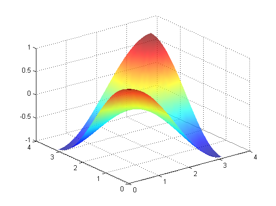
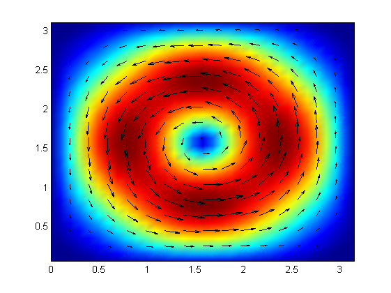
Refer to caption
(a) Pressure field
Refer to caption
(b) Velocity field
Fig. 6: Numerical results of test case 1 obtained with the SWG scheme using uniform rectangular meshes with h=1/32โ„Ž132h=1/32.

Table 1 illustrates the numerical performance of the finite difference scheme (48). The numerical velocity is clearly converging at the optimal order of r=2๐‘Ÿ2r=2 in the L2superscript๐ฟ2L^{2} norm. For the numerical pressure, the error at the cell center is decreasing at the order of r=2๐‘Ÿ2r=2, and the same conclusion can be obtained for the numerical velocity in a discrete H1superscript๐ป1H^{1} norm defined by using the cell centers. This implies that the pressure and the numerical velocity are of superconvergent to the exact solution at the center of cells. The numerical results outperforms the theoretical prediction of r=1.5๐‘Ÿ1.5r=1.5 shown in Theorem 12.

Table 1: Error and convergence performance of the finite difference scheme (48) for the Stokes equation on uniform meshes of test case 1. r๐‘Ÿr refers to the order of convergence in Oโ€‹(hr)๐‘‚superscriptโ„Ž๐‘ŸO(h^{r}).
n๐‘›n โ€–uhโˆ’uโ€–0subscriptnormsubscript๐‘ขโ„Ž๐‘ข0\|u_{h}-u\|_{0} r=๐‘Ÿabsentr= โ€–uhโˆ’uโ€–1subscriptnormsubscript๐‘ขโ„Ž๐‘ข1\|u_{h}-u\|_{1} r=๐‘Ÿabsentr= โ€–vhโˆ’vโ€–0subscriptnormsubscript๐‘ฃโ„Ž๐‘ฃ0\|v_{h}-v\|_{0} r=๐‘Ÿabsentr= โ€–vhโˆ’vโ€–1subscriptnormsubscript๐‘ฃโ„Ž๐‘ฃ1\|v_{h}-v\|_{1} r=๐‘Ÿabsentr= โ€–phโˆ’pโ€–0subscriptnormsubscript๐‘โ„Ž๐‘0\|p_{h}-p\|_{0} r=๐‘Ÿabsentr=
8 2.35e-02 0.00 5.90e-02 0.00 5.69e-02 0.00 6.61e-02 0.00 1.48e-01 0.00
16 6.26e-03 1.91 1.64e-02 1.85 1.53e-02 1.90 1.92e-02 1.78 4.29e-02 1.79
32 1.60e-03 1.97 4.25e-03 1.95 3.89e-03 1.97 5.01e-03 1.94 1.13e-02 1.92
64 4.01e-04 1.99 1.08e-03 1.98 9.78e-04 1.99 1.27e-03 1.98 2.88e-03 1.97

8.2 Test Case 2

In this test case, the analytical solution is given by

{๐’–=(โˆ’256โ€‹x2โ€‹(xโˆ’1)2โ€‹yโ€‹(yโˆ’1)โ€‹(2โ€‹yโˆ’1)256โ€‹y2โ€‹(yโˆ’1)2โ€‹xโ€‹(xโˆ’1)โ€‹(2โ€‹xโˆ’1)),p=150โ€‹(xโˆ’0.5)โ€‹(yโˆ’0.5),cases๐’–256superscript๐‘ฅ2superscript๐‘ฅ12๐‘ฆ๐‘ฆ12๐‘ฆ1missing-subexpressionmissing-subexpression256superscript๐‘ฆ2superscript๐‘ฆ12๐‘ฅ๐‘ฅ12๐‘ฅ1missing-subexpressionmissing-subexpressionmissing-subexpressionmissing-subexpressionmissing-subexpressionmissing-subexpression๐‘150๐‘ฅ0.5๐‘ฆ0.5missing-subexpressionmissing-subexpression\left\{\begin{array}[]{lll}\bm{u}=\left(\begin{array}[]{lll}-&256x^{2}(x-1)^{2}y(y-1)(2y-1)&\\ &256y^{2}(y-1)^{2}x(x-1)(2x-1)&\end{array}\right),\\ {}\\ p=150(x-0.5)(y-0.5),\end{array}\right.

and the domain is the unit square ฮฉ=(0,1)ร—(0,1)ฮฉ0101\Omega=(0,1)\times(0,1). The right-hand side function and the Dirichlet boundary data are chosen to match the exact solution. Note that this example has been considered in [9].

The numerical approximation pressure field is shown in Fig. 7(a), while the velocity vector and magnitude filds are plotted in Fig. 7(b).
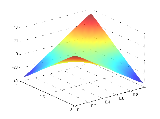
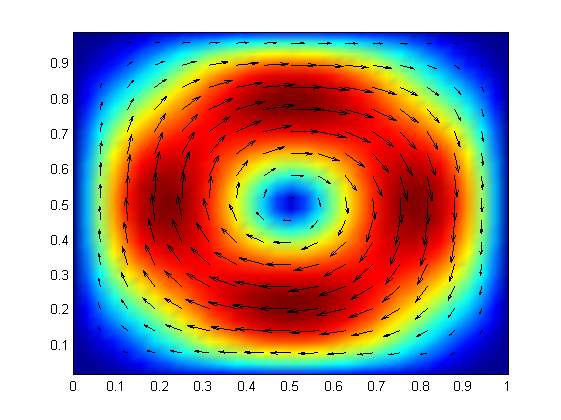
Refer to caption
(a) Pressure field
Refer to caption
(b) Velocity field
Fig. 7: Numerical results of test case 2 obtained with the SWG scheme using uniform rectangular meshes with h=1/32โ„Ž132h=1/32.

Table 2 illustrates the numerical performance of the finite difference scheme (48) for Test Case 2. It can be seen that the numerical velocity is converging at the optimal order of r=2๐‘Ÿ2r=2 in the usual L2superscript๐ฟ2L^{2} norm. For the pressure approximation, the error at the cell centers seems to be decreasing at the rate of Oโ€‹(h1.8)๐‘‚superscriptโ„Ž1.8O(h^{1.8}). It appears that the numerical velocity is also converging at the order of r=1.8๐‘Ÿ1.8r=1.8 in the discrete H1superscript๐ป1H^{1} norm defined on the cell centers. The results clearly indicate a superconvergence of the finite difference scheme for the velocity in H1superscript๐ป1H^{1} and the pressure in L2superscript๐ฟ2L^{2} on cell centers. Once again, the numerical results outperforms the theoretical prediction of r=1.5๐‘Ÿ1.5r=1.5 shown in Theorem 12.

Table 2: Error and convergence performance of the finite difference scheme (48) for the Stokes equation on uniform meshes of test case 2. r๐‘Ÿr refers to the order of convergence in Oโ€‹(hr).๐‘‚superscriptโ„Ž๐‘ŸO(h^{r}).
n๐‘›n โ€–uhโˆ’uโ€–0subscriptnormsubscript๐‘ขโ„Ž๐‘ข0\|u_{h}-u\|_{0} r=๐‘Ÿabsentr= โ€–uhโˆ’uโ€–1subscriptnormsubscript๐‘ขโ„Ž๐‘ข1\|u_{h}-u\|_{1} r=๐‘Ÿabsentr= โ€–vhโˆ’vโ€–0subscriptnormsubscript๐‘ฃโ„Ž๐‘ฃ0\|v_{h}-v\|_{0} r=๐‘Ÿabsentr= โ€–vhโˆ’vโ€–1subscriptnormsubscript๐‘ฃโ„Ž๐‘ฃ1\|v_{h}-v\|_{1} r=๐‘Ÿabsentr= โ€–phโˆ’pโ€–0subscriptnormsubscript๐‘โ„Ž๐‘0\|p_{h}-p\|_{0} r=๐‘Ÿabsentr=
8 1.03e-01 0.00 6.26e-01 0.00 7.17e-02 0.00 4.78e-01 0.00 1.39e+00 0.00
16 2.90e-02 1.82 1.97e-01 1.67 2.07e-02 1.79 1.60e-01 1.57 4.68e-01 1.58
32 7.55e-03 1.94 5.73e-02 1.78 5.43e-03 1.93 4.88e-02 1.72 1.43e-01 1.71
64 1.91e-03 1.98 1.60e-02 1.84 1.38e-03 1.98 1.41e-02 1.79 4.14e-02 1.79

8.2.1 Test Case 3: Lid driven Cavity

The lid-driven cavity problem is a benchmark test case for Stokes flow, which has been tested in many existing literatures, including [10, 12, 17, 21]. In this test case, a uniform mesh with meshsize h=1/32โ„Ž132h=1/32 is employed in our new finite difference scheme. The source term is ๐’‡=๐ŸŽ๐’‡0\bm{f}=\bm{0}, and the Dirichlet boundary condition is given as ๐’–=(1,0)T๐’–superscript10๐‘‡\bm{u}=(1,0)^{T} for y=1,xโˆˆ(0,1)formulae-sequence๐‘ฆ1๐‘ฅ01y=1,x\in(0,1) and ๐’–=(0,0)T๐’–superscript00๐‘‡\bm{u}=(0,0)^{T} on the rest of the boundary. The exact solution of lid-driven problem is not known, but the solution is known to have singularity at the corner points (0,1)01(0,1) and (1,1)11(1,1). The velocity field and streamlines are plotted in Fig. 8(a) and Fig.8(b), respectively. The pressure contour plot is shown in Fig. 9. The shape of streamlines is similar to the result given in [10, 12, 17, 21], and the results look quite reasonable.
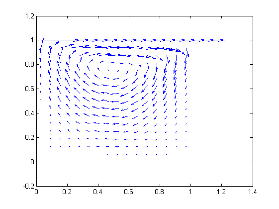
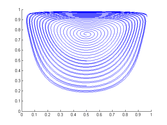
Refer to caption
(a) Velocity field
Refer to caption
(b) Streamlines
Fig. 8: Numerical results of lid-driven problem obtained with the SWG scheme using uniform rectangular meshes with h=1/32โ„Ž132h=1/32.
Refer to caption
Fig. 9: Numerical results โ€“ Pressure contours of lid-driven problem obtained with the SWG scheme using uniform rectangular meshes with h=1/32โ„Ž132h=1/32.

References

  • [1] I. Babusห˜ห˜๐‘ \breve{s}ka. The finie element method with Lagrange multipliers, Numer. Math., 20 : 173-192, 1973.
  • [2] S. Brenner and R. Scott. Mathematical theory of finite element methods, Springer, 2007.
  • [3] F. Brezzi. On the existence, uniqueness, and approximation of saddle point problems arising from Lagrange multipliers, RAIRO, 8: 129-151, 1974.
  • [4] F. Brezzi and M. Fortin. Mixed and hybrid finite element methods, Springer-Verlag, New York, 1991.
  • [5] V. Girault and P. A. Raviart. Finite element methods for Navier-Stokes equations: theory and algorithms, Springer-Verlag, Berlin, 1986.
  • [6] M D. Gunzburger. Finite element methods for viscous incompressible flows: a guide to theory, practice, and algorithms, Academic, San Diego, 1989.
  • [7] H. Han, X. Wu. A new mixed finite element formulation and the MAC method for the Stokes equations[J], SIAM Journal on Numerical Analysis, 35(2): 560-571, 1998.
  • [8] G. Kanschat. Divergence-free discontinuous Galerkin schemes for the Stokes equations and the MAC scheme[J], International journal for numerical methods in fluids, 56(7): 941-950, 2008.
  • [9] J. Li and S. Sun. The superconvergence phenomenon and proof of the MAC scheme for the Stokes equations on non-uniform rectangular meshes, Journal of Scientific Computing, 65(1): 341-362, 2015.
  • [10] M. Li, T. Tang, B. Fornberg. A compact fourth-order finite difference scheme for the steady incompressible Navier-Stokes equations. International Journal for Numerical Methods in Fluids, 20(10): 1137-1151, 1995.
  • [11] D. Li, C. Wang, J. Wang. Superconvergence of the gradient approximation for weak Galerkin finite element methods on nonuniform rectangular partitions, https://arxiv.org/pdf/1804.03998v2.pdf.
  • [12] J. Liu. Penalty-factor-free discontinuous Galerkin methods for 2-dim Stokes problems, SIAM Journal on Numerical Analysis, 49(5): 2165-2181, 2011.
  • [13] P. D. Minev. Remarks on the links between low-order DG methods and some finite-difference schemes for the Stokes problem[J]. International Journal for Numerical Methods in Fluids, 58(3): 307-317, 2008.
  • [14] R. Nicolaides. Flow discretization by complementary volume techniques[C], 9th Computational Fluid Dynamics Conference, 1989.
  • [15] J. C. Strikwerda. Finite difference methods for the Stokes and Navier-Stokes equations[J], SIAM Journal on Scientific and Statistical Computing, 5(1): 56-68, 1984.
  • [16] C. Wang and J. Wang. A primal-dual weak Galerkin finite element method for second elliptic equations in non-divergence form, Math. Comp., DOI: https://doi.org/10.1090/mcom/3220. June 2017.
  • [17] J. Wang, Y. Wang, X. Ye. A robust numerical method for Stokes equations based on divergence-free H (div) finite element methods, SIAM Journal on Scientific Computing, 31(4): 2784-2802, 2009.
  • [18] J. Wang and X. Ye. A weak Galerkin mixed finite element method for second-order ellliptic problems. available at arXiv: 1104.2897vl. J. Comp. and Appl. Math., 241, 103-115, 2013.
  • [19] J. Wang and X. Ye. A weak Galerkin mixed finite element method for second-order elliptic problems, Math. Comp., 83 (2014), pp. 2101-2126.
  • [20] J. Wang and X. Ye, A weak Galerkin finite element method for the Stokes equations. arXiv:1302.2707v1. Advances in Computational Mathematics, Volume 42, Issue 1, pp. 155-174, 2016. DOI 10.1007/s10444-015-9415-2.
  • [21] R. Wang, X. Wang, Q. Zhai, R. Zhang. A weak Galerkin finite element scheme for solving the stationary Stokes equations, Journal of Computational and Applied Mathematics, 302: 171-185, 2016.
  • [22] J. E. Welch, F. H. Harlow, J. P. Shannon, et al. The MAC method. A computing technique for solving viscous, incompressible, transient fluid-flow problems involving free surfaces, 1966.