Integrating Human-Provided Information Into Belief State Representation Using Dynamic Factorization

Abstract

In partially observed environments, it can be useful for a human to provide the robot with declarative information that represents probabilistic relational constraints on properties of objects in the world, augmenting the robot’s sensory observations. For instance, a robot tasked with a search-and-rescue mission may be informed by the human that two victims are probably in the same room. An important question arises: how should we represent the robot’s internal knowledge so that this information is correctly processed and combined with raw sensory information? In this paper, we provide an efficient belief state representation that dynamically selects an appropriate factoring, combining aspects of the belief when they are correlated through information and separating them when they are not. This strategy works in open domains, in which the set of possible objects is not known in advance, and provides significant improvements in inference time over a static factoring, leading to more efficient planning for complex partially observed tasks. We validate our approach experimentally in two open-domain planning problems: a 2D discrete gridworld task and a 3D continuous cooking task. A supplementary video can be found at http://tinyurl.com/chitnis-iros-18.

I Introduction

As robots become increasingly adept at understanding and manipulating the world around them, it becomes important to enable humans to interact with them to convey goals, give advice, or ask questions. A typical setting is a partially observed environment in which the robot has uncertainty about its surroundings, but a human can give it information to help it act more intelligently. This information could represent complex relationships among properties of objects in the world, but the robot would be expected to use it as needed when given a task or query. This setting motivates an important question: what is the best way to represent the robot’s internal knowledge so that this information is correctly processed and combined with the robot’s own sensory observations? It is important for the chosen representation to be able to accurately and efficiently answer queries (i.e. do inference) that require it to draw on the given information.

Figure 1: A schematic illustration of a dynamically factored belief. The initial belief $B$ tracks distributions over possible values for the locations of two objects. There are three locations in the world (not shown): Loc1 on the left, Loc2 in the middle, and Loc3 on the right. When the agent is given information that the objects are next to each other, the belief is updated to produce $B^{\prime}$. This is a new factoring in which the two old factors are joined into a single one, corresponding to a distribution over the joint location of both objects. Other factors (not shown) would not be affected.

We consider a specific class of open-domain planning problems in which objects exist in the world, but the agent does not know the universe of objects. We formalize our setting as a partially observable Markov decision process in which the robot has two sources of (potentially noisy) observations: its own perceptual capabilities, and assertions about the environment that simulate the human-provided information and are expressed in formal language. These observations represent constraints that hold with some probability and relate properties of objects in the world.

In order to support inference in partially observed environments, one typically maintains a belief state: a probability distribution over the space of world states. Unfortunately, the full joint distribution is usually intractable to work with. A popular alternative approach is to represent a factored belief state, in which the world state is decomposed into a set of features, each with a value. The factored belief is then a mapping from every feature to a distribution over its value.

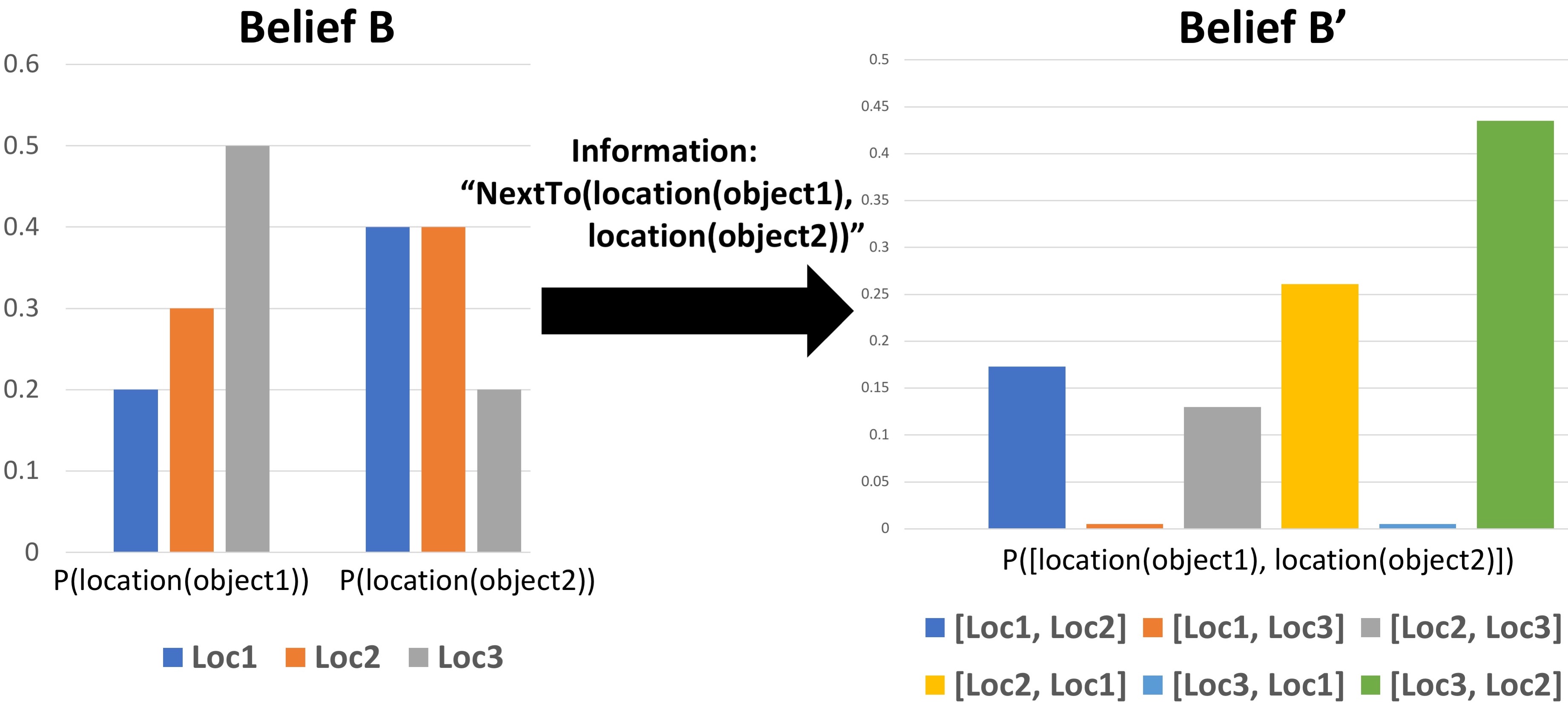
We propose a method for efficient inference using a factored belief state in the presence of potentially complicated assertions relating multiple variables. The typical approach to using a factored belief state involves committing to a (possibly domain-specific) representational choice at the very start [1, 2, 3], for which can be difficult to fold in arbitrary relational constraints without too much loss in accuracy. On the other hand, our work treats a factored belief state as a fluid, dynamic data structure in which the factoring itself is molded by the constraints, as suggested by Figure 1. We call this a dynamically factored belief.

For the class of open-domain planning problems we consider, we show that a dynamically factored belief state representation provides significant improvements in inference time over a fixed factoring. We validate our approach experimentally in two open-domain planning problems: a 2D discrete gridworld task and a 3D continuous cooking task.

Visit http://tinyurl.com/chitnis-iros-18 for a supplementary video.

II Background

II-A pomdps and Belief States

We formalize agent-environment interaction in the presence of uncertainty as a partially observable Markov decision process (pomdp) [4]. We consider a typical undiscounted setting with: $\mathcal{S}$, the state space; $\mathcal{A}$, the action space; $\Omega$, the observation space; $T(s,a,s^{\prime})=P(s^{\prime}\mid s,a)$, the transition distribution with $s,s^{\prime}\in\mathcal{S},a\in\mathcal{A}$; $O(s^{\prime},a,o)=P(o\mid s^{\prime},a)$, the observation model with $s^{\prime}\in\mathcal{S},a\in\mathcal{A},o\in\Omega$; and $R(s,a,s^{\prime})$, the reward function with $s,s^{\prime}\in\mathcal{S},a\in\mathcal{A}$. Some states in $\mathcal{S}$ are terminal, ending the episode.

At each timestep, the agent selects an action, causing 1) the hidden state to change according to $T$, 2) the agent to receive a reward according to $R$, and 3) the agent to receive an observation according to $O$. The agent’s objective is to maximize its overall expected reward, $\mathbb{E}\left[\sum_{t}R(s_{t},a_{t},s_{t+1})\right]$. A solution to a pomdp is a policy that maps the history of observations and actions to the next action to take, such that this objective is optimized over the trajectory.

The sequence of states $s_{0},s_{1},...$ is unobserved, so the agent must instead maintain a belief state: a probability distribution over the space of world states. This belief is updated on each timestep based on the received observation and taken action. The exact belief update is $B^{\prime}(s^{\prime})=\frac{1}{Z}\left[O(s^{\prime},a,o)\sum_{s\in\mathcal{S}}T(s,a,s^{\prime})B(s)\right],$ where $B$ and $B^{\prime}$ are the old and new belief states, $s^{\prime}\in\mathcal{S}$ is a state, $a\in\mathcal{A}$ is the taken action, $o\in\Omega$ is the received observation, and $Z$ is a normalizing factor.

Representing the full belief exactly is prohibitively expensive for even moderately-sized pomdps, so a typical alternative approach is to use a factored representation [2]. Here, we assume that the state can be decomposed into a set of features, each of which has a value. The factored belief is then a mapping from every feature to a distribution over its value. Typically, one chooses the features carefully so that observations can be folded, i.e. incorporated, into the belief efficiently and without too much loss of information. In other words, the chosen distributions are conjugate to the most frequent kinds of observations. Most factored representations are updated eagerly (without explicitly remembering the actions and observations) but approximately. On the other hand, a fully lazy representation just appends $a$ and $o$ to a list at each timestep. Though belief updates are trivial with this lazy representation, inference can be very expensive. In our work, we will give a representation that is sometimes eager and sometimes lazy, based on how expensive it would be to perform an eager update.

Some popular approaches for generating policies in pomdps are online planning [5, 6, 7] and finding a policy offline with a point-based solver [8, 9]. Our work will use the more efficient but more approximate determinize-and-replan approach, which optimistically plans in a determinized version of the environment, brought about by (for instance) assuming that the maximum likelihood observation is always obtained [10, 11]. The agent executes this plan and replans any time it receives an observation contradicting the optimistic assumptions made.

II-B Factor Graphs

We will be viewing our approach from the perspective of factor graphs, which we briefly describe in this section. We refer the reader to work by Kschischang et al. [12] for a more thorough treatment. A factor graph is a bipartite undirected probabilistic graphical model containing two types of nodes: variables and factors. Factor graphs provide a compact representation for the factorization of a function. Suppose a function $f$ on $n$ variables can be decomposed as $f(X_{1},X_{2},...,X_{n})=\prod_{i=1}^{m}f_{i}(C_{i}),$ where each $C_{i}\subseteq\{X_{1},X_{2},...,X_{n}\}$ is a subset of the variables. This decomposition corresponds to a factor graph in which the variables are the $X_{j}$, the factors are the $f_{i}$, and there is an edge between any $f_{i}$ and $X_{j}$ for which $X_{j}\in C_{i}$, i.e. $f_{i}$ is a function of $X_{j}$.

This representation affords efficient marginal inference, which is the process of computing the marginal distribution of a variable, possibly conditioned on the values of some other variables. Message-passing algorithms such as the sum-product algorithm typically compute marginals using dynamic programming to recursively send messages between neighboring nodes. The sum-product algorithm is also commonly referred to as belief propagation.

III Related Work

We focus on the setting of information-giving for open-domain human-robot collaboration. Information-giving was first explored algorithmically by McCarthy [13] in a seminal 1959 paper on advice-takers. Much work in open-domain collaboration focuses on the robot understanding goals given by the human [14], whereas we focus on understanding information given by the human, as in work on advice-giving [15] and commonsense reasoning [16].

III-A Adaptive Belief Representations

Our work explores belief state representations that adapt to the structure of the observations received by the robot. The work perhaps most similar to ours is that of Lison et al. [17], who acknowledge the importance of information fusion and abstraction in uncertain environments. Building on Markov Logic Networks [18], they describe a method for belief refinement that 1) groups percepts likely to be referring to the same object, 2) fuses information about objects based on these percept groups, and 3) dynamically evolves the belief over time by combining it with those in the past and future. They focus on beliefs about each object in the environment, whereas our work focuses on combining information about multiple objects, based on the structure of the observations.

The notion of adaptive belief representations has also been explored in domains outside robotics. For instance, Sleep [19] applies this idea to an acoustic target-tracking setting. The belief representation, which tracks potential locations of targets, can expand to store additional information about the targets that may be important for locating them, such as their acoustic power. The belief can also contract to remove information that is deemed no longer necessary. It would be difficult to update this factoring with information linking multiple targets, whereas our method is well-suited to incorporating such relational constraints.

III-B Factored Belief Representations for pomdps

The more general problem of finding efficient belief representations for pomdps is very well-studied. Boyen and Koller [2] were the first to provide a tractable method for belief propagation and inference in a hidden Markov model or dynamic Bayesian network. Their basic strategy is to first pick a computationally tractable approximate belief representation (such as a factored one), then after a belief update, fold the newly obtained belief into the chosen approximate representation. This technique is a specific application of the more general principle of assumed density filtering [20]. Although it seems that the approximation error will build up and propagate, the authors show that actually, the error remains bounded under reasonable assumptions. Our work adopts a fluid notion of a factored belief representation, not committing to one factoring.

Bonet and Geffner [1] introduce the idea of beam tracking for belief tracking in a pomdp. Their method leverages the fact that a problem can be decomposed into projected subproblems, allowing the joint distribution over state variables to be represented as a product over factors. Then, the authors introduce an alternative decomposition over beams, subsets of variables that are causally relevant to each observable variable. This work shares with ours the idea of having the structure of the belief representation not be fixed ahead of time. A difference, however, is that the decomposition used in beam tracking is informed by the structure of the underlying model, while ours is informed by the structure of the observations and can thus efficiently incorporate arbitrary relational constraints on the world state.

IV Formal Problem Setting

In this section, we formalize our problem setting as a pomdp, for which we will show that a dynamically factored belief is a good representation for the agent’s belief state.

Assumptions. We will assume deterministic transitions and a uniform observation model over all valid observations, in order to make progress on this difficult problem.

IV-A Planning Problem Class

We first describe the underlying class of planning problems. We consider open domains, in which the world contains a (finite or infinite) universe of objects, but the agent does not know this universe. Planning in open domains is significantly more complex than planning in settings where the universe of objects is known in advance.

The class of open-domain planning problems $\Pi$ contains tuples $\langle\mathcal{T},\mathcal{P},\mathcal{O},\mathcal{V},\mathcal{F},\mathcal{U},\mathcal{I},\mathcal{G}\rangle$:

• $\mathcal{T}$ is a known set of object types, such as locations or movables. For some types, the set of objects may be known to the agent in advance; for others, it may not.

• $\mathcal{P}$ is a known set of properties (such as color, size, pose, or contents) for each type from $\mathcal{T}$. Each property has an associated (possibly infinite) domain.

• $\mathcal{O}$ is a (possibly partially) unknown set of objects, each of a type from $\mathcal{T}$. This set $\mathcal{O}$ can be finite or infinite.

• $\mathcal{V}$ is the set of state variables resulting from applying each property in $\mathcal{P}$ to every object in $\mathcal{O}$ of the corresponding type. Each variable has a domain based on the property and can be either continuous or discrete.

• $\mathcal{F}$ is a set of fluents or constraints, Boolean-valued expressions given by a predicate applied to state variables and (possibly) values in their domains. Examples: Equal(size(obj1), 6); Different(color(obj2), color(obj3)).

• $\mathcal{U}$ is a set of object-parametrized operators that represent ways the agent can affect its environment. Each has preconditions (partial assignment of values to $\mathcal{V}$ that must hold for it to be legal), effects (partial assignment of values to $\mathcal{V}$ that holds after it is performed), and a cost.

• $\mathcal{I}$ is an assignment of values to $\mathcal{V}$ defining the initial state.

• $\mathcal{G}$ is a partial assignment of values to $\mathcal{V}$ defining the goal.

A solution to a problem in $\Pi$ is a minimum-cost sequence of parametrized operators $u_{1},...,u_{n}\in\mathcal{U}$ (a plan) such that starting with $\mathcal{I}$ and applying the $u_{i}$ sequentially satisfies operator preconditions and causes the partial assignment $\mathcal{G}$ to hold. Variables in $\mathcal{V}$ that are not in $\mathcal{G}$ may have any value.

IV-B pomdp Formulation

With $\Pi$ defined, we are ready to formulate our setting as a pomdp. Let $\langle\mathcal{T},\mathcal{P},\mathcal{O},\mathcal{V},\mathcal{F},\mathcal{U},\mathcal{I},\mathcal{G}\rangle$ be an open-domain planning problem from $\Pi$. Define the pomdp:

• $\mathcal{S}$ (the state space) is the space of all possible assignments of values to $\mathcal{V}$. A state is, thus, an assignment of a value to each variable in $\mathcal{V}$. Note that $\mathcal{I}$ is a state.

• $\mathcal{A}$ (the action space) is $\mathcal{U}$.

• $\Omega$ (the observation space) is the space of all (potentially noisy) observations: we define an observation as a set of pairs $\langle f,p\rangle$, where $f\in\mathcal{F}$ and $p\in(0,1]$. Intuitively, the interpretation is that every fluent (constraint) $f$ in this set holds with probability $p$ in the current state. We assume each observation $o$ comes from either 1) the robot’s own perceptual capabilities or 2) an assertion about the environment, which simulates human-provided information. For each fluent $f$ in $o$, the corresponding $p$ is a measure of confidence in $f$ holding within the current state. It can be based on the quality of a sensor or on the human’s certainty about the veracity of their assertion. Because $\mathcal{O}$ is unknown, a fluent may contain state variables referencing objects the agent has not encountered before.

• $T(s,a,s^{\prime})$ (the transition distribution) is 1 if $s$ satisfies $a$’s preconditions and $s^{\prime}$ its effects; 0 otherwise.

• $O(s^{\prime},a,o)$ (the observation model) is a uniform distribution over all valid observations.

• $R(s^{\prime},a)$ (the reward function) is the negative cost of $a$.

• $s\in\mathcal{S}$ is terminal, ending the episode, if $\mathcal{G}$ holds in $s$.

A solution to this pomdp is a policy that maps the history of observations and actions to the next action to take, such that the sum of expected rewards is maximized: observe that this corresponds to solving $\Pi$. Sources of uncertainty in this formulation are the open domain and the noisy observations.

Next, we present the dynamically factored belief as a good belief state representation for this pomdp. Though this representation does not depend on the presence of assertions or an open domain, we present it within this context because it best motivates the approach and manifests its strengths.

V Dynamically Factored Belief

V-A Overview

In trying to find a suitable belief state representation for the pomdp defined in the previous section, we must be cognizant of the fact that the agent does not know $\mathcal{O}$, the complete set of objects in the world. A natural representation to use might be a factored one over each state variable in $\mathcal{V}$, but unfortunately, if $\mathcal{O}$ is unknown then so is $\mathcal{V}$. Furthermore, fluents in the observations may be complicated expressions involving multiple state variables; we would like our representation to be able to incorporate these observations.

Figure 2: Example of dynamic factoring given four sequential noiseless observations in a setting with one object type and two properties: color and location. Each factor maps to a distribution over values (not shown). Initially, there are no factors. Row 1: The agent receives an assertion containing one state variable, color(A); a singleton factor for this variable is introduced. Row 2: The assertion contains two state variables, so a joint factor is introduced. Row 3: The assertion contains a new state variable, location(D), so a factor is introduced for it, then joined with the [location(B), location(C)] factor. Row 4: The agent observes the color and location of Object B. The joint distribution over the locations of B, C, and D is now uniform across the first dimension, so the factor gets split into two. This type of splitting implies that factors do not necessarily get bigger each time a new observation arrives. In this figure, all observations are noiseless (all $p=1$) for clarity of presentation. The factor graph is always a collection of independent subgraphs, where each subgraph contains exactly one factor.

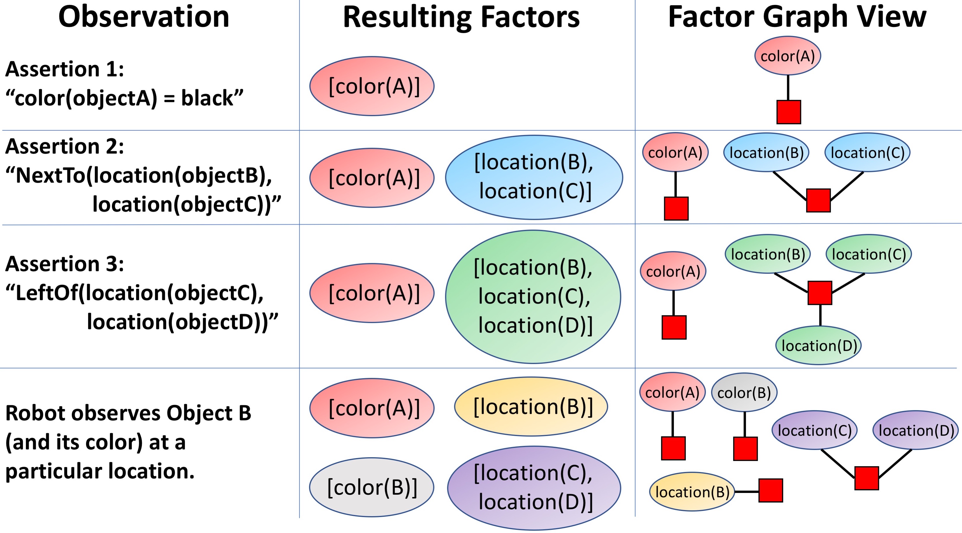
We note the following. First, we do not need to know the full set of state variables in order to maintain a (partial) factored belief representation. Second, the choice of factors should be dynamic and influenced by the observations, allowing us to gracefully cope with complicated assertions. The intuition is that a constraint linking two state variables would not be foldable into a factored representation over each state variable, so the representation should be modified. Building on these ideas, we present the following definition.

Definition 1

A dynamically factored belief state representation has two components:

• A factored representation for which each factor is a list of one or more state variables from $\mathcal{V}$. The factors partition the set of state variables that the agent knows about so far, either from prior knowledge or from a received observation. Each factor maps to a joint probability distribution over possible values for all its variables.

• A database called ComplexFluents.

The belief is initialized to have a singleton factor for each state variable in $\mathcal{V}$ associated with an object in $\mathcal{O}$ known a priori to exist, mapping to any distribution (e.g. a prior).

Each time an observation $o\in\Omega$ is received, the belief is updated as follows with every constituent fluent $f$: all factors containing state variables mentioned by $f$ are introduced (if they are not represented yet) and joined, so long as the resulting joint would not be too big. If it would be too big, then the fluent is lazily placed into ComplexFluents and considered only at query time. Furthermore, factors are regularly split up for efficiency, implying that a belief update could potentially compress the representation. This is shown in Figure 2 and described in detail in the next section. Newly introduced variables can map to any distribution, such as a uniform one, or one calculated from some prior knowledge.

The factors partition the set of state variables that the agent knows about so far, meaning no state variable can ever be present in more than one factor. Enforcing this invariant greatly simplifies inference, as can be understood from a factor graph perspective. A dynamically factored belief maintains a factor graph with variable nodes $V$ and factor nodes $F$, where the $V$ are the state variables in $\mathcal{V}$ that the agent knows about so far, and the $F$ are the factors. Each node $F$ connects to all the $V$ that are present in the corresponding list (and thus comprise that factor’s joint distribution). Because the factors partition the variables, this factor graph is a collection of independent subgraphs, where each subgraph contains exactly one node from $F$ connected to one or more nodes from $V$. See Figure 2 for an example. Fluents placed lazily into ComplexFluents are not part of this factor graph. The structure of this factor graph is constantly changing as new objects are discovered and observations are received, but it will always be a collection of independent subgraphs. Thus, there is no possibility of ending up with a cyclic factor graph, which would typically necessitate either approximate inference or expensive exact inference.

Note. All fluents, complex or not, can be represented by a factor in some more complex factor graph. One could imagine a different algorithm that avoids constructing the joint of all variables mentioned by a fluent, but instead creates a new factor for the fluent while leaving other factors untouched. This would likely create cycles, but cycles could be collapsed into joint distributions over all constituent nodes. Inference would then be done using message-passing. In contrast, our method eagerly incorporates fluents in a way that makes inference fast and cycles impossible. Furthermore, our method can very quickly answer queries about a marginal on a subset of any factor, as we will see.

V-B Belief Update Algorithm

Algorithm Dynamically Factored Belief Update

      1 $B\leftarrow$ InitializeFactoredBeliefMap()

      2 ComplexFluents $\leftarrow$ set({})

       Subroutine BeliefUpdate(observation, action)

            3 for each $\langle f,p\rangle$ in observation do

                  4 for each stateVar mentioned by $f$ do

                        5 if !$B$.Contains(stateVar) then

                              6 $B$.Add([stateVar], defaultDist())

                              

                  7if joint would be too big then

                        8 ComplexFluents.Add($f$)

                        

                  else

                        9 $B$.JoinFactorsAndUpdate($f,p$)

            10$B$.UpdateWithAction(action)

             // Keep representation compact.

            11 for each factor in $B$.Factors do

                  12 $B$.TrySplit(factor, $\epsilon$)

                  

Algorithm 1 Dynamically factored belief update.

Algorithm 1 gives pseudocode for updating a dynamically factored belief. The belief is initialized to contain a singleton factor for each state variable in $\mathcal{V}$ associated with an object in $\mathcal{O}$ known a priori to exist. The BeliefUpdate subroutine is called at each timestep, after the agent takes an action and receives an observation (a set of fluents, each with a corresponding probability of holding in the world).

Line 7 decides whether joining all factors containing a state variable mentioned by the fluent would result in a joint that is too “big” (expensive to compute or represent). If so, the fluent is lazily stored in the database ComplexFluents and considered only at query time. An implementation of this test could take the product of the factor sizes and check whether it is above a certain threshold.

Subroutine JoinFactorsAndUpdate($B,f,p$)

      1 joint $\leftarrow$ (join factors $F$ containing variables in $f$)

      2 $m\leftarrow$ (total prob. of values inconsistent with $f$)

      3 for each value in joint do

            4 if value is inconsistent with $f$ then

                  5 joint.RescaleProbBy$\left(\text{value},\frac{(1-p)(1-m)}{pm}\right)$

                  

      6joint.Normalize()

      7 Add joint to $B$ and remove all $F$ from $B$.

      

Subroutine TrySplit($B$, factor, $\epsilon$)

      8 for each state variable $V$ in factor do

            9 reconstructed $\leftarrow$ Join($B$[V], $B$[factor $\setminus$ {V}])

            10 if $D_{JS}(B[\text{factor}]\;\|\;\text{reconstructed})<\epsilon$ then

                  11 Split $B$[factor] into $B$[V], $B$[factor $\setminus$ {V}].

                  

Algorithm 2 Subroutines used in Algorithm 1.

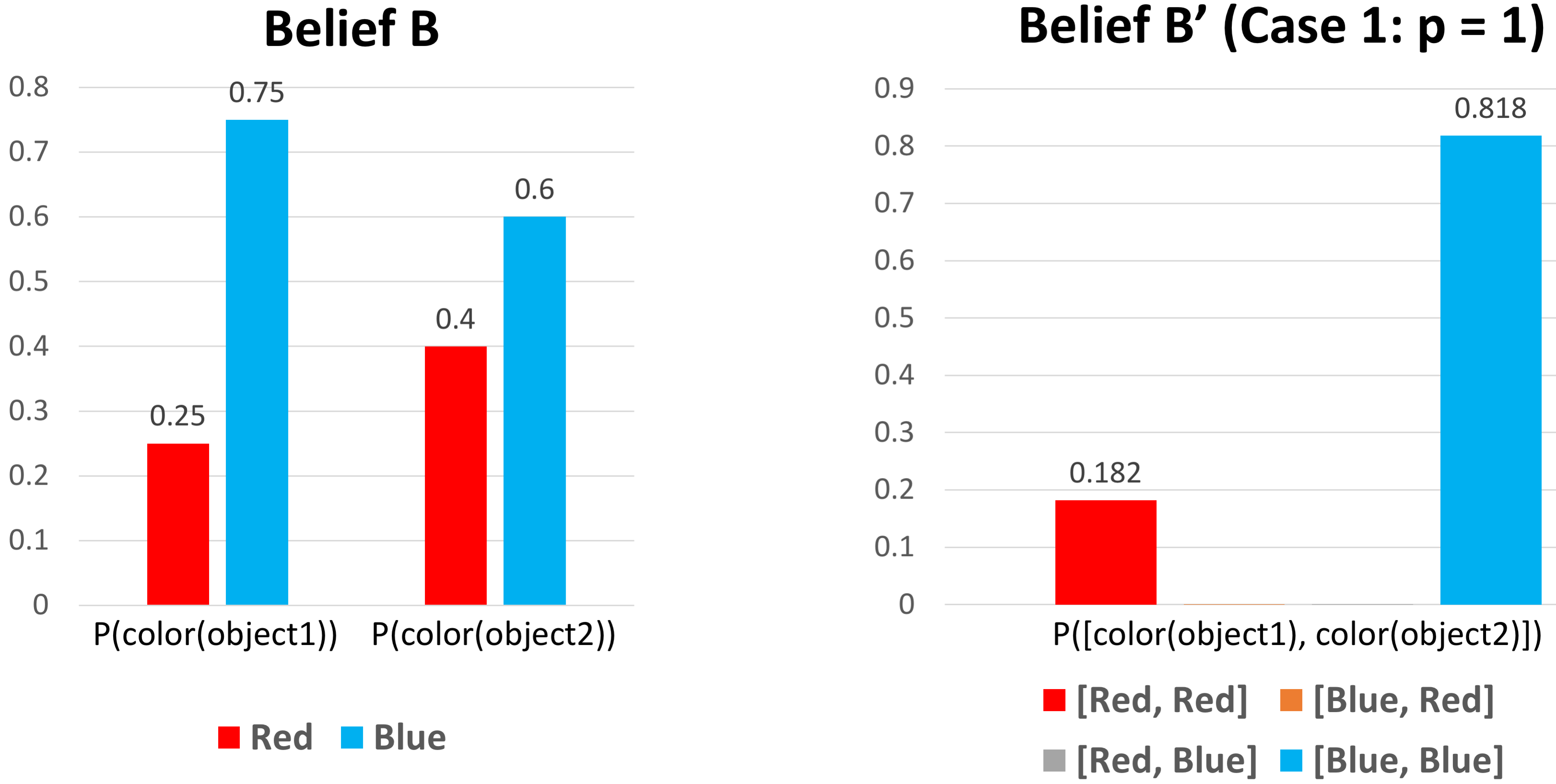
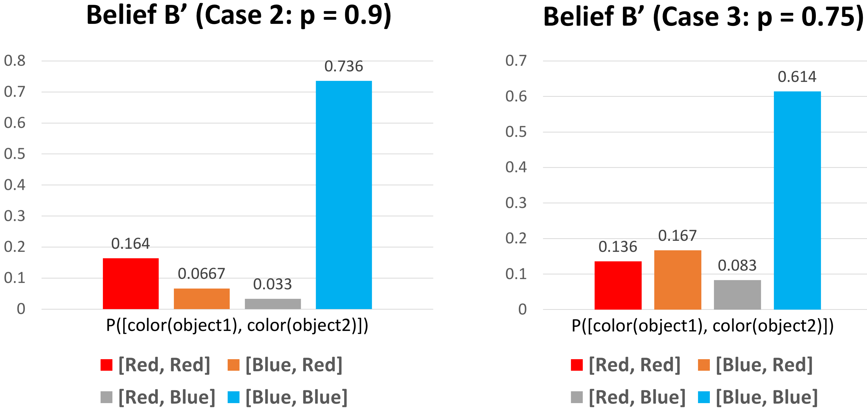
Joining Factors  The call in Line 9 to JoinFactorsAndUpdate creates a new factor containing all state variables that are mentioned by the fluent $f$ (if such a factor is not already present), then maps this factor to a joint distribution for which $f$ holds with probability $p$. To accomplish this, we build the joint then rescale the probabilities such that $p$ mass goes to the joint values which are consistent with $f$, and the remaining $1-p$ mass goes to those which are inconsistent. This can be done using Jeffrey’s rule [21]: rescale the probability of all values inconsistent with $f$ by $\frac{(1-p)(1-m)}{pm}$, where $m$ is the total probability of these inconsistent values, then normalize. When $p=1$, this algorithm just filters out joint values inconsistent with $f$, as expected. See Algorithm 2 for pseudocode and Figure 3 for an example. If distributions are continuous, we perform these operations implicitly using rejection sampling at query time.

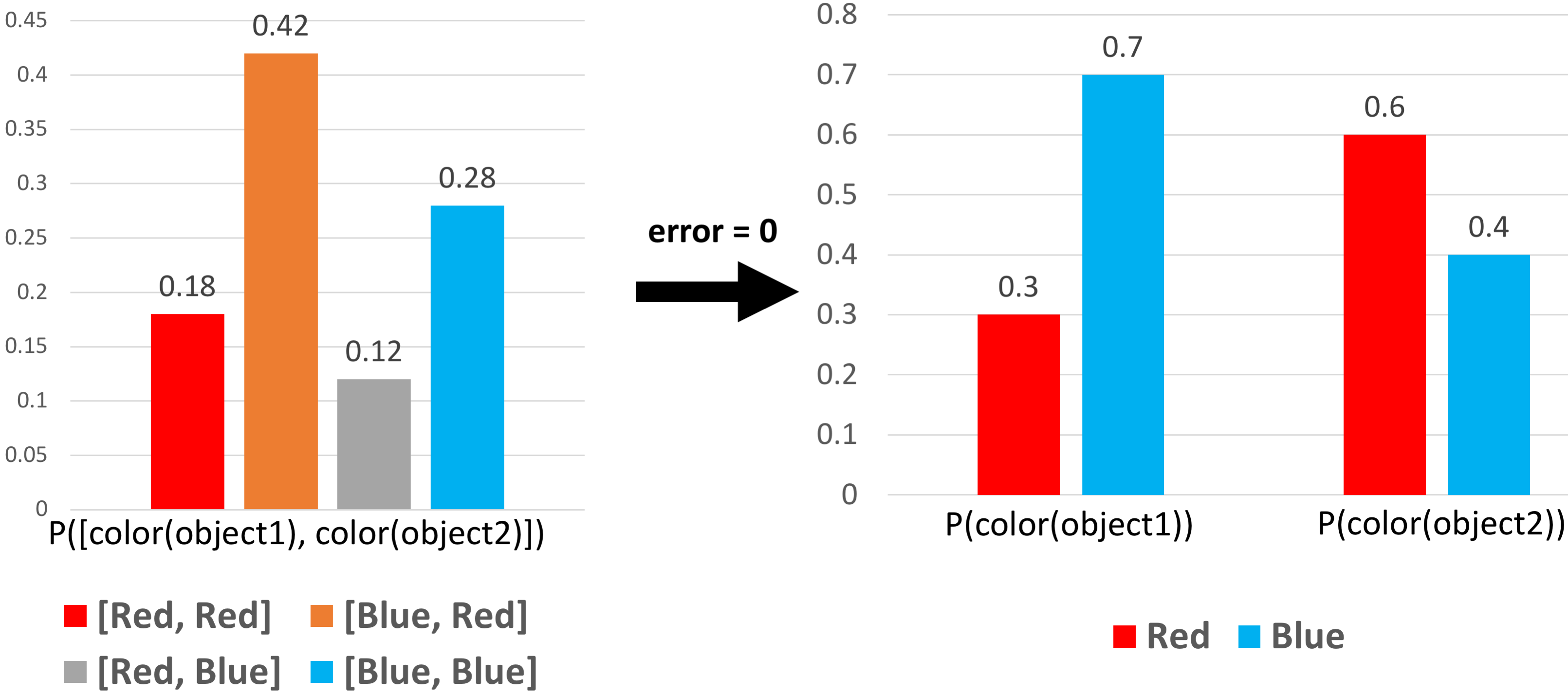
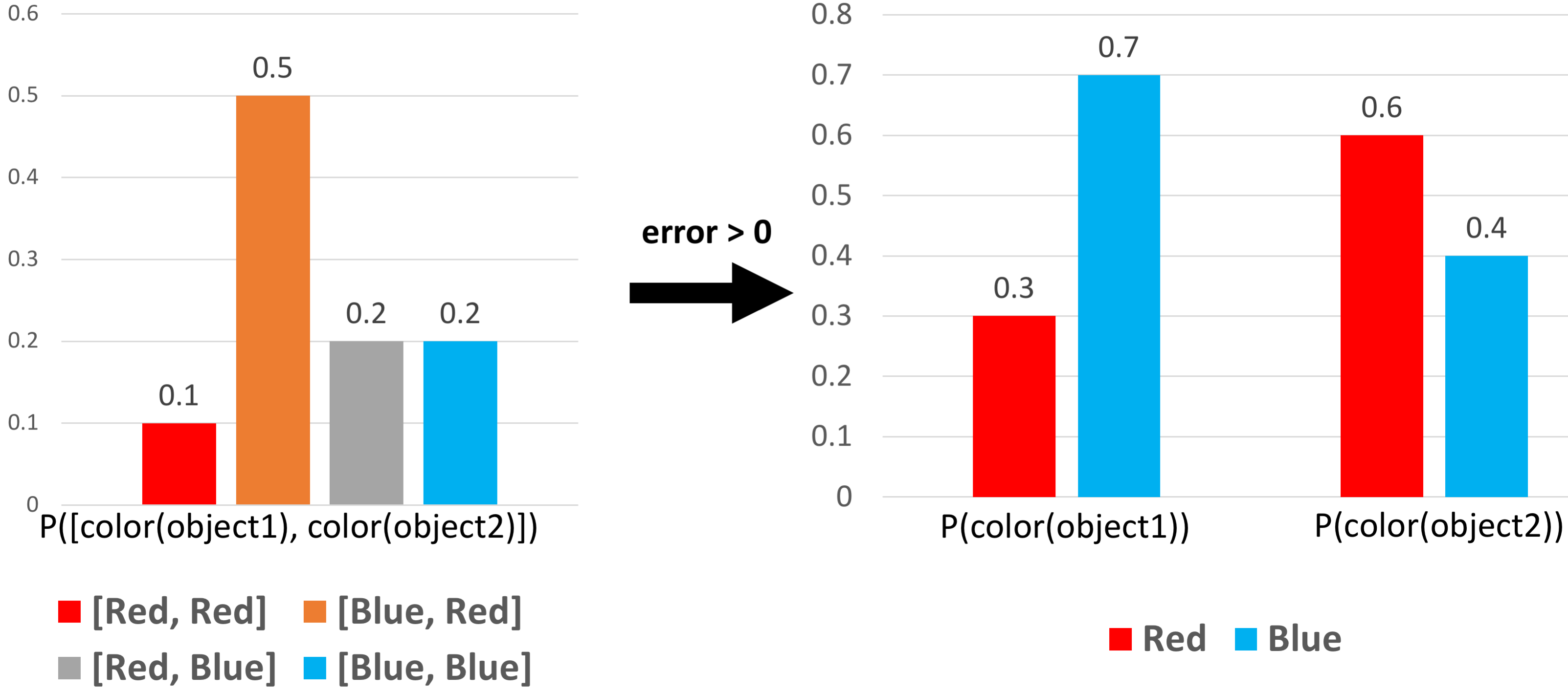
Splitting Factors  The call in Line 12 to TrySplit attempts to split up factors to maintain a compact representation. In practice, we accomplish this by checking whether each state variable in the factor can be marginalized out. Of course, it is unlikely that such marginalization can ever be done in a lossless manner, as this would require the joint to be exactly decomposable into a product involving this marginal. Instead, we perform marginalization whenever the reconstruction error is less than a hyperparameter $\epsilon$. We measure this reconstruction error as the Jensen-Shannon divergence $D_{JS}$ between the true joint and the approximate joint reconstructed from the attempted decomposition.

Let $P$ and $Q$ be arbitrary probability distributions. The Jensen-Shannon divergence is a smooth, symmetric, bounded measure of similarity between $P$ and $Q$. It is based on the Kullback-Leibler (KL) divergence, defined as $D_{KL}(P\;\|\;Q)=-\sum_{i}P(i)\log\frac{Q(i)}{P(i)},$ where the summation can be replaced by integration for continuous distributions. Then letting $A=\frac{1}{2}(P+Q)$, the Jensen-Shannon divergence is defined as $D_{JS}(P\;\|\;Q)=\frac{1}{2}D_{KL}(P\;\|\;A)+\frac{1}{2}D_{KL}(Q\;\|\;A).$ Assuming the natural logarithm is used, the bound $0\leq D_{JS}(P\;\|\;Q)\leq\log 2$ always holds. Since $D_{JS}$ is bounded, it is reasonable to use $\epsilon$ as a fixed threshold on the reconstruction error to decide whether to do marginalization. Varying $\epsilon$ lets the designer trade off between compactness of the belief and accuracy of inference. See Algorithm 2 for pseudocode and Figure 4 for an example.

Figure 3: Posteriors from running JoinFactorsAndUpdate with fluent Same(color(object1), color(object2)), for three values of $p$.

Figure 4: Two examples of trying to split up a factor having two variables. Top: The variables are independent; no error is incurred. Bottom: Error is incurred based on the Jensen-Shannon divergence between the joint and the product of the marginals ($\sim$0.01 here).

V-C Inference

Dynamically factored beliefs can handle two types of queries: 1) a marginal on any state variable, or on a set of state variables that is a subset of some factor, and 2) a sample from the full joint of current factors, which gives a world state consistent with the agent’s current knowledge.

To answer queries of type 1), we observe that if a state variable or set of state variables is a subset of some factor, then our representation already stores a joint distribution over values for those variables. Any query about them can be answered using this joint, e.g. by sampling. We do not have to worry about violating the constraints in ComplexFluents because each of those could only ever constrain a set of state variables that spans multiple factors.

To answer queries of type 2), we must draw from the distribution implicitly encoded by all factors together, which produces an assignment that maps every currently known state variable to a value. One can treat this as a constraint satisfaction problem [22] where the constraints are the fluents in ComplexFluents (all other fluents have already been folded eagerly into the belief), and apply standard solving techniques. Our experiments solve it incrementally using a backtracking approach; see Algorithm 3 for pseudocode.

Algorithm SampleState($B$, ComplexFluents)

      1 state $\leftarrow$ map(each state variable in $B\to$ NULL)

      2 curIndex $\leftarrow$ 0

      3 while curIndex $<$ number of factors do

            4 factor $\leftarrow$ $B$.Factors[curIndex]

            5 if sampling limit reached then

                  6 for each stateVar in factor do

                        7 state[stateVar] $\leftarrow$ NULL

                  8curIndex $\leftarrow$ curIndex $-$ 1

                   continue

            9values $\leftarrow B$[factor].Sample()

            10 for stateVar, value in zip(factor, values) do

                  11 state[stateVar] $\leftarrow$ value

            12if any $f$ in ComplexFluents cannot hold then

                  continue

            13curIndex $\leftarrow$ curIndex + 1

            

      return state

Algorithm 3 An incremental algorithm for sampling a world state consistent with all observations, using a dynamically factored belief $B$. The returned state is an assignment of currently known state variables to values.

VI Experiments

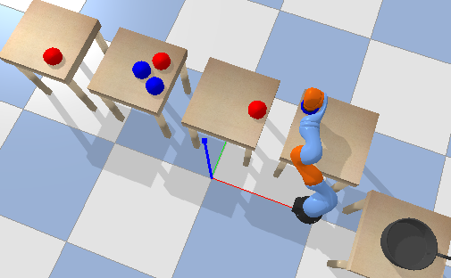
We evaluate the performance of our approach on the cooking task, a planning problem from $\Pi$. The robot is tasked with gathering ingredients and using them to cook a meal. There are three object types: $\mathcal{T}=\{$locations, vegetables, seasonings$\}$. The term ingredients refers to vegetables and seasonings together. Each object type has one property. Locations have a contents property, which is one of “vegetable,” “seasoning,” or “empty.” Ingredients have a position property, which could be continuous- or discrete-valued. Initially, the robot knows the set of locations but not the set of ingredients. There is a pot at a fixed, known position.

When any vegetable is placed into the pot, it transitions to a cooking state; 5 timesteps later, it transitions to a cooked state. The goal is to have all ingredients in the pot and all vegetables cooked. However, the robot is penalized heavily for placing any seasoning into the pot too early, before all vegetables have been cooked. To achieve the goal, the robot must learn the positions of all ingredients, either by doing observations or by learning about them from assertions.

The operators (actions) $\mathcal{U}$ are:

• Observe(location): Moves and observes the ingredient(s) at a location. Cost: 5.

• Pick(position): Moves and picks at a continuous- or discrete-valued position (domain-dependent). The robot can hold up to 10 ingredients at once. Cost: 20.

• PlaceInPot(): Places all $n$ held ingredients into the pot. Vegetables in the pot are either cooking or, 5 timesteps later, cooked. Cost: 100 + 50$n$, plus an additional 1000 if a seasoning is placed in before all vegetables are cooked.

• No-op(): Takes no action. Cost: 0.

There is also a living cost of 10 per timestep.

The state variables $\mathcal{V}$ comprise each location’s contents and each ingredient’s position. The world state contains an assignment of these variables to values. It also tracks which ingredients are held by the robot and the pot, and the current robot pose; these are all assumed to be known and thus do not need to be tracked by the belief state.

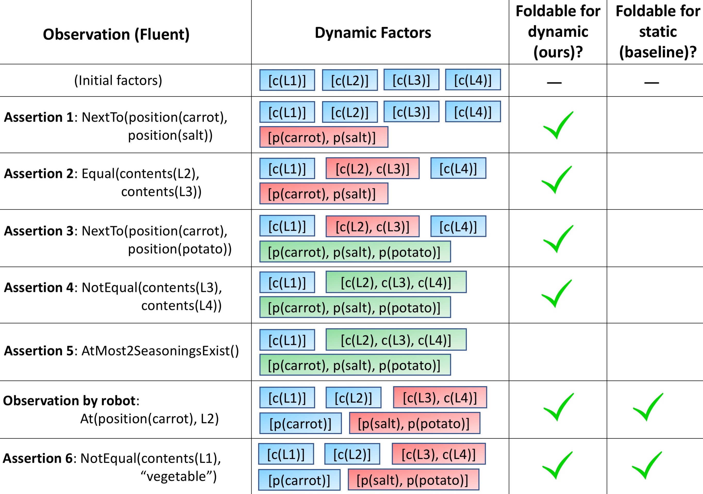
Assertions. Figure 5 shows the types of assertions we use. At each timestep, we sample an assertion uniformly at random from all valid ones, following our observation model, and give it to the robot. The information could be redundant.

Figure 5: An illustration of the types of assertions we use, with a simplified execution of the gridworld cooking task. There are four locations: L1, L2, L3, L4. Factors are color-coded based on the number of state variables. c($\cdot$) means contents($\cdot$), p($\cdot$) means position($\cdot$). Initially, there is a singleton factor for each location’s contents. The last two columns tell whether the fluent is foldable into a dynamic factoring (our approach), and into a static factoring that tracks the potential contents of each location (baseline). Unfoldable fluents get placed into ComplexFluents, slowing down inference. Observe that singleton factors go in and out of joints.

Baseline. We test against a baseline belief representation that simulates prior work on factored representations, which typically commit to a representational choice at the start. This baseline, which we call a statically factored belief or static factoring, represents the agent’s belief as a distribution over the potential contents of each location. The factoring does not change based on observations, or as ingredients are discovered. We choose this factoring as our baseline because initially, the robot only knows the set of locations, not the set of ingredients. Thus, this factoring is the most reasonable choice for a static representation that is chosen at the start and held fixed throughout execution. Any fluent that cannot fold into this static factoring is lazily placed into ComplexFluents and considered only at query time.

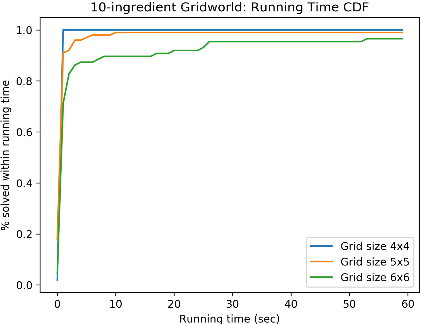
Domain 1: Discrete 2D Gridworld Cooking Task  Our first experimental domain is the cooking task in a 2D gridworld. Locations are organized in a 2D grid, and the robot is in exactly one at any time. Both Observe and Pick actions are performed on single grid locations. Each location is initialized to contain either a single ingredient or nothing, so the position property of each ingredient is a discrete value corresponding to a location. We solve the task using the determinize-and-replan approach to belief space planning, with A* as the planner. The task is computationally challenging, so we impose a 60-second timeout per episode.

Domain 2: Continuous 3D Cooking Task  Our second experimental domain is the cooking task in a pybullet simulation [23]. Here, the position property of each ingredient is a continuous value: each can be placed anywhere on the surface of one of four tables. The robot can Observe any table and Pick at any position along a table surface, so the action space is continuous. Locations are given by a grid discretization of the environment geometry. As ingredients get discovered, a dynamically factored belief adapts to track continuous distributions over their positions. Again, we use the determinize-and-replan method and a 60-second timeout.

Setting	System	% Solved	Bel. Upd. Time	Queries / Second
Dom. 1, 4x4, 6ing	S (baseline)	67	0.01	0.11
Dom. 1, 4x4, 6ing	D (ours)	100	0.03	20
Dom. 1, 4x4, 10ing	S (baseline)	50	0.01	0.068
Dom. 1, 4x4, 10ing	D (ours)	100	0.04	16.7
Dom. 1, 5x5, 6ing	S (baseline)	13	0.01	0.039
Dom. 1, 5x5, 6ing	D (ours)	100	0.06	2.27
Dom. 1, 5x5, 10ing	S (baseline)	5	0.01	0.031
Dom. 1, 5x5, 10ing	D (ours)	99	0.08	2.3
Dom. 1, 6x6, 6ing	S (baseline)	5	0.01	0.019
Dom. 1, 6x6, 6ing	D (ours)	100	0.13	1.15
Dom. 1, 6x6, 10ing	S (baseline)	5	0.01	0.028
Dom. 1, 6x6, 10ing	D (ours)	97	0.23	0.338
Dom. 2, 8ing	S (baseline)	55	0.07	0.495
Dom. 2, 8ing	D (ours)	100	0.11	5.56
Dom. 2, 10ing	S (baseline)	48	0.07	0.287
Dom. 2, 10ing	D (ours)	100	0.14	4.76

TABLE I: Some of our experimental results. Each row reports averages over 100 independent episodes. Percentage of tasks solved within 60-second timeout, belief update time (seconds), and average number of queries answered per second (across solved tasks) are shown. S: Statically factored belief (baseline), D: Dynamically factored belief (our method). Setting column gives domain (“Dom. 1” is gridworld, “Dom. 2” is continuous), grid size (if applicable), and number of ingredients. Our approach solves more tasks than a static factoring does, and inference is an order of magnitude faster.

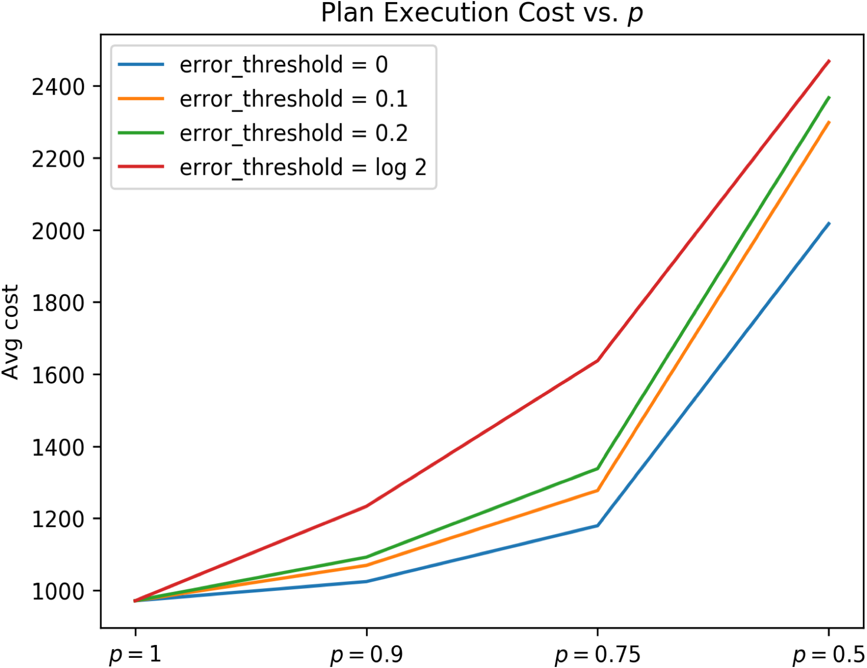
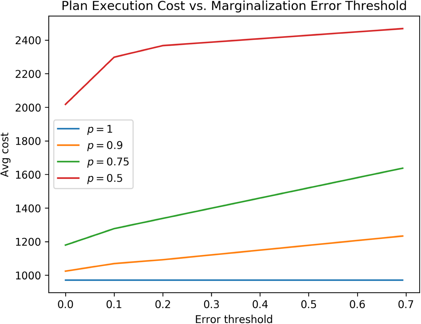
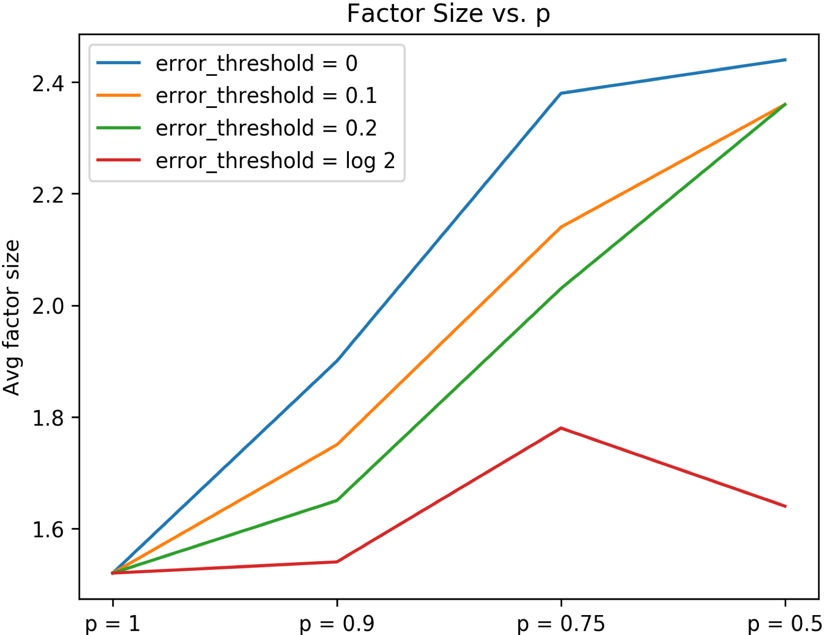
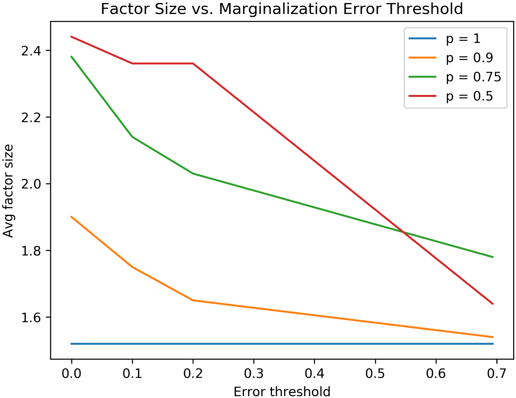
Results and Discussion  Table I and Figure 6 show results when all $p$ are 1 and $\epsilon$ is 0 (see Algorithm 2), while Figure 7 shows results with noisy observations where $p$ and $\epsilon$ vary. Overall, our approach solves significantly more tasks than a static factoring does, and also does inference an order of magnitude faster. However, our method could perform badly when belief updates are very expensive, which could happen if we try to eagerly incorporate fluents that link several state variables with large domains. Typically in practice, though, such fluents would be placed into ComplexFluents. As $p$ decreases, observations get noisier, so execution costs and factor sizes increase. As $\epsilon$ increases, more marginalization occurs and inference accuracy is lower, so factors are smaller but execution is costlier.

Figure 6: Left: Cumulative distribution functions showing the percentage of the 100 episodes we ran with our method that got solved within different running times, for the 10-ingredient gridworld. Although our timeout was set to 60 seconds, most tasks were solved within 10 seconds, whereas the baseline (not shown) timed out frequently (see Table I). Right: A visualization of the continuous 3D cooking domain. The robot is a light-blue-and-orange arm. Vegetables (red) and seasonings (blue) are placed across four tables.

Figure 7: Results for varying $p$ and $\epsilon$ (see Algorithm 2) in our experiments. As $p$ decreases, observations get noisier, so execution costs and factor sizes increase. As $\epsilon$ increases, more marginalization occurs (with reconstruction error) and inference accuracy decreases, so factors are smaller but execution is costlier.

VII Conclusion and Future Work

We have considered the problem of belief state representation in an open-domain planning problem where a human can give relational information to the robot. We showed that a dynamically factored belief is a good representational choice for efficient inference and planning in this setting.

One future direction to explore is to approximately fold information into the belief representation rather than compute a joint on every update. We should seek a mechanism that allows the designer to trade off between compactness of the belief and accuracy of inference. Another direction to explore is a non-uniform observation model: a robot given information $I$ can learn something not only from $I$ but also from the fact that it was told $I$ as opposed to anything else.

References

- [1] B. Bonet and H. Geffner, “Belief tracking for planning with sensing: Width, complexity and approximations,” Journal of Artificial Intelligence Research, 2014.
- [2] X. Boyen and D. Koller, “Tractable inference for complex stochastic processes,” in Proceedings of the Fourteenth Conference on Uncertainty in Artificial Intelligence, 1998.
- [3] B. Sallans, “Learning factored representations for partially observable Markov decision processes,” in Advances in neural information processing systems, 2000, pp. 1050–1056.
- [4] L. P. Kaelbling, M. L. Littman, and A. R. Cassandra, “Planning and acting in partially observable stochastic domains,” Artificial intelligence, vol. 101, pp. 99–134, 1998.
- [5] D. Silver and J. Veness, “Monte-carlo planning in large POMDPs,” in Advances in neural information processing systems, 2010, pp. 2164–2172.
- [6] A. Somani, N. Ye, D. Hsu, and W. S. Lee, “DESPOT: Online POMDP planning with regularization,” in Advances in neural information processing systems, 2013, pp. 1772–1780.
- [7] B. Bonet and H. Geffner, “Planning with incomplete information as heuristic search in belief space,” in Proceedings of the Fifth International Conference on Artificial Intelligence Planning Systems, 2000, pp. 52–61.
- [8] H. Kurniawati, D. Hsu, and W. S. Lee, “SARSOP: Efficient point-based POMDP planning by approximating optimally reachable belief spaces.” in Robotics: Science and systems, vol. 2008. Zurich, Switzerland., 2008.
- [9] J. Pineau, G. Gordon, S. Thrun et al., “Point-based value iteration: An anytime algorithm for POMDPs,” in IJCAI, vol. 3, 2003, pp. 1025–1032.
- [10] R. Platt Jr., R. Tedrake, L. Kaelbling, and T. Lozano-Perez, “Belief space planning assuming maximum likelihood observations,” 2010.
- [11] D. Hadfield-Menell, E. Groshev, R. Chitnis, and P. Abbeel, “Modular task and motion planning in belief space,” in Intelligent Robots and Systems (IROS), 2015 IEEE/RSJ International Conference on, 2015, pp. 4991–4998.
- [12] F. R. Kschischang, B. J. Frey, and H.-A. Loeliger, “Factor graphs and the sum-product algorithm,” IEEE Transactions on information theory, vol. 47, no. 2, pp. 498–519, 2001.
- [13] J. McCarthy, Programs with common sense. RLE and MIT Computation Center, 1959.
- [14] K. Talamadupula, J. Benton, S. Kambhampati, P. Schermerhorn, and M. Scheutz, “Planning for human-robot teaming in open worlds,” ACM Transactions on Intelligent Systems and Technology (TIST), vol. 1, no. 2, p. 14, 2010.
- [15] P. Odom, T. Khot, and S. Natarajan, “Learning probabilistic logic models with human advice,” in 2015 AAAI Spring Symposium Series, 2015.
- [16] S. Zhang and P. Stone, “CORPP: Commonsense reasoning and probabilistic planning, as applied to dialog with a mobile robot.” in AAAI, 2015, pp. 1394–1400.
- [17] P. Lison, C. Ehrler, and G. J. M. Kruijff, “Belief modelling for situation awareness in human-robot interaction,” in 19th International Symposium in Robot and Human Interactive Communication, 2010.
- [18] M. Richardson and P. Domingos, “Markov logic networks,” Machine learning, vol. 62, no. 1, pp. 107–136, 2006.
- [19] S. R. Sleep, “An adaptive belief representation for target tracking using disparate sensors in wireless sensor networks,” in Proceedings of the 16th International Conference on Information Fusion, 2013.
- [20] P. S. Maybeck, Stochastic models, estimation, and control. Academic press, 1982, vol. 3.
- [21] R. C. Jeffrey, The logic of decision. University of Chicago Press, 1965.
- [22] R. Dechter and D. Cohen, Constraint processing. Morgan Kaufmann, 2003.
- [23] E. Coumans, Y. Bai, and J. Hsu, “Pybullet physics engine,” 2018. [Online]. Available: http://pybullet.org/