Davydov-Type Excitonic Effects on the Absorption Spectra of Parallel-Stacked and Herringbone Aggregates of Pentacene: Time-Dependent Density-Functional Theory and Time-Dependent Density-Functional Tight Binding

Abstract

Exciton formation leads to J-bands in solid pentacene. Describing these exciton bands represents a challenge for both time-dependent (TD) density-functional theory (DFT) and for its semi-empirical analogue, namely for TD density-functional tight binding (DFTB) for three reasons: (i) solid pentacene and pentacene aggregates are bound only by van der Waals forces which are notoriously difficult to describe with DFT and DFTB, (ii) the proper description of the long-range coupling between molecules, needed to describe Davydov splitting, is not easy to include in TD-DFT with traditional functionals and in TD-DFTB, and (iii) mixing may occur between local and charge transfer excitons, which may, in turn, require special functionals. We assess how far TD-DFTB has progressed towards a correct description of this type of exciton by including both a dispersion correction for the ground state and a range-separated hybrid functional for the excited state and comparing the results against corresponding TD-CAM-B3LYP/CAM-B3LYP+D3 results. Analytic results for parallel-stacked ethylene are derived which go beyond Kasha’s exciton model [Kasha, Rawls, and El-Bayoumi, Pure Appl. Chem. 11, 371 (1965)] in that we are able to make a clear distinction between charge transfer and energy transfer excitons. This is further confirmed when it is shown that range-separated hybrids have a markedly greater effect on charge-transfer excitons than on energy-transfer excitons in the case of parallel-stacked pentacenes. TD-DFT calculations with the CAM-B3LYP functional and TD-lc-DFT calculations lead to negligeable excitonic corrections for the herringbone crystal structure, possibly because of an overcorrection of charge-transfer effects. In this case, TD-DFT calculations with the B3LYP functional or TD-DFTB calculations parameterized to B3LYP give the best results for excitonic corrections for the herringbone crystal structure as judged from comparison with experimental spectra and with Bethe-Salpeter equation calculations from the literature.

I Introduction

Organic electronics Müllen and Scherf (1990); Pope and Swenberg (1999); Jain et al. (2007); Anthony (2008); Agranovich (2009) has emerged in recent years as an important niche market, notably for organic light emitting diodes used in lighting, television, computer, and telephone display screens, and for organic solar cells. Part of the appeal of organic electronics is the ease of design of new materials via tools from the organic chemist’s large and diverse toolbox and the ease of fabrication of “plastic” and “printable” electronics. At the heart of the functioning of organic electronic devices are energy-transfer (ET) and charge-transfer (CT) processes May and Kühn (2000) whose understanding could benefit from better modeling. However the size and complexity of organic materials and the need to treat electonic excited states puts severe limitations on the modeling methods that can be used. These limitations become even more severe if the goal is to model exciton dynamics or charge transport. Even standard methods for “large” systems such as density-functional theory (DFT) and time-dependent (TD) DFT may need to be approximated by their semi-empirical analogues, notably by density-functional tight-binding (DFTB) and TD-DFTB, in order to treat large-enough systems to be of practical interest in organic electronics. Moreover “ordinary” DFT(B) and TD-DFT(B) is not good enough for treating organic molecular solids and excitations in these systems because of the need for at least a minimally-correct treatment of van der Waals (vdW) forces and CT excitations. In this article, we evaluate the ability of TD-DFTB and of state-of-the-art TD long-range corrected (lc) DFTB to simulate the results of TD-B3LYP and TD-CAM-B3LYP calculations for describing exciton structure in the spectra of pentacene aggregates. In the process, we revisit Kasha’s exciton model Kasha et al. (1965), which is often used in analyzing experimental results, and point out some of its strengths and weaknesses.

Organic materials are typically bound together by some combination of hydrogen bonding and vdW forces. In the case of pentacene, the forces binding the molecules together are purely vdW in nature. It is thus imperative to be able to include dispersion forces. Traditional density functionals, such as the local density approximation (LDA), generalized gradient approximations (GGAs), meta-GGAs, and hybrid functionals fail to include the “action at a distance” aspect of dispersion forces because of their inability to give an accurate description of forces between molecules with nonoverlapping densities. Perhaps ironically, $C_{6}$ van der Waals coefficients — and hence dispersion forces — may be calculated accurately by TD-DFT. At this time, the most popular way to include dispersion forces in DFT calculations is to add on a semi-empirical correction Grimme et al. (2010) which is designed to interpolate between the DFT description of the charge density and the TD-DFT description of $C_{6}$ coefficients.

Organic electronics relies upon charge transport. However positive and negative carriers may be transported together in a charge-neutral packet called an exciton. From the condensed-matter point of view, excitons are born as local excitations. In fact, it is useful to make a distinction between “exciton structure” and “exciton dynamics” (p. 5 Ref. Knox (1963)). Although related to each other, exciton structure is more directly related to absorption spectra — the subject of the present article — while exciton dynamics falls more conveniently under the heading of charge and energy transport May and Kühn (2000). Even within the seemingly narrow subject of exciton structure, excitons seem to mean different things to different people. In particular, solid-state physicists may seem to require periodic (crystal) boundary conditions Knox (1963) in their definition of excitons, while chemists Kasha (1959); Kasha et al. (1965) and biochemists van Amerongen et al. (2000) do not.

An important distinction between solids and molecules has to do with what we informally call the “size of a photon.” In the usual way of thinking, monochromatic light has a well-defined momentum and hence, by Heisenberg’s well-known uncertainty principle, must be infinitely delocalized in space. The theory of molecular spectroscopy is almost (but not really) contradictory regarding the size of the photon in the sense that it usually assumes monochromatic light modeled by an electronic field at fixed frequency, but one whose interaction with the molecule is sufficiently sudden to be able to use Fermi’s golden rule. That is, the moleule is small compared to the size of of the photon but the photon interacts with the molecule for only a short period of time while it passes by.

Here we focus on molecular solids where intermolecular interactions are important. Frenkel introduced the term “excitation packets” in his early study of the conversion of light into heat in solids Frenkel (1931, 1932). Unlike molecules which may often be considered to be small enough compared to the size of a photon that the photon may be approximated by an oscillating electric field, a solid is large compared to a photon. In particular, solids typically only interact locally with light, say, only near the surface where illuminated by a laser beam. Yet the crystal molecular orbitals should in principle extend over the entire crystal and so must also be large compared to the size of a photon. This is why the proper way to calculate the macroscopic dielectric function $\epsilon_{M}(\omega)$, including local field effects, is as

$$\epsilon_{M}(\omega)=\lim_{{\vec{q}}\rightarrow 0}\frac{1}{\epsilon_{00}^{-1}({\vec{q}},\omega)}\,,$$ (1)

where $\epsilon_{{\vec{G}}_{1},{\vec{G}}_{2}}({\vec{q}},0)$ is the microscopic dielectric function. Yet experimental observations, and indeed common sense, suggests that it is not always the macroscopic quantity which is important because it is sometimes useful to think of photons as being absorbed locally microscopically by single molecules or groups of molecules, with energy propagating out from the microscopic region of absorption. How may this observation be reconciled with the well-established concept of crystal molecular orbitals in periodic systems? Frenkel’s excitation packets resolved this apparent paradox by allowing the nearly degenerate crystal molecular orbitals to form wave packets whose size is on the order of one or several molecules and so for which photon absorption may be treated much like that of a molecule. This, in modern language, is the Frenkel exciton (FR). Another type of exciton — the Wannier-Mott exciton (WM) Wannier (1937) — may be constructed for metals and semiconductors. Although not critical for the present work, it should be noted that FRs and WMs in periodic systems may be regarded as delocalized crystal states with a high conditional probability that, having specified the position of one charge, the other charge will then be found somewhere in the local neighborhood. If the electron-hole distance that emerges from the conditional probability is small compared to the size of a molecule, then we have the case of a FR exciton. If this distance is comparable to the entire size of the wave function envelope, then we have the case of a WM exciton. The FRs and WMs form limiting cases, with real excitons being somewhere inbetween Knox (1963). Thus, for a solid-state physicist, an exciton is a localized excitation which is small compared to a solid. A variation upon Frenkel excitons are Davydov excitons Davydov (1962, 2008) which will be discussed in the next paragraph.

Physical chemists and chemical physicists seem to have come across the exciton idea in a different way than did solid-state physicists, namely by noticing the appearance of new spectral features when certain dyes aggregate in concentrated solution. If new very narrow peaks appear at lower energies, they are referred to as J-bands Möbius (1995) (J for Jelly Jelley (1936, 1937) who, along with Scheibe Scheibe (1937); Würthner et al. (2011) were some of the first to investigate this phenomenon); if the new peaks appear at higher energies, they are referred to as H-bands (H for hypsochromic). Kasha and coworkers were able to give a convincing description of the origin of these bands in terms of the same ideas used by Davydov for solids Kasha (1959); Kasha et al. (1965). In particular, local excitons on different molecules interact in such a way as to lead to Davydov splitting (DS) of otherwise degenerate excitations. It is thus important to describe, not just intramolecular interactions correctly, but also to describe intermolecular interactions correctly, if the goal is to model J- or H-band DS. Several ways to improve the description of intermolecular interactions in DFT are available, including GGAs, global hybrids, and range-separated hybrids.

Yet another complication can arise as excitations need not be only within a single molecule (local excitation, LE), but rather may include excitations transfering charge from one molecule to a nearby molecule (charge transfer, CT). As FRs result from interacting LEs, one might think that CT could be ignored when modeling J- or H-bands. However this is not the case when CT and LEs mix, as is thought to occur in crystalline pentacene Cudazzo et al. (2015).

A valid question is how well these may be described with modern quantum chemistry tools. DFT has largely supplanted the older Hartree-Fock (HF) theory, except in cases where HF calculations are followed up by sophisticated post-HF correlated calculations. Although hybrid methods which integrate HF exchange into DFT have become popular, major Achilles heels of DFT have been dispersion forces and charge transfer phenomena. Likewise time-dependent (TD) DFT has become the dominant single-determinant-based approach for describing the excited states of medium- and large-sized molecules. But TD-DFT inherits many of the same problems as DFT, with a few more of its own Casida and Huix-Rotllant (2012, 2015). Time-dependent DFT with conventional functionals is notorious for underestimating CT excitations. This problem was clearly explained by Dreuw, Weisman, and Head-Gordon in their paper of 2003 Dreuw et al. (2003) but was already apparent in an earlier paper by Tozer et al. in 1999 Tozer et al. (1999). Later several diagnostic criteria were suggested to know when CT was likely to lead to a problem with TD-DFT with the best known one being the $\Lambda$ criterion Peach et al. (2008); Peach and Tozer (2009); Peach et al. (2009); Kuhlman et al. (2009); Wiggins et al. (2009); Dwyer and Tozer (2010); Leang et al. (2012). (Ref. Maitra, 2017 provides a recent review of the CT problem in TD-DFT.) It should also be born in mind that CT excitations are not necessarily handled correctly by TD-HF which may over-estimate CT excitations as HF lacks important many-body screening effects present in more sophisticated methods such as the $GW$ and Bethe-Salpeter equation (BSE) approaches.

The situation in solid-state physics evolved somewhat differently beginning with the observation that the exact density functional must have some sort of ultranonlocality if atoms in the middle of a dielectric are to feel the effect of the field induced by charges on the surface of a dielectric. This led, for example, to the incorporation of current into TD-DFT Vignale and Kohn (1996). The lack of ultranonlocality is often invoked to explain why TD-DFT calculations do not show exciton peaks in solid argon Sottile et al. (2007). Sharma et al. proposed a bootstrap appproximation to improve TD-DFT spectra for solids Sharma et al. (2011). Ullrich and coworkers have discussed the problem of improving functionals for better description of excitons in crystal spectra Turkowski et al. (2009); Yang and Ullrich (2013); Ullrich and Yang (2016). The current recommendation to avoid the underestimation of CT excitations in TD-DFT is to use range-separated hybrids (RSHs) as these can “meet the challenge of CT excitations” Kümmel (2017). In fact, in their article of 2010, Wong and Hsieh argued strongly for the use of RSHs for the improvement of the description of excitons in the spectra of oligoacenes Wong and Hsieh (2010). While encouraging, that study is also a bit misleading in the present context because it refers to excitons within a single covalently bonded molecule while our concern here is with excitonic effects on the spectra of aggregates held together by vdW forces. Nevertheless we concur on the importance of RSHs for describing excitons.

Another advance has been in the development of optimally-tuned (OT) RSHs Stein et al. (2009); Baer et al. (2010); Karolewski et al. (2013); Kümmel (2017). OT-RSHs improve the description of CT excitations by adjusting the range-separation parameter so that frontier molecular orbital energies agree with ionization potentials and electron affinities calculation in a $\Delta$SCF manner — that is, as the difference between the $N\pm 1$- and $N$-electron self-consistent field (SCF) ground state energies. They are highly recommended within their range of application. However they are expected to fail for large systems with delocalized states when the $\Delta$SCF ionization potential and electron affinities go to zero. Moreover naïve use of OT-RSHs can lead to discontinuities in potential energy surfaces Karolewski et al. (2013) which can be fatal for photochemical modeling and especially for photochemical dynamics.

Two other approaches to describing excitonic effects with TD-DFT should be mentionned. This is subsystem TD-DFT Jacob and Neubegauer (2014); Ramos and Pavenello (2016) which grew out of a little article by Casida and Wesołowski Casida and Wesołowski (2004) showing how TD-DFT could be done on a subsystem of a larger system. The advantage of this method is that it incorporates the ideas of the exciton model from the very begining as the system is viewed as made up of interacting chromophores. A different approach, albeit incorporating the exciton model from the very beginning, is used in Ref. Kocherzhenko et al., 2017. Note, however, that neither of these approaches are used in the present article. Instead, we emphasize obtaining excitonic effects from a supermolecule approach to vdW aggregates. We will apply the results from our analysis to analyze the results from various TD-DFT(B) calculations.

Density-functional tight-binding (DFTB) and TD-DFTB are semi-empirical versions, respectively, of DFT and of TD-DFT which (as should be expected from good approximations to DFT and to TD-DFT) inherit many of the problems from their first principles counterparts. DFTB was first developed in the mid-1990s as an approximation to DFT Porezag et al. (1995). It is now part of many, if not most, quantum chemistry packages. TD-DFTB was introduced in 2001 Niehaus et al. (2001a) and has been gradually improving. In general DFTB requires large amounts of effort in order to obtain a good set of parameters. This effort depends upon which density functional is to be emulated and so must be repeated for each new functional. The present work uses the very recent DFTBaby program Humeniuk and Mitrić (2015); Humeniuk and Mitrič (2017) which is specifically defined for TD-DFTB fewest switches surface-hopping photodynamics. It includes both a vdW correctoin and a DFTB analogue of a RSH. Understandably, given the problems of OT-RSHs for calculating PESs, we have not used a DFTB versin of an OT-RSH with DFTBaby.

In the interest of future (and on-going) work on large and complex systems, our primary interest is in TD-DFTB. The present study seeks to find out how well state-of-the-art TD-DFTB calculations can mimic state-of-the-art TD-DFT calculations, including dispersion corrections and RSHs, for describing excitonic effects in pentacene aggregates.

As an important goal is also understanding, we focus primarily on the overly simple case of parallel stacked pentacene molecules. However we then do go on and extend our tests to the known herringbone structure of solid pentacene which is an old, but still fairly popular, system in organic electronics Anthony (2008) and which is known to show J-bands.

This paper is organized as follows. Hartree atomic units ($\hbar=m_{e}=e=1$) are used throughout this paper. A series of appendices have been included with a brief review of DFT (Appendix A), TD-DFT (Appendix B), DFTB (Appendix C), and TD-DFTB (Appendix D) in order to keep this article at least somewhat self-contained. These appendices are intended only to present the basic ideas of the methods used in this article in a relatively schematic way, but include appropriate references to the original literature or to important review articles for those seeking more information. The next section reviews a minimum of basic theory needed for this paper. Sec. III presents the details of how our computations were carried out and Sec. IV presents and discusses our results. Sec. V concludes.

II Exciton Analysis

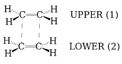
Figure 1: Two vertically-stacked ethylene molecules.

We have noticed that there seems to be a great deal of confusion in the literature regarding charge transfer in excitonic systems (e.g., see Ref. Zimmerman et al., 2009). Indeed delocalization of electron density over several molecules does not necessarily imply excitonic charge transfer; what may be taken at first as an indication of charge transfer, may turn out to be a manifestation of energy transfer. For this reason, we wish to be especially careful to define these terms within the context of excitonic theory and, in particular, we seek to explain via an algebraic example how excitations described using MOs, delocalized over several molecules in a supermolecule, may be analyzed and understood in terms of the (mainly) pairwise interaction of excitations localized on different molecules to create ET and CT excitons. In the process of this work, we shall see that single molecule spectra are shifted and single peaks may be split into multiplets when molecules form aggregates. We will call these observed multiplets Davydov multiplets and the observed splittings Davydov splittings (DSs). We emphasize that the explanation for these splittings can be different than the traditional explanation proposed by Davydov Davydov (1962) and by Kasha Kasha et al. (1965) as CT effects were not present in their models. Note, however, that including both ET and CT effects is in keeping with state-of-the-art practice in the Bethe-Salpeter equation Green’s function Cudazzo et al. (2015); Blase et al. (2018) treatment of the spectra of molecular solids Tiago et al. (2003); Cudazzo et al. (2012, 2015) though our terminology differs from theirs (their classification of an exciton as being of FR type is analogous to our classification as ET type, while we both agree in referring to CT type excitons).

In particular, we wish to show algebraically and using chemical intuition to what extent Kasha’s exciton model Kasha et al. (1965) does or does not emerge from a linear combination of singly-excited determinants over MOs. For concreteness, we will treat the $\pi$ system of vertically-stacked molecules of ethylene (Fig. 1). This is close enough to the case treated numerically in Sec. IV that we will be able to use the equations developed for vertically-stacked ethylene to help understand the exciton physics of vertically-stacked pentacenes.

II.1 Kasha’s Exciton Model

A biography highlighting key scientific achievements of Michael Kasha (1920-2013) appeared one year after his death Demchenko et al. (2014). It rightly notes that Kasha was “a key founder of modern photophysics, photochemistry, and molecular spectroscopy in condensed phases” and gives a number of examples justifying this claim Demchenko et al. (2014). Kasha’s exciton model is a venerable but still much-used model of how weak interactions between molecules lead to new features in the spectra of aggregates. It may also be applied to weakly interacting excitations between different parts of the same molecule.

Kasha’s work on excitons spans a period from 1959 to 1965 Kasha (1959, 1963); Hochstrasser and Kasha (1964); McRae and Kasha (1964); Kasha et al. (1965) with an isolated contribution in 1976 Kasha (1976). It apparently began when Albert Szent-Györgyi pointed out that some molecules phosphoresce in solid matrices but fluoresce in solution Demchenko et al. (2014). In 1963, Kasha and Robert Oppenheimer published a translation of Alexander Sergeevich Davydov’s 1951 book Theory of Molecular Excitons from the original Russian into English. Davydov had focused on the spectroscopy of molecular solids, an area for which there were very few well-resolved spectra at the time. Given the pre-computer epoch when Davydov developed his ideas, he necessarily made many simplifying approximations. Davydov’s examples focused mainly on cases where there are two molecules per unit cell, but his last chapter, entitled “Excitation Calculation of States of Molecules” included a discussion of what happens to the spectra of the biphenyl molecule when the quasi-independent excitations of the two phenyl molecules interact. This is the theory that Kasha’s group would develop as the exciton model Kasha et al. (1965) which we briefly review here.

We follow the classic 1965 paper of Kasha, Rawls, and El-Bayoumi Kasha et al. (1965) very closely, albeit with some differences in notation, and consider a van der Waals (vdW) dimer of two identical molecules which will be labeled as 1 and 2. Key approximations will be emphasized in itallics. The ground $\Psi_{1/2}^{0}$ and excited state $\Psi_{1/2}^{I}$ of the isolated molecule 1 or 2 satisfies the electronic Schrödinger equation,

$${\hat{H}}_{1/2}\Psi_{1/2}=E_{1/2}\Psi_{1/2}\,.$$ (2)

The monomer excitation energy is,

$$\omega_{1/2}^{I}=E_{1/2}^{I}-E_{1/2}^{0}\,.$$ (3)

The dimer Hamiltonian is,

$${\hat{H}}={\hat{H}}_{1}+{\hat{H}}_{2}+{\hat{V}}_{1,2}\,,$$ (4)

where ${\hat{V}}_{1,2}$ is the interaction potential. As the interaction potential is assumed small, we treat the problem perturbatively using the zero-order dimer wave function,

$$\Psi^{0}=\Psi_{1}^{0}\Psi_{2}^{0}\,.$$ (5)

The ground-state energy is then,

$$E^{0}=E_{1}^{0}+E_{2}^{0}+E^{0}_{\text{vdW}}\,,$$ (6)

where

$$E^{0}_{\text{vdW}}=\langle\Psi_{1}^{0}\Psi_{2}^{0}|{\hat{V}}_{1,2}|\Psi_{1}^{0}\Psi_{2}^{0}\rangle$$ (7)

is interpretted as the vdW energy binding the two monomers into a dimer.

The dimer excited-state wave function is assumed to be of the form,

$$\Psi^{I}=C_{1}\Psi_{1}^{I}\Psi_{2}^{0}+C_{2}\Psi_{1}^{0}\Psi_{2}^{I}\,.$$ (8)

That is, we consider that only one monomer is excited at a time and that monomer is excited to its $I$th excited state. Note that charge transfer excitations have been neglected in this exciton model. It is easy to set up the small configuration interaction problem,

$$\left[\begin{array}[]{cc}A&B\\ B&A\end{array}\right]\left(\begin{array}[]{c}C_{1}\\ C_{2}\end{array}\right)=E^{I}\left(\begin{array}[]{c}C_{1}\\ C_{2}\end{array}\right)$$ (15)

$$A=\langle\Psi_{1}^{I}\Psi_{2}^{0}|{\hat{H}}|\Psi_{1}^{I}\Psi_{2}^{0}\rangle=\langle\Psi_{1}^{0}\Psi_{2}^{I}|{\hat{H}}|\Psi_{1}^{0}\Psi_{2}^{I}\rangle$$

$$B=\langle\Psi_{1}^{I}\Psi_{2}^{0}|{\hat{H}}|\Psi_{1}^{0}\Psi_{2}^{I}\rangle=\langle\Psi_{1}^{0}\Psi_{2}^{I}|{\hat{H}}|\Psi_{1}^{I}\Psi_{2}^{0}\rangle\,,$$ (16)

whose solutions are,

$$\Psi^{I}_{\pm} = \frac{1}{\sqrt{2}}\left(\Psi_{1}^{I}\Psi_{2}^{0}\pm\Psi_{1}^{0}\Psi_{2}^{I}\right)$$

$$E^{I}_{\pm} = A\pm B\,.$$ (17)

The terms $A$ and $B$ are,

$$A=E_{1}^{I}+E_{2}^{0}+E^{I}_{\text{vdW}}$$

$$E^{I}_{\text{vdW}}=\langle\Psi_{1}^{I}\Psi_{2}^{0}|{\hat{V}}_{1,2}|\Psi_{1}^{I}\Psi_{2}^{0}\rangle$$

$$B=E_{\text{exciton splitting}}$$

$$E_{\text{exciton splitting}}=\langle\Psi_{1}^{I}\Psi_{2}^{0}|{\hat{V}}_{1,2}|\Psi_{1}^{0}\Psi_{2}^{I}\rangle$$ (18)

Hence there are two excitation energies,

$$\omega^{I}_{\pm}=\omega^{I}_{1}+\left(E^{I}_{\text{vdW}}-E^{0}_{\text{vdW}}\right)\pm E_{\text{exciton splitting}}\,.$$ (19)

The oscillator strength,

$$f_{\pm}^{I}=\frac{\omega^{I}_{\pm}}{3}|{\vec{\mu}}^{I0}_{1}\pm{\vec{\mu}}^{I0}_{2}|^{2}\,,$$ (20)

where the transition dipole moment,

$${\vec{\mu}}^{I0}_{\pm} = \langle\Psi^{I}|{\vec{r}}|\Psi_{0}\rangle$$ (21)

$$= \frac{1}{\sqrt{2}}\left(\langle\Psi_{1}^{I}\Psi_{2}^{0}|{\vec{r}}|\Psi_{1}^{0}\Psi_{2}^{0}\rangle\pm\langle\Psi_{1}^{0}\Psi_{2}^{I}|{\vec{r}}|\Psi_{1}^{0}\Psi_{2}^{0}\rangle\right)$$

$$= \frac{1}{\sqrt{2}}\left({\vec{\mu}}^{I0}_{1}\pm{\vec{\mu}}^{I0}_{2}\right)$$

Therefore each peak in the monomer absorption spectrum will be split into two exciton peaks with different intensities. Similar results emerge in the following subsections, but in a completely different way as we analyze aggregate molecular orbitals in terms of monomer molecular orbitals instead of deriving aggregate absorption spectra from monomer absorption spectra. In particular, the Davydov splitting will emerge, not as the difference between coupled excitation energies but rather as the difference between an energy-transfer (ET) excitation energy and a charge-transfer (CT) excitation energy.

The final approximation made in Kasha’s exciton model is the point dipole/point dipole approximation,

$$E_{\text{exciton splitting}}=\frac{{\vec{\mu}}^{I0}_{1}\cdot{\vec{\mu}}^{I0}_{2}}{r^{3}}-3\frac{\left({\vec{\mu}}^{I0}_{1}\cdot{\vec{r}}\right)\left({\vec{\mu}}^{I0}_{2}\cdot{\vec{r}}\right)}{r^{5}}\,.$$ (22)

This assumes molecules separated by a large distance relative to the size of the molecules. It is difficult to see how this can be applied in a quantitative fashion to the most common application of the excition model, namely to large dye molecules self-assembled into aggregates in solution, where the distance assumptions are hardly valid. In the next subsection, we derive a similar but different theory of exciton splitting which will be further justified by explicit calculations in Sec. IV. In particular, ET and CT excitation energies behave as expected for different variations on TD-DFT and on TD-DFTB.

II.2 Monomer

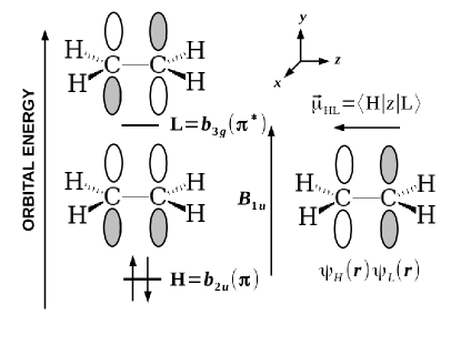
Figure 2: Ethylene highest occupied molecular orbital (H) and lowest unoccupied molecular orbital (L).

The MOs of the $\pi$ system of ethylene are shown in Fig. 2. MO symmetries have been assigned following the recommended International Union of Pure and Applied Chemistry (IUPAC) nomenclature Mulliken (1955, 1956) and the symmetry of the expected lowest energy excitations have been assigned. Of particular importance for us is the sketch of the transition density $\psi_{H}(\bf r)\psi_{L}(\bf r)$ on the right-hand side of the figure with the associated transition dipole moment $\vec{\mu}_{HL}$. Here H stands for the highest occupied molecular orbital, while L stands for the lowest unoccupied molecular orbital.

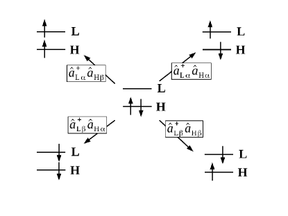
Figure 3: Two-orbital two-electron model (TOTEM).

This is evidently a two-orbital two-electron model (TOTEM, Fig. 3) and the excitations may be analyzed in this context. There are four possible one-electron excitations for the TOTEM, but spin symmetry must be taken properly into account. We shall focus on the singlet transition which goes from the ground-state determinant $\Phi$ to the state,

$${}^{1}(H,L)=\frac{1}{\sqrt{2}}\left({\hat{a}}_{L\alpha}^{\dagger}{\hat{a}}_{H\alpha}+{\hat{a}}_{L\beta}^{\dagger}{\hat{a}}_{H\beta}\right)\Phi\,,$$ (23)

where $\alpha$ and $\beta$ refer to spin states (i.e., spin up and spin down, respectively) and ${\hat{a}}_{L\alpha/\beta}^{\dagger}{\hat{a}}_{H\alpha\beta}$ is an operator in second quantization formalism meaning to remove one electron from $H\alpha/\beta$ and place it into $L\alpha/\beta$. In the specific case of the TOTEM, we may just write

$${}^{1}(H,L) = \frac{1}{\sqrt{2}}\left(|H,{\bar{L}}|+|L,{\bar{H}}|\right)$$ (24)

$$= \left[\frac{1}{\sqrt{2}}\left(H(1)L(2)+L(1)H(2)\right)\right]$$

$$\times \left[\frac{1}{\sqrt{2}}\left(\alpha(1)\beta(2)-\beta(1)\alpha(2)\right)\right]\,.$$

There are also three triplet states which are degenerate in the absence of spin-orbit coupling,

$${}^{3}(H,L)_{M_{S}=+1} = |H,L|$$

$$= \left[\frac{1}{\sqrt{2}}\left(H(1)L(2)-L(1)H(2)\right)\right]$$

$$\times \left[\alpha(1)\alpha(2)\right]$$

$${}^{3}(H,L)_{M_{S}=0} = \frac{1}{\sqrt{2}}\left(|H,\bar{L}|-|L,\bar{H}|\right)$$

$$= \left[\frac{1}{\sqrt{2}}\left(H(1)L(2)-L(1)H(2)\right)\right]$$

$$\times \left[\frac{1}{\sqrt{2}}\left(\alpha(1)\beta(2)+\beta(1)\alpha(2)\right)\right]$$

$${}^{3}(H,L)_{M_{S}=-1} = |\bar{H},\bar{L}|$$ (25)

$$= \left[\frac{1}{\sqrt{2}}\left(H(1)L(2)-L(1)H(2)\right)\right]$$

$$\times \left[\beta(1)\beta(2)\right]\,,$$

which will not concern us here.

II.3 Dimer

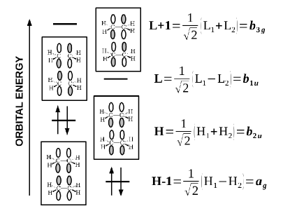
Figure 4: MO diagram for two stacked ethylene molecules. White indicates the positive phase parts of the $p$ functions while grey indicates the negative phase parts. Overlap between the MOs on different molecules have been neglected in normalizing the supermolecule MOs.

We are now ready to treat two interacting stacked ethylene molecules. This system has been studied previously in the context of excitonic effects Koutecký and Paldus (1963); Scholes and Ghiggino (1994); Harcourt et al. (1994); Scholes et al. (1995) and at a greater level of sophistication than that needed here. Instead, we try to keep our analysis as simple as possible by assuming weak interactions between the molecules so that we may go to trimers and oligomers. Thus the analysis in the present section is most correct only at large intermolecular distances.

The corresponding dimer MO diagram (Fig. 4) under the assumption of weak interactions between the molecules. Here, after ordering MOs by energy, H$-n$ is the $n$th occupied MO below H and L$+n$ is the $n$th unoccupied MO above L. As expected the number of nodal planes also increases with MO energy. Although we might think of this as a four-orbital four-electron model, we would like to think in terms of the exciton model, which we shall refer to as (TOTEM)² for evident reasons. Both energy transfer (ET) and charge transfer (CT) excitons will emerge from our analysis.

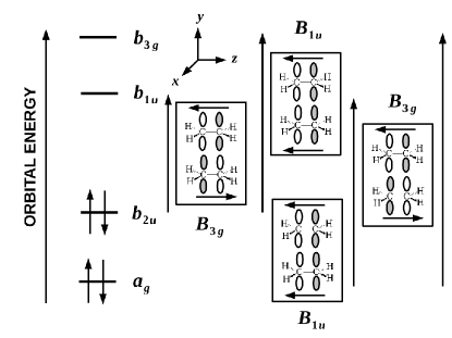
Figure 5: The four transitions in (TOTEM)² and their associated transition dipole moments.

Figure 5 shows the four possible singlet transitions in (TOTEM)² from the point of view of the MOs of the supermolecule composed of the two weakly-interacting ethylene molecules. Exciton analysis means that we want to re-express the description of the excitations so that they are no longer expressed in terms of the MOs of the supermolecule but rather are expressed in terms of ET and CT excitons involving the MOs (H₁ and L₁) of molecule 1 and the MOs (H₂ and L₂) of molecule 2. Figure 5 shows that the transitions divide neatly into two symmetry types, namely $B_{1u}$ and $B_{3g}$. This simplifies our analysis as only orbitals of the same symmetry may mix.

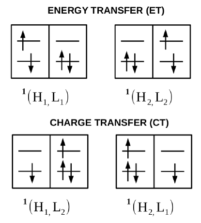
Figure 6: Exciton model classification of transitions in the (TOTEM)² model. In each double box, the left hand side shows the orbital occupancy of the MOs in molecule 1 while the right hand side shows the orbital occupancy of the MOs in molecule 2.

Physically re-expressing supermolecule excitations in terms of ET and CT excitons on individual molecules can only happen when there are enough degrees of liberty — and, in particular, quasidegenerate states — that delocalized orbitals can be re-expressed in terms of more localized orbitals. This does not happen for the $B_{3g}$ transitions. In fact, the first $B_{3g}$ transition is expected to be heavily dominated by the ${}^{1}(H,L)$ configuration and the remaining $B_{3g}$ transition should be dominated by the ${}^{1}(H-1,L+1)$ configuration. However the $B_{3g}$ transitions are spectroscopically dark. So we will just go directly on to the $B_{1u}$ orbitals.

The most general $B_{1u}$ transition is of the form,

$$\Psi=c_{1}\,^{1}(H,L+1)+c_{2}\,^{1}(H-1,L)\,.$$ (26)

Expressing the aggregate MOs in terms of the local MOs of molecules 1 and 2 as given in Fig. 4 leads to,

$$\Psi=\frac{c_{1}+c_{2}}{\sqrt{2}}\mbox{ET}_{12}+\frac{c_{1}-c_{2}}{\sqrt{2}}\mbox{CT}_{12}\,,$$ (27)

where,

$$\mbox{ET}_{12}=\frac{1}{\sqrt{2}}\left[{}^{1}(H_{1},L_{1})+^{1}(H_{2},L_{2})\right]$$ (28)

is the pairwise ET exciton and,

$$\mbox{CT}_{12}=\frac{1}{\sqrt{2}}\left[{}^{1}(H_{1},L_{2})+^{1}(H_{2},L_{1})\right]$$ (29)

is the corresponding CT exciton. (See Fig. 6. Note that we make no attempt to distinguish between Förster and Dexter ET excitons.) Physically we expect the ${}^{1}(H-1,L)$ and ${}^{1}(H,L+1)$ transitions to be quasidegenerate (i.e., $c_{1}\approx c_{2}$) as often happens in organic molecules with a conjugated $\pi$ system. Kasha’s theory is recovered for exact degeneracy (i.e., when $c_{1}=\pm c_{2}=1/\sqrt{2}$). More specifically, we would get a single ET peak corresponding to the bright state in Kasha’s theory, but we do not see the dark ET peak in our analysis because it has $B_{3g}$ symmetry. Note however that the $B_{1u}$ CT peak is likely to be less bright in practice than the ET peak so that we will see something like the situation shown in Fig. 7. We refer to the difference of the ET and CT states as the Davydov splitting (DS = ET - CT).

An important aspect of applications of Kasha’s theory is that it can tell us something about the mutual orientation of molecules. Thus Kasha’s theory may be further developed to show a red shift upon the formation of head-to-tail dimers when the CT state is bright and the ET state is dark Kasha et al. (1965). Other configurations yield two peaks with an experimentally observable DS whose relative intensities may be analyzed to give information about the relative orientation of the molecules in the dimer Kasha et al. (1965). It will be of interest once we have identified the true nature of the exciton peaks to apply Kasha’s naïve theory as if only ET excitonic effects were present because this remains a common way to analyze some experiments. We will return to this point at the end of Sec. IV by applying Kasha’s naïve theory to our calculated TD-DFT and TD-DFTB spectra.

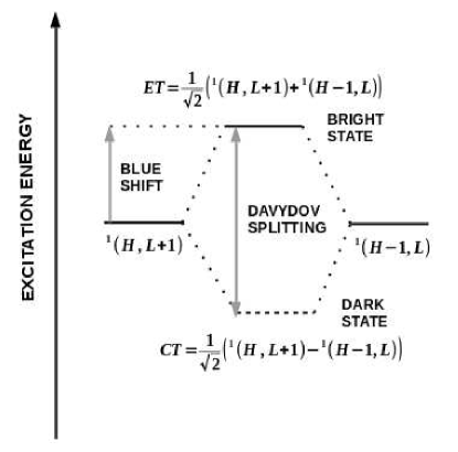
Figure 7: Schematic of the present theory for two parallel stacked molecules.

II.4 Trimer

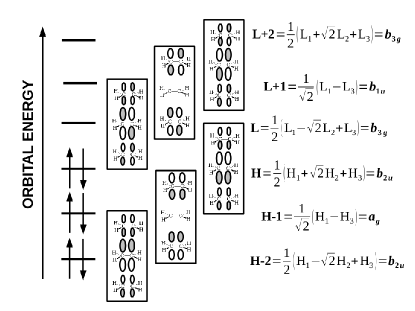
Figure 8: MO diagram for three stacked ethylene molecules. White indicates the positive phase parts of the $p$ functions while grey indicates the negative phase parts. Overlap between the MOs on different molecules have been neglected in normalizing the supermolecule MOs.

Three stacked trimers introduce another key level of complexity in the exciton model. We now have an interior molecule interacting with two outer molecules. This asymmetry means that transitions forbidden, and hence dark, in the dimer may now be allowed, and hence bright, in the trimer. Figure 8 shows the (TOTEM)³ MOs deduced by analogy with the simple Hückel solution for the propenyl radical.

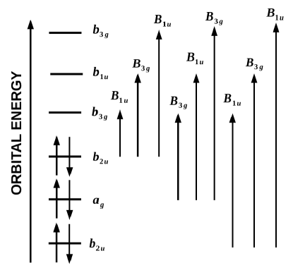
Figure 9: The nine single excitations for three stacked ethylene molecules along with their symmetry assignments.

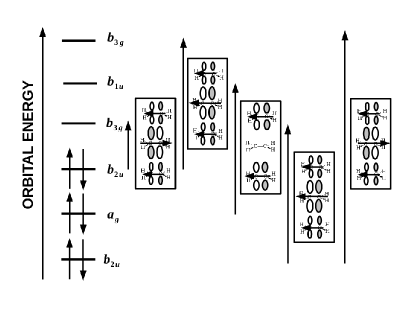
Figure 10: The transition densities for the five symmetry allowed $B_{1u}$ singlet excitations.

Figure 9 show the nine single excitations. Only the five $B_{1u}$ transitions are symmetry allowed for absorption spectroscopy. Figure 10 shows the transition densities for the five symmetry-allowed singlet transitions. We thus restrict our analysis to the linear combination of only these states,

$$\Psi = c_{1}\,^{1}(H,L)+c_{2}\,^{1}(H,L+2)+c_{3}\,^{1}(H-1,L+1)$$ (30)

$$+ c_{4}\,^{1}(H-2,L)+c_{5}\,^{1}(H-2,L+2)\,.$$

Furthermore, we will use chemical intuition to predict the general form of these five allowed transitions. In particular, only the ${}^{1}(H,L+2)$, ${}^{1}(H-1,H+1)$, and ${}^{1}(H-2,L)$ states are expected to be degenerate enough to mix to form pairwise ET and CT excitons. This gives, after some algebra,

$$\Psi = c_{1}\,^{1}(H,L)$$ (31)

$$+ \frac{3c_{2}+2c_{3}+3c_{4}}{2\sqrt{6}}\left(\frac{\mbox{ET}_{12}+\mbox{ET}_{23}}{\sqrt{3}}\right)$$

$$+ \sqrt{\frac{2}{3}}c_{3}\left\{\frac{\sqrt{3}}{2}\left[\mbox{ET}_{13}-\frac{1}{3}\left(\mbox{ET}_{12}+\mbox{ET}_{23}\right)\right]\right\}$$

$$+ \frac{c_{2}-c_{4}}{\sqrt{2}}\left(\frac{\mbox{CT}_{12}+\mbox{CT}_{23}}{\sqrt{2}}\right)$$

$$+ \frac{c_{2}-2c_{3}+c_{4}}{2\sqrt{2}}\mbox{CT}_{13}$$

$$+ c_{5}\,^{1}(H-2,L+2)\,,$$

where the notation is an obvious generalization of that given in Eqs. (28) and (29) and where the states have been orthonormalized. To a first approximation, the ${}^{1}(H,L)$ is too low in energy to mix with the other terms and ${}^{1}(H-2,L+2)$ is too high in energy to mix with the other terms. The ET and CT excitons lie in-between these in energy. Notice, however, that the CT terms vanish if $c_{3}=c_{4}=c_{5}$ which is expected to be often approximately the case. Note also that the pairwise ET terms are not orthogonal to each other as, for example, $\langle\mbox{ET}_{12}|\mbox{ET}_{23}\rangle=\langle\,^{1}(H_{2},L_{2})|\,^{1}(H_{2},L_{2})\rangle/2=1/2$. However the ET terms have been grouped to reflect the symmetry of the stack and the distance over which energy must be transfered.

As we shall see numerically in Sec. IV for the trimer of stacked pentacene molecules, each term is a reasonably good first approximation to a calculated TD-DFT excitation. Notice how the present model differs from Kasha’s orginal model: (i) supermolecule MO excitations, such as ${}^{1}(H,L)$, which are better described in terms of supermolecule MOs than in terms of local MOs and (ii) CT excitons are only expected to cancel approximately in practical calculations. In reality ET and CT terms should mix.

The stacked trimer represents the simplest model where one molecule is interacting with two surrounding molecules. As such, it captures the basic physics of exciton interactions between neighboring molecules ($1\leftrightarrow 2$ and $2\leftrightarrow 3$). Equation (31) shows that neglect of $1\leftrightarrow 3$ interactions (i.e., CT₁₃ and ET₁₃ and their required orthogonalization to the other terms) leads to only a single Davydov splitting into one ET and one CT peak. However a more careful analysis should include $1\leftrightarrow 3$ interactions and Davydov multiplets may also be expected to be observed.

II.5 Higher Oligomers

The extension of these ideas to (TOTEM)^N for $N>2$ is in principle straightforward but becomes increasingly complicated. However, it does not seem unreasonable to expect the structure of the spectrum to stabilize after a few layers, because the dominant interactions are expected to be primarily only between adjacent molecules. Thus we may anticipate that the numerical results in Sec. IV should already show most of the qualitatively important features when $N=3$ that are seen for still larger values of $N$.

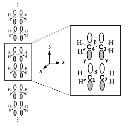
Figure 11: Periodic model labeling and hopping parameters used for our stacked ethylene tight-binding calculation.

We may explore this further by a back of the envelope tight-binding calculation for the periodic system of stacked ethylenes shown in Fig. 11. This is basically just a periodic simple Hückel calculation and so should be largely familiar to Quantum Chemists, even if the precise language and periodic symmetry adapted linear combinations may take a little getting used to.

To carry out our tight-binding calculation, we must include two ethylene molecules in the unit cell. In the exciton model, the MOs of each ethylene molecule $\chi_{\mu}(\vec{r})$ are looked on much like local AOs (LAOs). Combining them gives us a set of (TOTEM)² MOs which become local MOs (LMOs)

$$\psi_{i}(\vec{r})=\sum_{\mu}\chi_{\mu}({\vec{r}})c_{\mu,i}\,.$$ (32)

Periodic symmetry-adapted linear combinations have the form of crystal MOs (CMOs)

$$\psi_{i}(\vec{r};\vec{k})=\sum_{\vec{R}}\psi_{i}(\vec{r}-\vec{R})e^{i\vec{k}\cdot\vec{R}}\,,$$ (33)

which may also be written as,

$$\psi_{i}({\vec{r}};{\vec{k}})=\sum_{\mu}\chi_{\mu}({\vec{r}};\vec{k})c_{\mu,i}({\vec{k}})\,,$$ (34)

in terms of crystal AOs (CAOs),

$$\chi_{\mu}({\vec{r}};{\vec{k}})=\frac{1}{\sqrt{N}}\chi_{\mu}({\vec{r}}-{\vec{R}})e^{i{\vec{k}}\cdot{\vec{R}}}\,.$$ (35)

The factor $N$ in this formalism represents the number of atoms in a fictitious “finite crystal.” It has been introduced for convenience, but it not really necessary. The wave vector ${\vec{k}}$ serves both as a symmetry label and may also be viewed as a sort of electron momentum which can be used in selection rules. The $\vec{k}$-block of the CMO matrix equation is

$${\bf h}({\vec{k}})\vec{c}_{i}({\vec{k}})=\epsilon_{i}({\vec{k}}){\bf s}({\vec{k}})\vec{c}_{i}({\vec{k}})\,,$$ (36)

where the matrix elements of the overlap matrix are given by,

$$s_{\mu,\nu}({\vec{k}}) = \sum_{\vec{R}}s^{({\vec{R}})}_{\mu,\nu}e^{i{\vec{k}}\cdot{\vec{R}}}$$

$$s^{({\vec{R}})}_{\mu,\nu} = \int_{V=N\Omega}\chi^{*}_{\mu}({\vec{r}}+{\vec{R}})\chi_{\nu}({\vec{r}})\,d{\vec{r}}\,,$$ (37)

and the matrix elements of the hamiltonian matrix are given by,

$$h_{\mu,\nu}({\vec{k}}) = \sum_{\vec{R}}h^{({\vec{R}})}_{\mu,\nu}e^{i{\vec{k}}\cdot{\vec{R}}}$$

$$h^{({\vec{R}})}_{\mu,\nu} = \int_{V=N\Omega}\chi^{*}_{\mu}({\vec{r}}+{\vec{R}})\hat{h}\chi_{\nu}({\vec{r}})\,d{\vec{r}}\,.$$ (38)

Here $\Omega$ is the volume of the unit cell and $N\Omega$ is the volume of the fictitious “finite crystal.”

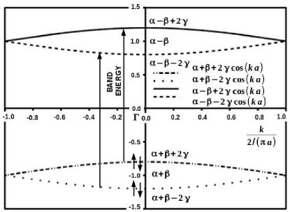
Figure 12: Bands for the stacked ethylene tight-binding model with $\alpha=0$, $\beta=-1$, and $\gamma=0.1$. The paired arrows ($\uparrow\downarrow$) are meant to indicate filled bands below the fermi level.

Our model is subject to several simplifications. For one, the wave vector is a number $k$ since our system is periodic in a single dimension ($y$). We will follow the common practice of assuming that the overlap matrix ${\bf s}(k)$ is the identity. The hamiltonian matrix ${\bf h}(k)$ is then constructed from the on-sight (i.e., coulomb) integral $\alpha$ and the hopping (i.e., resonance) integrals $\beta$ between the $p$ orbitals within each ethylenes and $\gamma$ between adjacent $p$ orbitals in different ethylene molecules. Note that $\alpha,\beta<0$ but that $\gamma>0$ for this particular configuration. The position vector ${\vec{R}}$ is $Y$ so that

$${\bf h}(k)=\sum_{Y}{\bf h}^{(Y)}e^{ikY}\,.$$ (39)

where,

$${\bf h}^{(Y)} = \left[\begin{array}[]{cc}{\bf A}&{\bf B}\\ {\bf C}&{\bf A}\end{array}\right]$$ (42)

$${\bf A} = \left[\begin{array}[]{cc}\alpha\delta_{Y,0}&\beta\delta_{Y,0}\\ \beta\delta_{Y,0}&\alpha\delta_{Y,0}\end{array}\right]$$ (45)

$${\bf B} = \left[\begin{array}[]{cc}0&\gamma\left(\delta_{Y,0}+\delta_{Y,+a}\right)\\ \gamma\left(\delta_{Y,0}+\delta_{Y,+a}\right)&0\end{array}\right]$$ (48)

$${\bf C} = \left[\begin{array}[]{cc}0&\gamma\left(\delta_{Y,0}+\delta_{Y,-a}\right)\\ \gamma\left(\delta_{Y,0}+\delta_{Y,-a}\right)&0\end{array}\right]\,,$$ (51)

and $a$ is the $y$-distance between ethylene molecules as opposed to the unit cell parameter which is equal to $2a$. Applying Eq. (39) to Eq. (51) then gives that

$${\bf h}(k) = \left[\begin{array}[]{cc}{\bf A}&{\bf B}(k)\\ {\bf C}(k)&{\bf A}\end{array}\right]$$ (54)

$${\bf A} = \left[\begin{array}[]{cc}\alpha&\beta\\ \beta&\alpha\end{array}\right]$$ (57)

$${\bf B}(k) = \left[\begin{array}[]{cc}0&\gamma\left(1+e^{i2ka}\right)\\ \gamma\left(1+e^{i2ka}\right)&0\end{array}\right]$$ (60)

$${\bf C}(k) = \left[\begin{array}[]{cc}0&\gamma\left(1+e^{-i2ka}\right)\\ \gamma\left(1+e^{-i2ka}\right)&0\end{array}\right]\,.$$ (63)

This has four solutions, namely:

$$\epsilon_{1}(k)=\alpha+\beta+2\gamma\cos(ka) \leftrightarrow \vec{c}_{1}(k)=\left(\begin{array}[]{c}1\\ 1\\ +z^{*}/|z|\\ +z^{*}|z|\end{array}\right)$$ (68)

$$\epsilon_{2}(k)=\alpha+\beta-2\gamma\cos(ka) \leftrightarrow \vec{c}_{2}(k)=\left(\begin{array}[]{c}1\\ 1\\ -z^{*}/|z|\\ -z^{*}//|z|\end{array}\right)$$ (73)

$$\epsilon_{3}(k)=\alpha-\beta-2\gamma\cos(ka) \leftrightarrow \vec{c}_{3}(k)=\left(\begin{array}[]{c}1\\ -1\\ +z^{*}/|z|\\ -z^{*}/|z|\end{array}\right)$$ (78)

$$\epsilon_{4}(k)=\alpha-\beta+2\gamma\cos(ka) \leftrightarrow \vec{c}_{4}(k)=\left(\begin{array}[]{c}1\\ -1\\ -z^{*}/|z|\\ +z^{*}/|z|\end{array}\right)\,,$$ (83)

where,

$$z=1+e^{i2ka}\,.$$ (85)

The associated band diagram is shown in Fig. 12. This is a direct band system. Assuming the $\Gamma$ point and no momentum transfer to the lattice, then the two allowed transitions are those shown by vertical arrows. The corresponding CMOs (Fig. 13) bear a close resemblence to the MOs of the (TOTEM)² dimer (Fig. 5), showing that the (TOTEM)² analysis also applies in the periodic (TOTEM)^N case.

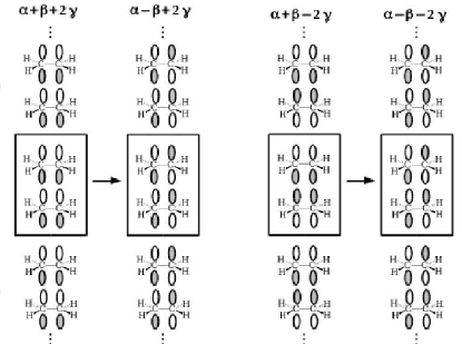
Figure 13: The CMOs for the optically-allowed transitions of (TOTEM)^N at the $\Gamma$-point.

Finally, it is illuminating to apply the same tight-binding model to the (TOTEM)² dimer. The hamiltonian matrix to be diagonalized is then,

$${\bf h}(k) = \left[\begin{array}[]{cc}{\bf A}&{\bf B}\\ {\bf B}&{\bf A}\end{array}\right]$$ (88)

$${\bf A} = \left[\begin{array}[]{cc}\alpha&\beta\\ \beta&\alpha\end{array}\right]$$ (91)

$${\bf B} = \left[\begin{array}[]{cc}0&\gamma\\ \gamma&0\end{array}\right]\,,$$ (94)

which has the four solutions,

$$\epsilon_{1}=\alpha+\beta+\gamma \leftrightarrow \vec{c}_{1}=\left(\begin{array}[]{c}1\\ 1\\ 1\\ 1\end{array}\right)$$ (99)

$$\epsilon_{2}=\alpha+\beta-\gamma \leftrightarrow \vec{c}_{2}=\left(\begin{array}[]{c}1\\ 1\\ -1\\ -1\end{array}\right)$$ (104)

$$\epsilon_{3}=\alpha-\beta-\gamma \leftrightarrow \vec{c}_{3}=\left(\begin{array}[]{c}1\\ -1\\ 1\\ -1\end{array}\right)$$ (109)

$$\epsilon_{4}(k)=\alpha-\beta+\gamma \leftrightarrow \vec{c}_{4}=\left(\begin{array}[]{c}1\\ -1\\ -1\\ 1\end{array}\right)\,.$$ (114)

Comparing with the band solution for the periodic system (TOTEM)^N, we see that the energy levels are displaced by $\gamma$ in (TOTEM)² rather than by $2\gamma$ in (TOTEM)^N, because each ethylene in (TOTEM)² is only in contact with a single other ethylene, while each ethylene in (TOTEM)^N is in contact with two other ethylene molecules. However the key energy differences are the same for (TOTEM)² and (TOTEM)^N, lending reassurance that the fundamental analysis of the dimer model also applies for larger parallel stacks of ethylene molecules. On the other hand, inclusion of nonnearest neighbor interactions in the model is expected to yield small contributions from higher-order Davydov multiplets, even if our simple model captures the main qualitative aspects of ET and CT excitons in the stack of molecules.

This completes our analytic study of stacked ethylene dimers. In the Sec. IV, we will apply this analysis to stacked pentamers and use it to gain a deeper insight into how different variations of TD-DFT and TD-DFTB work.

III Computational Details

Two programs were used to carry out the calculations reported in this paper, namely Gaussian09 Frisch et al. for DFT (Appendix A) and TD-DFT (Appendix B) calculations and DFTBaby Humeniuk and Mitrić (2015); Humeniuk and Mitrič (2017) for DFTB (Appendix C) and TD-DFTB (Appendix D) calculations. Note that, although Gaussian09 does have the ability to carry out DFTB calculations, only DFTBaby allows us to carry out state-of-the-art TD-lc-DFTB calculations. We will first describe the options used with each program in more detail. We will then go on to describe how the programs were used in structural and spectral studies.

Gaussian09 Frisch et al. calculations may be described in terms of a “theoretical model” (p. 5, Ref. Hehre et al., 1986) which is fully specified, in our case, by indicating for an excited-state (i.e., TD) calculation, the the choice of functional and the orbital basis set. This is conveniently expressed in expanded notation as

(TD-)DFA1/Basis1//DFA2/Basis2

(p. 96, Ref. Hehre et al., 1986), where DFA2 is the density-functional approximation used for the geometry optimzation and Basis2 is the corresponding basis set used for the geometry optimization, and DFA1 is the density-functional approximation used used for the TD-DFT calculation and Basis1 is the corresponding orbital basis used in the TD-DFT calculation. The density-functionals used (LDA, B3LYP, HF, CAM-B3LYP with or without Grimme’s D3 correction) are described in Appendix A. Two orbital basis sets were used here, namely the minimal STO-3G basis set Hehre et al. (1969, 1970) and the much more flexible 6-31G(d,p) split-valence (hydrogen Ditchfield et al. (1971), carbon Hehre et al. (1972)) plus polarization basis set Harihan and Pople (1972). An example of the expanded notation is that TD-CAM-B3LYP/6-31G(d,p)//D3-CAM-B3LYP/6-31G(d,p) means that the geometry of the molecule was optimized using the 6-31G(d,p) basis set using the CAM-B3LYP functional with the D3 dispersion correction. Then a TD-DFT calculation was carried out at that geometry using the 6-31G(d,p) orbital basis set and the CAM-B3LYP functional (Appendix B). Often we will use a shorter nomenclature when the details of the theoretical model are clear from context.

DFTBaby Humeniuk and Mitrić (2015); Humeniuk and Mitrič (2017) was used to carry out lc-DFTB (Appendix C) and TD-lc-DFTB (Appendix D) calculations. The values for the confinement radius $r_{0}$ and the Hubbard parameter $U_{H}$ that were used to parameterize the electronic part of DFTB are shown in Table I of Ref. Humeniuk and Mitrić, 2015. The parameter for the lc correction was set to $R_{\text{lc}}$ = 3.03 bohr so $\mu=1/R_{\text{lc}}=0.33\,\,\mbox{bohr${}^{-1}$}$, which is a reasonable compromise between $\mu=0.33\,\,\mbox{bohr${}^{-1}$}$ used in the CAM-B3LYP functional and $\mu=0.4\,\,\mbox{bohr${}^{-1}$}$ used in the LRC family of functionals.

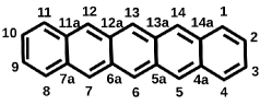
Figure 14: Pentacene carbon numbering.

Our structural calculations started with initial x-ray crystallography geometries taken from the Crystallography Open Database (COD) Dorset and McCourt (1994); Schiefer et al. (2007). We will use the standard numbering of pentacene carbon shown in Fig. 14. We first optimized the monomer geometry and calculated its absorption spectrum at each level. Vibrational frequencies were calculated to make sure that the optimized structures were true minima. We then went on to study an ideal parallel stacked model in which B3LYP/6-31G(d,p) optimized monomers were $\pi$-stacked vertically face-to-face with a fixed distance $R$ between them (Fig. 15). The distance $R$ was optimized for the tetramer using different methods and then this distance was used in studying stacks of different sizes. Finally we studied calculated absorption spectra for cluster models cut out of the experimental herringbone structure without any geometry optimization.

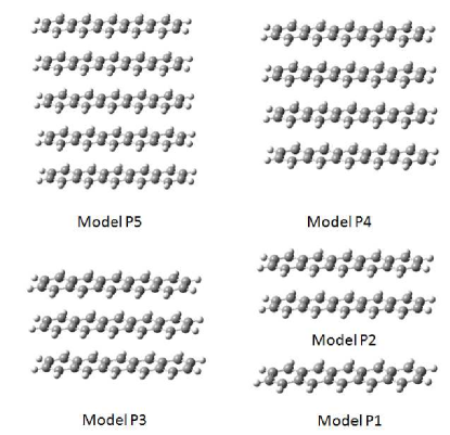
Figure 15: The configurations of the five models of parallel stacked pentacene (P$n$ stands for $n$ parallel stacked pentacenes).

IV Results

Our goal in this section is to evaluate state-of-the-art (TD-)DFTB calculations of excitons in pentacene aggregates with state-of-the-art (TD-)DFT calculations on the same systems. We would also like to get a feeling for the relative importance of ET versus CT excitons. This involves three levels of calculation on three classes of systems. The three levels of calculation are first high-quality (TD-)DFT/6-31G(d,p) calculations aimed at obtaining good quality reference calculations which can be compared to experiment as a reality check. The second type of calculation consists of minimum basis set
(TD-)DFT/STO-3G calculations as our ultimate goal is to evaluate the third method, namely the minimal basis set semi-empirical (TD-)DFTB method. The systems considered are first an isolated gas-phase pentacene molecule, second a series of parallel-stacked pentacene molecules as these parallel the theory already presented in Sec. II, and lastly a subunit of the known structure of crystalline pentacene.

IV.1 Monomer

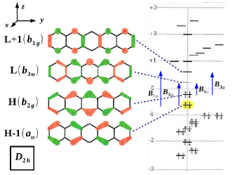
Figure 16: Simple Hückel molecular orbital theory results for the pentacene monomer.

Although our primary interest here is in the absorption spectrum of the monomer, it is useful to begin with a review of the molecular orbitals (MOs). Figure 16 shows the result of a simple Hückel MO calculation with the SHMO calculator Rauk (accessed 22 July 2016). MO symmetries have been assigned following the recommended IUPAC nomenclature Mulliken (1955, 1956) and the symmetry of the expected lowest energy excitations have been assigned.

The monomer geometry has been optimized at the LDA/STO-3G, LDA/6-31G(d,p), B3LYP/STO-3G, B3LYP/6-31G(d,p), CAM-B3LYP/STO-3G, CAM-B3LYP/6-31G(d,p), DFTB, and lc-DFTB levels of theory. The orbitals at the resultant optimized gometries have been visualized (e.g., Fig. 17) and are found to be qualitatively similar to those obtained from simple Hückel MO theory. This is important as it is then relatively easy to make a connection between the results of stacked pentacene molecules and the theoretical discussion of Sec. II for stacked ethylene molecules.

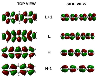
Figure 17: Pentacene monomer B3LYP/6-31G(d,p) MOs.

a)
b)
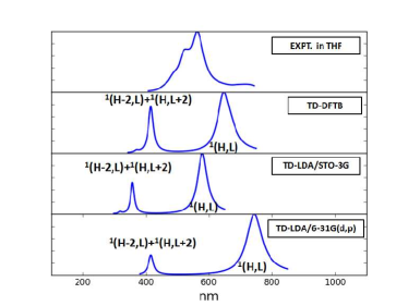
c)

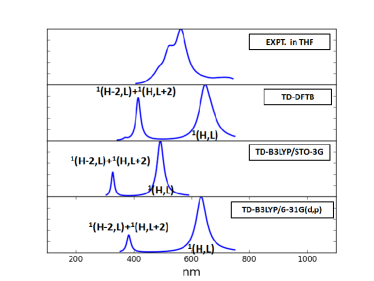
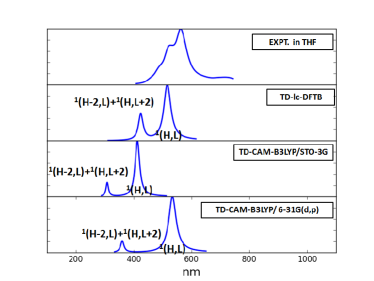
Figure 18: Pentacene monomer absorption spectra: (a) TD-LDA, TD-DFTB, and experiment; (b) TD-B3LYP, TD-DFTB, and experiment; (c) TD-CAM-B3LYP, TD-lc-DFTB, and experiment. The experimental curve is a spectrum measured in tetrahydrofuran. Intensities are in arbitrary units.

Figure 18 compares the calculated monomer absorption spectra with the experimental spectrum measured in tetrahydrofuran (data obtained by plot digitization Huwaldt (accessed 28 June 2017) of Fig. 1 of Ref. Maliakal et al., 2004). Note that TD-DFT and TD-DFTB (and TD-lc-DFTB) calculations give qualitatively similar spectra in terms of the number and spacing of peaks, though not all peaks are shown in Fig. 18. Our concern is primarily with the lowest energy (i.e., longest wavelength) transitions.

Let us first look at the TD-DFT calculations with the 6-31G(d,p) basis set using different functionals. The TD-LDA/6-31G(d,p) spectrum is red-shifted with respect to the experimental spectrum. The TD-B3LYP/6-31G(d,p) spectrum, which includes some HF exchange via a global hybrid, brings us closer to the experimental spectrum. Finally the TD-CAM-B3LYP/6-31G(d,p) spectrum, which includes even more HF exchange to decribe the long-range part of the electron-electron repulsion, matches the experimental spectrum very well. Of course, this should be taken with a certain amount of scepticism because the experimental spectrum is measured in solution while the theoretical calculations are for the gas phase and neglect any vibrational contributions.

Let us now turn to the TD-DFTB and TD-lc-DFTB calculations. Since these are semi-empirical calculations, they are expected to be similar to TD-DFT/STO-3G calculations in that DFTB calculations are parameterized assuming a minimal basis set. This might be expected to show up in the number of underlying degrees of freedom and hence in the complexity of the calculated absorption spectra. Indeed this does seem to be the case in that the longest wavelength TD-CAM-B3YLP/6-31G(d,p) peak shows more complexity than does the longest wavelength TD-lc-DFTB or TD-DFTB peak. (This difference is not visible in Fig. 18, but rather in the underlying stick spectra.) However the TD-lc-DFTB and TD-DFTB spectra are red-shifted compared to the correspondingly TD-DFT/STO-3G spectra. This brings the TD-DFTB spectrum in remarkably good correspondance with the TD-B3LYP/6-31G(d,p) spectrum and the TD-lc-DFTB spectrum in remarkably good correspondance with the TD-CAM-B3LYP/6-31G(d,p) spectrum.

Table 1: Monomer lowest energy peak ¹(H,L) calculated with various methods.

Method
State	$f$ (unitless)	$\lambda$ (nm)	$\Delta E$ (eV)
TD-LDA/6-31G(d,p)//LDA/6-31G(d,p)
$1\,^{1}B_{1u}$	0.0234	744	1.67
TD-LDA/STO-3G//LDA/STO-3G
$1\,^{1}B_{1u}$	0.0325	579	2.14
TD-B3LYP/6-31G(d,p)//B3LYP/6-31G(d,p)
$1\,^{1}B_{1u}$	0.0415	633	1.96
TD-B3LYP/STO-3G//B3LYP/STO-3G
$1\,^{1}B_{1u}$	0.0596	492	2.52
TD-DFTB//DFTB
$1\,^{1}B_{1u}$	0.1594	646	1.92
TD-CAM-B3LYP/6-31G(d,p)//B3LYP/6-31G(d,p)
$1\,^{1}B_{1u}$	0.0750	534	2.32
TD-CAM-B3LYP/STO-3G//CAM-B3LYP/STO-3G
$1\,^{1}B_{1u}$	0.1070	412	3.01
TD-lc-DFTB//lc-DFTB
$1\,^{1}B_{1u}$	0.3212	515	2.40
HF/6-31G(d,p)//B3LYP/6-31G(d,p)
$1\,^{1}B_{1u}$	0.1436	491	2.53
HF/STO-3G//B3LYP/6-31G(d,p)
$1\,^{1}B_{1u}$	0.2279	357	3.47

Some rough assignments are given, based upon MO contributions to the TD-DFT and TD-DFTB (or TD-lc-DFTB) coefficients. The lowest energy peaks (Table 1) are singlet HOMO $\rightarrow$ LUMO transitions [¹(H,L)]. The ¹(H,L) TD-CAM-B3YLP/6-31G(d,p) peak is at 534 nm, which may be compared with the corresponding experimental value of about 540 nm from gas phase spectroscopy Heinecke et al. (1998) and spectroscopy of isolated pentacene molecules in rare gas matrices Halasinski et al. (2000). The next lowest energy peaks have mixed ¹(H-2,L) and ¹(H,L+2) character as we have mentioned (Sec. II) often occurs in the excitation spectra of $\pi$-conjugated molecules.

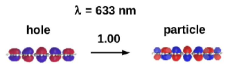
Figure 19: Monomer NTOs and renormalized coefficient: TD-B3LYP/6-31G(d,p)//B3LYP/6-31G(d,p) 633 nm.

It is especially important to confirm our ${}^{1}(H,L)$ peak assignment. Figure 19 shows the natural transition orbitals (NTOs) associated with the lower energy peak in the spectrum. Comparison with the nodal structure in Figs. 16 and 17 confirms that this is indeed the ${}^{1}(H,L)$ transition.

Notice that there is a close analogy between the TOTEM model in ethylene and that of pentacene. In particular, the part of the H and L MOs on carbons 6 and 13 in pentacene (see Fig. 14) corresponds to a $\pi^{*}\rightarrow\pi$. This is sufficiently analogous to the $\pi\rightarrow\pi^{*}$ transition in ethylene that essentially the same theoretical analysis goes through for pentacene as for ethylene and we will make great use of this observation in the next subsection.

IV.2 Stacking

We are concerned with the model of equally-spaced stacked pentacenes shown in Fig. 15. This model, though far from the observed herringbone structure of solid pentacene, is interesting because of its obvious analogy to graphite and because it may be readily compared with the model of equally-spaced stacked ethylenes discussed in the previous section.

IV.2.1 Intermolecular forces

Equally-spaced parallel stacked pentacenes were prepared by optimizing the intermolecular distance for stacked tetramers without reoptimizing the individual molecules. The tetramer stacked structure is expected to be bound together by van der Waals forces at a distance similar to that in graphene, namely about 3 Å Alam et al. (2011).

a)
b)
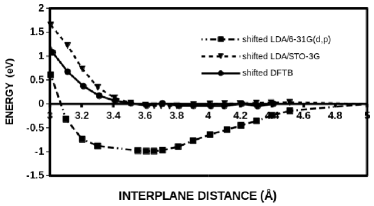
c)

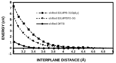
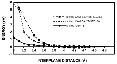
Figure 20: Pentacene tetramer potential energy surfaces without dispersion correction: (a) LDA and DFTB; (b) B3LYP and DFTB; (c) CAM-B3LYP, lc-DFTB.

Figure 20 shows the resultant PES for molecules without dispersion correction. As a general rule, DFT can only describe forces between atoms in regions of space where the electron density is significant. Uncorrected DFT is usually unable to describe van der Waals binding as such binding takes place at intermolecular distances where the molecular densities do not overlap significantly. As seen in Fig. 20, LDA/6-31G(d,p) shows an accidental minimum at about 3.65 Å but LDA/STO-3G does not bind. The other functionals do not bind whichever basis is used. DFTB also does not bind, but it is less repulsive than the other calculations shown here.

a)
b)

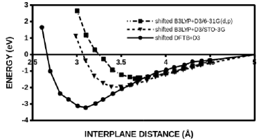
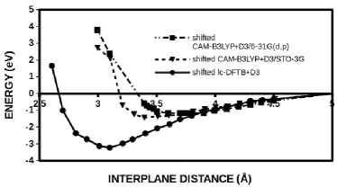
Figure 21: Pentacene tetramer potential energy surfaces with dispersion correction: (a) B3LYP+D3 and DFTB+D3; (b) CAM-B3LYP+D3, lc-DFTB+D3.

Figure 21 shows the improved curves obtained using Grimme’s D3 dispersion correction. The minima are located at at about 3.7 Å for B3LYP+D3, at about 3.72 Å for CAM-B3LYP+D3, and at about 3.1 Å for DFTB+D3.

Table 2: Intermolecular distances obtained for the tetramer of parallel stacked pentacene molecules.

Method	Distance (Å)
LDA/STO-3G	3.7
LDA/6-31G(d,p)	3.6
B3LYP+D3/STO-3G	3.5
B3LYP+D3/6-31G(d,p)	3.68
CAM-B3LYP+D3/STO-3G	3.5
CAM-B3LYP+D3/6-31G(d,p)	3.72
DFTB+D3	3.1
lc-DFTB+D3	3.1

Optimized intermolecular distances are summarized in Table 2.

IV.2.2 Energy versus charge transfer

Now that we have determined an optimal stacking distance (namely 3.71 Å), we can use the analogy to stacked ethylenes developed in the previous section to estimate the relative contributions of CT versus ET in the exciton model. This is possible by concentrating on the central part (carbons 6 and 13 of Fig. 14) of the H($b_{2g}$) and L($b_{3u}$) MOs in Fig. 16. This part of the pentacene H($b_{2g}$) MO resembles the ethylene $\pi^{*}$ MO while the pentacene L($b_{3u}$) MO resembles the ethylene $\pi$ MO (Fig. 2). Figure 19 shows a side view of the pentacene H $\rightarrow$ L transition. Looked at this way, the only important difference between the MOs for stacked pentacenes and the MOs for stacked ethylenes is that one MO diagram is the inverse of the other (i.e., bonding and antibonding orbitals have been interchanged).

Table 3: Relative percentages of CT and ET excitonic transitions to the principle transition for two parallel stacked pentacenes as a function of method. See Eq. (27). DS is the Davydov splitting between the CT and ET excitonic transitions.

Method
State	$f$ (unitless)	$\lambda$ (nm)	$\Delta E$ (eV)	ET	CT
TD-LDA/6-31G(d,p)//LDA/6-31G(d,p)
$1\,^{1}B_{1u}$	0.0002	1033	1.20	0.3%	99.%
$2\,^{1}B_{1u}$	0.0322	733	1.69	99.%	0.3%
			DS2 = 0.49 eV
TD-LDA/STO-3G//LDA/STO-3G
$1\,^{1}B_{1u}$	0.0000	818	1.52	0.005%	99.%
$2\,^{1}B_{1u}$	0.0499	572	2.17	99.%	0.005%
			DS2 = 0.65 eV
TD-B3LYP/6-31G(d,p)//B3LYP+D3/6-31G(d,p)
$1\,^{1}B_{1u}$	0.0005	735	1.69	2.9%	98.%
$2\,^{1}B_{1u}$	0.0576	621	2.00	98.%	2.9%
			DS2 = 0.31 eV
TD-B3LYP/STO-3G//B3LYP+D3/STO-3G
$1\,^{1}B_{1u}$	0.0000	604	2.05	0.02%	100.%
$2\,^{1}B_{1u}$	0.0897	484	2.56	99.%	2.9%
			DS2 = 0.51 eV
TD-DFTB//DFTB+D3
$1\,^{1}B_{1u}$	0.0001	872	1.42	0.05%	100.%
$2\,^{1}B_{1u}$	0.2831	634	1.96	100.%	0.06%
			DS2 = 0.54 eV
TD-CAM-B3LYP/6-31G(d,p)//B3LYP+D3/6-31G(d,p)
$1\,^{1}B_{1u}$	0.1036	523	2.37	97.%	3.%
$2\,^{1}B_{1u}$	0.0033	489	2.54	3.%	97.%
			DS2 = -0.17 eV
TD-CAM-B3LYP/STO-3G//CAM-B3LYP+D3/STO-3G
$1\,^{1}B_{1u}$	0.0004	423	2.93	0.2%	99.%
$2\,^{1}B_{1u}$	0.1628	404	3.07	99.%	0.2%
			DS2 = 0.14 eV
TD-lc-DFTB//lc-DFTB+D3
$1\,^{1}B_{1u}$	0.5782	495	2.50	99.8%	0.24%
$2\,^{1}B_{1u}$	0.0013	451	2.75	0.21%	99.8%
			DS2 = -0.25 eV
TD-HF/6-31G(d,p)//B3LYP+D3/6-31G(d,p)
$1\,^{1}B_{1u}$	0.2087	474	2.62	100.%	0.07%
$2\,^{1}B_{1u}$	0.0002	332	3.73	0.06%	100.%
			DS2 = -1.11 eV
TD-HF/STO-3G//B3LYP+D3/6-31G(d,p)
$1\,^{1}B_{1u}$	0.3557	347	3.58	100.%	0.01%
$2\,^{1}B_{1u}$	0.0001	282	4.40	0.01%	100.%
			DS2 = -0.82 eV

a)
b)

Figure 22: Dimer NTOs and renormalized coefficients: (a) TD-B3LYP/6-31G(d,p)//D3-B3LYP/6-31G(d,p) 621 nm, (b) TD-B3LYP/6-31G(d,p)//D3-B3LYP/6-31G(d,p) 735 nm.

Figure 22 shows the stacked pentacene dimer MOs which may be compared with the stacked ethylene dimer MOs (Fig. 4). It is easy to identify the coefficient $c_{1}$ for the ${}^{1}(H,L+1)$ configuration and the coefficient $c_{2}$ for the ${}^{1}(H-1,L)$ configuration. Table 3 shows how the excitations split into a bright ET exciton and a much darker CT exciton. The energy splitting DS = ET - CT is the Davydov splitting. Our exciton model (Fig. 7)

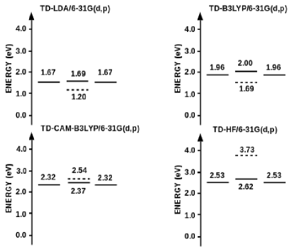
Figure 23: Comparison of exciton diagrams for different functionals using the data from Tables 1 and 3.

predicts a positive DS and this is exactly what is seen in our TD-LDA/6-31G(d,p), TD-LDA/STO-3G, TD-B3LYP/6-31G(d,p), TD-B3LYP/STO-3G, TD-CAM-B3LYP/STO-3G, and TD-DFTB calculations. However, improving the description of charge transfer by adding more HF exchange leads to negative values of DS in the TD-CAM-B3LYP/6-31G(d,p), TD-HF/6-31G(d,p), TD-HF/STO-3G, and TD-lc-DFTB models and a very different picture of exciton coupling (Fig. 23) than that seen in Kasha’s original exciton model. Careful rereading of the classic exciton theory article of Kasha, Rawls, and El-Bayoumi Kasha et al. (1965) reveals that they took into account only dipole-dipole interactions but not charge-transfer effects. As these charge transfer effects are implicit in our calculations, we may explain the observation that Hartree-Fock exchange leads to CT excitonic states of higher energy than ET states by the large amount of energy needed to separate charges. Interestingly the DS obtained from TD-DFTB//DFTB+D3 resembles most closely that obtained with the TD-B3LYP/STO-3G//B3LYP+D3/STO-3G or TD-LDA/STO-3G//LDA+D3/STO-3G, consistent with the idea that the DS is primarily determined by the overlap which is too small when a minimal basis set is used. The situation changes markedly in going to the long-range corrected functionals. Here the TD-lc-DFTB DS is closer to the TD-CAM-DFTB/6-31G(d,p) DS than to the TD-CAM-DFTB/STO-3G DS.

Table 4: Relative percentages of CT and ET excitonic transitions to the principle transition for three parallel stacked pentacenes as a function of method. See Eq. (30). DS is the Davydov splitting between the lowest energy CT and the highest energy ET excitonic transitions.

Method
State	$f$ (unitless)	$\lambda$ (nm)	$\Delta E$ (eV)
TD-LDA/6-31G(d,p)//LDA/6-31G(d,p)
$1\,^{1}B_{1u}$	0.0000	2444	0.51
		Analysis
		100%	1(H,L)
		0%	(ET12+ET23)/$\sqrt{3}$
		0%	($\sqrt{3}/2$)[ET13-(1/3)(ET12+ET23)]
		0%	(CT12+CT23)/$\sqrt{2}$
		0%	CT13
		0%	1(H-2,L+2)
$2\,^{1}B_{1u}$	0.0002	1040	1.20
		Analysis
		0%	1(H,L)
		8.9%	(ET12+ET23)/$\sqrt{3}$
		2.9%	($\sqrt{3}/2$)[ET13-(1/3)(ET12+ET23)]
		81.9%	(CT12+CT23)/$\sqrt{2}$
		6.3%	CT13
		0%	1(H-2,L+2)
$3\,^{1}B_{1u}$	0.0003	950	1.30
		Analysis
		0%	1(H,L)
		1.2%	(ET12+ET23)/$\sqrt{3}$
		34.2%	($\sqrt{3}/2$)[ET13-(1/3)(ET12+ET23)]
		7.6%	(CT12+CT23)/$\sqrt{2}$
		54.6%	CT13
		2.3%	1(H-2,L+2)
$4\,^{1}B_{1u}$	0.0405	730.	1.70
		Analysis
		0%	1(H,L)
		80.6%	(ET12+ET23)/$\sqrt{3}$
		19.1%	($\sqrt{3}/2$)[ET13-(1/3)(ET12+ET23)]
		0.3%	(CT12+CT23)/$\sqrt{2}$
		0.02%	CT13
		0%	1(H-2,L+2)
DS3 = 0.50 eV
TD-LDA/STO-3G//LDA/STO-3G
$1\,^{1}B_{1u}$	0.0000	1024	1.21
		Analysis
		88.4%	1(H,L)
		0.1%	(ET12+ET23)/$\sqrt{3}$
		3.5%	($\sqrt{3}/2$)[ET13-(1/3)(ET12+ET23)]
		2.3%	(CT12+CT23)/$\sqrt{2}$
		5.7%	CT13
		0%	1(H-2,L+2)
$2\,^{1}B_{1u}$	0.0000	816	1.52
		Analysis
		0%	1(H,L)
		0.3%	(ET12+ET23)/$\sqrt{3}$
		7.3%	($\sqrt{3}/2$)[ET13-(1/3)(ET12+ET23)]
		79.7%	(CT12+CT23)/$\sqrt{2}$
		12.7%	CT13
		0%	1(H-2,L+2)
$3\,^{1}B_{1u}$	0.0000	754	1.64
		Analysis
		7.2%	1(H,L)
		0.1%	(ET12+ET23)/$\sqrt{3}$
		39.2%	($\sqrt{3}/2$)[ET13-(1/3)(ET12+ET23)]
		22.8%	(CT12+CT23)/$\sqrt{2}$
		4.1%	CT13
		26.7%	1(H-2,L+2)
$4\,^{1}B_{1u}$	0.0664	571	2.17
		Analysis
		0%	1(H,L)
		78.5%	(ET12+ET23)/$\sqrt{3}$
		21.4%	($\sqrt{3}/2$)[ET13-(1/3)(ET12+ET23)]
		0.05%	(CT12+CT23)/$\sqrt{2}$
		0.05%	CT13
		0%	1(H-2,L+2)
DS3 = 0.65 eV

Table 5: Relative percentages of CT and ET excitonic transitions to the principle transition for three parallel stacked pentacenes as a function of method. See Eq. (30). DS is the Davydov splitting between the lowest energy CT and the highest energy ET excitonic transitions.

Method
State	$f$ (unitless)	$\lambda$ (nm)	$\Delta E$ (eV)
TD-B3LYP/6-31G(d,p)//B3LYP+D3/6-31G(d,p)
$1\,^{1}B_{1u}$	0.0001	1220	1.02
		Analysis
		100.0%	1(H,L)
		0%	(ET12+ET23)/$\sqrt{3}$
		0%	($\sqrt{3}/2$)[ET13-(1/3)(ET12+ET23)]
		0%	(CT12+CT23)/$\sqrt{2}$
		0%	CT13
		0%	1(H-2,L+2)
$2\,^{1}B_{1u}$	0.0006	734	1.69
		Analysis
		0%	1(H,L)
		0.8%	(ET12+ET23)/$\sqrt{3}$
		0%	($\sqrt{3}/2$)[ET13-(1/3)(ET12+ET23)]
		98.8%	(CT12+CT23)/$\sqrt{2}$
		0.3%	CT13
		0%	1(H-2,L+2)
$3\,^{1}B_{1u}$	0.0012	657	1.89
		Analysis
		0%	1(H,L)
		0.6%	(ET12+ET23)/$\sqrt{3}$
		39.7%	($\sqrt{3}/2$)[ET13-(1/3)(ET12+ET23)]
		0.2%	(CT12+CT23)/$\sqrt{2}$
		59.5%	CT13
		0%	1(H-2,L+2)
$4\,^{1}B_{1u}$	0.0723	618	2.01
		Analysis
		0%	1(H,L)
		82.9%	(ET12+ET23)/$\sqrt{3}$
		15.8%	($\sqrt{3}/2$)[ET13-(1/3)(ET12+ET23)]
		0.9%	(CT12+CT23)/$\sqrt{2}$
		0.4%	CT13
		0%	1(H-2,L+2)
DS3 = 0.32 eV
TD-B3LYP/STO-3G//B3LYP+D3/STO-3G
$1\,^{1}B_{1u}$	0.0001	801	1.55
		Analysis
		100%	1(H,L)
		0%	(ET12+ET23)/$\sqrt{3}$
		0%	($\sqrt{3}/2$)[ET13-(1/3)(ET12+ET23)]
		0%	(CT12+CT23)/$\sqrt{2}$
		0%	CT13
		0%	1(H-2,L+2)
$2\,^{1}B_{1u}$	0.0000	602	2.06
		Analysis
		0%	1(H,L)
		0.0%	(ET12+ET23)/$\sqrt{3}$
		0%	($\sqrt{3}/2$)[ET13-(1/3)(ET12+ET23)]
		100.0%	(CT12+CT23)/$\sqrt{2}$
		0.0%	CT13
		0%	1(H-2,L+2)
$3\,^{1}B_{1u}$	0.0003	539	2.30
		Analysis
		0%	1(H,L)
		7.0%	(ET12+ET23)/$\sqrt{3}$
		79.6%	($\sqrt{3}/2$)[ET13-(1/3)(ET12+ET23)]
		0.0%	(CT12+CT23)/$\sqrt{2}$
		13.4%	CT13
		0%	1(H-2,L+2)
$4\,^{1}B_{1u}$	0.1180	482	2.57
		Analysis
		0%	1(H,L)
		82.9%	(ET12+ET23)/$\sqrt{3}$
		17.1%	($\sqrt{3}/2$)[ET13-(1/3)(ET12+ET23)]
		0.0%	(CT12+CT23)/$\sqrt{2}$
		0.0%	CT13
		0%	1(H-2,L+2)
DS3 = 0.51 eV

Table 6: Relative percentages of CT and ET excitonic transitions to the principle transition for three parallel stacked pentacenes as a function of method. See Eq. (30). DS is the Davydov splitting between the lowest energy CT and the highest energy ET excitonic transitions.

Method
State	$f$ (unitless)	$\lambda$ (nm)	$\Delta E$ (eV)
TD-DFTB//DFTB+D3
$1\,^{1}B_{1u}$	0.0000	1606	0.772
		Analysis
		86.9%	1(H,L)
		1.6%	(ET12+ET23)/$\sqrt{3}$
		6.6%	($\sqrt{3}/2$)[ET13-(1/3)(ET12+ET23)]
		0%	(CT12+CT23)/$\sqrt{2}$
		4.9%	CT13
		0%	1(H-2,L+2)
$2\,^{1}B_{1u}$	0.0002	872	1.42
		Analysis
		0%	1(H,L)
		0.01%	(ET12+ET23)/$\sqrt{3}$
		0%	($\sqrt{3}/2$)[ET13-(1/3)(ET12+ET23)]
		99.9%	(CT12+CT23)/$\sqrt{2}$
		0.03%	CT13
		0%	1(H-2,L+2)
$3\,^{1}B_{1u}$	0.0004	819	1.51
		Analysis
		0%	1(H,L)
		6.0%	(ET12+ET23)/$\sqrt{3}$
		39.8%	($\sqrt{3}/2$)[ET13-(1/3)(ET12+ET23)]
		7.5%	(CT12+CT23)/$\sqrt{2}$
		46.7%	CT13
		0%	1(H-2,L+2)
$4\,^{1}B_{1u}$	0.4122	624	1.99
		Analysis
		0%	1(H,L)
		4.2%	(ET12+ET23)/$\sqrt{3}$
		47.6%	($\sqrt{3}/2$)[ET13-(1/3)(ET12+ET23)]
		40.3%	(CT12+CT23)/$\sqrt{2}$
		7.9%	CT13
		0%	1(H-2,L+2)
DS3 = 0.57 eV
TD-CAM-B3LYP/6-31G(d,p)//B3LYP+D3/6-31G(d,p)
$1\,^{1}B_{1u}$	0.0005	764	1.62
		Analysis
		94.5%	1(H,L)
		0.7%	(ET12+ET23)/$\sqrt{3}$
		2.7%	($\sqrt{3}/2$)[ET13-(1/3)(ET12+ET23)]
		0%	(CT12+CT23)/$\sqrt{2}$
		2.0%	CT13
		0%	1(H-2,L+2)
$2\,^{1}B_{1u}$	0.1301	520	2.38
		Analysis
		0%	1(H,L)
		74.4%	(ET12+ET23)/$\sqrt{3}$
		20.6%	($\sqrt{3}/2$)[ET13-(1/3)(ET12+ET23)]
		4.9%	(CT12+CT23)/$\sqrt{2}$
		0.06%	CT13
		0%	1(H-2,L+2)
$3\,^{1}B_{1u}$	0.0074	489	2.53
		Analysis
		0%	1(H,L)
		4.5%	(ET12+ET23)/$\sqrt{3}$
		0%	($\sqrt{3}/2$)[ET13-(1/3)(ET12+ET23)]
		94.0%	(CT12+CT23)/$\sqrt{2}$
		1.5%	CT13
		0%	1(H-2,L+2)
$4\,^{1}B_{1u}$	0.0001	435	2.85
		Analysis
		4.2%	1(H,L)
		2.0%	(ET12+ET23)/$\sqrt{3}$
		22.9%	($\sqrt{3}/2$)[ET13-(1/3)(ET12+ET23)]
		7.9%	(CT12+CT23)/$\sqrt{2}$
		40.3%	CT13
		22.7%	1(H-2,L+2)
DS3 = -0.15 eV

Table 7: Relative percentages of CT and ET excitonic transitions to the principle transition for three parallel stacked pentacenes as a function of method. See Eq. (30). DS is the Davydov splitting between the lowest energy CT and the highest energy ET excitonic transitions.

Method
State	$f$ (unitless)	$\lambda$ (nm)	$\Delta E$ (eV)
TD-CAM-B3LYP/STO-3G//CAM-B3LYP+D3/STO-3G
$1\,^{1}B_{1u}$	0.0006	544	2.28
		Analysis
		93.0%	1(H,L)
		4.1%	(ET12+ET23)/$\sqrt{3}$
		1.7%	($\sqrt{3}/2$)[ET13-(1/3)(ET12+ET23)]
		0%	(CT12+CT23)/$\sqrt{2}$
		1.2%	CT13
		0%	1(H-2,L+2)
$2\,^{1}B_{1u}$	0.0000	423	2.93
		Analysis
		0%	1(H,L)
		4.4%	(ET12+ET23)/$\sqrt{3}$
		0%	($\sqrt{3}/2$)[ET13-(1/3)(ET12+ET23)]
		89.7%	(CT12+CT23)/$\sqrt{2}$
		5.9%	CT13
		0%	1(H-2,L+2)
$3\,^{1}B_{1u}$	0.2165	402	3.08
		Analysis
		0%	1(H,L)
		79.6%	(ET12+ET23)/$\sqrt{3}$
		20.3%	($\sqrt{3}/2$)[ET13-(1/3)(ET12+ET23)]
		0.03%	(CT12+CT23)/$\sqrt{2}$
		0.1%	CT13
		0%	1(H-2,L+2)
$4\,^{1}B_{1u}$	0.0001	371	3.34
		Analysis
		0%	1(H,L)
		3.4%	(ET12+ET23)/$\sqrt{3}$
		23.9%	($\sqrt{3}/2$)[ET13-(1/3)(ET12+ET23)]
		0.7%	(CT12+CT23)/$\sqrt{2}$
		45.1%	CT13
		26.8%	1(H-2,L+2)
DS3 = 0.15 eV
TD-lc-DFTB//lc-DFTB+D3
$1\,^{1}B_{1u}$	0.0028	705	1.76
		Analysis
		88.4%	1(H,L)
		1.5%	(ET12+ET23)/$\sqrt{3}$
		5.8%	($\sqrt{3}/2$)[ET13-(1/3)(ET12+ET23)]
		0%	(CT12+CT23)/$\sqrt{2}$
		4.4%	CT13
		0%	1(H-2,L+2)
$2\,^{1}B_{1u}$	0.8238	487	2.54
		Analysis
		0%	1(H,L)
		29.6%	(ET12+ET23)/$\sqrt{3}$
		26.0%	($\sqrt{3}/2$)[ET13-(1/3)(ET12+ET23)]
		14.2%	(CT12+CT23)/$\sqrt{2}$
		30.2%	CT13
		0%	1(H-2,L+2)
$3\,^{1}B_{1u}$	0.0018	452	2.74
		Analysis
		0%	1(H,L)
		0.01%	(ET12+ET23)/$\sqrt{3}$
		0%	($\sqrt{3}/2$)[ET13-(1/3)(ET12+ET23)]
		100.0%	(CT12+CT23)/$\sqrt{2}$
		0.003%	CT13
		0%	1(H-2,L+2)
$4\,^{1}B_{1u}$	0.0007	409	3.03
		Analysis
		0%	1(H,L)
		3.8%	(ET12+ET23)/$\sqrt{3}$
		15.2%	($\sqrt{3}/2$)[ET13-(1/3)(ET12+ET23)]
		0%	(CT12+CT23)/$\sqrt{2}$
		11.4%	CT13
		69.5%	1(H-2,L+2)
DS3 = -0.20 eV

Table 8: Relative percentages of CT and ET excitonic transitions to the principle transition for three parallel stacked pentacenes as a function of method. See Eq. (30). DS is the Davydov splitting between the lowest energy CT and the highest energy ET excitonic transitions.

Method
State	$f$ (unitless)	$\lambda$ (nm)	$\Delta E$ (eV)
TD-HF/STO-3G//B3LYP+D3/6-31G(d,p)
$1\,^{1}B_{1u}$	0.0051	417	2.97
		Analysis
		77.8%	1(H,L)
		0.2%	(ET12+ET23)/$\sqrt{3}$
		8.4%	($\sqrt{3}/2$)[ET13-(1/3)(ET12+ET23)]
		1.4%	(CT12+CT23)/$\sqrt{2}$
		9.6%	CT13
		6.9%	1(H-2,L+2)
$2\,^{1}B_{1u}$	0.4703	343	3.62
		Analysis
		0%	1(H,L)
		89.4%	(ET12+ET23)/$\sqrt{3}$
		21.2%	($\sqrt{3}/2$)[ET13-(1/3)(ET12+ET23)]
		0.02%	(CT12+CT23)/$\sqrt{2}$
		0.02%	CT13
		0%	1(H-2,L+2)
$3\,^{1}B_{1u}$	0.0001	283	4.38
		Analysis
		4.3%	1(H,L)
		0.65%	(ET12+ET23)/$\sqrt{3}$
		0%	($\sqrt{3}/2$)[ET13-(1/3)(ET12+ET23)]
		91.1%	(CT12+CT23)/$\sqrt{2}$
		0.22%	CT13
		3.7%	1(H-2,L+2)
$4\,^{1}B_{1u}$	0.0000	270	4.59
		Analysis
		18.3%	1(H,L)
		1.3%	(ET12+ET23)/$\sqrt{3}$
		9.5%	($\sqrt{3}/2$)[ET13-(1/3)(ET12+ET23)]
		9.5%	(CT12+CT23)/$\sqrt{2}$
		17.8%	CT13
		48.4%	1(H-2,L+2)
DS3 = -1.06 eV
TD-HF/6-31G(d,p)//B3LYP+D3/6-31G(d,p)
$1\,^{1}B_{1u}$	0.0025	662	1.87
		Analysis
		81.0%	1(H,L)
		0.2%	(ET12+ET23)/$\sqrt{3}$
		7.1%	($\sqrt{3}/2$)[ET13-(1/3)(ET12+ET23)]
		3.1%	(CT12+CT23)/$\sqrt{2}$
		13.9%	CT13
		0%	1(H-2,L+2)
$2\,^{1}B_{1u}$	0.2682	468	2.65
		Analysis
		0%	1(H,L)
		89.0%	(ET12+ET23)/$\sqrt{3}$
		21.8%	($\sqrt{3}/2$)[ET13-(1/3)(ET12+ET23)]
		0.11%	(CT12+CT23)/$\sqrt{2}$
		0.003%	CT13
		0%	1(H-2,L+2)
$3\,^{1}B_{1u}$	0.0002	334	3.71
		Analysis
		4.0%	1(H,L)
		1.5%	(ET12+ET23)/$\sqrt{3}$
		0.%	($\sqrt{3}/2$)[ET13-(1/3)(ET12+ET23)]
		90.6%	(CT12+CT23)/$\sqrt{2}$
		5.1%	CT13
		3.4%	1(H-2,L+2)
$4\,^{1}B_{1u}$	0.0004	315	3.94
		Analysis
		18.1%	1(H,L)
		1.1%	(ET12+ET23)/$\sqrt{3}$
		14.7%	($\sqrt{3}/2$)[ET13-(1/3)(ET12+ET23)]
		11.5%	(CT12+CT23)/$\sqrt{2}$
		25.1%	CT13
		36.8%	1(H-2,L+2)
DS3 = -0.76 eV

Tables 4, 5, 6, 7, and 8 apply the analysis of Sec. II to the equally-spaced parallel stacked trimer. As expected, instead of a Davydov pair of ET and CT excitations, we find a Davydov triplet corresponding to the $2\,^{1}B_{1u}$, $3\,^{1}B_{1u}$, and $4\,^{1}B_{1u}$ states. When the Davydov pairs can be identified, we have highlighted their assignment in terms of nearest neighbor interactions in bold face in the tables. Cases where the Davydov pairs are clear are: TD-LDA/6-31G(d,p)//LDA/6-31G(d,p), TD-LDA/STO-3G//LDA/STO-3G, TD-B3LYP/6-31G(d,p)//B3LYP+D3/6-31G(d,p), TD-B3LYP/STO-3G//B3LYP+D3/STO-3G, TD-DFTB//DFTB+D3. In these cases, the (ET₁₂+ET₂₃)-dominated state is the highest energy transition of the Davydov triplet and also has the highest oscillator strength while the (CT₁₂+CT₂₃)-dominated state is the lowest energy transition of the Davydov triplet and has significantly less oscillator strength. A third contribution to the Davydov triplet lies between the two other states and also has only a feeble transition energy. This assignment is a bit less clear in the TD-DFTB//DFTB+D3 case because there is significant mixing between ET₁₂+ET₂₃ and ET₁₃ in the brightest configuration. Henceforth we shall simply assume that the peak with the highest oscillator strength is an (ET₁₂+ET₂₃)-dominated state.

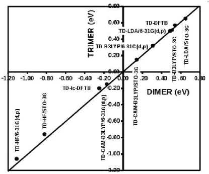
Figure 24: Graph comparing the Davydov splittings, $E$(ET)-$E$(CT), of the trimer and dimer. The 45^∘ line indicates perfect agreement between dimer and trimer Davydov splittings.

Figure 24 shows that calculations with these methods give essentially the same Davydov splitting for the dimer and for the trimer, and that the dimer (DS₂) and trimer (DS₃) splittings are very similar for TD-DFTB and for TD-B3LYP/6-31G(d,p), as well as being very similar for TD-lc-DFT and for TD-CAM-B3LYP/6-31G(d,p).

IV.2.3 Spectra

a)
b)
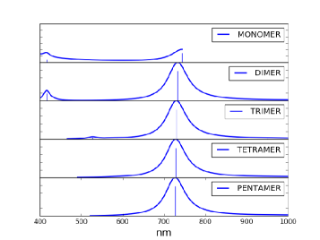
c)
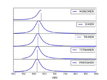
d)

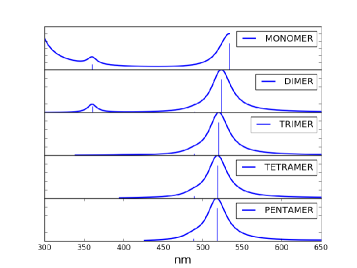
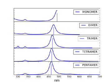
Figure 25: Convergence of spectra as a function of number of pentacene molecules in the stack: (a) TD-LDA/6-31G(d,p), (b) TD-B3LYP/6-31G(d,p), (c) TD-CAM-B3LYP/6-31G(d,p), and (d) TD-HF/6-31G(d,p).

Calculations beyond the trimer become increasingly complicated to analyze but we may compare calculated spectra for increasingly large numbers of parallel stacked pentacene molecules. The tight-binding calculation in Sec. II is based upon the hope that nearest neighbor interactions dominate excitonic effects in spectra. The comparison of dimer and trimer DSs seem to at least partially confirm this. We may make a further check by seeing how the spectra change as more and more pentacene molecules are stacked. These spectra are shown in Fig. 25. All of the spectra show a main peak (i.e., the ET peak) which blue shifts as the pentacene stack grows. More specifically, the graphs show a main peak which undergoes the largest shift in going from the monomer to the dimer, a smaller shift in going from the dimer to the trimer and then shifts very little in going to higher oligomers, consistent with the suppositions behind the tight-binding model.

a)
b)

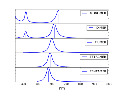
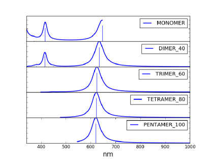
Figure 26: TD-DFTB spectra of stacked pentacene: (a) with a fixed active space, (b) with a size-extensive active space.

a)
b)

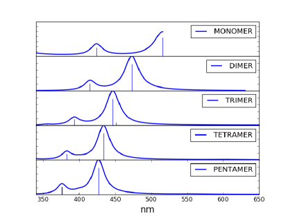
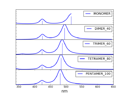
Figure 27: TD-lc-DFTB spectra of stacked pentacene: (a) with a fixed active space, (b) with a size-consistent active space.

Our TD-DFT and TD-lc-DFTB calculations led us to become aware of a problem already reported in Ref. Humeniuk and Mitrič, 2017. It is in the spirit of semi-empirical approaches to make simplifying approximations which allow the treatment of larger molecules than would otherwise be possible. This is why DFTBaby restricts the space of active orbitals, but it is still up to the user to decide how to use this option. One way would be to increase the size of the active space until converged spectra are achieved. But this ideal approach is not really practical when going to larger and larger aggregates of molecules. Instead, the first idea that comes to mind is to use the largest active space for which calculations are possible. In practice, this means using the same number of occupied and unoccupied orbitals in the active space, independent of the number of molecules. We call doing this a calculation with a fixed active space. However it has the important drawback when describing size-dependent trends that fixed active space calculations have more basis functions per molecule for smaller aggregates than for larger aggregates and so invariably describe smaller aggregates better than larger aggregates with the introduction of corresponding systematic errors in the resultant size-dependent properties. The other approach is to keep the number of occupied and unoccupied orbitals in the active space proportional to the number of molecules. In this way, we hope to obtain a better description of size-dependent trends, albeit at some cost of accuracy for smaller aggregats. We call this doing a calculation with a size-consistent active space. (There is some confusion in the literature between the terms “size-consistent” and “size-extensive.” Both terms are arguably correct here, but we shall stick to “size-consistent.”)

(Our size-consistent active-space approach resembles other approaches based upon energy and/or oscillator strength cut-offs Domínguez García (2014); Rüger et al. (2015). Note however that there is an important difference in philosophy as the latter aim for accurage spectra with large basis sets while our approach aims at constant accuracy for varying sizes of aggregates.)

Figures 26 and 27 compare fixed and size-consistent active space calculations. The fixed active space calculations use 20 occupied orbitals and 20 unoccupied orbitals per aggregate. The size-consistent active space calculations use 20 occupied and 20 unoccupied orbitals per pentacene molecule. As the figure shows, the calculations with fixed active space blue shifts much more than do the calculations with self-consistent active space as the number of pentacene molecules increases. TD-DFT calculations of excitation energies are variational in the Tamm-Dancoff approximation and pseudo-variational in the sense that full linear response calculations often give similar results to using the Tamm-Dancoff approximation. For the monomer the fixed active space and size-consistent active space calculations are identical; however for the aggregates, the size-consistent active space is larger than the fixed active space calculations, leading to lower excitation energies in the size-consistent active space calculations. One would hope that the larger basis set would give better and answers and that this is the case is shown in Fig. 28 where it is seen that TD-DFTB and TD-B3LYP/6-31G(d,p) spectral peak locations differ by only about 10 nm. Figure 26 shows that the difference between the TD-DFTB and TD-B3LYP/6-31G(d,p) calculations would have been more like 50 nm had the fixed active space been used. Figure 28 also shows that the differences between TD-lc-DFTB and TD-CAM-B3LYP/6-31G(d,p) spectra are larger than for the TD-DFTB and TD-B3LYP/6-31G(d,p) case when the size-extensive active space is used, with the main peak in this part of the spectrum having an energy difference of around 30 nm between the two calculations. Interestingly both show qualitatively similar Davydov multiplets. Figure 27 shows that the difference between the TD-lc-DFTB and TD-CAM-B3LYP(d,p) calculations would have been more like 80 nm had the fixed active space been used. This is why, except for Figs. 26 and 27, we have been careful to use a size-consistent active space consisting of 20 occupied and 20 unoccupied orbitals per molecule in all the TD-DFTB and TD-lc-DFTB reported in this paper.

a)
b)

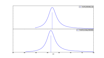
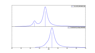
Figure 28: Comparison of pentacene spectra: (a) TD-DFTB and TD-B3LYP/6-31G(d,p) and (b) TD-lc-DFTB and TD-CAM-B3LYP/6-31G(d,p).

IV.3 Herringbone

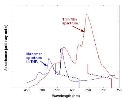
Figure 29: Excitonic effects on the absorption spectrum of pentacene: curves, pentacene in tetrahydrofuran (THF) and as a thin film (from Ref. Maliakal et al., 2004); stick spectra, lower are the position of unshifted monomer and crystal peaks calculated using the Bethe-Salpeter equation (BSE) while the upper stick spectra have been shifted to match the experiment (from Ref. Cudazzo et al., 2015.) See also Ref. Tiago et al., 2003.

The main objective of the present work has been to evaluate the ability of TD-DFTB and TD-lc-DFTB to simulate, respectively, the results of TD-B3LYP/6-31G(d,p) and TD-CAM-B3LYP/6-31G(d,p) calculations. While this has been largely satisfied by our study of parallel stacked pentacene molecules, the case of parallel stacked molecules is too artificial to allow comparison against experiment (except for the monomer.) In order to have a reality check, we have also carried out calculations for cluster models of pentacene crystals. The experimental spectrum of the molecule and of the crystal are available both from experiment Sebastian et al. (1981); Maliakal et al. (2004); Hestand et al. (2015) and from state-of-the-art theoretical calculations Tiago et al. (2003); Ambrosch-Draxl et al. (2009); Cudazzo et al. (2013); Sharifzadeh et al. (2013); Cudazzo et al. (2015). These are shown in Fig. 29. This time excitonic shifts lead to a red shift, rather than a blue shift. The structure of the spectrum suggests that both CT and ET transitions contribute to the spectrum. As we shall see, charge transfer is more important for describing excitonic effects in the absorption spectrum than is the case for parallel stacked pentamers.

a)
b)
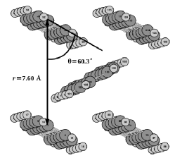
c)

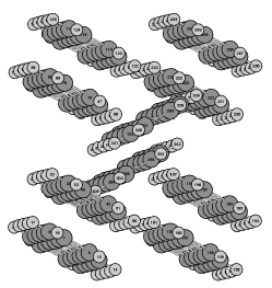
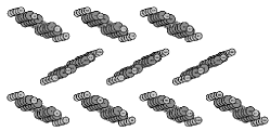
Figure 30: Herringbone cluster models used in this work. All are portions of the x-ray crystal structure: (a) pentamer, (b) “vertical” decamer, and (c) “horizontal” decamer.

We carried out calculations for the cluster models shown in Fig. 30 obtained by cutting out different portions of the x-ray crystal structure Dorset and McCourt (1994); Schiefer et al. (2007) without any subsequent relaxation. Unless otherwise indicated all of the results reported below are for the “horizontal” decamer model. The picture of the horizontal model makes it clear that the crystal is made up of layers of tilted stacks of pentamers whose tilt angles alternate from layer to layer to provide a herringbone structure.

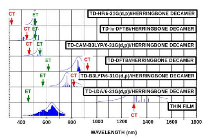
Figure 31: Comparisons of calculations using various methods with the thin film absorption spectrum from Ref. Maliakal et al., 2004. The CT and ET excitation energies were calculated from Kasha’s exciton model using Eq. (116).

Figure 31 shows the herringbone spectra calculated at various levels and compared with the thin film spectrum. Both the TD-LDA/6-31G(d,p) and the TD-B3LYP/6-31G(d,p) calculations are red shifted compared to the thin film experiment with the TD-LDA/6-31G(d,p) red shift being quite dramatic. This is consistent with the idea that the TD-LDA/6-31G(d,p) exciton is delocalized over too many molecules while the inclusion of some HF exchange in the TD-B3LYP/6-31G(d,p) helps to increase the excitation energy by localizing the exciton over fewer molecules. The TD-DFTB calculation is in semi-quantitative agreement with the TD-B3LYP/6-31G(d,p) but are slightly red-shifted. In contrast, the TD-CAM-B3LYP/6-31G(d,p) and TD-HF/6-31G(d,p) calculations are blue shifted compared to the thin film experiment. The TD-lc-DFTB calculation is in semi-quantitative agreement with the TD-CAM-B3LYP/6-31G(d,p) calculation but is slightly blue shifted. It is difficult to say from this figure which of the two calculations — TD-B3LYP/6-31G(d,p) or TD-CAM-B3LYP/6-31G(d,p) — is a better description of the experiment.

a)
b)
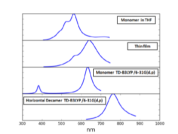
c)
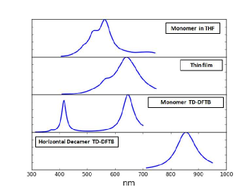
d)

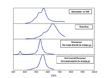
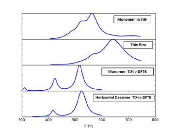
Figure 32: Comparison of theoretical and experimental exciton shifts: (a) TD-B3LYP/6-31G(d,p), (b) TD-DFTB, (c) TD-CAM-B3LYP/6-31G(d,p), and (d) TD-lc-DFTB.

The level of agreement with experiment is best judged by Fig. 32. Here we see that the TD-B3LYP/6-31G(d,p) and TD-DFTB results are in resonable qualitative agreement with experiment. However the TD-CAM-B3LYP/6-31G(d,p) and TD-lc-DFTB results, while in good agreement with each other, do not at all provide a good description of exciton effects. We assume that this is because of the importance of CT which may be over corrected at the TD-CAM-B3LYP/6-31G(d,p) and TD-lc-DFTB levels compared with the TD-B3LYP/6-31G(d,p) and TD-DFTB levels.

IV.4 Re-examination of Kasha’s Model

There is some hope in the literature that you only need to apply Kasha’s original model to a single crystal plane to calculate the Davydov splitting of the crystal Philpott (1973); Yamagata et al. (2011); Meyenburg et al. (2016). In their recent work Meyenburg et al. (2016), Meyenburg et al. give the formula [their Eq. (5) rewritten in atomic units],

$$\Delta E=\frac{2|{\vec{\mu}}^{I0}|^{2}}{\epsilon r^{3}}\left[\cos(\phi)-3\cos(\alpha_{1})\cos(\alpha_{2})\right]\,,$$ (115)

where the angles are defined in Fig. 3 of their paper. [Equation (115) is a generalization of a formula given in the paper of Kasha, Rawls, and El-Bayoumi Kasha et al. (1965) (resulting in Fig. 4 of their article).] We translate this the following relationship between the DS of the herringbone model DS${}_{\text{HB}}$ and of the parallel stack model DS${}_{\text{PS}}$:

DS$${}_{\text{HB}} = \mbox{DS${}_{\text{PS}}$}\left(\frac{\epsilon_{\text{PS}}}{\epsilon_{\text{HB}}}\right)\left(\frac{r_{\text{PS}}}{r_{\text{HB}}}\right)^{3}$$ (116)

$$\times \left[\cos(\phi)-3\cos(\alpha_{1})\cos(\alpha_{2})\right]\,.$$

The values $\alpha_{1}=98.19^{\circ}$, $\alpha_{2}=22.98^{\circ}$, $\phi=58.83^{\circ}$, and $r=4.835$ Å were taken from the experimental crystal structure. The ratio $\epsilon_{\text{PS}}/\epsilon_{\text{HB}}$ is not something that we can really determine a priori and so we just use it as a fitting factor (equal to 10.64 in our calculations). We can use this, together with DS₂ (from our model) to predict the DS${}_{\text{HB}}$ that we would expect from various models. These results are shown by arrows in Fig. 31. Something very remarkable has happened: The locations of the TD-lc-DFTB, TD-HF, and TD-CAM-B3LYP main peaks are well produced, as expected, by the ET peak. In contrast, the location of the TD-DFTB, TD-B3LYP, and TD-LDA main peaks has been generated unexpectedly, from the CT peak, which was expected to be relatively dark compared to the ET peak. This illustrates how easy it is to get the “right answer for the wrong reason.” In particular, applying Kasha’s original exciton model to results from our exciton model gives results which seem reasonable (albeit only with a physically-unreasonable value of the dielectric constant).

a)
b)
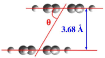
c)

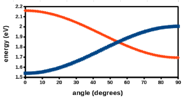
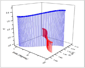
Figure 33: Ideal Kasha figures for co-planar inclined transition dipole moments: (a) laterally shifted parallel stacked pentacene dimer, (b) Kasha plot of excitation energies as a function of the angle $\theta$, (c) 3D plot of Kasha’s model for oscillator strengths and excitation energies.

This leads us to take a closer look at how Kasha’s exciton model compares to our (TD-)DFT and (TD-)DFTB calculations. We have done this by looking at two parallel-stacked pentacenes. This corresponds to a simplification of Eq. (116), namely

$$\Delta E=\frac{2|{\vec{\mu}^{I0}}|^{2}}{r^{3}}\left(1-3\cos^{2}\theta\right)\,,$$ (117)

with $\epsilon=1$. Figure 33 summarizes what we expect to see on the basis of the original exciton model for excitation energies and oscillator strengths. This is a simple theory which gives simple curves. Above $\theta=55^{\circ}$, the main oscillator strength is in the higher energy (lower wavelength) ET state; below $\theta=55^{\circ}$, the main oscillator strength is in the lower energy (higher wavelength) ET state which has crossed the CT state. However the original theory did not anticipate avoided crossings. For the herringbone structure, $\theta\approx 60^{\circ}$ and the prediction is that the brighter state should be the higher wavelength state. This is indeed what is seen in all the calculations in Fig. 31, but the assignment of the longer wavelength peak depends upon the method.

a)
b)
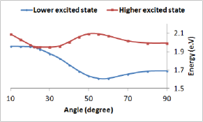
c)

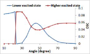
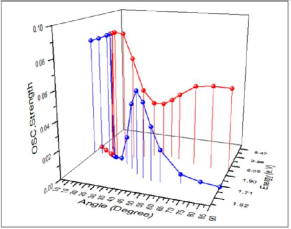
Figure 34: TD-B3LYP/6-31G(d,p)//B3LYP+D3/6-31G(d,p) Kasha figures for co-planar inclined transition dipole moments: (a) excitation energies as a function of the angle $\theta$, (b) 2D plot of oscillator strengths, (c) 3D plot of oscillator strengths and excitation energies,

Let us turn now to Fig. 34 which shows results from our TD-B3LYP/6-31G(d,p)//B3LYP+D3/6-31G(d,p) calculations. This more realistic calculation gives more complicated results. Rather than seeing a simple crossing of energy levels at about $\theta=55^{\circ}$ as in Fig. 33(b), we see evidence of configuration mixing as the oscillator strength is transfered from one state to antother with maximum transfer near $\theta=55^{\circ}$ (i.e., at $\theta=45^{\circ}$) as the two energy levels mix and move apart at $\theta=55^{\circ}$. This seems even more clear in the 3D plot [part (c) of Fig. 34] where the two curves behave in a way very consistent with an avoided crossing of two diabatic states (one with high and one with low oscillator strength) around $50^{\circ}$. Later, at a much lower value of $\theta=20^{\circ}$, there appears to be a real crossing, but this is of little importance for understanding the herringbone results. Comparing with the TD-DFTB, TD-B3LYP, and TD-LDA herringbone spectra in Fig. 31, we realize that the assignment of the longer wavelength peak as CT is misleading as most likely there is a great deal of mixing between the ET and CT states.

a)
b)
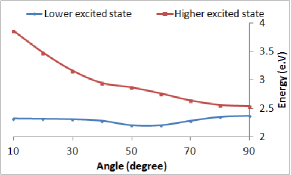
c)

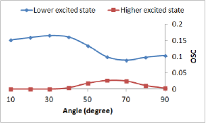
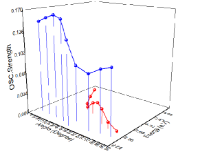
Figure 35: TD-CAM-B3LYP/6-31G(d,p)//CAM-B3LYP+D3/6-31G(d,p) Kasha figures for co-planar inclined transition dipole moments: (a) excitation energies as a function of the angle $\theta$, (b) 2D plot of oscillator strengths, (c) 3D plot of oscillator strengths and excitation energies,

Figure 35 shows what happens for a RSH. In particular, TD-CAM-B3LYP/6-31G(d,p)//CAM-B3LYP+D3/6-31G(d,p) results are shown. There is also some evidence of an avoided crossing here, but the lower energy (longer wavelength) state keeps most of the oscillator strength. At $\theta=90^{\circ}$, it is of ET type, but shows some mixing between CT and ET type at around $\theta=65^{\circ}$. Comparing with the TD-lc-DFTB, TD-HF, and TD-CAM-B3LYP herringbone spectra in Fig. 31, we realize that the assignment of the longer wavelength peak as ET is reasonable in this case.

Despite these criticisms that Kasha’s original exciton model is missing many of the subtleties of our more elaborate calculations, we must conclude that the exciton model allows us to extrapolate remarkably well from intramolecular interactions between pairs of molecules to larger aggregates, but only when a RSH is used.

V Conclusion

The aggregation of dye molecules leads to additional spectral features which have long been explained by Kasha’s exciton model Kasha et al. (1965). This model provides a simple explanation of H-bands such as those found in our calculations of parallel stacked pentacene molecules and of J-bands such as those associated with the experimentally-known herringbone structure of crystalline pentacene. We have re-examined exciton effects on spectra in terms of state-of-the-art TD-DFT and TD-DFTB calculations. Our calculations include Grimme’s D3 dispersion correction which we confirm is absolutely necessary in order to have van der Waals binding beyond the LDA level (which, however, “accidently” binds when an extensive-enough basis set is used). We have also included some HF exchange either in the form of the global B3LYP hybrid functional or in the form of the range-separated CAM-B3LYP hybrid functional. Corresponding TD-DFTB calculations have also been performed with DFTbaby which we find does very well at mimicking the two functionals (depending upon whether or not the long-range correction is used).

Perhaps not surprisingly we find that the hybrid functionals give better spectra than the TD-LDA. We also find that, while the TD-DFTB spectra have the structural simplicity of STO-3G minimum basis set TD-DFT spectra, the TD-DFTB spectral peak energies are placed more like the TD-DFT calculations with larger basis used in the semi-empirical parameterization. This is reassuring. However care must be taken when doing TD-DFTB calculations on aggregates to do them size consistently or results can be misleading — that is, the size of the active space must increase in proportion to the number of molecules in the aggregate.

On the other hand, Fig. 32 is definitely telling us that the Davydov splitting for the herringbone model is reasonable and close to the experimental value at the TD-B3LYP and TD-DFTB levels, even if the spectral peaks are shifted, but that the Davydov splitting is practically nonexistant and therefore wrong at the CAM-TD-B3LYP and TD-lc-DFTB levels. For this reason, we cannot recommend using either of these latter two approaches for calculating excitonic effects on the spectra of polyoligocenes and recommend instead the use of TD-B3LYP or TD-DFTB carefully carried out on aggregates.

Also, in light of arguments regarding the extent and nature of exciton delocalization (e.g., Refs. Zimmerman et al., 2009; Mewes et al., 2017), it is interesting that our analysis shows that a more sophisticated version of Kasha’s exciton model, based only on nearest neighbor interactions but including both ET and CT as well as avoided crossings, works very well. In contrast, Kasha’s original model without further modification fails because of its absence of CT excitations.

It is perhaps not misplaced to say a brief word about some of the many challenges of describing ET and CT excitons that are important for organic electronics but which have not been addressed in this paper. One is the need to take into account the more extended environment. This was only included approximately here in our “Kasha model calculation” by invoking an environmental dielectric constant. It really should be done more correctly and in such a way as to recognize that the effect will be different depending upon the ET and CT nature of the exciton. Furthermore, as we have seen with the RSH functionals, excitons may be of a strongly mixed ET/CT nature whose precise mixture may depend upon environmental effects. Finally, in many organic electronic problems there is an interface with local states which must couple with bulk states. Finding the correct coupling between these two types of states is nontrivial, especially if the goal is to describe both states at the same level of theory. Nevertheless, with all of these caveats, we believe that the present article represents a helpful step towards the practical investigation of realistic models for organic electronics.

Appendix A DFT

Hohenberg-Kohn-Sham DFT Hohenberg and Kohn (1964); Kohn and Sham (1965) is now so well-known that little needs to be said about the basics. For those seeking a deeper understanding of the foundations of DFT, we can recommend Refs. Parr and Yang, 1989; Dreizler and Gross, 1990; Koch and Holthausen, 2000. Our intent here is two fold. Partly we wish to go beyond what is found in those references and partly we wish to review that part of the basics which is needed to understand DFTB.

The fundamental idea of DFT is to replace the real system of $N$ interacting electrons in an external potential $v_{\text{ext}}$ with a fictitious system of $N$ noninteracting electrons in an effective potential $v_{s}$ ($s$ for single electron). We will designate the orbitals of the noninteracting system as $\psi_{i}$ and their associated occupation numbers as $n_{i}$. These orbitals are orthonormal, $\langle\psi_{i}|\psi_{j}\rangle=\delta_{i,j}$. Normally $n_{i}$ is zero or one but fractional occupation is also allowed. The density matrix for the noninteracting system is then, $\gamma(1,2)=\sum_{i}\psi_{i}(1)n_{i}\psi_{i}^{*}(2)$, where the numeral $i=1,2,\cdots$ stands for the space and spin coordinates of the $i$th electron. The density, $\rho(1)=\gamma(1,1)$, is the diagonal element of the density matrix. The electronic energy $E$ is the same for the real and for the interacting systems. It may be written as the sum of three terms,

$$E=E_{c}+E_{H}+E_{xc}\,,$$ (118)

where the core energy $E_{c}$ is the expectation value of the core hamiltonian, $\hat{h}_{c}=-\frac{1}{2}\nabla^{2}+v_{\text{ext}}$, the Hartree energy (also called the classical coulomb repulsion energy) $E_{H}$ denotes the classical repulsion between $\rho$ and itself, and the remaining terms needed to make the electronic energy exact are included in the exchange-correlation (xc) energy, $E_{xc}=E-E_{c}-E_{H}$. This term is approximated in practical calculations. We will consider these approximations very soon. For now, let us note that minimizing $E$ subject to the orbital orthonormality condition leads to an orbital equation,

$$\hat{f}\psi_{i}=\epsilon_{i}\psi_{i}\,,$$ (119)

where $\hat{f}=\hat{h}_{c}+v_{H}+v_{xc}$. Here $v_{H}(1)=\int\rho(2)/r_{12}\,d2$ is the Hartree potential and $v_{xc}(1)=\delta E_{xc}/\delta\rho(1)$ is the xc potential. Then it is easy to see that the effective potential of the noninteracting system is, $v_{s}=v_{\text{ext}}+v_{H}+v_{xc}$. The orbital equation (119) must be solved self-consistently because $\hat{f}$ is orbital dependent. Once self-consistency has been reached, then the energy may be calculated either using Eq. (118) or by using the equation

$$E=\sum_{i}n_{i}\epsilon_{i}-\frac{1}{2}E_{H}+E_{xc}-\int v_{xc}(1)\rho(1)\,d1$$ (120)

This latter form is used as the basis of DFTB.

Thus far the equations are exact, but useless unless approximations are made. We give a brief review of the approximate functionals used in this paper beginning from the most well-known and ending with the range-separated hybrids which play a central role in this paper.

The most common approximation is the local (spin) density approximation (LDA) which assumes that the xc energy density in a nonhomogeneous system such as an atom, molecule, or solid, is the same as the xc energy density in the homogeneous electron gas (HEG), $E_{xc}^{\text{LDA}}=\int\epsilon_{xc}^{\text{HEG}}(\rho(1))\rho(1)\,d1$. The exchange part of $\epsilon_{xc}^{\text{HEG}}$ has a simple analytic form Dirac (1930). We will use the Vosko-Wilk-Nusair parameterization of the correlation part of $\epsilon_{xc}^{\text{HEG}}$ Vosko et al. (1980) in the present work. Strictly speaking all of our calculations have an explicit dependence on the spin polarization of the local density. That is, we are using spin DFT rather than the original DFT which depended only on the spinless charge density.

The LDA often gives reasonable molecular geometries but is known to overbind. For this reason, it has been useful to include inhomogeneities in the density via generalized gradient approximations (GGAs) of the form, $E_{xc}^{\text{GGA}}=\int\epsilon_{xc}^{\text{HEG}}(\rho(1))F_{xc}^{\text{GGA}}(\rho(1),x(1))\rho(1)\,d1$, where the enhancement factor $F_{xc}$ depends both on the local density and upon the local reduced gradient, $x=|\vec{\nabla}\rho|/\rho^{4/3}$. Relevant GGAs used in our calculations are Becke’s 1988 (B88) exchange GGA Becke (1988); Fan and Ziegler (1991), Perdew’s 1991 correlation GGA Perdew et al. (1992, 1993, 1996a, 1996b), and the Lee, Yang, and Parr (LYP) correlation GGA Lee et al. (1988).

Up to this point, the discussion has been limited to pure density functionals — that is, those that depend only upon the charge density. In 1993, Becke introduced some “exact exchange” into the xc functional Becke (1993) (exact exchange is HF exchange evaluated with DFT orbitals.) He did this based upon an adiabatic connection formalism and the improvement in computational results was very striking in that time as they suggested that such (global) hybrid functionals could provide thermochemical accuracy. Of course, this also leaves the framework of formal Hohenberg-Kohn-Sham theory Gill (2001) and we must now speak of generalized Kohn-Sham theory. In particular, the xc energy is now a functional of the density matrix $E[\gamma]$ rather than just the density ($E[\rho]$) and the xc potential becomes an xc operator defined by ${\hat{v}}_{xc}\psi(1)=\int(\delta E_{xc}/\delta\gamma(2,1))\gamma(1,2)\psi_{i}(2)\,d2$. Note that the HF exchange-only operator may be regarded as an extreme case of a global hybrid: $\delta E_{x}^{\text{HF}}[\gamma]/\delta\gamma(2,1)=-\frac{\gamma(1,2)}{r_{1,2}}$. Equation (120) still holds but with a nonlocal $\hat{v}_{xc}$. We use the B3LYP functional in the present work B3L . This is the same as the B3P91 functional originally introduced by Becke Becke (1993) but with Perdew’s 1991 correlation GGA replaced by the LYP correlation GGA. Specifically, $E_{xc}=E_{x}^{\text{LDA}}+a_{0}\left(E_{x}^{\text{HF}}-E_{x}^{\text{LDA}}\right)+a_{x}E_{x}^{\text{B88}}+E_{c}^{\text{LDA}}+a_{c}\left(E_{c}^{\text{LYP}}-E_{c}^{\text{LDA}}\right)$, where the various functionals have been defined above, $a_{0}=0.20$, $a_{x}=0.72$, and $a_{c}=0.81$.

Table 9: Summary of different functionals used in this work. See Eq. (121).

Functional	$\mu$	$a_{0}$	$a_{x}$	$a_{c}$
HF	$+\infty$	1	0	0
LDA	0	0	0	1
B3LYP	0	0.20	0.72	0.81
CAM-B3LYP	0.33	0.19	0.46	0.81
LRC-LDA	0.4	0	1	0

We have emphasized that, in TD-DFT, charge-transfer excitations require the use of RSHs Kümmel (2017). These functionals involve the splitting of the electron repulsion into a short-range (sr) and a long-range (lr) part. For convenience in a Gaussian orbital-based program, the separation is made using the error function, $\text{erf}(\mu r_{12})=(2/\sqrt{\pi})\int_{0}^{\mu r_{12}}e^{-t^{2}}\,dt$. We will be using the Coulomb attenuated model (CAM) B3LYP functional Yanai et al. (2004) where $(1/r_{12})^{(\text{sr})}=\left\{1-[a_{0}+a_{x}\text{erf}(\mu r_{12})]\right\}/r_{12}$ and $(1/r_{12})^{(\text{lr})}=\left[a_{0}+a_{x}\text{erf}(\mu r_{12})\right]/r_{12}$, The sr part of the functional is treated by DFT while the lr part is treated by HF. The parameter $\mu$ acts as a range-separation parameter. The specific form of the CAM-B3LYP functional is,

$$E_{xc} = E_{x}^{\text{sr-LDA}}+a_{0}[E_{x}^{\text{lr-HF}}-E_{x}^{\text{sr-LDA}}]$$ (121)

$$+ a_{x}E_{x}^{\text{sr-B88}}$$

$$+ E_{c}^{\text{VWN80}}+a_{c}[E_{c}^{\text{LYP88}}-E_{c}^{\text{VWN80}}]\,,$$

The specific parameters of the CAM-B3LYP functional are given in Table 9. Also shown in the table are the values of the parameters which give some of the other functionals used in this paper. The LRC-LDA functional is the LDA form of the long-range corrected (LRC) functional of Iikura, Tsuneda, Yanai, and Harao Iikura et al. (2001). This is given because the RSH DFTB used in this paper (vide infra) is based upon the LRC family of RSH functionals, rather than upon the CAM-B3LYP form. The often recommended optimally-tuned RSHs Stein et al. (2009); Baer et al. (2010); Karolewski et al. (2013) have not been used here because of the difficulties encountered in making a corresponding RSH DFTB and also because of problems encountered when using optimally-tuned RSHs when calculating potential energy surfaces Karolewski et al. (2013) (needed for a different part of our on-going projects).

The DFT presented thus far still has one very large failure, namely the lack of van der Waals (vdW) forces. This is particularly important in organic electronics because the organic molecules in the condensed phase are primarily held together precisely by these forces. However, to include vdW forces in ab initio theory, it is necessary to go beyond HF to at least second order in many-body perturbation theory (MBPT). Designing a density functional that can handle vdW forces has been studied and suggestions usually involve some aspect of MBPT. As TD-DFT resembles a MBPT method, it is perhaps not so remarkable that vdW coefficients for long-range induced-dipole/induced-dipole vdW forces can be calculated reasonably accurately via TD-DFT. The difficulty is then how to use TD-DFT (or some other MBPT approach) and make a computationally efficient method. The present method of choice, and the one used here, is actually a compromise. This is Grimme’s semi-empirical D3 correction Grimme et al. (2010). whose parameters are obtained from TD-DFT [see Ref. Grimme et al., 2010 for a more detailed description of the D3 correction]. Thus this correction may be seen as an interpolation scheme between DFT and TD-DFT. However $E_{\text{vdW}}$ enters as a correction which does not enter into the self-consistent cycle of orbital optimization but instead is added on, after the fact, as a first-order correction to the self-consistent field energy. Derivatives of $E_{\text{vdW}}$ are included in force calculations and hence in geometry optimizations.

Appendix B TD-DFT

TD-DFT is the younger sibling of DFT: The founding papers of DFT Hohenberg and Kohn (1964); Kohn and Sham (1965) were written half a century ago; that of TD-DFT Runge and Gross (1984) a mere 30 years or so ago. The interested reader can find more information on TD-DFT in the proceedings of two summer schools on the topic Marques et al. (2006, 2011) as well as in two textbooks Mahan and Subbaswamy (1990); Ullrich (2012) and in several recent review articles Burke et al. (2005); Casida (2009); Jacquemin et al. (2009); Casida and Huix-Rotllant (2012); Adamo and Jacquein (2013); Laurent and Jacquemin (2013); Maitra (2016).

The most common application of TD-DFT is to the calculation of electronic absorption spectra via response theory. There are several ways to do this, including real-time TD-DFT, but the classic approach is to use “Casida’s equation” (see, e.g., pp. 145-153 of the recent textbook, Ref. Ullrich, 2012, or the original reference Casida (1995).) This method is about 20 years old. It consists of solving the pseudo-eigenvalue problem,

$$\left[\begin{array}[]{cc}{\bf A}&{\bf B}\\ {\bf A}^{*}&{\bf B}^{*}\end{array}\right]\left(\begin{array}[]{c}\vec{X}\\ \vec{Y}\end{array}\right)=\omega\left[\begin{array}[]{cc}{\bf 1}&{\bf 0}\\ {\bf 0}&-{\bf 1}\end{array}\right]\left(\begin{array}[]{c}\vec{X}\\ \vec{Y}\end{array}\right)\,,$$ (122)

where $A_{ia,jb}=\delta_{i,j}\delta_{a,b}\left(\epsilon_{a}-\epsilon_{i}\right)+K_{ia,jb}$ and $B_{ia,bj}=K_{ia,bj}$ and the indices refer to excitations from occupied ($i$ and $j$) to unoccupied ($a$ and $b$) orbitals. The coupling matrix is usually evaluated in the adiabatic approximation, which leads to $K_{pq,rs}=\int\int\int\int\psi_{p}^{*}(1)\psi_{q}(2)\left(f_{H}(1,2;3,4)+f_{xc}(1,2;3,4)\right)\times\psi_{r}(3)\psi_{s}^{*}(4)\,d1d2d3d4$, where $f_{H}(1,2;3,4)=\delta(1-2)\frac{1}{r_{1,3}}\delta(3-4)$ and $f_{xc}(1,2;3,4)=\frac{\delta E_{xc}}{\delta\gamma(2,1)\delta\gamma(4,3)}$.

The connection with the formal analysis of the previous section is most easily accomplished within the Tamm-Dancoff approximation (TDA), ${\bf A}\vec{X}=\omega\vec{X}$. The TDA makes TD-DFT look like configuration interaction with single excitations (CIS) which is exactly what it is when the TDA is applied to TD-HF. Many of the strengths and shortcomings of TD-DFT can be understood when the TDA is applied to the TOTEM to get the singlet excitation energy, $\omega_{S}$. In the case of TD-HF,

$$\omega_{S}=\epsilon_{L}^{\text{HF}}-\epsilon_{H}^{\text{HF}}+2(HL|f_{H}|LH)-(HH|f_{H}|LL)\,,$$ (123)

where $(pq|f_{H}|rs)=\int\int\psi_{p}^{*}(1)\psi_{q}(1)(1/r_{1,2})\psi_{r}^{*}(2)\psi_{s}(2)\,d1d2$. As Koopmans’ theorem tells us that the HF orbital energies are better suited for describing ionization and electron attachment than for describing excitations, this is not such a good expression for local excitations. However it is well suited for describing CT excitations between two neutral molecules separated by a distance $R$ as Eq. (123) becomes roughly the expected formula, $\omega_{S}=I-A-(1/R)$, as the ionization potential, $I\approx-\epsilon_{H}^{\text{HF}}$, and the electron affinity, $A\approx-\epsilon_{L}^{\text{HF}}$, while $\lim_{R\rightarrow\infty}(HL|f_{H}|LH)=0$ and $\lim_{R\rightarrow\mbox{ large }}(HH|f_{H}|LL)\approx 1/R$. In contrast, for pure density functionals (LDA and GGAs),

$$\omega_{S}=\epsilon_{L}^{\text{DFT}}-\epsilon_{H}^{\text{DFT}}+2(HL|f_{H}|LH)-(HL|f_{xc}^{\uparrow\uparrow}-f_{xc}^{\uparrow\downarrow}|LH)\,,$$ (124)

where $(pq|f_{xc}|rs)=\int\int\psi_{p}^{*}(1)\psi_{q}(1)\left(\delta^{2}E_{xc}/\delta\rho(1)\delta\rho(2)\right)$ $\psi_{r}^{*}(2)\psi_{s}(2)\,d1d2$. Since pure DFT orbitals see the same potential, and hence the same number of electrons, for both occupied and unoccupied orbitals, then the orbital energy difference is not a bad first approximation for local excitation energies. This provides an intuitive explanation of why TD-DFT often does better than TD-HF in this case. But, when we consider charge transfer between two widely separated molecules, Eq. (124) becomes $\lim_{R\rightarrow\mbox{ large }}\omega_{S}\approx\epsilon_{L}^{\text{DFT}}-\epsilon_{H}^{\text{DFT}}$, which not only has the wrong $R$ dependence but often grossly underestimates the difference between the ionization potential of one molecule and the electron affinity of the other.

Interestingly, exact TD-DFT with pure density functionals circumvents the CT problem in at least two different ways. The first is by introducing a complicated frequency dependence into the xc-kernel $f_{xc}(\omega)$ which imitates spatial nonlocality at particular values of $\omega$. In particular, the time-dependent exchange-only optimized effective potential method gives Gonze and Scheffler (1999); Heßelmann et al. (2009); Casida and Huix-Rotllant (2015), $f_{x}(\epsilon_{a}-\epsilon_{i})=(ai|f_{H}|ia)$. The second is by introducing compensating peaks in the xc-potential in low-density regions between widely-separated donor and acceptor molecules Hellgren and Gross (2012); Maitra (2017).

While these formal results are highly interesting and at least the first aspect can be implemented in an optimized effective potential formalism, the result is too involved to be of much use in practical applications. This suggests that it is better to introduce some exact exchange into our functionals, either through a global hybrid such as B3LYP or via a RSH such as CAM-B3LYP. The astute reader will note that the CAM-B3LYP functional has the wrong asymptotic behavior for CT excitations. Nevertheless, it remains a popular compromise for calculating excitation energies (e.g., see the DFT popularity poll Swart et al. ). However the LRC-type of RSH functional does have the correct asymptotic behavior and is the basis of the lc-DFTB functional described below.

Appendix C DFTB

DFT scales formally as ${\cal O}(N^{4})$ with the number of atoms $N$ in the system. Depending upon the functional, its formal scaling may be reduced to ${\cal O}(N^{3})$, but that still limits the usefulness of DFT. To go to still larger systems or resource intensive dynamics calculations, semi-empirical methods which use only ${\cal O}(N^{2})$ integrals are useful.

Semi-empirical methods have a long history in quantum chemistry. Originally restricted to the $\pi$ electrons of conjugated systems, semi-empirical methods had been extended to all the valence electrons of a molecule by 1970 (the date of the classic text of Pople and Beveridge on this subject Pople and Beveridge (1970)). Ref. Bredow and Jug, 2005 provides a more up-to-date review of semi-empirical methods in quantum chemistry. A constant question with semi-empirical methods has been the physical meaning of the parameters used and how to assign them values. DFTB is specifically designed to approximate DFT with no more than two-centers integrals and no more than valence orbitals. In so doing, “the use of [DFT] removed at a stroke much of the problem of fitting parameters” Horsfield (2012). The result resembles a less accurate (because less rigorous) form of DFT. Nevertheless the efficiency of DFTB makes it a highly desirable feature and most quantum chemistry packages include some form of DFTB. No attempt is made here to give a thorough review of all the different flavors of DFTB, but we will review the main points and refer the reader to the literature for additional information Koskinen and Mökinen (2009); Oliveira et al. (2009); Elstner and Seifert (2014). In particular, a very nice explanation of DFTB is given in Ref. Koskinen and Mökinen, 2009.

The original form of DFTB Porezag et al. (1995), was a noniterative one-shot calculation resembling Hoffmann’s extended Hückel method Hoffmann (1963, 1964a, 1964b, 1964c). The basis consists of the valence orbitals of isolated atoms calculated in a confining potential to ensure that those atomic orbitals remained local. It is important to keep track of the atom $I$ on which resides the atomic orbital (AO) $\mu$. We will denote this basis function as $\chi_{\mu I}=\chi_{\mu\in I}$, where the left-hand side is a shorter form of the right-hand side. The density is the superposition of atomic densities, $\rho_{0}=\sum_{I}\rho_{I}^{0}$. The nuclear attraction term is separable,$v_{\text{ext}}[\rho_{0}]=\sum_{I}v_{n}[\rho_{I}^{0}]$, and the Hartree potential is also separable, $v_{H}[\rho_{0}]=\sum_{I}v_{H}[\rho_{I}^{0}]$, while the xc potential is assumed separable, $v_{xc}[\rho_{0}]=\sum_{I}v_{xc}[\rho_{I}^{0}]$, which is a reasonable approximation for pure density functionals (LDA and GGAs). The matrix elements of the orbital hamiltonian ($\hat{f}$) are calculated as,

$$f_{\mu I,\nu J}=\left\{\begin{array}[]{ccc}\langle\chi_{\mu I}|\hat{t}+v_{I}^{nH\text{xc}}|\chi_{\nu I}\rangle=\epsilon_{I}^{0}&;&I=J\\ \langle\chi_{\mu I}|\hat{t}+v_{I}^{nH\text{xc}}+v_{J}^{nH\text{xc}}|\chi_{\nu J}\rangle&;&I\neq J\end{array}\right.\,,$$ (125)

where $\hat{t}=-(1/2)\nabla^{2}$ is the kinetic energy operator and $v_{I}^{nH\text{xc}}=v_{n}[\rho_{I}^{0}]+v_{H}[\rho_{I}^{0}]+v_{\text{xc}}[\rho_{I}^{0}]$. This is known as the “potential superposition approximation.” A popular alternative is the “density superposition approximation” where $v_{\text{xc}}[\rho_{I}^{0}]+v_{\text{xc}}[\rho_{J}^{0}]$ is replaced with $v^{\text{xc}}[\rho_{I}^{0}+\rho_{J}^{0}]$, hence reducing reliance on the assumption of a separable xc potential. Note that Eq. (125) involves only two-center integrals and $f_{\mu I,\nu I}=\delta_{\mu,\nu}\epsilon_{\mu I}^{0}$, where $\epsilon_{\mu I}$ is the AO energy for the isolated atom. This suffices for setting up the matrix form of the orbital equation, ${\bf f}\vec{c}_{i}=\epsilon_{i}{\bf s}\vec{c}_{i}$, and hence to calculate the band structure (BS) part of the total energy, $E_{\text{BS}}=\sum_{i}n_{i}\epsilon_{i}$.

Of course, this neglects important terms on the right-hand side of Eq. (120), known in DFTB as the repulsion energy, $E_{\text{rep}}=-\frac{1}{2}E_{H}+E_{\text{xc}}-\int v_{xc}(1)\rho(1)\,d1$. It is a fundamental tenant of DFTB that this energy can be expanded as a set of pairwise potentials between different atom types, $E_{\text{rep}}=\sum_{I<J}V_{I,J}(R_{I,J})$. Finding and tabulating good transferable pair repulsion potentials $V_{I,J}(R_{I,J})$ is a major part of DFTB.

An important extension of DFTB is the addition of a self-consistent charge (SCC) term, $E_{\text{coul}}$, accounting for charge density corrections $\delta\rho$ beyond the original superposition of atomic densities approximation $\rho_{0}$. This correction may be through second- Elstner et al. (1998) or third-order Gaus et al. (2011). For simplicity, we describe only the second-order correction here. We seek a semi-empirical approximation to $E_{\text{coul}}=\frac{1}{2}\int\int\delta\rho(1)\left(f_{H}(1,2)+f_{xc}(1,2)\right)\delta\rho(2)\,d1d2$. This is accomplished by extensive use of two approximations. The first is Mulliken’s approximation for use in approximating electron repulsion integrals (ERIs) Mulliken (1949), $\chi_{\mu I}^{*}(1)\chi_{\nu J}(1)\approx\frac{s_{\mu I,\nu J}}{2}\left(\chi_{\mu I}^{*}(1)\chi_{\mu I}(1)+\chi_{\nu J}^{*}(1)\chi_{\nu J}(1)\right)$, which leads to $\psi_{r}^{*}(1)\psi_{s}(1)\approx\sum_{\mu I}q_{\mu I}^{r,s}\chi_{\mu I}^{*}(1)\chi_{\mu I}(1)$, where $q_{\mu I}^{r,s}=(1/2)\sum_{\nu J}\left(c_{\mu I,r}^{*}s_{\mu I,\nu J}c_{\nu J,s}+c_{\mu I,s}s_{\mu I,\nu J}c_{\nu J,r}^{*}\right)$ is a Mulliken transition charge. The second approximation is the gamma approximation, $\chi_{\mu I}^{*}(1)\chi_{\mu I}(1)\approx g_{I}(1)$, where $g_{I}$ is an $s$-type function centered on atom $I$. The restriction to $s$-type functions is needed to solve a classic rotational invariance problem in semi-empirical theories (pp. 60-63 of Ref. Pople and Beveridge (1970)). (In more recent programs, $g_{I}$ may be replaced with $s$-type functions $g_{Il}$, allowing $g_{Il}$ to be different for different values of the angular momentum quantum number of $\chi_{\mu I}$ Frauenheim et al. (2002).) Together Mulliken’s ERI approximation and the gamma approximation lead to the auxiliary-function expansion $\psi_{r}^{*}(1)\psi_{s}(1)\approx\sum_{I}q_{I}^{r,s}g_{I}(1)$, where $q_{I}^{r,s}=\sum_{\mu\in I}q_{\mu I}^{r,s}$. The name “gamma approximation” comes from the integral,

$$\gamma_{I,J}=\int\int g_{I}(1)\left(f_{H}(1,2)+f_{xc}(1,2)\right)g_{I}(2)d1d2\,,$$ (126)

where $f_{H}(1,2)=(1/r_{1,2})$ and $f_{xc}(1,2)=\delta^{2}E_{xc}/\delta\rho(1)\delta\rho(2)$, which means that the density is $\rho(1)=\sum_{i}n_{i}\psi_{i}^{*}(1)\psi_{i}(1)\approx\sum_{I}q_{I}g_{I}(1)$, where the Mulliken charge on atom $I$ is $q_{I}=\sum_{\mu\in I}q_{\mu I}^{i,i}n_{i}$. The second-order SCC becomes $E_{\text{coul}}({\bf R})=\frac{1}{2}\sum_{I,J}\gamma_{I,J}(R_{I,J})\Delta q_{I}\Delta q_{J}$. where $\Delta q_{I}$ is the Mulliken charge fluxtuation on atom $I$ because $\delta\rho(1)\approx\sum_{I}\Delta q_{I}g_{I}(1)$.

Sometimes the diagonal elements $\gamma_{I,I}$ are calculated using some variation on Pariser’s observation Pariser (1953) that it should be equal to the difference between the ionization potential and electron affinity of atom $I$. This suggests that DFTB may work particularly well for calculating ionization potentials and electron affinities and this does seem to be the case Darghouth et al. (2015), although the cited reference points out that DFTB was not parameterized to fit a single specific property, but rather to behave like DFT across a broad range of properties.

The SCC correction to the orbital hamilonian matrix, $f_{\mu I,\nu J}=\frac{s_{\mu I,\nu J}}{2}\sum_{K}\left(\gamma_{J,K}+\gamma_{K,I}\right)\Delta q_{K}$, is obtained in the usual way by variational minimization of the energy, $E=E_{\text{BS}}+E_{\text{rep}}+E_{\text{coul}}+E_{\text{vdW}}$. Note that we have added Grimme’s D3 vdW correction to the DFTB energy formula as this is an important addition used in the present paper. Adding in this vdW term requires no essential changes in the DFTB formalism.

The construction of global hybrid and RSH versions of DFTB is now straightforward with appropriate modifications of the gamma integral. For example, to make the HF form of DFTB, both the xc parts of $E_{\text{BS}}[\rho_{0}]$ and of $E_{\text{rep}}[\delta\rho]$ must be replaced by the semi-empirical forms:

$$\gamma_{I,J} = \int\int g_{I}(1)f_{H}(1,2)g_{J}(2)\,d1d2\,,$$

$$J = \sum_{i,j}n_{i}(ii|f_{H}|jj)n_{j}=\sum_{I,J}q_{I}\gamma_{I,J}q_{J}\,,$$

$$K = \sum_{i,j}n_{i}(ij|f_{H}|ji)n_{j}=\sum_{I,J}\gamma_{I,J}\left(\sum_{i,j}n_{k}q_{I}^{i,j}q_{J}^{j,i}n_{j}\right)\,.$$

The first version of RSH DFTB seems to be that of Niehaus and Della Sella Niehaus and Della Sala (2012). This was followed by an implementation by Niehaus Lutsker et al. (2015) (see also Ref. Vuong et al., 2018) and by Humeniuk and Mitrić Humeniuk and Mitrić (2015); Humeniuk and Mitrič (2017). We will be using the latter form which was parameterized to behave like a LRC version of their DFTB method which, itself, was parameterized to behave like PBE DFT. We will refer to the resultant method as lc-DFTB following Humenuik and Mitrić and we will see that it behaves not unlike CAM-B3LYP DFT. The long-range $\gamma$-matrix is given by, $\gamma^{\text{lr}}_{I,J}(R_{I,J};\mu)=\text{erf}\left(\mu R_{I,J}\right)\gamma_{I,J}(R_{I,J})$, where $\mu=1/R_{\text{max}}$ is the usual range-separation parameter. Humeniuk and Mitrić also neglect the long-range contribution to $E_{BS}$ on the grounds that the zero-order system “already accounts for all interactions between electrons in the neutral atoms” Humeniuk and Mitrič (2017).

Appendix D TD-DFTB

Niehaus et al. were the first to extend DFTB to TD-DFTB Niehaus et al. (2001b); Frauenheim et al. (2002); Heringer et al. (2007); Niehaus (2009); Domínguez et al. (2013). This is greatly facilitated by the observation that the TD-DFT coupling matrix is already approximated in the $E_{\text{coul}}$ term of TD-DFTB. This allows the ${\bf A}$ and ${\bf B}$ matrices in Casida’s equation to be written out in TD-DFTB form. The TD-DFTB coupling matrix is given by $K_{pq,rs}=\sum_{I,J}q_{I}^{p,q}\gamma_{I,J}q_{J}^{s,r}$, with $\gamma_{I,J}$ defined as in Eq. (126). For a detailed treatment of spin and separation into singlet and triplet blocks, see e.g., Ref. Niehaus et al. (2001a). The dipole matrix elements needed to calculate oscillator strengths are calculated as $\langle\psi_{p}|\vec{r}|\psi_{q}\rangle=\sum_{I}\vec{R}_{I}q_{I}^{p,q}$. Other implementations include that of Ref. Trani et al., 2011. In this work we used the TD-lc-DFTB described in Refs. Humeniuk and Mitrić, 2015; Humeniuk and Mitrič, 2017.

References

- Pope and Swenberg (1999) M. Pope and C. E. Swenberg, Electronic Processes in Organic Crystals and Polymers (Oxford University Press, Oxford, 1999).
- Anthony (2008) J. E. Anthony, Angew. Chem. Int. Ed. 47, 452 (2008), The Larger Acenes: Versitile Organic Semiconductors.
- Müllen and Scherf (1990) K. Müllen and U. Scherf, eds., Organic Light-Emitting Devices (Springer-Verlag, Berlin, 1990).
- Jain et al. (2007) S. C. Jain, M. Willander, and V. Kumar, Conducting Organic Materials and Devices, vol. 81 of Semiconductors and Semimetals (Academic Press, New York, 2007).
- Agranovich (2009) V. M. Agranovich, Excitations in Organic Solids, vol. 142 of International Series of Monographs on Physics (Oxford University Press, Oxford, 2009), translated by G. Czajkowski.
- May and Kühn (2000) V. May and O. Kühn, Charge and Energy Transfer Dynamics in Molecular Systems: A Theoretical Introduction (Wiley-VCH, Berlin, 2000).
- Kasha et al. (1965) M. Kasha, H. R. Rawls, and A. El-Bayoumi, Pure Appl. Chem. 11, 371 (1965), The exciton model in molecular spectroscopy.
- Grimme et al. (2010) S. Grimme, J. Antony, S. Ehrlich, and H. Krieg, J. Chem. Phys. 132, 154104 (2010), A consistent and accurate ab initio parameterization of density functional dispersion correction (DFT-D) for the 94 elements H-Pu.
- Knox (1963) R. S. Knox, Theory of Excitons, vol. 5 of Solid State Physics (Academic Press, New York, 1963).
- Kasha (1959) M. Kasha, Rev. Mod. Phys. 31, 162 (1959), Relation between Exciton Bands and Conduction Bands in Molecular Lamellar Systems.
- van Amerongen et al. (2000) H. van Amerongen, L. Valkunas, and R. van Grondelle, Photosynthetic Excitons (World Scientific, Singapore, 2000).
- Frenkel (1931) J. Frenkel, Phys. Rev. 37, 17 (1931), On the Transformation of light into Heat in Solids. I.
- Frenkel (1932) J. Frenkel, Phys. Rev. 37, 1276 (1932), On the Transformation of light into Heat in Solids. II.
- Wannier (1937) G. H. Wannier, Phys. Rev. 52, 191 (1937), The structure of electronic excitation levels in insulating crystals.
- Davydov (1962) A. S. Davydov, Theory of Molecular Excitons (McGraw-Hill, New York, 1962), translated by M. Kasha and M. Oppenheimer, Jr., from the 1951 Russian original.
- Davydov (2008) A. S. Davydov, Ukr. J. Phys. 53, 65 (2008), Theory of Absorption Spectra of Molecular Crystals, translated and reprinted from Zh. Eksp. Teor. Fiz. 18, 210 (1948).
- Möbius (1995) D. Möbius, Adv. Mat. 7, 437 (1995), Scheibe aggregates.
- Jelley (1936) E. E. Jelley, 138, 1009 (1936), Spectral Absorption and Fluorescence of Dyes in the Molecular State.
- Jelley (1937) E. E. Jelley, 139, 631 (1937), Molecular, Nematic and Crystal States of I:I’-Diethyl--Cyanine Chloride.
- Scheibe (1937) G. Scheibe, Angew. Chem. 50, 212 (1937), Über die Veränderlichkeit der Absorptionsspektren in Lösungen und die Nebenvalenzen als ihre Ursache.
- Würthner et al. (2011) F. Würthner, T. E. Kaiser, and C. R. Saha-Möller, Angew. Chem. Int. Ed. 50, 3376 (2011), J-aggregates: From serendipitous discover to suprmolecular engineering of functional dye materials.
- Cudazzo et al. (2015) P. Cudazzo, F. Sottile, A. Rubio, and M. Gatti, J. Phys.: Condens. Matter 27, 113204 (2015), Topical Review: Exciton dispersion in molecular solids.
- Casida and Huix-Rotllant (2015) M. E. Casida and M. Huix-Rotllant, in Density-Functional Methods for Excited States, edited by N. Ferré, M. Filatov, and M. Huix-Rotllant (Springer, 2015), Topics in Current Chemistry, Many-Body Perturbation Theory (MBPT) and Time-Dependent Density-Functional Theory (TD-DFT): MBPT Insights About What is Missing in, and Corrections to, the TD-DFT Adiabatic Approximation.
- Casida and Huix-Rotllant (2012) M. E. Casida and M. Huix-Rotllant, Annu. Rev. Phys. Chem. 63, 287 (2012), Progress in Time-Dependent Density-Functional Theory.
- Dreuw et al. (2003) A. Dreuw, J. L. Weisman, and M. Head-Gordon, J. Chem. Phys. 119, 2943 (2003), Long-range charge-transfer excited states in time-dependent density functional theory require non-local exchange.
- Tozer et al. (1999) D. J. Tozer, R. D. Amos, N. C. Handy, B. O. Roos, and L. Serrano-Andrés, Mol. Phys. 97, 859 (1999), Does density functional theory contribute to the understanding of excited states of unsaturated organic compounds?
- Peach et al. (2008) M. J. G. Peach, P. Benfield, T. Helgaker, and D. J. Tozer, J. Chem. Phys. 128, 044118 (2008), Excitation energies in density functional theory: an evaluation and a diagnostic test.
- Peach and Tozer (2009) M. J. G. Peach and D. J. Tozer, J. Mol. Struct.: THEOCHEM 914, 110 (2009), Illustration of a TDDFT spatial overlap diagnostic by basis function exponent scaling.
- Peach et al. (2009) M. J. G. Peach, C. R. L. Sueur, K. Ruud, M. Guillaume, and D. J. Tozer, Phys. Chem. Chem. Phys. 11, 4465 (2009), TDDFT diagnostic testing and functional assessment for triazene chromophores.
- Kuhlman et al. (2009) T. S. Kuhlman, K. V. Mikkelsen, K. B. Møller, and T. L. Sølling, Chem. Phys. Lett. 478, 127 (2009), Charge-resonance excitations in symmetric molecules — Comparison of linear response DFT with CC3 for the excited states of a model dimer.
- Wiggins et al. (2009) P. Wiggins, J. A. G. Williams, and D. J. Tozer, J. Chem. Phys. 131, 091101 (2009), Excited state surfaces in density functional theory: A new twist on an old problem.
- Dwyer and Tozer (2010) A. D. Dwyer and D. J. Tozer, Phys. Chem. Chem. Phys. 12, 2816 (2010), Effect of chemical change on TDDFT accuracy: orbital overlap perspective of the hydrogenation of retinal.
- Leang et al. (2012) S. S. Leang, F. Zahariev, and M. S. Gordon, J. Chem. Phys. 136, 104101 (2012), Benchmarking the performance of time-dependent density functional methods.
- Maitra (2017) N. T. Maitra, J. Phys.: Condens. Matter 29, 423001 (2017), Charge transfer in time-dependent density functional theory.
- Vignale and Kohn (1996) G. Vignale and W. Kohn, Phys. Rev. Lett. 77, 2037 (1996), Current-dependent exchange-correlation potential for dynamical linear response theory.
- Sottile et al. (2007) F. Sottile, M. Marsili, V. Olevano, and L. Reining, Phys. Rev. B 76, 161103(R) (2007), Efficient ab initio calculations of bound and continuum excitons in the absorption spectra of semiconductors and insulators.
- Sharma et al. (2011) S. Sharma, J. K. Dewhurst, A. Sanna, and E. K. U. Gross, Phys. Rev. Lett. 107, 186401 (2011), Bootstrap Approximation for the Exchange-Correlation Kernal of Time-Dependent Density-Functional Theory.
- Ullrich and Yang (2016) C. A. Ullrich and Z. Yang, in Density-Functional Methods for Excited States (Springer, New York, 2016), vol. 368 of Topics in Current Chemistry, p. 185, Excitons in Time-Dependent Density-Functional Theory.
- Turkowski et al. (2009) V. Turkowski, A. Leonardo, and C. A. Ulrichs, Phys. Rev. B 79, 233201 (2009), Time-dependent density-functional approach for exciton binding energies.
- Yang and Ullrich (2013) Z. Yang and C. A. Ullrich, Phys. Rev. B 87, 195204 (2013), Direct calculation of exciton binding energies with time-dependent density-functional theory.
- Kümmel (2017) S. Kümmel, Adv. Energy Mat. 7, 1700440 (2017), Charge-transfer excitations: A challenge for time-dependent density functional theory that has been met.
- Wong and Hsieh (2010) B. M. Wong and T. H. Hsieh, J. Chem. Theory. Comput. 6, 3704 (2010), Optoelectronic and Excitonic Properties of Oligoacenes: Substantial Improvements from Range-Separated Time-Dependent Density Functional Theory.
- Stein et al. (2009) T. Stein, L. Kronik, and R. Baer, J. Am. Chem. Soc. 131, 2818 (2009), Reliable prediction of charge transfer excitations in molecular complexes using time-dependent density-functional theory.
- Baer et al. (2010) R. Baer, E. Livshits, and U. Salzner, Annu. Rev. Phys. Chem. 61, 85 (2010), Tuned range-separated hybrids in density functional theory.
- Karolewski et al. (2013) A. Karolewski, L. Kronik, and S. Kümmel, J. Chem. Phys. 138, 204115 (2013), Using optimally tuned range separated hybrid functionals in ground-state calculations: Consequences and caveats.
- Ramos and Pavenello (2016) P. Ramos and M. Pavenello, Phys. Chem. Chem. Phys. 18, 21172 (2016), Constrained subsystem density functional theory.
- Jacob and Neubegauer (2014) C. R. Jacob and J. Neubegauer, WIREs Comp. Molec. Sci. 4, 325 (2014), Subsystem density-functional theory.
- Casida and Wesołowski (2004) M. E. Casida and T. A. Wesołowski, Int. J. Quant. Chem. 96, 577 (2004), Generalization of the Kohn-Sham Equations with Constrained Electron Density (KSCED) Formalism and its Time-Dependent Response Theory Formulation.
- Kocherzhenko et al. (2017) A. A. Kocherzhenko, X. A. S. Vasquez, J. M. Milanese, and C. M. Isborn, J. Chem. Theory. Comput. 13, 3787 (2017), Absorption spectra for disordered aggregates of chromophores using the exciton model.
- Porezag et al. (1995) D. Porezag, T. Frauenheim, T. Köhler, G. Seifert, and R. Kaschner, Phys. Rev. B 51, 12947 (1995), Construction of tight-binding-like potentials on the basis of density-functional theory: Application to carbon.
- Niehaus et al. (2001a) T. A. Niehaus, S. Suhai, F. D. Sala, P. Lugli, M. Elstner, G. Seifert, and T. Frauenheim, Phys. Rev. B 63, 085108 (2001a), Tight-binding approach to time-dependent density-functional response theory.
- Humeniuk and Mitrić (2015) A. Humeniuk and R. Mitrić, J. Chem. Phys. 143, 134120 (2015), Long-range correction for tight-binding TD-DFT.
- Humeniuk and Mitrič (2017) A. Humeniuk and R. Mitrič, Comp. Phys. Comm. 221, 174 (2017), DFTBaby: A software package for non-adiabatic molecular dynamics simulations based on long-ranged corrected tight-binding TD-DFT(B).
- Zimmerman et al. (2009) P. M. Zimmerman, F. Bell, D. Casanova, and M. Head-Gordon, J. Am. Chem. Soc. 133, 19944 (2009), Mechanism for singlet fission in pentacene and tetracene from single exciton to two triplets.
- Blase et al. (2018) X. Blase, I. Duchemin, and D. Jacquemin, Chem. Soc. Rev. 47, 1022 (2018), The Bethe-Salpeter equation in chemistry: relations with TD-DFT, applications and challenges.
- Tiago et al. (2003) M. L. Tiago, J. E. Northrup, and S. G. Louie, Phys. Rev. B 67, 115212 (2003), Ab initio calculation of the electronic and optical properties of solid pentacene.
- Cudazzo et al. (2012) P. Cudazzo, M. Gatti, and A. Rubio, Phys. Rev. B 86, 195307 (2012), Excitons in molecular crystals from first-principles many-body perturbation theory: Picene versus pentacene.
- Demchenko et al. (2014) A. P. Demchenko, J. Heldt, J. Waluk, P. Chou, P. K. Sengupta, L. Brizhik, and J. C. del Valle, Angew. Chem. Int. Ed. 53, 15316 (2014), Michael Kasha: From photochemistry and flowers to spectroscopy and music.
- Kasha (1963) M. Kasha, Radiat. Res. 20, 53 (1963), Introductory Remarks to the Exciton Symposium.
- Hochstrasser and Kasha (1964) R. Hochstrasser and M. Kasha, Photochem. Photobiol. 3, 317 (1964), Application of the exciton model to molecular lamellar systems.
- McRae and Kasha (1964) E. G. McRae and M. Kasha, in Physical Processes in Radiation Biology, edited by L. Augenstein, R. Mason, and B. Rosenberg (Academic Press, New York, 1964), p. 23, The Molecular Exciton Model.
- Kasha (1976) M. Kasha, in Spectroscopy of the Excited State, edited by B. DiBartolo (Plenum Press, New York, 1976), p. 337, Molecular excitons in small aggregates.
- Mulliken (1955) R. S. Mulliken, J. Chem. Phys. 23, 1997 (1955), Report on Notation for the Spectra of Polyatomic Molecules.
- Mulliken (1956) R. S. Mulliken, J. Chem. Phys. 24, 1118(E) (1956), Erratum : Report on Notation for the Spectra of Polyatomic Molecules.
- Koutecký and Paldus (1963) J. Koutecký and J. Paldus, Theoret. chim. Acta (Berl.) 1, 268 (1963), A study of interaction of two ethylene molecules by the semiempirical complete configuration interaction method in -electron approximation.
- Scholes and Ghiggino (1994) G. D. Scholes and K. P. Ghiggino, J. Chem. Phys. 101, 1251 (1994), Rate expressions for excitation transfer I. Radiationaless transition theory perspective.
- Harcourt et al. (1994) R. D. Harcourt, G. D. Scholes, and K. P. Ghiggino, J. Chem. Phys. 101, 10521 (1994), Rate expressions for excitation transfer II. Electronic considerations of direct and through-configuration exciton resonance interactions.
- Scholes et al. (1995) G. D. Scholes, R. D. Harcourt, and K. P. Ghiggino, J. Chem. Phys. 102, 9574 (1995), Rate expressions for excitation transfer III. An ab initio study of electronic factors in excitation transfer and exciton resonance interactions.
- (69) M. J. Frisch, G. W. Trucks, H. B. Schlegel, G. E. Scuseria, M. A. Robb, J. R. Cheeseman, G. Scalmani, V. Barone, B. Mennucci, G. A. Petersson, et al., Gaussian∼09 Revision D.01, Gaussian Inc. Wallingford CT 2009.
- Hehre et al. (1986) W. J. Hehre, L. Radom, P. v. R. Schleyer, and J. A. Pople, Ab Initio Molecular Orbital Theory (John Wiley and Sons, New York, 1986).
- Hehre et al. (1969) W. J. Hehre, R. F. Stewart, and J. A. Pople, J. Chem. Phys. 51, 2657 (1969), Self‐Consistent Molecular‐Orbital Methods. I. Use of Gaussian Expansions of Slater‐Type Atomic Orbitals.
- Hehre et al. (1970) W. J. Hehre, R. Ditchfield, R. F. Stewart, and J. A. Pople, J. Chem. Phys. 52, 2769 (1970), Self‐Consistent Molecular Orbital Methods. IV. Use of Gaussian Expansions of Slater‐Type Orbitals. Extension to Second‐Row Molecules.
- Ditchfield et al. (1971) R. Ditchfield, W. J. Hehre, and J. A. Pople, J. Chem. Phys. 54, 724 (1971), Self‐Consistent Molecular‐Orbital Methods. IX. An Extended Gaussian‐Type Basis for Molecular‐Orbital Studies of Organic Molecules.
- Hehre et al. (1972) W. J. Hehre, R. Ditchfield, and J. A. Pople, J. Chem. Phys. 56, 2257 (1972), Self—Consistent Molecular Orbital Methods. XII. Further Extensions of Gaussian—Type Basis Sets for Use in Molecular Orbital Studies of Organic Molecules.
- Harihan and Pople (1972) P. C. Harihan and J. A. Pople, Chem. Phys. Lett. 16, 217 (1972), The effect of -functions on molecular orbital energies for hydrocarbons.
- Dorset and McCourt (1994) D. L. Dorset and M. P. McCourt, Acta Crystallogr. Sect. A 50, 344 (1994), Disorder and the molecular packing of C60 buckminsterfullerene: A direct electron-crystallographic analysis.
- Schiefer et al. (2007) S. Schiefer, M. Huth, A. Dobrinevski, and B. Nickel, J. Am. Chem. Soc. 129, 10316 (2007), Determination of the Crystal Structure of Substrate-Induced Pentacene Polymorphs in Fiber Structured Thin Films.
- Rauk (accessed 22 July 2016) A. Rauk, Interactive Simple Hückel Molecular Orbital (SHMO) Theory Calculator, http://www.ucalgary.ca/rauk/shmo (accessed 22 July 2016).
- Huwaldt (accessed 28 June 2017) J. A. Huwaldt, Plot Digitizer, version 2.6.8, //http://plotdigitizer.sourceforge.net/ (accessed 28 June 2017).
- Maliakal et al. (2004) A. Maliakal, K. Raghavachari, H. Katz, E. Chandross, and T. Siegrist, Chem. Mater. 16, 4980 (2004), Photochemical stability of pentacene and a substituted pentacene in solution and in thin films.
- Heinecke et al. (1998) E. Heinecke, D. Hartmann, R. Müller, and A. Hese, J. Chem. Phys. 109, 906 (1998), Laser spectroscopy of free pentacene molecules (I): The rotational structure of the vibrationless transition.
- Halasinski et al. (2000) T. M. Halasinski, D. M. Hudgins, F. Salama, L. J. Allamandola, and T. Bally, J. Chem. Phys. A 104, 7484 (2000), Electronic absorption spectra of neutral pentacene (C22H14) and its positve and negative ions in Ne, Ar, and Kr matrices.
- Alam et al. (2011) M. S. Alam, J. Lin, and M. Saito, Jap. J. Appl. Phys. 50, 080213 (2011), First-principles calculation of the interlayer distance of the two-layer graphene.
- Domínguez García (2014) A. Domínguez García, Ph.D. thesis, Universität Bremen, https://elib.suub.uni-bremen.de/peid=D00103868 (2014), Density-Functional Approaches for the Interaction of Metal Oxides with Small Molecules, pg. 79.
- Rüger et al. (2015) R. Rüger, E. van Lethe, Y. Lu, J. Frenzel, T. Heine, and L. Visscher, J. Chem. Theory Comput. 11, 157 (2015), Efficient calculation of electronic absorption spectra by means of intensity-selected TD-DFTB.
- Hestand et al. (2015) N. J. Hestand, H. Yamagata, B. Xu, D. Sun, Y. Zhong, A. R. Harutyunyan, G. Chen, H.-L. Dai, Y. Rao, and F. C. Spano, J. Phys. Chem. 119, 22137 (2015), Polarized absorption in crystalline pentacene: Theory vs experiment.
- Sebastian et al. (1981) L. Sebastian, G. Weiser, and H. Bässler, Chem. Phys. 61, 125 (1981), Charge transfer transitions in solid tetracene and pentacene studied by electroabsorption.
- Ambrosch-Draxl et al. (2009) C. Ambrosch-Draxl, D. Nabok, P. Puschnig, and C. Meisenbichler, New J. Phys. 11, 125010 (2009), The role of polymorphism in organic thin films: oligoacenes investigated from first principles.
- Cudazzo et al. (2013) P. Cudazzo, M. Gatti, A. Rubio, and F. Sottile, Phys. Rev. B 88, 195152 (2013), Frenkel versus charge-transfer exciton dispersion in molecular crystals.
- Sharifzadeh et al. (2013) S. Sharifzadeh, P. Darancet, L. Kronk, and J. B. Neaton, J. Phys. Chem. Lett. 4, 2197 (2013), Low-energy charge-transfer excitons in organic solids from first-principles: The case of pentacene.
- Meyenburg et al. (2016) I. Meyenburg, T. Breuer, A. Karthäuser, S. Chatterjee, G. Witte, and W. Heimbrodt, Phys. Chem. Chem. Phys. 18, 3825 (2016), Temperature-resolved optical spectroscopy of pentacene polymorphs: variation of herringbone angles in single-crystals and interface-controlled thin films.
- Philpott (1973) M. R. Philpott, J. Chem. Phys. 58, 588 (1973), Planewise summation of point dipole-dipole interactions for some aromatic hydrocarbon crystals.
- Yamagata et al. (2011) H. Yamagata, J. Norton, E. Hontz, Y. Olivier, D. Bejonne, J. L. Brédas, R. J. Silbey, and F. C. Spano, J. Chem. Phys. 134, 204703 (2011), The nature of singlet excitons in oligoacene molecular crystals.
- Mewes et al. (2017) S. A. Mewes, F. Plasser, and A. Dreuw, J. Phys. Chem. Lett. 8, 1205 (2017), Universal exciton size in organic polymers is determined by nonlocal exchange in time-dependent density functional theory.
- Hohenberg and Kohn (1964) P. Hohenberg and W. Kohn, Phys. Rev. 136, B864 (1964), Inhomogeneous electron gas.
- Kohn and Sham (1965) W. Kohn and L. J. Sham, Phys. Rev. 140, A1133 (1965), Self-consistent equations including exchange and correlation effects.
- Parr and Yang (1989) R. G. Parr and W. Yang, Density-Functional Theory of Atoms and Molecules (Oxford University Press, New York, 1989).
- Dreizler and Gross (1990) R. M. Dreizler and E. K. U. Gross, Density Functional Theory, An Approach to the Quantum Many-Body Problem (Springer-Verlag, New York, 1990).
- Koch and Holthausen (2000) W. Koch and M. C. Holthausen, A Chemist’s Guide to Density Functional Theory (Wiley-VCH, New York, 2000).
- Dirac (1930) P. A. M. Dirac, Proc. Cambridge Phil. Roy. Soc. 26, 376 (1930), Note on exchange phenomena in the Thomas-Fermi atom.
- Vosko et al. (1980) S. H. Vosko, L. Wilk, and M. Nusair, Can. J. Phys. 58, 1200 (1980), Accurate spin-dependent electron liquid correlation energies for local spin density calculations: a critical analysis.
- Becke (1988) A. D. Becke, Phys. Rev. A 38, 3098 (1988), Density-functional exchange-energy approximation with correct asymptotic behavior.
- Fan and Ziegler (1991) L. Fan and T. Ziegler, J. Chem. Phys. 94, 6057 (1991), The influence of self-consistency on nonlocal density functional calculations.
- Perdew et al. (1992) J. P. Perdew, J. A. Chevary, S. H. Vosko, K. A. Jackson, M. R. Pederson, D. J. Singh, and C. Fiolhais, Phys. Rev. B 46, 6671 (1992), Atoms, molecules, solids, and surfaces: Applications of the generalized gradient approximation for exchange and correlation.
- Perdew et al. (1993) J. P. Perdew, J. A. Chevary, S. H. Vosko, K. A. Jackson, M. R. Pederson, D. J. Singh, and C. Fiolhais, Phys. Rev. B 48, 4978 (1993), Erratum: “Atoms, molecules, solids, and surfaces: Applications of the generalized gradient approximation for exchange and correlation”.
- Perdew et al. (1996a) J. P. Perdew, K. Burke, and Y. Wang, Phys. Rev. B 54, 16533 (1996a), Generalized gradient approximation for the exchange-correlation hole of a many-electron system.
- Perdew et al. (1996b) J. P. Perdew, K. Burke, and Y. Wang, Phys. Rev. B 57, 14999 (1996b), Erratum: “Generalized gradient approximation for the exchange-correlation hole of a many-electron system”.
- Lee et al. (1988) C. Lee, W. Yang, and R. G. Parr, Phys. Rev. B 37, 785 (1988), Development of the Colle-Salvetti correlation energy formula into a functional of the electron density.
- Becke (1993) A. D. Becke, J. Chem. Phys. 98, 1372 (1993), A new mixing of Hartree-Fock and local density functional theories.
- Gill (2001) P. M. W. Gill, Aust. J. Chem. 54, 661 (2001), Obituary: Density-functional theory (1927-1993).
- (111) Becke3LYP Method References and General Citation Guidelines, Gaussian NEWS, v. 5, no. 2, summer 1994.
- Yanai et al. (2004) T. Yanai, D. P. Tew, and N. C. Handy, Chem. Phys. Lett. 393, 51 (2004), A new hybrid exchange-correlation functional using the Coulomb-attenuating method (CAM-B3LYP).
- Iikura et al. (2001) H. Iikura, T. Tsuneda, T. Yanai, and K. Hirao, J. Chem. Phys. 115, 3540 (2001), A long-range correction scheme for generalized-gradient-approximation exchange functionals.
- Runge and Gross (1984) E. Runge and E. K. U. Gross, Phys. Rev. Lett. 52, 997 (1984), Density-functional theory for time-dependent systems.
- Marques et al. (2006) M. A. L. Marques, C. Ullrich, F. Nogueira, A. Rubio, and E. K. U. Gross, eds., Time-Dependent Density-Functional Theory, vol. 706 of Lecture Notes in Physics (Springer, Berlin, 2006).
- Marques et al. (2011) M. A. L. Marques, N. Maitra, F. Noguiera, E. K. U. Gross, and A. Rubio, eds., Fundamentals of Time-Dependent Density-Functional Theory, vol. 837 of Lecture Notes in Physics (Springer, Berlin, 2011).
- Mahan and Subbaswamy (1990) G. D. Mahan and K. R. Subbaswamy, Local Density Theory of Polarizability (Plenum, New York, 1990).
- Ullrich (2012) C. A. Ullrich, Time-Dependent Density-Functional Theory (Oxford University Press, New York, 2012).
- Maitra (2016) N. T. Maitra, J. Chem. Phys. 144, 220901 (2016), Perspective: Fundamental aspects of time-dependent density functional theory.
- Burke et al. (2005) K. Burke, J. Werschnik, and E. K. U. Gross, J. Chem. Phys. 123, 062206 (2005), Time-dependent density functional theory: Past, present, and future.
- Casida (2009) M. E. Casida, J. Mol. Struct. (Theochem) 914, 3 (2009), Review: Time-Dependent Density-Functional Theory for Molecules and Molecular Solids.
- Jacquemin et al. (2009) D. Jacquemin, V. Wathelet, E. A. Perpete, and C. Adamo, J. Chem. Theory Comput. 5, 2420 (2009), Extensive TD-DFT benchmark: Singlet-excited states of organic molecules.
- Adamo and Jacquein (2013) C. Adamo and D. Jacquein, Chem. Soc. Rev. 42, 845 (2013), The calculations of excited-state properties with time-dependent density functional theory.
- Laurent and Jacquemin (2013) A. D. Laurent and D. Jacquemin, Int. J. Quant. Chem. 113, 2019 (2013), TD-DFT benchmarks: A review.
- Casida (1995) M. E. Casida, in Recent Advances in Density Functional Methods, Part I, edited by D. P. Chong (World Scientific, Singapore, 1995), p. 155, Time-dependent density-functional response theory for molecules.
- Gonze and Scheffler (1999) X. Gonze and M. Scheffler, Phys. Rev. Lett. 82, 4416 (1999), Exchange and correlation kernals at the resonance frequency: implications for excitation energies in density-functional theory.
- Heßelmann et al. (2009) A. Heßelmann, A. Ipatov, and A. Görling, Phys. Rev. A 80, 012507 (2009), Charge-transfer excitation energies with a time-dependent density-functional method suitable for orbital-dependent exchange-correlation kernels.
- Hellgren and Gross (2012) M. Hellgren and E. K. U. Gross, Phys. Rev. A 85, 022514 (2012), Discontinuities of the exchange-correlation kernel and charge-transfer excitations in time-dependent density-functional theory.
- (129) M. Swart, F. M. Bickelhapt, and M. Duran, DFT2016 poll, http://www.marcelswart.eu/dft-poll/news2016.pdf, last accessed: 21 January 2018.
- Pople and Beveridge (1970) J. A. Pople and D. L. Beveridge, Approximate Molecular Orbital Theory (McGraw-Hill, New York, 1970).
- Bredow and Jug (2005) T. Bredow and K. Jug, Theor. Chem. Acc. 113, 1 (2005), Theory and range of modern semiempirical molecular orbital methods.
- Horsfield (2012) A. Horsfield, Phys. Status Solidi B 249, 231 (2012), Where does tight binding go from here?
- Elstner and Seifert (2014) M. Elstner and G. Seifert, Philos. Trans. R. Soc. A 372, 20120483 (2014), Density functional tight binding.
- Koskinen and Mökinen (2009) P. Koskinen and V. Mökinen, Comput. Mater. Sci. 47, 237 (2009), Density-functional tight-binding for beginners.
- Oliveira et al. (2009) A. Oliveira, G. Seifert, T. Heine, and H. Duarte, J. Braz. Chem. Soc. 20, 1193 (2009), Density-functional based tight-binding: An approximate DFT method.
- Hoffmann (1963) R. Hoffmann, J. Chem. Phys. 39, 1397 (1963), An extended Hückel theory. I. Hydrocarbons.
- Hoffmann (1964a) R. Hoffmann, J. Chem. Phys. 40, 2745 (1964a), An extended Hückel theory. II. orbitals in the azines.
- Hoffmann (1964b) R. Hoffmann, J. Chem. Phys. 40, 2474 (1964b), An extended Hückel theory. III. Compounds of boron and nitrogen.
- Hoffmann (1964c) R. Hoffmann, J. Chem. Phys. 40, 2480 (1964c), An extended Hückel theory. IV. Carbonium ions.
- Elstner et al. (1998) M. Elstner, D. Porezag, G. Jungnickel, J. Elsner, M. Haugk, T. Frauenheim, S. Suhai, and G. Seifert, Phys. Rev. B 58, 7260 (1998), Self-consistent-charge density-functional tight-binding method for simulations of complex materials properties.
- Gaus et al. (2011) M. Gaus, Q. Cui, and M. Elstner, J. Chem. Theory Comput. 7, 931 (2011), DFTB3: Extension of the self-consistent-charge density-functional tight-binding method (SCC-DFTB).
- Mulliken (1949) R. S. Mulliken, Journal de Chimie Physique et de Physico-Chimie Biologique 497 (1949), Report on Molecular Orbital Theory.
- Frauenheim et al. (2002) T. Frauenheim, G. Seifert, M. Elstner, T. Niehaus, C. Kohler, M. Amkreutz, M. Sternberg, Z. Hajnal, A. D. Carlo, and S. Suhai, J. Phys.: Condens. Matter 14, 3015 (2002), Atomistic simulations of complex materials: ground-state and excited-state properties.
- Pariser (1953) R. Pariser, J. Chem. Phys. 21, 568 (1953), An improvement on the -electron approximation in LCAO MO theory.
- Darghouth et al. (2015) A. M. H. M. Darghouth, M. E. Casida, W. Taouali, K. Alimi, M. P. Ljungberg, P. Koval, D. Sánchez-Portal, and D. Foerster, Computation 3, 616 (2015), Assessment of density-functional tight-binding ionization potentials and electron affinities of molecules of interest for organic solar cells against first-principles calculations.
- Niehaus and Della Sala (2012) T. Niehaus and F. Della Sala, Phys. Status Solidi B 2, 237 (2012), Range separated functionals in the density functional tight-binding method.
- Lutsker et al. (2015) V. Lutsker, B. Aradi, and T. A. Niehaus, J. Chem. Phys. 143, 184107 (2015), Implementation and benchmark of a long-range corrected functional in the density functional based tight-binding method.
- Vuong et al. (2018) V. Q. Vuong, J. A. Kuriappan, M. Kubillus, J. J. Kranz, T. Mast, T. A. Niehaus, S. Irle, and M. Elstner, J. Chem. Theory Comput. 14, 115 (2018), Parameterization and benchmark of long-range corrected DFTB2 for organic molecules.
- Niehaus et al. (2001b) T. Niehaus, S. Suhai, F. Della Sala, R. Lugli, M. Elstner, G. Seifert, and T. Fraunheim, Phys. Rev. B 63, 085108 (2001b), Tight-binding approach to time-dependent density-functional response theory.
- Heringer et al. (2007) D. Heringer, T. A. Niehaus, M. Wanko, and T. Fraunheim, J. Comput. Chem. 28, 2589 (2007), Analytical excited state forces for the time-dependent density-functional tight-binding method.
- Niehaus (2009) T. A. Niehaus, J. Molec. Struct.: THEOCHEM 914, 38 (2009), Approximate time-dependent density functional theory.
- Domínguez et al. (2013) A. Domínguez, B. Aradi, T. Frauenheim, V. Lutsker, and T. A. Niehaus, 9, 4901 (2013), Extensions of the time-dependent density functional based tight-binding approach.
- Trani et al. (2011) F. Trani, G. Scalmani, G. Zheng, I. Carnimeo, M. Frisch, and V. Barone, J. Chem. Theory Comput. 7, 3304 (2011), Time-dependent density-functional tight binding: New formulation and benchmark of excited states.